Topology of Symplectomorphism Groups of

S2 × S2

Miguel Abreu∗

Stanford University

final version

December 4, 1996

0 Introduction

In dimension 4, due to non-existence of adequate tools, very little is knownabout the topology of groups of diffeomorphisms. For example, it is unknownif the group of compactly supported diffeomorphisms of R

4 is connected.The situation is much better if one wants to study groups of symplectomor-

phisms. This is due to the existence of powerful tools, going by the name of“pseudo-holomorphic curve techniques” and introduced in symplectic geometryby M.Gromov in his seminal paper of 1985 [5]. Gromov proved in that paper,among several other remarkable results, the contractibility of the group of com-pactly supported symplectomorphisms of R

4 with its standard symplectic formdx1 ∧ dy1 + dx2 ∧ dy2.

Gromov also studied the following example. Let Mλ be the symplectic man-ifold (S2×S2, ωλ = (1+λ)σ0⊕σ0), where 0 ≤ λ ∈ R and σ0 is a standard areaform on S2 with total area equal to 1. Denote by Gλ the group of symplecto-morphisms of Mλ that act as the identity on H2(S2 × S2; Z). Gromov provedin [5] that G0 is homotopy equivalent to its subgroup of standard isometriesSO(3)×SO(3). He also showed why that would not be true for Gλ with λ > 0,and in 1987 D.McDuff [10] constructed explicitly an element of infinite order inH1(Gλ), λ > 0.

In this paper we will give a more detailed description of Gλ, for 0 < λ ≤ 1.In particular we will prove the following:

∗On leave from Instituto Superior Tecnico, Lisbon, Portugal. Partially supported byJNICT - Programas Ciencia and Praxis, Fundacao Luso-Americana para o Desenvolvimentoand a Sloan Doctoral Dissertation Fellowship. Current address: School of Mathematics, In-stitute for Advanced Study, Princeton, NJ 08540, USA. E-mail: abreu@math.ias.edu

1

Theorem 0.1 For 0 < λ ≤ 1 we have that

H∗(Gλ/(SO(3)× SO(3)); R) ∼={

R if ∗ = 4k, 4k + 1, k ≥ 00 otherwise.

As an algebra H∗(Gλ/(SO(3)× SO(3)); R) is isomorphic to the tensor productof an exterior algebra with one generator of degree 1 and a polynomial algebrawith one generator of degree 4.

Remark 0.2 The algebraic techniques we use in §4 to computeH∗(Gλ/(SO(3)×SO(3)); R) can also be used to compute the cohomology with any other fieldcoefficients, although they fall short of giving the integral cohomology due to thepresence of torsion. For example, the application of the Leray-Hirsch Theoremto the fibrations described in §4.1 cannot be made with Z coefficients since thecohomology of the fibers is not free.

We will however prove, see the Remark after Proposition 4.1, that

H1(Gλ/(SO(3)× SO(3)); Z) ∼= Z .

Since the fundamental group of a topological group is always abelian (I wouldlike to thank Dusa McDuff for pointing this out) and SO(3)×SO(3) is connectedwe can conclude that

π1(Gλ/(SO(3)× SO(3))) ∼= H1(Gλ/(SO(3)× SO(3)); Z) ∼= Z .

The main steps in the proof of this theorem, which also determine the orga-nization of the paper, are as follows.

Following Gromov, one looks at the contractible space Jλ of almost complexstructures on S2×S2 compatible with ωλ. Basic facts from the theory of pseudo-holomorphic curves, which we review in §1.1, determine that for an open densesubset of J ∈ Jλ the homology classes [S1] = [S2×{pt}] and [S2] = [{pt}×S2], inH2(S2×S2; Z), are both represented by J-holomorphic spheres. We will denoteby J g

λ , g for good, this subset of Jλ, and by J bλ , b for bad, its complement.

In §1.2 we will see that J g0 = J0, while for 0 < λ ≤ 1 the space of bad

structures J bλ is a non-empty, closed, co-oriented, codimension 2 submanifold

of Jλ, consisting of all J ∈ Jλ for which the homology class of the antidiagonalD = {(s,−s) ∈ S2 × S2} is represented by a J-holomorphic sphere.

Gromov’s theorem says that G0/(SO(3)×SO(3)) is homotopy equivalent tothe contractible space J g

0 = J0 (see §1.3 for the analogue of this theorem in thecontext of compactly supported symplectomorphisms of R

4). It turns out that,for λ > 0, we still have Gλ/(SO(3)×SO(3)) weakly homotopy equivalent to J g

λ .This was stated by Gromov in [5] and is proved in §2. When 0 < λ ≤ 1 one canextend the arguments of §2 to show that J b

λ is weakly homotopy equivalent toGλ/(SO(3)×S1), where the SO(3) factor is the diagonal in SO(3)×SO(3) andthe S1 factor corresponds to the element of infinite order in H1(Gλ) constructedby McDuff in [10]. This is explained in §3.

2

In §4 we use the above geometric data, together with some standard algebraictopology techniques, to compute H∗(Gλ/(SO(3)× SO(3)); R).

Throughout the paper we assume that all manifolds, maps and structures areC∞-smooth. This means that the infinite dimensional spaces we will be dealingwith, like Jλ, are not Banach manifolds but only Frechet manifolds. This causessome problems when the use of the inverse mapping theorem is required. Thestatement “J b

λ is a codimension 2, co-oriented submanifold of Jλ”, which isneeded for the first algebraic computations in §4, falls in this category and sorequires some additional justification. To avoid a break in the reasoning leadingto the proof of Theorem 0.1, we deal with this technical issue in the Appendix.There we show, using the set-up and some results of [14], Chapter 3, that if wework in the Cl-category, for some l ≥ 1, the above statement is true. Hence thefirst computations of §4, leading to Proposition 4.1, are correct in this setting.Since the algebraic topological invariants of the relevant spaces are independentof whether we define them in the Cl- or C∞-category, Proposition 4.1 is true asstated.

If one tries to study the topology of Gλ for λ > 1 along the same lines, onefaces the difficulty that J b

λ is no longer a nice closed codimension 2 submani-fold of Jλ. Instead it has the structure of a stratified space. Each strata hascodimension 4k−2 in Jλ and corresponds to J ∈ Jλ for which [S1]−k[S2] is rep-resented by a J-holomorphic sphere, where 1 ≤ k ≤ m and m−1 < λ ≤ m. It isclear from the arguments in §3 that each strata can be described geometrically,up to weak homotopy equivalence, as a suitable quotient of Gλ. It is howeverunclear how the way they fit together to give J b

λ determines the topology of thecomplement J g

λ∼= Gλ/(SO(3)× SO(3)).

The techniques used in this paper can give information on the topologyof symplectomorphism groups for other symplectic 4-manifolds. Results in thisdirection for CP 2]CP

2, the nontrivial S2-bundle over S2, will appear elsewhere.

Acknowledgements: The results of this paper are part of my doctoral thesis,written at Stanford University under the supervision of Y.Eliashberg. I wouldlike to thank him for all his guidance, advice and support.

I also want to thank V.Ginzburg for a very useful sugestion on how to com-pute the ring structure of H∗(Gλ/(SO(3)×SO(3)); R), G.Carlsson for patientlyanswering all my questions on issues related to spectral sequences, D.McDuffand M.Symington for useful corrections on preliminary versions of this paper,and the referee for pointing out a gap in the Appendix and sugesting [7] as away to fill it in.

3

1 J-holomorphic Spheres and Gromov’s Theo-rem

In this section we review some basic facts about J-holomorphic curves, howthese facts determine the structure of J-holomorphic spheres in Mλ and, as anexample of how J-curves can be used, we recall Gromov’s proof of the con-tractibility of the group of compactly supported symplectomorphisms of R

4.All manifolds, maps and structures will be assumed to be C∞-smooth (see

the remarks in the Introduction).

1.1 Basic facts on J-holomorphic curves

The following is based on the presentation of D.McDuff in [12].Let (M,ω) be a symplectic 4-manifold and denote by Jω the space of com-

patible almost complex structures, i.e. automorphisms J : TM → TM of thetangent bundle such that J2 = −Id and ω(Jv, Jw) = ω(v, w) for all v, w ∈ TM .This space is non-empty and contractible (see [13]).

A (parametrized) J-holomorphic curve in M is a map u from a Riemannsurface (Σ, j) to M which satisfies the generalized Cauchy-Riemann equation:

∂Ju =12(du ◦ j − J ◦ du) = 0. (1)

We will always assume that u is not a multiple cover, i.e. u is somewhereinjective in the sense that there is a point z ∈ Σ such that duz 6= 0 andu−1(u(z)) = {z}. In this case we say that S = u(Σ) is an unparametrizedJ-curve and denote by [S] the homology class in H2(M ; Z) represented by S.

Given A ∈ H2(M ; Z) letM(A, J) be the space of all rational J-holomorphiccurves u : S2 →M such that A = [u(S2)]. The Mobius group G = PSL(2,C) ofholomorphic diffeomorphisms of S2 acts freely onM(A, J) by reparametrizationand the quotient M(A, J)/G is the moduli space of unparametrized (rational)A-curves.

Here are some key facts about J-holomorphic curves in symplectic 4-manifoldswe will need.

Fact 1.1 (ω-positivity)If A ∈ H2(M ; Z) can be represented by a J-holomorphic curve, for some

J ∈ Jω, then ω(A) > 0. Although it follows trivially from the compatibilitycondition between ω and J , this will be a key fact for us.

Fact 1.2 (Fredholm property and regularity) (see [14])The universal moduli space M(A,Jω) = ∪J∈Jω

M(A, J) is a Frechet man-ifold and the projection operator πA : M(A,Jω) → Jω is Fredholm of index2(c1(A) + 2), where c1 ∈ H2(M ; Z) is the first Chern class of (M,J) (indepen-dent of J ∈ Jω). An almost complex structure J ∈ Jω is said to be regular

4

for the class A ∈ H2(M ; Z) if it is a regular value for the projection πA. In thiscase, the sets M(A, J) and M(A, J)/G are smooth manifolds of dimensions2(c1(A) + 2) and 2(c1(A) − 1) respectively. The set of all such regular J is asubset of second category in Jω, usually denoted by J reg

ω (A).If J ∈ Jω is integrable and S is an embedded J-holomorphic sphere with

self-intersection number S · S = p ≥ −1, then J is regular for the class [S](see [14]).

Fact 1.3 (Compactness and Evaluation Maps) (see [5] and [14])Gromov’s Compactness Theorem asserts that if a sequence Ji ∈ Jω con-

verges C∞ to J ∈ Jω and if Si are (unparametrized) Ji-holomorphic curvesof bounded area ω(Si), then there is a subsequence of the Si which convergesweakly to a J-holomorphic curve or cusp-curve S′. A cusp-curve is a con-nected union of (possibly multiply-covered) curves. Thus the area ω(S′) of thelimit is the limit of the areas of the converging subsequence. In particular, ifall the Si lie in the same class A, the limit S′ does too. Therefore, if it consistsof several components S1 ∪ . . . ∪ Sk their homology classes Ai = [Si] provide adecomposition of A with ω(Ai) > 0.

We say that the homology class A ∈ H2(M ; Z) is J-simple if A does notsplit as a sum of classes A1 + . . . + Ak, k ≥ 2, all of which can be representedby J-holomorphic spheres, and simple if it is J-simple for all J ∈ Jω. Itfollows that if A is a simple class then the moduli space M(A, J)/G of un-parametrized J-holomorphic A-spheres is compact for all J ∈ Jω. In this casewe can consider the compact manifold M(A, J) ×G S2, where φ ∈ G acts byφ·(u, z) = (u◦φ−1, φ(z)), and the evaluation map eA,J :M(A, J)×GS

2 →Mgiven by eA,J(u, z) = u(z). We then have that if J1 and J2 are two almost com-plex structures from J reg

ω , the evaluation maps eA,J1 and eA,J2 are compactlybordant.

Fact 1.4 (Positivity of Intersections) (see [11])Two distinct closed J-curves S and S′ in an almost complex 4-manifold

(M,J) have only a finite number of intersection points. Each such point xcontributes a number kx ≥ 1 to the algebraic intersection number [S] · [S′].Moreover, kx = 1 if and only if the curves S and S′ intersect transversally at x.

Thus, [S] · [S′] = 0 if and only if S and S′ are disjoint, and [S] · [S′] = 1 ifand only if S and S′ meet exactly once transversally and at a point which isnon-singular on both curves.

Fact 1.5 (Adjunction Formula) (see [11])If S is the image of a J-holomorphic map u : Σ → M , define the virtual

genus of S as the number

g(S) = 1 +12([S] · [S]− c1([S])). (2)

5

Then, if u is somewhere injective, g(S) is an integer. Moreover g(S) ≥ g =genus(Σ) with equality if and only if S is embedded.

Taking Σ = S2, we have that if c1([S]) − [S] · [S] = 2 then u is a smoothembedding.

1.2 Structure of J-holomorphic spheres in Mλ: the spacesJ g

λ and J bλ

Let Mλ denote the symplectic manifold (S2 × S2, ωλ) where ωλ = (1 + λ)σ0 ⊕σ0, 0 ≤ λ ∈ R, and

∫S2 σ0 = 1. Let Jλ be the corresponding contractible

space of compatible almost complex structures. Let [S1] (resp. [S2]) be thehomology class of S2 × {pt} (resp. {pt} × S2), and denote by [D] = [S1]− [S2]the homology class of the antidiagonal D = {(s,−s) ∈ S2 × S2}. For eachJ ∈ Jλ we want to know when each of the above classes is represented by aJ-holomorphic embedded 2-sphere.

Let J0 = j0 ⊕ j0 ∈ Jλ be a standard split compatible complex structure.For J0, the class [S1] (resp. [S2]) is represented by a 2-parameter family ofholomorphic spheres given by S2×{s} (resp. {s}×S2) for any s ∈ S2. MoreoverJ0 ∈ J reg

λ ([Si]) since [Si] · [Si] = 0 ≥ −1, i = 1, 2 (see Fact 1.2).

Definition 1.6 We say that a compatible almost complex structure J ∈ Jλ

is good if it has the same structure of J-holomorphic spheres as J0, i.e. thereexist two transversal foliations F1 and F2 of S2×S2 by embedded J-holomorphicspheres representing the homology classes [S1] and [S2] respectively. If J ∈ Jλ

is not good we will call it bad.

Denote by J gλ (J b

λ) the space of all good (bad) J ∈ Jλ, so that Jλ = J gλ ∪ J b

λ .When λ = 0, the fact that ω0 is integral and ω0([S1]) = ω0([S2]) = 1

implies, using ω-positivity, that [S1] and [S2] are simple and we can then provethat J g

0 = J0 (see Theorem 1.8 below). However, if λ > 0 the fact thatωλ([D]) = 1 + λ− 1 = λ > 0 means that [S1] can split as [S1] = [D] + [S2] andso it is not necessarily simple for all J ∈ Jλ. The following lemma characterizesthe homology classes in H2(S2 × S2; Z) that can be represented by pseudo-holomorphic spheres.

Lemma 1.7 If the class A = a[S1] + b[S2] ∈ H2(S2×S2; Z) can be representedby a somewhere injective J-holomorphic sphere for some J ∈ Jλ, then either

(a) a, b ≥ 2; or

(b) a = 1 and b > −(1 + λ); or

(c) b = 1 and a ≥ 0.

Proof: By the adjunction formula we must have

1 +12(A ·A− c1(A)) ≥ 0⇒ 1 +

12(2ab− 2a− 2b) ≥ 0⇒ (a− 1)(b− 1) ≥ 0.

6

By ω-positivity we must also have

(1 + λ)a+ b > 0.

These two inequalities imply the result. QED

As a corollary of this lemma we have that [S2] is simple for any λ ≥ 0 andif 0 < λ ≤ 1 the only possible splitting for [S1] is [S1] = [D] + [S2].

We are now ready to state and prove the main theorem of this subsection.

Theorem 1.8 If λ = 0 we have that all compatible complex structures are good,i.e. J g

0 = J0. If 0 < λ ≤ 1, the space of bad structures J bλ is a non-empty,

closed, codimension 2 submanifold of Jλ consisting of all J ∈ Jλ for which theclass [D] is represented by a unique embedded J-holomorphic sphere. For eachsuch J we still have the existence of a foliation F2 of S2 × S2 by embeddedJ-holomorphic spheres representing the homology class [S2].

Proof: Let J bλ denote the space of J ∈ Jλ for which the class [D] is represented

by a J-holomorphic sphere. Note that, by positivity of intersections, this sphereis necessarily unique and, by the adjunction formula, embedded. Also, since[S1] · [D] = −1, we have that for any J ∈ J b

λ the class [S1] is not represented bya J-holomorphic curve, and so J b

λ ⊂ J bλ .

If λ = 0 we have J b0 = ∅ because ω0([D]) = 0. If λ > 0, the standard

antidiagonal [D] = {(s,−s) ∈ S2 × S2} is an embedded symplectic sphereand we can easily construct a J ∈ Jλ such that it becomes J-holomorphic,proving that J b

λ 6= ∅. Consider the universal moduli space M([D],Jλ) andthe projection operator π[D] : M([D],Jλ) → Jλ (see Fact 1.2). The space

J bλ is exactly the image of π[D]. The Fredholm index in this case is 4. Given

any point p = (u, J) ∈ M([D],Jλ), we have that π−1

[D](J) consists exactly of

reparametrizations of u by elements of G = PSL(2,C) due to uniqueness of theunparametrized J-sphere. Hence the dimension of the kernel of (dπ[D])p is 6which implies that the dimension of the cokernel is 2 for all p ∈ M([D],Jλ).We then have that the map J b

λ =M([D],Jλ)/G→ Jλ induced by π[D] is just

the inclusion J bλ ↪→ Jλ, realizing J b

λ as a codimension 2 submanifold of Jλ (seethe remarks in the Introduction and the Appendix for further explanation).

If 0 < λ ≤ 1 we have from the previous lemma that [D] is simple and so wecan apply Gromov’s compactness theorem to conclude that J b

λ is closed insideJλ.

We now prove that J bλ = J b

λ by showing that J gλ = Jλ\J b

λ is the same as J gλ .

Let A be equal to either [S1] or [S2]. We have that J gλ is open and connected,

and A is J-simple for all J ∈ J gλ . This implies, using Facts 1.2 and 1.3, that

the moduli spaces M(A, J)/G, J ∈ J regλ ∩ J g

λ = J regλ , are compact, have

7

dimension 2 (since c1(A) = 2) and the evaluation maps eA,J :M(A, J)×GS2 →

S2×S2, as maps between compact 4-manifolds, have a well defined degree thatis independent of J ∈ J reg

λ . Because A·A = 0, positivity of intersections impliesthat this degree is at most 1. On the other hand, for J0 ∈ J reg

λ the degree is 1,and so the degree is 1 for every J ∈ J reg

λ . This means that J regλ ⊂ J g

λ .Given any point p ∈ S2 × S2 and J ∈ J g

λ , let Ji ∈ J regλ be a sequence con-

verging C∞ to J and Si the corresponding sequence of Ji-holomorphic A-spherescontaining p. Because A is J g

λ -simple, compactness gives us a subsequence ofSi converging to a J-holomorphic A-sphere S′. Since p ∈ Si for all i ∈ N, wehave that p ∈ S′. Hence, for any J ∈ J g

λ and any p ∈ S2 × S2 there is a uniqueJ-holomorphic A-sphere containing p. This proves that J g

λ ⊂ Jgλ , and since we

already knew that J gλ ⊃ J

gλ , we conclude that J g

λ = J gλ as desired.

The same argument applied just to the class [S2], and using the fact that itis simple, gives the existence of the foliation F2 for any J ∈ Jλ. QED

1.3 Gromov’s theorem

Let D2 denote the unit disc in R2 and let ωλ = (1 + λ)dx1 ∧ dy1 + dx2 ∧ dy2 be

a split symplectic form on R4 = R

2×R2. The following was proved by Gromov

in [5].

Theorem 1.9 (Gromov) If σ is a symplectic form on D2 ×D2 which equalsωλ near the boundary, the space Gσ of all diffeomorphisms ψσ of D2×D2, whichequal the identity near the boundary and are such that ψ∗σ(ωλ) = σ, is non-emptyand contractible.

Proof: Let Jσ be the contractible space of all almost complex structures onD2 × D2 that are compatible with σ and equal to the standard split complexstructure J0 near the boundary. We prove that the space Gσ of ψσ defined aboveis homotopy equivalent to Jσ.

Given J ∈ Jσ we claim that there are two families F1 and F2 of embeddedJ-holomorphic discs in D2 ×D2, one with boundaries ∂D2 × {y}, y ∈ D2, andone with boundaries {x}×∂D2, x ∈ D2. To see this, collapse D2×D2 to S2×S2

by making the obvious identifications along the boundary. Note that the twospheres in S2 × S2 coming from D2 × ∂D2 and ∂D2 ×D2 are holomorphic forthe induced J . Use the arguments in the proof of Theorem 1.8 to show thatthis induced J is good for σ. Finally, get the desired families of holomorphicdiscs in D2 ×D2 from the corresponding holomorphic foliations of S2 × S2 byJ-spheres. We can then define a diffeomorphism φJ : D2 ×D2 → D2 ×D2 tobe the unique map which is the identity on the boundary and takes the discs inthe families F1 and F2 to the discs D2 × {y} and {x} ×D2. It is easy to checkthat φ∗J(ωλ) is J-positive (φ∗J(ωλ)(X, JX) > 0, for all X ∈ T (D2 × D2)) andso the forms τt = tσ + (1 − t)φ∗J(ωλ), t ∈ [0, 1], are all non-degenerate. Using

8

Moser’s Theorem [16] we get an isotopy from φJ to a symplectomorphism ψσ,J .Since, by construction, φJ is the identity on the boundary of D2×D2 and near∂D2 × ∂D2 (recall that J is standard near the boundary), the isotopy τt isconstant when restricted to the boundary and near ∂D2 × ∂D2. Therefore wecan assume that ψσ,J is the identity in this region. A final adjustment, whichcan be made in a canonical way, allows us to assume that ψσ,J is the identitynear the boundary of D2 ×D2.

We have thus constructed a map β : Jσ → Gσ. To prove that β is a ho-motopy equivalence we construct a homotopy inverse by sending ψσ ∈ Gσ to(ψ−1

σ )∗(J0). Observe that β((ψ−1σ )∗(J0)) = ψσ, while the composition the other

way around is homotopic to the identity because Jσ is contractible. QED

Remark 1.10 In the above theorem, two choices of ψσ differ by an element ofthe group of compactly supported ωλ-preserving diffeomorphisms of Int(D2 ×D2), and so we conclude as a corollary that this group is contractible.

2 Geometric Description of J gλ

Recall that Gλ denotes the group of symplectomorphisms of Mλ acting as theidentity on H2(S2 × S2; Z). The following was proved for λ = 0 and stated forλ > 0 by Gromov in [5]:

Theorem 2.1 Gλ/(SO(3)× SO(3)) is weakly homotopy equivalent to J gλ .

Proof: Let ? = (s0, s0) ∈ S2×S2 be a fixed base point and denote by Gλ,? thesubgroup of Gλ fixing ?. Let SO(2) be the subgroup of SO(3) fixing s0. Weclearly have Gλ/(SO(3)× SO(3)) ∼= Gλ,?/(SO(2)× SO(2)) and we prove thatthe later is homotopy equivalent to J g

λ .Let Sg

λ denote the space of embedded symplectic 2-spheres in Mλ containing? and representing the homology class [S1]. Associated to any J ∈ J g

λ we have awell defined element of Sg

λ given by the unique J-sphere in F1 that goes through?. Conversely, given any element in Sg

λ we can construct a J ∈ J gλ that makes

it J-holomorphic. Moreover the space of all such J is contractible and so weconclude that J g

λ is weakly homotopy equivalent to Sgλ.

Lemma 2.2 Gλ,? acts transitively on Sgλ.

Proof: Let S1 (resp. S2) denote the standard S2×{s0} (resp. {s0}×S2). Givenany S′1 ∈ S

gλ, pick a J ∈ J g

λ that makes it J-holomorphic, and denote by S′′2 theunique J-holomorphic sphere in F2 that goes through ?. We have that S′1 andS′′2 intersect transversally at ?, although not necessarily in an ωλ-orthogonalway. By using, for example, Lemma 2.3 of [4] we can construct a symplecticisotopy ht, supported in a neighborhood of ? and fixing it, such that h0 = idand S′2 = h1(S′′2 ) intersects S′1 at ? in an ωλ-orthogonal way.

9

Using the symplectic neighborhood theorem we can then construct a dif-feomorphism α : S2 × S2 → S2 × S2 such that α(Si) = S′i, i = 1, 2, and α isa symplectomorphism from a neighborhood U of S1 ∪ S2 onto a neighborhoodU ′ = α(U) of S′1 ∪ S′2.

The complement of S1 ∪ S2 inside Mλ is clearly symplectomorphic to D2 ×D2 ⊂ R

4 with standard split form ωλ = (1 + λ)dx1 ∧ dy1 + dx2 ∧ dy2. Theform α∗(ωλ), considered on D2×D2, is symplectic and agrees with ωλ near theboundary. Hence, by Theorem 1.9, there is a diffeomorphism β of D2 × D2,which equals the identity near the boundary and such that β∗(α∗(ωλ)) = ωλ.

By taking ϕ = α◦β we have a symplectomorphism of Mλ such that ϕ(S1) =S′1, proving the lemma. QED

Let Hλ,? be the subgroup of Gλ,? consisting of symplectomorphisms ψ pre-serving S1, i.e. ψ(S1) = S1. From the previous lemma we have thatGλ,?/Hλ,?

∼=Sg

λ.The obvious map Gλ,?/(SO(2) × SO(2)) → Gλ,?/Hλ,? is a fibration, with

fiber over the identity given by Hλ,?/(SO(2)× SO(2)).

Lemma 2.3 Hλ,?/(SO(2)× SO(2)) is contractible.

Proof: This is just an extension of the proof of Theorem 1.9. We prove thatHλ,?/(SO(2)×SO(2)) is homotopy equivalent to the contractible space J g

λ,? ofcompatible almost complex structures for which S1 = S2×{s0} is a holomorphiccurve. Note that J g

λ,? ⊂ Jgλ .

Given J ∈ J gλ,?, let S′2 be the unique J-sphere in F2 that passes through ?.

We construct holomorphic diffeomorphisms a1 : (S1, J |S1 , ?) → (S1, J0|S1 , ?)and a2 : (S′2, J |S′

2, ?)→ (S2, J0|S2 , ?) by a procedure which is canonical modulo

rotations of the target fixing ? and gives an isometry when possible. For exam-ple, by identifying S1 and S2 with the standard S2 ⊂ R

3, one can normalize thechoice of a conformal map by requiring the center of mass of the induced metricon S2 to be the origin. With the help of the foliations F1 and F2, the pair(a1, a2) defines a diffeomorphism φJ : S2 × S2 → S2 × S2. We again have thatthe form φ∗J(ωλ) is J-positive and so the family of forms τt = tσ+(1− t)φ∗J(ωλ)is non-degenerate for all t ∈ [0, 1]. Applying Moser’s Theorem we get an iso-topy from φJ to a symplectomorphism ψJ and, because the family τt|S1 is alsonon-degenerate (since φJ(S1) = S1), this isotopy can be chosen so that we alsohave ψJ(S1) = S1 and ψJ(?) = ?.

We have thus constructed a map β : J gλ,? → Hλ,?/(SO(2) × SO(2)). To

prove that β is a homotopy equivalence we construct, as in Theorem 1.9, a ho-motopy inverse by sending [ψ] ∈ Hλ,?/(SO(2)×SO(2)) to (ψ−1)∗(J0). We havethat β((ψ−1)∗(J0)) = ψ mod(SO(2)× SO(2)), while the composition the otherway around is homotopic to the identity because J g

λ,? is contractible. QED

This completes the proof of the theorem. QED

10

3 Geometric Description of J bλ

In this section we identify the space J bλ with the quotient of Gλ by a particular

subgroup. This will be described in the first subsection, where we constructMλ as a symplectic reduction of C

4 with a particular torus action. For generalexpositions on symplectic group actions and reduction see, for example, [1]and [13]. The second subsection is devoted to the proof of the descriptiontheorem.

3.1 Symplectic reduction construction of Mλ

Consider the unitary action of T2 on C

4 given by

(s, t) · (z1, z2, z3, z4) = (s2tz1, tz2, sz3, sz4), |s| = |t| = 1, (3)

and let µ : C4 → R

2 be the corresponding moment map:

µ(z1, z2, z3, z4) =12(2|z1|2 + |z3|2 + |z4|2, |z1|2 + |z2|2). (4)

If λ > 0 one checks easily that ξ = (2 + λ, 1) ∈ R2 is a regular value of µ and so

we can consider the symplectic reduction µ−1(2 + λ, 1)/T2 which we denote byRλ.

The subgroup SU(2)× S1 ⊂ U(4) given by matrices of the form(A 00 D

)with A =

(α 00 α

), αα = 1, and D ∈ SU(2),

acts on C4 by matrix multiplication. This action preserves µ and commutes

with the T2 action defined above. Since the intersection of these two subgroups

of U(4) is {±1} × {±1}, we get an effective symplectic action of SO(3)× S1 ∼=SU(2)/{±1} × S1/{±1} on Rλ.

Note that the SO(3)-action on Rλ has generic orbits diffeomorphic to SO(3)and exactly two exceptional 2-dimensional orbits given by

E = { reduction of {z1 = 0} ⊂ C4}

andE = { reduction of {z2 = 0} ⊂ C

4} ,

which are also the fixed point sets of the S1 action. The symplectic form on Rλ

evaluates to 2+λ on E and to λ on E. The same picture appears forMλ with thediagonal action of SO(3), if we replace E by the diagonal D = {(s, s) : s ∈ S2}and E by the antidiagonal D = {(s,−s) : s ∈ S2}. It then follows from

11

the classification of SO(3)-symplectic 4-manifolds by P.Iglesias (see [8]) thatMλ is SO(3)-equivariantly symplectomorphic to Rλ. By pulling back, via theequivariant symplectomorphism, the action of S1 on Rλ we have proved thefollowing:

Proposition 3.1 If λ > 0, Mλ has a symplectic S1-action that commutes withthe diagonal action of SO(3) and has the diagonal D and the antidiagonal D asits fixed point sets.

Remark 3.2 This S1-action corresponds to the element of infinite order inH1(Gλ) constructed by D.McDuff in [10].

3.2 Description theorem

The following is the main theorem of this section, giving us a geometric descrip-tion of J b

λ :

Theorem 3.3 If 0 < λ ≤ 1, the space J bλ is weakly homotopy equivalent to

Gλ/(SO(3) × S1), where the SO(3) factor acts diagonally on S2 × S2 and theS1 factor was described in Proposition 3.1.

Remark 3.4 If λ > 1 this theorem and its proof are still valid, provided wereplace J b

λ by the space of J ∈ Jλ for which the class [D] is represented by a(necessarily unique) embedded J-holomorphic sphere.

Proof: We follow the main steps in the proof of Theorem 2.1.Let Sb

λ denote the space of embedded symplectic 2-spheres in Mλ represent-ing the homology class [D]. Associated to any J ∈ J b

λ we have a well definedelement of Sb

λ given by the unique J-sphere representing [D]. Conversely, givenany element in Sb

λ the space of J ∈ J bλ that make it J-holomorphic is non-empty

and contractible. It follows that J bλ is weakly homotopy equivalent to Sb

λ.

Lemma 3.5 Gλ acts transitively on Sbλ.

Before starting the proof of this lemma it is useful to have yet another descriptionof Mλ, this time as a Hirzebruch Surface.

Consider CP 1 ×CP 2 with Kahler form σλ = λu+ v, where u and v are thestandard integral Kahler forms on CP 1 and CP 2 respectively, and let W2 bethe complex submanifold defined in homogeneous coordinates by

W2 = {([a, b], [x, y, z]) ∈ CP 1 × CP 2 : a2y − b2x = 0}.

The projection π : CP 1×CP 2 → CP 1 restricted to W2 gives it the structure ofa CP 1 bundle over CP 1, which is diffeomorphic (but not complex isomorphic)to S2 × S2 (see [2], Chapter 2).

The symplectic manifold (W2, σλ|W2) is symplectomorphic to Mλ (see [10]or the construction below) and we have that:

12

• the antidiagonal D in Mλ corresponds to the zero section in W2:

D = {([a, b], [0, 0, 1])} ⊂W2;

• the diagonal D in Mλ corresponds to the section at infinity in W2:

D = {([a, b], [a2, b2, 0])} ⊂W2;

• a representative for the class [S2] in Mλ corresponds to a fiber in W2:

F = {([1, 0], [a, 0, b])} ⊂W2, [F ] = [S2].

We abuse notation slightly and denote σλ|W2 also by ωλ. Note that in W2 itcan be easily checked that F and D intersect in an ωλ-orthogonal way.

We can now give the proof of the lemma.

Proof: Given any D′ ∈ Sb

λ, pick a J ∈ J bλ that makes it J-holomorphic, and

denote by F ′′ some J-holomorphic sphere representing the homology class [S2].By again using Lemma 2.3 of [4], there is a symplectic sphere F ′ which is isotopicto F ′′ and intersects D

′in an ωλ- orthogonal way.

Using the symplectic neighborhood theorem we can now construct a diffeo-morphism α : W2 → S2 × S2 such that α(D) = D

′, α(F ) = F ′ and α is a

symplectomorphism from a neighborhood U of D ∪ F onto a neighborhood U ′

of D′ ∪ F ′.

In order to finish the proof of this lemma we need to check that Theorem 1.9can be applied to the complement of D ∪ F in W2. From the above descriptionof W2 we have that

W2 − (D ∪ F ) = {([a, 1], [a2, 1, z])} ⊂ CP 1 × CP 2

and the map from C2 toW2−(D∪F ) given by (a, z) 7→ ([a, 1], [a2, 1, z]) identifies

these two manifolds. The pull-back of σλ|W2−(D∪F ) can be easily computed andone gets:

ωλ =i

2π[λ∂∂ log(1 + ‖a‖2) + ∂∂ log(1 + ‖a‖4 + ‖z‖2)]

=i

2π∂∂ log[(1 + ‖a‖2)λ(1 + ‖a‖4 + ‖z‖2)]. (5)

Let f : C2 → R be the function

f(a, z) = log[(1 + ‖a‖2)λ(1 + ‖a‖4 + ‖z‖2)].

Then ωλ = i2π∂∂f and a simple calculation shows that the gradient vector field

Xf of f , with respect to the Riemannian metric induced by ωλ and the standardcomplex structure on C

2, is conformally symplectic: LXfωλ = ωλ. The function

13

f has only one critical point at the origin, strictly increases along rays from theorigin and its level sets bound star shaped domains and exhaust C

2. For ourpurposes f behaves like the standard potential log(1 + ‖a‖2 + ‖z‖2).

If we are given some other symplectic form on C2, say α∗(ωλ), that agrees

with ωλ at infinity (i.e. outside some big compact subset), we can use the back-ward flow of Xf together with rescaling to make it agree with ωλ outside somearbitrarily small neighborhood of the origin, where we can apply Theorem 1.9to show that it is equivalent to ωλ. Hence, there exists a compactly supporteddiffeomorphism β : W2− (D∪F )→W2− (D∪F ) with β∗(α∗(ωλ)) = ωλ, whichmeans that (α ◦ β) : W2 → S2 × S2 is a symplectomorphism sending D to D

′.

This completes the proof of the lemma.QED

Let Hλ be the subgroup of Gλ consisting of symplectomorphisms ψ preserv-ing D, i.e. ψ(D) = D. From the previous lemma we have that Gλ/Hλ

∼= Sbλ.

The obvious map Gλ/(SO(3)× S1)→ Gλ/Hλ is a fibration, with fiber overthe identity given by Hλ/(SO(3)× S1).

Lemma 3.6 Hλ/(SO(3)× S1) is weakly contractible.

Proof: We start by showing that Hλ deformation retracts to its subgroupconsisting of elements ψ such that ψ|D ∈ SO(3). Recall that the group of orien-tation preserving diffeomorphisms of S2 strongly deformation retracts to SO(3),by S.Smale’s theorem (see [17]). Together with Moser’s theorem (see [16])and the fact that in dimension 2 the space of symplectic (or area) forms isconvex, this implies that the symplectomorphism group of S2, denote it byDiffσ0(S

2), deformation retracts to SO(3). Fix a deformation retraction andgiven ϕ ∈ Diffσ0(S

2) let ϕt, 0 ≤ t ≤ 1, denote the path of elements inDiffσ0(S

2) such that ϕ ◦ ϕt realizes the retraction of ϕ to an element ofSO(3) (ϕ0 =identity and ϕ ◦ ϕ1 ∈ SO(3)). Given any ψ ∈ Hλ denote by ϕits restriction to D, which is an element of Diffλσ0(S

2). The associated pathϕt ∈ Diffλσ0(S

2), 0 ≤ t ≤ 1, can be lifted to a path ϕ(2)t ∈ Hλ simply by

letting ϕ(2)t = ϕt × ϕt : S2 × S2 → S2 × S2. Then the composition ψ ◦ ϕ(2)

t

gives a retraction of ψ to the element ψ ◦ ϕ(2)1 of Hλ, whose restriction to D is

in SO(3) as required.The above argument shows thatHλ/SO(3) is homotopy equivalent toHλ,D =

{ψ ∈ Hλ : ψ|D = identity}. The symplectic neighbourhood theorem and thelocal contractibility of the group of symplectomorphisms (see [13], Theorems3.29 and 10.1) imply that the behaviour of any ϕ ∈ Hλ,D in a neighbourhood ofD is determined, up to a canonical symplectic isotopy, by the symplectic linearmap

(dψ) : ND → ND

14

induced by its differential on the symplectic normal bundle to D, where ND isidentified with the ωλ-orthogonal complement to TD.

The space of symplectic bundle maps of ND is homotopy equivalent to thespace of unitary ones, with respect to the unitary structure induced by a com-patible complex structure. This space, Map(S2, S1), has an evaluation map

ev : Map(S2, S1)→ S1

given by ev(f) = f(s0), for some fixed s0 ∈ S2. Since π1(S2) = 0 we have thatev is a homotopy equivalence. Note that this S1 is naturally identified with theS1 factor referred to in the statement of the lemma.

We conclude that the space of symplectic bundle maps of ND is homotopyequivalent to S1, and from the above discussion it follows that Hλ/(SO(3)×S1)is homotopy equivalent to

H0λ,D

= {ψ ∈ Hλ : ψ ≡ identity in a neighbourhood of D}.

Let F be an embedded symplectic 2-sphere, representing the homology class[S2], and intersecting D positively at a unique point ? = (s0,−s0) in an ωλ-orthogonal way, and denote by S0

λ,F the space of all such symplectic 2-spheresthat agree with F in a neighbourhood of ?. As in the proof of the previouslemma, we can show that H0

λ,Dacts transitively on S0

λ,F . Moreover, it followsfrom the symplectic isotopy extension theorem (see [13], Theorem 3.18), thatthe map

H0λ,D

→ S0λ,F

ψ 7→ ψ(F )

is a fibration. The fiber over F can be shown, by arguments already used in theproof of this lemma, to be homotopy equivalent to

H0λ,D∪F

= {ψ ∈ Hλ : ψ ≡ identity in a neighbourhood of D ∪ F}.

It follows from the fact that Theorem 1.9 can be applied to the complementof D ∪ F in S2 × S2 (see the proof of the previous lemma) that H0

λ,D∪Fis

contractible, and so we conclude that H0λ,D

is homotopy equivalent to S0λ,F .

We finally prove that S0λ,F is weakly homotopy equivalent to the contractible

space Jλ,D of compatible almost complex structures J for which D is a J-holomorphic sphere. Given F ′ ∈ S0

λ,F we can easily construct, using the factthat D and F ′ intersect in an ωλ- orthogonal way at the single point ?, aJ ∈ Jλ,D for which F ′ is J-holomorphic. Moreover the space of all such J

is contractible. On the other hand, given J ∈ Jλ,D let F ′′ be the unique J-holomorphic sphere representing the class [S2] and going through ?. F ′′ does

15

not necessarily agree with F in a neighbourhood of ?, but we can use againLemma 2.3 of [4] to construct a canonical symplectic isotopy ht, supported ina neighbourhood U of ?, such that F ′ = h1(F ′′) does agree with F in someU ′ ⊂ U . Here canonical means the construction can be made to depend con-tinuously on any finite number of real parameters that run on some compactset. This shows that S0

λ,F is weakly contractible, completing the proof of thelemma. QED

This completes the proof of the theorem. QED

4 Algebraic Computations

This section is devoted to the algebraic computations necessary to finish theproof of Theorem 0.1. Unless noted otherwise, we assume real coefficientsthroughout.

4.1 The vector space H∗(Gλ/(SO(3)× SO(3)))

Denote by X the contractible space Jλ of compatible almost complex struc-tures, by A the space J b

λ∼= Gλ/(SO(3) × S1) and by X − A the space J g

λ∼=

Gλ/(SO(3)× SO(3)). Because A has codimension 2 in X we know that X −Ais connected. This means that Gλ is connected, which in turn implies that A isconnected. Hence

H0(X −A) ∼= R ∼= H0(A) . (6)

A version of Alexander-Pontrjagin duality proved by J.Eells in [3] can beapplied to the pair (X,A) (see the remarks in the Introduction and the Ap-pendix). Using singular cohomology with arbitrary (closed) supports, this givesthe following exact sequence:

· · · ← Hp+1(X) ← Hp−1(A) ← Hp(X−A) ← Hp(X) ←· · ·0 ∼= 0 (p ≥ 1),

proving the following

Proposition 4.1 For p ≥ 1, Hp(X −A) ∼= Hp−1(A).

Remark 4.2 Since H0(A) ∼= R, this already implies that H1(X − A) ∼= R.Moreover, because this proposition is still true if we use cohomology with anyother coefficients and using the Universal Coefficient Theorem, we have that forany abelian group G:

G ∼= H0(A;G) ∼= H1(X −A;G) ∼= Hom(H1(X −A; Z), G) .

This implies that H1(X −A; Z) ∼= Z.

16

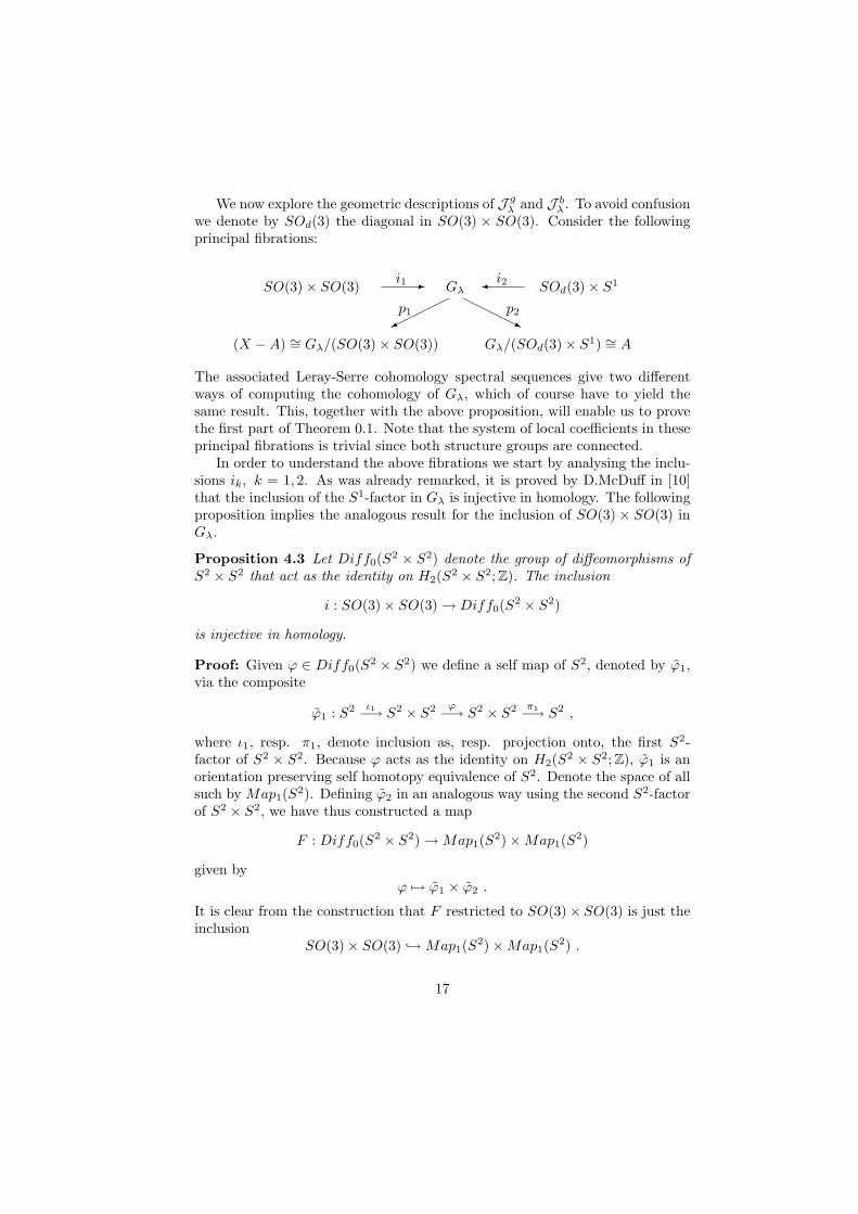
We now explore the geometric descriptions of J gλ and J b

λ . To avoid confusionwe denote by SOd(3) the diagonal in SO(3) × SO(3). Consider the followingprincipal fibrations:

SO(3)× SO(3) -i1 Gλ�i2 SOd(3)× S1

�����

p1H

HHHjp2

(X −A) ∼= Gλ/(SO(3)× SO(3)) Gλ/(SOd(3)× S1) ∼= A

The associated Leray-Serre cohomology spectral sequences give two differentways of computing the cohomology of Gλ, which of course have to yield thesame result. This, together with the above proposition, will enable us to provethe first part of Theorem 0.1. Note that the system of local coefficients in theseprincipal fibrations is trivial since both structure groups are connected.

In order to understand the above fibrations we start by analysing the inclu-sions ik, k = 1, 2. As was already remarked, it is proved by D.McDuff in [10]that the inclusion of the S1-factor in Gλ is injective in homology. The followingproposition implies the analogous result for the inclusion of SO(3) × SO(3) inGλ.

Proposition 4.3 Let Diff0(S2 × S2) denote the group of diffeomorphisms ofS2 × S2 that act as the identity on H2(S2 × S2; Z). The inclusion

i : SO(3)× SO(3)→ Diff0(S2 × S2)

is injective in homology.

Proof: Given ϕ ∈ Diff0(S2 × S2) we define a self map of S2, denoted by ϕ1,via the composite

ϕ1 : S2 ι1−→ S2 × S2 ϕ−→ S2 × S2 π1−→ S2 ,

where ι1, resp. π1, denote inclusion as, resp. projection onto, the first S2-factor of S2 × S2. Because ϕ acts as the identity on H2(S2 × S2; Z), ϕ1 is anorientation preserving self homotopy equivalence of S2. Denote the space of allsuch by Map1(S2). Defining ϕ2 in an analogous way using the second S2-factorof S2 × S2, we have thus constructed a map

F : Diff0(S2 × S2)→Map1(S2)×Map1(S2)

given byϕ 7→ ϕ1 × ϕ2 .

It is clear from the construction that F restricted to SO(3)× SO(3) is just theinclusion

SO(3)× SO(3) ↪→Map1(S2)×Map1(S2) .

17

Although Map1(S2) is not homotopy equivalent to SO(3), the above inclusionis injective in homology (see [6] for these two facts). This implies the result.

QED

Since we are working over the reals it follows from the above that the mapsin cohomology

i∗1 : H∗(Gλ)→ H∗(SO(3)× SO(3))

andi∗2 : H∗(Gλ)→ H∗(SOd(3)× S1) ,

induced by the inclusions i1 and i2, are surjective. Using the Leray-HirschTheorem (see [15]) this implies that the spectral sequences of both fibrationscollapse at the E2 term, giving the following two vector space isomorphisms forH∗(Gλ):

H∗(Gλ) ∼= H∗(X −A)⊗H∗(SO(3)× SO(3)) (7)

andH∗(Gλ) ∼= H∗(A)⊗H∗(SOd(3)× S1) . (8)

One can now easily check, using (6), (7), (8) and Proposition 4.1, that

H2(X −A) = 0 = H3(X −A)

andHp+4(X −A) ∼= Hp(X −A), p ≥ 0 .

Hence we conclude that

H∗(X −A) ∼={

R if ∗ = 4k, 4k + 1, k ≥ 00 otherwise,

as desired.

4.2 The ring structure

As V.Ginzburg pointed out to me, to compute the ring structure on the coho-mology of Gλ/(SO(3)× SO(3)) it is enough to show that

H∗(Gλ) ∼= H∗(Gλ/(SO(3)× SO(3)))⊗H∗(SO(3)× SO(3)) (9)

as graded algebras. The reason is that since Gλ is a group, in particular an H-space, we have that H∗(Gλ) is a Hopf algebra. The Leray Structure Theoremfor Hopf algebras over a field of characteristic 0 then says that H∗(Gλ) is thetensor product of exterior algebras with generators of odd degree and polynomialalgebras with generators of even degree (see [18] for relevant definitions and aproof of this structure theorem). The isomorphism (9) will then imply thatH∗(Gλ/(SO(3)×SO(3))) is the tensor product of an exterior algebra with one

18

generator of degree 1 and a polynomial algebra with one generator of degree 4,as stated in Theorem 0.1.

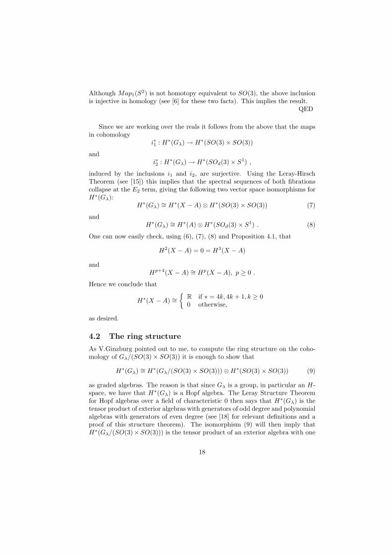
We know from the previous subsection that the Leray-Serre cohomologyspectral sequence for the fibration

SO(3)× SO(3) -i1 Gλ

?

p1

Gλ/(SO(3)× SO(3))

collapses with

E∗,∗∞∼= E∗,∗2

∼= H∗(Gλ/(SO(3)× SO(3)))⊗H∗(SO(3)× SO(3))

as bigraded algebras.Although proving (7), a vector space isomorphism, this does not directly

prove (9), a graded algebra isomorphism. What this says is that the bigradedalgebra E∗,∗0 (H∗(Gλ), F ), associated to H∗(Gλ) with filtration F coming fromthe above fibration, is isomorphic to H∗(Gλ/(SO(3)× SO(3)))⊗H∗(SO(3)×SO(3)) (see [15]).

The last step in the proof of (9) is now the following. H∗(Gλ) has a subal-gebra p∗(H∗(Gλ/(SO(3)×SO(3)))) ∼= H∗(Gλ/(SO(3)×SO(3))). From Propo-sition 4.3 we know that

i∗ : H∗(Gλ)→ H∗(SO(3)× SO(3))

is surjective. Choose α, β ∈ H3(Gλ) so that i∗(α) and i∗(β) generate the ringH∗(SO(3)×SO(3)). The subalgebra of H∗(Gλ) generated by α and β is isomor-phic to H∗(SO(3)×SO(3)) since the only relations in this algebra hold univer-sally on any cohomology algebra (skew-symmetry of the cup product of elementsof odd degree). Composing these inclusions of H∗(Gλ/(SO(3) × SO(3))) andH∗(SO(3)×SO(3)) as subalgebras of H∗(Gλ) with cup product multiplicationin H∗(Gλ) we get a map

ν : H∗(Gλ/(SO(3)× SO(3)))⊗H∗(SO(3)× SO(3))→ H∗(Gλ) .

Because H∗(Gλ) is (graded) commutative we have that ν is an algebra homo-morphism. Moreover, by construction, ν is compatible with filtrations (the obvi-ous one on H∗(Gλ/(SO(3)×SO(3)))⊗H∗(SO(3)×SO(3)) and F on H∗(Gλ)).As was already remarked, the degeneration of the spectral sequence at the E2

term implies that the associated bigraded version of ν is an algebra isomor-phism, which in turn shows that ν itself is an algebra isomorphism, concludingthe proof of (9) and hence of Theorem 0.1.

19

Appendix

The purpose of this Appendix is to justify the statement “J bλ is a codimension 2,

co-oriented submanifold of Jλ”, which was needed in the beginning of Section 4.We use the set-up and some results of [14], Chapter 3.

Fix an integer l ≥ 1. Let J lλ be the smooth Banach manifold of Cl-almost

complex structures on M = S2 × S2 that are compatible with ωλ. Its tangentspace TJJ l

λ at J consists of Cl-sections Y of the bundle End(TM, J, ωλ) whosefiber at p ∈M is the space of linear maps Y : TpM → TpM such that

Y J + JY = 0 , ωλ(Y v,w) + ωλ(v, Y w) = 0.

This space of Cl-sections is a Banach space and gives rise to a local modelfor the space J l

λ via the map Y 7→ J exp(−JY ). Let X l+1,p, p > 2, be theBanach manifold of W l+1,p-maps u : S2 → M , with [u(S2)] = [D]. This is thecompletion of the space of smooth maps with respect to the Sobolev W l+1,p-norm given by the sum of the Lp-norms of all derivatives of u up to order l+ 1.Its tangent space at u ∈ X l+1,p is W l+1,p(u∗TM), the space of W l+1,p sectionsof the bundle u∗TM over S2. Recall that, since p > 2, any u ∈ X l+1,p is of classCl by the Sobolev estimates.

Over X l+1,p × J lλ there is an infinite dimensional vector bundle E l,p whose

fiber at (u, J) is the space

E l,p(u,J) = W l,p(∧0,1T ∗S2 ⊗J u

∗TM)

of complex anti-linear 1-forms on S2, of class W l,p, with values in the pullbacktangent bundle u∗TM . This bundle has a natural section

F : X l+1,p × J lλ −→ E l,p

given by

F(u, J) = ∂J(u) =12(du ◦ j0 − J ◦ du) ,

where j0 is the standard complex structure on S2. Its zero-set is the universalmoduli space Ml([D],J l

λ). In [14], Chapter 3, it is proved that the differential

DF(u, J) : W l+1,p(u∗TM)×Cl(End(TM, J, ωλ))→W l,p(∧0,1T ∗S2⊗J u∗TM)

at a zero (u, J) is surjective, and so it follows from the implicit function theoremthat the spaceMl([D],J l

λ) is a smooth Banach manifold. This differential DFis given by the formula

DF(u, J)(ξ, Y ) = Duξ +12Y (u) ◦ du ◦ j0

for ξ ∈ W l+1,p(u∗TM) and Y ∈ Cl(End(TM, J, ωλ)), where Du is a 0th-orderperturbation (coming from the possible non-integrability of J) of the usual Dol-beault ∂-operator, and so is Fredholm.

20

Consider now the projection

π :Ml([D],J lλ) −→ J l

λ,

whose image is exactly the space J l,bλ of “bad” almost complex structures of

class Cl. The tangent space

T(u,J)Ml([D],J lλ)

consists of all pairs (ξ, Y ) such that

Duξ +12Y (u) ◦ du ◦ j0 = 0

and the derivative

dπ(u, J) : T(u,J)Ml([D],J lλ) −→ TJJ l

λ

is just the projection (ξ, Y ) 7→ Y . Hence the kernel of dπ(u, J) is isomorphic tothe kernel of Du whose dimension we will now determine.

Using the metric induced by J and ωλ on M , and the fact that u is a Cl-embedding (see Fact 1.5 in subsection 1.1), we have the isomorphisms of complexvector bundles

u∗TM ∼= TM |u(S2)∼= Tu ⊕Nu ,

where Tu = Im(du) and Nu = (Tu)⊥ are complex line sub-bundles of TM |u(S2)

because u is J-holomorphic and J is orthogonal with respect to the metric.Given ξ ∈ W l+1,p(u∗TM) we decompose it accordingly as ξ = ξt + ξn, whereξt ∈W l+1,p(Tu) and ξn ∈W l+1,p(Nu). An easy computation, using the explicitformula for Du given in Chapter 3 of [14], gives the decomposition

Duξ = Dnuξ

n +Ht(ξn) +Dtuξ

t , (10)

where Dtu : W l+1,p(Tu) → W l,p(∧0,1T ∗S2 ⊗J Tu) is a Dolbeault ∂-operator on

Tu, Dnu : W l+1,p(Nu)→W l,p(∧0,1T ∗S2⊗J Nu) is a 0th-order perturbation of a

Dolbeault ∂-operator on Nu and Ht : W l+1,p(Nu)→W l,p(∧0,1T ∗S2⊗J Tu) is a0th-order linear map related to the second fundamental form of u(S2) ⊂M . Thepoint to note is that if ξ = ξt ∈ W l+1,p(Tu) then Duξ

t ∈ W l+1,p(∧0,1T ∗S2 ⊗J

Tu), i.e. Duξt has no normal component. This implies that if ξ = ξn + ξt ∈

Ker(Du), then ξn ∈ Ker(Dnu). The main result proved in [7] implies that Dn

u

is injective, because the degree c1(Nu) = [D] · [D] = −2 is negative. When Jis integrable, and consequently Dn

u is equal to a ∂-operator, this is clear sincethere can be no nonzero holomorphic sections of a holomorphic line bundle withnegative degree. In [7] this result is extended to “generalized ∂-operators” oncomplex line bundles over Riemann surfaces, i.e. operators such as Dn

u .We have thus concluded that if ξ = ξn + ξt ∈ Ker(Du) then ξn = 0, and

from (10) this means that Ker(Du) ∼= Ker(Dtu). The kernel of Dt

u is naturally

21

identified with the vector space of holomorphic vector fields on S2, which is thetangent space of the reparametrization group G = PSL(2,C) of real dimension6.

The image of dπ(u, J) consists of all Y such that Y (u) ◦ du ◦ j0 ∈ Im(Du).This is a closed subspace of TJJ l

λ and, since DF(u, J) is onto, it has the same(finite) codimension as the image of Du. Indeed we have a natural isomorphism

Cl(End(TM, J, ωλ))/Im(dπ(u, J)) −→W l,p(∧0,1T ∗S2 ⊗J u∗TM)/Im(Du)

given by

Y 7−→ 12Y (u) ◦ du ◦ j0 .

It follows that dπ(u, J) is a Fredholm operator and has the same index as Du,which in this case is 4. This means that the map between smooth Banachmanifolds

J l,bλ =Ml([D],J l

λ)/G −→ J lλ

induced by π is a codimension 2 inclusion. Then an application of the inversemapping theorem (see [9], Chapter 2) shows that J l,b

λ is a codimension 2 sub-manifold of J l

λ.To prove that J l,b

λ is co-oriented in J lλ it is enough to show, because of the

above identification, that Coker(Du) is oriented. For that we again follow [14],Chapter 3. The determinant line of a complex linear Fredholm operator carriesa natural orientation. Due to the possible non-integrability of J , Du is not ingeneral a complex linear operator, but it does lie in a component of the spaceof Fredholm operators which contains the complex linear operator ∂. Thereforeits determinant line

det(Du) = ∧max(Ker(Du))⊗ ∧max(Coker(Du)) (11)

carries a natural orientation. Since Ker(Du) has a natural orientation as thetangent space of G = PSL(2,C), we have that (11) determines an orientationfor Coker(Du).

This justifies the use of Alexander-Pontrjagin duality in the beginning ofSection 4, provided we work with the spaces J l,g

λ and J l,bλ . As was already

remarked in the Introduction, the algebraic topological invariants of these spacesare the same as the ones of J g

λ and J bλ and so Proposition 4.1 is correct as stated.

22

References

[1] M.Audin, The topology of torus actions on symplectic manifolds, Progressin Math. 93, Birkhauser, 1991.

[2] M.Audin and F.Lafontaine (eds), Holomorphic Curves in Symplectic Ge-ometry, Progress in Math. 117, Birkhauser, 1994.

[3] J.Eells, Alexander-Pontrjagin duality in function spaces, Proc. Symposia inPure Math. 3, Amer. Math. Soc. (1961), 109-129.

[4] R.Gompf, A New Construction of Symplectic Manifolds, Annals of Math.,142 (1995), 527-595.

[5] M.Gromov, Pseudo holomorphic curves in symplectic manifolds, Inv.Math., 82 (1985), 307-347.

[6] V.Hansen, The space of self maps on the 2-sphere, Groups of self-equivalences and related topics (Montreal,PQ,1988), 40-47, Lecture Notesin Math. 1425, Springer, 1990.

[7] H.Hofer, V.Lizan and J.-C.Sikorav, On genericity for holomorphic curves in4-dimensional almost-complex manifolds, Lab. de Topologie et Geometrie,preprint 37, Univ. Paul Sabatier, Toulouse (France), 1994.

[8] P.Iglesias, Les SO(3)-varietes symplectiques et leur classification en dimen-sion 4, Bull. Soc. Math. France, 119 (1991), 371-396.

[9] S.Lang, Differential and Riemannian Manifolds, Graduate Texts in Math.160, Springer-Verlag, 1995.

[10] D.McDuff, Examples of symplectic structures, Inv. Math 89 (1987), 13-36.

[11] D.McDuff, The local behaviour of holomorphic curves in almost complex4-manifolds, Journal of Differential Geometry 34 (1991), 311-358.

[12] D.McDuff, J-holomorphic spheres in symplectic 4-manifolds: a survey, toappear in the proceedings of the 1994 Symplectic Topology Program at theNewton Institute, ed. C.Thomas, Cambridge University Press.

[13] D.McDuff and D.A.Salamon, Introduction to Symplectic Topology, OxfordUniversity Press, 1995.

[14] D.McDuff and D.A.Salamon, J-holomorphic curves and quantum cohomol-ogy, University Lecture Series 6, American Mathematical Society, Provi-dence, RI, 1994.

[15] J.McCleary, User’s Guide to Spectral Sequences, Mathematics Lecture Se-ries 12, Publish or Perish, 1985.

23

[16] J.Moser, On the volume elements on a manifold, Trans. Amer. Math. Soc.,120 (1965), 286-294.

[17] S.Smale, Diffeomorphisms of the 2-sphere, Proc. Amer. Math. Soc., 10(1959), 621-626.

[18] E.Spanier, Algebraic Topology, McGraw-Hill, 1966.

24