TOPOLOGY OF ROBOT MOTION PLANNING Michael …shmuel/AAT-readings/Robotics...TOPOLOGY OF ROBOT MOTION PLANNING Michael Farber University of Durham Abstract. In this paper we discuss

TOPOLOGY OF ROBOT MOTION PLANNING

Michael FarberUniversity of Durham

Abstract. In this paper we discuss topological problems inspired by robotics. We study in detailthe robot motion planning problem. With any path-connected topological spaceX we associatea numerical invariantTC(X) measuring the “complexity of the problem of navigation inX.” Weexamine how the numberTC(X) determines the structure of motion planning algorithms, bothdeterministic and random. We compute the invariantTC(X) in many interesting examples. In thecase of the real projective spaceRPn (wheren , 1, 3, 7) the numberTC(RPn) − 1 equals theminimal dimension of the Euclidean space into whichRPn can be immersed.

Key words: Robot motion planning algorithms, navigational complexity of configuration spaces,collision avoiding, cohomological lower bound, immersions of projective spaces

2000 Mathematics Subject Classification:Primary 68T40, 93C85; Secondary 55Mxx

1. Introduction

This paper represents a slightly extended version of a mini-course consisting offour lectures delivered at the Universite de Montreal in June 2004. The maingoal was to give an introduction to the topological robotics and in particularto describe a topological approach to the robot motion planning problem. Thisnew theory appears to be useful both in robotics and in topology. In robotics, itexplains how the instabilities in the robot motion planning algorithms depend onthe homotopy properties of the robot’s configuration space. In topology, if oneregards the topological spaces as configuration spaces of mechanical systems,one discovers a new interesting homotopy invariantTC(X) which measures the“navigational complexity” of X. The invariantTC(X) is similar in spirit to theLusternik – Schnirelmann category cat(X) although in factTC(X) and cat(X) areindependent, as simple examples (given below) show.

The topological approach to the robot motion planning problem was initiatedby the author in Farber (2003; 2004). It was inspired by the earlier well-knownwork of Smale (1987) and Vassil′iev (1988) on the theory of topological complex-ity of algorithms of solving polynomial equations. The approach of Farber (2003;2004) was also based on the general theory of robot motion planning algorithmsdescribed in the book of J.-C. Latombe (1991). It is my pleasure to acknowledge

c© 2005Springer. Printed in the Netherlands.

196 M. FARBER

the importance of discussions of the initial versions of Farber (2003; 2004) withDan Halperin and Micha Sharir in summer 2001 in Tel Aviv. The theory of a genusof a fiber space developed by Schwarz (1966) plays a technically important rolein our approach as well as in the work of Smale and Vassiliev.

Further developments and applications of the theory of topological complexityof robot motion planning of Farber (2003; 2004) are also mentioned in these notes.They include the study of collision free motion planning algorithms in Euclideanspaces (Farber and Yuzvinsky, 2004) and on graphs (Farber, 2005) and also ap-plications to the immersion problem for the real projective spaces (Farber et al.,2003).

These notes also include some new material. We explain how one may con-struct an explicit motion planning algorithm in the configuration space ofn dis-tinct particles inRm having topological complexity≤ n2. Such an algorithmmay have some practical applications. We also analyze the complexity of con-trolling many objects simultaneously. Finally we mention some interesting openproblems.

The plan of the lectures in Montreal was as follows:

Lecture 1 Introduction. Interesting topological spaces provided by robotics andquestions about the standard topological spaces one asks after encounterswith robotics.

Lecture 2 The notion of topological complexity of the motion planning problem.The Schwarz genus. Computations of the topological complexity in basicexamples.

Lecture 3 Topological complexity of collision free motion planning of many par-ticles in Euclidean spaces and on graphs.

Lecture 4 Motion planning in projective spaces. Relation with the immersionproblem for the real projective spaces. Discussion of open problems.

2. First examples of configuration spaces

The ultimate goal of robotics is creating of autonomous robots (Latombe, 1991).Such robots should be able to accept high-level descriptions of tasks and executethem without further human intervention. The input description specifieswhatshould be done and the robot decideshow to do it and performs the task. Oneexpects robots to have sensors and actuators.

A few words about history of robotics. The idea of robots goes back to ancienttimes. The wordrobotwas first used in 1921 by Karel Capek in his play “Possum’sUniversal Robots.” The wordroboticswas coined by Isaac Asimov in 1940 in hisbook “I, robot.”

TOPOLOGY OF ROBOT MOTION PLANNING 197

What is common to robotics and topology? Topology enters robotics throughthe notion ofconfiguration space. Any mechanical systemR determines the vari-ety of all its possible statesX which is called the configuration space ofR. Usuallya state of the system is fully determined by finitely many real parameters; in thiscase the configuration spaceX can be viewed as a subset of the Euclidean spaceRk. Each point ofX represents a state of the system and different points repre-sent different states. The configuration spacesX comes with the natural topology(inherited fromRk) which reflects the technical limitations of the system.

Many problems of control theory can be solved knowing only the configura-tion space of the system. Peculiarities in the behavior of the system can often beexplained by topological properties of the system’s configuration space. We willdiscuss this in more detail in the case of the motion planning problem. We willsee howone may predict the character of instabilities of the behavior of the robotknowing the cohomology algebra of its configuration space.

If the configuration space of the system is known one may often forget aboutthe system and study instead the configuration space viewed with its topology andwith some other geometric structures, e.g., with the Riemannian metric.

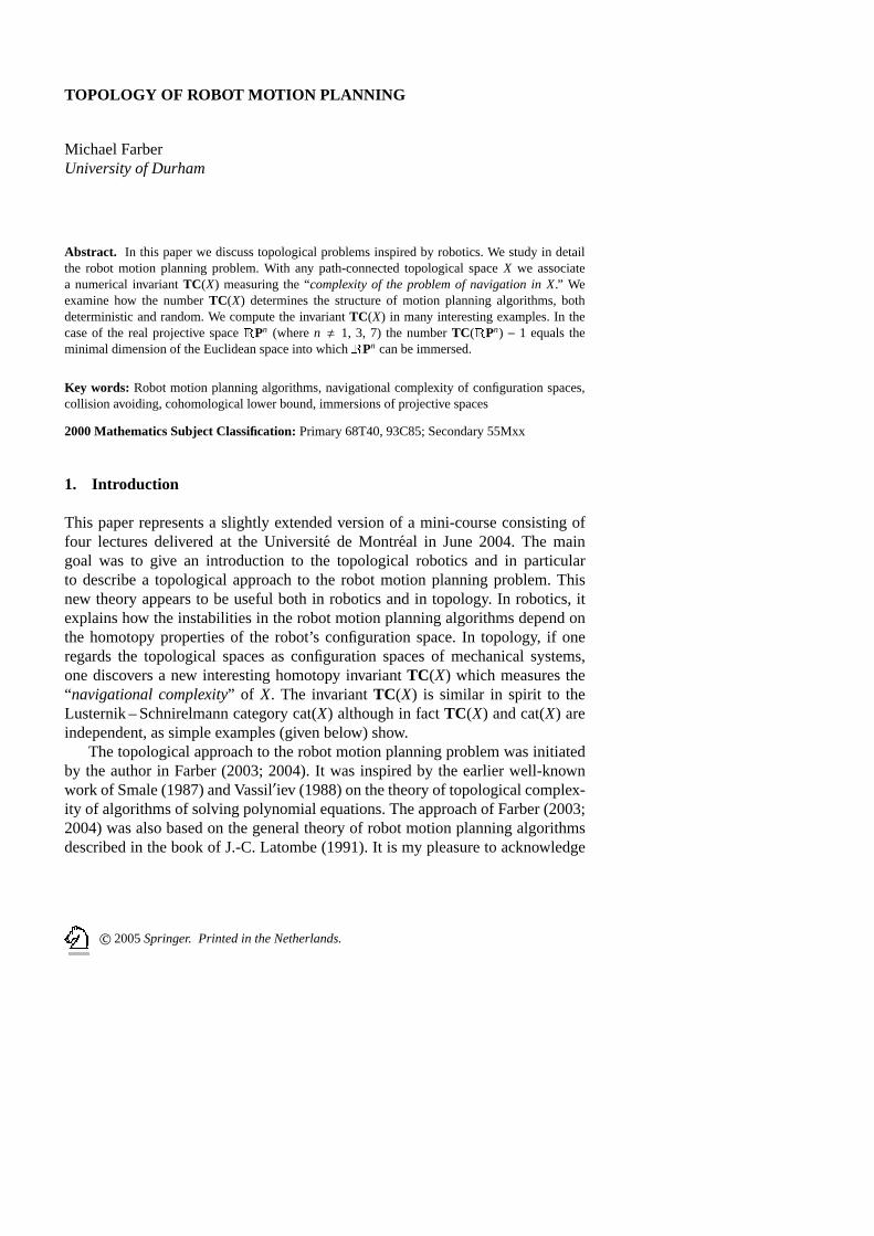
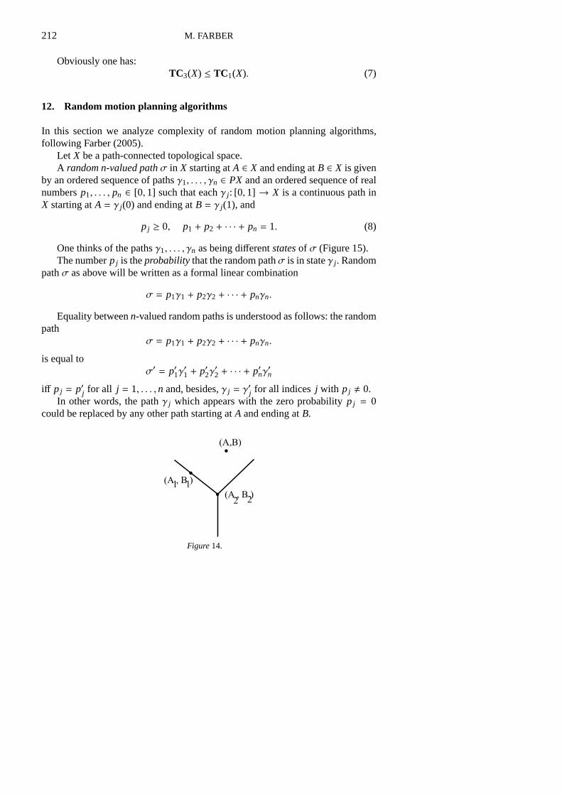
EXAMPLE 2.1 (Piano movers’ problem; Schwartz and Sharir, 1983). In Figure1 the large rectangles represent the obstacles and the black figures represent dif-ferent states of the “piano.”

We assume that the picture is planar, i.e., the objects move in the horizontalplane only. Of course in practice the obstacles may have much more involvedgeometry than it is shown on the picture. One has to move the piano from onestate to another avoiding the obstacles. The configuration space in this example is3-dimensional having complicated geometry. The state of the piano is determinedby the coordinates of the center and by the orientation.

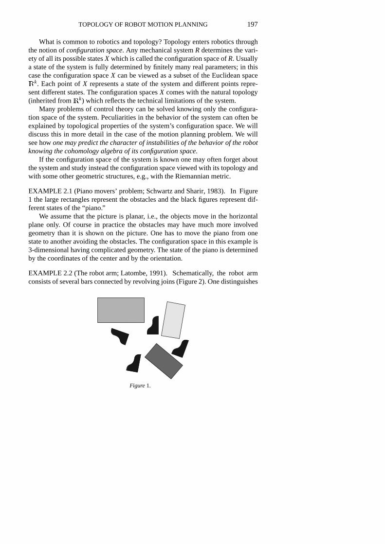
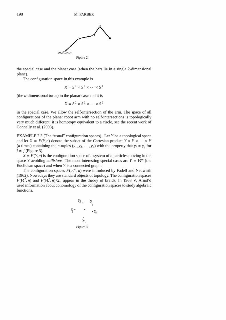
EXAMPLE 2.2 (The robot arm; Latombe, 1991). Schematically, the robot armconsists of several bars connected by revolving joins (Figure 2). One distinguishes

Figure1.

198 M. FARBER

Figure2.

the spacial case and the planar case (when the bars lie in a single 2-dimensionalplane).

The configuration space in this example is

X = S1 × S1 × · · · × S1

(then-dimensional torus) in the planar case and it is

X = S2 × S2 × · · · × S2

in the spacial case. We allow the self-intersection of the arm. The space of allconfigurations of the planar robot arm with no self-intersections is topologicallyvery much different: it is homotopy equivalent to a circle, see the recent work ofConnelly et al. (2003).

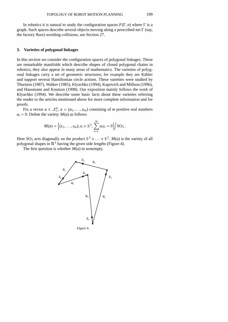
EXAMPLE 2.3 (The “usual” configuration spaces). LetY be a topological spaceand letX = F(Y,n) denote the subset of the Cartesian productY × Y × · · · × Y(n times) containing then-tuples (y1, y2, . . . , yn) with the property thatyi , y j fori , j (Figure 3).

X = F(Y,n) is the configuration space of a system ofn particles moving in thespaceY avoidingcollisions. The most interesting special cases areY = Rm (theEuclidean space) and whenY is a connected graph.

The configuration spacesF(Rm,n) were introduced by Fadell and Neuwirth(1962). Nowadays they are standard objects of topology. The configuration spacesF(R2, n) and F(R2, n)/Σn appear in the theory of braids. In 1968 V. Arnol′dused information about cohomology of the configuration spaces to study algebraicfunctions.

Figure3.


In robotics it is natural to study the configuration spacesF(Γ,n) whereΓ is agraph. Such spaces describe several objects moving along a prescribed netΓ (say,the factory floor) avoiding collisions, see Section 27.

3. Varieties of polygonal linkages

In this section we consider the configuration spaces of polygonal linkages. Theseare remarkable manifolds which describe shapes of closed polygonal chains inrobotics; they also appear in many areas of mathematics. The varieties of polyg-onal linkages carry a set of geometric structures; for example they are Kahlerand support several Hamiltonian circle actions. These varieties were studied byThurston (1987), Walker (1985), Klyachko (1994), Kapovich and Millson (1996),and Hausmann and Knutson (1998). Our exposition mainly follows the work ofKlyachko (1994). We describe some basic facts about these varieties referringthe reader to the articles mentioned above for more complete information and forproofs.

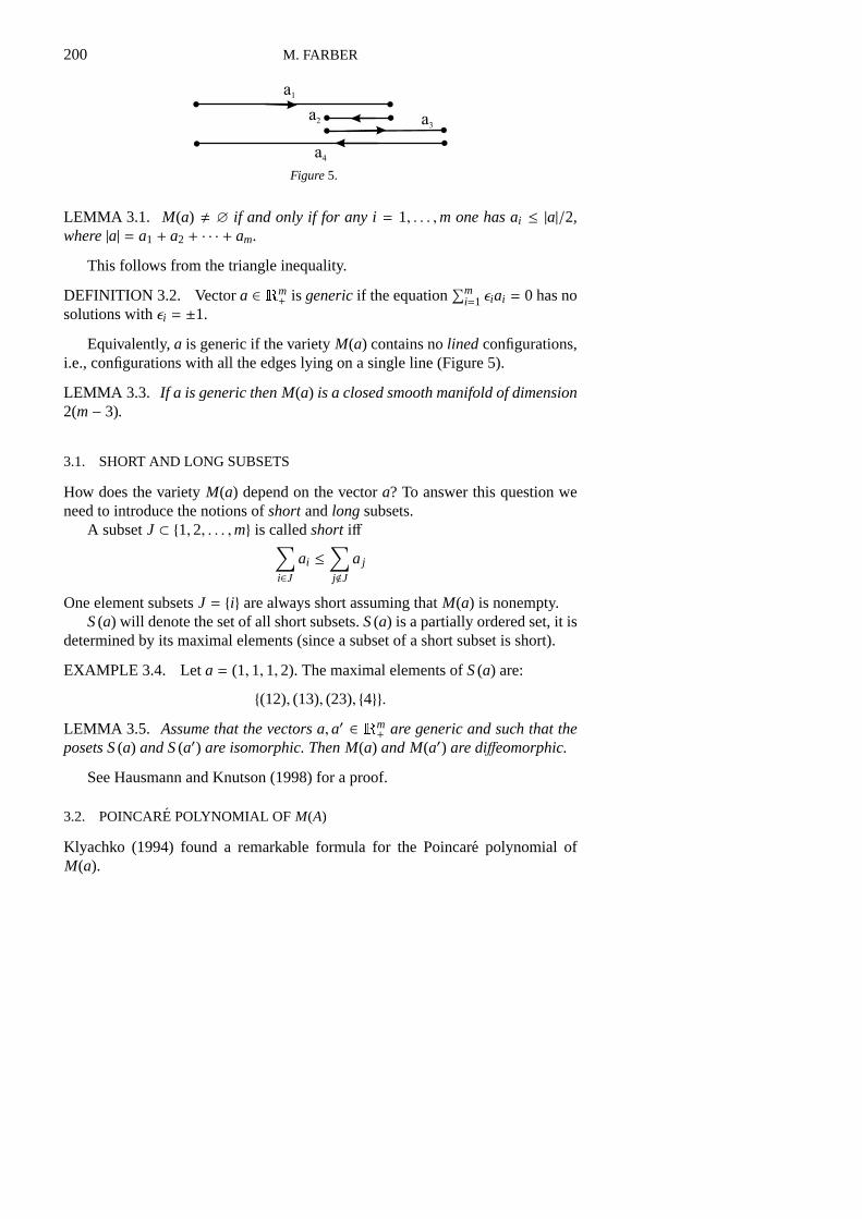
Fix a vectora ∈ Rm+ , a = (a1, . . . ,am) consisting ofm positive real numbers

ai > 0. Define the varietyM(a) as follows

M(a) =

{(z1, . . . , zm); zi ∈ S2,

m∑

i=1

aizi = 0}/

SO3 .

Here SO3 acts diagonally on the productS2 × . . . × S2. M(a) is the variety of allpolygonal shapes inR3 having the given side lengths (Figure 4).

The first question is whetherM(a) in nonempty.

Figure4.

200 M. FARBER

Figure5.

LEMMA 3.1. M(a) , ∅ if and only if for anyi = 1, . . . ,m one hasai ≤ |a|/2,where|a| = a1 + a2 + · · · + am.

This follows from the triangle inequality.

DEFINITION 3.2. Vectora ∈ Rm+ is genericif the equation

∑mi=1 εiai = 0 has no

solutions withεi = ±1.

Equivalently,a is generic if the varietyM(a) contains nolined configurations,i.e., configurations with all the edges lying on a single line (Figure 5).

LEMMA 3.3. If a is generic thenM(a) is a closed smooth manifold of dimension2(m− 3).

3.1. SHORT AND LONG SUBSETS

How does the varietyM(a) depend on the vectora? To answer this question weneed to introduce the notions ofshortandlongsubsets.

A subsetJ ⊂ {1,2, . . . ,m} is calledshort iff∑

i∈Jai ≤

∑

j<J

a j

One element subsetsJ = {i} are always short assuming thatM(a) is nonempty.S(a) will denote the set of all short subsets.S(a) is a partially ordered set, it is

determined by its maximal elements (since a subset of a short subset is short).

EXAMPLE 3.4. Leta = (1,1,1, 2). The maximal elements ofS(a) are:

{(12), (13), (23), {4}}.LEMMA 3.5. Assume that the vectorsa,a′ ∈ Rm

+ are generic and such that theposetsS(a) andS(a′) are isomorphic. ThenM(a) andM(a′) are diffeomorphic.

See Hausmann and Knutson (1998) for a proof.

3.2. POINCARE POLYNOMIAL OF M(A)

Klyachko (1994) found a remarkable formula for the Poincare polynomial ofM(a).


THEOREM 3.6. The Poincare polynomial ofM(a) equals

P(t) =1

t2(t2 − 1)

((1 + t2)m−1 −

∑

J∈S(a)

t2|J|)

(1)

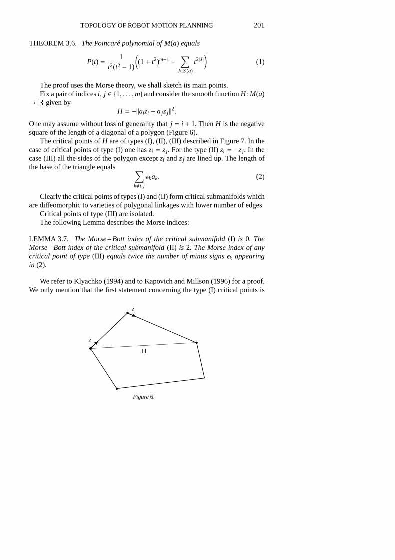
The proof uses the Morse theory, we shall sketch its main points.Fix a pair of indicesi, j ∈ {1, . . . ,m} and consider the smooth functionH: M(a)

→ R given byH = −‖aizi + a jzj‖2.

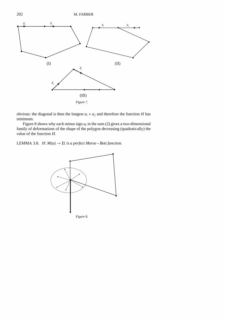
One may assume without loss of generality thatj = i + 1. ThenH is the negativesquare of the length of a diagonal of a polygon (Figure 6).

The critical points ofH are of types (I), (II), (III) described in Figure 7. In thecase of critical points of type (I) one haszi = zj . For the type (II)zi = −zj . In thecase (III) all the sides of the polygon exceptzi andzj are lined up. The length ofthe base of the triangle equals ∑

k,i, j

εkak. (2)

Clearly the critical points of types (I) and (II) form critical submanifolds whichare diffeomorphic to varieties of polygonal linkages with lower number of edges.

Critical points of type (III) are isolated.The following Lemma describes the Morse indices:

LEMMA 3.7. The Morse – Bott index of the critical submanifold(I) is 0. TheMorse – Bott index of the critical submanifold(II) is 2. The Morse index of anycritical point of type(III) equals twice the number of minus signsεk appearingin (2).

We refer to Klyachko (1994) and to Kapovich and Millson (1996) for a proof.We only mention that the first statement concerning the type (I) critical points is

Figure6.

202 M. FARBER

(I) (II)

(III)

Figure7.

obvious: the diagonal is then the longestai + a j and therefore the functionH hasminimum.

Figure 8 shows why each minus signεk in the sum (2) gives a two-dimensionalfamily of deformations of the shape of the polygon decreasing (quadratically) thevalue of the functionH.

LEMMA 3.8. H: M(a)→ R is a perfect Morse – Bott function.

Figure8.


Figure9.

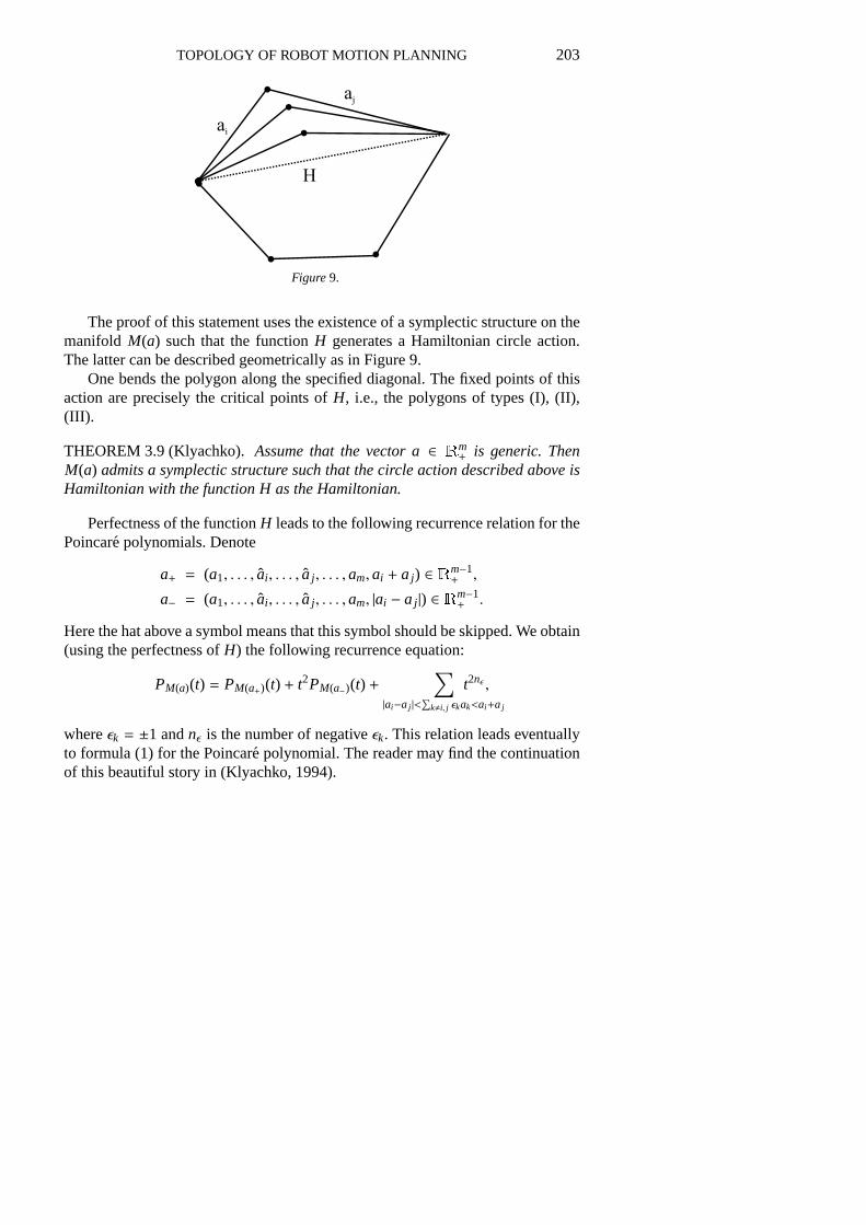
The proof of this statement uses the existence of a symplectic structure on themanifold M(a) such that the functionH generates a Hamiltonian circle action.The latter can be described geometrically as in Figure 9.

One bends the polygon along the specified diagonal. The fixed points of thisaction are precisely the critical points ofH, i.e., the polygons of types (I), (II),(III).

THEOREM 3.9 (Klyachko).Assume that the vectora ∈ Rm+ is generic. Then

M(a) admits a symplectic structure such that the circle action described above isHamiltonian with the functionH as the Hamiltonian.

Perfectness of the functionH leads to the following recurrence relation for thePoincare polynomials. Denote

a+ = (a1, . . . , ai , . . . , a j , . . . ,am,ai + a j) ∈ Rm−1+ ,

a− = (a1, . . . , ai , . . . , a j , . . . ,am, |ai − a j |) ∈ Rm−1+ .

Here the hat above a symbol means that this symbol should be skipped. We obtain(using the perfectness ofH) the following recurrence equation:

PM(a)(t) = PM(a+)(t) + t2PM(a−)(t) +∑

|ai−a j |<∑k,i, j εkak<ai+a j

t2nε ,

whereεk = ±1 andnε is the number of negativeεk. This relation leads eventuallyto formula (1) for the Poincare polynomial. The reader may find the continuationof this beautiful story in (Klyachko, 1994).

204 M. FARBER

4. Universality theorems for configuration spaces

How special are configuration spaces of the mechanisms? In other words, we askif there exist specific topological properties which characterize the configurationspaces among the topological spaces?

Universality theorems for configuration spaces claim (roughly) that all “rea-sonable” topological spaces are configuration spaces of linkages. Many theoremsof this type are known. Lebesgue (1950) gave an account of several results includ-ing Kempe’s universality theorem, not for the configuration space of the mecha-nism itself but for the orbit of one of its vertices: “Toute courbe algebrique peutetre tracee a l’aide d’un systeme articule.”

A theorem of Jordan and Steiner (1999) states:

THEOREM 4.1. Any compact real algebraic varietyV ⊂ Rn is homeomorphicto a union of components of the configuration space of a mechanical linkage.

Kapovich and Millson (2002) prove the following statement:

THEOREM 4.2. For any smooth compact manifoldM there exists a linkagewhose moduli space is diffeomorphic to a disjoint union of a number of copiesof M.

Let us explain the terms used here. Anabstract linkageis a triple

L = (L, `,W)

whereL is a graph,W ⊂ V(L) is an ordered subset of vertices ofL, and`: E(L)→R+ is a function on the set of edges ofL. HereW are thefixedvertices ofL and`is a “metric” (length function) onL. A planar realizationof L is a map

φ: V(L)→ R2

such that if the verticesv,w ∈ V(L) are joined by an edgee ∈ E(L) in L then

|φ(v) − φ(w)| = `(e).

Let W = (v1, . . . , vn) and letZ = (z1, . . . , zn) be an ordered set ofn pointszi ∈ R2.A planar realizationof L relative toZ is a realizationφ: V(L) → R2 as abovesatisfying an additional requirement thatφ(v j) = zj for all j = 1, . . . ,n. The setC(L,Z) of all relative planar realizations ofL is called therelative configurationspaceof L. Elements ofC(L,Z) are all planar realizations ofL such that thevertices ofW stay in the prescribed positionsZ.

The linkages which we studied in Section 3 are special cases when the graphL is homeomorphic to the circle.


Kapovich and Millson (2002) observe that the configuration space of any pla-nar linkage admits an involution (induced by a reflection of the plane) and thisinvolution is nontrivial if the graphL is connected and the configuration spaceis not a point. Hence ifMn is a closed manifoldn > 0 which does not admit anontrivial involution (such manifolds exist) thenM is not homeomorphic to themoduli space of a planar linkage.

5. A remark about configuration spaces in robotics

The notion of configuration space may seem obvious and even trivial for a topol-ogist. But for people in robotics it is not so. In fact in some problems of roboticsthis notion appears to be even controversial. For a system of great complexity it isunrealistic to assume that its configuration space can be described completely;more reasonably to think that at any particular moment the topology and thegeometry of the configuration space are known only partially or approximately.

We want to emphasize that we do not question the existence of the configura-tion spaces. However in some particular cases it may happen to be too expensiveto learn the topology of the configuration space entirely. Then one has to solve thecontrol problems “on-line” and to learn the underlying configuration space at thesame time.

It seems plausible that there may exist a better mathematical notion of a con-figuration space describing a “partially known” topological space whose geometryis being gradually revealed.

6. The motion planning problem

In this section we start studying the robot motion planning problem which is themain topic of these lectures.

Imagine that you get into your advanced car and say “Go home!” and the cartakes you home, automatically, obeying the traffic rules. Such a car must have aGPS (finding its current location) and a computer program suggesting a specificroute from any initial state to any desired state. Computer programs of this kindare based onmotion planning algorithms. In general, given a mechanical system,a motion planning algorithm is a function which assigns to any pair of states ofthe system (i.e., the initial state and the desired state) a continuous motion of thesystem starting at the initial state and ending at the desired state. A recent surveyof algorithmic motion planning can be found in Sharir (1997); see also Latombe(1991).

Farber (2003; 2004) reveal the topological nature of the robot motion planningproblem. They show that the navigational complexity of configuration spaces,TC(X), is a homotopy invariant quantity which can be studied using the algebraic

206 M. FARBER

Figure10.

topology tools. This theory explains how knowing the cohomology algebra ofconfiguration space of a robot one may predict instabilities of its behavior.

Below in this article we describe the results of Farber (2003; 2004) addingsome more recent developments.

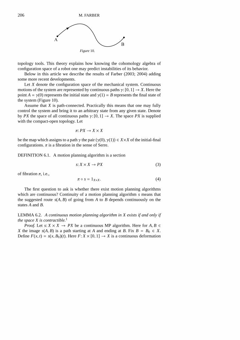
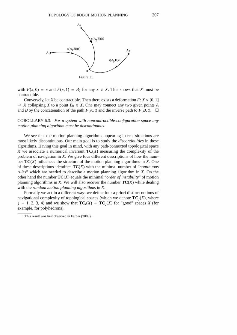
Let X denote the configuration space of the mechanical system. Continuousmotions of the system are represented by continuous pathsγ: [0, 1]→ X. Here thepoint A = γ(0) represents the initial state andγ(1) = B represents the final state ofthe system (Figure 10).

Assume thatX is path-connected. Practically this means that one may fullycontrol the system and bring it to an arbitrary state from any given state. Denoteby PX the space of all continuous pathsγ: [0,1] → X. The spacePX is suppliedwith the compact-open topology. Let

π: PX→ X × X

be the map which assigns to a pathγ the pair(γ(0), γ(1)

) ∈ X×X of the initial-finalconfigurations.π is a fibration in the sense of Serre.

DEFINITION 6.1. A motion planning algorithm is a section

s: X × X→ PX (3)

of fibrationπ, i.e.,π ◦ s = 1X×X. (4)

The first question to ask is whether there exist motion planning algorithmswhich are continuous? Continuity of a motion planning algorithms means thatthe suggested routes(A, B) of going from A to B depends continuously on thestatesA andB.

LEMMA 6.2. A continuous motion planning algorithm inX exists if and only ifthe spaceX is contractible.1

Proof. Let s: X × X → PX be a continuous MP algorithm. Here forA, B ∈X the images(A, B) is a path starting atA and ending atB. Fix B = B0 ∈ X.DefineF(x, t) = s(x, B0)(t). HereF: X × [0,1] → X is a continuous deformation


Figure11.

with F(x,0) = x and F(x, 1) = B0 for any x ∈ X. This shows thatX must becontractible.

Conversely, letX be contractible. Then there exists a deformationF: X × [0,1]→ X collapsingX to a pointB0 ∈ X. One may connect any two given pointsAandB by the concatenation of the pathF(A, t) and the inverse path toF(B, t). ¤

COROLLARY 6.3. For a system with noncontractible configuration space anymotion planning algorithm must be discontinuous.

We see that the motion planning algorithms appearing in real situations aremost likely discontinuous. Our main goal is to study thediscontinuitiesin thesealgorithms. Having this goal in mind, with any path-connected topological spaceX we associate a numerical invariantTC(X) measuring the complexity of theproblem of navigation inX. We give four different descriptions of how the num-berTC(X) influences the structure of the motion planning algorithms inX. Oneof these descriptions identifiesTC(X) with the minimal number of “continuousrules” which are needed to describe a motion planning algorithm inX. On theother hand the numberTC(X) equals the minimal “order of instability” of motionplanning algorithms inX. We will also recover the numberTC(X) while dealingwith therandom motion planning algorithmsin X.

Formally we act in a different way: we define four a priori distinct notions ofnavigational complexity of topological spaces (which we denoteTC j(X), wherej = 1, 2, 3, 4) and we show thatTC i(X) = TC j(X) for “good” spacesX (forexample, for polyhedrons).

1 This result was first observed in Farber (2003).

208 M. FARBER

7. Tame motion planning algorithms

DEFINITION 7.1. A motion planning algorithms: X × X → PX is called tameif X × X can be split into finitely many sets

X × X = F1 ∪ F2 ∪ F3 ∪ · · · ∪ Fk (5)

such that

1. s|Fi : Fi → PX is continuous,i = 1, . . . , k,

2. Fi ∩ F j = ∅, wherei , j,

3. EachFi is an Euclidean Neighborhood Retract (ENR).2

For a fixed pair of points (A, B) ∈ Fi , the curve produced by the algorithmt 7→ s(A, B)(t) ∈ X is a continuous curve inX which starts at pointA ∈ X and endsat pointB ∈ X. This curve depends continuously on (A, B) assuming that the pairof points (A, B) varies in the setFi .

Recall the definition of ENR:

DEFINITION 7.2. A topological spaceX is called an ENR if it can be embeddedinto an Euclidean spaceX ⊂ Rk such that for some open neighborhoodX ⊂ U ⊂Rk there exists a retractionr: U → X, r |X = 1X.

All motion planning algorithms which appear in practice are tame. The con-figuration spaceX is usually a semi-algebraic set and the setsF j ⊂ X × X aregiven by equations and inequalities involving real algebraic functions; thus theyare semi-algebraic as well. In practical situations the functionss|F j : F j → PX arereal algebraic and hence they are continuous.

DEFINITION 7.3. The topological complexity of a tame motion planning algo-rithm (3) is the minimal number of domains of continuityk in a representation oftype (5).

DEFINITION 7.4. The topological complexityTC1(X) of a path-connectedtopological spaceX is the minimal topological complexity of motion planningalgorithms inX.

Observation.TC1(X) = 1 if and only if X is an ENR and it is contractible.

We setTC1(X) = ∞ if X admits no tame motion planning algorithms.

EXAMPLE 7.5. Let us show thatTC1(Sn) = 2 for n odd andTC1(Sn) ≤ 3 forn even.


Figure12.

Figure13.

Let F1 ⊂ Sn × Sn be the set of all pairs (A, B) such thatA , −B. We mayconstruct a continuous sections1: F1 → PSn by movingA toward B along theshortest geodesic arc.

Consider now the setF2 ⊂ Sn × Sn consisting of all pairs antipodal (A,−A).If n is odd we may construct a continuous sections2: F2→ PSn as follows. Fix anonvanishing tangent vector fieldv onSn. MoveA toward the antipodal point−Aalong the semi-circle tangent to vectorv(A).

In the case whenn is even find a tangent vector fieldv with a single zeroA0 ∈ Sn. DefineF2 = {(A,−A); A , A0} and defines2: F2 → PSn as above. ThesetF3 = {(A0,−A0)} consists of a single pair; defines3: F3 → PSn by choosingan arbitrary path fromA0 to −A0.

8. The Schwarz genus

Let p: E→ B be a fibration. Its Schwartz genus is defined as the minimal numberk such that there exists an open cover of the baseB = U1∪U2∪ · · · ∪Uk with theproperty that over each setU j ⊂ B there exists a continuous sectionsj : U j → Eof E → B. This notion was introduced by A. S. Schwarz in 1958. In 1987 –1988 S. Smale and V. A. Vassiliev applied the notion of Schwarz genus to studycomplexity of algorithms of solving polynomial equations.

2 An equivalent concept was introduced in Farber (2004) under the name “motion planner.”

210 M. FARBER

The genus of a fibration equals 1 if and only if it admits a continuous section.The genus of the Serre fibrationP0X → X coincides with the Lusternik –

Schnirelmann category cat(X) of X, see Cornea et al. (2003). HereP0(X) is thespace of paths inX which start at the base pointx0 ∈ X. For the motion planningproblem we need to study a different fibrationπ: PX→ X × X.

9. The second notion of topological complexity

The invariantTC1(X) introduced above seems to be quite natural from the roboticspoint of view. However a more convenient topological invariant uses open coversinstead of decompositions into ENR’s.

DEFINITION 9.1. Let X be a path-connected topological space. The numberTC2(X) is defined as the Schwartz genus of the fibration

π: PX→ X × X.

This notion coincides with the original definition of the topological complex-ity of the robot motion planning problem given in Farber (2003).

Explicitly, TC2(X) is the minimal numberk such that there exists an opencover

X × X = U1 ∪ U2 ∪ · · · ∪ Uk

with the property thatπ admits a continuous sectionsj : U j → PX over eachU j ⊂X × X.

Note that the inclusionU j → X × X may be not null-homotopic. For exam-ple, if X is a polyhedron, there always exists a continuous section over a smallneighborhood of the diagonalX ⊂ X × X.

We know thatTC2(X) = 1 if and only if X is contractible.

LEMMA 9.2. One has

cat(X) ≤ TC2(X) ≤ cat(X × X).Proof. We shall use two following simple properties of the Schwartz genus.

Consider a fibrationE→ B.

1. Let B′ ⊂ B be a subset,E′ = p−1(B′). Then the genus ofE′ → B′ is less thanor equal to the genus ofE→ B.

2. The genus ofE→ B is less than or equal to cat(B).

To probe the lemma, apply 1 to the fibrationPX → X × X and to the subsetX × x0 ⊂ X × X. Note thatπ−1(X × x0) = P0X. We findTC2(X) ≥ cat(X).

2 givesTC2(X) ≤ cat(X × X). ¤

Exercise.Let G be a connected Lie group. Then

TC2(G) = cat(G).


EXAMPLE 9.3. TC2(SO(3)

)= cat

(SO(3)

)= cat(RP3) = 4.

This example is important for robotics since SO(3) is the configuration spaceof a rigid body inR3 fixed at a point.

10. Homotopy invariance

THEOREM 10.1. The numberTC2(X) is a homotopy invariant ofX.

See Farber (2003) for a proof.

11. Order of instability of a motion planning algorithm

Let s: X × X→ PX be a tame motion planning algorithm and let

X × X = F1 ∪ F2 ∪ . . . ∪ Fk (6)

be a decomposition into domains of continuity as in Definition 7.1. HereFi∩F j =

∅ and eachF j is an ENR.

DEFINITION 11.1. Theorder of instability of the decomposition (6) is themaximalr so that for some sequence of indices

1 ≤ i1 < i2 < · · · < ir ≤ k

the intersectionF i1 ∩ F i2 ∩ . . . ∩ F ir , ∅

in not empty. Theorder of instabilityof a motion planning algorithm3 s is theminimal order of instability of decompositions (6) fors.

The order of instability is an important functional characteristic of a motionplanning algorithm. If the order of instability equalsr then for anyε > 0 thereexistr pairs of initial-final configurations

(A1, B1), (A2, B2), . . . , (Ar , Br )

which are within distance< ε from one another and which lie in distinct setsFi .This means that small perturbations of the input data (A, B) may lead tor

essentially distinct motions suggested by the motion planning algorithm.

DEFINITION 11.2. LetTC3(X) be defined as the minimal order of instabilityof all tame motion planning algorithms inX.

3 This notion was introduced and studied in Farber (2004).

212 M. FARBER

Obviously one has:TC3(X) ≤ TC1(X). (7)

12. Random motion planning algorithms

In this section we analyze complexity of random motion planning algorithms,following Farber (2005).

Let X be a path-connected topological space.A randomn-valued pathσ in X starting atA ∈ X and ending atB ∈ X is given

by an ordered sequence of pathsγ1, . . . , γn ∈ PX and an ordered sequence of realnumbersp1, . . . , pn ∈ [0, 1] such that eachγ j : [0,1] → X is a continuous path inX starting atA = γ j(0) and ending atB = γ j(1), and

p j ≥ 0, p1 + p2 + · · · + pn = 1. (8)

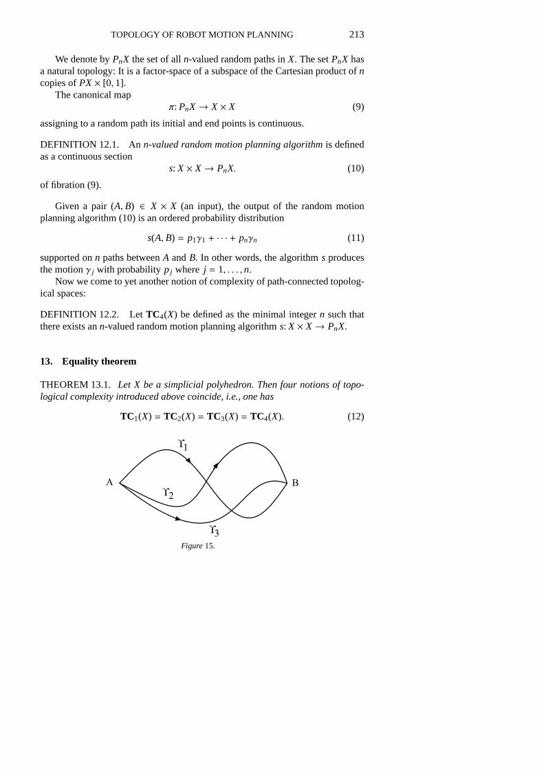
One thinks of the pathsγ1, . . . , γn as being differentstatesof σ (Figure 15).The numberp j is theprobability that the random pathσ is in stateγ j . Random

pathσ as above will be written as a formal linear combination

σ = p1γ1 + p2γ2 + · · · + pnγn.

Equality betweenn-valued random paths is understood as follows: the randompath

σ = p1γ1 + p2γ2 + · · · + pnγn.

is equal toσ′ = p′1γ

′1 + p′2γ

′2 + · · · + p′nγ

′n

iff p j = p′j for all j = 1, . . . ,n and, besides,γ j = γ′j for all indices j with p j , 0.In other words, the pathγ j which appears with the zero probabilityp j = 0

could be replaced by any other path starting atA and ending atB.

Figure14.


We denote byPnX the set of alln-valued random paths inX. The setPnX hasa natural topology: It is a factor-space of a subspace of the Cartesian product ofncopies ofPX× [0,1].

The canonical mapπ: PnX→ X × X (9)

assigning to a random path its initial and end points is continuous.

DEFINITION 12.1. Ann-valued random motion planning algorithmis definedas a continuous section

s: X × X→ PnX. (10)

of fibration (9).

Given a pair (A, B) ∈ X × X (an input), the output of the random motionplanning algorithm (10) is an ordered probability distribution

s(A, B) = p1γ1 + · · · + pnγn (11)

supported onn paths betweenA andB. In other words, the algorithms producesthe motionγ j with probability p j where j = 1, . . . ,n.

Now we come to yet another notion of complexity of path-connected topolog-ical spaces:

DEFINITION 12.2. LetTC4(X) be defined as the minimal integern such thatthere exists ann-valued random motion planning algorithms: X × X→ PnX.

13. Equality theorem

THEOREM 13.1. Let X be a simplicial polyhedron. Then four notions of topo-logical complexity introduced above coincide, i.e., one has

TC1(X) = TC2(X) = TC3(X) = TC4(X). (12)

Figure15.

214 M. FARBER

Proof.Let k denoteTC1(X) and lets: X×X→ PX be a tame motion planningalgorithm (as in Definition 7.1). We have a splittingX × X = F1 ∪ · · · ∪ Fk intodisjoint ENRs such that the restrictions|F j is continuous. Let us show that onemay enlarge each setF j to an open setU j ⊃ F j such that the sections|F j extendsto a continuous sections′j defined onU j . This would prove that

TC2(X) ≤ TC1(X). (13)

We will use the following property of the ENRs:If F ⊂ X and both spacesFandX are ENRs then there is an open neighborhoodU ⊂ X of F and a retractionr: U → F such that the inclusionj: U → X is homotopic toi ◦ r, wherei: F → Xdenotes the inclusion. See Dold, (1972, Chapter 4, Section 8) for a proof.

Using the fact that the setsFi andX × X are ENRs, we find that there existsan open neighborhoodUi ⊂ X × X of the setFi and a continuous homotopyhiτ: Ui → X×X, whereτ ∈ [0, 1], such thathi

0: Ui → X×X is the inclusion andhi1

is a retraction ofUi ontoFi . We will describe now a continuous maps′i : Ui → PXwith E ◦ s′i = 1Ui . Given a pair (A, B) ∈ Ui , the pathhi

τ(A, B) in X × X is a pairof paths (γ, δ), whereγ is a path inX starting at the pointγ(0) = A and endingat a pointγ(1), andδ is a path inX starting atB = δ(0) and ending atδ(1). Notethat the pair

(γ(1), δ(1)

)belongs toFi ; therefore the motion plannersi : Fi → PX

defines a pathξ = si

(γ(1), δ(1)

) ∈ PX

connecting the pointsγ(1) andδ(1). Now we sets′i (A, B) to be the concatenationof γ, ξ, andδ−1 (the reverse path ofδ):

s′i (A, B) = γ · ξ · δ−1.

Now we want to show thatX always admits a tame motion planning algorithm(see Definition 7.1) with the number of local domainsF j equal to` = TC2(X).This will show that

TC1(X) ≤ TC2(X). (14)

LetU1 ∪ U2 ∪ · · · ∪ U` = X × X, where` = TC2(X), (15)

be an open cover such that for anyi = 1, . . . , ` there exists a continuous motionplanning mapsi : Ui → PX with π ◦ si = 1Ui . Find a piecewise linear partitionof unity { f1, . . . , f`} subordinate to the cover (15). Herefi : X × X → [0, 1] is apiecewise linear function with support inUi and such that for any pair (A, B) ∈X × X, it holds that

f1(A, B) + f2(A, B) + · · · + f`(A, B) = 1.


Fix numbers 0< ci < 1 wherei = 1, . . . , ` with c1 + · · · + c` = 1. Let a subsetVi ⊂ X× X, wherei = 1, . . . , `, be defined by the following system of inequalities

{f j(A, B) < c j for all j < i,fi(A, B) ≥ ci .

Then:

(a) eachVi is an ENR;

(b) Vi is contained inUi ; therefore, the sectionsi : Ui → PX restricts ontoVi anddefines a continuous section overVi ;

(c) the setsVi are pairwise disjoint,Vi ∩ V j = ∅ for i , j;

(d) V1 ∪ V2 ∪ · · · ∪ Vk = X × X.

Hence we see that the setsVi and the sectionssi |Vi define a tame motionplanning algorithm in the sense of Definition 7.1 with` = TC2(X) local domains.

Now we prove thatTC3(X) ≤ TC2(X). (16)

Suppose thats: X×X→ PX is a tame motion planning algorithm with domains ofcontinuityF1, . . . , Fk ⊂ X×X. Denote the order of instability of the decompositionX × X = F1 ∪ · · · ∪ Fk by r ≤ k. Then any intersection of the form

F i1 ∩ · · · ∩ F ir+1 = ∅, (17)

is empty, where 1≤ i1 < i2 < · · · < ir+1 ≤ k. For any indexi = 1, . . . , k fixa continuous functionfi : X × X → [0,1] such thatfi(A, B) = 1 if and only ifthe pair (A, B) belongs toF i and such that the support supp(fi) retracts ontoFi .Let φ: X × X → R be the maximum of (finitely many) functions of the formfi1 + fi2 + · · · + fir+1 for all increasing sequences 1≤ i1 < i2 < · · · < ir+1 ≤ k oflengthr + 1. We have:

φ(A, B) < r + 1

for any pair (A, B) ∈ X × X, as follows from (17).Let Ui ⊂ X × X denote the set of all (A, B) such that

(r + 1) · fi(A, B) > φ(A, B).

Then Ui is open and containsF i , and hence the setsU1, . . . ,Uk form an opencover ofX × X. On the other hand, any intersection

Ui1 ∩ Ui2 ∩ · · · ∩ Uir+1 = ∅

is empty.As above we may assume that the setsU1, . . . ,Uk are small enough so that

over eachUi there exists a continuous motion planning section (here we use

216 M. FARBER

the assumption that eachFi is an ENR). Applying Lemma 13.2 (see below) weconclude thatTC2(X) ≤ r.

Combining inequalities (7), (13), (14), (16) we obtainTC1(X) = TC2(X) =

TC3(X).Next we show thatTC2(X) = TC4(X). This last argument is an adjustment of

the proof of Schwarz (1966, Proposition 2).Assume that there exists ann-valued random motion planning algorithms: X×

X→ PnX in X. The right-hand side of formula (11) defines continuous real valuedfunctions p j : X × X → [0, 1], where j = 1, . . . ,n. Let U j denote the open setp−1

j (0,1] ⊂ X × X. The setsU1, . . . ,Un form an open covering ofX × X. Settingsj(A, B) = γ j , one gets a continuous mapsj : U j → PX with π ◦ si = 1U j . Hence,n ≥ TC2(X) according to the definition ofTC2(X).

Conversely, settingk = TC2(X), we obtain that there exists an open coverU1, . . . ,Uk ⊂ X×X and a sequence of continuous mapssi : Ui → PXwhereπ◦si =

1Ui , i = 1, . . . , k. Extendsi to an arbitrary (possibly discontinuous) mapping

Si : X × X→ PX

satisfyingπ ◦ Si = 1X×X. This can be done without any difficulty; it amounts inmaking a choice of a connecting path for any pair of points (A, B) ∈ X×X−Ui . Onemay find a continuous partition of unity subordinate to the open coverU1, . . . ,Uk.It is a sequence of continuous functionsp1, . . . , pk: X × X → [0,1] such that forany pair (A, B) ∈ X × X one has

p1(A, B) + p2(A, B) + · · · + pk(A, B) = 1

and the closure of the setp−1i (0,1] is contained inUi . We obtain a continuousk-

valued random motion planning algorithms: X×X→ PnX given by the followingexplicit formula

s(A, B) = p1(A, B)S1(A, B) + · · · + pk(A, B)Sk(A, B). (18)

The continuity ofs follows from the continuity of the mapsSi restricted to thedomainsp−1

i (0, 1]. This completes the proof. ¤

LEMMA 13.2. Let X be a path-connected metric space. Consider an open coverX×X = U1∪U2∪ · · · ∪U` such that for anyi = 1, . . . , ` there exists a continuousmapsi : Ui → PXwithπ◦si = 1Ui . Suppose that for some integerr any intersection

Ui1 ∩ Ui2 ∩ . . . ∩ Uir = ∅

is empty where1 ≤ i1 < i2 < · · · < ir ≤ `. ThenTC2(X) < r.

A proof of Lemma 13.2 can be found in Farber (2004).


Although the numbersTC j(X) (where j = 1, 2, 3, 4) coincide whenX isa simplicial polyhedron, they do not coincide whenX is a general topologicalspace. The most convenient notion topologically isTC2(X).

Notation.In what follows we will use the notationTC(X) = TC2(X).

14. An upper bound for TC(X)

THEOREM 14.1. For any path-connected paracompact locally contractiblespaceX one has

TC(X) ≤ 2 dimX + 1, (19)

wheredimX denotes the covering dimension ofX.Proof. We know thatTC(X) ≤ cat(X × X). Combine this with cat(X × X) ≤

dim(X × X) + 1 = 2 dimX + 1. ¤

This result can be improved assuming thatX is highly connected:

THEOREM 14.2. If X is anr-connected CW-complex then

TC(X) <2 · dimX + 1

r + 1+ 1. (20)


15. A cohomological lower bound for TC(X)

In this section we describe a result from Farber (2003).Let k be a field. The cohomologyH∗(X;k) = H∗(X) is a gradedk-algebra

with the multiplication

∪: H∗(X) ⊗ H∗(X)→ H∗(X)

given by the cup-product. The tensor productH∗(X) ⊗ H∗(X) is again a gradedk-algebra with the multiplication

(u1 ⊗ v1) · (u2 ⊗ v2) = (−1)|v1|·|u2|u1u2 ⊗ v1v2.

Here|v1| and|u2| denote the degrees of cohomology classesv1 andu2 correspond-ingly. The cup-product∪ is an algebra homomorphism.

DEFINITION 15.1. The kernel of the homomorphism

∪: H∗(X) ⊗ H∗(X)→ H∗(X)

is called the ideal of the zero-divisors ofH∗(X). The zero-divisors-cup-length ofH∗(X) is the length of the longest nontrivial product in the ideal of the zero-divisors ofH∗(X).

218 M. FARBER

THEOREM 15.2. TC(X) is greater than the zero-divisors-cup-length ofH∗(X).


16. Examples

EXAMPLE 16.1. Consider the caseX = Sn. Let u ∈ Hn(Sn) be the fundamentalclass, and let 1∈ H0(Sn) be the unit. Then

a = 1⊗ u− u⊗ 1 ∈ H∗(Sn) ⊗ H∗(Sn)

is a zero-divisor. Another zero-divisor isb = u⊗ u. Computinga2 = a · a we find

a2 =((−1)n−1 − 1

) · u⊗ u.

Hencea2 = −2b for n even anda2 = 0 for n odd.We conclude:the zero-divisors-cup-length ofH∗(Sn;Q) equals1 for n odd

and 2 for n even. Applying Theorem 15.2 we find thatTC(Sn) ≥ 2 for n oddandTC(Sn) ≥ 3 for n even. In Section 7 we constructed explicit motion planningalgorithms having topological complexity 2 forn odd and 3 forn even. Hence,

TC(Sn) =

{2, if n is odd,3, if n is even.

EXAMPLE 16.2. Here we calculate the numberTC(X) whenX is a graph.

THEOREM 16.3. If X is a connected finite graph then

TC(X) =

1, if b1(X) = 0,2, if b1(X) = 1,3, if b1(X) > 1.

Proof. If b1(X) = 0 thenX is contractible and henceTC(X) = 1. If b1(X) = 1thenX is homotopy equivalent to the circle and thereforeTC(X) = TC(S1) = 2,see above. Assume now thatb1(X) > 1. Then there exist two linearly independentclassesu1,u2 ∈ H1(X). Thus

1⊗ ui − ui ⊗ 1, i = 1,2

are zero-divisors and their product equalsu2 ⊗ u1 − u1 ⊗ u2 , 0 which impliesTC(X) ≥ 3. On the other hand, we know thatTC(X) ≤ 3 by Theorem 14.1. Thiscompletes the proof. ¤

EXAMPLE 16.4. LetX = Σg be a compact orientable surface of genusg. Then

TC(X) =

{3, if g ≤ 1,5, if g > 1.

We leave the proof as an exercise.


17. Simultaneous control of many systems

Suppose that we have to control two systems simultaneously. We assume that thesystems do not interact, i.e., the admissible states of one of the systems do notdepend on the state of the other. LetX andY be the corresponding configurationspaces. If we view these two systems as a new single system then the configurationspace is the productX × Y. For the topological complexity of the product one hasthe inequality:

THEOREM 17.1. TC(X × Y) ≤ TC(X) + TC(Y) − 1.

A proof can be found in Farber (2003).Suppose now that one has to control simultaneouslyn systems having config-

uration spacesX1, . . . ,Xn. The total configuration space is the Cartesian product

Yn = X1 × X2 × . . . × Xn. (21)

We ask:What is the asymptotics of the topological complexityTC(Yn) for largen?

We shall assume that the topological complexity of the spaceXn is bounded,i.e., there exists a constantM ≥ 1 such thatTC(Xn) ≤ M for all n. ApplyingTheorem 17.1 one obtains the inequality

TC(Yn) ≤ n · [M − 1] + 1. (22)

This shows that the sequenceTC(Yn) growths at most linearly.Let us assume additionally that each spaceXn is path-connected andhomolog-

ically nontrivial, i.e.,H∗(Xn) , H∗(pt). Then one has

TC(Yn) ≥ n + 1. (23)Proof.Let ur ∈ Hir (Xr ) be a nontrivial class, whereir > 0. Denote

wr = 1× 1× · · · × ur × 1× · · · × 1 ∈ Hir (Yn)

(hereur stands on ther-th place). Then

n∏

j=1

w j ∈ H∗(Yn)

is a nonzero class. The class

w j = w j ⊗ 1− 1⊗ w j , j = 1, . . . ,n

is a zero-divisor and the product

n∏

j=1

w j =

( n∏

j=1

w j

)⊗ 1± . . . , 0

220 M. FARBER

is nonzero. This proves (22) as follows from the cohomological lower bound.¤

Combining the inequalities (22) and (23) one obtains:

COROLLARY 17.2. Assume that each spaceXr is path-connected and homolog-ically nontrivial and the topological complexityTC(Xr ) is bounded above. Thenthe topological complexity of the productYn (see(21)) (viewed as a function ofn)has a linear growth. In particular, for any finite-dimensional path-connected andhomologically nontrivial polyhedronX the sequenceTC(Xn) as a function ofnhas a linear growth.

This result has an important implication in the control theory:

THEOREM 17.3. A centralized control byn identical independent systems hastopological complexity which is linear inn (more precisely, the inequalities(22)and (23) are satisfied). The distributed control, i.e., when each of the objects iscontrolled independently of the others, has an exponential topological complexityTC(X)n.

We see that in practical situations the centralized control by many independentobjects could be organized so that its “much more stable” than the distributedcontrol.

18. Another inequality relating TC(X) to the usual category

The result of this section was inspired by a discussion with H.-J. Baues.Consider the fibrationπ: PX→ X × X, cf. Definition 6.1.

LEMMA 18.1. Let U ⊂ X × X be a subset. There exists a continuous sections: U → PX, π ◦ s = 1U of π over U if and only if the inclusionU → X × X ishomotopic to a map with values in the diagonal∆X ⊂ X × X.

Proof. Let s: U → PX be a section. Heres(A, B)(t) ∈ X is a continuousfunction of A, B, t (where (A, B) ∈ U and t ∈ [0,1]) such thats(A, B)(0) = Aands(A, B)(1) = B. Define

σ: U × [0,1]→ X × X

byσ(A, B)(t) = (s(A, B)(t), B). Then one hasσ(A, B)(0) = (A, B) andσ(A, B)(1) =

(B, B) takes values on the diagonal∆X. Henceσ is a homotopy between theinclusionU → X × X and a map with values on the diagonal.

Conversely, suppose thatσt: U → X × X is a homotopy from the inclusion toa map with values on the diagonal. Thent 7→ σt(A, B) is a path inX × X whichstarts at (A, B) and ends at a point (C,C). In other words,σt(A, B) is a pair (γ1, γ2)


of paths inX whereγ1 starts atA, γ2 starts atB, and the end points of these pathscoincide. Hence the paths = γ1γ

−12 ∈ PX is well-defined, continuously depends

on A and B and starts atA and ends atB. We obtain a continuous section ofπoverU. ¤

COROLLARY 18.2. The topological complexityTC(X) is the smallestk suchthat X×X can be covered byk open subsetsU1∪U2∪ · · · ∪Uk = X×X such thateachU j → X×X is homotopic to a map with values in the diagonal∆X ⊂ X×X.

The following inequality complements Lemma 9.2.

LEMMA 18.3. If X is an ENR then

TC(X) ≥ cat((X × X)/∆X

) − 1.Proof. Let X × X = U1 ∪ U2 ∪ · · · ∪ Uk and eachUi → X × X is homotopic

to a map with values in∆(X). Let U′j = U j − ∆(X) andU′′j ⊂ (X × X)/∆(X) bethe image ofU′j under the canonical mapX × X → X × X/∆X. ThenU′′j is null-homotopic and these sets cover the wholeX × X/∆X except the base point of thefactor-space. Hence, adding a contractible neighborhood of the base point givesa categorical cover of the factor-space. Existence of such neighborhood followsfrom the ENR assumption. This completes the proof. ¤

19. Topological complexity of bouquets

It is quite obvious that

TC(X ∨ Y) ≥ max{TC(X),TC(Y)}. (24)

We shall prove the following:

THEOREM 19.1. Let X andY be two polyhedrons. ThenTC(X ∨ Y) is less thanor equal to

max{TC(X),TC(Y), cat(X) + cat(Y) − 1}. (25)Proof.The product (X ∨ Y) × (X ∨ Y) is a union of four spaces

X × X, Y× Y, X × Y, Y× X

and any two of these spaces intersect at a single point (p, p) wherep is the joinpoint of the wedgeX ∨ Y. Over each of these sets one may construct a motionplanning algorithm having respectively

TC(X), TC(Y), cat(X) + cat(Y) − 1, cat(X) + cat(Y) − 1

222 M. FARBER

domains of continuity. For example, the algorithm overX × Y takes pairs (x, y) ∈X × Y as an input and finds a pathα in X connectingx with p, a pathβ in Yconnectingy with p and finally produces the pathαβ−1 as the output. To makethe choice ofα continuous one has to splitX into cat(X) pieces; to make thechoice ofβ continuous one splitsY into cat(Y) pieces. Similarly to the proof of theproduct inequality (see Farber, 2003, Theorem 11) one may rearrange the totalityof cat(X) × cat(Y) products into cat(X) + cat(Y) − 1 sets (the checkerboard trick)such that the algorithm is continuous over each of them.

The remaining arguments of the proof are similar (compare with the nextsection), we leave them as an exercise for the reader. ¤

20. A general recipe to construct a motion planning algorithm

Let X be a path-connected polyhedron and letU = {U1,U2, . . . ,Un} be aniceopen cover ofX with the property that each inclusionUi → X is null-homotopic.The word “nice” means that the Main assumption (see below) is satisfied. Ourgoal isto construct a motion planning algorithm inX with 2m− 1 local domainswheremis the multiplicity of the coveringU, i.e., the maximal number of distinctdomainsU j having a nonempty intersection.

Introduce subsetsV1, V2, . . . ,Vm whereVr ⊂ X denotes the set of pointsx ∈ Xwhich are covered by preciselyr setsU j .

Main assumption.EachVi is an ENR.

For any multi-indexα = (1 ≤ i1 < i2 < · · · < ir ≤ n) denote

Uα =

r⋂

k=1

Uik.

ThenVr =

⋃

|α|=r

Uα −⋃

|α|=r+1

Uα. (26)

Note thatVr = ∅ for r > m.

LEMMA 20.1.

(A) Each setWα = Uα ∩ Vr (where|α| = r) is closed and open inVr .

(B) The setsWα andWβ are disjoint forα , β, |α| = r = |β|.


Proof.Clearlyx ∈ Uα ∩Uβ implies thatx ∈ Uα∪β. This implies statement (B).Now we want to show slightly more, namely, that the setsWα and Wβ are

disjoint for |α| = r = |β|, α , β. Indeed, if x ∈ Wα ∩ Wβ then x = lim xn

wherexn ∈ Wα. Sincex lies in Wβ one hasxn ∈ Wβ for all largen and hencexn ∈ Uα∪β 1 Vr — a contradiction.

These two statements imply thatWα ∩ Vr = Wα i.e., Wα is closed inVr . Asfollows from the definitionWα is also open inVr . ¤

LEMMA 20.2. One hasVr ⊂

⋃

k≤r

Vk. (27)

Proof. It follows directly from (26). ¤

LEMMA 20.3. Over each setVr × Vr ′ ⊂ X × X one may construct an explicitcontinuous section of the fibrationπ: PX→ X × X.

Proof. We know thatVr =⋃|α|=k Wα and eachWα is open and closed inVr .

Hence it is enough to construct a continuous section over eachWα ×Wβ. Let i andj be the smallest indices appearing in the multi-indicesα andβ correspondingly.Then Wα ⊂ Ui and Wβ ⊂ U j . Let Hi

t : Ui × I → X and H jt : U j × I → X be

the homotopies contractingUi andU j to the base pointx0 ∈ X. Then, given apair (x, y) ∈ Wα × Wβ one constructs a path connecting them as follows: it isconcatenation of the pathHi

t(x) leading fromx to the base point and then followsthe reverse path toH j

t (y). ¤

DenoteAk =

⋃

r+r ′=k+1

Vr × Vr ′ ⊂ X × X, (28)

wherek = 1, 2, . . . ,2m− 1. These sets are ENR’s (by the assumption) and coverX × X.

LEMMA 20.4. Each productVr × Vr ′ , wherer + r ′ = k + 1, is closed and openin Ak.

Proof. It follows from (20.2). ¤

Hence the described above local sections over eachVr × Vr ′ combine into acontinuous section overAk. In total, we have 2m− 1 local sections.

21. How difficult is to avoid collisions inRm?

In this section we start discussing the problem of finding the topological complex-ity TC

(F(Rm,n)

)of the configuration spaceF(Rm,n) of n distinct points in the

224 M. FARBER

Euclidean spaceRm. A motion planning algorithm inF(Rm,n) takes as an inputtwo configurations ofn distinct points inRm and producesn continuous curvesA1(t), . . . ,An(t) ∈ Rm, wheret ∈ [0, 1], such thatAi(t) , A j(t) for all t ∈ [0,1],i , j and

(A1(0), . . . ,An(0)

)and

(A1(1), . . . ,An(1)

)are the first and the second

given configurations. In other words, a motion planning algorithm inF(Rm,n)moves one of the given configurations into another avoiding collisions.

The following theorem was obtained in Farber and Yuzvinsky (2004).

THEOREM 21.1. One has

TC(F(Rm,n)) =

{2n− 1 for any oddm,2n− 2 for m = 2.

At the moment we do not know the answer for the casem≥ 4 even. We knowthat in this case the numberTC(F(Rm,n)) is either 2n− 1 or 2n− 2.

Conjecture. For anymeven one hasTC(F(Rm, n)) = 2n− 2.

We will give here some ideas of the proof of Theorem 21.1 referring the readerto Farber and Yuzvinsky (2004) for details. We will also discuss the possibleapproaches to construct explicit motion planning algorithms inF(Rm, n). Suchalgorithms could be useful in situations when a large number of objects must bemoved automatically (without human intervention) from one position to anotheravoiding collisions.

Consider the set

Hi j = {(y1, . . . , yn); yi ∈ Rm, yi = y j} ⊂ Rnm.

Herei, j ∈ {1, 2, . . . ,n}, i < j. The setHi j is a linear subspace ofRnm of codimen-sionm. The system of subspaces{Hi j }i< j is an arrangement of linear subspaces ofcodimensionm. Our approach to the problem is to view the union

H =⋃

i< j

Hi j

as the set of obstacles:F(Rm,n) = Rnm− H.

22. The casem = 2

Assume first thatm = 2. This means that we are dealing withn distinct particleson the plane. ThenHi j ⊂ Cn is a complex subspace of codimension 1.


Consider a slightly more general situation. LetA = {H} be a finite set ofhyperplanes in an affine complex spaceCn. Denote byM(A) the complement

M(A) = Cn −⋃

H∈AH.

We will study the motion planning problem inM(A). We may say that we live inCn and the union of hyperplanes

⋃H represent our obstacles.

Recall some terminology from the theory of arrangements (Orlik and Terao,1992). If

⋂H∈A H , ∅ thenA is calledcentral, and up to change of coordinates

the hyperplanes can be assumed linear. Suppose thatA is linear. For eachH ∈ Aone can fix a linear functionalαH (unique up to a non-zero multiplicative constant)such thatH = {αH = 0}. A set of hyperplanesHi ∈ A is calledlinear independentif the corresponding functionalsαHi are linearly independent. The rank of{αH},i.e., the cardinality of a maximal independent subset, is called therank of Aand denoted by rk(A). Clearly rk(A) ≤ n and the equality occurs if and onlyif

⋂H H = 0.If A is not central we define its rank as the rank of a maximal central subar-

rangement ofA.While dealing with the arrangement complements we will need the following

nontrivial result (Orlik and Terao, 1992):if A is an arbitrary arrangement ofrank r then the complementM(A) has homotopy type of a simplicial complex ofdimensionr.

Note that the rank of the braid arrangement{Hi j }i< j in Cn equalsn− 1.

COROLLARY 22.1. The configuration spaceF(C,n) has homotopy type of asimplicial complex of dimensionn− 1.

Combining this with Theorems 10.1 and 14.1 we obtain:

COROLLARY 22.2. TC(F(C,n)

) ≤ 2n− 1.

This result can be improved:

THEOREM 22.3. LetA be a central complex hyperplane arrangement of rankr. Then the topological complexity of the complementM(A) is less or equal than2r. In particular one hasTC

(F(C, n)

) ≤ 2n− 2.Proof.LetA be{H1, . . . ,H`} ⊂ Cn. Let H∗1 be a parallel copy ofH1 which is

disjoint fromH1. Then the intersections

Hi ∩ H∗1, i = 2, 3, . . . , `

form a (in general, non-central) hyperplane arrangementA∗ in H∗1 ' Cn−1 of rankr − 1. There is a principalC∗-fibrationM(A)→ M(A∗). The inclusionM(A∗) ⊂

226 M. FARBER

M(A) is a section of it. Hence the fibration is trivialM(A) ' M(A∗) × C∗ andusing the product inequality (see Theorem 17.1) we find

TC(M(A)) ≤ TC(M(A∗)) + TC(C∗) − 1

≤ [2(r − 1) + 1] + 2− 1 = 2r. ¤

The opposite inequality requires an additional geometric property of the ar-rangement:

THEOREM 22.4. LetA be a complex central hyperplane arrangement of rankr. Assume that there exist2r − 1 hyperplanesH1,H2, . . . ,H2r−1 such thatH1,H2, . . . ,Hr are independent and for any1 ≤ j ≤ r the hyperplanesH j , Hr+1,Hr+2, . . . ,H2r−1 are independent. Then one hasTC

(M(A)

) ≥ 2r.

The proof (see Farber and Yuzvinsky, 2004) uses the cohomological lowerbound for the topological complexity and combinatorics of Orlik – Solomon alge-bras.

EXAMPLE 22.5. Consider the braid arrangement{Hi j }i< j ⊂ Cn. Herer = n− 1and 2r − 1 = 2n− 3. We have 2n− 3 hyperplanes:

H12,H13, . . . ,H1n,H23,H24, . . . ,H2n

satisfying the condition of the above theorem.

COROLLARY 22.6. One hasTC(F(R2, n)

)= 2n− 2.

23. TC(F(Rm, n)

)in the casem ≥ 3 odd

Assume thatm ≥ 3 is odd. ThenF(Rm,n) is (m− 2)-connected and in particularit is simply connected. Its cohomology algebra is generated by the cohomologyclasses

ei j ∈ Hm−1(F(Rm, n)), i , j

which arise as follows. Consider the map

φi j : F(Rm, n)→ Sm−1, (y1, y2, . . . , yn) 7→ yi − y j

|yi − y j | ∈ Sm−1.

Thenei j = φ∗i j [S

m−1]

where [Sm−1] is the fundamental class of the sphereSm−1.


The cohomology classesei j satisfy the following relations:

e2i j = 0, and ei j ejk + ejkeki + ekiei j = 0 (29)

for any triple i, j, k. It follows that a productei1 j1ei2 j2 · · · eik jk is nonzero if andonly if the subgraph of the full graph on vertices{1,2, . . . ,n} having the edges(ir , jr ) contains no cycles.

Hence form ≥ 3 the configuration spaceF(Rm,n) has homotopy type of apolyhedron of dimension≤ (n− 1)(m− 1). Since it is (m− 2)-connected we mayuse inequality (20) of Theorem 14.2 to find

TC(F(Rm, n)) <2(n− 1)(m− 1) + 1

m− 1+ 1 = 2n− 1 +

1m− 1

.

We obtain:

COROLLARY 23.1. TC(F(Rm, n)

) ≤ 2n− 1.

We want to show that an equality holds in Corollary!23.1. We shall use thecohomological lower bound (see Theorem 15.2). Set ¯ei j = 1⊗ ei j − ei j ⊗ 1. It is azero-divisor of the cohomology algebra. Note that (¯ei j )2 = −2 · ei j ⊗ ei j , 0. Herewe use the assumption thatm is odd.

Consider the following product

π =

n∏

i=2

(e1i)2 ∈ A⊗ A.

We findπ = (−2)n−1m⊗m, where

m =

n∏

i=2

e1i .

The monomialm, 0 is nonzero and hence the productπ is nonzero.Using the cohomological lower bound for the topological complexity we ob-

tain the opposite inequalityTC(M) ≥ 2n− 1. This completes the proof of Theo-rem 21.1 in the casem≥ 3 odd.

24. Shade

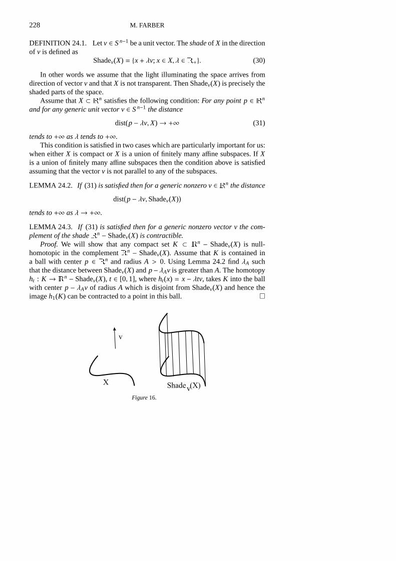
Let X ⊂ Rn be a closed subset with connected complementRn − X. Our purposeis to find (or to estimate) the numberTC(Rn − X). Our main motivation is thespecial case whenX = ∪H is the union of finitely many affine subspaces.

228 M. FARBER

DEFINITION 24.1. Letv ∈ Sn−1 be a unit vector. Theshadeof X in the directionof v is defined as

Shadev(X) = {x + λv; x ∈ X, λ ∈ R+}. (30)

In other words we assume that the light illuminating the space arrives fromdirection of vectorv and thatX is not transparent. Then Shadev(X) is precisely theshaded parts of the space.

Assume thatX ⊂ Rn satisfies the following condition:For any pointp ∈ Rn

and for any generic unit vectorv ∈ Sn−1 the distance

dist(p− λv,X)→ +∞ (31)

tends to+∞ asλ tends to+∞.This condition is satisfied in two cases which are particularly important for us:

when eitherX is compact orX is a union of finitely many affine subspaces. IfXis a union of finitely many affine subspaces then the condition above is satisfiedassuming that the vectorv is not parallel to any of the subspaces.

LEMMA 24.2. If (31) is satisfied then for a generic nonzerov ∈ Rn the distance

dist(p− λv,Shadev(X)

)

tends to+∞ asλ→ +∞.

LEMMA 24.3. If (31) is satisfied then for a generic nonzero vectorv the com-plement of the shadeRn − Shadev(X) is contractible.

Proof. We will show that any compact setK ⊂ Rn − Shadev(X) is null-homotopic in the complementRn − Shadev(X). Assume thatK is contained ina ball with centerp ∈ Rn and radiusA > 0. Using Lemma 24.2 findλA suchthat the distance between Shadev(X) andp− λAv is greater thanA. The homotopyht : K → Rn − Shadev(X), t ∈ [0, 1], whereht(x) = x− λtv, takesK into the ballwith centerp − λAv of radiusA which is disjoint from Shadev(X) and hence theimageh1(K) can be contracted to a point in this ball. ¤

Figure16.


DEFINITION 24.4. LetX ⊂ Rn be a closed subset satisfying (31). The shadingdimension ofX is defined as the smallestr such that there exist unit vectorsv1, . . . , vr+1 such that the intersection

r+1⋂

i=1

Shadevi (X) = X (32)

equalsX. Equivalently,r + 1 is the minimal number of projectors (placed atinfinity) needed to illuminate the spaceRn − X.

EXAMPLE 24.5. LetX ⊂ Rn be a finite setX = {p1, . . . , pm} then its shadingdimension is 1. Indeed, choose a generic unit vectoru ∈ Sn−1 such that no linethroughpi andp j has directionu. Thenu and−u are two directions such that theintersection of their shades equalsX. Any line inRn in the direction ofu intersectsX in at most one point and hence the unit vectorsu and−u illuminate the wholecomplementRn − X.

THEOREM 24.6. If X ⊂ Rn is closed subset satisfying(31) then for the topolog-ical complexity of the complementTC(Rn − X) one has

TC(Rn − X) ≤ 2r + 1

wherer is the shading dimension ofX. Moreover, using the discussion of Sec-tion 20one obtains an explicit motion planning algorithm inRn−X with ≤ 2r +1local rules.

Proof. It follows from the results described above, since

Rn − X =

r+1⋃

i=1

(Rn − Shadevi (X)

)

and each termRn − Shadevi (X) is contractible. ¤

25. Illuminating the complement of the braid arrangement

Considern particles inRm which are disjoint from each other. In this case theobstacle setX ∈ Rm×Rm× · · · ×Rm = Rmn is

X =⋃

i< j

Hi j

whereHi j is the linear subspacezi = zj , i.e., the particle numberi collides withthe particle numberj.

230 M. FARBER

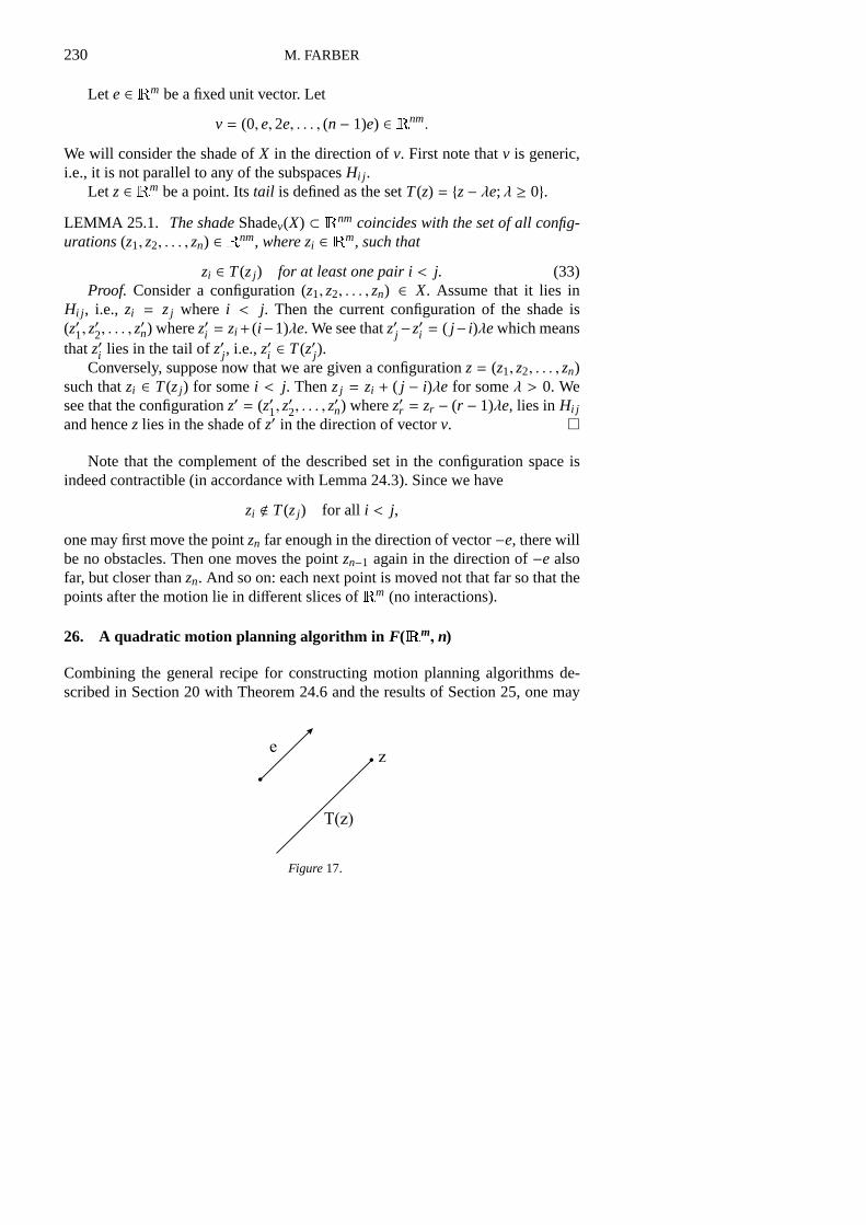
Let e ∈ Rm be a fixed unit vector. Let

v = (0,e, 2e, . . . , (n− 1)e) ∈ Rnm.

We will consider the shade ofX in the direction ofv. First note thatv is generic,i.e., it is not parallel to any of the subspacesHi j .

Let z ∈ Rm be a point. Itstail is defined as the setT(z) = {z− λe; λ ≥ 0}.LEMMA 25.1. The shadeShadev(X) ⊂ Rnm coincides with the set of all config-urations(z1, z2, . . . , zn) ∈ Rnm, wherezi ∈ Rm, such that

zi ∈ T(zj) for at least one pairi < j. (33)Proof. Consider a configuration (z1, z2, . . . , zn) ∈ X. Assume that it lies in

Hi j , i.e., zi = zj where i < j. Then the current configuration of the shade is(z′1, z

′2, . . . , z

′n) wherez′i = zi + (i−1)λe. We see thatz′j −z′i = ( j− i)λewhich means

thatz′i lies in the tail ofz′j , i.e.,z′i ∈ T(z′j).Conversely, suppose now that we are given a configurationz = (z1, z2, . . . , zn)

such thatzi ∈ T(zj) for somei < j. Thenzj = zi + ( j − i)λe for someλ > 0. Wesee that the configurationz′ = (z′1, z

′2, . . . , z

′n) wherez′r = zr − (r − 1)λe, lies inHi j

and hencez lies in the shade ofz′ in the direction of vectorv. ¤

Note that the complement of the described set in the configuration space isindeed contractible (in accordance with Lemma 24.3). Since we have

zi < T(zj) for all i < j,

one may first move the pointzn far enough in the direction of vector−e, there willbe no obstacles. Then one moves the pointzn−1 again in the direction of−e alsofar, but closer thanzn. And so on: each next point is moved not that far so that thepoints after the motion lie in different slices ofRm (no interactions).

26. A quadratic motion planning algorithm in F(Rm, n)

Combining the general recipe for constructing motion planning algorithms de-scribed in Section 20 with Theorem 24.6 and the results of Section 25, one may

Figure17.


construct an explicit motion planning algorithm with≤ n2 local rules wheren isthe number of particles. In this section we briefly explain how such algorithm canbe built.

Fix distinct unit vectorse1, e2, . . . ,eN ∈ Rm, where

N =n(n− 1)

2+ 1.

Then for any configurationz = (z1, . . . , zn) ∈ F(Rm, n) wherezi , zj , zi ∈ Rm,there exists 1≤ r ≤ N such that the vectorer (one of theN fixed unit vectors) isdistinct from all vectors

zi − zj

|zi − zj | , for all i < j.

Therefore the configurationz lies in the complement of the shade

Rnm− Shadeer (X).

HenceN contractible setsRnm − Shadeer (X), where r = 1, . . . ,N, cover thecomplementRnm − X. By the construction of Section 20 this leads to a motionplanning algorithm with

2N − 1 = n2 − n + 1

local rules.

27. Configuration spaces of graphs

Here we will discuss the configuration spacesF(Γ, n) whereΓ is a connectedgraph. These spaces were studied by Ghrist (2001), Ghrist and Koditschek (2002)and Abrams (2002); see also Gal (2001),Swia↪tkowski (2001). To illustrate theimportance of these configuration spaces for robotics one may mention the controlproblems where a number of automated guided vehicles (AGV) have to movealong a network of floor wires. The motion of the vehicles must be safe: it shouldbe organized so that the collisions do not occur. Ifn is the number of AGV thenthe natural configuration space of this problem isF(Γ,n) whereΓ is a graph.

The first question to ask is whether the configuration spaceF(Γ, n) is con-nected. ClearlyF(Γ,n) is disconnected ifΓ = [0,1] is a closed interval (andn ≥ 2)or if Γ = S1 is the circle andn ≥ 3. These are the only examples of this kind asthe following simple lemma claims:

LEMMA 27.1. Let Γ be a connected finite graph having at least one essentialvertex. Then the configuration spaceF(Γ, n) is connected.

An essential vertex is a vertex which is incident to 3 or more edges.

232 M. FARBER

Figure18.

THEOREM 27.2. Let Γ be a connected graph having an essential vertex. Thenthe topological complexity ofF(Γ, n) satisfies

TC(F(Γ,n)

) ≤ 2m(Γ) + 1, (34)

wherem(Γ) denotes the number of essential vertices inΓ.

A proof can be found in Farber (2005).

THEOREM 27.3. Let Γ be a tree having an essential vertex. Letn be an integersatisfyingn ≥ 2m(Γ) wherem(Γ) denotes the number of essential vertices ofΓ. Inthe casen = 2 we will additionally assume that the treeΓ is not homeomorphicto the letterY viewed as a subset of the planeR2. Then the upper bound(34) isexact, i.e.,

TC(F(Γ,n)

)= 2m(Γ) + 1. (35)

Farber (2005) contains a sketch of the proof and also an explicit description ofa motion planning algorithm inF(Γ,n) (assuming thatΓ is a tree) having precisely2m(Γ) + 1 domains of continuity.

If Γ is homeomorphic to the letterY thenm(Γ) = 1 andF(Γ, 2) is homotopyequivalent to the circleS1. Hence in this caseTC(F(Γ,2)) = 2. The equality (35)fails in this case.

For any treeΓ one hasTC(F(Γ,2)

)= 3 assuming thatΓ is not homeomorphic

to the letterY. This shows that the assumptionn ≥ 2m(Γ) of Theorem 27.3 cannotbe removed: ifΓ is a tree withm(Γ) ≥ 2 then the inequality above would giveTC

(F(Γ,2)

)= 2m(Γ) + 1 ≥ 5.

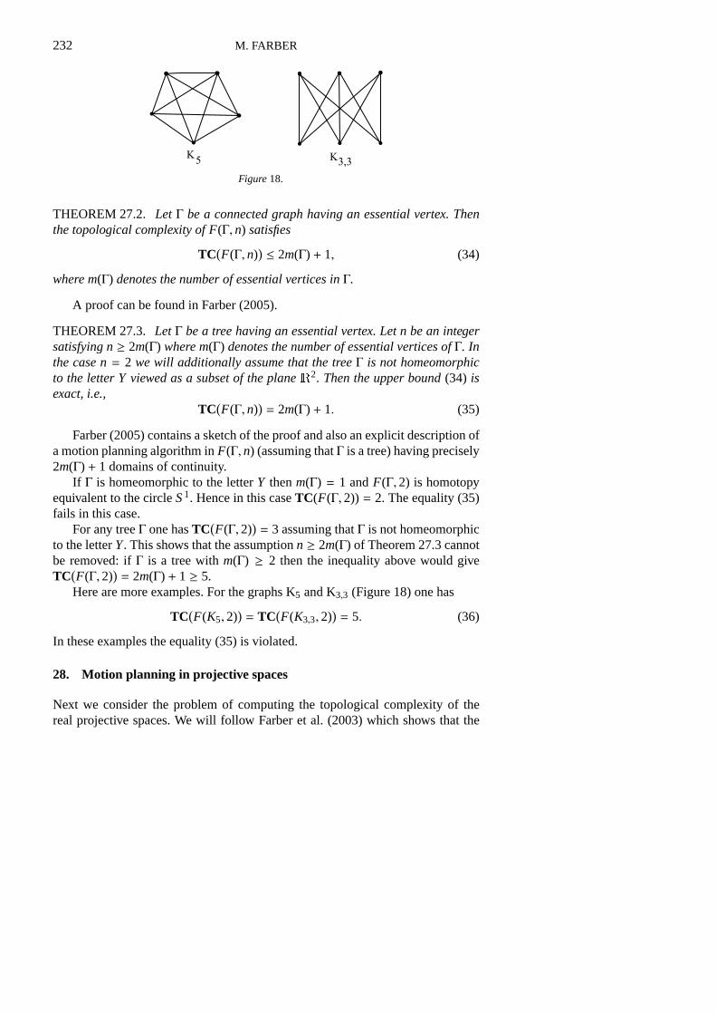
Here are more examples. For the graphs K5 and K3,3 (Figure 18) one has

TC(F(K5,2)

)= TC

(F(K3,3,2)

)= 5. (36)

In these examples the equality (35) is violated.

28. Motion planning in projective spaces

Next we consider the problem of computing the topological complexity of thereal projective spaces. We will follow Farber et al. (2003) which shows that the


Figure19.

problem of computing the numberTC(RPn) is equivalent to a classical problemof manifold topology which asks what is the minimal dimension of the EuclideanspaceN such that there exists an immersionRPn → RN. The immersion prob-lem for the real projective spaces was studied by many people and a variety ofimportant results was obtained. However at the moment the immersion dimensionofRPn as a function ofn is not known. We refer to a recent survey (Davis, 1993).

The problem of finding motion planning algorithms in the projective spaceRPn can be viewed as an elementary problem of topological robotics. Indeed,points ofRPn represent lines through the origin in the Euclidean spaceRn+1 andhence a motion planning algorithm inRPn should describe how a given lineA inRn+1 should be moved to another prescribed positionB.

Lines through the origin inR3 may represent metallic bars fixed at the fixedpoint by a revolving joint; this situation is common in the practical robotics.

If the angle between the linesA andB is acute then one may rotateA towardB in the two-dimensional plane spanned byA andB such thatA sweeps the acuteangle. Hence the problem reduces immediately to the special case when the linesA andB are orthogonal. In this case, if the intention is to use simple rotations, oneneeds a continuous choice of the direction of rotation in the plane spanned byAandB.

Note that the Lusternik – Schnirelmann category of the real projective spacesis well known and easy to compute: cat(RPn) = n+1. Using the general propertiesof the topological complexity mentioned above we may write

n + 1 ≤ TC(RPn) ≤ 2n + 1.

We shall see below (see Corollary 30.4) that in factTC(RPn) ≤ 2n for all n; theequality holds ifn is a power of 2.

The answer in the complex case is much simpler:

LEMMA 28.1. TC(CPn) = 2n + 1. More generally, for any simply connectedsymplectic manifoldM one has

TC(M) = dim M + 1.

234 M. FARBER

Proof. Let u ∈ H2(M) be the class of the symplectic form. We have a zero-divisoru⊗ 1− 1⊗ u satisfying

(u⊗ 1− 1⊗ u)2n = (−1)n(2nn

)un ⊗ un

where 2n = dim M. The cohomological lower bound givesTC(M) ≥ 2n + 1.The cohomological upper bound of Farber (2004) (using the assumption thatM issimply connected) gives the opposite inequalityTC(M) ≤ 2n + 1. ¤

THEOREM 28.2. If n ≥ 2r−1 thenTC(RPn) ≥ 2r .Proof. Let α ∈ H1(RPn;Z2) be the generator. The classα × 1 + 1 × α is a

zero-divisor. Consider the power

(α × 1 + 1× α)2r−1.

Assuming that 2r−1 ≤ n < 2r it contains the nonzero term(2r − 1

n

)αk ⊗ αn

wherek = 2r − 1 − n < n. Applying the cohomological lower bound the resultfollows. ¤

29. Nonsingular maps

The main result concerningTC(RPn) (see Theorem 29.2) uses the followingclassical notion:

DEFINITION 29.1. A continuous map

f :Rn ×Rn→ Rk (37)

is called nonsingular if:

(a) f (λu, µv) = λµ f (u, v) for all u, v ∈ Rn, λ, µ ∈ R, and

(b) f (u, v) = 0 implies that eitheru = 0, orv = 0.

In the mathematical literature there exist several variations of the notion of anonsingular map. We refer to Lam (1967) and Milgram (1967) where nonsingularmaps (of a different type) were used to construct immersions of real projectivespaces into the Euclidean space.

Problem.Givenn find the smallestk such that there exists a nonsingular mapf :Rn ×Rn→ Rk.


Let us show that for anyn there exists a nonsingular mapf :Rn×Rn→ R2n−1.Fix a sequenceα1, α2, . . . , α2n−1:Rn→ R of linear functionals such that anyn ofthem are linearly independent. Foru, v ∈ Rn the valuef (u, v) ∈ R2n−1 is definedas the vector whosejth coordinate equals the productα j(u)α j(v), where j = 1,2, . . . ,2n− 1. If u , 0 then at leastn among the numbersα1(u), . . . , α2n−1(u) arenonzero. Hence ifu , 0 andv , 0 there existsj such thatα j(u)α j(v) , 0 and thusf (u, v) , 0 ∈ R2n−1.

Remarks.

1. Fork < n there exist no nonsingular mapsf :Rn×Rn→ Rk (as follows fromthe Borsuk – Ulam theorem).

2. Forn = 1, 2, 4, 8 there exist nonsingular mapsf :Rn ×Rn → Rn having anadditional property that for anyu ∈ Rn, u , 0 the first coordinate off (u,u) ispositive.These maps use the multiplication of the real numbers, the complex numbers,the quaternions, and the Cayley numbers, correspondingly.

3. Forn distinct from 1, 2, 4, 8 there exist no nonsingular mapsf :Rn×Rn→ Rn

(as follows from the famous theorem of J. F. Adams).

Here is the main theorem of Farber et al. (2003):

THEOREM 29.2. The numberTC(RPn) coincides with the smallest integerksuch that there exists a nonsingular mapRn+1 ×Rn+1→ Rk.

We refer to Farber et al. (2003) for the proof. Here we will only explain(following Farber et al., 2003) how one uses the nonsingular maps to constructmotion planning algorithms.

PROPOSITION 29.3.If there exists a nonsingular mapRn+1×Rn+1→ Rk withn+1 < k thenRPn admits a motion planner withk local rules, i.e.,TC(RPn) ≤ k.

Proof.Let Φ:Rn+1×Rn+1→ R be a scalar continuous map such thatφ(λu, µv)= λµφ(u, v) for all u, v ∈ V andλ, µ ∈ R. Let Uφ ⊂ RPn ×RPn denote the set ofall pairs (A, B) of lines inRn+1 such thatA , B andφ(u, v) , 0 for some pointsu ∈ A andv ∈ B. It is clear thatUφ is open.

There exists a continuous maps defined onUφ with values in the space ofcontinuous paths in the projective spaceRPn such that for any pair (A, B) ∈ Uφ

the paths(A, B)(t), t ∈ [0,1], starts atA and ends atB. One may find unit vectorsu ∈ A andv ∈ B such thatφ(u, v) > 0. Such pairu, v is not unique: instead ofu,v we may take−u, −v. Note that both pairsu, v and−u, −v determine the sameorientation of the plane spanned byA, B. The desired mapsconsists in rotatingAtowardB in this plane, in the positive direction determined by the orientation.

236 M. FARBER

Assume now additionally thatφ:Rn+1×Rn+1→ R is positivein the followingsense: for anyu ∈ Rn+1, u , 0, one hasφ(u,u) > 0. Then instead ofUφ we maytake a slightly larger setU′φ ⊂ RPn ×RPn, which is defined as the set of all pairs

of lines (A, B) in Rn+1 such thatφ(u, v) , 0 for someu ∈ A andv ∈ B. Now allpairs of lines of the form (A,A) belong toU′φ. For A , B the path fromA to Bis defined as above (rotatingA towardB in the plane, spanned byA andB, in thepositive direction determined by the orientation), and forA = B we choose theconstant path atA. Then continuity is not violated.

A vector-valued nonsingular mapf :Rn+1 ×Rn+1 → Rk determinesk scalarmapsφ1, . . . , φk:Rn+1 × Rn+1 → R (the coordinates) and the described aboveneighborhoodsUφi cover the productRPn×RPn minus the diagonal. Sincen + 1< k one may replace the initial nonsingular map by such anf that for anyu ∈Rn+1, u , 0, the first coordinateφ1(u,u) of f (u,u) is positive. Now, the open setsU′φ1

, Uφ2, . . . ,Uφk coverRPn×RPn. We have described explicit motion planningstrategies over each of these sets. ThereforeTC(RPn) ≤ k.

30. TC(RPn) and the immersion problem

THEOREM 30.1. For anyn , 1, 3, 7 the numberTC(RPn) equals the smallestk such that the projective spaceRPn admits an immersion intoRk−1.

The proof (see Farber et al., 2003) uses Theorem 29.2 and the followingtheorem of Adem et al. (1972):

THEOREM 30.2. There exists an immersionRPn → Rk (wherek > n) if andonly if there exists a nonsingular mapRn+1 ×Rn+1→ Rk+1.

We will give here a direct construction of a motion planning algorithm inRPn

starting from an immersionRPn→ Rk.

THEOREM 30.3. Suppose that the projective spaceRPn can be immersed intoRk. ThenTC(RPn) ≤ k + 1.

Proof. ImagineRPn being immersed intoRk. Fix a frame inRk and extendit, by parallel translation, to a continuous field of frames. Projecting orthogonallyontoRPn, we findk continuous tangent vector fieldsv1, v2, . . . , vk onRPn suchthat the vectorsvi(p) (wherei = 1, 2, . . . , k) span the tangent spaceTp(RPn) forany p ∈ RPn.

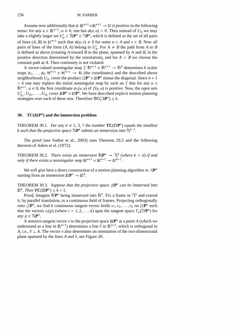
A nonzero tangent vectorv to the projective spaceRPn at a pointA (which weunderstand as a line inRn+1) determines a line ˆv in Rn+1, which is orthogonal toA, i.e., v ⊥ A. The vectorv also determines an orientation of the two-dimensionalplane spanned by the linesA andv, see Figure 20.


Figure20.

For i = 1, 2, . . . , k let Ui ⊂ RPn×RPn denote the open set of all pairs of lines(A, B) in Rn+1 such that the vectorvi(A) is nonzero and the lineB makes an acuteangle with the linevi(A). Let U0 ⊂ RPn × RPn denote the set of pairs of lines(A, B) in Rn+1 making an acute angle.

The setsU0, U1, . . . ,Uk coverRPn ×RPn. Indeed, given a pair (A, B), thereexist indices 1≤ i1 < · · · < in ≤ k such that the vectorsvir (A), wherer = 1, . . . ,n,span the tangent spaceTA(RPn). Then the lines

A, vi1(A), . . . , vin(A)

span the Euclidean spaceRn+1 and therefore the lineB makes an acute angle withone of these lines. Hence, (A, B) belongs to one of the setsU0, Ui1, . . . ,Uik.

We may describe a continuous motion planning strategy over each setUi ,wherei = 0, 1, . . . , k. First define it overU0. Given a pair (A, B) ∈ U0, rotateAtowardB with constant velocity in the two-dimensional plane spanned byA andB so thatA sweeps the acute angle. This defines a continuous motion planningsections0: U0 → P(RPn). The continuous motion planning strategysi : Ui →P(RPn), wherei = 1, 2, . . . , k, is a composition of two motions: first we rotateline A toward the linevi(A) in the in the 2-dimensional plane spanned byA andvi(A) in the direction determined by the orientation of this plane (see above). Onthe second step rotate the linevi(A) towardB along the acute angle similarly tothe action ofs0. ¤

COROLLARY 30.4. One hasTC(RPn) ≤ 2n.Proof. The casen = 1 is trivial. For n > 1 by the Whitney immersion the-

orem there exists an immersionRPn → R2n−1. The result now follows fromTheorem 30.3. ¤

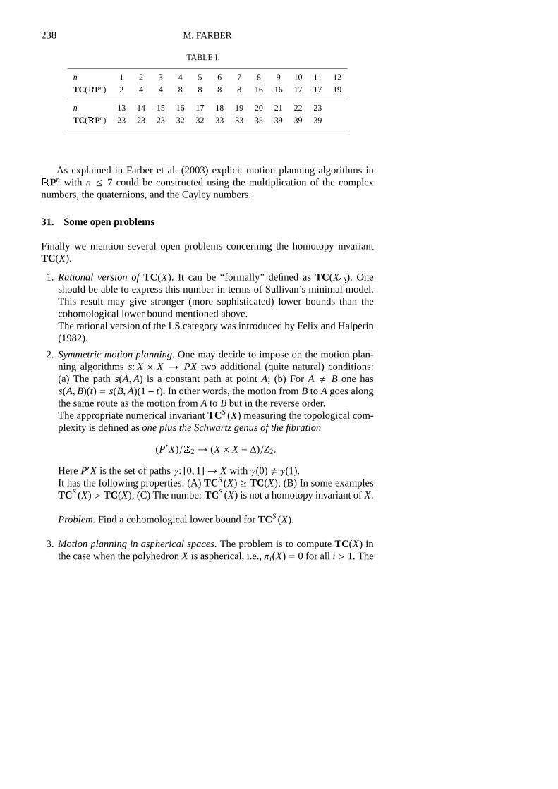
Below is the table of the valuesTC(RPn) for n ≤ 23, see Farber et al. (2003).It is obtained by combining the results mentioned above with the information onthe immersion problem available in the literature.

238 M. FARBER

TABLE I.

n 1 2 3 4 5 6 7 8 9 10 11 12

TC(RPn) 2 4 4 8 8 8 8 16 16 17 17 19

n 13 14 15 16 17 18 19 20 21 22 23

TC(RPn) 23 23 23 32 32 33 33 35 39 39 39

As explained in Farber et al. (2003) explicit motion planning algorithms inRPn with n ≤ 7 could be constructed using the multiplication of the complexnumbers, the quaternions, and the Cayley numbers.

31. Some open problems

Finally we mention several open problems concerning the homotopy invariantTC(X).

1. Rational version ofTC(X). It can be “formally” defined asTC(XQ). Oneshould be able to express this number in terms of Sullivan’s minimal model.This result may give stronger (more sophisticated) lower bounds than thecohomological lower bound mentioned above.The rational version of the LS category was introduced by Felix and Halperin(1982).

2. Symmetric motion planning. One may decide to impose on the motion plan-ning algorithmss: X × X → PX two additional (quite natural) conditions:(a) The paths(A,A) is a constant path at pointA; (b) For A , B one hass(A, B)(t) = s(B,A)(1− t). In other words, the motion fromB to A goes alongthe same route as the motion fromA to B but in the reverse order.The appropriate numerical invariantTCS(X) measuring the topological com-plexity is defined asone plus the Schwartz genus of the fibration

(P′X)/Z2→ (X × X − ∆)/Z2.

HereP′X is the set of pathsγ: [0,1]→ X with γ(0) , γ(1).It has the following properties: (A)TCS(X) ≥ TC(X); (B) In some examplesTCS(X) > TC(X); (C) The numberTCS(X) is not a homotopy invariant ofX.

Problem.Find a cohomological lower bound forTCS(X).

3. Motion planning in aspherical spaces. The problem is to computeTC(X) inthe case when the polyhedronX is aspherical, i.e.,πi(X) = 0 for all i > 1. The


homotopy type of an aspherical spaceX depends only on the fundamentalgroupπ = π1(X). Hence in this case the numberTC(X) depends only on thegroupπ viewed as a discrete group. One should be able to express the numberTC(X) in terms of the algebraic properties of the groupπ1(X).A similar question for the Lusternik – Schnirelmann category was solved byEilenberg and Ganea (1957). Their theorem states:If X is aspherical then

cat(X) − 1 = dimπ = geom dimπ (38)

except3 special low-dimensional cases. Here dimπ is the leastn such thatHq(π; A) = 0 for any moduleA and for anyq > n. The symbol geom dimπdenotes the smallest dimension of aK(π,1)-complex.

References

Abrams, A. (2002) Configuration spaces of colored graphs,Geom. Dedicata92, 185 – 194.Adem, J., Gitler, S., and James, I. M. (1972) On axial maps of a certain type,Bol. Soc. Mat.

Mexicana(2) 17, 59 – 62.Connelly, R., Demaine, E. D., and Rote, G. (2003) Straightening polygonal arcs and convexifying

polygonal cycles,Discrete Comput. Geom.30, 205 – 239.Cornea, O., Lupton, G., Oprea, J., and Tanre, D. (2003)Lusternik – Schnirelmann category, Vol.

103 ofMath. Surveys Monogr., Providence, RI, Amer. Math. Soc.Davis, D. M. (1993) Immersions of projective spaces: a historical survey, In M. C. Tangora (ed.),

Algebraic Topology, Vol. 146 ofContemp. Math., Oaxtepec, 1991, pp. 31–37, Providence, RI,Amer. Math. Soc.

Dold, A. (1972)Lectures on Algebraic Topology, Vol. 200 of Grundlehren Math. Wiss., Berlin,Springer.

Eilenberg, S. and Ganea, T. (1957) On the Lusternik – Schnirelmann category of abstract groups,Ann. of Math.(2) 65, 517 – 518.

Fadell, E. and Neuwirth, L. (1962) Configuration spaces,Math. Scand.10, 111 – 118.Farber, M. (2003) Topological complexity of motion planning,Discrete Comput. Geom.29, 211 –

221.Farber, M. (2004) Instabilities of robot motion,Topology Appl.140, 245 – 266.Farber, M. (2005) Collision free motion planning on graphs, InAlgorithmic Foundations of

Robotics.VI, Utrecht/Zeist, 2004, Berlin, Springer, to appear.Farber, M., Tabachnikov, S., and Yuzvinsky, S. (2003) Topological robotics: motion planning in

projective spaces,Int. Math. Res. Not.34, 1853 – 1870.Farber, M. and Yuzvinsky, S. (2004) Topological robotics: subspace arrangements and collision

free motion planning, In V. M. Buchstaber and I. M. Krichever (eds.),Geometry, Topology, andMathematical Physics, Vol. 212 ofAmer. Math. Soc. Transl. Ser.2, Moscow, 2002 – 2003, pp.145–156, Providence, RI, Amer. Math. Soc.

Felix, Y. and Halperin, S. (1982) Rational LS category and its applications,Trans. Amer. Math. Soc.273, 1 – 38.

Gal, S. (2001) Euler characteristic of the configuration space of a complex,Colloq. Math.89,61 – 67.

Ghrist, R. (2001) Configuration spaces and braid groups on graphs in robotics, In J. Gilman, W. W.Menasco, and X.-S. Lin (eds.),Knots, Braids, and Mapping Class Groups — Papers Dedicated

240 M. FARBER

to Joan S. Birman, Vol. 24 ofAMS/IP Stud. Adv. Math., New York, 1998, pp. 29–40, Providence,RI, Amer. Math. Soc. & Somerville, MA, International Press.

Ghrist, R. W. and Koditschek, D. E. (2002) Safe cooperative robot dynamics on graphs,SIAM J.Control Optim.40, 1556 – 1575.

Hausmann, J.-C. and Knutson, A. (1998) Cohomology rings of polygon spaces,Ann. Inst. Fourier(Grenoble) 48, 281 – 321.

Jordan, D. and Steiner, M. (1999) Configuration spaces of mechamical linkages,Discrete Comput.Geom.22, 297 – 315.

Kapovich, M. and Millson, J. J. (1996) The symplectic geometry of polygons in Euclidean space,J. Differential Geom.44, 479 – 513.

Kapovich, M. and Millson, J. J. (2002) Universality theorems for configuration spaces of planarlinkages,Topology41, 1051 – 1107.

Klyachko, A. A. (1994) Spatial polygons and stable configurations of points in the projective line,In Algebraic Geometry and its Applications, Vol. E25 of Aspects Math., Yaroslavl′, 1992, pp.67–84, Braunschweig, Vieweg.

Lam, K. Y. (1967) Construction of nonsingular bilinear maps,Topology6, 423 – 426.Latombe, J.-C. (1991)Robot Motion Planning, Dordrecht, Kluwer Acad. Publ.Lebesgue, H. (1950)Lecons sur les constructions geometriques, Paris, Gauthier-Villars.Milgram, R. J. (1967) Immersing projective spaces,Ann. of Math.(2) 85, 473 – 482.Orlik, P. and Terao, H. (1992)Arrangements of Hyperplanes, Vol. 300 ofGrundlehren Math. Wiss.,

Berlin, Springer.Schwartz, J. T. and Sharir, M. (1983) On the “piano movers” problem. II. General techniques for

computing topological properties of real algebraic manifolds,Adv. in Appl. Math.4, 298 – 351.Schwarz, A. S. (1966) The genus of a fiber space,Amer. Math. Soc. Transl.(2) 55, 49–140.Sharir, M. (1997) Algorithmic motion planning, In J. E. Goodman and J. O’Rourke (eds.),Hand-

book of Discrete and Computational Geometry, CRC Press Ser. Discrete Math. Appl., BocaRaton, FL, CRC Press, p. 733 – 754.

Smale, S. (1987) On the topology of algorithms. I,J. Complexity3, 81 – 89.Swia↪tkowski, J. (2001) Estimates for the homological dimension of configuration spaces of graphs,

Colloq. Math.89, 69 – 79.Thurston, W. (1987) Shapes of polyhedra, preprint.Vassil′iev, V. A. (1988) Cohomology of braid groups and complexity of algorithms,Funktsional.

Anal. i Prilozhen.22, 15 – 24, (Russian); English transl. in Funct. Anal. Appl.22, 182 – 190.Walker, K. (1985) Configuration spaces of linkages, Undergraduate thesis, Princeton University.

Documents

TOPOLOGY OF ROBOT MOTION PLANNING Michael …shmuel/AAT-readings/Robotics...TOPOLOGY OF ROBOT MOTION PLANNING Michael Farber University of Durham Abstract. In this paper we discuss