Topology, geometry and quantum interference in

condensed matter physics

Alexander G. Abanov

Department of Physics and Astronomy andSimons Center for Geometry and Physics,

Stony Brook University,Stony Brook, NY 11794, USA

August 25, 2017

Abstract

The methods of quantum field theory are widely used in condensed matter physics. In par-ticular, the concept of an effective action was proven useful when studying low temperature andlong distance behavior of condensed matter systems. Often the degrees of freedom which ap-pear due to spontaneous symmetry breaking or an emergent gauge symmetry, have non-trivialtopology. In those cases, the terms in the effective action describing low energy degrees offreedom can be metric independent (topological). We consider a few examples of topologicalterms of different types and discuss some of their consequences. We will also discuss the originof these terms and calculate effective actions for several fermionic models. In this approach,topological terms appear as phases of fermionic determinants and represent quantum anomaliesof fermionic models. In addition to the wide use of topological terms in high energy physics,they appeared to be useful in studies of charge and spin density waves, Quantum Hall Effect,spin chains, frustrated magnets, topological insulators and superconductors, and some modelsof high-temperature superconductivity.

These notes are based on the lectures given by the author at “SERC School on Topology andCondensed Matter Physics” in Kolkata, India in December 2015.

Contents

1 Introductory remarks 11.1 Theory of Everything in condensed matter physics . . . . . . . . . . . . . . . . . . . 11.2 Spontaneous symmetry breaking and an emergent topology . . . . . . . . . . . . . . 21.3 Additional reading . . . . . . . . . . . . . . . . . . . . . . . . . . . . . . . . . . . . . 4

2 Motivating example: a particle on a ring. 42.1 Classical particle on a ring: Action, Lagrangian, and Hamiltonian . . . . . . . . . . . 42.2 Quantum particle on a ring: Hamiltonian and spectrum . . . . . . . . . . . . . . . . 52.3 Quantum particle on a ring: path integral and Wick’s rotation . . . . . . . . . . . . 72.4 Quantum doublet . . . . . . . . . . . . . . . . . . . . . . . . . . . . . . . . . . . . . . 82.5 Full derivative term and topology . . . . . . . . . . . . . . . . . . . . . . . . . . . . . 82.6 Topological terms and quantum interference . . . . . . . . . . . . . . . . . . . . . . . 9

i

arX

iv:1

708.

0719

2v1

[co

nd-m

at.s

tr-e

l] 2

3 A

ug 2

017

2.7 General definition of topological terms . . . . . . . . . . . . . . . . . . . . . . . . . . 92.8 Theta terms and their effects on the quantum problem . . . . . . . . . . . . . . . . . 92.9 Exercises . . . . . . . . . . . . . . . . . . . . . . . . . . . . . . . . . . . . . . . . . . 10

3 Path integral for a single spin. 113.1 Quantum spin . . . . . . . . . . . . . . . . . . . . . . . . . . . . . . . . . . . . . . . . 113.2 Fermionic model . . . . . . . . . . . . . . . . . . . . . . . . . . . . . . . . . . . . . . 14

Effective action by chiral rotation trick . . . . . . . . . . . . . . . . . . . . . . . . . . 14Topological term . . . . . . . . . . . . . . . . . . . . . . . . . . . . . . . . . . . . . . 17Path integral representation of quantum spin . . . . . . . . . . . . . . . . . . . . . . 17

3.3 Derivation of a WZ term from fermionic model without chiral rotation . . . . . . . . 183.4 Quantum spin as a particle moving in the field of Dirac monopole . . . . . . . . . . . 193.5 Reduction of a WZ term to a theta-term . . . . . . . . . . . . . . . . . . . . . . . . . 193.6 Properties of WZ terms . . . . . . . . . . . . . . . . . . . . . . . . . . . . . . . . . . 193.7 Exercises . . . . . . . . . . . . . . . . . . . . . . . . . . . . . . . . . . . . . . . . . . 20

4 Spin chains. 234.1 Path integral for quantum magnets . . . . . . . . . . . . . . . . . . . . . . . . . . . . 23

Path integral for the magnet on a lattice . . . . . . . . . . . . . . . . . . . . . . . . . 23Continuum limit for Quantum Ferromagnet . . . . . . . . . . . . . . . . . . . . . . . 24Bloch’s law: the dispersion of spin waves in ferromagnet . . . . . . . . . . . . . . . . 25

4.2 Continuum path integral for Quantum Antiferromagnet . . . . . . . . . . . . . . . . 254.3 RG for O(3) NLSM . . . . . . . . . . . . . . . . . . . . . . . . . . . . . . . . . . . . . 274.4 O(3) NLSM with topological term . . . . . . . . . . . . . . . . . . . . . . . . . . . . 284.5 Boundary states for spin 1 chains with Haldane’s gap . . . . . . . . . . . . . . . . . . 314.6 AKLT model . . . . . . . . . . . . . . . . . . . . . . . . . . . . . . . . . . . . . . . . 314.7 Exercises . . . . . . . . . . . . . . . . . . . . . . . . . . . . . . . . . . . . . . . . . . 33

5 Conclusion 34

6 Acknowledgements 35

A Appendix: Topological defects and textures 38

B Appendix: Integrating out l field 39

C Appendix: Homotopy groups often used in physics 40

1 Introductory remarks

1.1 Theory of Everything in condensed matter physics

In condensed matter physics, we believe that we know the “Theory of Everything” – the fundamen-tal equations potentially describing all observable phenomena in condensed matter physics. Essen-tially, those equations are Schrodinger equations for electrons and nuclei, together with Maxwellequations describing electromagnetic interactions. [1] However, there is a long way from knowingfundamental equations and being able to actually describe collective behavior of 1020 or so nucleiand electrons forming condensed matter systems, like, liquids, solids, superfluids, superconductors,

1

quantum Hall systems etc. Having “more” particles makes macroscopic systems behave very differ-ently from collections of just a few particles. New qualitative features appear when one goes frommicroscopic to macroscopic systems. [2] We refer to new phenomena appearing at macroscopicscales as to “emergent phenomena”.

The goal of condensed matter physics is not finding fundamental laws but rather finding theirconsequences. In particular, we are interested in finding efficient ways to describe emergent macro-scopic phenomena. While it is very hard to derive macroscopic phenomena by solving fundamentalequations we have a few guiding principles that allow us to write effective descriptions of thosephenomena. Such principles include the use of symmetries and associated conservation laws, mech-anisms of spontaneous symmetry breaking, the concept of quasiparticles etc. Early examples ofeffective descriptions include thermodynamics and hydrodynamics.

In these lectures, we focus on the “topological properties” of condensed matter systems andtheir descriptions. Topological properties, in general, are the properties robust with respect tocontinuous deformations. They are emergent properties and it is important to understand themin the context of condensed matter physics as they might be the most stable properties insensitiveto deformations and perturbations always present in realistic materials. The main focus of theselectures will be on topological properties related to quantum physics.

1.2 Spontaneous symmetry breaking and an emergent topology

If there were no separation of scales in Nature, the task of theoretical physicists would be formidable.Fortunately, in many cases one can “integrate out” fast degrees of freedom and effectively describeproperties of microscopic systems at low temperatures, low frequencies, and large distances usingrelatively simple continuous field theory descriptions. This happens due to the presence of exactor approximate symmetries in the underlying microscopic system. More precisely, it is due to aphenomenon of spontaneous symmetry breaking.

Suppose that the exact Hamiltonian of some condensed matter system has some continuoussymmetry given by Lie group G. A good system to keep in mind as an example is an isotropicferro- or antiferromagnet with an SU(2) symmetry with respect to global rotations of all spins.Then it is possible that at some values of parameters of the Hamiltonian,1 the ground state ofthe system breaks the symmetry up to some subgroup H of G. If this happens, we say that thesymmetry of the Hamiltonian is spontaneously broken by its ground state. One can characterizethis ground state by some element n of a coset space G/H. In our example of the magnet we takeH = SO(2) = U(1) and G/H = SU(2)/U(1) = S2. The element of a coset space in this caseis a point of two-dimensional sphere S2 which labels the direction of magnetization of our systemand subgroup H is just the group of all rotations around the direction of magnetization which isobviously a symmetry of the Hamiltonian and of the ground state of the system. In the presenceof spontaneous breaking of a continuous symmetry the ground state is infinitely degenerate, sinceany n ∈ G/H gives the ground state with the same energy. Indeed, any two states characterizedby n1, n2 ∈ G/H have the same energy since they can be transformed into one another by someelement g ∈ G, which is an exact symmetry transformation of the Hamiltonian.

Now consider another state of the quantum system which locally, in the vicinity of spatialpoint x, is very close to the ground state of the system labeled by some n(x) ∈ G/H. We assumethat n(x) is not constant in space but changes very slowly with a typical wavenumber k. Insuch a case, n(x) is called an order parameter of the system. We denote the energy of this stateper unit volume measured from the energy of the ground state ε(k). The limit of small k → 0

1We consider here the case of zero temperature for simplicity.

2

corresponds to the order parameter which is constant in space n(x) = n0 and, therefore, ε(k)→ 0as k → 0. We obtain that when continuous symmetry is spontaneously broken, the ground stateof the system is not isolated but there are always excited states whose energies are infinitesimallyclose to the ground state energy. These heuristic arguments can be made more rigorous and leadto the Goldstone theorem2. The theorem states that in quantum field theory with spontaneouslybroken continuous symmetry there are massless particles which energy ε(k)→ 0 as k → 0.

If one is interested in low energy physics one necessarily should take these massless modes(or Goldstone bosons) into account. Moreover, the nature of these massless modes is dictatedessentially by the symmetry (and its breaking) of the system, and one expects, therefore, that thecorrect low energy description should depend only on symmetries of the system but not on its everymicroscopic detail.

A natural variable describing the dynamics of Goldstone modes is the order parameter itself. Forexample, in the case of relativistically invariant system described by the order parameter n ∈ S2,we immediately write

SNLSM =

∫dd+1x

1

2g(∂µn)2 + (other terms). (1)

We have written here the most obvious term of an effective action which is both Lorentz invariantand SU(2) invariant (with respect to rotations of a unit, three-component vector n2 = 1). Here gis a coupling constant which should be obtained from a detailed microscopic theory. The “otherterms” are the terms which are higher order in gradients and (possibly) topological terms. Themodel (1) is referred to as a “non-linear σ-model”3. In different spatial dimensions, higher gradientterms of non-linear σ-models might be relevant. We are not discussing those terms as well asthe issue of renormalizability of σ-models, concentrating instead on the allowed topological terms.Therefore, we will keep only the kinetic term 1

2g (∂µn)2 in the gradient expansion of an effectiveLagrangian as well as all allowed topological terms.

Before proceeding to our main subject – topological terms, let us make two important remarks.Firstly, very often (especially in condensed matter systems) the symmetries of the Hamiltonianare approximate and there are terms in the Hamiltonian which explicitly but weakly break thesymmetry. This does not invalidate the speculations of this section. The difference will be thatwould-be-Goldstone particles acquire small mass. The weaker the explicit symmetry breaking of theHamiltonian the smaller is the mass of “Goldstone” particles. One can proceed with the derivationof the non-linear σ-model which will contain weak symmetry breaking terms (such as easy-axisanisotropy for magnets). This model will have non-trivial dynamics at energies bigger than thesmallest of masses.

Second remark is that there are other mechanisms in addition to the spontaneous symmetrybreaking which result in low energy excitations. One of the most important mechanisms is realizedwhen local (or gauge) symmetry is present. Then, gauge invariance plus locality demands thepresence of massless particles (e.g, photons) in the system. The low energy theories in this caseare gauge theories. Similar to an explicit symmetry breaking in case of Goldstone particles thereare mechanisms which generate masses for gauge bosons. These are, e.g., Higgs mechanism and

2For a full formulation of the Goldstone theorem for relativistic field theory as well as for its proof see e.g., [3].We avoid it here because we are generally interested in a wider range of systems, e.g., without Lorentz invariance.There are still some analogs of the Goldstone theorem there. For example in the case of a ferromagnet there are stillmassless particles – magnons. However, the number of independent massless particles is not correctly given by theGoldstone theorem for relativistic systems.

3The origin of the term is in effective theories of weak interactions [4, 5]. Non-linear comes from the non-linearrealization of symmetries in this model. E.g., constraint n2 = 1 is non-linear. Sigma (σ) is a historic notation for the“order parameter” in theories of weak interactions.

3

confinement of gauge fields. We will have some examples of topological terms made out of gaugefields in these lectures although our main focus will be on non-linear sigma models4. We also donot consider here cases with massless fermionic degrees of freedom we concentrate exclusively onbosonic effective theories.

1.3 Additional reading

The focus of these lectures is on the effect of topological terms in the action on physical propertiesof condensed matter systems. We are not discussing here classification of topological defects intextures in ordered media. The latter is a well developed subject (see the classical review [7]). Forreader’s convenience we collected a few exercises on topological textures and related examples inAppendix A.

The subject of topological terms or broader “topological phases of matter” is huge, and we donot do it justice in these lectures. In particular, I do not try to give a complete bibliography inthese lectures. Instead, with a few exceptions I refer not to the original papers but to textbooks orreviews.

Homotopy classification of topological defects and textures in ordered media is not discussed inthis lectures. However, it is a necessary prerequisite to understanding topological terms discussedhere. I recommend a classic reference [7]. To make this text more self-contained I also collectedfew exercises on that topic in Appendix A and relevant homotopy groups in Appendix C.

I would recommend the following textbooks close in spirit to the point of view presented here[6, 8, 9]. Some of the technical details of fermionic determinant calculations can be found in [10, 11].Topological terms are intimately related to geometric or Berry phases [12] and to quantum anomaliesin field theories [13].

In these lectures, I avoid using any advanced topological and geometrical tools. However, Ihighly recommend studying all necessary mathematics seriously. There are many beautiful booksthat give good introduction to the subject for physicists. See, for example Refs. [14, 15, 16, 17, 18].

2 Motivating example: a particle on a ring.

2.1 Classical particle on a ring: Action, Lagrangian, and Hamiltonian

As a simple motivating example let us consider a particle on a ring. Classically, the motion can bedescribed by the principle of least action. A classical action S of a particle can be taken as

S[φ] =

∫dtL(φ, φ), (2)

L =M

2φ2 +Aφ, (3)

should be minimal (locally) on classical trajectories. Here, the angle φ(t) is chosen to be a general-ized coordinate of the particle on a ring, M is a moment of inertia of a particle (or mass for a unitring), A is some constant.

Euler-Langrange equations of motion are given in terms of Lagrangian L by ddt∂L∂φ− ∂L

∂φ = 0, or

explicitlyMφ = 0. (4)

4Non-linear sigma models and gauge theories have a lot in common [6].

4

A particle, given an initial velocity, moves with constant angular velocity along the ring. Notice,that the last term of (3) does not have any effect on the motion of the particle. Indeed, this termis a total time derivative and can not affect the principle of least action [19].

Given an initial position of a particle on a ring at t = t1 and a final position at t = t2 thereare infinitely many solutions of (4). They can be labeled by the integer number of times particlegoes around the ring to reach its final position. This happens because of nontrivial topology of thering – one should identify φ = φ + 2π as labeling the same point on the ring. This is not veryimportant classically as we can safely think of the angle φ taking all real values from −∞ to +∞.Given initial position φ(t1) = φ1 and initial velocity φ(t1) = ω1 one can unambiguously determinethe position of the particle φ(t) at all future times using (4).

Let us now introduce the momentum conjugated to φ as

p =∂L

∂φ= Mφ+A, (5)

and the Hamiltonian as

H = pφ− L =1

2M(p−A)2. (6)

Corresponding Hamilton equations of motion

φ =1

M(p−A), (7)

p = 0, (8)

are equivalent to (4).Notice that although the parameter A explicitly enters Hamiltonian formalism, it only changes

the definition of generalized momentum Mφ + A instead of more conventional Mφ. It does notchange the solution of equations of motion and can be removed by a simple canonical transformationp→ p+A. We will see below that this changes for a quantum particle.

2.2 Quantum particle on a ring: Hamiltonian and spectrum

Let us now consider a quantum particle on a ring. We replace classical Poisson’s bracket p, φ = 1by quantum commutator [p, φ] = −ih and use φ-representation, i.e., we describe our states by wavefunctions on a ring ψ(φ). In the following, we will put h = 1. In this representation, we can usep = −i∂φ and rewrite (6) as a quantum Hamiltonian

H =1

2M(−i∂φ −A)2 . (9)

The eigenstates and eigenvalues of this Hamiltonian are given by solutions of stationary Schrodingerequation Hψ = Eψ. We impose periodic boundary conditions requiring ψ(φ + 2π) = ψ(φ), i.e.,the wave function is required to be a single-valued function on the ring. The eigenfunctions andeigenvalues of (9) are given by

ψm = eimφ, (10)

Em =1

2M(m−A)2, (11)

where m = 0,±1,±2, . . . is any integer number - the quantized eigenvalue of the momentum

operator p = −i∂φ. We notice that although the classical model is not sensitive to the parameter

5

Figure 1: The spectrum of the particle on a ring is shown for A = θ/2π = 0, 1/2, 1/4 respectively.The classical energy E(p) is represented by a parabola and does not depend on the parameter A.

A, the quantum one is, because of the quantization of p. The parameter A can be interpreted as avector potential of the magnetic flux penetrating the ring. This vector potential is not observablein classical mechanics but affects the quantum spectrum because of multiple-connectedness of thering (there are many non-equivalent ways to propagate from the point 1 to the point 2 on a ring).More precisely our parameter A should be identified with the vector potential multiplied by e

hc . It

corresponds to the magnetic flux through the ring Φ = AΦ0, where Φ0 is a flux quantum Φ0 = 2π hce .The A-term of the classical action – topological term – can be written as

Stop =

∫ t2

t1

dtAφ = 2πAφ2 − φ1

2π= θ

∆φ

2π. (12)

It depends only on the initial and final values φ1,2 = φ(t1,2) and changes by θ = 2πA every time theparticle goes a full circle around the ring in counterclockwise direction. The conventional notation θfor a coefficient in front of this term gave the name topological theta-term for this type of topologicalterms.

The spectrum (11) is shown in Figure 1 for three values of flux through the ring: θ = 0, π, π/2(A = Φ/Φ0 = 0, 1, 1/2).

Several comments are in order. (i) An integer flux A-integer or θ - multiple of 2π does notaffect the spectrum. (ii) There is an additional symmetry (parity) of the spectrum when θ is amultiple of π (integer or half-integer flux). (iii) For half-integer flux θ = π, the ground state isdoubly degenerate E0 = E1.

Finally, let us try to remove the A term by canonical transformation as in the classical case.We make a gauge transformation ψ → eiAφψ and obtain p → p + A and H = 1

2M (−i∂φ)2. Onemight think that we removed the effects of the A term completely. However, this transformationchanges the boundary conditions of the problem replacing them by twisted boundary conditionsψ(φ + 2π) = e−i2πAψ(φ). The eigenfunctions satisfying twisted boundary conditions are ψm =ei(m−A)φ and produce the same eigenvalues (11). We conclude that it is not possible to remove theeffects of topological A-term in quantum mechanics. The parameter A can be formally removedfrom the Hamiltonian by absorbing it into the boundary conditions. This, however, does not changethe spectrum and other physical properties of the system.

6

2.3 Quantum particle on a ring: path integral and Wick’s rotation

Quantum mechanics of a particle on a ring described by the classical action (3) can be representedby path integral

Z =

∫Dφ eiS[φ], (13)

where integration is taken over all possible trajectories φ(t) (with proper boundary values). In thisapproach the contribution of the topological term to the weight in the path integral is the phaseeiθ∆φ/(2π) which is picked up by a particle moving in the presence of the vector potential.

Let us perform Wick’s rotation replacing the time by an imaginary time τ = it. Then∫dtMφ2

2→ i

∫dτ

Mφ2

2, (14)∫

dtAφ →∫dτ Aφ, (15)

where in the r.h.s dot means the derivative with respect to τ . The path integral (13) is then replacedby a Euclidean path integral

Z =

∫ei[φ(T )−φ(0)]=1

Dφ e−S[φ], (16)

where the action

S =

∫ β

0dτ

[M

2φ2 − iAφ

]. (17)

We considered the amplitude of the return to the initial point in time β, i.e. 0 < τ < β. Thisrequires periodic boundary conditions in time eiφ(0) = eiφ(β).

We notice here that because the A-term is linear in time derivative it does not change its formunder Wick’s rotation (15) and therefore, is still imaginary in Euclidean formulation (17). Withoutimaginary term one could think about e−S as of the Boltzmann weight in the classical partitionfunction.

One can satisfy the boundary conditions as φ(β) − φ(0) = 2πQ with any integer Q. We canrewrite the partition function (16) as:

Z =+∞∑

Q=−∞eiθQ

∫φ(β)−φ(0)=2πQ

Dφ e−∫ β0 dτ M

2φ2. (18)

We notice here that θ = 2πn – multiple of 2π – is equivalent to θ = 0. Second, we noticethat the partition function is split into the sum of path integrals over distinct topological sectorscharacterized by an integer number Q which is called the winding number. The contributions oftopological sectors to the total partition function are weighed with the complex weights eiθQ.

For future comparisons, let us write (17) in terms of a unit two-component vector ∆ =(∆1,∆2) = (cosφ, sinφ), ∆2 = 1.

S =

∫ β

0dτ

[M

2∆2 − iA(∆1∆2 −∆2∆1)

]. (19)

This is the simplest (0 + 1)-dimensional O(2) non-linear σ-model.

7

2.4 Quantum doublet

Let us consider a particular limit of a very light particle on a circle M → 0 in the presence of halfof the flux quantum A = 1/2, θ = π. With this flux, the ground state of the system is doublydegenerate E0 = E1 and the rest of the spectrum is separated by the energies ∼ 1/M → ∞ fromthe ground state (11). At large β (low temperatures) we can neglect contributions of all statesexcept for the ground state.

We write the general form of the ground state wave function as α| + 1/2〉 + β| − 1/2〉, where|+1/2〉 = ψ0 and |−1/2〉 = ψ1. The ground state space (α, β) coincides with the one for a spin 1/2.One might say that (16-17) with M → 0 realize a path integral representation for the quantumspin 1/2. This representation does not have an explicit SU(2) symmetry. We will consider anSU(2)-symmetric path integral representation for quantum spins later.

Meanwhile, let us discuss some topological aspects of a plane rotator problem.

2.5 Full derivative term and topology

From a mathematical point of view, the motion of a particle on a unit circle with periodic boundaryconditions in time is described by a mapping φ(τ) : S1

τ → S1φ of a circle formed by compactified

time S1τ = τ ∈ [0, β] into a circle S1

φ = φ ∈ [0, 2π]. This mapping can be characterized by integer

winding number Q which tells us how many times the image φ goes around target space S1φ when

variable τ changes from 0 to β.It can be shown that two such mappings φ1(τ) and φ2(τ) can be continuously deformed into one

another if and only if they have the same winding number. Therefore, all mappings are divided intotopological classes enumerated by Q = 0,±1,±2, . . .. Moreover, one can define a group structureon topological classes. First, we define the product of two mappings φ1 and φ2 as

φ2 · φ1(τ) =

φ1(2τ), for 0 < τ < β/2 ,φ1(β) + φ2(2τ − β), for β/2 < τ < β .

If φ1 belongs to the topological class Q1 and φ2 to Q2, their product belongs to the class Q1 +Q2.One can say that the product operation on mappings induces the structure of Abelian group onthe set of topological classes. In this case this group is the group of integer numbers with respectto addition. One can write this fact down symbolically as π1(S1) = Z, where subscript one denotesthat our time is S1 and S1 in the argument is our target space. One says that the first (orfundamental) homotopy group of S1 is the group of integers.

There is a simple formula giving the topological class Q ∈ Z in terms of φ(τ)

Q =

∫ β

0

dτ

2πφ . (20)

Let us now assume that we split our partition function into the sum over different topologicalclasses. What are the general restrictions on the possible complex weights which one can introducein the physical problem. One can deform smoothly any mapping in the class Q1 + Q2 into twomappings of classes Q1 and Q2 which are separated by a long time. Because of the multiplicativeproperty of amplitudes, this means that the weights WQ associated with topological classes mustform a (unitary) representation of the fundamental group of a target space. The only unitaryrepresentation of Z is given by WQ = eiθQ with 0 < θ < 2π labelling different representations. Inthe case of plane rotator, these weights correspond to a phase due to the magnetic flux piercingthe one-dimensional ring.

8

In more general case of, say, particle moving on the manifold G (instead of S1) we have toconsider the fundamental group of the target space π1(G), find its unitary representations, andobtain complex weights which could be associated with different topological classes.

2.6 Topological terms and quantum interference

As it can be seen from (18) the presence of a topological term in the action (θ 6= 0) results in theinterference between topological sectors in the partition function. The Boltzmann weight calculatedfor a trajectory within a given topological sector Q is additionally weighted with complex phaseeiθQ. This interference can not be removed by Wick’s rotation.

2.7 General definition of topological terms

We define generally topological terms as metric-independent terms in the action.A universal object present in any local field theory is the symmetric stress-energy tensor Tµν .

It can be defined as a variation of the action with respect to the metric gµν . More precisely, aninfinitesimal variation of the action can be written as

δS =

∫dx√g Tµνδg

µν , (21)

where√g dx is an invariant volume of space-time.

It immediately follows from our definition of topological terms that they do not contribute tothe stress-energy tensor. If in a field theory all terms are topological we have Tµν = 0 for such atheory. These theories are called topological field theories.

A particular general covariant transformation is the rescaling of time. Topological terms do notdepend on a time scale. Therefore, the corresponding Lagrangians are linear in time derivatives.They do not transform under Wick’s rotation and are always imaginary in Euclidean formulation.They describe quantum interference which is not removable by Wick rotation.

2.8 Theta terms and their effects on the quantum problem

Theta terms are topological terms of a particular type. They appear when there exist nontrivialtopological textures in space-time. Essentially, these terms are just complex weights of differenttopological sectors in the path integration. We will go over more details on θ-terms later in thecourse.

In addition to being imaginary in Euclidean formulation as all other topological terms, θ-terms have also some special properties. These properties distinguish them from other types oftopological terms. The following is a partial list of the features of topological θ-terms and of theirmanifestations.

• θ-terms assign complex weights in path integral to space-time textures with integer topologicalcharge Q

• Realize irreducible 1d-representations of πD(G), where D is the dimension of space-time andG is a target space

• Quantum interference between topological sectors

• Do not affect equations of motion

• Affect the spectrum of a quantum problem by changing quantization rules

9

• Periodicity in coupling constant θ 5.

• θ is not quantized (for Q ∈ Z)

• For θ = 0, π, there is an additional (parity) symmetry

• θ = π – degeneracy of the spectrum. Gapless excitations.

• Equivalent to changes in boundary conditions.

• θ is a new parameter which appears from the ambiguity of quantization of the classicalproblem for multiply-connected configurational space.

2.9 Exercises

Exercise 1: Particle on a ring, path integral

The Euclidean path integral for a particle on a ring with magnetic flux through the ring is given by

Z =

∫Dφ e−

∫ β0dτ(mφ2

2 −iθ2π φ

).

Using the decomposition

φ(τ) =2π

βQτ +

∑l∈Z

φlei 2πβ lτ ,

rewrite the partition function as a sum over topological sectors labeled by winding number Q ∈ Z andcalculate it explicitly. Find the energy spectrum from the obtained expression.

Hint : Use summation formula+∞∑

n=−∞e−

12An

2+iBn =

√2π

A

+∞∑l=−∞

e−1

2A (B−2πl)2 .

Exercise 2: Spin 1/2 from a particle on a ring

Calculate the partition function of a particle on a ring described in the previous exercise. Find explicitexpressions in the limit m→ 0, θ → π but θ − π ∼ m/β. One can interpret the obtained partition functionas a partition function of a spin 1/2. What is the physical meaning of the ratio (θ − π)/m in the spin 1/2interpretation of the result?

Hint : see Sec. 2.4.

Exercise 3: Metric independence of the topological term

The classical action of a particle on a ring is given by

S =

∫dtp

(mφ2

2− θ

2πφ

),

where tp is some “proper” time. Reparametrizing time as tp = f(t) we have dtp = f ′dt and dt2p = f ′2dt2

and identify the metric as g00 = f ′2

and g00 = f ′−2

. We also have√g00 = f ′. Rewrite the action in terms

of φ(t) instead of φ(tp). Check that it has a proper form if written in terms of the introduced metric. Usingthe general formula for variation of the action with respect to a metric (g = det gµν)

δS =1

2

∫dx√g Tµνδg

µν ,

find the stress-energy tensor for a particle on a ring. Check that T00 is, indeed, the energy of the particle.

5We assume that configurations are smooth and the space-time manifold is closed (no boundary)

10

3 Path integral for a single spin.

Wess and Zumino introduced an effective Lagrangian to summarize the anomalies in current alge-bras [20]. E. Witten considered global (topological) aspects of this effective action [21]. Simulta-neously, S. P. Novikov studied multi-valued functionals [22]. The corresponding topological termsare referred to as Wess-Zumino-Novikov-Witten terms or more often as just Wess-Zumino terms.In this section, we consider the simplest quantum mechanical (0+1 dimensional) version of such aterm which is relevant for path integral formulation of a quantum mechanics of a single spin.

3.1 Quantum spin

Let us consider a simple example of how Wess-Zumino effective Lagrangian appears from the“current algebra”. To simplify the story we take an example of quantum spin S. This is a quantummechanical system with an SU(2) spin algebra playing the role of “current algebra” of quantumfield theory. We have standard spin commutation relations

[Sa, Sb] = iεabcSc, (22)

where a, b, c take values x, y, z. We require that

S2 = S(S + 1), (23)

where 2S is an integer number defining the representation (the value of spin). Let us consider thesimplest possible Hamiltonian of a quantum spin in a constant magnetic field

H = −h · S (24)

and derive an operator equation of motion

∂tS = i[H,S] = −i[h · S,S] = S× h. (25)

In the classical limit S → ∞ (or h → 0) it is convenient to write S → Sn so that n is a classicalunit vector n2 = 1 and equation of motion(25) becomes classical equation of motion

∂tn = n× h. (26)

The natural question immediately occurs is what classical action corresponds to this equation ofmotion. It turns out that writing down this action is not completely trivial problem if one desiresfor the action to have explicitly SU(2) invariant form. Let us first derive it using non-invariantparameterization in terms of spherical angles n = (sin θ cosφ, sin θ sinφ, cos θ). We assume that theangle θ is measured from the direction of magnetic field h = (0, 0, h). The Hamiltonian (24) becomesH = −hS cos θ and equations of motion (26) become φ = −h and θ = 0 – precession around thedirection of magnetic field. We obtain these equations as Hamilton’s equations, identifying themomentum conjugated to φ coordinate as

pφ = −S(1− cos θ). (27)

Then the classical action of a single spin in magnetic field can be written as

S[n] = −4πSW0 +

∫dt Sh · n, (28)

11

Figure 2: The unit vector n(τ) draws a closed line on the surface of a sphere with unit radiusduring its motion in imaginary time. Berry phase is proportional to the solid angle (shaded region)swept by the vector n(t). One can calculate this solid angle by extending n into the two-dimensionaldomain B as n(ρ, t) and calculating (30).

where W0 is defined using a particular choice of coordinates as

W0 =1

4π

∫dt (1− cos θ)∂tφ =

1

4π

∫dφ (1− cos θ) =

Ω

4π, (29)

where Ω is a solid angle encompassed by the trajectory of n(t) during time evolution. The firstterm in the action (28) has a form of

∫dt pφφ and the second is a negative time integral of the

Hamiltonian.Although (29) has a nice geometrical meaning it is written in some particular coordinate system

on two-dimensional sphere. It would be nice to have an expression for W0 which is coordinateindependent and explicitly SU(2) invariant (with respect to rotations of n). Such a form, indeedexists

W0 =

∫ 1

0dρ

∫ β

0dt

1

8πεµνn · [∂µn× ∂νn] . (30)

Here we assume periodic boundary conditions in time n(β) = n(0), ρ is an auxiliary coordinateρ ∈ [0, 1]. n-field is extended to n(t, ρ) in such a way that n(t, 0) = (0, 0, 1) and n(t, 1) = n(t).Indices µ, ν take values t, ρ.

Wess-Zumino action (30) has a very special property. Although it is defined as an integral overtwo-dimensional disk parameterized by ρ and t its variation depends only on the values of n on theboundary of the disk—physical time. Indeed one can check that

δW0 =

∫ 1

0dρ

∫ β

0dt

1

4πεµνn · [∂µδn× ∂νn]

=

∫ 1

0dρ

∫ β

0dt ∂µ

1

4πεµνn · [δn× ∂νn]

=

1

4π

∫ β

0dt δn [n× n] , (31)

where we used that δn · [∂µδn× ∂νn] = 0 because all three vectors δn, ∂µn, and ∂νn lie in the sameplane (tangent to the two-dimensional sphere n2 = 1. Due to this property classical equation ofmotion does not depend on the arbitrary extension of n to ρ 6= 1.

12

B

B

t

+

-

n

Figure 3: Two extensions n(t, ρ) and n′(t, ρ) define a mapping S2 → S2. The difference W0[n]−W0[n′] gives a winding number of this mapping.

In quantum physics, however, not only the variation δW0 but the weight e2πiW0 should notdepend on unphysical configuration n(t, ρ) but only on n(t, ρ = 1). To see that this is indeed so,we consider the configuration n(t, ρ) as a mapping from two-dimensional disk (t, ρ) ∈ B+ into thetwo-dimensional sphere n ∈ S2. Suppose now that we use another extension n′(t, ρ) and representit as a mapping of another disk B− with the same boundary (physical time) into S2. We have

W0[n]−W0[n′] =

∫B+

d2x1

8πεµνn · [∂µn× ∂νn]

−∫B−d2x

1

8πεµνn′ ·

[∂µn

′ × ∂νn′]

=

∫S2=B+∪B−

d2x1

8πεµνn · [∂µn× ∂νn] = k , (32)

where we changed the orientation of B− and considered B± as an upper (lower) part of some two-dimensional sphere (see Fig.3). One can recognize the last integral [15] as a winding number k ofthe first sphere (B+ ∪ B− around the second n ∈ S2. This number is always integer proving thate2πiW0 does not depend on the particular way of an extension n(t, ρ). We notice here that in generalthe topological term W0 can appear in the action only with the coefficient which is a multiple of2πi. Otherwise, it depends on the unphysical values of n(t, ρ) and is not defined. Such a term iscalled6 “Wess-Zumino term” or “WZ term” by names of Wess and Zumino who discovered a similarterm first in the context of four-dimensional quantum field theories[20]. If Wess-Zumino term ispresent with some coupling constant g so that the weight in partition function is proportional toe2πigW0 we immediately conclude that g must be an integer. This phenomenon is called “topologicalquantization” of physical constant g and is a very important consequence of Wess-Zumino term.

To obtain the equations of motion from (28,30) we use (31) and introduce Lagrange multiplierλ to enforce constraint n2 = 1. Then we obtain for the variation of the action

δn(S[n] + λ(n2 − 1)

)= −4πS

1

4π[n× n] + Sh + 2λn = 0 . (33)

Vector-multiplying (33) from the right by n we arrive at (26).

6It is also often called WZW or Wess-Zumino-Witten or even WZWN or Wess-Zumino-Novikov-Witten term tohonor E. Witten[21, 23] and S.P. Novikov[22].

13

In this simplified treatment we just found some classical action which reproduces the classicallimit of operator equations of motion (25). One can proceed more formally starting with commu-tation relations (22) and quantum Hamiltonian (24) and derive the classical action (28) using, e.g.,coherent states method[9].

The purpose of this exercise was to illustrate that the Wess-Zumino term W0 summarizes at theclassical level the commutation relations (22). One can also show that reversely the path integralquantization of (33) produces the commutation relations (22).

3.2 Fermionic model

In this section, we use a very simple quantum mechanical example to show how topological termsare generated when one passes from microscopic theory to an effective description. Generally, incondensed matter physics we are dealing with some system of electrons interacting with each otheras well as with other degrees of freedom such as a lattice. Let us assume that at some low energyscale we reduced our problem to fermions interacting to a bosonic field. The bosonic field mayoriginate both from the collective behavior of electrons, e.g., magnetization or superconductingorder parameter, and from independent degrees of freedom, e.g., from the vibrations of the lattice.For our illustrative example we consider [24]

S =

∫dt ψ† [i∂t +mn · σ]ψ, (34)

where m is a coupling constant, ψ = (ψ1, ψ2)t is a spinor, and σ is a triplet of Pauli matrices. Inthis case, fermions are represented by just one spinor and the bosonic field by a single unit vectorn = (n1, n2, n3), n ∈ S2. The latter means that n takes its values on a two-dimensional sphere,i.e., n2 = 1. This model can originate, e.g., from electrons interacting with a localized magneticmoment. Then coupling constant m > 0 corresponds to a Hund’s coupling between electrons (oneelectron for simplicity) and the direction n of a localized moment. Notice, that a more completetheory must have the bare action of a moment n added to a (34). We, however, are interested onlyin the action of n induced by an interaction with fermions.

For future convenience, we will use a Euclidean formulation here and in the rest of the paper.It can be obtained by “Wick rotation” t→ it. A Euclidean action obtained from (34) is

SE =

∫dt ψ† [∂t −mn · σ]ψ. (35)

Effective action by chiral rotation trick

We consider partition function

Z =

∫DψDψDn e−SE =

∫Dn e−Seff , (36)

where the last equality is a definition of an effective action

Seff = − ln

∫DψDψ e−SE = − ln detD, (37)

where we defined an operator D ≡ ∂t −mn · σ. To calculate the logarithm of the determinant weuse “chiral rotation”. Namely, we introduce the matrix field U(t) ∈ SU(2) such that U †n ·σU = σ3

so thatD = U †DU = ∂t − ia−mσ3 = G−1

0 − ia, (38)

14

witha ≡ U †i∂tU (39)

andG0 = (∂t −mσ3)−1 . (40)

Then we write7

Seff = − ln detD = − ln det D = −Tr ln D. (41)

Let us now write D = G−10 (1−G0ia) and expand

Seff = −Tr ln D = Tr

[lnG0 +G0ia+

1

2(G0ia)2 + . . .

]= S(0) + S(1) + S(2) + . . . . (42)

The expansion (42) has the following diagrammatic representation

Seff = const+ +1

2+ . . . . (43)

The zeroth order term S(0) is an (infinite) constant which does not depend on a. The first orderterm is given by

S(1) = = Tr [G0ia] =

∫dω

2πtr

[1

−iω −mσ3iaω=0

]. (44)

Here aω=0 =∫dt a(t) and tr is taken over sigma-matrices. Closing the integral in an upper complex

ω-plane we obtain

S(1) =

∫dω

2πtr

[1

−iω −mσ3iaω=0

]= −ia3

ω=0 = −i∫dt a3(t), (45)

where only the term containing a3 (a = akσk, k = 1, 2, 3) does not vanish when trace over Paulimatrices is taken.8

We may proceed and obtain for the second term of an expansion

S(2) =1

2=

1

2Tr [G0iaG0ia]

=1

2

∫dΩ

2π

∫dω

2πtr

[1

−iω −mσ3ia−Ω

1

−i(ω + Ω)−mσ3iaΩ

]=

1

8m

∫dΩ

2πtr[a−ΩaΩ − σ3a−Ωσ

3aΩ

]+ o

(1

m

)=

1

2m

∫dt[(a1)2 + (a2)2

]+ o

(1

m

). (46)

7Notice that the second equality in (41) is the common source of miscalculated topological terms. Quantumanomalies might be present making chiral rotation technique inapplicable. In this case this is a legitimate procedurebecause of the absence of so-called global anomalies [25, 11].

8We notice that the ω-integral in (45) is formally diverging. However, being regularized, it becomes the numberof fermions in the system. In our model we have exactly one fermion and the regularization procedure in this case isjust the closing of the contour of an integration in an upper complex plane.

15

We neglected here the terms of higher order in 1/m. Therefore, for an effective action we obtainup to the terms of the order of 1/m and omitting constant

Seff = S(1) + S(2) = −i∫dt a3(t) +

1

2m

∫dt[(a1)2 + (a2)2

]. (47)

The effective action (47) is expressed in terms of an auxiliary gauge field a. However, one shouldbe able to re-express it in terms of physical variable n as it was defined by (37) which contains onlyn. Let us start with the second term. Using an explicit relation n · σ = Uσ3U † and the definition(39) one can easily check that (∂tn)2 = 4

[(a1)2 + (a2)2

]and the last term of (47) indeed can be

expressed in terms of n as

S(2) =1

2m

∫dt[(a1)2 + (a2)2

]=

1

8m

∫dt (∂tn)2. (48)

Obtaining S(1) is a bit more subtle. The gauge field is defined as (39) with matrix U definedimplicitly by n · σ = Uσ3U †. One can see from the latter expression that the definition of U isambiguous. Indeed, one can make a “gauge transformation”

U → Ueiσ3ψ (49)

with ψ(t) any function of t without changing n. Under this transformation the gauge field istransformed as a→ e−iσ

3ψaeiσ3ψ − σ3∂tψ, or

a3 → a3 − ∂tψ, (50)

a1 → a1 cos 2ψ − a2 sin 2ψ, (51)

a2 → a1 sin 2ψ + a2 cos 2ψ. (52)

Therefore, S(1) → S(1) + i∫dt ∂tψ and we notice that S(1) transforms non-trivially9 under the

change of U and therefore, can not be expressed as a simple time integral over the function whichdepends on n only. One might question the validity of our derivation because it seems that S(1)

defined by (45) is not invariant under the transformation (49) but we notice that S(1) changesonly by the integral of a full time derivative. Moreover, if we require periodicity in time, i.e., timechanges from 0 to β and ψ(β) = ψ(0) + 2πn with an integer n, then S(1) → S(1) + 2πin and

“Boltzmann” weight e−S(1)

is invariant under (49). Therefore, the contribution to the partitionfunction from the S(1) term depends only on the physical variable n. To understand what is goingon let us calculate S(1) explicitly. We parametrize n = (sin θ cosφ, sin θ sinφ, cos θ). Then, the mostgeneral choice of U is

U =

(cos θ2 e−iφ sin θ

2

eiφ sin θ2 cos θ2

)eiσ

3ψ,

where ψ(t) is an arbitrary function of t with ψ(β) = ψ(0) + 2πn. It is straightforward to calculate

a3 = −1− cos θ

2∂tφ− ∂tψ.

We see that the last term can be discarded by reasons given above, and we have

S(1) = 2πiW0, (53)

9Notice that (48) does not transform under this gauge transformation.

16

with W0 defined in (29).Combining (48) and (53) together we obtain

Seff = 2πiW0 +1

8m

∫dt (∂tn)2 + o

(1

m

). (54)

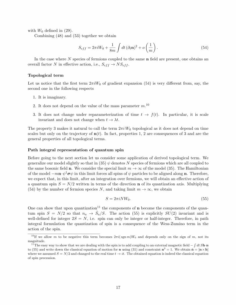
In the case where N species of fermions coupled to the same n field are present, one obtains anoverall factor N in effective action, i.e., Seff → NSeff .

Topological term

Let us notice that the first term 2πiW0 of gradient expansion (54) is very different from, say, thesecond one in the following respects

1. It is imaginary.

2. It does not depend on the value of the mass parameter m.10

3. It does not change under reparameterization of time t → f(t). In particular, it is scaleinvariant and does not change when t→ λt.

The property 3 makes it natural to call the term 2πiW0 topological as it does not depend on timescales but only on the trajectory of n(t). In fact, properties 1, 2 are consequences of 3 and are thegeneral properties of all topological terms.

Path integral representation of quantum spin

Before going to the next section let us consider some application of derived topological term. Wegeneralize our model slightly so that in (35) ψ denotes N species of fermions which are all coupled tothe same bosonic field n. We consider the special limit m→∞ of the model (35). The Hamiltonianof the model −mn·ψ†σψ in this limit forces all spins of ψ particles to be aligned along n. Therefore,we expect that, in this limit, after an integration over fermions, we will obtain an effective action ofa quantum spin S = N/2 written in terms of the direction n of its quantization axis. Multiplying(54) by the number of fermion species N , and taking limit m→∞, we obtain

S = 2πiNW0. (55)

One can show that upon quantization11 the components of n become the components of the quan-tum spin S = N/2 so that na → Sa/S. The action (55) is explicitly SU(2) invariant and iswell-defined for integer 2S = N , i.e. spin can only be integer or half-integer. Therefore, in pathintegral formulation the quantization of spin is a consequence of the Wess-Zumino term in theaction of the spin.

10If we allow m to be negative this term becomes 2πi( sgnm)W0 and depends only on the sign of m, not itsmagnitude.

11The easy way to show that we are dealing with the spin is to add coupling to an external magnetic field −∫dt Sh·n

to (55) and write down the classical equation of motion for n using (31) and constraint n2 = 1. We obtain n = [n×h]where we assumed S = N/2 and changed to the real time t→ it. The obtained equation is indeed the classical equationof spin precession.

17

3.3 Derivation of a WZ term from fermionic model without chiral rotation

Here we give an alternative derivation of an effective action (54) from (37) which does not use chiralrotation trick. [10]

Consider

Z =

∫DψDψDn e−S , (56)

where

S =

∫ T

0dt ψ (i∂t − imn · τ )ψ. (57)

Here ψ = (ψ1, ψ2) is a Grassmann spinor representing spin 1/2 fermion, τ are the Pauli matricesacting on spinor indices of ψ, and n2 = 1 is a unit, three-component vector coupled to the spin offermion ψτψ with the coupling constant m. Integrating out fermions in (56) we obtain

Z =

∫Dn e−Seff(n), (58)

withSeff(n) = − ln det (i∂t − imn · τ ) . (59)

Let us denote D = i∂t− imn · τ and D† = i∂t + imn · τ . We calculate the variation of the effectiveaction

δSeff = −TrδDD−1

= −Tr

δDD†(DD†)−1

= imTr

δn · τ (i∂t + imn · τ )(−∂2

t +m2 −mn · τ )−1

(60)

Expanding the fraction in n, calculating the trace, and keeping only lowest orders in n/m, weobtain:

δSeff =

∫dt

1

4mδn · n− i

2δn · [n× n]

. (61)

Restoring the effective action from its variation we have:

Seff =

∫ T

0dt

1

8mn2 − 2πiW0, (62)

where the Wess-Zumino action

W0 =

∫ 1

0dρ

∫ T

0dt

1

8πεµνn · [∂µn× ∂νn] . (63)

Here ρ is an auxiliary coordinate ρ ∈ [0, 1]. Also, the n-field is extended to n(t, ρ) in such a waythat n(t, 0) = (0, 0, 1) and n(t, 1) = n(t). Indices µ, ν take values t, ρ.

The Wess-Zumino action (63) has a very special property. Although it is defined as an integralover two-dimensional disk parameterized by ρ and t its variation depends only on the values of non the boundary of the disk—physical time.

18

3.4 Quantum spin as a particle moving in the field of Dirac monopole

Let us think of the action (62) as of the action of a charged particle moving on a surface of two-dimensional sphere with unit radius so that n is a position of particle on the sphere. Then thefirst term of (62) is a conventional kinetic energy of the particle. The second term should then beinterpreted as a phase picked by particle moving in the field a magnetic charge 2S (Dirac monopole)placed in the center of the sphere.

One could have started with the problem of particle of the mass m moving in the field ofmagnetic monopole of charge 2S. Then the ground state is 2S-degenerate and is separated by thegap ∼ 1/m from the rest of the spectrum. In the limit m→ 0 only the ground state is left and weobtain a quantum spin problem in an approach analogous to the plane rotator from Sec.2.4.

3.5 Reduction of a WZ term to a theta-term

Let us consider the value of (29) assuming that the polar angle is kept constant at θ(τ) = θ0. Then(29) becomes

W0 =1− cos θ0

2

∫ β

0

dτ

2π∂τφ, (64)

and we recognize (53) with (64) as the theta-term (12) corresponding to the particle on a ring withthe flux through the ring given by

A =1− cos θ0

2. (65)

In particular, θ0 = π/2 the topological term in the action of a particle on a ring in magnetic fieldA = 1/2.

3.6 Properties of WZ terms

WZ terms

1. do not depend on the metric of spacetime

2. are imaginary in Euclidean formulation

3. do not contribute to stress-energy tensor (and to Hamiltonian).

4. do not depend on m – the scale, below which an effective action is valid (but do depend onsgn (m))

5. are antisymmetric in derivatives with respect to different space-time coordinates (containεµνλ...)

6. are written as integrals of (D+1)-forms over auxiliary (D+ 1)-dimensional space - disk DD+1

such that ∂DD+1 = SD - compactified space-time

7. are multi-valued functionals. Multi-valuedness results in quantization of coupling constants(coefficients in front of WZ terms)

8. do change equations of motion by changing commutation relation between fields (Poisson’sbrackets), not by changing Hamiltonian

9. might lead to massless excitations with “half-integer spin” (see Sec. 4.5)

19

10. describe boundary theories of models with θ-terms (see Sec. 4.5)

11. being combined (see the spin chains Sec. 4.2) produce θ-terms

12. can be calculated by gradient expansion of the variation of fermionic determinants

13. produce θ terms as a reduction of target space (see the Sec. 3.5) [10]

Among the listed properties the first five 1-5 are the properties of all topological terms while theothers are more specific to WZ terms.

3.7 Exercises

The exercises (4-9) were solved in the main text. Try to solve them independently and test yourunderstanding by solving exercises (10-11).

Exercise 4: WZ term in 0 + 1, preliminaries

Consider a three-dimensional unit vector field n(x, y) (n ∈ S2) defined on a two-dimensional disk D. Define

W0 =

∫D

d2x1

8πεµνn · [∂µn× ∂νn] =

∫D

1

16πitr [ndndn], (66)

where the latter expression is written in terms of differential forms and n = n · σ.a) Calculate the variation of W0 with respect to n. Show that the integral becomes the integral over

disk D of the complete divergence (of the exact form).b) Parametrize the boundary ∂D of the disk by parameter t, apply Gauss-Stokes theorem and express

the result of the variation using only the values of n(t) at the boundary.We showed that the variation of W depends only on the boundary (i.e. physical) values of n-field. See

(31) for the answer.

Exercise 5: WZ term in 0 + 1, definition

Assume that we are given the time evolution of n(t) field (n ∈ S2). We also assume that time can becompactified, i.e. n(t = β) = n(t = 0). Consider the two-dimensional disk D which boundary ∂D isparametrized by time t ∈ [0, β]. The WZ term is defined by

SWZ = i4πSW0[n], (67)

where S is some constant, W0 is given by Eq. (66), and n(x, y) is some arbitrary smooth extension of n(t)from the boundary to an interior of the disk.

Let us show that the WZ term is well defined and (almost) does not depend on the extension of n(t) tothe interior of D.

Consider two different extensions n(1)(x, y) and n(2)(x, y) of the same n(t) and corresponding values

W(1)0 and W

(2)0 of the functional W0. Show that the difference W

(1)0 −W (2) is an integer number - the degree

Q of mapping S2 → S2. The second S2 here is a target space of n. How did the first S2 appear?We see that SWZ [n(t)] is a multi-valued functional which depends on the extension of n to the disk D.

However, the weight in partition function is given by e−SWZ and can be made single-valued functional if thecoupling constant S is “quantized”. Namely, if 2S ∈ Z (S - half-integer number) the e−SWZ is a well-definedsingle-valued functional.

For the answer see (32).

20

Exercise 6: WZ in 0 + 1, spin precession

Let us consider the quantum-mechanical action of the unit vector n(t) with the (Euclidean) action

Sh = SWZ [n(t)]− S∫dth · n(t), (68)

where SWZ is given by (67) and h is some constant three-component vector (magnetic field).Find the classical equation of motion for n(t) from the variational principle δSh = 0. Remember that

one has a constraint n2 = 1 which can be taken into account using, e.g., Lagrange multiplier trick.The obtained expression is the equation of spin precession and SWZ is a proper, explicitly SU(2) invariant

action for the free spin S.For the answer see (33,26).

Exercise 7: WZ in 0 + 1, quantization

Show that the classical equations of motion obtained from Sh correspond to Heisenberg equations (in real

time) ∂tS = i[H, S

]for the quantum spin operator S[

Sa, Sb]

= iεabcSc (69)

obtained from the Hamiltonian of a spin in magnetic field

H = −h · S. (70)

Obtain the commutation relations of quantum spin (69) from the topological part SWZ . Notice thatthis topological action is linear in time derivative and, therefore, does not contribute to the Hamiltonian.Nevertheless, it defines commutation relations between components of the spin operator.

Hint : You can either use local coordinate representation of the unit vector in terms of spherical angles n =(cosφ sin θ, sinφ sin θ, cos θ) or use the general formalism of obtaining Poisson bracket from the symplecticform given in SWZ .

Exercise 8: Reduction of the WZ-term to the theta-term in 0 + 1

Let us assume that the field n(t) is constrained so that it takes values on a circle given in spherical coordinatesby θ = θ0 = const. Find the value of the topological term SWZ on such configurations (notice that thisconstraint is not applicable in the interior of the disk D, only at its physical boundary). Show that theobtained topological term is a theta-term in 0 + 1 corresponding to S1 → S1.

What is the value of the coefficient in front of that topological term? What is the value of corresponding“magnetic flux” through a ring? For S = 1/2 which reduction (value of θ0) corresponds to the half of theflux quantum?

For the answer see Sec. 3.5.

Exercise 9: WZ in 0 + 1, derivation from fermions

Consider a Euclidean action of a fermion coupled to a unit vector

SE =

∫dτ ψ†Dψ, (71)

whereD = ∂τ −mn · τ , (72)

with n ∈ S2 and τ the vector of Pauli matrices. We obtain an effective action for n induced by fermions as

e−Seff =

∫DψDψ†e−SE = DetD, (73)

21

orSeff = − log DetD = −Tr logD. (74)

We calculate the variation of Seff with respect to n as

δSeff = −Tr δDD−1 = −Tr δDD†(DD†)−1, (75)

where D† = −∂τ −mn · τ . We have

DD† = −∂2τ +m2 −mn · τ = G−10 −mn · τ . (76)

Expand (75) in 1/m up to the term m0 and calculate functional traces. Show that the term of the orderm0 is a variation of the WZ term in 0+1 dimensions. Restore Seff from its variation. What is the coefficientin front of the WZ term? To what value of spin does it correspond?

For the answer see Sec. 3.3.

Exercise 10: Fermionic determinant in two dimensions

Let us consider two-dimensional fermions coupled to a phase field φ(x) (φ ≡ φ + 2π). The EuclideanLagrangian is given by

L2 = ψ[iγµ(∂µ − iAµ) + imeiγ

5φ]ψ, (77)

where µ = 1, 2 is a spacetime index, γ1,2,5 is a triplet of Pauli matrices, and Aµ is an external gauge fieldprobing fermionic currents.

We assume that the bosonic field φ changes slowly on the scale of the “mass” m. Then one can integrateout fermionic degrees of freedom and obtain an induced effective action for the φ-field as a functionaldeterminant.

Seff = − log DetD, (78)

D = iγµ(∂µ − iAµ) + im eiγ5φ. (79)

We calculate the effective action using the gradient expansion method. Namely, we calculate the variationof (78) with respect to the φ and A-fields and use

δSeff = −δ log DetD = −Tr δ logD = −Tr δDD−1 = −Tr δDD†(DD†)−1. (80)

a) Calculate DD† for (79). Observe that this object depends only on gradients of φ-field.b) Expand (DD†)−1 in those gradients. This will be the expansion in 1/m. (It is convenient to introduce

notation G−10 = −∂2µ +m2).c) Calculate functional traces of the terms up to the order of m0. Use the plane wave basis to calculate

the trace Tr (X)→∫d2x

∫d2p(2π)2 e

−ip·xXeip·x.

d) Identify the variation of the topological term in the obtained expression. It contains the antisymmetrictensor εµν and is proportional to sgn (m).

e) Remove the variation from the obtained expression and find Seff up to the m0 order.f) Which terms of the obtained action are topological? Can you write them in terms of differential forms?For the answer see Ref. [10].

Exercise 11: “Dangers” of chiral rotation

Try to calculate the determinant of the previous exercise using “chiral rotation trick”. Namely, considerchiral rotation ψ → e−iγ

5φ/2ψ. Then ψ† → ψ†eiγ5φ/2 and ψ → ψe−iγ

5φ/2. Use the identity γµγ5 = −iεµνγνand anti-commutativity of Pauli matrices to show that the operator D(Aµ, φ) transforms into

D(Aµ, φ) = e−iγ5φ/2D(Aµ, φ)e−iγ

5φ/2 = D(Aµ +i

2εµν∂νφ, 0) = D(Aµ, 0).

22

Try to calculate log Det D = log DetD(A, 0) using expansion in A. You will see that the result does notmatch the effective action obtained in the previous exercise. Why? What one should add to the chiralrotation trick to make the correct calculation?

Answer: The Jacobian of the change of variables corresponding to the chiral rotation. See Refs. [10] and[26].

4 Spin chains.

Here we study how topological terms appear in effective theories for quantum spin chains. Weemphasize an interplay between different types of topological terms and the effects of topologicalterms on field dynamics. In addition to original papers, the useful references for this section include:[6, 27, 9].

Let us start with the model of quantum magnet

H =∑<kj>

JkjSk · Sj −∑j

hj · Sj . (81)

Here the summation is taken over the sites k, j of some d-dimensional lattice, Jkj are exchangeintegrals and hj is an external (generally space and time-dependent) magnetic field. The quantumspin operators Si have SU(2) commutation relations (a, b, c = 1, 2, 3)[

Saj , Sbk

]= iδjkε

abcScj . (82)

Commuting the spin operator Saj with the Hamiltonian Eq. (81) one obtains Heisenberg equationof motion for the spin operator

∂tSj = i[H,Sj ] = −∑k

JjkSk × Sj + hj × Sj . (83)

4.1 Path integral for quantum magnets

Path integral for the magnet on a lattice

The classical action for the magnet (81,82) can be written as

S = −4πiS∑j

W0[nj ] +

∫dτ H , (84)

where we introduced classical unit vectors ni and summed the terms (63) for each spin. Theclassical Hamiltonian used in (84) is obtained from (81) substituting Si by Sni. Variation of theaction (84) over nj with the use of Eq. (31) produces classical equation of motion

− iS ∂τnj × nj + S2∑k

Jkjnk − S∑i

hj = 0 . (85)

Taking a cross-product with nj gives a classical analogue of (83)

− i∂τnj = S∑k

Jkjnk × nj −∑i

hj × nj . (86)

Remember that −i∂τ = ∂t.

23

The path integral over trajectories of unit vectors nj(τ) with the amplitude e−S correspondingto the classical action (84) gives the quantization corresponding to (81,82). Our goal now is to finda continuum quantum field theory description of this lattice magnet.

Here important remark is in order. A given lattice theory does not necessarily have a reasonablecontinuum description. One needs a special reason for continuum approximation to be applicable.Such reasons could be the vicinity to a second order phase transition where correlation lengthbecomes much bigger than the lattice spacing or some other reasons for scale separation. In thefollowing we will try to first derive a continuum limit for the theory and then check the self-consistency of the continuum approximation. Another important point is that the way to take acontinuum limit depends crucially on the state of the system. In the following we first consider theferromagnetic state and then go to the collinear antiferromagnetic state.

Continuum limit for Quantum Ferromagnet

Let us assume for simplicity that Jjk = J < 0 for nearest neighbor sites j, k of a spin chain in 1d,square lattice in 2d and cubic lattice in 3d and magnetic field is constant hj = h. The classicalHamiltonian is then

H = −|J |S2∑<kj>

nk · nj − S∑j

h · nj . (87)

We assume that there is a short range ferromagnetic order, i.e. nearest neighbor spins are almostperfectly aligned. We replace spins nj at lattice sites by a continuous field n(x) and proceed asfollows. Up to a constant, nj+ex · nj → −1

2(nj+ex − nj)2 → −1

2a2(∂xn)2 etc. Here a is the lattice

constant. Replacing the summation over j by the integration over space, we obtain the continuumlimit of the Hamiltonian (87)

H = −1

2|J |S2a2

∫ddx

ad(∂µn)2 − S

∫ddx

adh · n . (88)

Similarly, we have for the full action (84)

S[n] = −4πiS

∫ddx

adW0[n(x, τ)] (89)

− 1

2|J |S2a2

∫dτddx

ad(∂µn)2 − S

∫dτddx

adh · n .

Variation of this action with respect to the continuous unit vector field n(x, τ) produces the well-known classical Landau-Lifshitz equation for magnetization (to go to real time one should replacei∂τ → −∂t)

i∂τn = |J |Sa2 (n×∆n)− h× n . (90)

Let us remark here that W0[nj ] is a topological term for an individual spin nj on the site j of thelattice. However, due to the integration over space, the first term of the continuum action Eq. (89)depends on the spatial metric (e.g., distortions of the lattice will change it). Therefore, this termcannot be considered topological. Nevertheless, it is linear in time derivative and therefore time-reparameterization invariant. Therefore, it remains imaginary after Wick’s rotation and results ina very essential interference even in imaginary time path integral.

24

Bloch’s law: the dispersion of spin waves in ferromagnet

As an application of the continuum theory for magnetization in ferromagnets, let us derive thedispersion of spin waves starting from (90). We assume that magnetic field is constant and uniformh = (0, 0, h), and that there is a long range ferromagnetic order with spins oriented in the samedirection. We also assume that spin fluctuations are small and write n = (u1, u2, 1), where u1,2

are components of n in x, y directions in spin space that are assumed to be small so that n2 =1 + u2

1 + u22 ≈ 1 up to quadratic terms in u. Substituting all this in (90) we obtain

− iωu = −i|J |Sa2k2u− ihu . (91)

Here we introduced complex notation u = u1 + iu2 and made Fourier transform ∆ → −k2 andi∂τ → −∂t → iω. We immediately obtain the dispersion of spin waves

ω = |J |Sa2k2 + h , (92)

the result known as the Bloch’s law. In the absence of external magnetic field the dispersion ofspin waves is quadratic in wave vector k.

To conclude our brief discussion of the ferromagnetic case we have to recall that the continuumtheory was derived under the condition that fluctuations of n are small compared to 1 or |u| 1.Given a temperature and other parameters of the theory one should calculate the average value ofthose fluctuations. The condition 〈|u|2〉 1 is then the necessary condition for the self-consistencyof the continuum approximation.

4.2 Continuum path integral for Quantum Antiferromagnet

Let us consider a more subtle case of quantum antiferromagnet. We again start with the Hamilto-nian (87). However, we assume now that J > 0 and write

H = JS2∑<kj>

nk · nj − S∑j

h · nj . (93)

Although (93) looks very similar to (87) the unit vectors nj tend to be antiparallel on nearest sites(we again assume square lattice here so that the antiferromagnetic order is not frustrated). Onecannot use the continuous field n(x) instead of lattice vectors nj . Taking continuum limit is moreinvolved and can be achieved through the following substitution

nj = (−1)jm(x) + al(x) . (94)

Here we assume that both fields m(x) and l(x) are good continuous (smooth) fields. 12 The formerrepresents the smooth staggered magnetization while the latter is a ferromagnetic component. It isexpected that the ferromagnetic component is small and the corresponding rescaling by the latticeconstant a is made. As n2

j = 1 we have

n2j = m2 + 2(−1)ja(m · l) + a2l2 = 1 . (95)

We solve this condition to the order of a2 by two conditions

m2 = 1 , m · l = 0 . (96)

12We emphasize that in the following we take a particular continuum limit which assumes short range orderedantiferromagnetic state. It is believed to be appropriate for large S Heisenber antiferromagnets. However, it is notappropriate, e.g. for spin chains at so-called Bethe Ansatz integrable points.

25

Using (94) we have up to constants

nj+ex · nj →1

2a2[(∂xm)2 + 4l2 + 4(−1)j∂xm · l

],

h · nj → (−1)jh ·m + ah · l .

Substituting these expressions into (93) we obtain

H = JS2∑j

1

2a2[(∂µm)2 + 4dl2 + 4(−1)j∂µm · l

]− S

∑j

((−1)jh ·m + ah · l) .

→ JS2a2 1

2

∫ddx

ad[(∂µm)2 + 4dl2

]− Sa

∫ddx

adh · l . (97)

In the last step, we dropped all oscillating terms and replaced summation by integration over space.The next step is to do a similar procedure with the term in the action coming from the sum-

mation of topological terms. We proceed as follows∑j

W0[nj ] =∑j

W0[(−1)jm(x) + al(x)]

≈∑j

(−1)jW0[m(x) + (−1)jal(x)]

≈∑j

(−1)jW0[m(x)] +

∫ddx

ad

∫dτ al(x)

δW0[m]

δm

We now use the variation formula (31) and its consequence

W0[m(x+ ex)]−W0[m(x)] ≈ 1

4π

∫dτ (a∂xm) · (m× ∂τm)

and obtain ∑j

W0[nj ] ≈1

4π

∫ddx

ad

∫dτ ad l(x) · (m× ∂τm) (98)

+∑jy ,jz

(−1)jy+jz 1

8π

∫dx

a

∫dτ (a∂xm) · (m× ∂τm) .

The first term of (98) is written for any spatial dimension d. In the second term, we assumed thethree-dimensional case. Notice that while the sign alternation was taken into account in x directionthere is still a sum to be taken with the factor (−1)jy+jz in other two directions. That summationwill suppress this term and, therefore, it is relevant only in one spatial dimension. We summarizefor the topological contribution

−4πiS∑j

W0[nj ] ≈ −iSa1−dd

∫dτ ddx l(x) · (m× ∂τm)

− iS

2δd,1

∫dτ dx ∂xm · (m× ∂τm) . (99)

26

Collecting all terms together to get the continuum limit of the action (84) we obtain

S[m, l] = iS

2δd,1

∫dτ dx ∂xm · (m× ∂τm)− iSa1−dd

∫dτ ddx l(x) · (m× ∂τm)

+ JS2a2−d 1

2

∫dτ ddx

[(∂µm)2 + 4dl2

]− Sa1−d

∫dτ ddxh · l

= iS

2δd,1

∫dτ dx ∂xm · (m× ∂τm) + JS2a2−d 1

2

∫dτ ddx (∂µm)2

+

∫dτ

ddx

ad

(2JS2a2dl2 − Sa1l ·

[h + id (m× ∂τm)

]). (100)

The obtained expression is the continuum limit of (84) derived in the antiferromagnetic regimewith the assumption of small fluctuations around the short range collinear antiferromagnetic order.The field l describing the magnetization of the magnet enters the action in a very simple way andcan be “integrated out”. For details of derivation see the Appendix B. Here we present the resultsdropping the external magnetic field for simplicity. In two and higher spacial dimensions d > 1, wehave

S[m] =1

2g

∫dτ

ddx

ad−1

[1

vs(∂τm)2 + vs(∂µm)2

], (101)

where

vs =2JSa√

d, g =

2

S√d. (102)

The one-dimensional case is special and has an additional topological term in the action

S[m] =1

2g

∫dτ dx

[1

vs(∂τm)2 + vs(∂xm)2

]+ iθ

∫dτ dx

1

4πm · (∂τm× ∂xm) , (103)

where

vs = 2SaJ , g =2

S, θ = 2πS . (104)

The model (103) is known as O(3) nonlinear sigma model with topological theta-term. It is thelow energy, long distance description of the antiferromagnetic Heisenberg spin chain with largespin S 1 with the correspondence between parameters of the model and the parameters of thespin chain given by (104). Let us start with the discussion of the nonlinear sigma model withouttopological term.

4.3 RG for O(3) NLSM

The model, Eq. (103) without topological term (θ = 0) can be re-written as

S[m] =1

2g

∫d2x (∂µm)2 , (105)

where µ = τ, x and we re-defined τ → τ/vs. The action (105) with the constraint m2 = 1 is knownas O(3) nonlinear sigma model (NLSM). It is relativistically invariant with spin wave velocityvs playing the role of the speed of light. This relativistic invariance is emergent and we should

27

remember that the next order gradient corrections to the model and various perturbations aregenerally not relativistically invariant.

At small values of the coupling constant g corresponding to large values of S one can treat (105)perturbatively and ask how the coupling constant renormalizes when one goes to longer distances.It turns out [28] that g increases with the scale. The increase of g signals the tendency of the m-fieldto disorder. More precisely, the effective coupling of (105) at the length L satisfies renormalizationgroup (RG) equation

dg

d logL=

1

2πg2 +O(g3) , (106)

and gives

g(L) =g0

1− g0

2π log(L/a), (107)

where g0 = g(a) is the coupling constant at UV (lattice) scale a. At the scale L ∼ ξ with

ξ ∼ ae2π/g0 , (108)

the effective coupling constant g(ξ) becomes of the order of unity and we cannot trust RG equation(106) at this point.

We stress here that RG analysis is not conclusive. The only conclusion we can make is that theeffective length ξ given by (108) emerges. At this scale, the m field is somewhat disordered, but wecannot say anything about the nature of the phase and about the long distance behavior of m-fieldcorrelation functions. There are essentially two scenarios. The first one is that the actual modelhas a gap of the order of vs/ξ, the field m is disordered with all correlations decaying exponentiallywith the correlation length ξ (108). The second possibility is that the RG flow leads to a newfixed point and behavior of the model at scales larger than ξ is governed by that fixed point (inparticular, long range correlation functions might decay as power laws etc.). It turns out that thisis the former scenario that is realized for 2d O(3) nonlinear sigma model (105). We know thisbecause O(3) NLSM has been solved exactly by Bethe Ansatz [29] and has a gap separating theground state from excitations. In the next section we will argue that the second scenario might berelevant when topological term is present in NLSM.

Bethe Ansatz solution of the model (105) is outside of the scope of these lectures. Instead,to have some understanding of how finite gap (correlation length) appears in NLSM we refer thereader to the Exercise 13 “O(N) NLSM” below where the correlation length is obtained for theO(N) NLSM in the limit of large N .

4.4 O(3) NLSM with topological term

Let us now consider the O(3) NLSM with topological theta term

S[m] =1

2g

∫d2x (∂µm)2 + iθQ , (109)

where

Q =

∫d2x

1

4πm · (∂τm× ∂xm) . (110)

We assume that the boundary conditions m(x) → m0 = const, as x → ∞ so that the windingnumber Q is an integer. The parameters corresponding to the AFM spin chain are given by(103,104), i.e., g = 2/S and θ = 2πS. Following Haldane [30, 31], we notice that the topological

28

term in (109) contributes the complex weight to path integral given by eiθQ = (−1)2SQ. Thisweight depends crucially on the integer-valuedness of spin. If the spin S is half-integer, the weightis non-trivial (−1)Q and results in interference of topological sectors characterized by differenttopological charges Q. On the other hand, if S is integer, the weight is unity and does not affectthe path integral. 13 Based on this observation Haldane conjectured that AFM spin chains withinteger spin S have singlet ground states separated by finite gap from all excitations similar to O(3)NLSM without topological term. On the other hand, AFM spin chains with half-integer spin havegapless excitations similar to the spin-1/2 chain. For the latter, the spectrum of excitations hasbeen known from the exact solution by Bethe [32]. The Haldane’s conjecture has been supportedby numerical simulations and experiments.

It is instructive to think about RG flow for the NLSM with theta term. The model has twoparameters g and θ and it is appealing to think about RG flow in the plane labeled by thoseparameters. First of all, we notice that starting with dimerized spin chain one obtains values of θwhich are not necessarily multiples of π (see Exercise 12 “Dimerized spin chain” below). Therefore,it is tempting to draw the flow diagram similar to the one for integer quantum Hall effect [33, 34](see figure 4).

It is not difficult to see that conventional perturbative calculation results in non-renormalizabilityof θ. This is reflected by strictly vertical flow at small g (large 1/g) in figure 4. One can arguefollowing [33] that taking into account instanton configurations (configurations with Q 6= 0) willresult in the deviations of flow from the vertical one as shown in the figure. However, the instantoncontribution is suppressed by factors of the order of e−2π/g and it is very hard to develop consistentperturbation theory taking into account exponentially small terms but neglecting terms of higherorder in coupling g. More straightforward interpretation of figure 4 is that it shows the flow of someobservables which correspond to 1/g and θ at small values of g and change with scale as shown inthe figure (in analogy with observable conductances σxx and σxy of [33]). We will not dwell on theinterpretation of figure (4). However, it is believed that as shown on that figure the long distancebehavior of spin chains of half-integer θ/(2π) is governed by new infrared fixed points while the spinchain with any other θ flows to the models with finite gap in the spectrum. In fact, it was clarifiedthat the critical description of half-integer spin chains is given by Wess-Zumino-Witten (WZW)model (see Ref. [35]). In particular, the staggered magnetization correlation decays as power lawat large distances.

In the limit of large S, we have the following picture for the correlator 〈m(x)·m(0)〉. At distancesshorter than ξ ∼ aeπS (obtained form (108) at g = 2/S) there is a short range antiferromagneticorder 〈m(x) · m(0)〉 ∼ 1. At larger distances x ξ, the order is destroyed, and there is nolong-range order in agreement with the Mermin-Wagner theorem. However, the way in whichcorrelations decay at large distances depend crucially on S. If S is integer, the decay is exponential〈m(x) ·m(0)〉 ∼ e−x/ξ, while at half-integer S, it is algebraic (power-law) with 〈m(x) ·m(0)〉 ∼ x−1.14 This power-law signals the emergent scale invariance (in fact, conformal invariance) and iscaptured by the infrared fixed point of effective WZW model. Interestingly, for half-integer spinsthe symmetry of the spin chain is enlarged at the critical point. In addition to the fluctuations ofthe staggered magnetization m(x), fluctuations of dimerization become soft as well. They combineinto the effective SU(2) “order parameter” which is an SU(2) degree of freedom of WZW model.We refer the reader to [35] for more detailed analysis of critical behavior of spin chains.

13This statement is not quite correct. The topological term can still be important for various boundary conditionsand due to the presence of singularities.

14At non-zero temperature there is another length scale ξT ∼ aJS2/T , and power-law decay of correlations will beeventually replaced by exponential decay at large distances due to thermal fluctuations.

29

0 1 2

1/g

1/2 3/2θ/2π

Figure 4: The schematic RG flow for nonlinear sigma model with theta term is shown. The verticalaxis is the inverse coupling constant g while the horizontal axis is the topological angle θ. Thepicture has exact symmetry with respect to θ → θ + 2π and with respect to reflection relative tohalf integer θ/2π. The horizontal dashed line corresponds to g ∼ 1. Below this line the perturbativeRG is not working and interpretation of the flow is more subtle.

30

4.5 Boundary states for spin 1 chains with Haldane’s gap

We argued at the beginning of Sec. 4.4 that for integer S the topological term is “ineffective” andthe model (109) behaves similarly to the O(3) NLSM without topological term (105). This is notquite correct. The argument is essentially based on the integer-valuedness of the topological chargeQ. However, it is necessarily integer only for smooth m-field configurations for compact boundaryconditions (e.g., m→m0 at x, t→∞). Let us consider an example when boundary conditions aredifferent.

We assume that the spin chain is long but has a finite length L with free boundary conditions(boundary spins at x = 0, L can take arbitrary values). Then the topological term can be writtenas

Stop[m] = iθ

∫dτ

∫ L

0dx

1

4πm · (∂τm× ∂xm)

= iθ

[ΩL

4π+Q− Ω0

4π

]. (111)

Here we decomposed the winding number (110) into integer part Q and the difference of solid anglesΩ0,ΩL subtended by boundary vectors m(0) and m(L), respectively. Assuming θ = 2π, we dropthe integer part and end up with the contribution

Stop = i

[ΩL

2− Ω0

2

], (112)

which is written in terms of boundary vectors only. Comparing with (29) we recognize (112) as theaction of two spin-1/2 located at the ends of the spin chain. As we expect that the bulk degrees offreedom have a gap in the spectrum (S = 1 is an integer) we conclude that the S = 1 AFM spinchain in the gapful phase (Haldane’s phase) should have gapless boundary spin 1/2 excitations.

We would like to stress again how unusual is the conclusion we have just made. It is well knownthat “adding” finite number of spin 1s one can get only superposition of integer valued spins. Forexample, two spin-1 particles can only have sectors with total spins 0, 1, and 2. However, wemanaged adding large number of spin 1s to get two boundary spin 1/2 as low lying excitations ofthe finite spin chain with free boundary conditions! 15 Most amazingly, these boundary spin 1/2have been observed in experiment. [36, 37]

This example illustrates very interesting connection between θ and WZW topological terms.The gapful model with θ terms might produce massless boundary theory of one dimension lowerdescribed with the use of WZ terms.

4.6 AKLT model

To understand better how the bulk gap and boundary spin 1/2 states are formed in the Haldane’sphase of S = 1 antiferromagnetic spin chain let us consider the deformation of the HeisenbergHamiltonian known as AKLT model [38, 39]

H = J∑j

(Sj · Sj+1 +

1

3(Sj · Sj+1)2

). (113)

15Actually, for the finite length of the spin chain those two boundary spin 1/2 are effectively interacting with thestrength of interaction ∼ e−L/ξ. Only in the limit of an infinite length we obtain truly non-interacting spin 1/2degrees of freedom.

31

mm

m

L

0

Figure 5: Time evolution of boundary magnetizations (unit vectors) m0(τ) and mL(τ) is shown.For periodic time these vectors sweep solid angles Ω0 and ΩL, respectively. The shaded area isgiven by (111) which is up to integer Q is given by the difference of solid angles ΩL and Ω0 as in(112).

One should think about this model as fine tuned model with the coefficient J ′ in front of thebiquadratic term being exactly 1/3 of the coefficient in front of Heisenberg exchange term. ChangingJ ′ from 0 to J/3 interpolates between Heisenberg spin chain and AKLT model (113). It can beshown that the ground state of (113) is separated by the finite gap from excitations. If this gap isnot closed in the process of changing J ′ from J/3 to zero then the Heisenberg spin chain has a gapas well and we say that AKLT and Heisenberg model are adiabatically connected and are in thesame phase.

Let us now see why AKLT model is much easier to analyze than the Heisenberg model forS = 1. It turns out that the Hamiltonian (113) up to constant can be written as

H = 2J∑j

P2(Sj + Sj+1) , (114)

where

P2(S1 + S2) =1

2Sj · Sj+1 +

1

6(Sj · Sj+1)2 +

1

3(115)

is a projector on the state with the total spin S = 2 (see the Exercise 15 “Projector to S = 2”).Then schematically (see [38, 39] for details) one can think about the ground and excited states of(114) in the following way. We split every spin Sj into two spins 1/2 (let us call them A and B.Taking one of those two spin 1/2 from the site j and one of spin 1/2 from the site j + 1 we form asinglet state and make a product of all these singlets. Then we project the result back to the totalspin 1 on each site. The obtained state

P∏j

(|+〉j,A|−〉j+1,B − |−〉j,A|+〉j+1,B

)

32

1 2 L

Figure 6: The schematic picture of the ground state of AKLT model. Ovals represent the sites ofthe spin chain. Spin 1 at each site is split in two spin 1/2s. The horizontal segments representsinglet states of spin 1/2-s from neighbor sites. Notice that one of spin 1/2-s at the site 1 and atthe site L are not parts of singlets. They are the boundary spin 1/2 states of the AKLT spin 1chain.

has a property that the sum of two neighbor spins is never 2 and is, therefore, the ground stateof (114) and of (113). 16 It is also physically clear that to excite this system one should breakone of the singlets and pay finite energy. Schematically we illustrate the construction in figure 6.In particular, one can see that the boundary spin 1/2 in this case are just uncoupled “halves” ofthe end spins of the chain. In some sense AKLT provides a “chemical” model with singlets beingcovalent bonds and spin 1/2-s being physical electrons. We refer to AKLT model as to a strongcoupling limit of the Haldane’s phase of a spin-1 chain.

4.7 Exercises

Exercise 12: Dimerized spin chain

Start with the spin-chain Hamiltonian

H =∑k

Jk Sk · Sk+1

with Jk = J > 0 if k even and Jk = J ′ > 0 if k odd. Repeat the derivation of the section 4.2 and show thatthe continuum limit is still given by O(3) NLSM with theta term (103) but instead of (104) the parametersof the model are given by

vs = 2Sa√JJ ′ , g =

1

S

(√J

J ′+

√J ′

J

), θ = 2πS

[1− J − J ′

J + J ′

]. (116)

Notice that the model is self-dual with respect to the duality transformation J ↔ J ′, θ → 4πS − θ corre-sponding to the reflection symmetry of the 1d lattice and the Hamiltonian.

Exercise 13: O(N) NLSM

Let us consider the model given by the action (105), where the unit vector field m2 = 1 has N componentsm = (m1,m2, . . . ,mN ). This model is known as O(N) nonlinear sigma model. We replace (105) by

S[m, λ] =1

2g0

∫d2x

[(∂µm)2 + iλ(m2 − 1)

]. (117)

We introduce here the field λ(x, t) so that functional integration over it gives the local constraint m2 = 1.Assuming that the functional integral over λ(x, t) is performed exactly one should not worry about the

16Of course, these speculations are not rigorous at all. For rigorous treatment see [38, 39] or modern treatmentusing the technique of matrix product states (MPS).

33

constraint in (117). Let us now make an approximation assuming that the functional integral correspondingto (117) is dominated by the saddle point iλ = M2 = const. Then the path integral over m is Gaussian.17

Compute this Gaussian integral and find 〈m2〉 for a given M . Assume that all divergent integrals canbe cut off by the lattice scale a. Write down the consistency equation 〈m2〉 = 1. This is the so-called gapequation which determined the saddle point value of M . Show that it is given by

M ∼ 1

aexp

(− 4π

Ng0

). (118)

Consider now fluctuations of λ around the saddle point, and show that these fluctuations are suppressed bythe parameter 1/N , i.e. one needs large N limit to make saddle point approximation self-consistent.

As a result of this exercise we obtained that the correlation functions of m-field behave as the ones forthe field with the mass M given by (118), i.e., 〈m(x) ·m(0)〉 ∼ exp(−Mx).

For the answer to this exercise see [6].

Exercise 14: Boundary spin 1/2 states of a Haldane’s chain

Consider the “action” of a two-dimensional O(3) non-linear sigma model with topological term

S = SNLSM + Sθ , (119)

SNLSM =1

2g

∫d2x (∂µn)2 , (120)

Sθ = iθQ , (121)

Q =

∫d2x

1

8πεµνn[∂µn× ∂νn] . (122)

This action can be derived as a continuum limit of the Heisenberg spin chain with large spins on sites. Inthe latter case, g = 2/S and θ = 2πS. In the case of integer S, the spin chain is massive, and there are nobulk excitations at low energies (smaller than the gap).

Let us assume that the action (119) is defined on the open chain of the length L. Show that thetopological theta-term (121,122) formally defined on the open chain reduces to two WZ (0+1-dimensional)terms at the boundary of spacetime, i.e. at the ends of the spin chain. This means that we expect twoquantum spins living at the ends of the spin chain. Show that the coefficient in front corresponds to thevalue of those spins S/2. In particular, it means that the boundary states of S = 1 spin chain correspond tospin-1/2!

Remark : Neglecting the NLSM part of the action is possible in this exercise only because of the gap inthe bulk at the integer value of spin.

For the answer see Sec. 4.5.

Exercise 15: Projector to S = 2

Show that the operator (115) projects any state of two spins S = 1 onto the state with total spin S = 2.Hint: use the identity (S1 · S2) = 1

2

[(S1 + S2)2 − 4

]for two spin-1 operators S2

1 = S22 = S(S + 1) = 2.

5 Conclusion

In these lectures, we considered a few examples of topological terms that appear in effective actionsused in condensed matter theory. We discussed some of the properties of those terms and theirphysical consequences. We also showed how these terms can be generated by fermionic degreesof freedom as phases of fermionic determinants. Of course, these lectures can serve only as anintroduction to a quickly developing field of topological phases of matter. Because of limited time we

17At this step we essentially replace the local constraint m2 = 1 for the global one∫d2xm2 = const and hope that

fluctuations of local magnitude of m are not important.

34

focused on topological terms in sigma-models and did not consider the ones made out of backgroundand dynamic gauge fields. The latter are related to the physics of quantum Hall effect (see [40] forsome recent developments) and to the physics of topological insulators and superconductors (e.g.,see [41]). Other interesting but much less understood topics include topological terms for singularprocesses (defects in space-time configurations, such as monopoles, hedgehogs and vortices), therole of topology for phases with gapless fermions, topology and physics out of equilibrium etc. Myhope is that these lectures were stimulating enough to encourage the reader to study and to workon applications of topology to physics.

6 Acknowledgements

I was inspired to work on topological terms in condensed matter physics by Paul Wiegmann. I havelearned most of what is written in these lectures working with Paul and I am infinitely grateful tohim for this experience. I would also like to thank Patrick Lee who encouraged my first attemptto lecture on topological terms at MIT. Some of these lectures were shaped in the “Topics” courseon topological terms for Stony Brook University’s physics graduate students. I thank all studentsand faculty attending those lectures for their attention and questions and to Paul Wiegmann andArtem Abanov for reading the manuscript and providing a very useful feedback. Finally, thesenotes would never be finished without Somen Bhattacharjee who invited me to SERC School onTopology and Condensed Matter Physics (2015, Kolkata, India) to give these lectures and gentlybut constantly reminded me to work on the notes.

References

[1] Robert B Laughlin and David Pines. The theory of everything. Proceedings of the NationalAcademy of Sciences of the United States of America, pages 28–31, 2000.

[2] Philip W Anderson et al. More is different. Science, 177(4047):393–396, 1972.

[3] Michael E Peskin and Daniel V Schroeder. Quantum field theory. The Advanced Book Program,Perseus Books Reading, Massachusetts, 1995.

[4] Murray Gell-Mann and Maurice Levy. The axial vector current in beta decay. Il NuovoCimento (1955-1965), 16(4):705–726, 1960.

[5] Stephen L Adler and Roger F Dashen. Current algebras and applications to particle physics,volume 30. Benjamin, 1968.

[6] A. M. Polyakov. Gauge Fields and Strings. CRC, September 1987.

[7] N David Mermin. The topological theory of defects in ordered media. Reviews of ModernPhysics, 51(3):591, 1979.

[8] Alexander Altland and Ben D Simons. Condensed matter field theory. Cambridge UniversityPress, 2010.

[9] Eduardo Fradkin. Field theories of condensed matter physics. Cambridge University Press,2013.

[10] AG Abanov and Paul B Wiegmann. Theta-terms in nonlinear sigma-models. Nuclear PhysicsB, 570(3):685–698, 2000.

35

[11] Alexander G Abanov. Hopf term induced by fermions. Physics Letters B, 492(3):321–323,2000.

[12] Frank Wilczek and Alfred Shapere. Geometric phases in physics, volume 5. World Scientific,1989.

[13] Sam Treiman and Roman Jackiw. Current algebra and anomalies. Princeton University Press,2014.

[14] BA Dubrovin, AT Fomenko, and SP Novikov. Modern geometry - methods and applications:Part II: The geometry and topology of manifolds, volume 104. Springer Science & BusinessMedia, 2012.

[15] Mikio Nakahara. Geometry, topology and physics. CRC Press, 2003.

[16] Michael Monastyrsky. Topology of gauge fields and condensed matter. Springer Science &Business Media, 2013.

[17] Vladimir I Arnold. Mathematical methods of classical mechanics. translated from the 1974russian original by k. vogtmann and a. weinstein. corrected reprint of the second (1989) edition.Graduate Texts in Mathematics, 60:229–234, 1991.

[18] Michael Stone and Paul Goldbart. Mathematics for physics: a guided tour for graduate stu-dents. Cambridge University Press, 2009.

[19] LD Landau and EM Lifshitz. Mechanics, vol. 1. Course of theoretical physics, pages 84–93,1976.

[20] Julius Wess and Bruno Zumino. Consequences of anomalous ward identities. Physics LettersB, 37(1):95–97, 1971.

[21] Edward Witten. Global aspects of current algebra. Nuclear Physics B, 223(2):422–432, 1983.

[22] S. P. Novikov. The hamiltonian formalism and a many-valued analogue of morse theory.Russian mathematical surveys, 37(5):1–56, 1982.

[23] Edward Witten. Current algebra, baryons, and quark confinement. Nuclear Physics B,223(2):433–444, 1983.

[24] Michael Stone. Born-oppenheimer approximation and the origin of wess-zumino terms: Somequantum-mechanical examples. Physical Review D, 33(4):1191, 1986.

[25] Edward Witten. An su(2) anomaly. Physics Letters B, 117(5):324–328, 1982.

[26] Kazuo Fujikawa and Hiroshi Suzuki. Path integrals and quantum anomalies. Number 122.Oxford University Press on Demand, 2004.

[27] Ian K Affleck. Field theory methods and quantum critical phenomena. Technical report,PRE-31353, 1988.

[28] Alexander M Polyakov. Interaction of goldstone particles in two dimensions. applications toferromagnets and massive yang-mills fields. Physics Letters B, 59(1):79–81, 1975.

[29] PB Wiegmann. Exact solution of the o (3) nonlinear σ-model. Physics Letters B, 152(3-4):209–214, 1985.

36

[30] FDM Haldane. Nonlinear field theory of large-spin heisenberg antiferromagnets: semiclassi-cally quantized solitons of the one-dimensional easy-axis neel state. Physical Review Letters,50(15):1153, 1983.

[31] F Duncan M Haldane. Continuum dynamics of the 1-d heisenberg antiferromagnet: identifi-cation with the o (3) nonlinear sigma model. Physics Letters A, 93(9):464–468, 1983.

[32] Hans Bethe. Zur theorie der metalle. Zeitschrift fur Physik, 71(3-4):205–226, 1931.

[33] Herbert Levine, Stephen B Libby, and Adrianus MM Pruisken. Electron delocalization by amagnetic field in two dimensions. Physical review letters, 51(20):1915, 1983.

[34] DE Khmel’nitskii. Quantization of hall conductivity. JETP lett, 38(9), 1983.

[35] Ian Affleck and FDM Haldane. Critical theory of quantum spin chains. Physical Review B,36(10):5291, 1987.

[36] Masayuki Hagiwara, Koichi Katsumata, Ian Affleck, Bertrand I Halperin, and JP Renard.Observation of s= 1/2 degrees of freedom in an s= 1 linear-chain heisenberg antiferromagnet.Physical review letters, 65(25):3181, 1990.

[37] M Kenzelmann, G Xu, IA Zaliznyak, C Broholm, JF DiTusa, G Aeppli, T Ito, K Oka, andH Takagi. Structure of end states for a haldane spin chain. Physical review letters, 90(8):087202,2003.

[38] Ian Affleck, Tom Kennedy, Elliott H Lieb, and Hal Tasaki. Rigorous results on valence-bondground states in antiferromagnets. Physical review letters, 59(7):799, 1987.

[39] Ian Affleck, Tom Kennedy, Elliott H Lieb, and Hal Tasaki. Valence bond ground states inisotropic quantum antiferromagnets. In Condensed Matter Physics and Exactly Soluble Models,pages 253–304. Springer, 1988.

[40] Andrey Gromov, Gil Young Cho, Yizhi You, Alexander G Abanov, and Eduardo Fradkin.Framing anomaly in the effective theory of the fractional quantum hall effect. Physical reviewletters, 114(1):016805, 2015.

[41] Shinsei Ryu, Joel E Moore, and Andreas WW Ludwig. Electromagnetic and gravitationalresponses and anomalies in topological insulators and superconductors. Physical Review B,85(4):045104, 2012.

[42] Kiyosi Ito. Encyclopedic dictionary of mathematics, volume 1. MIT press, 1993.

37

A Appendix: Topological defects and textures

In this appendix we collect few exercises on the topic of homotopy classifications of topologicaldefects and textures in media with spontaneously broken symmetry. A detailed exposure of thetopic could be found in the classic reference [7]. Some of known homotopy groups for various spacesare collected in Appendix C.

Exercise 16: Nematic

Nematic is a liquid crystal characterized by an order parameter which is the unit three-component vectorn = (n1, n2, n3), n2 = 1 with an additional condition n ∼ −n. The latter means that two unit vectors whichare opposite to each other describe the same state. Such an order parameter is called “director”.

What are the types of topological defects and textures allowed for three-dimensional nematic? Whatabout two-dimensional one?

Exercise 17: Crystal

One can view a crystalline state as a continuous translational symmetry broken to the subgroup of discretetranslations. Then the order parameter space should be identified (for three-dimensional crystal) withM = G/H = R3/(Z × Z × Z).

a) What (geometrically) is the order parameter space for this system?

b) What are the homotopy groups of this manifold π0,1,2,3(M) ?

c) What types of topological defects and textures are allowed in such a system?

Exercise 18: Superfluid 3He−AThe order parameter of superfluid 3He−A can be represented by two mutually orthogonal unit vectors ∆1,∆2. That is, at each point in three-dimensional space one has a pair of vectors with properties ∆2

1 = ∆22 = 1

and ∆1 ·∆2 = 0.

a) What is the order parameter space for this system?

b) What are the homotopy groups of this manifold π0,1,2,3(M) ?

c) What are the types of topological defects and textures allowed in such a system?

Exercise 19: Heisenberg model

What topological defects and textures should one expect in the ordered state of a three-dimensional classicalHeisenberg model? What changes if the order parameter is a director instead of a vector? A “director”means a vector without an arrow, i.e., one should identify S ≡ −S. The models with a director as an orderparameter are used to describe nematic liquid crystals (see Ex. 16).

Exercise 20: Continuum limit of XY model

Let us start with the XY model defined on a cubic d-dimensional lattice. The allowed configurations areparameterized by a planar unit vector ni = (cos θi, sin θi) on each site i of the lattice. The energy is givenby

E = −∑〈ij〉

J cos(θi − θj) . (123)

We assume that the most important configurations are smooth on a lattice scale and one can think of θi asof smooth function θ(x) defined in Rd - continuous d-dimensional space. Show that the energy is given inthis continuous limit by

E =J

2

∫ddx

ada2(∂µθ)

2 , (124)

38

where a is the lattice constant. The combination ρ(0)s = Ja2−d is referred to as bare spin-wave stiffness (or

bare superfluid density).Compute the energy of the vortex in such a model. Remember that the divergent integrals should be

cut off by lattice constant a and by the size of the system L at small and large distances, respectively.For the answer see Ref. [6].

Exercise 21: Correlation function 〈(θ(x)− θ(0))2〉Calculate the correlation function 〈(θ(x)− θ(0))2〉 in the XY model in d dimensions neglecting the topologyof θ, i.e., neglecting vortices and thinking about θ as of real number without periodicity. Divergencies atsmall distances should be cut off by the lattice constant a.

Hint: consider∫ddq e

iq·x

q2 with proper cutoffs. For the answer see Ref. [6].

Exercise 22: Correlation function 〈n(x) · n(0)〉. Low temperatures.

Using the result of the previous exercise calculate the correlation function 〈n(x) · n(0)〉 in the XY model ind dimensions neglecting the topology of θ. Write 〈n(x) · n(0)〉 = 〈cos(θ(x) − θ(0))〉 = Re 〈ei(θ(x)−θ(0))〉 anduse the properties of Gaussian integrals.

Make the conclusion about the existence of a true long range order in XY model in 2d and relate it tothe Mermin-Wagner theorem.

For the answer see Ref. [6].

Exercise 23: Correlation function 〈n(x) · n(0)〉. High temperatures.

Let us consider high temperatures. Assume that J/T 1. Using high temperature expansion for XY-model(123) show that correlation function 〈n(x) · n(0)〉 decays exponentially. Find the correlation length at hightemperatures.

For the answer see Ref. [6].

Exercise 24: Vortex unbinding

Make an estimate of the BKT phase transition temperature in 2d XY model. Use the energy of the vortexcalculated previously, the estimate of the entropy of the vortex, and the condition F = 0 for the free energyof the vortex.

For the answer see Ref. [6].

B Appendix: Integrating out l field

Consider the l dependent part of the action (100)∫dτ

ddx

ad

(2JS2a2d (l)2 − Sa1l ·

[h− λm + id (m× ∂τm)

]). (125)

Here we added the Lagrange multiplier λ. The variation with respect to λ produces the constraintl ·m = 0. The field l enters the action quadratically and can be integrated out just by substituting lgiven by the variational principle. After adding the Lagrange multiplier we can vary over l withoutany constraints and obtain

4JS2a2−dd l− Sa1−d[h− λm + id (m× ∂τm)

]= 0

or

l =1

4JSad

[h− λm + id (m× ∂τm)

].

39

Substituting the latter expression into (125) we obtain

1

8Jadd

∫dτ ddx

[h− λm + id (m× ∂τm)

]2. (126)

Variation over λ gives

0 = m ·[h− λm + id (m× ∂τm)

]= m · h− λ

which determines λ = h ·m and gives for the (126)

− 1

8Jadd

∫dτ ddx

[h−m(h ·m) + id (m× ∂τm)

]2

= − 1

8Jadd

∫dτ ddx

[h2 − (h ·m)2 − d2 (m× ∂τm)2 − 2idh · (m× ∂τm)

]→ 1

8Jad

∫dτ ddx

[d (∂τm)2 + 2ih · (m× ∂τm)

]. (127)

In the last step we dropped terms independent of m and the term quadratic in h. Putting allresults together, we obtain the effective action which is the functional of the m field only.

S[m] = iS

2δd,1

∫dτ dxm · (∂τm× ∂xm)

+ JS2a2−d 1

2

∫dτ ddx (∂µm)2 +

d

8Jad

∫dτ ddx (∂τm)2

+ i1

4Jad

∫dτ ddxh · (m× ∂τm) .

C Appendix: Homotopy groups often used in physics

In this appendix, we collect some of the homotopy groups often used in physics. Many of thesegroups can be found in [42].

Generalities

If M and N are two topological spaces then for their direct product we have

πk(M ×N) = πk(M)× πk(N) .

If M is a simply-connected topological space (π0(M) = π1(M) = 0) and group H acts on M thenone can form topological space M/H identifying points of M which can be related by some elementof H (x ≡ hx). Then we have the following relation

π1(M/H) = π0(H) .

In particular, if H is a discrete group, π0(H) = H, and

π1(M/H) = H .

For higher homotopy groups, we have the relation

πk(M/H) = πk(M), if πk(H) = πk−1(H) = 0 . (128)

40

Homotopy groups of spheres

For a circle

π1(S1) = Z,

πk(S1) = 0, for k ≥ 2.

For higher-dimensional spheres, it is true that

πn(Sn) = Z,

πk(Sn) = 0, for k < n.

Homotopy groups of spheres πn+k(Sn) do not depend on n for n > k + 1 (homotopy groups

stabilize). In the table below we show in bold face the cell from which homotopy groups remainstable (constant along the diagonal of the table).

Homotopy groups of spheres

π1 π2 π3 π4 π5 π6 π7 π8 π9

S1 Z 0 0 0 0 0 0 0 0

S2 0 Z Z Z2 Z2 Z12 Z2 Z2 Z3

S3 0 0 Z Z2 Z2 Z12 Z2 Z2 Z3

S4 0 0 0 Z Z2 Z2 Z × Z12 Z2 × Z2 Z2 × Z2

S5 0 0 0 0 Z Z2 Z2 Z24 Z2

S6 0 0 0 0 0 Z Z2 Z2 Z24

S7 0 0 0 0 0 0 Z Z2 Z2

S8 0 0 0 0 0 0 0 Z Z2

Here and thereon we denote by Z the group isomorphic to the group of integer numbers withrespect to addition. Zn is a finite Abelian cyclic group. It can be thought of as a group of n-throots of unity with respect to a multiplication. Alternatively, it is isomorphic to a group of numbers0, 1, 2, . . . , n− 1 with respect to addition modulo n. Or simply Zn = Z/nZ.

Homotopy groups of Lie groups

Unitary groups

Bott periodicity theorem for unitary groups states that for k > 1, n ≥ k+12

πk(U(n)) = πk(SU(n)) =

0, if k-even;Z, if k-odd.

The fundamental group π1(SU(n)) = 0 and π1(U(n)) = 1 for all n.In the following table, we show in bold face the entries from which Bott periodicity theorem

“starts working” and table entries become the same further down the column.

Homotopy groups of unitary groups

π1 π2 π3 π4 π5 π6 π7 π8 π9 π10 π11 π12

U(1) Z 0 0 0 0 0 0 0 0 0 0 0

SU(2) 0 0 Z Z2 Z2 Z12 Z2 Z2 Z3 Z15 Z2 Z2 × Z2

SU(3) 0 0 Z 0 Z Z6 0 Z12 Z3 Z30 Z4 Z60

SU(4) 0 0 Z 0 Z 0 Z Z24 Z2 Z120 × Z2 Z4 Z60

SU(5) 0 0 Z 0 Z 0 Z 0 Z

41

Orthogonal groups

Bott periodicity theorem for orthogonal groups states that for n ≥ k + 2

πk(O(n)) = πk(SO(n)) =

0, if k = 2, 4, 5, 6 (mod 8);Z2, if k = 0, 1 (mod 8);Z, if k = 3, 7 (mod 8).

In the following table, we we show in bold face the entries from which Bott periodicity theorem“starts working”.

Homotopy groups of orthogonal groups

π1 π2 π3 π4 π5 π6 π7 π8

SO(2) Z 0 0 0 0 0 0 0

SO(3) Z2 0 Z Z2 Z2 Z12 Z2 Z2

SO(4) Z2 0 (Z)×2 (Z2)×2 (Z2)×2 (Z12)×2 (Z2)×2 (Z2)×2

SO(5) Z2 0 Z Z2 Z2 0 Z 0

SO(6) Z2 0 Z 0 Z 0 Z Z24

SO(n > 6) Z2 0 Z 0 0 0

Symplectic groups

Bott periodicity theorem for symplectic groups states that for n ≥ k−14

πk(Sp(n)) =

0, if k = 0, 1, 2, 6 (mod 8);Z2, if k = 4, 5 (mod 8);Z, if k = 3, 7 (mod 8).

In the following table, we we show in bold face the entries from which Bott periodicity theorem“starts working”.

Homotopy groups of symplectic groups

π1 π2 π3 π4 π5 π6 π7 π8 π9 π10 π11 π12

Sp(1) 0 0 Z Z2 Z2 Z12 Z2 Z2 Z3 Z15 Z2 Z2 × Z2

Sp(2) 0 0 Z Z2 Z2 0 Z 0 0 Z120 Z2 Z2 × Z2

Sp(n ≥ 3) 0 0 Z Z2 Z2 0 Z 0 0 0 Z Z2

Exceptional groups

Homotopy groups of exceptional groups

π1 π2 π3 π4 π5 π6 π7 π8 π9 π10 π11 π12

G2 0 0 Z 0 0 Z3 0 Z2 Z6 0 Z × Z2 0

F4 0 0 Z 0 0 0 0 Z2 Z2 0 Z × Z2 0

E6 0 0 Z 0 0 0 0 0 Z 0 Z Z12

E7 0 0 Z 0 0 0 0 0 0 0 Z Z2

E8 0 0 Z 0 0 0 0 0 0 0 0 0

42

Homotopy groups of some other spaces

Tori

An n-dimensional torus can be defined as a direct product of n circles Tn = (S1)×n. One canimmediately derive that

π1(Tn) = (Z)×n ,

πk(Tn) = 0, for k ≥ 2 .

Projective spaces

The real projective space RPn can be represented as RPn = Sn/Z2. For n = 1 RP 1 = S1. Wehave from (128)

π1(RP 1) = Z ,

π1(RPn) = Z2, for n ≥ 2 ,

πk(RPn) = πk(S

n), for k ≥ 2 .

Homotopy groups of real projective spaces

π1 π2 π3 π4 π5 π6 π7 π8 π9

RP 1 Z 0 0 0 0 0 0 0 0

RP 2 Z2 Z Z Z2 Z2 Z12 Z2 Z2 Z3

RP 3 Z2 0 Z Z2 Z2 Z12 Z2 Z2 Z3

RP 4 Z2 0 0 Z Z2 Z2 Z × Z12 Z2 × Z2 Z2 × Z2

Similarly, for complex projective spaces CPn we have CP 1 = S2 and, generally, CPn =S2n+1/S1. We have for homotopy groups

π1(CPn) = 0,

π2(CPn) = Z,

πk(CPn) = πk(S

2n+1), for k ≥ 3.

Homotopy groups of complex projective spaces

π1 π2 π3 π4 π5 π6 π7 π8 π9 π10 π11 π12

CP 1 0 Z Z Z2 Z2 Z12 Z2 Z2 Z3 Z15 Z2 Z2 × Z2

CP 2 0 Z 0 0 Z Z2 Z2 Z24 Z2 Z2 Z2 Z30

CP 3 0 Z 0 0 0 0 Z Z2 Z2 Z24 0 0

CP 4 0 Z 0 0 0 0 0 0 Z Z2 Z2 Z24

43