1

Topological Dynamics:Rigorous Numerics via Cubical Homology

AMS Short Course on Computational TopologyNew Orleans, January 4, 2010

Marian Mrozek

Jagiellonian University, Krakow, Poland

Outline 2

I. Topological methods in rigorous numerics of dynamical systems– Motivation: chaos in Lorenz equations– Conley index– Interval arithmetic and dynamics of multivalued maps

II. Computing homology of spaces and maps– Set representation and cubical homology– Geometric reduction algorithms

∗ Shaving∗ Acyclic subspace algorithm∗ Coreduction algorithm∗ DMT based algorithm

– Computing homology of continuous maps– Persistence

III. A sample application: chaos for Henon map

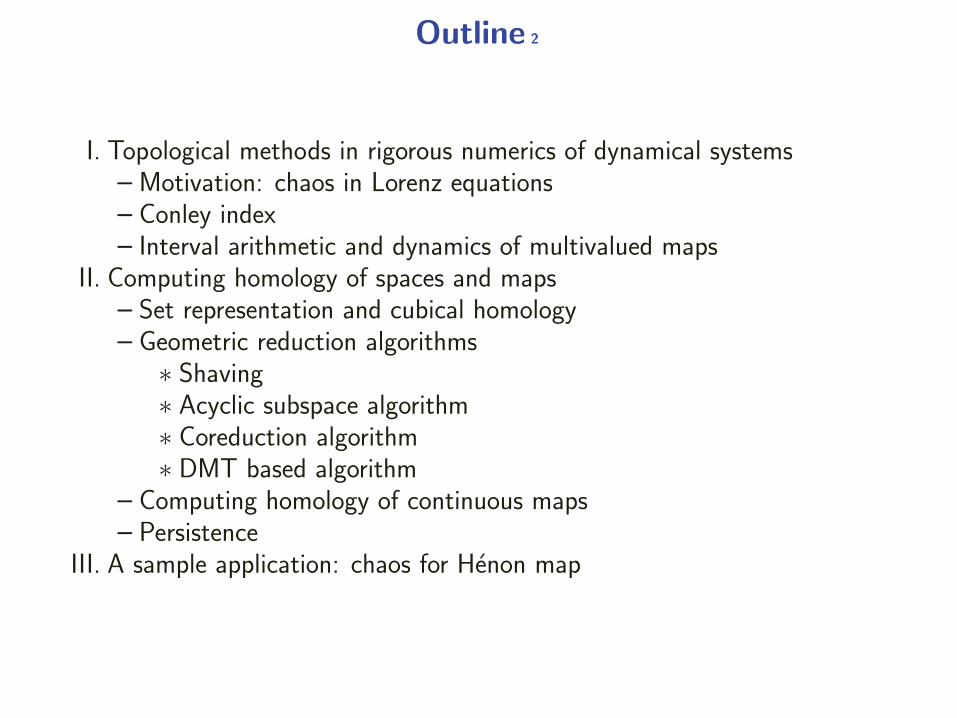
Edward Lorenz 3

Edward Lorenz 1917-2008

• during the 1950s became skep-tical of the appropriateness ofthe mathematical models usedin meteorology

• in 1963 published the famouspaper: Deterministic Nonpe-riodic Flow

• the Lorenz equations:⎧⎨⎩

x = σ(y − x)y = Rx− y − xzz = xy − bz

Ghost solutions 4

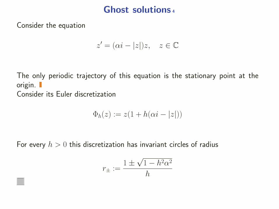
Consider the equation

z′ = (αi− |z|)z, z ∈ C

The only periodic trajectory of this equation is the stationary point at theorigin.Consider its Euler discretization

Φh(z) := z(1 + h(αi− |z|))

For every h > 0 this discretization has invariant circles of radius

r± :=1±√

1− h2α2

h

Problem 5

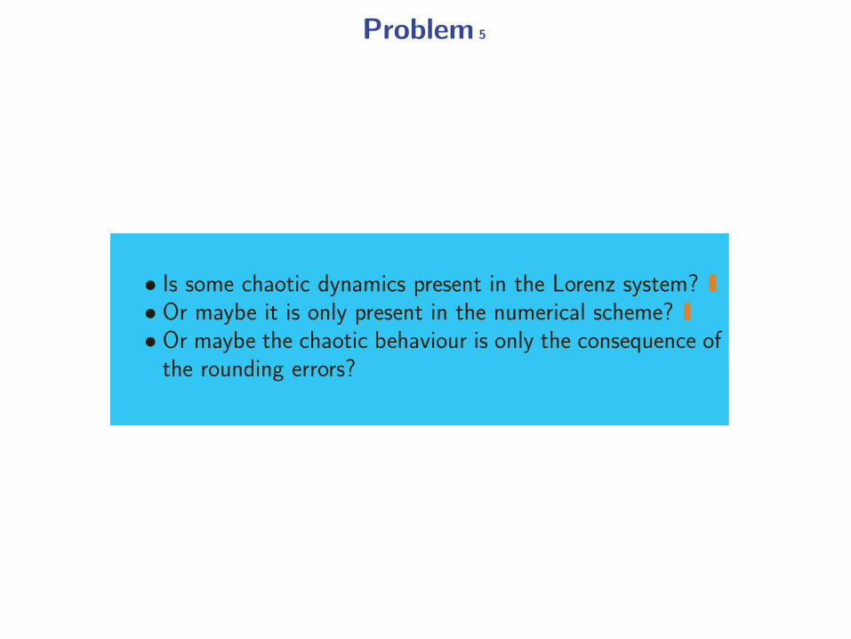
• Is some chaotic dynamics present in the Lorenz system?• Or maybe it is only present in the numerical scheme?• Or maybe the chaotic behaviour is only the consequence of

the rounding errors?

Isolated invariant sets 6

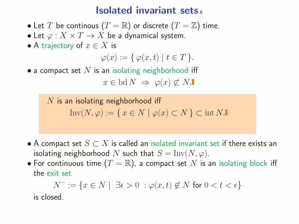
• Let T be continous (T = R) or discrete (T = Z) time.• Let ϕ : X × T → X be a dynamical system.• A trajectory of x ∈ X is

ϕ(x) := {ϕ(x, t) | t ∈ T }.• a compact set N is an isolating neighborhood iff

x ∈ bdN ⇒ ϕ(x) �⊂ N.

N is an isolating neighborhood iff

Inv(N,ϕ) := {x ∈ N | ϕ(x) ⊂ N } ⊂ intN.

• A compact set S ⊂ X is called an isolated invariant set if there exists anisolating neighborhood N such that S = Inv(N,ϕ).

• For continuous time (T = R), a compact set N is an isolating block iffthe exit set

N− := {x ∈ N | ∃ε > 0 : ϕ(x, t) �∈ N for 0 < t < ε}is closed.

Conley index 7

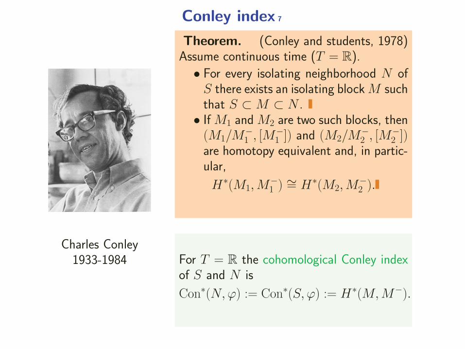
Charles Conley1933-1984

Theorem. (Conley and students, 1978)Assume continuous time (T = R).

• For every isolating neighborhood N ofS there exists an isolating block M suchthat S ⊂ M ⊂ N .

• If M1 and M2 are two such blocks, then(M1/M

−1 , [M

−1 ]) and (M2/M

−2 , [M

−2 ])

are homotopy equivalent and, in partic-ular,

H∗(M1,M−1 )

∼= H∗(M2,M−2 ).

For T = R the cohomological Conley indexof S and N is

Con∗(N,ϕ) := Con∗(S, ϕ) := H∗(M,M−).

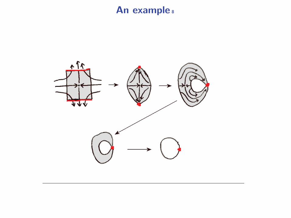
An example 8

Discrete case (T = Z) 9

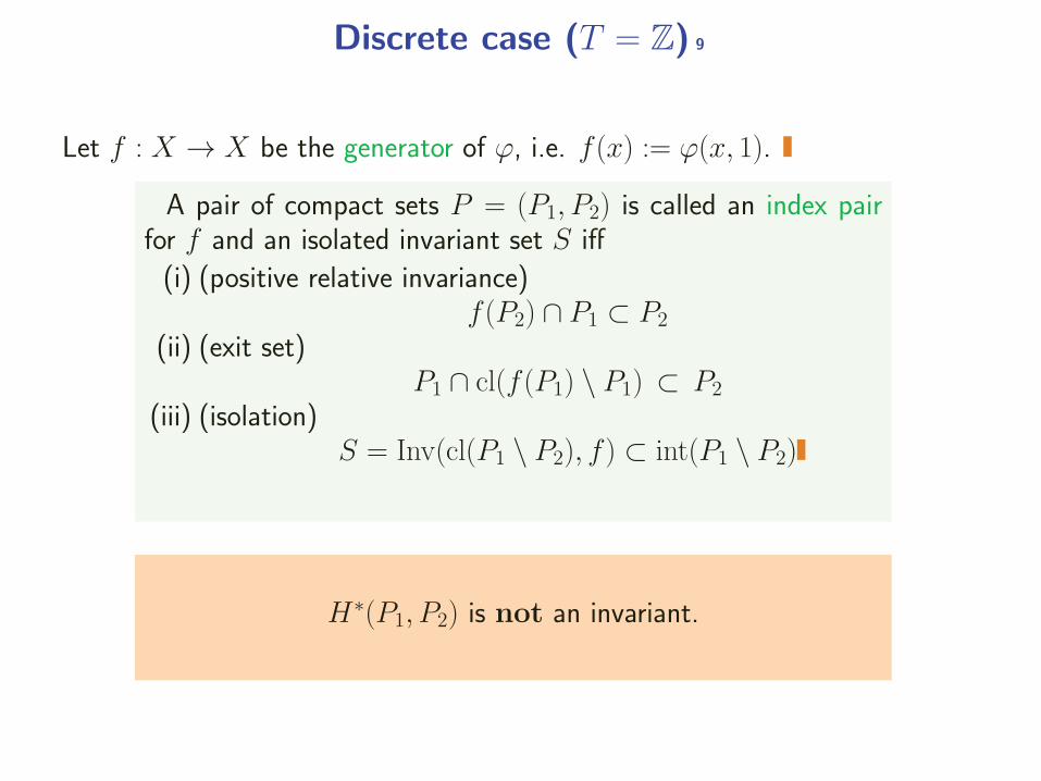
Let f : X → X be the generator of ϕ, i.e. f (x) := ϕ(x, 1).

A pair of compact sets P = (P1, P2) is called an index pairfor f and an isolated invariant set S iff

(i) (positive relative invariance)f (P2) ∩ P1 ⊂ P2

(ii) (exit set)P1 ∩ cl(f (P1) \ P1) ⊂ P2

(iii) (isolation)S = Inv(cl(P1 \ P2), f ) ⊂ int(P1 \ P2)

H∗(P1, P2) is not an invariant.

Leray Functor 10

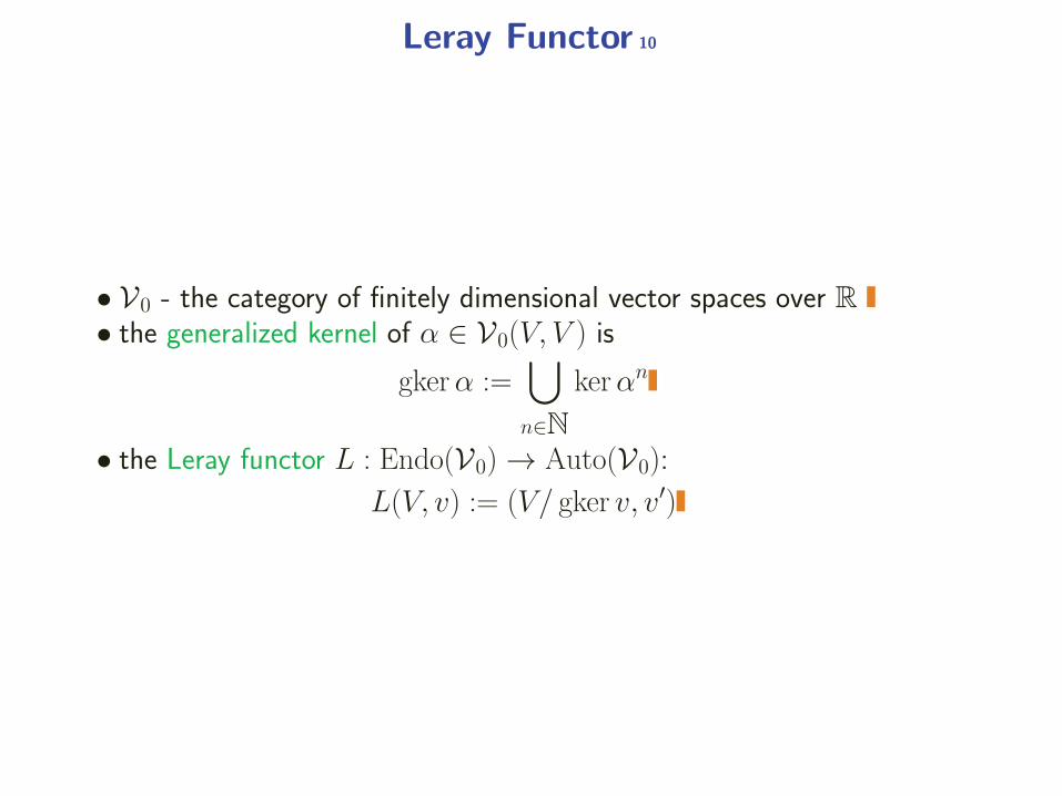
• V0 - the category of finitely dimensional vector spaces over R• the generalized kernel of α ∈ V0(V, V ) is

gkerα :=⋃n∈N

kerαn

• the Leray functor L : Endo(V0) → Auto(V0):

L(V, v) := (V/ gker v, v′)

Index quadruples and index maps 11

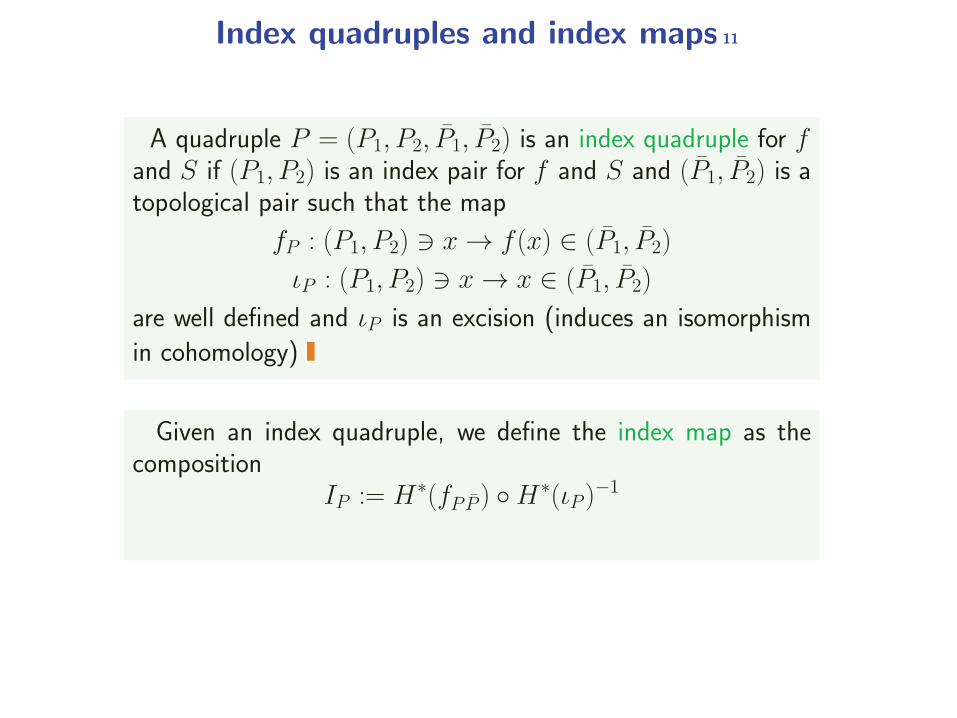
A quadruple P = (P1, P2, P1, P2) is an index quadruple for fand S if (P1, P2) is an index pair for f and S and (P1, P2) is atopological pair such that the map

fP : (P1, P2) x → f (x) ∈ (P1, P2)

ιP : (P1, P2) x → x ∈ (P1, P2)

are well defined and ιP is an excision (induces an isomorphismin cohomology)

Given an index quadruple, we define the index map as thecomposition

IP := H∗(fPP ) ◦H∗(ιP )−1

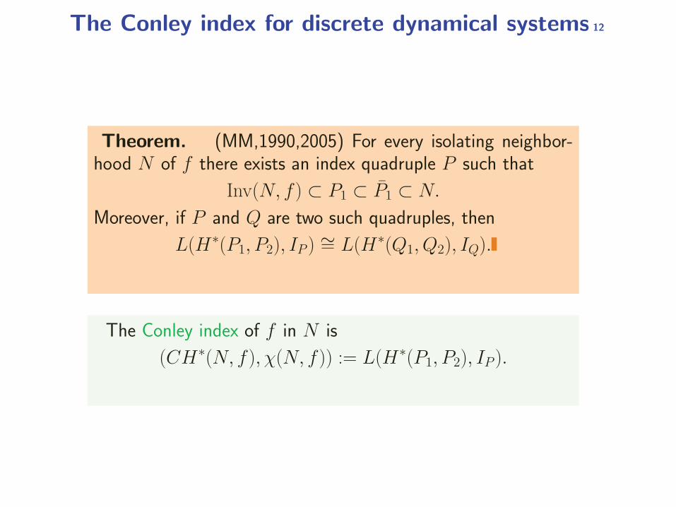
The Conley index for discrete dynamical systems 12

Theorem. (MM,1990,2005) For every isolating neighbor-hood N of f there exists an index quadruple P such that

Inv(N, f ) ⊂ P1 ⊂ P1 ⊂ N.

Moreover, if P and Q are two such quadruples, then

L(H∗(P1, P2), IP ) ∼= L(H∗(Q1, Q2), IQ).

The Conley index of f in N is

(CH∗(N, f ), χ(N, f )) := L(H∗(P1, P2), IP ).

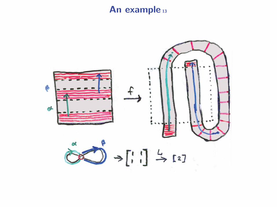
An example 13

14

It is possible to characterize the existence of chaotic dynamicsin terms of the Conley index.

15

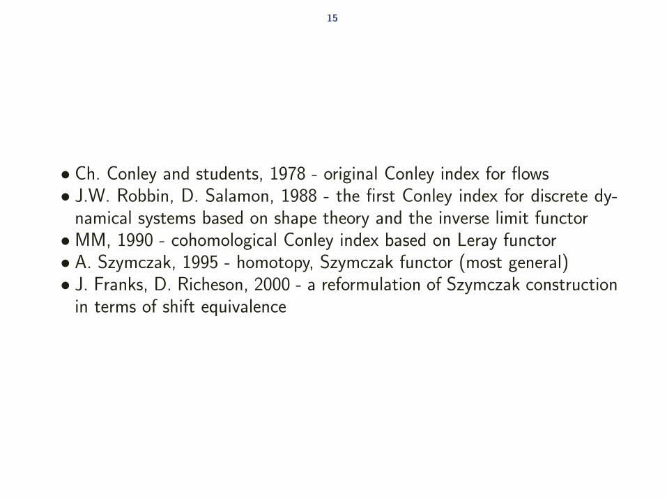
• Ch. Conley and students, 1978 - original Conley index for flows• J.W. Robbin, D. Salamon, 1988 - the first Conley index for discrete dy-

namical systems based on shape theory and the inverse limit functor• MM, 1990 - cohomological Conley index based on Leray functor• A. Szymczak, 1995 - homotopy, Szymczak functor (most general)• J. Franks, D. Richeson, 2000 - a reformulation of Szymczak construction

in terms of shift equivalence

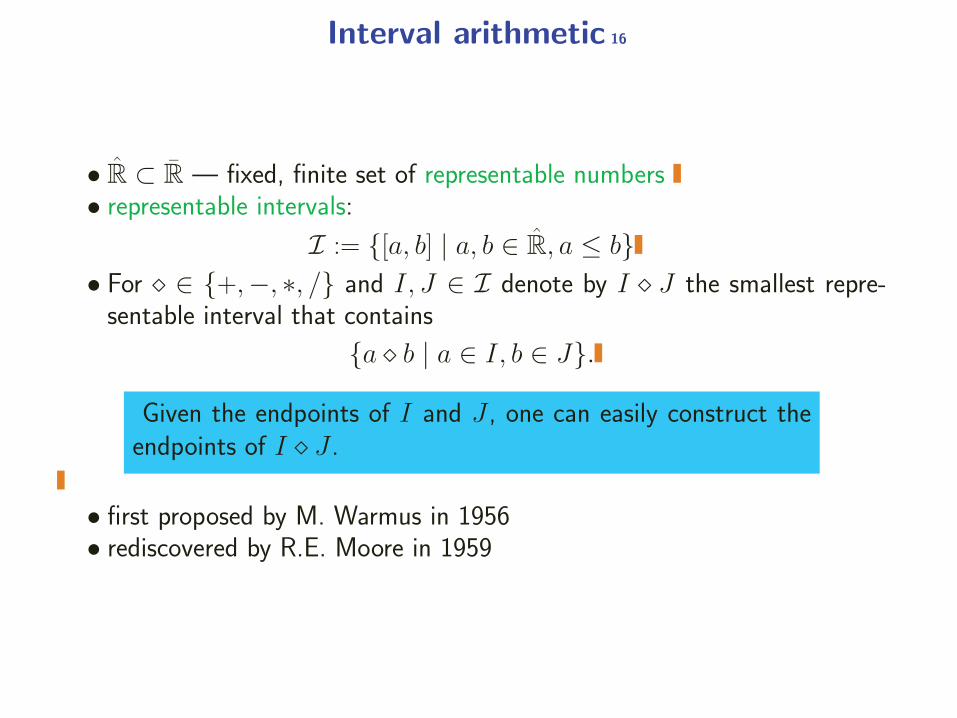
Interval arithmetic 16

• R ⊂ R — fixed, finite set of representable numbers• representable intervals:

I := {[a, b] | a, b ∈ R, a ≤ b}• For � ∈ {+,−, ∗, /} and I, J ∈ I denote by I � J the smallest repre-

sentable interval that contains

{a � b | a ∈ I, b ∈ J}.Given the endpoints of I and J , one can easily construct the

endpoints of I � J .

• first proposed by M. Warmus in 1956• rediscovered by R.E. Moore in 1959

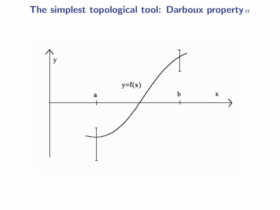
The simplest topological tool: Darboux property 17

Advanced tool: topological dynamics of multivalued maps 18

19

• Interval arithmetic combined with classical numerical meth-ods for dynamical systems provides rigorous enclosures oftrajectories of dynamical systems in the form of so calledcombinatorial multivalued representation.

• There are algorithms which use this combinatorial multival-ued representation to rigorously construct index pairs andindex quadruples of dynamical system

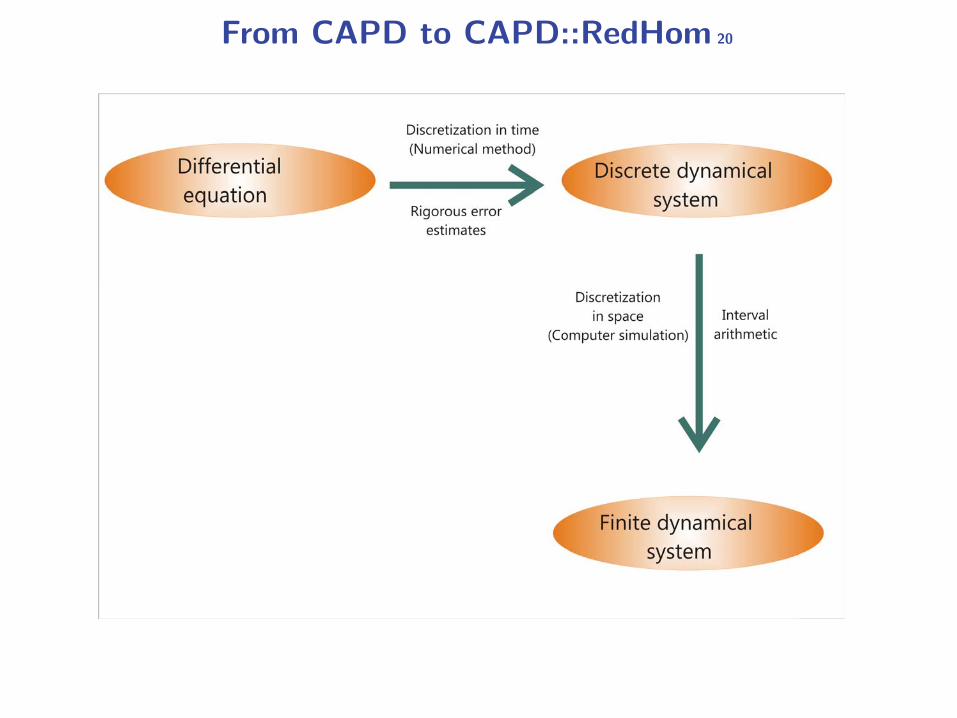
From CAPD to CAPD::RedHom 20

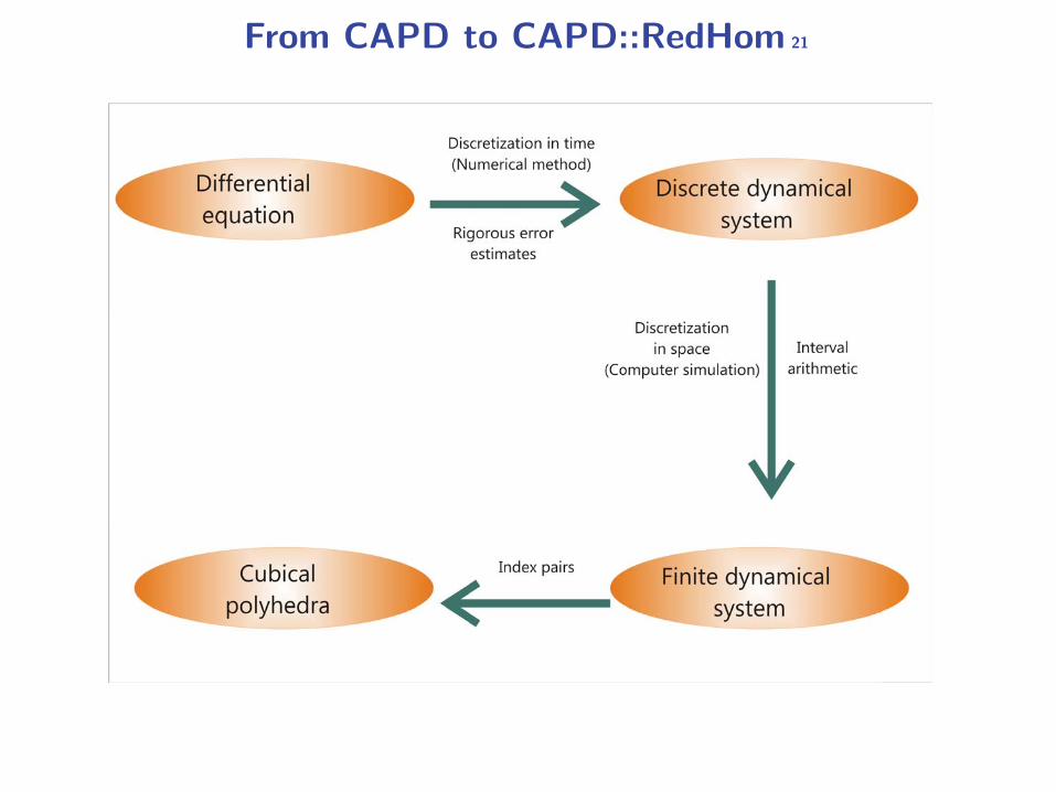
From CAPD to CAPD::RedHom 21

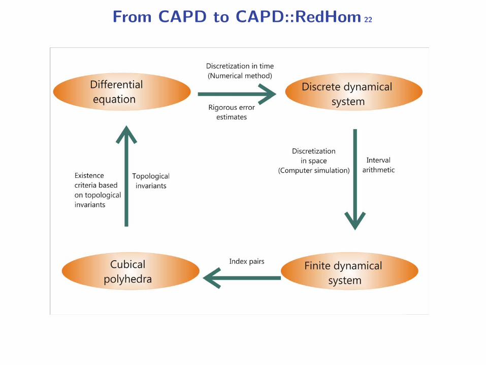
From CAPD to CAPD::RedHom 22

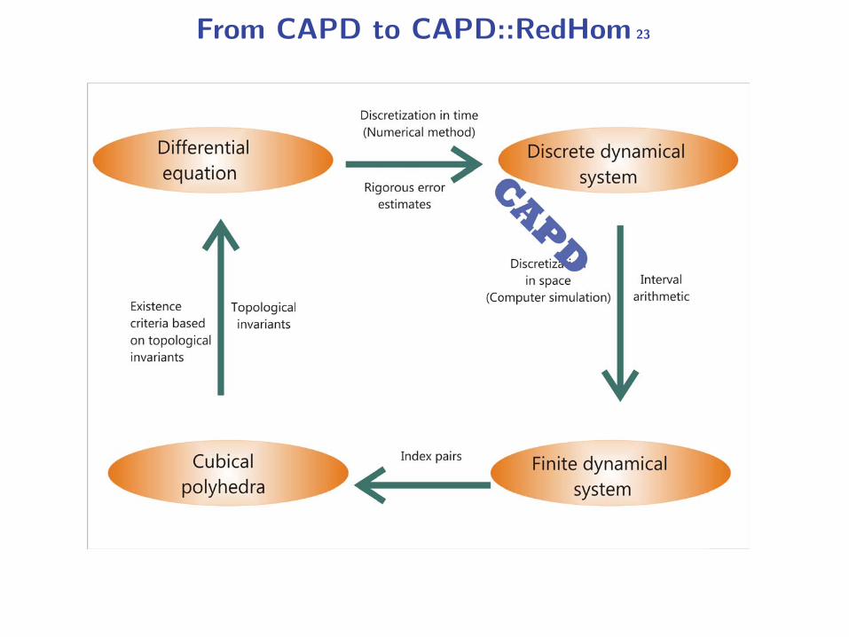
From CAPD to CAPD::RedHom 23

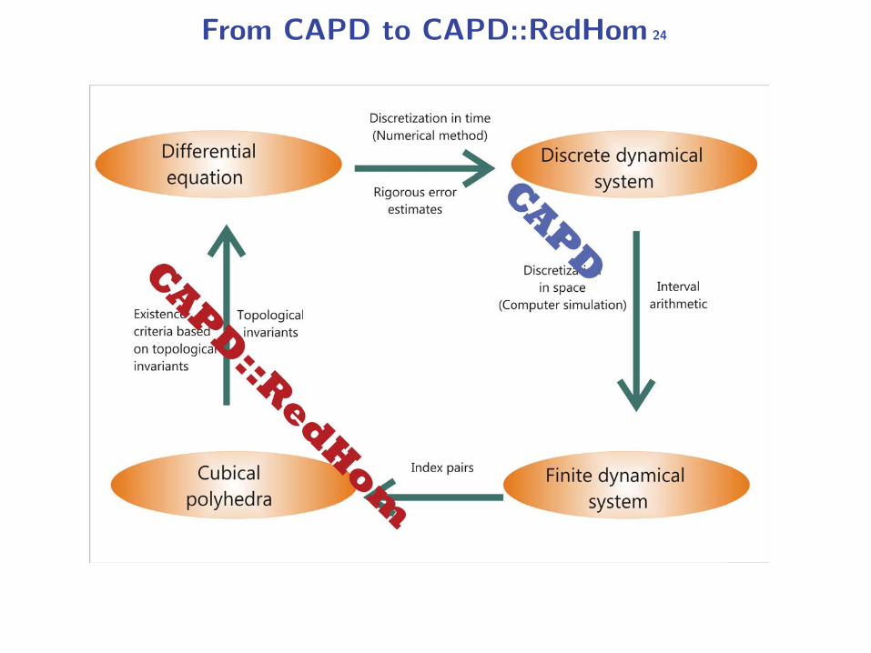
From CAPD to CAPD::RedHom 24

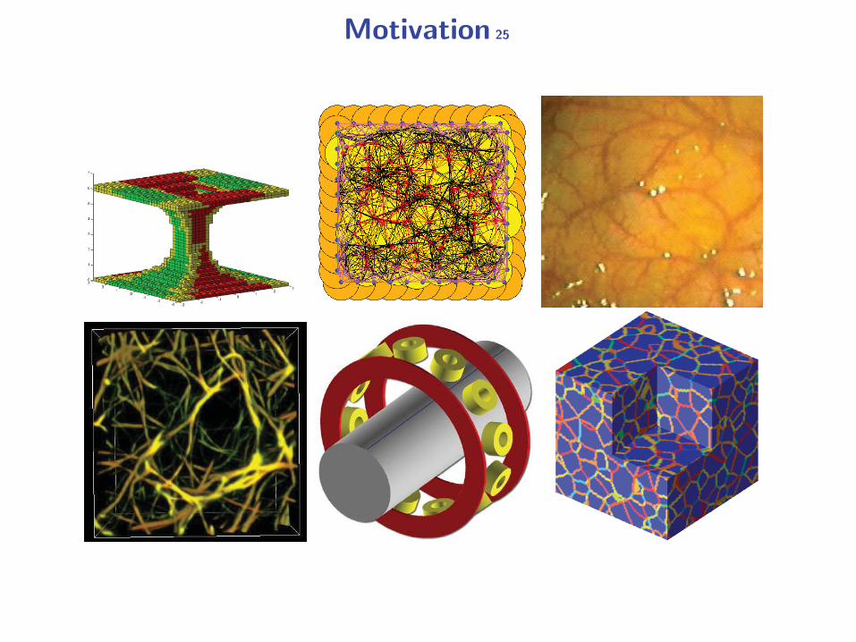
Motivation 25

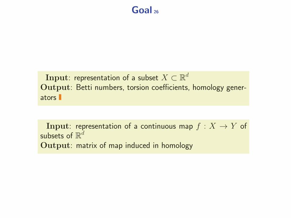
Goal 26

Input: representation of a subset X ⊂ Rd

Output: Betti numbers, torsion coefficients, homology gener-ators

Input: representation of a continuous map f : X → Y ofsubsets of Rd

Output: matrix of map induced in homology

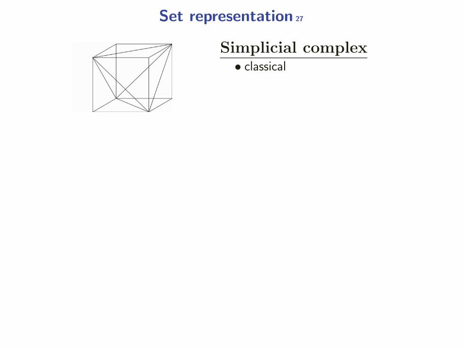
Set representation 27

Simplicial complex• classical

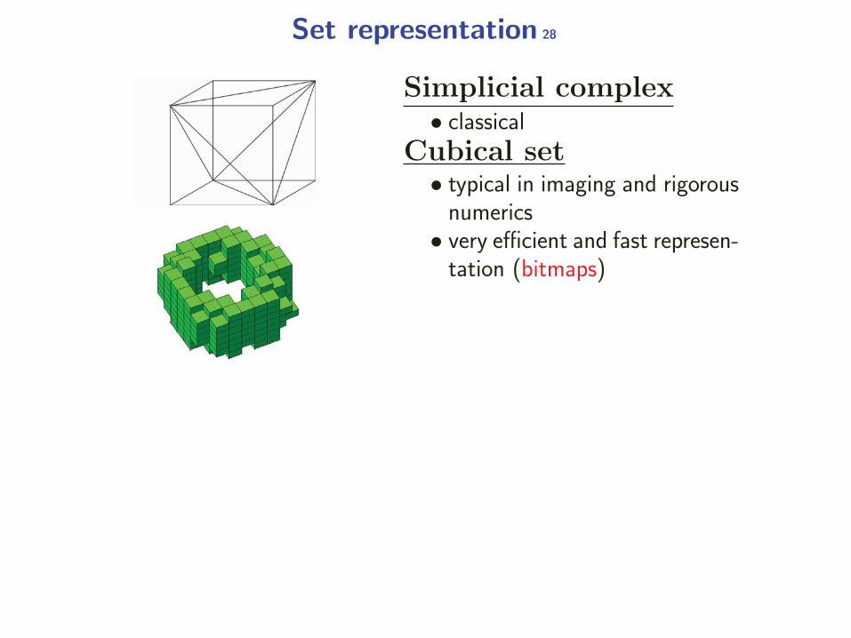
Set representation 28

Simplicial complex• classical

Cubical set• typical in imaging and rigorous

numerics• very efficient and fast represen-

tation (bitmaps)

Set representation 29

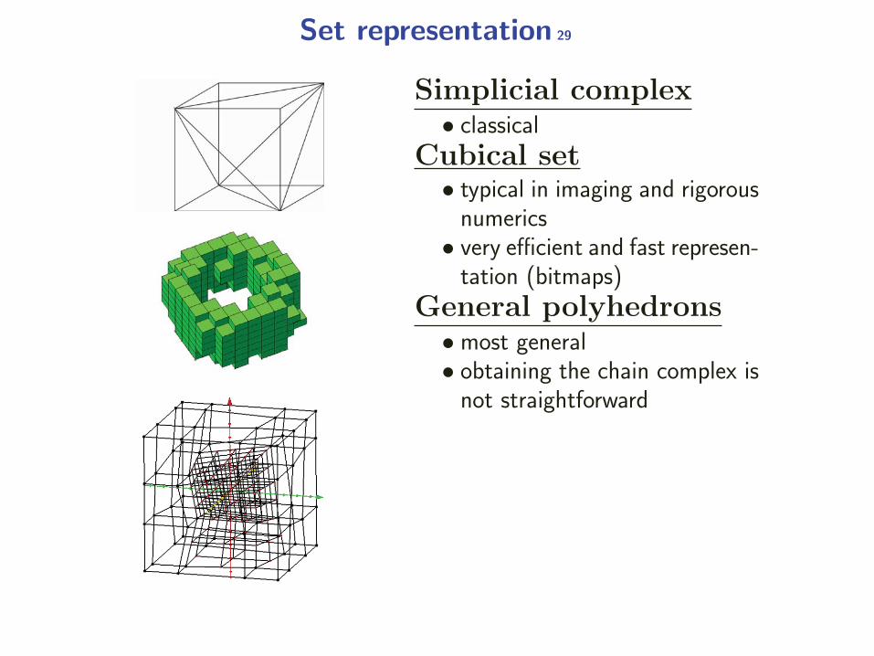
Simplicial complex• classical

Cubical set• typical in imaging and rigorous

numerics• very efficient and fast represen-

tation (bitmaps)

General polyhedrons• most general• obtaining the chain complex is

not straightforward

Input 30

Algebraists expect matrices of boundary maps as input of ho-mology computations.

• On input: a set represented as a list of top dimensionalcells (cubes, simplices, ...)

• Generation of faces, incidence coefficients and boundarymaps, whenever necessary, must be considered a part ofthe job!

Cubical sets 31

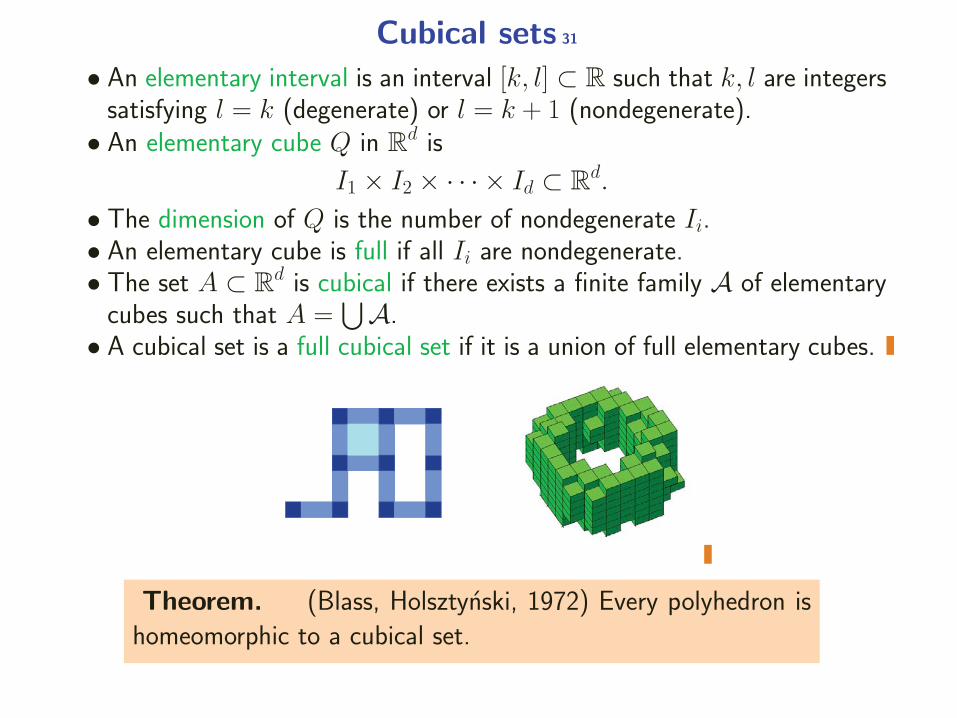
• An elementary interval is an interval [k, l] ⊂ R such that k, l are integerssatisfying l = k (degenerate) or l = k + 1 (nondegenerate).

• An elementary cube Q in Rd is

I1 × I2 × · · · × Id ⊂ Rd.

• The dimension of Q is the number of nondegenerate Ii.• An elementary cube is full if all Ii are nondegenerate.• The set A ⊂ R

d is cubical if there exists a finite family A of elementarycubes such that A =

⋃A.• A cubical set is a full cubical set if it is a union of full elementary cubes.

Theorem. (Blass, Holsztynski, 1972) Every polyhedron ishomeomorphic to a cubical set.

Cubical Chains 32

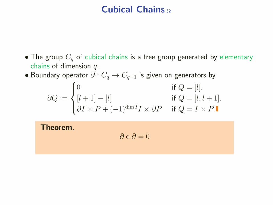
• The group Cq of cubical chains is a free group generated by elementarychains of dimension q.

• Boundary operator ∂ : Cq → Cq−1 is given on generators by

∂Q :=

⎧⎪⎨⎪⎩0 if Q = [l],

[l + 1]− [l] if Q = [l, l + 1].

∂I × P + (−1)dim II × ∂P if Q = I × P .

Theorem.∂ ◦ ∂ = 0

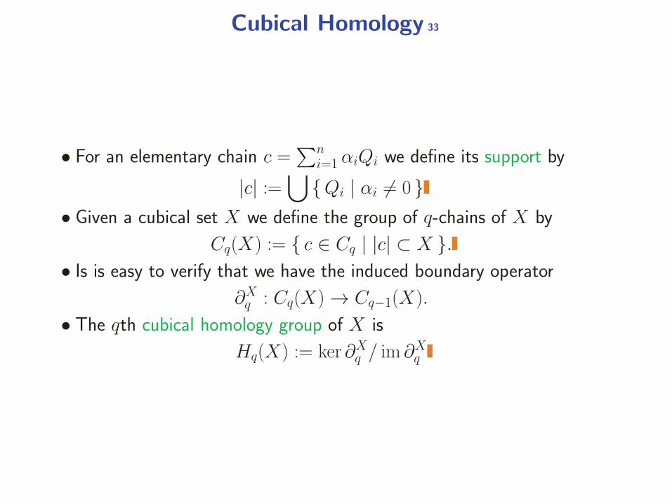
Cubical Homology 33

• For an elementary chain c =∑n

i=1 αiQi we define its support by

|c| :=⋃

{Qi | αi �= 0 }• Given a cubical set X we define the group of q-chains of X by

Cq(X) := { c ∈ Cq | |c| ⊂ X }.• Is is easy to verify that we have the induced boundary operator

∂Xq : Cq(X) → Cq−1(X).

• The qth cubical homology group of X is

Hq(X) := ker ∂Xq / im ∂X

q

Standard approach 34

Immediate algebraization:

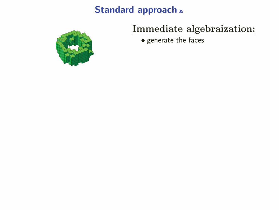
Standard approach 35

Immediate algebraization:• generate the faces

Standard approach 36

Dk =

⎡⎢⎢⎢⎢⎣

1 −1 0 0 ...1 0 1 0 ...−1 1 0 0 ...

0 1 0 0 .... . . . .

⎤⎥⎥⎥⎥⎦

Immediate algebraization:• generate the faces• construct the boundary maps

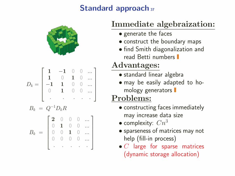
Standard approach 37

Dk =

⎡⎢⎢⎢⎢⎣

1 −1 0 0 ...1 0 1 0 ...−1 1 0 0 ...

0 1 0 0 .... . . . .

⎤⎥⎥⎥⎥⎦

Bk = Q−1DkR

Bk =

⎡⎢⎢⎢⎢⎣

2 0 0 0 ...0 1 0 0 ...0 0 1 0 ...0 0 0 0 .... . . . .

⎤⎥⎥⎥⎥⎦

Immediate algebraization:• generate the faces• construct the boundary maps• find Smith diagonalization and

read Betti numbers

Advantages:• standard linear algebra• may be easily adapted to ho-

mology generators

Problems:• constructing faces immediately

may increase data size• complexity: Cn3

• sparseness of matrices may nothelp (fill-in process)

• C large for sparse matrices(dynamic storage allocation)

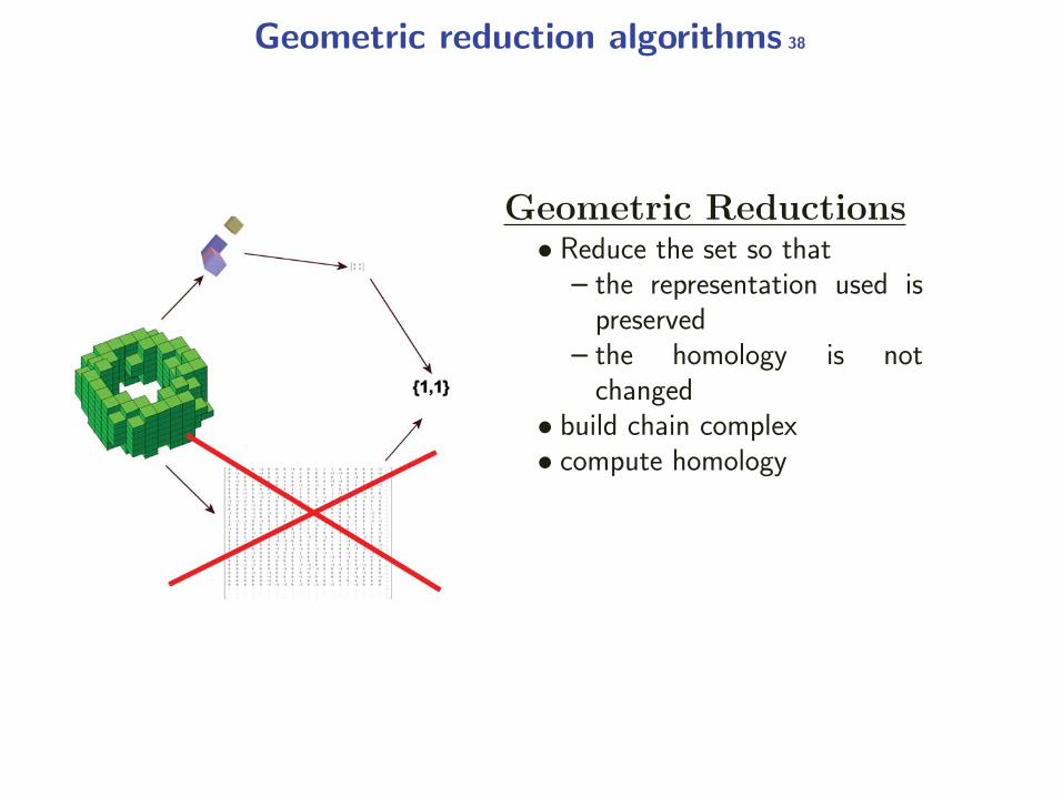
Geometric reduction algorithms 38

Geometric Reductions• Reduce the set so that

– the representation used ispreserved

– the homology is notchanged

• build chain complex• compute homology

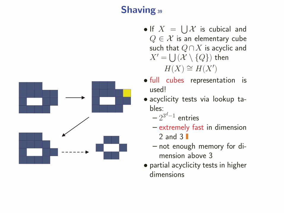
Shaving 39

• If X =⋃X is cubical and

Q ∈ X is an elementary cubesuch that Q∩X is acyclic andX ′ =

⋃(X \ {Q}) then

H(X) ∼= H(X ′)• full cubes representation is

used!• acyclicity tests via lookup ta-

bles:– 23

d−1 entries– extremely fast in dimension

2 and 3– not enough memory for di-

mension above 3• partial acyclicity tests in higher

dimensions

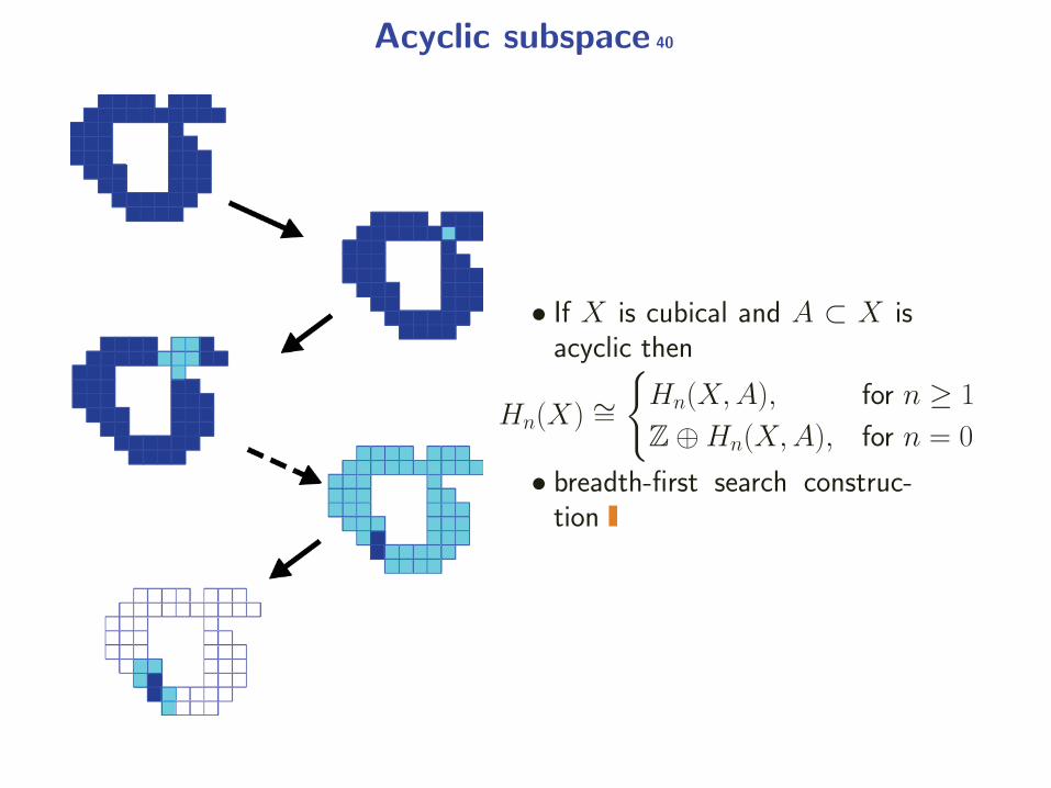
Acyclic subspace 40

• If X is cubical and A ⊂ X isacyclic then

Hn(X) ∼={Hn(X,A), for n ≥ 1

Z⊕Hn(X,A), for n = 0

• breadth-first search construc-tion

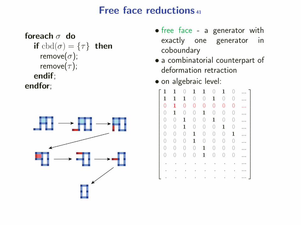
Free face reductions 41

foreach σ doif cbd(σ) = {τ} then

remove(σ);remove(τ );

endif;endfor;

• free face - a generator withexactly one generator incoboundary

• a combinatorial counterpart ofdeformation retraction

• on algebraic level:⎡⎢⎢⎢⎢⎢⎢⎢⎢⎢⎢⎢⎢⎢⎢⎢⎢⎢⎢⎢⎣

1 1 0 1 1 0 1 0 ...1 1 1 0 0 1 0 0 ...0 1 0 0 0 0 0 0 ...0 1 0 0 1 0 0 0 ...0 0 1 0 0 1 0 0 ...0 0 1 0 0 0 1 0 ...0 0 0 1 0 0 0 1 ...0 0 0 1 0 0 0 0 ...0 0 0 0 1 0 0 0 ...0 0 0 0 1 0 0 0 .... . . . . . . . .... . . . . . . . .... . . . . . . . ...

⎤⎥⎥⎥⎥⎥⎥⎥⎥⎥⎥⎥⎥⎥⎥⎥⎥⎥⎥⎥⎦

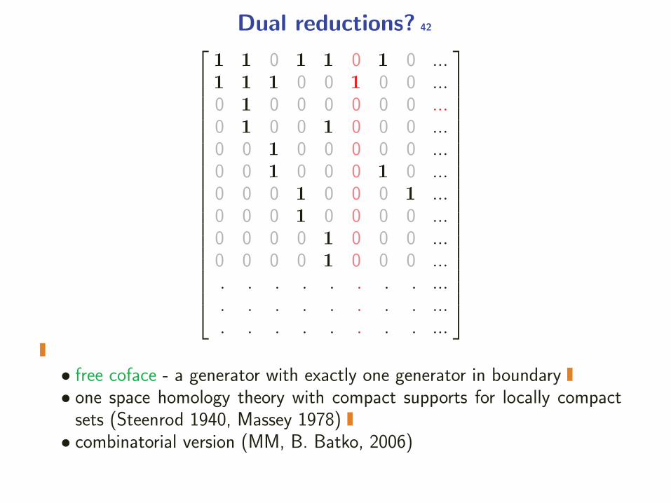
Dual reductions? 42⎡⎢⎢⎢⎢⎢⎢⎢⎢⎢⎢⎢⎢⎢⎢⎢⎢⎢⎢⎢⎣

1 1 0 1 1 0 1 0 ...1 1 1 0 0 1 0 0 ...0 1 0 0 0 0 0 0 ...0 1 0 0 1 0 0 0 ...0 0 1 0 0 0 0 0 ...0 0 1 0 0 0 1 0 ...0 0 0 1 0 0 0 1 ...0 0 0 1 0 0 0 0 ...0 0 0 0 1 0 0 0 ...0 0 0 0 1 0 0 0 .... . . . . . . . .... . . . . . . . .... . . . . . . . ...

⎤⎥⎥⎥⎥⎥⎥⎥⎥⎥⎥⎥⎥⎥⎥⎥⎥⎥⎥⎥⎦

• free coface - a generator with exactly one generator in boundary• one space homology theory with compact supports for locally compact

sets (Steenrod 1940, Massey 1978)• combinatorial version (MM, B. Batko, 2006)

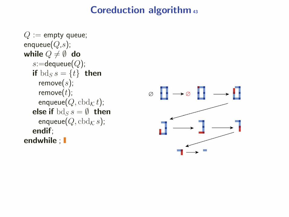
Coreduction algorithm 43

Q := empty queue;enqueue(Q,s);while Q �= ∅ do

s:=dequeue(Q);if bdS s = {t} then

remove(s);remove(t);enqueue(Q, cbdK t);

else if bdS s = ∅ thenenqueue(Q, cbdK s);

endif;endwhile ;

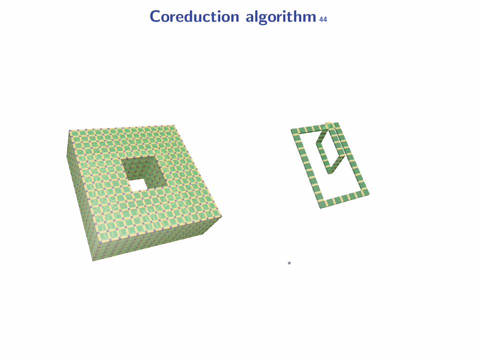
Coreduction algorithm 44

Coreductions for S-complexes 45

• S-complex - a free chain complex with a fixed basis S which allowscomputation of incidence coefficients κ(s, t) directly from the coding ofthe basis

• Examples: cubical complexes, simplicial complexes• Rectangular CW-complexes (P. D�lotko, T. Kaczynski, MM, T. Wanner,

2010)

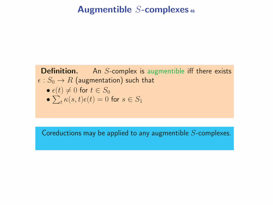
Augmentible S-complexes 46

Definition. An S-complex is augmentible iff there existsε : S0 → R (augmentation) such that

• ε(t) �= 0 for t ∈ S0

•∑t κ(s, t)ε(t) = 0 for s ∈ S1

Coreductions may be applied to any augmentible S-complexes.

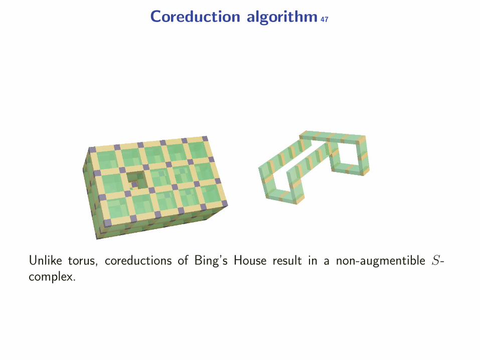
Coreduction algorithm 47

Unlike torus, coreductions of Bing’s House result in a non-augmentible S-complex.

Morse-Forman theory 48

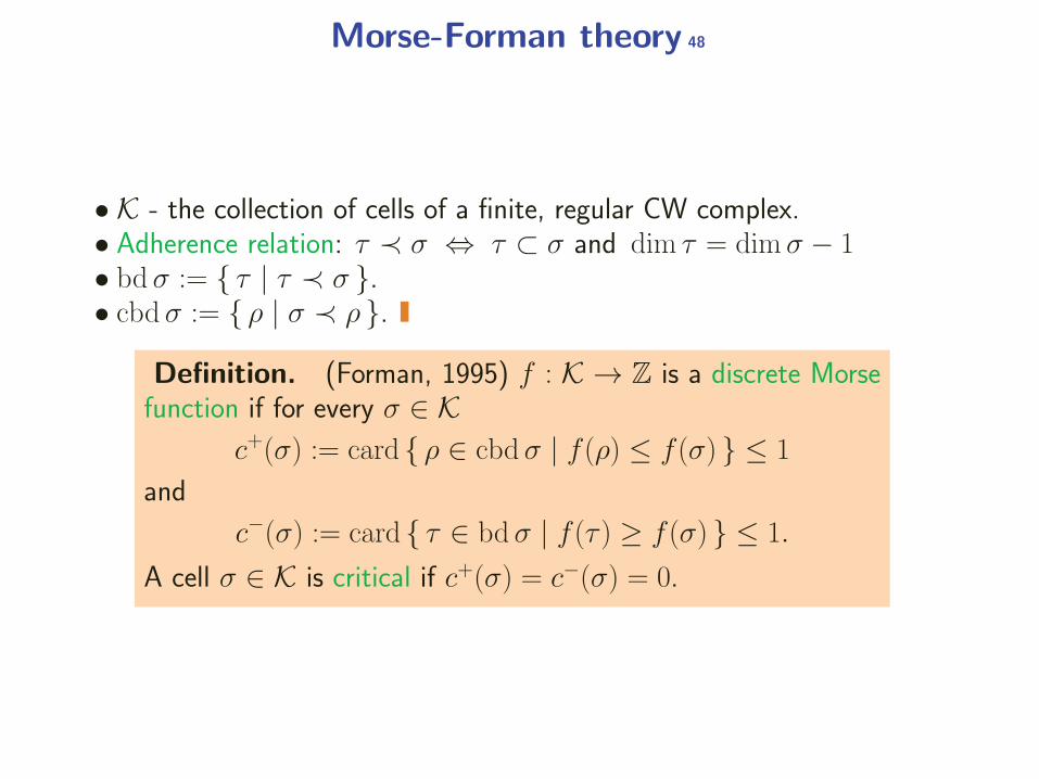
• K - the collection of cells of a finite, regular CW complex.• Adherence relation: τ ≺ σ ⇔ τ ⊂ σ and dim τ = dimσ − 1• bd σ := { τ | τ ≺ σ }.• cbd σ := { ρ | σ ≺ ρ }.

Definition. (Forman, 1995) f : K → Z is a discrete Morsefunction if for every σ ∈ K

c+(σ) := card { ρ ∈ cbd σ | f (ρ) ≤ f (σ) } ≤ 1

and

c−(σ) := card { τ ∈ bd σ | f (τ ) ≥ f (σ) } ≤ 1.

A cell σ ∈ K is critical if c+(σ) = c−(σ) = 0.

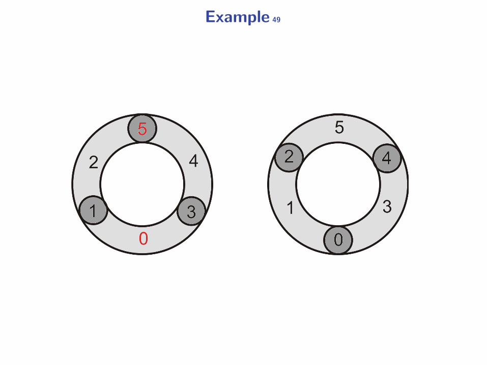
Example 49

Morse-Froman Homology 50

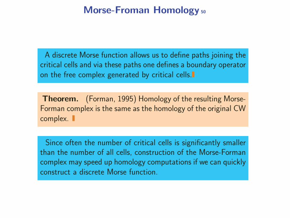
A discrete Morse function allows us to define paths joining thecritical cells and via these paths one defines a boundary operatoron the free complex generated by critical cells.

Theorem. (Forman, 1995) Homology of the resulting Morse-Forman complex is the same as the homology of the original CWcomplex.

Since often the number of critical cells is significantly smallerthan the number of all cells, construction of the Morse-Formancomplex may speed up homology computations if we can quicklyconstruct a discrete Morse function.

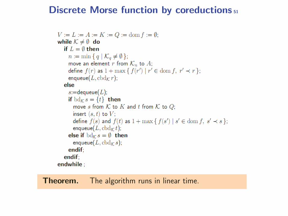
Discrete Morse function by coreductions 51

Theorem. The algorithm runs in linear time.

CAPD::RedHom 52

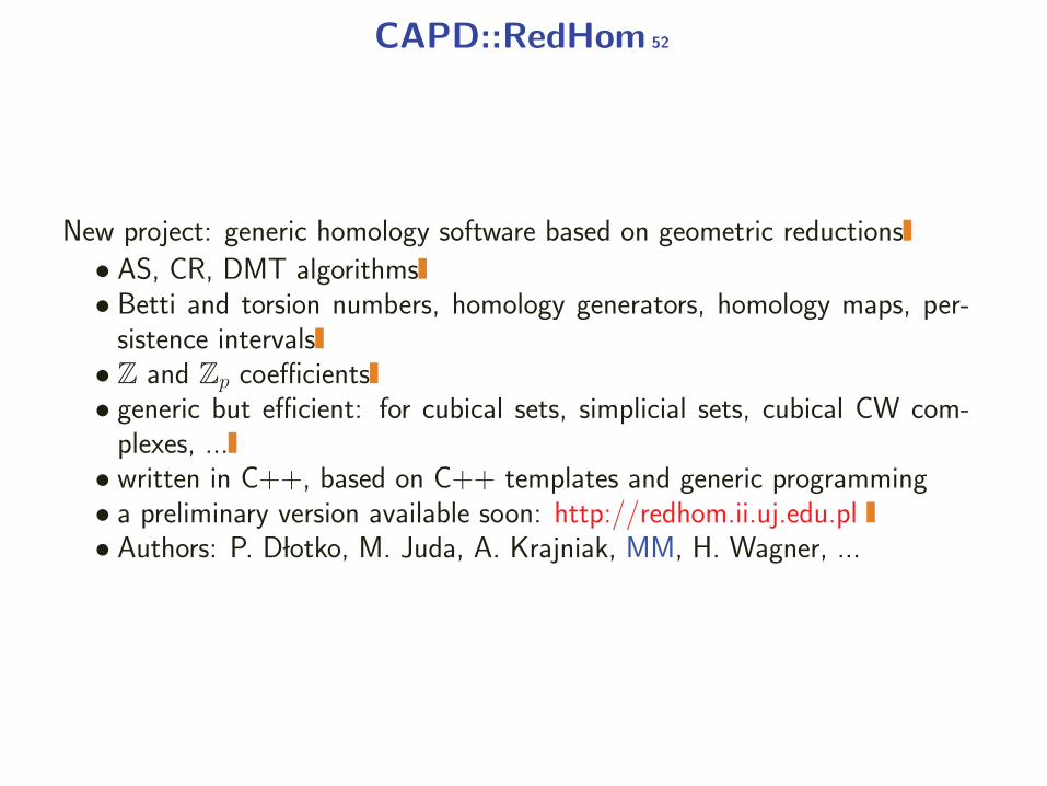
New project: generic homology software based on geometric reductions

• AS, CR, DMT algorithms• Betti and torsion numbers, homology generators, homology maps, per-

sistence intervals• Z and Zp coefficients• generic but efficient: for cubical sets, simplicial sets, cubical CW com-

plexes, ...• written in C++, based on C++ templates and generic programming• a preliminary version available soon: http://redhom.ii.uj.edu.pl• Authors: P. D�lotko, M. Juda, A. Krajniak, MM, H. Wagner, ...

Numerical examples - manifolds 53

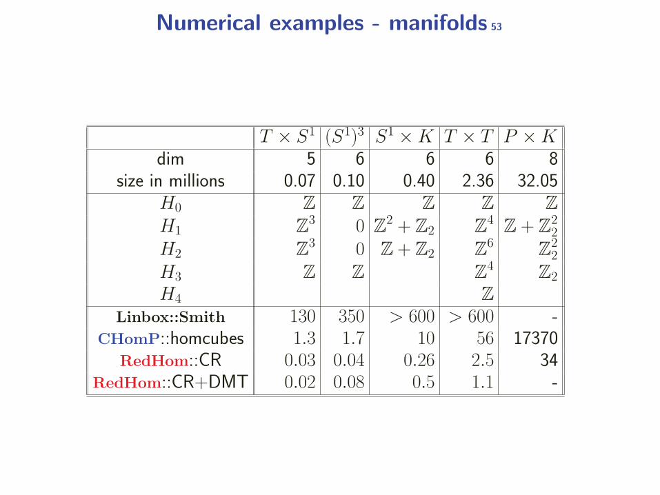
T × S1 (S1)3 S1 ×K T × T P ×Kdim 5 6 6 6 8

size in millions 0.07 0.10 0.40 2.36 32.05H0 Z Z Z Z Z

H1 Z3 0 Z

2 + Z2 Z4Z + Z

22

H2 Z3 0 Z + Z2 Z

6Z22

H3 Z Z Z4

Z2

H4 Z

Linbox::Smith 130 350 > 600 > 600 -CHomP::homcubes 1.3 1.7 10 56 17370

RedHom::CR 0.03 0.04 0.26 2.5 34RedHom::CR+DMT 0.02 0.08 0.5 1.1 -

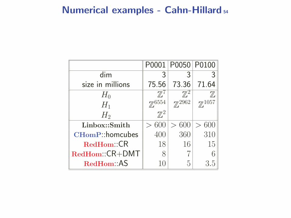
Numerical examples - Cahn-Hillard 54

P0001 P0050 P0100dim 3 3 3

size in millions 75.56 73.36 71.64H0 Z

7Z2

Z

H1 Z6554

Z2962

Z1057

H2 Z2

Linbox::Smith > 600 > 600 > 600CHomP::homcubes 400 360 310

RedHom::CR 18 16 15RedHom::CR+DMT 8 7 6

RedHom::AS 10 5 3.5

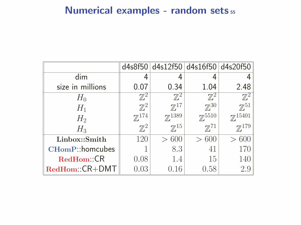
Numerical examples - random sets 55

d4s8f50 d4s12f50 d4s16f50 d4s20f50dim 4 4 4 4

size in millions 0.07 0.34 1.04 2.48H0 Z

2Z2

Z2

Z2

H1 Z2

Z17

Z30

Z51

H2 Z174

Z1389

Z5510

Z15401

H3 Z2

Z15

Z71

Z179

Linbox::Smith 120 > 600 > 600 > 600CHomP::homcubes 1 8.3 41 170

RedHom::CR 0.08 1.4 15 140RedHom::CR+DMT 0.03 0.16 0.58 2.9

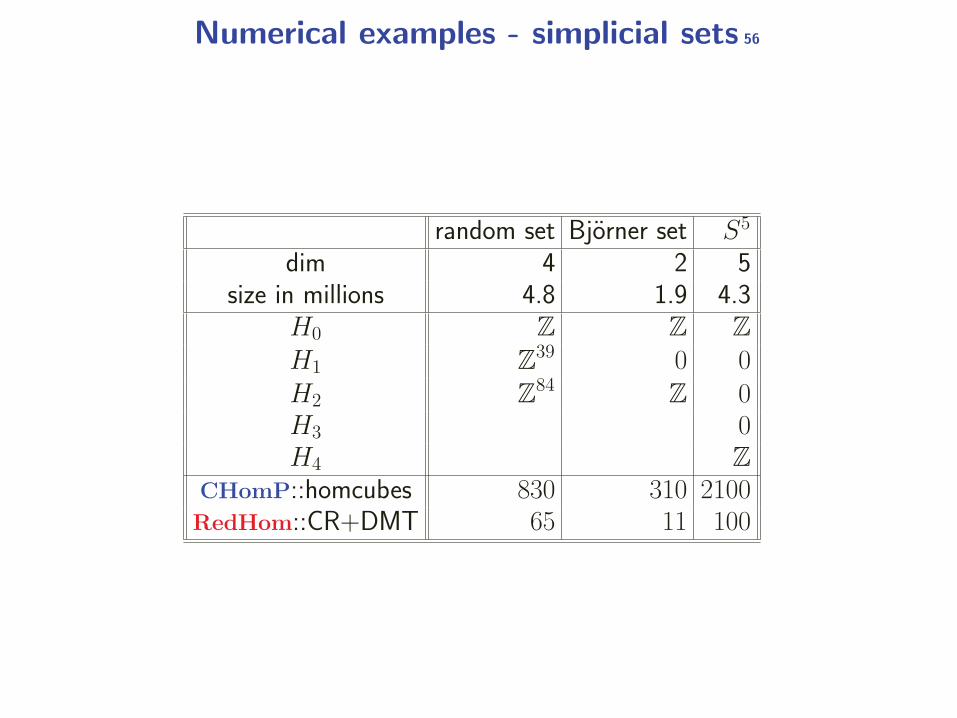
Numerical examples - simplicial sets 56

random set Bjorner set S5

dim 4 2 5size in millions 4.8 1.9 4.3

H0 Z Z Z

H1 Z39 0 0

H2 Z84

Z 0H3 0H4 Z

CHomP::homcubes 830 310 2100RedHom::CR+DMT 65 11 100

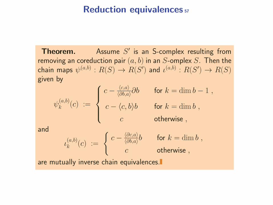
Reduction equivalences 57

Theorem. Assume S ′ is an S-complex resulting fromremoving an coreduction pair (a, b) in an S-omplex S. Then thechain maps ψ(a,b) : R(S) → R(S ′) and ι(a,b) : R(S ′) → R(S)given by

ψ(a,b)k (c) :=

⎧⎪⎪⎨⎪⎪⎩

c− 〈c,a〉〈∂b,a〉∂b for k = dim b− 1 ,

c− 〈c, b〉b for k = dim b ,

c otherwise ,

and

ι(a,b)k (c) :=

{c− 〈∂c,a〉

〈∂b,a〉b for k = dim b ,

c otherwise ,

are mutually inverse chain equivalences.

Homology model 58

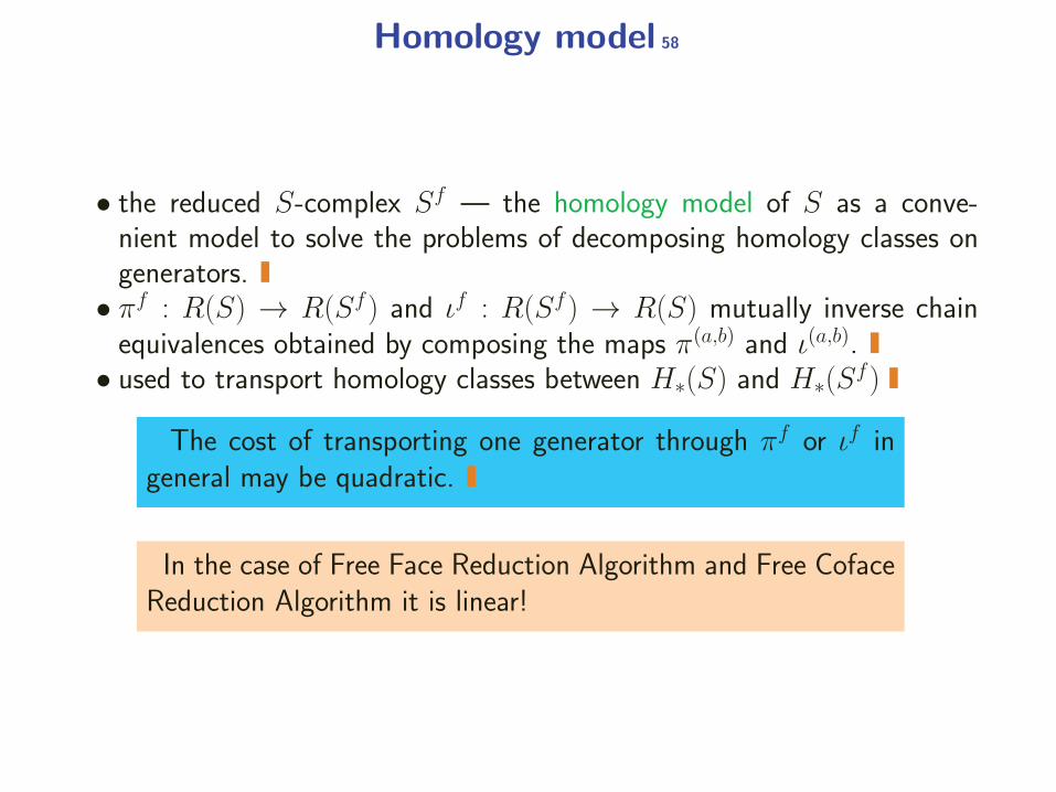
• the reduced S-complex Sf — the homology model of S as a conve-nient model to solve the problems of decomposing homology classes ongenerators.

• πf : R(S) → R(Sf) and ιf : R(Sf) → R(S) mutually inverse chainequivalences obtained by composing the maps π(a,b) and ι(a,b).

• used to transport homology classes between H∗(S) and H∗(Sf)

The cost of transporting one generator through πf or ιf ingeneral may be quadratic.

In the case of Free Face Reduction Algorithm and Free CofaceReduction Algorithm it is linear!

Homology generators 59

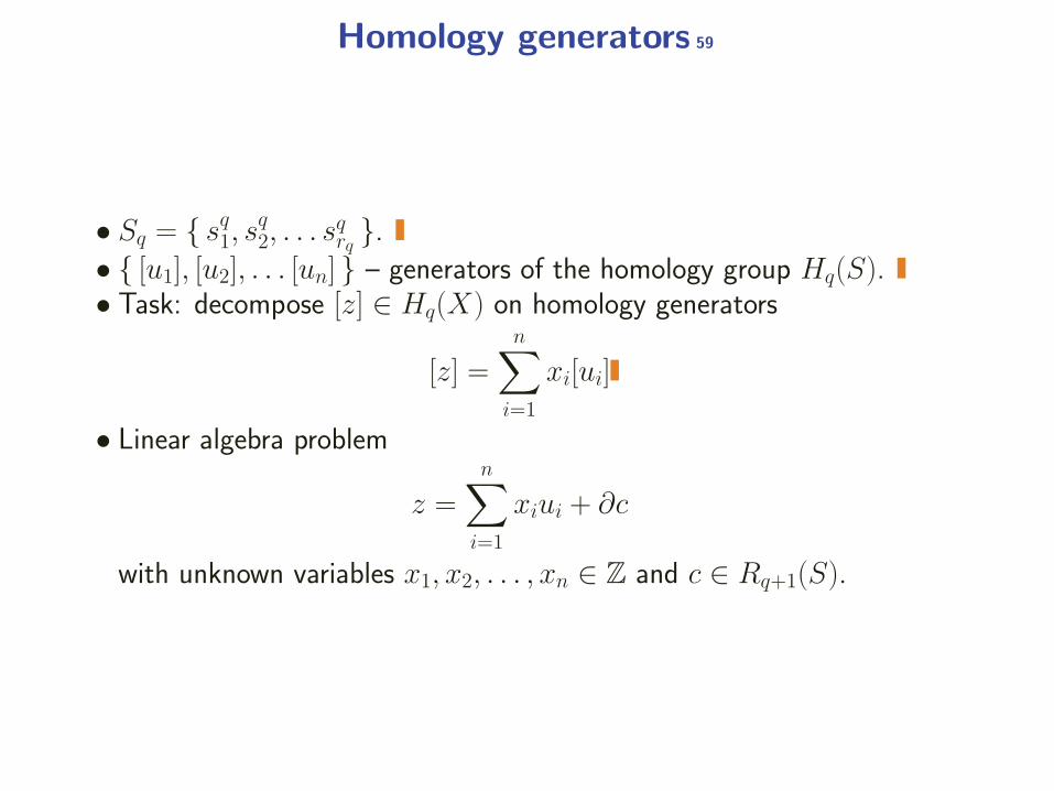
• Sq = { sq1, sq2, . . . sqrq }.

• { [u1], [u2], . . . [un] } – generators of the homology group Hq(S).• Task: decompose [z] ∈ Hq(X) on homology generators

[z] =n∑

i=1

xi[ui]

• Linear algebra problem

z =

n∑i=1

xiui + ∂c

with unknown variables x1, x2, . . . , xn ∈ Z and c ∈ Rq+1(S).

Homology generators 60

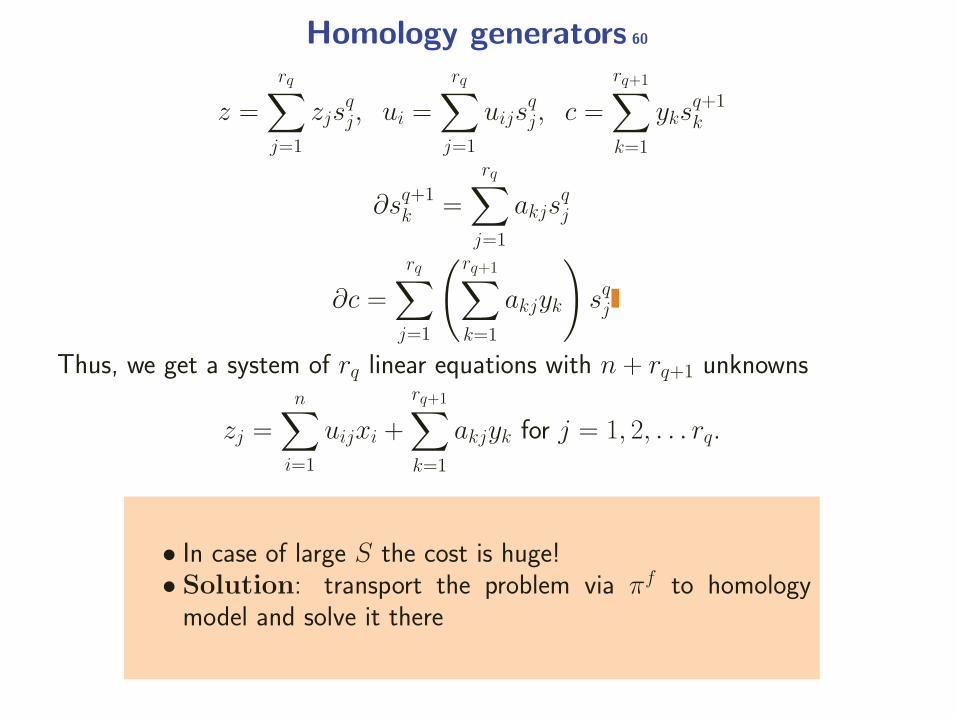
z =

rq∑j=1

zjsqj, ui =

rq∑j=1

uijsqj, c =

rq+1∑k=1

yksq+1k

∂sq+1k =

rq∑j=1

akjsqj

∂c =

rq∑j=1

(rq+1∑k=1

akjyk

)sqj

Thus, we get a system of rq linear equations with n + rq+1 unknowns

zj =

n∑i=1

uijxi +

rq+1∑k=1

akjyk for j = 1, 2, . . . rq.

• In case of large S the cost is huge!• Solution: transport the problem via πf to homology

model and solve it there

Homology of cubical maps 61

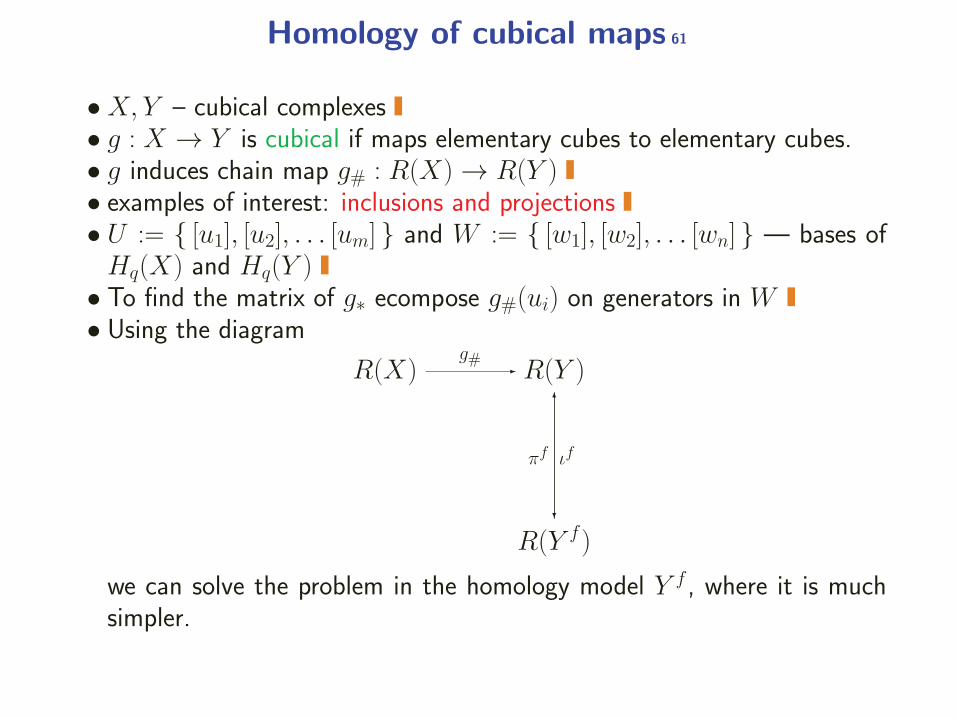
•X, Y – cubical complexes• g : X → Y is cubical if maps elementary cubes to elementary cubes.• g induces chain map g# : R(X) → R(Y )• examples of interest: inclusions and projections• U := { [u1], [u2], . . . [um] } and W := { [w1], [w2], . . . [wn] } — bases ofHq(X) and Hq(Y )

• To find the matrix of g∗ ecompose g#(ui) on generators in W• Using the diagram

R(X) R(Y )

R(Y f)

�g#

�

πf

�

ιf

we can solve the problem in the homology model Y f , where it is muchsimpler.

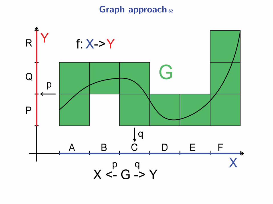
Graph approach 62

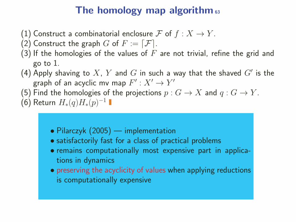
The homology map algorithm 63

(1) Construct a combinatorial enclosure F of f : X → Y .(2) Construct the graph G of F := �F�.(3) If the homologies of the values of F are not trivial, refine the grid and

go to 1.(4) Apply shaving to X , Y and G in such a way that the shaved G′ is the

graph of an acyclic mv map F ′ : X ′ → Y ′

(5) Find the homologies of the projections p : G → X and q : G → Y .(6) Return H∗(q)H∗(p)−1

• Pilarczyk (2005) — implementation• satisfactorily fast for a class of practical problems• remains computationally most expensive part in applica-

tions in dynamics• preserving the acyclicity of values when applying reductions

is computationally expensive

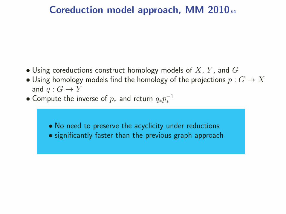
Coreduction model approach, MM 2010 64

• Using coreductions construct homology models of X , Y , and G• Using homology models find the homology of the projections p : G → X

and q : G → Y• Compute the inverse of p∗ and return q∗p−1

∗

• No need to preserve the acyclicity under reductions• significantly faster than the previous graph approach

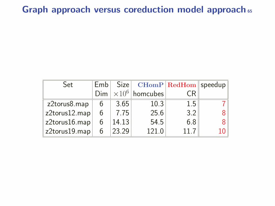
Graph approach versus coreduction model approach 65

Set Emb Size CHomP RedHom speedupDim ×106 homcubes CR

z2torus8.map 6 3.65 10.3 1.5 7z2torus12.map 6 7.75 25.6 3.2 8z2torus16.map 6 14.13 54.5 6.8 8z2torus19.map 6 23.29 121.0 11.7 10

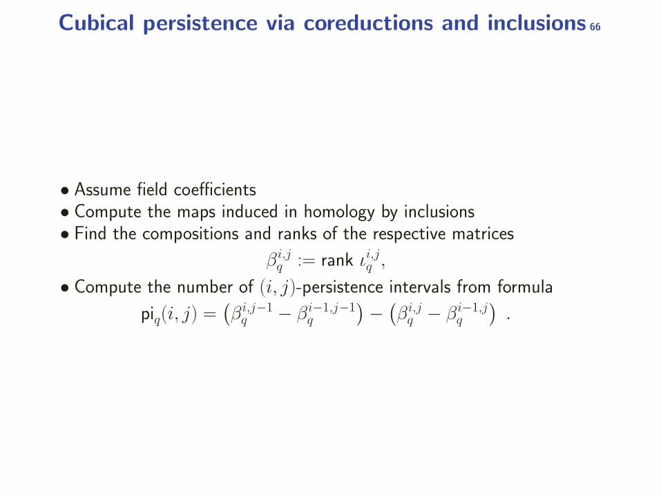
Cubical persistence via coreductions and inclusions 66

• Assume field coefficients• Compute the maps induced in homology by inclusions• Find the compositions and ranks of the respective matrices

βi,jq := rank ιi,jq ,

• Compute the number of (i, j)-persistence intervals from formula

piq(i, j) =(βi,j−1q − βi−1,j−1

q

)− (βi,jq − βi−1,j

q

).

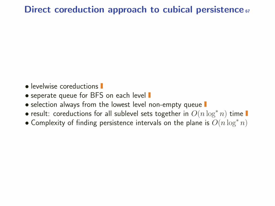
Direct coreduction approach to cubical persistence 67

• levelwise coreductions• seperate queue for BFS on each level• selection always from the lowest level non-empty queue• result: coreductions for all sublevel sets together in O(n log∗ n) time• Complexity of finding persistence intervals on the plane is O(n log∗ n)

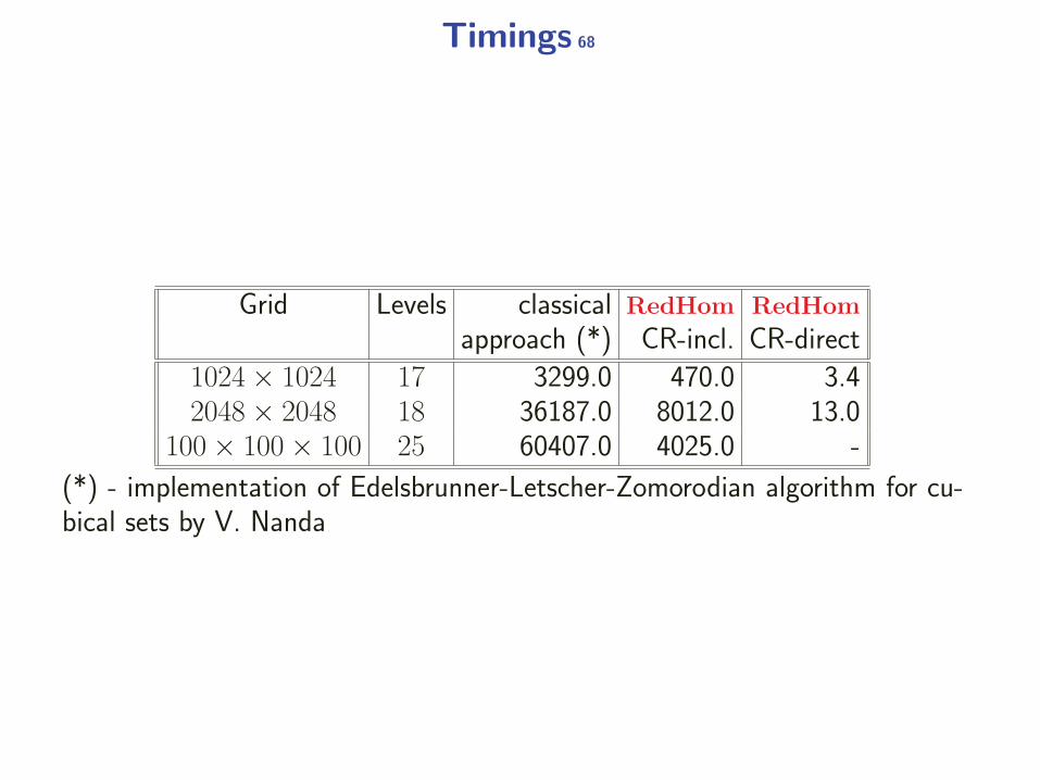
Timings 68

Grid Levels classical RedHom RedHom

approach (*) CR-incl. CR-direct

1024× 1024 17 3299.0 470.0 3.42048× 2048 18 36187.0 8012.0 13.0

100× 100× 100 25 60407.0 4025.0 -

(*) - implementation of Edelsbrunner-Letscher-Zomorodian algorithm for cu-bical sets by V. Nanda

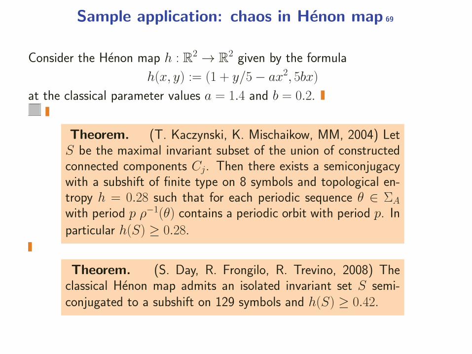
Sample application: chaos in Henon map 69

Consider the Henon map h : R2 → R2 given by the formula

h(x, y) := (1 + y/5− ax2, 5bx)

at the classical parameter values a = 1.4 and b = 0.2.

Theorem. (T. Kaczynski, K. Mischaikow, MM, 2004) LetS be the maximal invariant subset of the union of constructedconnected components Cj. Then there exists a semiconjugacywith a subshift of finite type on 8 symbols and topological en-tropy h = 0.28 such that for each periodic sequence θ ∈ ΣA

with period p ρ−1(θ) contains a periodic orbit with period p. Inparticular h(S) ≥ 0.28.

Theorem. (S. Day, R. Frongilo, R. Trevino, 2008) Theclassical Henon map admits an isolated invariant set S semi-conjugated to a subshift on 129 symbols and h(S) ≥ 0.42.

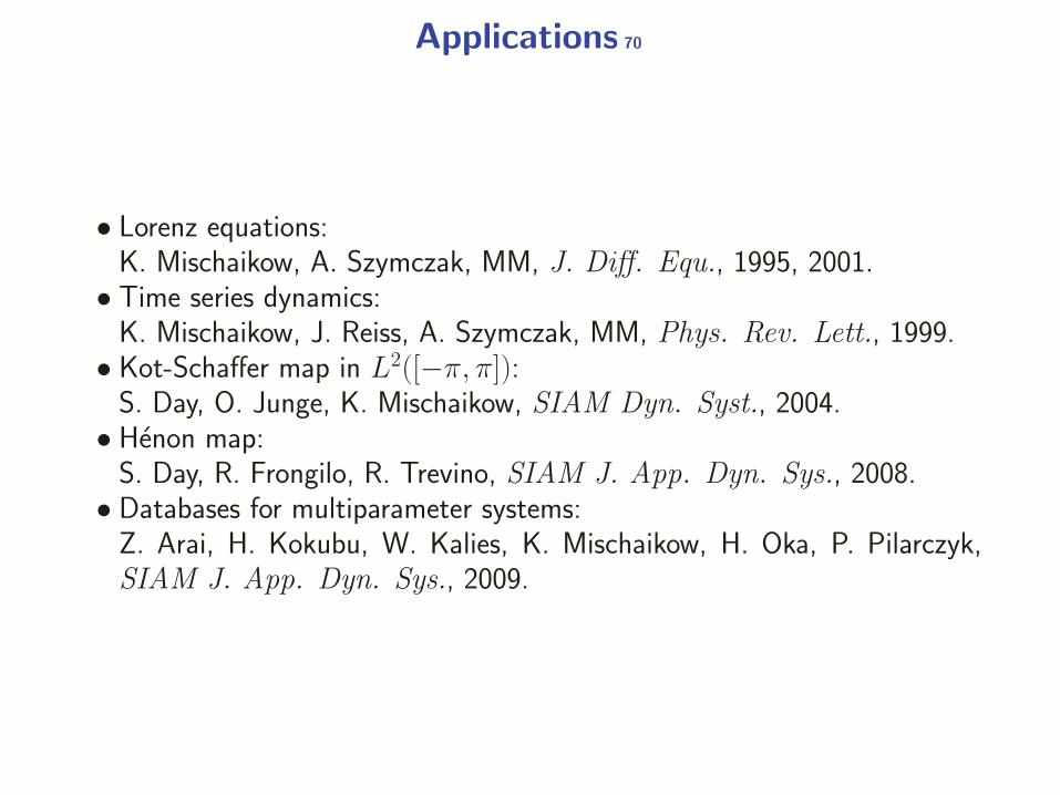
Applications 70

• Lorenz equations:K. Mischaikow, A. Szymczak, MM, J. Diff. Equ., 1995, 2001.

• Time series dynamics:K. Mischaikow, J. Reiss, A. Szymczak, MM, Phys. Rev. Lett., 1999.

• Kot-Schaffer map in L2([−π, π]):S. Day, O. Junge, K. Mischaikow, SIAM Dyn. Syst., 2004.

• Henon map:S. Day, R. Frongilo, R. Trevino, SIAM J. App. Dyn. Sys., 2008.

• Databases for multiparameter systems:Z. Arai, H. Kokubu, W. Kalies, K. Mischaikow, H. Oka, P. Pilarczyk,SIAM J. App. Dyn. Sys., 2009.

Conclusion 71

• Direct algebraization need not be the quickest way to compute homologyof sets and maps.

• Reduction algorithms operating directly on sets substantially speed uphomology copmutations.

• A universal fastest algorithm probably does not exist and hybrid methodsprobing data should be used for best performance.

• There is potential for further improvement in homology computations.

References 72

• MM, P. Pilarczyk, N. Zelazna, Homology algorithm based on acyclic subspace,Computers and Mathematics with Applications (2008).

• MM, B. Batko, Coreduction homology algorithm, Discrete and ComputationalGeometry (2009).

• K. Mischaikow, MM, P. Pilarczyk, Graph Approach to the Computation ofthe Homology of Continuous Maps, Foundations of Computational Mathematics(2005).

• MM, Cech Type Approach to Computing Homology of Maps, Discrete and Compu-tational Geometry (2010).

• M. Juda, MM, Z2-Homology of 2-manifolds may be computed in O(nα(n)) time,preprint (2009).

• P. D�lotko, T. Kaczynski, MM, T. Wanner, Coreduction Homology Algorithmfor Regular CW-Complexes, Discrete and Computational Geometry (accepted).

• MM, T. Wanner, Coreduction Homology Algorithm for Inclusions and Persistence,Computers and Mathematics with Applications (accepted).

• S. Harker, K. Mischaikow, MM, V. Nanda, H. Wagner, M. Juda, P.D�lotko, The Efficiency of a Homology Algorithm based on Discrete Morse Theoryand Coreductions, Proceedings CTIC 2010 (2010).

• MM, H. Wagner, Coreduction Homology Algorithm for Continuous Maps, inpreparation.

• A. Krajniak, MM, T. Wanner, Direct coreduction approach to persistence, inpreparation.