APP

LIED

MA

THEM

ATI

CSD

EVEL

OPM

ENTA

LBI

OLO

GY

Topological data analysis of zebrafish patternsMelissa R. McGuirla,1 , Alexandria Volkeningb, and Bjorn Sandstedea,c

aDivision of Applied Mathematics, Brown University, Providence, RI 02912; bNSF–Simons Center for Quantitative Biology, Northwestern University,Evanston, IL 60208; and cData Science Initiative, Brown University, Providence, RI 02912

Edited by Andrea L. Bertozzi, University of California, Los Angeles, CA, and approved January 29, 2020 (received for review October 21, 2019)

Self-organized pattern behavior is ubiquitous throughout nature,from fish schooling to collective cell dynamics during organismdevelopment. Qualitatively these patterns display impressive con-sistency, yet variability inevitably exists within pattern-formingsystems on both microscopic and macroscopic scales. Quantify-ing variability and measuring pattern features can inform theunderlying agent interactions and allow for predictive analy-ses. Nevertheless, current methods for analyzing patterns thatarise from collective behavior capture only macroscopic featuresor rely on either manual inspection or smoothing algorithmsthat lose the underlying agent-based nature of the data. Herewe introduce methods based on topological data analysis andinterpretable machine learning for quantifying both agent-levelfeatures and global pattern attributes on a large scale. Becausethe zebrafish is a model organism for skin pattern formation,we focus specifically on analyzing its skin patterns as a meansof illustrating our approach. Using a recent agent-based model,we simulate thousands of wild-type and mutant zebrafish pat-terns and apply our methodology to better understand patternvariability in zebrafish. Our methodology is able to quantify thedifferential impact of stochasticity in cell interactions on wild-typeand mutant patterns, and we use our methods to predict stripeand spot statistics as a function of varying cellular communication.Our work provides an approach to automatically quantifying bio-logical patterns and analyzing agent-based dynamics so that wecan now answer critical questions in pattern formation at a muchlarger scale.

topological data analysis | agent-based model | self-organization |pattern quantification | zebrafish

Patterns are widespread in nature and often form due to theself-organization of independent agents. Whether explor-

ing such collective dynamics in cancer (1), wound healing (2),hair growth (3), or skin pattern formation (4, 5), researchersfocus on uncovering unknown cell behavior and signaling usinga combination of experimental and modeling techniques. Thisprocess is complicated by the fact that biological patterns areinherently variable, making it challenging to quantify the distin-guishing features of different mutants and judge model accuracy.In some applications, such as zebrafish skin patterns (Fig. 1A–D), global information about patterns both in vivo and in sil-ico is largely based on visual inspection, and this naturally leadsto more subjectivity and limits the scale of the analyses. More-over, the focus is often on the characteristic features of differentmutants, making it unclear how much variability normally arisesin mutant patterns and how this variability compares to wild type.To help address these challenges, here we develop a method-ology, based on topological data analysis and machine learning,for quantifying self-organized patterns with an automated, agent-based approach, and we apply our methods to study variability inzebrafish skin patterns.

Characterized by black and gold stripes, the zebrafish (Daniorerio) is a model organism in the field of skin pattern formation(4, 6, 7). Remarkably, zebrafish stripes form due to the inter-actions of tens of thousands of different-colored cells, whichreliably self-organize on the growing skin despite their stochas-tic environment (8–10). In addition to their namesake stripes,zebrafish feature a wealth of other patterns [e.g., spots and

labyrinth curves (11)] that form due to genetic mutations thatrestrict cell birth or alter cell behavior (often in unknown ways).While wild-type stripes (Fig. 1A) are considered robust, mutantsthat lack certain cell types (Fig. 1 B–D) feature more variablespotty patterns (11). For example, the nacre phenotype (9, 11,12) has an enlarged central orange region with scattered bluesplotches (Fig. 1B). In comparison, both the pfeffer (9–11, 13) andshady (11, 14) mutants are characterized by dark spots, roughlyaligned in stripes. These patterns differ in their finer details:pfeffer has messy spots and peppered black cells across its skin,while shady has sharp boundaries between light and dark regions(11). Although these descriptions apply in general, patterns varydue to the stochastic nature of pigment cell interactions.

Mathematical descriptions of zebrafish patterns capturestochastic cellular interactions at different levels of detail. Whilepartial differential equations (e.g., refs. 8, 15, and 16) offer abroad perspective on the evolution of cell densities, cellularautomaton (17, 18) and agent-based models (19–21) providea more detailed view of individual cell behavior. For exam-ple, the agent-based model (20) specified cell interactions usingstochastic rules to simulate zebrafish patterning in silico (Fig. 1F–I). Ideally, models should reproduce pattern formation as itis observed in vivo, and this raises the question, How can we

Significance

While pattern formation has been studied extensively usingexperiments and mathematical models, methods for quan-tifying self-organization are limited to manual inspectionor global measures in many applications. Our work intro-duces a methodology for automatically quantifying patternsthat arise due to agent interactions. We combine topologi-cal data analysis and machine learning to provide a collectionof summary statistics describing patterns on both micro-scopic and macroscopic scales. We apply our methodologyto study zebrafish patterns across thousands of model sim-ulations, allowing us to make quantitative predictions aboutthe types of pattern variability present in wild-type andmutant zebrafish. Our work helps address the widespreadchallenge of quantifying agent-based patterns and opens uppossibilities for large-scale analysis of biological data andmathematical models.

Author contributions: M.R.M., A.V., and B.S. designed research; M.R.M. performedresearch; M.R.M. and A.V. contributed new reagents/analytic tools; M.R.M. analyzeddata; and M.R.M. and A.V. wrote the paper.y

The authors declare no competing interest.y

This article is a PNAS Direct Submission.y

This open access article is distributed under Creative Commons Attribution License 4.0(CC BY).y

Data deposition: Implementation details and code are freely available on GitHub: https://github.com/sandstede-lab/Quantifying Zebrafish Patterns. Simulated data are publiclyavailable on Figshare: https://figshare.com/projects/Zebrafish simulation data/72689.High-quality versions of the figures within this article are available on Figshare(https://doi.org/10.6084/m9.figshare.11868249.v1).y

1To whom correspondence may be addressed. Email: melissa mcguirl@brown.edu.y

This article contains supporting information online at https://www.pnas.org/lookup/suppl/doi:10.1073/pnas.1917763117/-/DCSupplemental.y

First published February 25, 2020.

www.pnas.org/cgi/doi/10.1073/pnas.1917763117 PNAS | March 10, 2020 | vol. 117 | no. 10 | 5113–5124

Dow

nloa

ded

by g

uest

on

Aug

ust 2

, 202

0

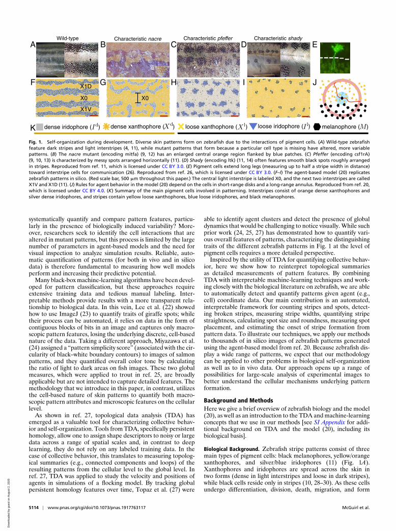
Wild-type Characteristic shadyCharacteristic nacre Characteristic pfefferA B DC

melanophore ( )dense xanthophore ( ) loose xanthophore ( )dense iridophore ( ) loose iridophore ( )

F G IH

E

J

K

X0

X1V

X1D

X0

Fig. 1. Self-organization during development. Diverse skin patterns form on zebrafish due to the interactions of pigment cells. (A) Wild-type zebrafishfeature dark stripes and light interstripes (4, 11), while mutant patterns that form because a particular cell type is missing have altered, more variablepatterns. (B) The nacre mutant (encoding mitfa) (9, 12) has an enlarged central orange region flanked by blue patches. (C) Pfeffer (encoding csf1rA)(9, 10, 13) is characterized by messy spots arranged horizontally (11). (D) Shady (encoding ltk) (11, 14) often features smooth black spots roughly arrangedin stripes. Reproduced from ref. 11, which is licensed under CC BY 3.0. (E) Pigment cells extend long legs (measuring up to half a stripe width in distance)toward interstripe cells for communication (26). Reproduced from ref. 26, which is licensed under CC BY 3.0. (F–I) The agent-based model (20) replicateszebrafish patterns in silico. (Red scale bar, 500 µm throughout this paper.) The central light interstripe is labeled X0, and the next two interstripes are calledX1V and X1D (11). (J) Rules for agent behavior in the model (20) depend on the cells in short-range disks and a long-range annulus. Reproduced from ref. 20,which is licensed under CC BY 4.0. (K) Summary of the main pigment cells involved in patterning. Interstripes consist of orange dense xanthophores andsilver dense iridophores, and stripes contain yellow loose xanthophores, blue loose iridophores, and black melanophores.

systematically quantify and compare pattern features, particu-larly in the presence of biologically induced variability? More-over, researchers seek to identify the cell interactions that arealtered in mutant patterns, but this process is limited by the largenumber of parameters in agent-based models and the need forvisual inspection to analyze simulation results. Reliable, auto-matic quantification of patterns (for both in vivo and in silicodata) is therefore fundamental to measuring how well modelsperform and increasing their predictive potential.

Many black-box machine-learning algorithms have been devel-oped for pattern classification, but these approaches requireextensive training data and tedious manual labeling. Inter-pretable methods provide results with a more transparent rela-tionship to biological data. In this vein, Lee et al. (22) showedhow to use ImageJ (23) to quantify traits of giraffe spots; whiletheir process can be automated, it relies on data in the form ofcontiguous blocks of bits in an image and captures only macro-scopic pattern features, losing the underlying discrete, cell-basednature of the data. Taking a different approach, Miyazawa et al.(24) assigned a “pattern simplicity score” (associated with the cir-cularity of black–white boundary contours) to images of salmonpatterns, and they quantified overall color tone by calculatingthe ratio of light to dark areas on fish images. These two globalmeasures, which were applied to trout in ref. 25, are broadlyapplicable but are not intended to capture detailed features. Themethodology that we introduce in this paper, in contrast, utilizesthe cell-based nature of skin patterns to quantify both macro-scopic pattern attributes and microscopic features on the cellularlevel.

As shown in ref. 27, topological data analysis (TDA) hasemerged as a valuable tool for characterizing collective behav-ior and self-organization. Tools from TDA, specifically persistenthomology, allow one to assign shape descriptors to noisy or largedata across a range of spatial scales and, in contrast to deeplearning, they do not rely on any labeled training data. In thecase of collective behavior, this translates to measuring topolog-ical summaries (e.g., connected components and loops) of theresulting patterns from the cellular level to the global level. Inref. 27, TDA was applied to study the velocity and positions ofagents in simulations of a flocking model. By tracking globalpersistent homology features over time, Topaz et al. (27) were

able to identify agent clusters and detect the presence of globaldynamics that would be challenging to notice visually. While suchprior work (24, 25, 27) has demonstrated how to quantify vari-ous overall features of patterns, characterizing the distinguishingtraits of the different zebrafish patterns in Fig. 1 at the level ofpigment cells requires a more detailed perspective.

Inspired by the utility of TDA for quantifying collective behav-ior, here we show how to reinterpret topological summariesas detailed measurements of pattern features. By combiningTDA with interpretable machine-learning techniques and work-ing closely with the biological literature on zebrafish, we are ableto automatically detect and quantify patterns given agent (e.g.,cell) coordinate data. Our main contribution is an automated,interpretable framework for counting stripes and spots, detect-ing broken stripes, measuring stripe widths, quantifying stripestraightness, calculating spot size and roundness, measuring spotplacement, and estimating the onset of stripe formation frompattern data. To illustrate our techniques, we apply our methodsto thousands of in silico images of zebrafish patterns generatedusing the agent-based model from ref. 20. Because zebrafish dis-play a wide range of patterns, we expect that our methodologycan be applied to other problems in biological self-organizationas well as to in vivo data. Our approach opens up a range ofpossibilities for large-scale analysis of experimental images tobetter understand the cellular mechanisms underlying patternformation.

Background and MethodsHere we give a brief overview of zebrafish biology and the model(20), as well as an introduction to the TDA and machine-learningconcepts that we use in our methods [see SI Appendix for addi-tional background on TDA and the model (20), including itsbiological basis].

Biological Background. Zebrafish stripe patterns consist of threemain types of pigment cells: black melanophores, yellow/orangexanthophores, and silver/blue iridophores (11) (Fig. 1A).Xanthophores and iridophores are spread across the skin intwo forms (dense in light interstripes and loose in dark stripes),while black cells reside only in stripes (10, 28–30). As these cellsundergo differentiation, division, death, migration, and form

5114 | www.pnas.org/cgi/doi/10.1073/pnas.1917763117 McGuirl et al.

Dow

nloa

ded

by g

uest

on

Aug

ust 2

, 202

0

APP

LIED

MA

THEM

ATI

CSD

EVEL

OPM

ENTA

LBI

OLO

GY

changes, they self-organize into four to five stripes and four inter-stripes sequentially over a few months (4). During this time, thefish body grows in length from roughly 7.5 mm to over 16 mm(31). Cells regulate each other’s behavior through communica-tion at short range (between neighboring cells) and at long range(between cells in stripes and interstripes) (e.g., refs. 8, 15, and32–34); see Fig. 1E. Importantly, this regulation is inherentlynoisy. For example, cells may interact by reaching extensionstoward their neighbors (26, 35, 36); whether or not cellular com-munication occurs then depends on whether these extensionssuccessfully find another cell.

Prior models (19, 20) have used estimates of wild-type stripewidth (26, 37) and descriptions of developmental timelines (e.g.,approximate times at which new stripes appear) (4, 31, 38) tojudge model performance or fit parameters. Fewer data areavailable for zebrafish mutants, and, to our knowledge, globalinformation is in the form of qualitative descriptions of the char-acteristic features of their patterns. Local measurements, in turn,include cell speeds (39, 40) and distances between adjacent cells(33, 39, 41). Notably, we are not aware of measurements ofpattern variability or stripe straightness.

Model and Generation of In Silico Pattern Data. The model (20)treats pigment cells as individual agents (point masses) andtracks their positions (namely (x , y) coordinates) in space as theyinteract on growing 2D domains. These domains capture the fullheight of the fish body and one-third of its length (excluding aregion around the eye). The number of agents is carefully basedon empirical measurements of cell–cell distances [roughly 30 to80 µm, depending on the cell type (39)], so that agent dynamicsoccur on the same scale as cell interactions on the fish skin (20).See SI Appendix, Fig. S3 for a summary of the model (20) and thelength scales involved.

The behavior of five different types of cell agents is accountedfor in ref. 20: We let Mi(t) be the (x , y) coordinate of the i thmelanophore (M ) at time t ; similarly, Xd

i (t), Xli(t), Id

i (t), andIli(t) denote the locations of the i th dense xanthophore (X d),

loose xanthophore (X l), dense iridophore (I d), and loose iri-dophore (I l), respectively; see Fig. 1K. Space is continuous, andcell movement, which includes repulsion and attraction, is mod-eled by coupled ordinary differential equations. Cell birth, death,and transitions in type, in turn, take the form of stochastic,discrete-time rules. These rules, which are strongly motivated bythe biological literature (e.g., refs. 11, 15, 34, and 39), dependon the number of cells in disk and annulus neighborhoods cen-tered at the cell or location of interest (Fig. 1J). Volkening andSandstede (20) use these neighborhoods to model the cells that agiven cell (or precursor) could communicate with [e.g., throughdirect contact (42), diffusing substances (34), or dendrite exten-sions (26, 35, 36) as in Fig. 1E]. As an example cell interactionrule, interstripe cells are known to promote M differentiation atlong range (15, 32), and these dynamics are modeled as∑N d

Xi=1 1Ωz

long(Xd

i ) +∑N d

Ii=1 1Ωz

long(Id

i )

α+β∑NM

i=1 1Ωzlong

(Mi)> 1

=⇒ M birth at z (if not overcrowded), [1]

where z is a randomly selected location to be evaluated for pos-sible cell birth; N d

X, N dI , and NM are the numbers of X d, I d,

and M cells on the domain, respectively; and Ωzlong is an annu-

lus centered at z that models long-range cellular communication(Fig. 1J). According to Eq. 1, a new M cell appears at positionz when the ratio of interstripes cells to M cells at long range isgreater than one. [Note that the interaction rules in ref. 20 aregiven in terms of numbers, rather than proportions, of cells. Wehave adjusted the model (20) so that these rules depend on the

ratios or densities of cells in different regions, as this frameworkworks better for our large-scale study; see SI Appendix for moredetails.]

The agent-based model (20) can be used to simulate the fulltimeline of adult pattern formation from when it begins when thefish is roughly 21 days post fertilization (dpf). Because the model(20) is stochastic, simulating it repeatedly leads to different insilico patterns and, importantly, for our methods, cell-coordinatedata. We thus generate an extensive dataset by simulating thedevelopment of thousands of zebrafish patterns. We simulatewild-type development from 21 dpf until 66 dpf, at which pointzebrafish, measuring about 2.2 mm in height and 12.6 mm inbody length (according to the growth rates approximated fromref. 31 in ref. 20), are expected to have three complete inter-stripes, two complete stripes, and some partially formed stripesnear the boundaries (SI Appendix, Fig. S3B). We simulate nacreand pfeffer pattern formation until 76 dpf and shady develop-ment until 96 dpf by turning cell birth off for the appropriatecell types as described in ref. 20. [We note that experimental-ists often use stages (31) rather than dpf to measure time; inthe model (20), 66 dpf, 76 dpf, and 39 to 44 dpf correspond tothe juvenile, juvenile+, and squamation onset posterior stages,respectively.] With one exception, we perform all of our analy-ses on the final simulated patterns at 66 dpf (for wild type), 76dpf (for nacre and pfeffer), and 96 dpf (for shady). Following theapproach in ref. 20, we enforce periodic boundary conditions inthe horizontal direction and wall-like boundary conditions at thetop and bottom of these domains (Fig. 3A). To help avoid quan-tifying partially formed stripes or spots, we remove the cells inthe top and bottom 10% of the domain in postprocessing.

To generate our first dataset, we simulate wild-type, nacre,pfeffer, and shady patterns under the baseline conditions andparameters described in ref. 20. We then adjust the model toaccount for more realistic biological stochasticity in cell interac-tions. In particular, rather than using deterministic length scalesin the cell interaction rules, each day we select these length scalesrandomly per cell and interaction from a normal distribution cen-tered at the default parameter value. In our last dataset, we focuson the inner radius of Ωlong in Eq. 1 and explore the role of thisparameter while keeping all other parameters at their defaultvalues.

Topological Data Analysis and Machine Learning. Our approachto quantifying patterns relies on topological data analysis andmachine learning. TDA is an emerging branch of mathematicsand statistics that aims to extract quantifiable shape invariantsfrom complex and often large data (43–47). One of the maintools in TDA is known as persistent homology, which we reviewnow briefly. Given a dataset of N discrete points xiNi=1 that liein some metric space (D , dD), we place a ball of radius r at eachxi to obtain the set br (xi) = y∈D : dD(xi , y)≤ r. We then takethe union of these balls over all i ∈ [1,N ], namely

⋃i∈[1,N ] br (xi).

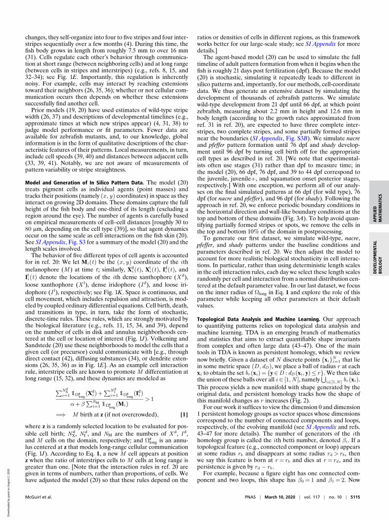
This process yields a new manifold with shape generated by theoriginal data, and persistent homology tracks how the shape ofthis manifold changes as r increases (Fig. 2).

For our work it suffices to view the dimension 0 and dimension1 persistent homology groups as vector spaces whose dimensionscorrespond to the number of connected components and loops,respectively, of the evolving manifold (see SI Appendix and refs.43–47 for more details). The number of generators of the i thhomology group is called the i th betti number, denoted βi . If atopological feature (e.g., connected component or loop) appearsat some radius rb and disappears at some radius rd > rb , thenwe say this feature is born at r = rb and dies at r = rd , and itspersistence is given by rd − rb .

For example, because a figure eight has one connected com-ponent and two loops, this shape has β0 = 1 and β1 = 2. Now

McGuirl et al. PNAS | March 10, 2020 | vol. 117 | no. 10 | 5115

Dow

nloa

ded

by g

uest

on

Aug

ust 2

, 202

0

A B

Fig. 2. Illustration of persistent homology applied to coordinate data.(A and B) Noisy data sampled from a figure-eight shape (A) andcorresponding manifold expansions (B).

consider a noisy dataset sampled from a figure eight, as we showin Fig. 2A. To compute the persistent homology of these data wetake the union of balls of radius r centered around each datapoint for an increasing sequence of r values. Two loops appearin the data at r = r2 and disappear before r = r3 in Fig. 2B, sothis dataset has two dimension 1 homology generators that areboth born at rb = r2 and die at rd = r3 (with persistence given byr3− r2). Similarly, this dataset is connected for r ≥ r2, so it hasone dimension 0 homology generator for r ≥ r2 with infinite per-sistence and several dimension 0 homology generators for r < r2.Thus, persistent homology reveals that the noisy data in Fig. 2Aare topologically similar to a figure-eight shape (β0 = 1, β1 = 2)for r2≤ r < r3.

In addition to using TDA, we apply methods from inter-pretable machine learning to quantify patterns. Machine-learning algorithms seek to automatically learn information froma given dataset for classification or prediction purposes (48, 49).The machine-learning approach we use involves clustering datainto different classes based on a similarity measure. Specifically,we apply single-linkage clustering to subsets of agents (e.g., pig-ment cells) to identify clusters corresponding to spot or stripepatterns. Single-linkage clustering is an agglomerative hierarchi-cal clustering method: Each data point begins in its own clusterand points (or clusters of points) are merged sequentially based

on which two clusters are closest to each other (48, 49). We con-tinue this process until there are n clusters, where n is eitherone or some predetermined number of desirable clusters. Weuse single-linkage clustering over other clustering algorithms(e.g., average linkage or k-means) to capture elongated, undu-lating, and nonspherical clusters that are characteristic of somezebrafish mutants (Fig. 1).

As a side note, dimension 0 persistent homology is analo-gous to single-linkage clustering, so there is a natural connectionbetween TDA- and clustering-based methods for pattern quan-tification (43). Using clustering and topological methods in tan-dem yields both multidimensional, coordinate-free summaries(from TDA) and essential information about the locations ofdifferent agents (from clustering).

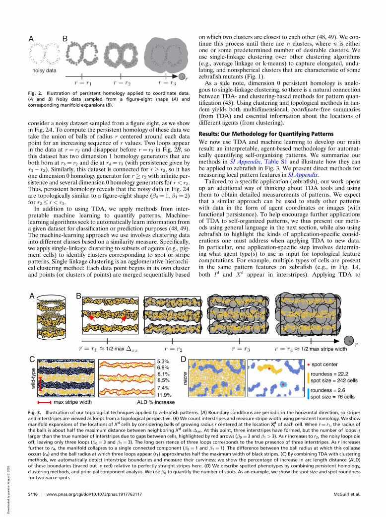
Results: Our Methodology for Quantifying PatternsWe now use TDA and machine learning to develop our mainresult: an interpretable, agent-based methodology for automat-ically quantifying self-organizing patterns. We summarize ourmethods in SI Appendix, Table S1 and illustrate how they canbe applied to zebrafish in Fig. 3. We present direct methods formeasuring local pattern features in SI Appendix.

Tailored to a specific application (zebrafish), our work opensup an additional way of thinking about TDA tools and usingthem to obtain detailed measurements of patterns. We expectthat a similar approach can be used to study other patternswith data in the form of agent coordinates or images (withfunctional persistence). To help encourage further applicationsof TDA to self-organized patterns, we thus present our meth-ods using general language in the next section, while also usingzebrafish to highlight the kinds of application-specific consid-erations one must address when applying TDA to new data.In particular, one application-specific step involves determin-ing what agent type(s) to use as input for topological featurecomputations. For example, multiple types of cells are presentin the same pattern features on zebrafish (e.g., in Fig. 1A,both I d and X d appear in interstripes). Applying TDA to

A B

C D

Fig. 3. Illustration of our topological techniques applied to zebrafish patterns. (A) Boundary conditions are periodic in the horizontal direction, so stripesand interstripes are viewed as loops from a topological perspective. (B) We count interstripes and measure stripe width using persistent homology. We showmanifold expansions of the locations of Xd cells by considering balls of growing radius r centered at the location Xd

i of each cell. When r = r1, the radius ofthe balls is about half the maximum distance between neighboring Xd cells ∆xx . At this point, three interstripes have formed, but the number of loops islarger than the true number of interstripes due to gaps between cells, highlighted by red arrows (β0 = 3 and β1 > 3). As r increases to r2, the noisy loops dieoff, leaving only three loops (β0 = 3 and β1 = 3). The long persistence of three loops corresponds to the true presence of three interstripes. As r increasesfurther to r4, the manifold collapses to a single connected component (β0 = 1 and β1 = 1). The difference between the ball radius at which this collapseoccurs (r4) and the ball radius at which three loops appear (r1) approximates half the maximum width of black stripes. (C) By combining TDA with clusteringmethods, we automatically detect interstripe boundaries and measure their curviness; we show the percentage of increase in arc length distance (ALD)of these boundaries (traced out in red) relative to perfectly straight stripes here. (D) We describe spotted phenotypes by combining persistent homology,clustering methods, and principal component analysis. We use β0 to quantify the number of spots. As an example, we show the spot size and spot roundnessfor two nacre spots.

5116 | www.pnas.org/cgi/doi/10.1073/pnas.1917763117 McGuirl et al.

Dow

nloa

ded

by g

uest

on

Aug

ust 2

, 202

0

APP

LIED

MA

THEM

ATI

CSD

EVEL

OPM

ENTA

LBI

OLO

GY

the locations of every agent type in a pattern is expensive.It may be sufficient to study only one or two agent types,but selecting which types to use requires application-specificconsiderations.

Counting Spots and Stripes. We compute the dimension 0 anddimension 1 persistent homology groups using the coordinatedata of agents [e.g., pigment cell locations generated by themodel (20)] to quantify pattern types, assuming periodic bound-ary conditions in the x direction. With these boundary condi-tions, spots can be viewed as connected components withoutloops, whereas stripes wrap around the domain and are thusconnected components with a single loop (Fig. 3 A and B).Consequently, β0 and β1 approximate the number of spots andstripes in a pattern, respectively.∗

For zebrafish, we estimate the number of stripes and inter-stripes in wild-type patterns by computing β1 for X l and X d

cells, respectively. We apply TDA to these cells because theyuniformly cover the fish skin, but in different forms in stripesand interstripes.† We estimate the number of spots in nacre andpfeffer patterns by computing β0 using the locations of blue I l

cells.‡ For pfeffer, individual M cells appear randomly on thedomain, so using these cells to count the number of spots wouldintroduce spurious connected components (in the form of indi-vidual black cells). In comparison, M are much more clusteredin shady; thus, we calculate the number of dark shady spots bycomputing β0 for M.

In general, we calculate betti numbers by applying persis-tent homology to the agents’ coordinates and using a persis-tence threshold to count the number of homological genera-tors whose persistence is greater than the set threshold (Tp).Empirical estimates of cell–cell spacing motivate our choice ofTp for zebrafish. Specifically, we use T 0

p = 100 µm and T 0p =

90 µm as the dimension 0 persistence thresholds for iridophoresand melanophores, respectively. We chose these thresholdsconservatively, as average xanthophore–xanthophore neighbor-ing distances are 30 to 60 µm and average melanophore–melanophore distances are roughly 50 to 60 µm in wild type(20, 33, 39, 41). (We are not aware of empirical measure-ments of iridophore spacing.) For dimension 1 homology, weuse a universal persistence threshold of T 1

p = 200 µm. More-over, to ensure that we correctly differentiate between completeand broken stripes or interstripes, we specify that a persis-tence generator counts toward β1 only if its birth radius rbis below a certain threshold (T 1

b ). For X l and X d, we useT 1

b = 100 µm and T 1b = 80 µm, respectively. These thresholds

were motivated by cell–cell distance measures (33, 39, 41) andtuned based on parameter fitting experiments with stripe andinterstripe breaks.

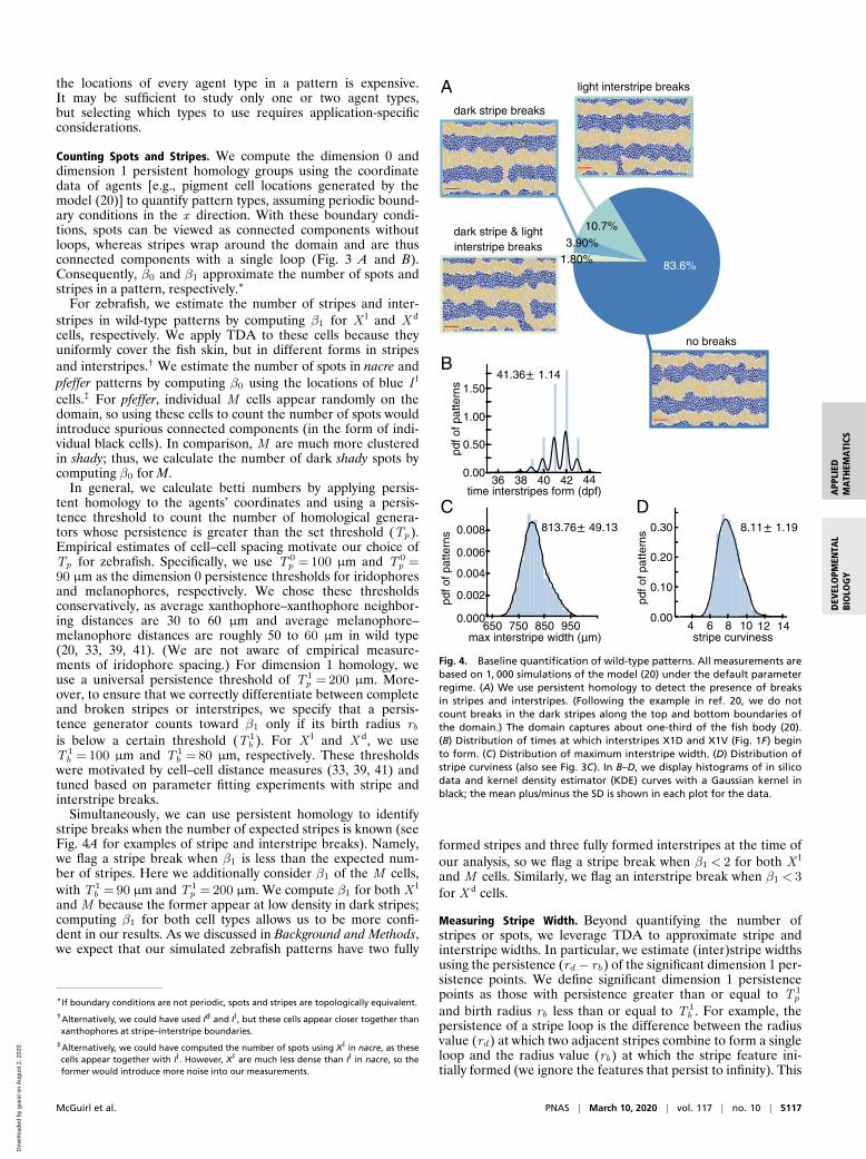
Simultaneously, we can use persistent homology to identifystripe breaks when the number of expected stripes is known (seeFig. 4A for examples of stripe and interstripe breaks). Namely,we flag a stripe break when β1 is less than the expected num-ber of stripes. Here we additionally consider β1 of the M cells,with T 1

b = 90 µm and T 1p = 200 µm. We compute β1 for both X l

and M because the former appear at low density in dark stripes;computing β1 for both cell types allows us to be more confi-dent in our results. As we discussed in Background and Methods,we expect that our simulated zebrafish patterns have two fully

* If boundary conditions are not periodic, spots and stripes are topologically equivalent.†Alternatively, we could have used Id and Il, but these cells appear closer together thanxanthophores at stripe–interstripe boundaries.

‡Alternatively, we could have computed the number of spots using Xl in nacre, as thesecells appear together with Il. However, Xl are much less dense than Il in nacre, so theformer would introduce more noise into our measurements.

light interstripe breaks

dark stripe & light interstripe breaks

no breaks

dark stripe breaks

83.6%

3.90%

10.7%

1.80%

10 120.00

0.10

0.20

0.30

144 6 8stripe curviness

650 750 850 9500.000

0.002

0.004

0.006

0.008

max interstripe width ( m)

pdf o

f pat

tern

s

36 38 40 420.00

0.50

1.00

1.50

44time interstripes form (dpf)

pdf o

f pat

tern

s

41.36 1.14

813.76 49.13 8.11 1.19

pdf o

f pat

tern

s

A

B

C D

Fig. 4. Baseline quantification of wild-type patterns. All measurements arebased on 1, 000 simulations of the model (20) under the default parameterregime. (A) We use persistent homology to detect the presence of breaksin stripes and interstripes. (Following the example in ref. 20, we do notcount breaks in the dark stripes along the top and bottom boundaries ofthe domain.) The domain captures about one-third of the fish body (20).(B) Distribution of times at which interstripes X1D and X1V (Fig. 1F) beginto form. (C) Distribution of maximum interstripe width. (D) Distribution ofstripe curviness (also see Fig. 3C). In B–D, we display histograms of in silicodata and kernel density estimator (KDE) curves with a Gaussian kernel inblack; the mean plus/minus the SD is shown in each plot for the data.

formed stripes and three fully formed interstripes at the time ofour analysis, so we flag a stripe break when β1 < 2 for both X l

and M cells. Similarly, we flag an interstripe break when β1 < 3

for X d cells.

Measuring Stripe Width. Beyond quantifying the number ofstripes or spots, we leverage TDA to approximate stripe andinterstripe widths. In particular, we estimate (inter)stripe widthsusing the persistence (rd − rb) of the significant dimension 1 per-sistence points. We define significant dimension 1 persistencepoints as those with persistence greater than or equal to T 1

p

and birth radius rb less than or equal to T 1b . For example, the

persistence of a stripe loop is the difference between the radiusvalue (rd ) at which two adjacent stripes combine to form a singleloop and the radius value (rb) at which the stripe feature ini-tially formed (we ignore the features that persist to infinity). This

McGuirl et al. PNAS | March 10, 2020 | vol. 117 | no. 10 | 5117

Dow

nloa

ded

by g

uest

on

Aug

ust 2

, 202

0

difference (rd − rb) is half of the maximum distance between twoadjacent stripes, capturing the maximum width of the enclosedinterstripe (Fig. 3).

In wild-type zebrafish, twice the persistence of the yellow X l

loops yields an approximation for the maximum interstripe widthacross the fish. Similarly, twice the persistence of the orangeX d loops approximates an upper bound on stripe width. Wenote that rd alone could be used as an alternative estimate formaximum (inter)stripe width, but we use rd − rb to account forthe narrow boundary region between stripes and interstripes.To obtain a lower bound on stripe width, one could calculatethe persistence of the significant dimension 0 persistence points,as this measurement is based on half of the minimum distancebetween two adjacent interstripes.

Measuring Spot Size. We measure spot size by applying single-linkage hierarchical clustering to the agents of interest with thenumber of desired clusters (e.g., number of spots) set to theβ0 values we obtained from our topological analyses. Then, wecount the number of cells per cluster to approximate the size ofeach spot. We define “spot size” as the median number of agentsper spot across all of the spots.

Quantifying Stripe Straightness. To measure “stripe curviness” wecompute the arc length distance (ALD) of the boundary of eachsingle-linkage cluster that corresponds to a stripe. We define ourstripe curviness measure to be the average percentage of increaseof this ALD from the ALD of straight stripes:

curviness = meanstripes

((true ALD

straight ALD− 1

)× 100

). [2]

For example, to measure the curviness of wild-type zebrafishstripes, we apply single-linkage clustering to the locations of X d

cells. For the number of desirable clusters n , we use the num-ber of expected interstripes minus the number of stripe breaksthat we identified with persistent homology (Fig. 3C). We thencalculate the ALD for the resulting clusters and compute stripecurviness using Eq. 2.

Quantifying Spot Roundness. To estimate spot uniformity, we usethe clusters identified via single-linkage hierarchical clustering(with the number of desired clusters set to the β0 values). Wethen apply principal component analysis (PCA) to each clus-ter. The eigenvalue decomposition in PCA provides informationabout how varied the data are in each dimension. Since our dataare 2D, we use PCA to evaluate the spread of each cluster in thex and y directions. If a spot has significantly more variance in onedirection, this indicates that it is irregularly shaped or elongated.Specifically, we define our roundness measure as

roundness of spots = medianspots

(PCA eigenvalue 1PCA eigenvalue 2

). [3]

We assume that a PCA eigenvalue ratio close to one impliesround spots, while a PCA eigenvalue ratio 1 indicatesirregular, nonuniform spots (see Fig. 3D for examples).

Determining Spot Alignment and Center Width. We quantify spotalignment by first applying single-linkage hierarchical cluster-ing to agent locations (with the number of desired clusters setto the β0 values). We then calculate the pairwise l∞ distancesbetween the cluster centroids and complete a nearest-neighborsearch with the l∞ metric.§ This allows us to extract the distance

§Note that dl∞ ((x1, y1), (x2, y2)) = max(|x1 − x2|, |y1 − y2|).

from each spot to its closest neighboring spot. We define thespot-spacing variance as the SD of these nearest-neighbor l∞ dis-tances. A large spacing variance corresponds to nonuniform spotplacement, while a small spacing variance predicts well-alignedspots.

Motivated by the nacre and shady patterns, which featureexpanded light central regions (Fig. 1 G and I), we also usethe cluster centroids to approximate the center width, definedas twice the distance from the midpoint of the domain to its firstspot. In particular, we estimate the center width as twice the min-imum distance from the cluster centroids to the midpoint of thedomain, minus the median spot diameter. Here we define spotdiameter as twice the greatest Euclidean distance from the spot’scentroid to cells belonging to the spot. For zebrafish, the cen-ter radius corresponds to the width of the central interstripe X0(Fig. 1 F and G).

Capturing Pattern Formation Events. Thus far, we have focusedon quantifying pattern features at a snapshot in time. However,for self-organization that occurs during organism development,it is also useful to estimate the time at which specific featuresemerge. For example, in wild-type zebrafish, the second andthird interstripes X1V and X1D (Fig. 1F) develop around 39to 44 dpf [based on approximations (20) of images in refs. 11and 31]. This information on target time dynamics serves as anadditional quantitative measurement that can be used to evalu-ate models. Here we present a method for quantifying the timeat which stripes X1V and X1D form; future work could extendthese methods to capture the time dynamics of spot formationand other features.

Given data in the form of agent locations at consecutive timepoints, we first assume new stripes form somewhere between dayd0 and d1. If there is no prior knowledge about the expected timeof stripe development, one can set d0 and d1 to the first and lastdays of pattern development, respectively. For zebrafish, becausethe model (20) was parameterized so that interstripes X1D andX1V form around 39 to 44 dpf, we conservatively set d0 = 32 dpfand d1 = 62 dpf. Within the specified time interval, we then ana-lyze the patterns sequentially beginning at d0, assuming there isinitially a single stripe on the domain. At each time step, we findthe upper and lower bounds of the stripes by computing the max-imum and minimum, respectively, of the y coordinates of theagents of interest (e.g., for zebrafish, we use X d cells). Finally,we estimate the initial formation of new stripes as the first day atwhich the upper or lower bounds of the stripes increase by morethan some threshold from the previous day. For zebrafish, thethreshold we use is 200 µm¶ .

Results: A Quantitative Study of Zebrafish PatternsWe now study zebrafish pattern variability and robustness byanalyzing thousands of in silico wild-type and mutant patternsgenerated using the agent-based model (20). Quantitativelyevaluating data of this scale is possible because of our auto-mated framework. As a baseline test, we begin by illustratingour techniques on simulations of wild-type zebrafish stripes.Because our analysis there is consistent with previous charac-terizations collected visually and local pattern measurements,we then use our methods to extract quantifiable features frommutant patterns and measure pattern variability in the presenceof increased stochasticity in cell interactions. We conclude byshowing how our methods can be used to detect the impact ofchanging a given model parameter without the need for visualinspection.

¶Alternatively, we could rely on topological summaries to approximate the initial for-mation of new stripes, but a direct approach is more computationally efficient in thissetting.

5118 | www.pnas.org/cgi/doi/10.1073/pnas.1917763117 McGuirl et al.

Dow

nloa

ded

by g

uest

on

Aug

ust 2

, 202

0

APP

LIED

MA

THEM

ATI

CSD

EVEL

OPM

ENTA

LBI

OLO

GY

We view our results in the next sections as presenting abroader, more objective picture of the behavior of the agent-based model (20). Additionally, because this model is closelybased on the biological literature, our results serve to predictthe kind of pattern variability we expect to see in vivo based onthe model (20). As large-scale collections of experimental imagesbecome available, our predictions can be tested by applying ourtechniques to in vivo images of zebrafish as well.

Illustrating Our Techniques on Wild-Type Zebrafish. We focus onstripes first because they provide a means of testing our method-ology, as wild-type patterns have the most experimental data(collected both in silico and in vivo) available for compari-son. Here we use our methodology to evaluate 1, 000 wild-typezebrafish patterns generated with the model (20) under thedefault parameter regime. Previously, model performance (20)was judged by manually counting the number of stochastic sim-ulations that display breaks (or interruptions) in interstripes andrequiring matches in pattern features (e.g., number of inter-stripes present) at major developmental timepoints. In particu-lar, by inspecting 100 in silico patterns, Volkening and Sandstede(20) reported a success rate of 89% according to the former goal,meaning that 89 of 100 simulations had no interruptions in inter-stripes. (Note that breaks in black stripes are occasionally seenon real fish, so these interruptions were not quantified in ref. 20.)Our methodology allows us to analyze much larger datasets andremove any human error from the process; we demonstrate howtopological methods can be used to detect stripe breaks automat-ically in Fig. 4A. Across 1, 000 wild-type simulations, we find that87.5% have no breaks in interstripes (flagged by a decrease in β1

for X d cells). This agrees well with the success rate in ref. 20 thatwas computed using visual inspection.

As an additional evaluation, we manually viewed 200 modeloutputs and found that the betti numbers capture interstripebreaks with 100% accuracy and only one false positive. In a sim-ilar vein, the model (20) was parameterized so that interstripesX1D and X1V (Fig. 1F) form between 39 and 44 dpf, but untilnow this property was judged by visual inspection. Using ourautomated methods, we show the distribution of times at whichthese interstripes develop in Fig. 4B and find good agreementwith the target pattern milestones in ref. 20.

Fig. 4 C and D shows the distributions of interstripe width andstripe curviness across 1, 000 wild-type simulations. The maxi-mum interstripe width, measured by the persistence of the signif-icant dimension 1 persistence points of X l, represents the maxi-mum separation between adjacent stripes. We find that thisquantity has a mean of about 814 µm and a SD of approxi-mately 49 µm, which is similar to the average distance betweencells (39, 41), suggesting that the average number of cells acrossthe width of a stripe varies by ±1 cell along a stripe. Similarly,in Fig. 4D, we show measurements of wild-type stripe curviness(Eq. 2), a dimensionless quantity that could be compared toempirical data in the future. More generally, Fig. 4 B and D pro-vides a baseline measurement of the model output (20) that weuse to compare to further studies.

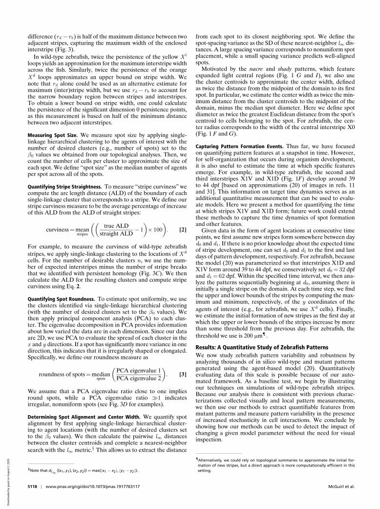
Quantifying “Characteristic” in Noisy Mutant Patterns. The nacre,pfeffer, and shady mutants lack specific cell types, leading toaltered patterns, which are highly variable and can be broadlydescribed as spotty (Fig. 1 B–D). Here we use our methods toanalyze 1, 000 in silico patterns generated with the model (20)under the default parameter regime for each mutant. Our results,shown in Fig. 5, serve as quantitative descriptors of what consti-tutes “characteristic” for each mutant (according to the model)and demonstrate our methods’ abilities to extract quantifiabledifferences between spot patterns. Among the three mutants, wefind that pfeffer has the most spots and that these spots are themost round and the most evenly spaced (Fig. 5 A and C–D). In

pdf o

f pat

tern

spd

f of p

atte

rns

number of spots

0.6

0.5

0.4

0.3

0.2

0.1

0.00 302010

16.15 2.3823.18 1.7516.80 2.54

0.008

0.006

0.004

0.002

0.000

X0 interstripe width ( m) 1200800

744.23 404.91456.77 60.23616.47 93.43

pdf o

f pat

tern

s

0.016

0.012

0.008

0.004

0.000

spot spacing variance ( m)400 800

Nacre Pfeffer Shady

788.56 135.23667.74 26.06903.12 47.43

A B

C D

E

4.36 5.462.21 0.632.85 1.02

1.0

0.8

0.6

0.4

0.2

0.0

spot roundness0 105 15 20

0.20

0.15

0.10

0.05

0.00

spot size (# cells)0 604020 80 100

38.54 10.9424.71 5.3715.88 2.53

Fig. 5. Baseline study of mutant patterns to extract quantifiable features.All measurements are based on 1, 000 simulations of the model (20) (foreach mutant) under the default parameters. Histograms show distributionsfor (A) the number of spots, (B) spot size, (C) spot roundness, (D) variance inspot spacing, and (E) X0 interstripe width (Fig. 1G). We overlay KDE curveswith a Gaussian kernel on the histograms; the mean plus/minus the SD isshown in each plot for the data.

comparison, nacre and shady have a similar number of spots, butthe spots on shady are smaller and rounder than those of nacre.(As we noted in Background and Methods, we remove a smallregion at the top and bottom of the domain prior to our analysisto avoid quantifying partial spots.) Moreover, the width of thecentral X0 interstripe in pfeffer is closest to wild-type interstripewidth (Fig. 4C), while both nacre and shady feature expandedcentral interstripes, echoing empirical observations (11). Inter-estingly, we find that the variance in the number of spots for allthree mutants is small (a SD of about two spots). With the excep-tion of nacre, which displays the greatest variability in four ofthe five measurements we present in Fig. 5, the variance in spotspacing and the width of the central interstripe X0 is also small[on the order of the distance between neighboring cells (39)]. Inthe future, it would be interesting to compare these quantities tolarge-scale in vivo data and determine what cell interactions inthe model (20) are responsible for selecting them robustly.

Measuring Pattern Variability. Some cellular interactions on thezebrafish skin are thought to be regulated by direct contact, den-drites, or longer projections (26, 35, 36) (Fig. 1E). To account forthis, the model (20) assigns disk (short-range communication)and annulus (long-range communication) interaction neighbor-hoods to each cellular agent (Fig. 1J). Cell birth, death, andform transitions are then governed by rules (e.g., Eq. 1) that

McGuirl et al. PNAS | March 10, 2020 | vol. 117 | no. 10 | 5119

Dow

nloa

ded

by g

uest

on

Aug

ust 2

, 202

0

depend on the proportion of cells within these neighborhoods.The size of the neighborhoods dictates which cells are able tointeract and therefore plays a critical role in patterning. Whilethe interaction neighborhoods have deterministic sizes [based onempirical measurements (26, 36, 39)] in ref. 20, a more realisticmodel should account for stochastic variations in cell size andprojection length. Randomly varying the length scales involvedin the interaction neighborhoods serves as a means of includingmore realistic cellular communication [which could also includediffusion of signaling factors (34) in the future] in agent-basedmodels of zebrafish. As a first step toward including more real-istic stochasticity, we therefore replace the deterministic lengthscales in the model (20) with stochastic length-scale parametersand measure their effect on pattern variability. This models thepresence of randomness in cell interactions due to variations incell size and projection length.

Interaction neighborhoods appear in 17 places in the rulesthat govern M birth, M death, iridophore form changes, andxanthophore form changes in the model (20). For each cellinteraction, we randomly select the size of the associated inter-action neighborhood per cell per day from a normal distributionwith the mean set to the default parameter value. We vary theSD from 1 to 50% of the mean and for each SD (we con-sider σ ∈0.01, 0.05, 0.1, 0.2, 0.3, 0.5, where σ times the defaultlength scale is the SD of the normal distribution), we run 1, 000

simulations each for wild type, nacre, pfeffer, and shady.# Ourgoal in this study is twofold: First, we aim to make quantita-tive predictions comparing variability in wild-type and mutantpatterns, and second, we seek to identify the range of patternsthese fish may display in the presence of stochastic cellularcommunication.

To quantitatively explore how additional stochasticity impactspatterning, we first need to define what it means for a patternto look the same as (or different from) what we would expectcharacteristically. For wild type, this is immediate: We charac-terize wild-type patterns in terms of stripe and interstripe breaks.For nacre, pfeffer, and shady, however, the process is more chal-lenging because these mutant patterns are messier. For example,from looking at the images of nacre in Fig. 1 B and G, it is notclear at what point in silico patterns consisting of elongated,orange globs should be considered good or bad matches fornacre. This is where our baseline analysis of nacre, pfeffer, andshady plays a role. We use our earlier analysis of simulations inthe default parameter regime to identify patterns that fall outsideof what constitutes “characteristic” for each of these mutants(in terms of number and size of spots). For each mutant, weset our thresholds for small and large spots to be the minimumand maximum values, respectively, of the cluster-size measuresthat we found in our baseline experiments with that mutant.Analogously, for each mutant, we set the threshold for whatconstitutes few (many) spots to be the minimum (maximum)number of spots we found in our baseline simulations with thatmutant.

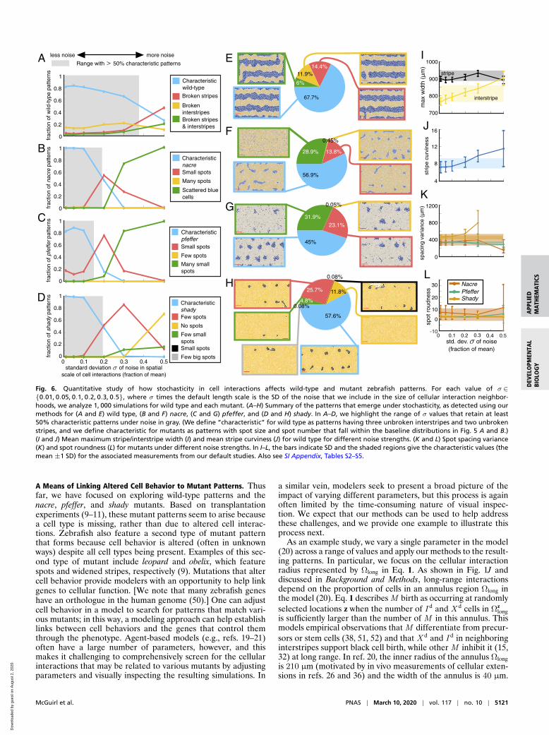
In Fig. 6 A–D, we show how prevalent various patterns areacross our stochastic simulations for different levels of noise incell-interaction length scales (see SI Appendix, Tables S2–S5 foradditional measurements). As an agglomerate summary acrossall 6, 000 simulations that we generated for different σ values,Fig. 6 E–H provides examples of the different patterns cate-gorized by our methods for wild type and each mutant. Ourresults in Fig. 6 A–D suggest that wild-type and mutant patternsbehave differently in the presence of noise. In particular, all threemutants have characteristic spots in less than 50% of the modeloutputs when σ≥ 0.2, while wild-type patterns retain character-

#When we add noise to the annulus parameters, we choose both the inner radius andthe annulus width from a normal distribution.

istic unbroken stripes and interstripes more robustly. If we takea closer look at individual pattern features in Fig. 6 I and J, wenote that low levels of noise (σ≤ 0.1) serve to straighten stripesand that stripe width is mostly unaffected by the inclusion ofnoise in cell size and projection length. As stochasticity increases,wild-type patterns display a gradual decay in quality over therange of σ values that we consider. With increasing noise, we findmore breaks in interstripes, wider interstripes, curvier stripes,and marginally slower pattern formation (SI Appendix, Table S2).Wild-type stripes do not appear to completely deviate from char-acteristic until σ= 0.5, at which point broken stripes becomethe norm.

In comparison, the mutant patterns are almost unaffected bynoise for σ≤ 0.1, but then undergo a sharp change in patternfeatures as σ increases. When nacre and pfeffer stray from char-acteristic, we mostly observe small spots or scattered cells (Fig. 6B and C). Noisy length scales in shady, in turn, generally pro-duce patterns with few or no dark spots (Fig. 6D). Related,Frohnhofer et al. (11) observed that strong forms of the shadymutant have no spots. As we show in Fig. 6 B–D and SI Appendix,Tables S3–S5, spots on all three mutants retain their character-istic roundness across a range of σ values, deviating substantiallyfrom the measures in Fig. 5 only when σ= 0.5.

To roughly approximate the amount of noise present in cel-lular length scales in vivo, we estimate the SD reported for thedistance between neighboring xanthophores (33) and the lengthof their filopodia extensions (30). Based on graphs in ref. 33,we estimate that the distance between the centers of neighbor-ing X d cells (at 40 dpf) is 27 µm with a SD of 4.6 µm; in ournotation, this means that σ= 4.6/27, so the SD is about 17% ofthe mean. Similarly, using graphs in the supporting informationof ref. 30, we estimate that the longest xanthophore extensions(measured from the cell center) have a SD in length that cor-responds to 12% and 20% of the mean filopodia lengths beforeand after iridophores arrive on the skin, respectively (in partic-ular, we find that the filopodia length before iridophores arriveis approximately 58 µm ± 6.7 µm, and the filopodia length afteriridophores arrive is approximately 25 µm ± 5 µm). These mea-surements suggest that focusing on the patterns that emergewhen σ is between roughly 0.1 and 0.2 in our simulations mayhave particular biological relevance. We caution that this approx-imation is based on variance in short-range length scales only,and cells may also communicate through long-range projections(26, 36) [as well as diffusion of signaling molecules (34)]; more-over, in comparing these measurements to our simulations, weare inherently assuming that the empirical data have a normaldistribution.

Motivated by our estimates of SD in vivo, we explore what ouranalysis predicts when σ ∈ [0.1, 0.2]. As we note in SI Appendix,Table S2, we find that wild-type stripe width, stripe curviness, andthe time of formation of interstripes X1V and X1D are robust inthis range of σ. Our methods allow us to estimate that 84.8%and 78.1% of the wild-type patterns for σ= 0.1 and σ= 0.2,respectively, feature characteristic unbroken interstripes (recallthat 87.5% of our simulations in the baseline experiments withσ= 0 have unbroken interstripes). Echoing empirical observa-tions (11) that mutant patterns are more variable than wild type,we find that the model (20) supports a distribution of mutantpatterns for σ ∈ [0.1, 0.2]. In particular, we predict that the rep-resentative images of nacre, pfeffer, and shady in Fig. 1 B–Dand F–H are characteristic of these mutants in the sense thatroughly half of the associated fish may resemble them, whilewe expect that the remaining fish resemble versions of theseimages with fewer and smaller spots. Crucially, we predict thatthe mutants do not commonly display larger spots than thosein Fig. 1 F–H. In the future, analyzing extensive collections ofempirical images will allow one to test our predictions and themodel (20).

5120 | www.pnas.org/cgi/doi/10.1073/pnas.1917763117 McGuirl et al.

Dow

nloa

ded

by g

uest

on

Aug

ust 2

, 202

0

APP

LIED

MA

THEM

ATI

CSD

EVEL

OPM

ENTA

LBI

OLO

GY

less noise more noise

0

0.2

0.4

0.6

0.8

1

frac

tion

of w

ild-t

ype

patte

rns

0.50

0.2

0.4

0.6

0.8

1

frac

tion

of s

hady

pat

tern

s

0

0.2

0.4

0.6

0.8

1

frac

tion

of p

feffe

r pa

ttern

s

0

0.2

0.4

0.6

0.8

1

frac

tion

of n

acre

pat

tern

s

0 0.3 0.4standard deviation of noise in spatial

scale of cell interactions (fraction of mean)

0.1 0.2

Range with 50% characteristic patterns

Characteristicwild-type

Broken stripes

Broken interstripesBroken stripes & interstripes

Characteristic nacreSmall spots

Many spots

Scattered blue cells

Characteristic shadyFew spots

No spots

Few small spotsSmall spots

Few big spots

57.6%

25.7% 11.8%

0.08%

45%

0.05%

23.1%

Few spots

Many small spots

Characteristic pfefferSmall spots

6%

67.7%

14.4%11.9%

28.9%

56.9%

13.8%

0.45%

31.9%

4.8%0.08%

4

8

12

16

strip

e cu

rvin

ess

-10

0

10

20

30

spot

rou

dnes

s

0 0.1 0.2 0.3 0.4 0.5std. dev. of noise (fraction of mean)

0

400

800

1200

spac

ing

varia

nce

(m

)

700

800

900

1000

max

wid

th (

m)

stripe

interstripe

NacrePfefferShady

A

B

D

C

E

G

I

H

F J

L

K

Fig. 6. Quantitative study of how stochasticity in cell interactions affects wild-type and mutant zebrafish patterns. For each value of σ∈0.01, 0.05, 0.1, 0.2, 0.3, 0.5, where σ times the default length scale is the SD of the noise that we include in the size of cellular interaction neighbor-hoods, we analyze 1, 000 simulations for wild type and each mutant. (A–H) Summary of the patterns that emerge under stochasticity, as detected using ourmethods for (A and E) wild type, (B and F) nacre, (C and G) pfeffer, and (D and H) shady. In A–D, we highlight the range of σ values that retain at least50% characteristic patterns under noise in gray. (We define “characteristic” for wild type as patterns having three unbroken interstripes and two unbrokenstripes, and we define characteristic for mutants as patterns with spot size and spot number that fall within the baseline distributions in Fig. 5 A and B.)(I and J) Mean maximum stripe/interstripe width (I) and mean stripe curviness (J) for wild type for different noise strengths. (K and L) Spot spacing variance(K) and spot roundness (L) for mutants under different noise strengths. In I–L, the bars indicate SD and the shaded regions give the characteristic values (themean ±1 SD) for the associated measurements from our default studies. Also see SI Appendix, Tables S2–S5.

A Means of Linking Altered Cell Behavior to Mutant Patterns. Thusfar, we have focused on exploring wild-type patterns and thenacre, pfeffer, and shady mutants. Based on transplantationexperiments (9–11), these mutant patterns seem to arise becausea cell type is missing, rather than due to altered cell interac-tions. Zebrafish also feature a second type of mutant patternthat forms because cell behavior is altered (often in unknownways) despite all cell types being present. Examples of this sec-ond type of mutant include leopard and obelix, which featurespots and widened stripes, respectively (9). Mutations that altercell behavior provide modelers with an opportunity to help linkgenes to cellular function. [We note that many zebrafish geneshave an orthologue in the human genome (50).] One can adjustcell behavior in a model to search for patterns that match vari-ous mutants; in this way, a modeling approach can help establishlinks between cell behaviors and the genes that control themthrough the phenotype. Agent-based models (e.g., refs. 19–21)often have a large number of parameters, however, and thismakes it challenging to comprehensively screen for the cellularinteractions that may be related to various mutants by adjustingparameters and visually inspecting the resulting simulations. In

a similar vein, modelers seek to present a broad picture of theimpact of varying different parameters, but this process is againoften limited by the time-consuming nature of visual inspec-tion. We expect that our methods can be used to help addressthese challenges, and we provide one example to illustrate thisprocess next.

As an example study, we vary a single parameter in the model(20) across a range of values and apply our methods to the result-ing patterns. In particular, we focus on the cellular interactionradius represented by Ωlong in Eq. 1. As shown in Fig. 1J anddiscussed in Background and Methods, long-range interactionsdepend on the proportion of cells in an annulus region Ωlong inthe model (20). Eq. 1 describes M birth as occurring at randomlyselected locations z when the number of I d and X d cells in Ωz

longis sufficiently larger than the number of M in this annulus. Thismodels empirical observations that M differentiate from precur-sors or stem cells (38, 51, 52) and that X d and I d in neighboringinterstripes support black cell birth, while other M inhibit it (15,32) at long range. In ref. 20, the inner radius of the annulus Ωlongis 210 µm (motivated by in vivo measurements of cellular exten-sions in refs. 26 and 36) and the width of the annulus is 40 µm.

McGuirl et al. PNAS | March 10, 2020 | vol. 117 | no. 10 | 5121

Dow

nloa

ded

by g

uest

on

Aug

ust 2

, 202

0

1.2

1

0.8

0.6

20

15

10

5

30

25

20

15

10

5

0

120

100

80

60

40

20

8

6

4

2

0st

ripe

curv

ines

s

max

inte

rstr

ipe

wid

th (

mm

)

num

ber

of s

pots

spot

siz

e (#

cel

ls)

spot

rou

ndne

ss

300200100 400

0

scal

e of

long

-ran

ge in

tera

ctio

ns in

mel

anop

hore

birt

h (

m)

35 m

1.2

1

0.8

0.6

max

str

ipe

wid

th (

mm

) = 1.97 + 487.95

= 0.912

= 1.71 + 471.76

= 0.812

interaction scale in M birth ( m)

300200100 400interaction scale in M birth ( m)

= 0.24

29.72

= 0.902

= 0.37 46.36

= 0.722

300200100 400interaction scale in M birth ( m)

300200100 400interaction scale in M birth ( m)

300200100 400interaction scale in M birth ( m)

300200100 400interaction scale in M birth ( m)

PfefferShady

Wild-type

Default

110 m

210 m

285 m

385 m

Wild-type ShadyPfefferA B C

D E F

G

Fig. 7. Quantifying in silico pattern dependence on the spatial scale of long-range cellular interactions involved in M birth. (A–F) Kernel density estimatesfor (A and B) maximum stripe and interstripe width for wild type, (C) wild-type stripe curviness, (D) number of spots for pfeffer and shady, (E) median spotsize for the mutants, and (F) pfeffer and shady spot roundness as a function of the inner radius of the Ωlong neighborhood in Eq. 1. Measurements in A–F arebased on 100 simulations of the model (20) (for wild type, pfeffer, and nacre, respectively) for each inner radius R of Ωlong in [1] considered. (We consider Rfrom 10 to 400 µm in increments of 25 µm.) All other model parameters (including the width of the Ωlong annulus in Eq. 1 and the long-range annulus scalein all other model rules) remain at their default values. In A, B, and E we show linear regression models for their corresponding values, along with the R2

goodness-of-fit scores. (G) Example wild-type, pfeffer, and shady patterns for different parameter values [the patterns generated by the model (20) underthe default parameter—210 µm—are noted in gray].

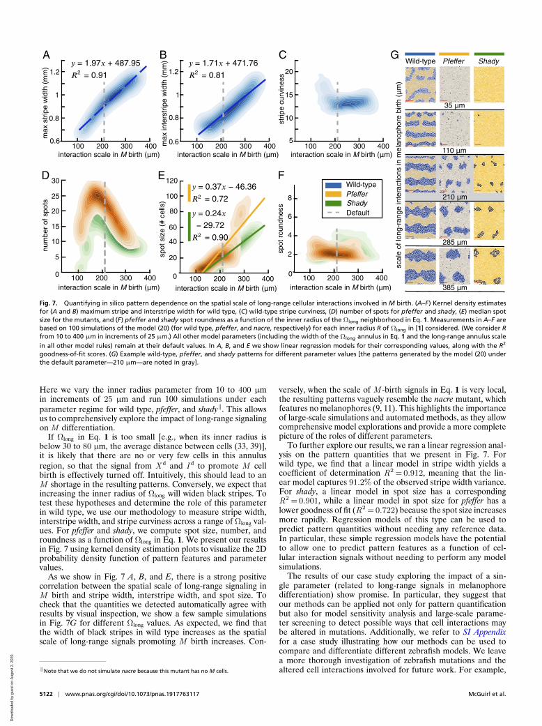
Here we vary the inner radius parameter from 10 to 400 µmin increments of 25 µm and run 100 simulations under eachparameter regime for wild type, pfeffer, and shady‖. This allowsus to comprehensively explore the impact of long-range signalingon M differentiation.

If Ωlong in Eq. 1 is too small [e.g., when its inner radius isbelow 30 to 80 µm, the average distance between cells (33, 39)],it is likely that there are no or very few cells in this annulusregion, so that the signal from X d and I d to promote M cellbirth is effectively turned off. Intuitively, this should lead to anM shortage in the resulting patterns. Conversely, we expect thatincreasing the inner radius of Ωlong will widen black stripes. Totest these hypotheses and determine the role of this parameterin wild type, we use our methodology to measure stripe width,interstripe width, and stripe curviness across a range of Ωlong val-ues. For pfeffer and shady, we compute spot size, number, androundness as a function of Ωlong in Eq. 1. We present our resultsin Fig. 7 using kernel density estimation plots to visualize the 2Dprobability density function of pattern features and parametervalues.

As we show in Fig. 7 A, B, and E, there is a strong positivecorrelation between the spatial scale of long-range signaling inM birth and stripe width, interstripe width, and spot size. Tocheck that the quantities we detected automatically agree withresults by visual inspection, we show a few sample simulationsin Fig. 7G for different Ωlong values. As expected, we find thatthe width of black stripes in wild type increases as the spatialscale of long-range signals promoting M birth increases. Con-

‖Note that we do not simulate nacre because this mutant has no M cells.

versely, when the scale of M -birth signals in Eq. 1 is very local,the resulting patterns vaguely resemble the nacre mutant, whichfeatures no melanophores (9, 11). This highlights the importanceof large-scale simulations and automated methods, as they allowcomprehensive model explorations and provide a more completepicture of the roles of different parameters.

To further explore our results, we ran a linear regression anal-ysis on the pattern quantities that we present in Fig. 7. Forwild type, we find that a linear model in stripe width yields acoefficient of determination R2 = 0.912, meaning that the lin-ear model captures 91.2% of the observed stripe width variance.For shady, a linear model in spot size has a correspondingR2 = 0.901, while a linear model in spot size for pfeffer has alower goodness of fit (R2 = 0.722) because the spot size increasesmore rapidly. Regression models of this type can be used topredict pattern quantities without needing any reference data.In particular, these simple regression models have the potentialto allow one to predict pattern features as a function of cel-lular interaction signals without needing to perform any modelsimulations.

The results of our case study exploring the impact of a sin-gle parameter (related to long-range signals in melanophoredifferentiation) show promise. In particular, they suggest thatour methods can be applied not only for pattern quantificationbut also for model sensitivity analysis and large-scale parame-ter screening to detect possible ways that cell interactions maybe altered in mutations. Additionally, we refer to SI Appendixfor a case study illustrating how our methods can be used tocompare and differentiate different zebrafish models. We leavea more thorough investigation of zebrafish mutations and thealtered cell interactions involved for future work. For example,

5122 | www.pnas.org/cgi/doi/10.1073/pnas.1917763117 McGuirl et al.

Dow

nloa

ded

by g

uest

on

Aug

ust 2

, 202

0

APP

LIED

MA

THEM

ATI

CSD

EVEL

OPM

ENTA

LBI

OLO

GY

the obelix mutant (9) features widened stripes due to unknownaltered cell interactions; by systematically varying parameters inthe model (20) and automatically detecting their impact on stripewidth, one could identify a set of altered cell behaviors that maybe responsible for this phenotype, and these predictions couldthen be evaluated experimentally.

Discussion and ConclusionsOur goal was to provide methods for quantifying agent-basedpatterns across a range of scales. Leveraging topological dataanalysis and machine learning, we developed a methodologythat captures information spanning local features of interactingcells up to macroscopic spots and stripes. Because it describesshape features across a sequence of spatial scales, persistenthomology is a critical tool in our methods. We showed thatcombining this topological tool with clustering methods yieldsa collection of summary statistics that can be automaticallyextracted from patterns using agent coordinates. By reduc-ing the role of visual inspection in describing patterns, ourinterpretable methodology provides a means of analyzing largedatasets and studying how stochasticity in agent interactionsaffects pattern variability. To illustrate the promise of our meth-ods, we applied our methodology to an extensive dataset ofin silico zebrafish skin patterns that we generated using theagent-based model (20). Our methods allowed us to make quan-titative predictions about the types and amounts of variabilitythat may arise in wild-type and mutant zebrafish patterns dueto stochasticity in cellular communication. We used our meth-ods to distinguish and characterize similar mutant patterns, andwe showed how to track pattern features across spatial scalesto study the role of different cellular interactions in patternformation.

Many of our results, which provide a broader view of the agent-based model (20), can be experimentally tested in the future.In particular, after extracting cell coordinates from zebrafishimages, one could compute summary statistics for the empiri-cal data and compare these measurements to our simulations.Our methods could also be applied to other models of zebrafishpatterning, including partial differential equations (e.g., refs. 8and 15–17), stochastic cellular automaton perspectives (17, 18),and agent-based models (e.g., refs. 19 and 21). In the future, onecould use our methods to optimize model parameters or con-duct large screens for cell interactions that may be altered inmutations. Although we focused primarily on analyzing zebrafishpatterns at a fixed point in development, future work could trackpattern features across developmental timelines.

Our approach to quantifying zebrafish patterns begins toaddress major challenges associated with quantifying agent-

based dynamics in an objective and automated way, but thereare also limitations to our methods. First, we make underly-ing assumptions about the patterns that we are studying. As anexample, when we use topological methods to quantify spotsor stripes, we assume that the input patterns have certain fea-tures (e.g., we assume a wild-type input has stripe patterns). Itmay be useful for future studies to automatically classify eachinput pattern as spots or stripes prior to applying the appro-priate pattern quantification methods. Moreover, we focusedprimarily on spots and stripes, but methods for characterizingother patterns [e.g., labyrinth patterns on the choker mutant(11)] could be developed in the future. Finally, we note thatwe built our methodology to take data in the form of agentcoordinates. Empirical images and simulations from partial dif-ferential equation models, however, are continuous functionsdefined over 2D domains. In the former case, one option wouldbe to extract cell locations from image data, and, in the latter,one could apply our methods to cell densities after discretizingspace and applying a density threshold. Fortunately, functionalpersistent homology could avoid both of these extra steps as ittakes function data as its input. In the future, one could applyour approach to continuous-pattern data by replacing the TDAtools that we used with functional persistence throughout ourmethodology.

Although we focused on analyzing pattern variability inzebrafish, we expect that a similar approach can be used toquantify agent-based dynamics in other biological settings. Meth-ods that provide summary statistics for pattern features across arange of length scales open up many possibilities for quantita-tively comparing large datasets of in silico and in vivo patterndata in the future. By working closely with the needs of eachapplication, we expect that our topological perspective can beextended to analyze agent-based dynamics in wound healing,animal flocks, and other forms of collective behavior.

Materials and MethodsData and Code Availability. Implementation details and code are freely avail-able on GitHub: https://github.com/sandstede-lab/Quantifying ZebrafishPatterns. Simulated data are publicly available on Figshare: https://figshare.com/projects/Zebrafish simulation data/72689 (53).

ACKNOWLEDGMENTS. We thank Richard Carthew, William Kath, AnastasiaEskova, Hans Georg Frohnhofer, Uwe Irion, Marco Podobnik, and ChristianeNusslein-Volhard for helpful discussion. M.R.M. is supported by the NationalScience Foundation (NSF) Graduate Research Fellowship Program underGrant 1644760. B.S. is partially supported by the NSF under Grants DMS-1714429 and CCF-1740741. A.V. has been supported by the MathematicalBiosciences Institute and the NSF under Grant DMS-1440386 and is sup-ported by the NSF under Grant DMS-1764421 and the Simons Foundationunder Grant 597491.

1. H. Cho, D. Levy, Modeling the dynamics of heterogeneity of solidtumors in response to chemotherapy. Bull. Math. Biol. 79, 2986–3012(2017).

2. B. D. Cumming, D. L. McElwain, Z. Upton, A mathematical model of wound healingand subsequent scarring. J. R. Soc. Interface 7, 19–34 (2010).

3. Q. Wang et al., A multi-scale model for hair follicles reveals heterogeneousdomains driving rapid spatiotemporal hair growth patterning. eLife 6, e22772(2017).

4. A. P. Singh, C. Nusslein-Volhard, Zebrafish stripes as a model for vertebrate colourpattern formation. Curr. Biol. 25, R81–R92 (2015).

5. M. Watanabe, S. Kondo, Is pigment patterning in fish skin determined by the Turingmechanism? Trends Genet. 31, 88–96 (2015).

6. S. K. McMenamin, M. N. Chandless, D. M. Parichy, Working with zebrafish atpostembryonic stages. Methods Cell Biol. 134, 587–607 (2016).

7. U. Irion, A. P. Singh, C. Nusslein-Volhard, The developmental genetics of vertebratecolor pattern formation: Lessons from zebrafish. Curr. Top. Dev. Biol. 117, 141–169(2016).

8. M. Yamaguchi, E. Yoshimoto, S. Kondo, Pattern regulation in the stripe of zebrafishsuggests an underlying dynamic and autonomous mechanism. Proc. Natl. Acad. Sci.U.S.A. 104, 4790–4793 (2007).

9. F. Maderspacher, C. Nusslein-Volhard, Formation of the adult pigment pattern inzebrafish requires leopard and obelix dependent cell interactions. Development 130,3447–3457 (2003).

10. D. M. Parichy, J. M. Turner, Temporal and cellular requirements for Fms signalingduring zebrafish adult pigment pattern development. Development 130, 817–833(2003).

11. H. G. Frohnhofer, J. Krauss, H. M. Maischein, C. Nusslein-Volhard, Iridophores andtheir interactions with other chromatophores are required for stripe formation inzebrafish. Development 140, 2997–3007 (2013).

12. J. A. Lister, C. P. Robertson, T. Lepage, S. L. Johnson, D. W. Raible, Nacre encodesa zebrafish microphthalmia-related protein that regulates neural-crest-derivedpigment cell fate. Development 126, 3757–3767 (1999).

13. D. M. Parichy, D. G. Ransom, B. Paw, L. I. Zon, S. L. Johnson, An orthologue of the kit-related gene fms is required for development of neural crest-derived xanthophoresand a subpopulation of adult melanocytes in the zebrafish, Danio rerio. Development127, 3031–3044 (2000).

14. S. S. Lopes et al., Leukocyte tyrosine kinase functions in pigment cell development.PLoS Genet. 4, 1–13 (2008).

15. A. Nakamasu, G. Takahashi, A. Kanbe, S. Kondo, Interactions between zebrafish pig-ment cells responsible for the generation of Turing patterns. Proc. Natl. Acad. Sci.U.S.A. 106, 8429–8434 (2009).

16. K. J. Painter, J. M. Bloomfield, J. A. Sherratt, A. Gerisch, A nonlocal model for contactattraction and repulsion in heterogeneous cell populations. Bull. Math. Biol. 77, 1132–1165 (2015).

17. D. Bullara, Y. De Decker, Pigment cell movement is not required for generation ofTuring patterns in zebrafish skin. Nat. Commun. 6, 6971 (2015).

McGuirl et al. PNAS | March 10, 2020 | vol. 117 | no. 10 | 5123

Dow

nloa

ded

by g

uest

on

Aug

ust 2

, 202

0

18. J. Moreira, A. Deutsch, Pigment pattern formation in zebrafish during late larvalstages: A model based on local interactions. Dev. Dyn. 232, 33–42 (2005).

19. A. Volkening, B. Sandstede, Modelling stripe formation in zebrafish: An agent-basedapproach. J. R. Soc. Interface 12, 20150812 (2015).

20. A. Volkening, B. Sandstede, Iridophores as a source of robustness in zebrafish stripesand variability in Danio patterns. Nat. Commun. 9, 3231 (2018).

21. C. E. Caicedo-Carvajal, T. Shinbrot, In silico zebrafish pattern formation. Dev. Biol. 315,397–403 (2008).

22. D. E. Lee, D. R. Cavener, M. L. Bond, Seeing spots: Quantifying mother-offspring sim-ilarity and assessing fitness consequences of coat pattern traits in a wild populationof giraffes (Giraffa camelopardalis). PeerJ 6, e5690 (2018).

23. C. A. Schneider, W. S. Rasband, K. W. Eliceiri, NIH image to ImageJ: 25 years of imageanalysis. Nat. Methods 9, 671–675 (2012).

24. S. Miyazawa, M. Okamoto, S. Kondo, Blending of animal colour patterns byhybridization. Nat. Commun. 1, 66 (2010).

25. I. Djurdjevic, T. Furmanek, S. Miyazawa, S. S. Bajec, Comparative transcriptomeanalysis of trout skin pigment cells. BMC Genom. 20, 359 (2019).

26. H. Hamada et al., Involvement of delta/notch signaling in zebrafish adult pigmentstripe patterning. Development 141, 318–324 (2014).

27. C. M. Topaz, L. Ziegelmeier, T. Halverson, Topological data analysis of biologicalaggregation models. PLoS One 10, 1–26 (2015).

28. M. Hirata, K. Nakamura, S. Kondo, Pigment cell distributions in different tissues ofthe zebrafish, with special reference to the striped pigment pattern. Dev. Dyn. 234,293–300 (2005).

29. S. K. McMenamin et al., Thyroid hormone–dependent adult pigment cell lineage andpattern in zebrafish. Science 345, 1358–1361 (2014).

30. P. Mahalwar, B. Walderich, A. P. Singh, C. Nusslein-Volhard, Local reorganization ofxanthophores fine-tunes and colors the striped pattern of zebrafish. Science 345,1362–1364 (2014).

31. D. M. Parichy, M. R. Elizondo, M. G. Mills, T. N. Gordon, R. E. Engeszer, Normal tableof postembryonic zebrafish development: Staging by externally visible anatomy ofthe living fish. Dev. Dyn. 238, 2975–3015 (2009).

32. L. B. Patterson, D. M. Parichy, Interactions with iridophores and the tissue environ-ment required for patterning melanophores and xanthophores during zebrafishadult pigment stripe formation. PLoS Genet. 9, e1003561 (2013).

33. P. Mahalwar, A. P. Singh, A. Fadeev, C. Nusslein-Volhard, U. Irion, Heterotypic inter-actions regulate cell shape and density during color pattern formation in zebrafish.Biol. Open 5, 1680–1690 (2016).

34. L. B. Patterson, E. J. Bain, D. M. Parichy, Pigment cell interactions and differentialxanthophore recruitment underlying zebrafish stripe reiteration and Danio patternevolution. Nat. Commun. 5, 5299 (2014).

35. M. Inaba, H. Yamanaka, S. Kondo, Pigment pattern formation by contact-dependentdepolarization. Science 335, 677 (2012).

36. D. S. Eom, E. J. Bain, L. B. Patterson, M. E. Grout, D. M. Parichy, Long-distance com-munication by specialized cellular projections during pigment pattern developmentand evolution. eLife 4, e12401 (2015).

37. A. Fadeev, J. Krauss, A. P. Singh, C. Nusslein-Volhard, Zebrafish leucocyte tyrosinekinase controls iridophore establishment, proliferation and survival. Pigment CellMelanoma Res. 29, 284–296 (2016).

38. A. P. Singh, U. Schach, C. Nusslein-Volhard, Proliferation, dispersal and patternedaggregation of iridophores in the skin prefigure striped colouration of zebrafish. Nat.Cell Biol. 16, 604–611 (2014).

39. G. Takahashi, S. Kondo, Melanophores in the stripes of adult zebrafish do not havethe nature to gather, but disperse when they have the space to move. Pigment CellMelanoma Res. 21, 677–686 (2008).

40. H. Yamanaka, S. Kondo, In vitro analysis suggests that difference in cell movementduring direct interaction can generate various pigment patterns in vivo. Proc. Natl.Acad. Sci. U.S.A. 111, 1867–1872 (2014).

41. D. M. Parichy, J. M Turner, Zebrafish puma mutant decouples pigment pattern andsomatic metamorphosis. Dev. Biol. 256, 242–257 (2003).

42. B. Walderich, A. P. Singh, P. Mahalwar, C. Nusslein-Volhard, Homotypic cell com-petition regulates proliferation and tiling of zebrafish pigment cells during colourpattern formation. Nat. Commun. 7, 11462 (2016).

43. G. Carlsson, Topology and data. Bull. Am. Math. Soc. 46, 255–308 (2009).44. F. Chazal, V. de Silva, M. Glisse, S. Oudot, The Structure and Stability of Persistence

Modules (Springer International Publishing, ed. 1.0, 2016).45. H. Edelsbrunner, J. L. Harer, Computational Topology, an Introduction (American

Mathematical Society, 2010).46. R. Ghrist, Elementary Applied Topology (Createspace, ed. 1.0, 2014).47. A. Zomorodian, Topology for Computing (Cambridge University Press, 2009).48. C. M. Bishop, Pattern Recognition and Machine Learning (Springer Science+Business,

New York, NY, 2006).49. T. Hastie, R. Tibshirani, J. Friedman, The Elements of Statistical Learning (Springer,

2009).50. K. Howe et al., The zebrafish reference genome sequence and its relationship to the

human genome. Nature 496, 498–503 (2013).51. E. H. Budi, L. B. Patterson, D. M. Parichy, Post-embryonic nerve-associated precursors

to adult pigment cells: Genetic requirements and dynamics of morphogenesis anddifferentiation. PLoS Genet. 7, e1002044 (2011).

52. C. M. Dooley, A. Mongera, B. Walderich, C. Nusslein-Volhard, On the embry-onic origin of adult melanophores: The role of ErbB and Kit signalling inestablishing melanophore stem cells in zebrafish. Development 140, 1003–1013(2013).

53. M. R. McGuirl, A. Volkening, B. Sandstede, Zebrafish Simulation Data (2020).https://figshare.com/projects/Zebrafish simulation data/72689. Deposited 10 January2020.

5124 | www.pnas.org/cgi/doi/10.1073/pnas.1917763117 McGuirl et al.

Dow

nloa

ded

by g

uest

on

Aug

ust 2

, 202

0