REVIEW

Topographic ERP Analyses: A Step-by-Step Tutorial Review

Micah M. Murray Æ Denis Brunet Æ Christoph M. Michel

Accepted: 13 February 2008 / Published online: 18 March 2008! Springer Science+Business Media, LLC 2008

Abstract In this tutorial review, we detail both therationale for as well as the implementation of a set of

analyses of surface-recorded event-related potentials

(ERPs) that uses the reference-free spatial (i.e. topo-graphic) information available from high-density electrode

montages to render statistical information concerning

modulations in response strength, latency, and topographyboth between and within experimental conditions. In these

and other ways these topographic analysis methods allow

the experimenter to glean additional information and neu-rophysiologic interpretability beyond what is available

from canonical waveform analyses. In this tutorial we

present the example of somatosensory evoked potentials(SEPs) in response to stimulation of each hand to illustrate

these points. For each step of these analyses, we provide

the reader with both a conceptual and mathematicaldescription of how the analysis is carried out, what it

yields, and how to interpret its statistical outcome. We

show that these topographic analysis methods are intuitiveand easy-to-use approaches that can remove much of the

guesswork often confronting ERP researchers and also

assist in identifying the information contained within high-density ERP datasets.

Keywords Electroencephalography (EEG) !Event-related potentials (ERPs) ! Topography ! Spatial !Reference electrode ! Global field power !Global dissimilarity ! Microstate segmentation

Introduction

This tutorial review has been predicated by a growing

interest in the use of EEG and ERPs as a neuroimagingtechnique capable of providing the experimenter not only

with information regarding when experimental conditionsdiffer, but also how conditions differ in terms of likely

underlying neurophysiologic mechanisms. There is an

increasing appreciation of the fact that EEG and ERPscomport information beyond simply the time course of

brain responses or ‘‘components’’ that correlate with a

psychological/psychophysical parameter. They can identifyand differentiate modulations in the strength of responses,

modulations in the latency of responses, modulations in the

underlying sources of responses (vis a vis topographicmodulations), as well as combinations of these effects.

Moreover, this information is attainable with sub-milli-

second temporal resolution. Our focus here is on providinga tutorial for how to extract such information with minimal

experimenter bias and to test such information statistically.

M. M. Murray (&) ! D. Brunet ! C. M. MichelElectroencephalography Brain Mapping Core, Center forBiomedical Imaging of Lausanne and Geneva, RadiologieCHUV BH08.078, Bugnon 46, Lausanne, Switzerlande-mail: micah.murray@chuv.ch

M. M. MurrayThe Functional Electrical Neuroimaging Laboratory,Neuropsychology and Neurorehabilitation Service, VaudoisUniversity Hospital Center and University of Lausanne,46 rue du Bugnon, 1011 Lausanne, Switzerland

M. M. MurrayThe Functional Electrical Neuroimaging Laboratory, RadiologyService, Vaudois University Hospital Center and University ofLausanne, 46 rue du Bugnon, 1011 Lausanne, Switzerland

D. Brunet ! C. M. MichelFunctional Brain Mapping Laboratory, Department ofFundamental and Clinical Neuroscience, University Hospital andUniversity Medical School, 24 Rue Micheli du Crest,1211 Geneva, Switzerland

123

Brain Topogr (2008) 20:249–264

DOI 10.1007/s10548-008-0054-5

Researchers using EEG/ERPs might find themselves

daunted by the shear quantity of data that is now routinelyacquired (e.g. 64–256 channels and amplifiers that digitize

data simultaneously from all channels at rates from 500 Hz

upwards) and perhaps also by the myriad names of ERPcomponents appearing in the literature (e.g. [33] for a

recent overview). In the case of a 64-channel ERP inves-

tigation with epochs spanning 100 ms pre-stimulus to900 ms post-stimulus at 500 Hz digitalization, there would

be a data matrix containing 32,000 values (which could befurther expanded if examined in terms of its spectral

decomposition). If one were to assume complete indepen-

dence of the measurements as a function of time and space/electrode (which is not the case and thus makes this issue

all the more problematic because simple Bonferroni cor-

rection is inadequate; e.g. [20] for discussion), then bystochastic processes alone 160 of these 32,000 values

would meet the 0.05 criterion of statistical significance if

the experimenter were to compare all of these data fromthe two experimental conditions. Bearing this in mind, how

then should the experimenter choose which of the data to

analyze, given the necessity for data reduction in EEG/ERPresearch, while also avoiding the possibility that the data

they analyze are among the 160 values that significantly

differ by chance? It should be mentioned that this is not aproblem unique to EEG/ERPs. Researchers working with

fMRI datasets must also confront this and related issues,

which have been most notably addressed by the authors ofStatistical Parametric Mapping (SPM; [13]; http://www.

fil.ion.ucl.ac.uk/spm). A prevailing and even recommended

approach in EEG/ERP research has been for the experi-menter to a priori select time periods or components of

interest (often based on hypotheses generated from prior

studies) as recorded at a chosen subset of electrodes (e.g.[22, 33]). For example, in a set of published guidelines for

conducting ERP research [53, p. 141] proposed that ‘‘the

simplest approach is to consider the ERP waveform as a setof waves, to pick the peaks (and troughs) of these weaves,

and to measure the amplitude and latency at these deflec-

tions.’’ Aside from the experimenter bias inherent to thisapproach, there are several additional weaknesses of ana-

lyzing ERP voltage waveforms that render the results

arbitrary and of severely limited (neurophysiologic) inter-pretability. For example, an a priori focus on one or a few

components of interest leads to the possibility that other

(earlier) time periods and effects are overlooked, such asduring periods of low-amplitude in a given waveform (e.g.

[54, 55]). The spatio-temporal analysis methods that we

summarize here can render a far more complete andinformative interpretability without any a priori bias on

certain time periods or scalp locations. Such is not to

suggest that these methods cannot be incorporated withpurely hypothesis-driven research. In the case of emotion

processing, for example, the experimenter may be testing

the hypothesis that negative emotional stimuli are pro-cessed more quickly and via a more efficient neural circuit

(i.e. different generators) than positive or neutral stimuli.

As will be shown below, canonical analyses of voltagewaveforms present serious pitfalls and limitations when

addressing such questions/hypotheses.

We would be remiss to not immediately acknowledgeseveral prior works that have either introduced or over-

viewed many of the methods/issues we shall describe here.Most important among these is the seminal works of Dietrich

Lehmann and his scholars (e.g. [3, 27, 31, 32, 37, 38, 60, 61),

though several others are also noteworthy [11, 12, 15].We have organized this tutorial in the following way.

First, we discuss the limitations and pitfalls of canonical

waveform analyses, providing some concrete examples.Afterwards we detail the procedures for each step of elec-

trical neuroimaging. In each section, we have attempted to

introduce the theoretical basis of and to explain in simpleterms and with mathematically simple examples how topo-

graphic analyses can be conducted, what information they

yield, and how this information can be statistically analyzedand interpreted. While this tutorial discusses the case of

somatosensory evoked potentials in order to give the reader

an intuitive example based on known underlying neuro-physiology, the methods presented here can be readily

applied to issues in emotion research and cognitive neuro-

science in general (see [55] for an example as well as studiescited throughout this tutorial for applications to specific

questions in sensory-cognitive processing). Topographic

mapping of the EEG end ERP is often a precursor to sourcelocalization. It is therefore of crucial importance that the

topography of the scalp electric field is properly analyzed

and interpreted before attempting to localize the underlyingbrain sources. This review focuses on the analysis of the

topography of the scalp electric field. Readers interested in a

more in-depth coverage of the issue of source localization arereferred to [2, 23, 40]. All analyses presented in this tutorial

have been conducted using CarTool software (http://

brainmapping.unige.ch/cartool.htm).

Data for this Tutorial

The data we use here to illustrate the electrical neuro-

imaging analyses are a subset from a previouslypublished study demonstrating partially segregated func-

tional pathways within the somatosensory system [6], and

full details concerning the paradigm and data acquisitioncan be found therein. We provide only the essential

details here.

Continuous EEG was acquired from six healthy partic-ipants at 512 Hz though a 128-channel Biosemi ActiveTwo

250 Brain Topogr (2008) 20:249–264

123

AD-box (http://www.biosemi.com) referenced to the

common mode sense (CMS; active electrode) and groun-ded to a passive electrode. Peri-stimulus epochs of EEG

(-96 ms pre-stimulus to 488 ms post-stimulus onset) were

averaged separately for stimulation of the left and righthand and for each participant. For the present tutorial only

non-target, distracter trials from the ‘‘what’’ condition were

included (c.f. Table 1 of [6]). In addition to a ±100lVartifact rejection criterion, EEG epochs containing eye

blinks or other noise transients were excluded. Prior togroup-averaging, data at artifact electrodes from each

subject were interpolated using a spherical spline interpo-

lation [52]. Likewise, data were baseline corrected, usingthe pre-stimulus period, and band-pass filtered (0.68–

40.0 Hz).

Tactile stimuli were square wave pulses (300 ms dura-tion; 44,100 Hz sampling) presented through Oticon bone

conduction vibrators (Oticon Inc., Somerset, NJ) with

1.6 cm 9 2.4 cm surfaces. Two spatial positions (one inthe left hemispace and one in the right hemispace) and two

vibration frequencies (22.5 and 110 Hz) were used. Stim-

ulus delivery and behavioral response recording wascontrolled by E-prime (Psychology Software Tools, Inc.,

Pittsburgh, PA; http://www.pstnet.com/eprime).

As will become clear below, the specific data we used

are not particularly crucial for the points and methods wewish to illustrate here. The utility of comparing SEPs to left

and right hand stimulation is that this is an intuitive

example with clear neurophysiologic underpinnings interms of known somatotopic cortical organization.

Waveform Analyses: Limitations and Pitfalls

The core limitation (and pitfall) of analyzing voltage ERP

waveforms is that they are reference-dependent. Although

there is a long history of viewpoints concerning the ‘best’or ‘appropriate’ reference (e.g. [8, 9, 48], see also [40] for a

more recent discussion that includes the role of the refer-

ence in source estimations), it will always remain a choiceand therefore a source of bias introduced by the experi-

menter. More important is the fact that this choice will

critically impact the (statistical) outcome the experimenterobserves when analyzing waveform measurements and by

extension the interpretation of the data. This section

therefore illustrates precisely these points.Figure 1 displays group-averaged ERPs (s.e.m. indi-

cated) to vibrotactile stimulation of the left and right hand

Table 1 Some dependent measures obtainable from the ‘fitting’ procedure and their interpretability

Dependent measure What’s actually being quantified Interpretation of a map9 condition interaction

Considerations & caveats

Number of data pointslabeled with a giventemplate map (a.k.a.frequency of mappresence or map duration)

For each subject, the number of datapoints, over a specified timeperiod, when a template mapyields the highest spatialcorrelation value over othertemplate maps

Different template maps bestrepresent the experimentalconditions. When appropriate,post-hoc contrasts should beconducted

A higher spatial correlation doesforcibly not translate into asignificantly higher spatialcorrelation (see below). Forexample, although 96% is higherthan 95%, it does not mean thatthese values significantly differ.Results of the TANOVA analysiscan help address this issue

GEV of a given templatemap

For each subject, the GEV over aspecific time period of a giventemplate map for a givencondition (see Appendix I forformula)

Different template maps better‘‘explain’’ each condition

When this analysis is conductedunder competitive fittingconditions (i.e. different maps arevying for labeling of the sametime point), a given map might notalways label the data from eachsubject and condition. In this case,missing values should beappropriately handled in thestatistical analysis

First onset/last offset of agiven template map

The time point in each subject’s datafrom a given condition when agiven template map yields thehighest spatial correlation(relative to other template mapsbeing fit) for the first/last timeover a specified time period

A latency shift and/or durationdifference between conditions intheir components or functionalmicrostates, as identified bydifferent template maps

There is no a priori restriction onwhether or not the template maponsets and remains thepreferentially fit map. That is,only the first onset and last offsetare quantified, rather than whetheror not there were multiple onsetsand offsets over a given timeperiod

Brain Topogr (2008) 20:249–264 251

123

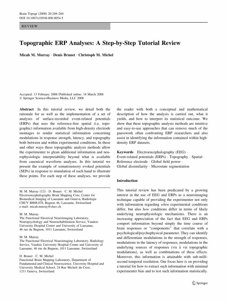
(blue and red traces, respectively) as recorded from elec-

trodes at scalp locations C5 and C6, using standard

electrode position nomenclature [46]. More specifically,panels a–c of this figure display the ERPs when different

reference channels are selected (average reference, T7

reference (to emulate the left mastoid/earlobe), and T8reference (to emulate the right mastoid/earlobe), respec-

tively). The reader should note several points from this

figure. First, the shape of the ERP waveforms changes withdifferent reference electrodes. A given peak/trough might

appear or disappear. Second, the variance around the ERP

(and by extension the s.e.m.) changes with different ref-

erence electrodes. Third, the latency and electrode(s) at

which significant differences are obtained between condi-tions changes with different reference electrodes.

In Fig. 1a, differences between ERPs to left-hand and

right-hand stimuli are observed at both electrodes C5 andC6 beginning at *40 ms. One might interpret this as a

bilateral and approximately equi-opposite effect with larger

responses to left-hand stimuli at electrode C6 and to right-hand stimuli at electrode C5. From such, one might further

conclude that each hemisphere responds in opposite ways

Fig. 1 The effect of thereference electrode. Group-averaged ERP waveforms aredisplayed in response to left-hand and right-handsomatosensory stimulation (blueand red traces, respectively).Cyan and pink traces indicatethe s.e.m. for these group-average ERPs. Panels a–c depictthe ERPs as measured fromelectrodes C5 and C6 whendifferent reference locations areused. The reader should note thechange in waveform shape, inthe magnitude of the measureds.e.m., and in the presence/absence of differences betweenconditions. The right-hand sideof the figure depicts the voltagetopography of these data at55 ms post-stimulus onset. Thereader should note that althoughthe color value ascribed to agiven location changes with thechoice of the reference(indicated by the projected axisand equator), the form of thetopography is reference-independent

252 Brain Topogr (2008) 20:249–264

123

to stimulation of each hand. In Fig. 1b, with T7 as refer-

ence, such differences are observed only at electrode C6.One might interpret this as a right-lateralized effect with no

evidence for response differences at electrodes over the left

hemiscalp. From such, one might conclude that only theright hemisphere responses to tactile stimuli of the hands.

Finally, in Fig. 1c, with T8 as reference, differences are

observed only at electrode C5. One might interpret this as aleft-lateralized effect with no evidence for response dif-

ferences at electrodes over the right hemiscalp. From such,one might conclude that only the left hemisphere responses

to tactile stimuli of the hands.

Which of the patterns of results shown in Fig. 1 andtheir subsequent interpretations is ‘correct’? While all are

equally ‘correct’ from a statistical perspective, where and

when responses to left-hand and right-hand stimulation aredifferentially processed cannot be unequivocally addres-

sed by the above analyses of ERP waveforms, as the very

presence of a given component in an ERP waveform aswell as its modulation across experimental conditions is

entirely reference-dependent. While the above example

shows the data for the average reference and emulationsof lateralized references to clearly illustrate our point, the

caveats we describe apply to any reference location

(vertex, nose, etc.). Even if it is ‘‘customary’’ for a givenERP community or lab to use one reference over another,

the abovementioned analytical and interpretational pit-

falls will remain present. That is, the obtained waveformshape and statistical result only apply for that chosen

reference.

A related issue with canonical analyses of voltage wave-forms concerns the interpretation of condition 9 electrode

interactions observed in an analysis of variance (ANOVA).

This issue has been extensively treated by McCarthy andWood [36] who rightly pointed out how this analysis cannot

differentiate modulations in topography from modulations in

amplitude when data are not first scaled. In particular, theypresented three distinct scaling methods. One involves iden-

tifying the instantaneous maximum and minimum for each

condition and subtracting the minimum value as well as thedifference between the maximum and minimum from each

electrode. A second involves scaling by a pre-defined value

(see [24]); the shortcomings of which are detailed in [36]. Thethird,which they (andwe) favor, involves dividing thevalue at

each electrode by the instantaneous global field power (GFP;

see below); a procedure that they refer to asvector scaling.Themethods proposed byMcCarthy and Wood [36] are routinely

referred to and often applied/recommended [53]. As such, it is

worthwhile to mention some important caveats with how thismethod has been applied (see also [10]). The first is that

McCarthy and Wood’s [36] approach is only valid when the

data from the entire electrode montage is included in theANOVA; a practice nowadays rarely performed. A second,

intertwined and inescapable caveat is that ANOVAs based on

data from voltage waveforms will always be reference-dependent even when scaled. We return to the issue of sta-

tistically identifying topographic modulations in a reference-

independent manner, below.From this example the reader should gain a sense of the

severe limitations and pitfalls of analyzing ERP voltage

waveforms. We have provided the example of somato-sensory processing, but this could readily be extrapolated

to more cognitive functions such as attention, language,and emotion, as well as the components typically ascribed

to them. For some, this ‘‘reference-dependent’’ attribute

has been viewed as the principal shortcoming of EEGversus magnetoencephalography (MEG; [50, 69, 70]).

However, as will be shown throughout this tutorial and

elsewhere in this special issue [55], alternative and easy-to-use analyses can be performed on EEG/ERP data (as well

as MEG/MEF data) that do allow researchers to address

fundamental neurophysiologic questions.The first step for making EEG/ERP analyses more

informative is to identify a reference-independent measure.

We would direct the reader to the right-sided portion ofFig. 1 where the voltage topography at 55 ms post-stimu-

lus onset is shown in response to stimulation of the left

hand and right hand (blue and red frames, respectively).The projected axis and equator indicate the 0 lV plane (i.e.

the reference). As before, the reader should note several

points by comparing topographies when different referencechannels are used. First, changing the reference shifts

vertically the position of the 0 lV plane. Second and of far

greater importance, the shape of the topography remainsconstant even though the color ascribed to a given position

changes (see also Fig. 3 in [40]). That is, the configuration

of the electric field at the scalp (i.e. the topographic map) isreference-independent [14, 31]. To provide the reader with

a more everyday example, the shape of a mountain range

remains constant even if the altitude of sea level (i.e. thereference elevation) were to change [31]. A third point that

should be taken from this figure is that the topographies of

responses to left-hand and right-hand stimuli sharply differand differ in a reference-independent manner. As will be

shown below, the extent of topographic similarity or dis-

similarity can be quantified and statistically tested. Of moreimportance is the fact that topographic differences have

direct neurophysiologic interpretability. Changes in the

topography of the electric field at the scalp can only becaused by changes in the configuration of the underlying

intracranial sources (given the exclusion of artifacts such as

eye movements, muscle activity, etc.), though the converseneed not be the case [12, 31, 67].

We would be remiss not to mention that in an effort to

obtain reference-free waveforms some have advocated theanalysis of so-called current source density (CSD) or

Brain Topogr (2008) 20:249–264 253

123

Laplacian waveforms1 over their voltage counterparts (e.g.

[41, 45, 59, 68). This procedure is undoubtedly beneficial inthat it indeed eliminates the reference-dependent problem

inherent to voltage waveforms (as well as contributions of

volume conduction within the plane of the scalp) and is asuitable alternative for those researchersmore accustomed to

handling waveform data. However, CSD waveforms con-

sidered in isolation do not in and of themselves provideinformation concerning the underlying neurophysiologic

mechanism(s) giving rise to a modulation between experi-mental conditions. In addition, the CSD is not readily

calculated at the border of the electrode montage, and the

CSD is generally more sensitive to the level of noise in thedata. Finally, the experimenter would still be faced with

the choice of which CSD waveforms and time periods to

analyze.

Why We Use the Average Reference

In the above we have highlighted the caveats of reference-

dependent measurements. However, EEG/ERP requires theuse of a reference. So, which one should be used? We

advocate the use of a common average reference [32] for

the following reason. Inverse solution methods (i.e. meth-ods to reconstruct the intracranial sources of surface-

recorded data) recalculate the data to a common average

reference. This is because of the biophysical assumption ofquasi-stationarity—i.e. that the net source activity at each

instant in time within the brain sums to zero. Because the

reference electrode adds a constant potential value to thevalue recorded at each electrode and instant in time, a

‘‘re-centering’’ of the data (i.e. a removal of this constant

value) is necessary before applying an inverse solution soas to avoid violating the above quasi-stationarity assump-

tion. Mathematically, this is equivalent to calculating the

average reference of the surface-recorded EEG/ERP [48].When using the average reference, it is therefore

important to have adequate sampling of the electric field at

the scalp. Discussions of how many electrodes andappropriate inter-electrode distances are outside the scope

of this tutorial review (see e.g. [30, 65] for treatments of

this issue). However, the relatively low cost of EEGequipment makes high-density montages accessible to

most laboratories. Another important issue when using the

average reference, performing the analyses detailed here,

and estimating intracranial sources, is how to cope withartifact-contaminated channels. This applies to both the

single-subject and group-averaged data. Values at such

channels are typically interpolated (see [40] for discussionfor different methods). Likewise, group-averaged data

require normalization to the same electrode configuration/

positions before averaging [53].It is also worthwhile to mention a common misunder-

standing in how the average reference should be computed.Under typical experimental conditions, the recording ref-

erence is often discarded. However, the data at this location

(provided it is near the brain and not elsewhere on the bodysurface or even off the body) is nevertheless a valid sam-

pled value of the brain’s electric field at that location and as

such should be included in the electrode montage and dataanalyses, being ascribed a value of 0 lV as a function of

time in all the formulae, including in the calculation of the

average reference (see Appendix I).2 Once the data havebeen recalculated to the average-reference, the reference

electrode is just another electrode within the montage with

a measurement of potential varying as a function of time(see topographic representations in Fig. 1).

Global Field Power: A Single, Reference-IndependentMeasure of Response Strength

We now return to the kinds of neurophysiologic informa-

tion we wish to extract from the EEG/ERP data, beginning

with response strength. In the above, we detailed the pit-falls and limitations of analyzing ERP voltage waveforms

due to their being dependent on the choice of the refer-

ence electrode(s). Global Field Power (GFP), by contrast,constitutes a single, reference-independent measure of

response strength. GFP was first introduced by Lehmann

and Skrandies [32] and has since become a commonplacemeasure among MEG users. Mathematically, GFP equals

the root mean square (RMS) across the average-referenced

electrode values at a given instant in time. More simply,

1 For readers less familiar with CSD derivations, it is perhapsworthwhile to briefly describe what is being calculated that makesthem reference-independent. The CSD or Laplacian derivationinvolves calculating the 2nd spatial derivative across the electrodemontage (i.e. the degree of change of the degree of change in thevoltage measured at electrode X relative to its neighbors). In this way,CSD derivations are intrinsically based on spatial gradients in theelectric field at the scalp.

2 Including the reference in the average reference calculation is verymuch desired, but becomes problematic if the reference has beenplaced far away from the brain. In some montages, a nose reference isalready somewhat problematic because its inclusion in the averagereference calculation will add an extreme point without anysurrounding electrodes. In such cases, the experimenter might preferto take it out of the montage and calculate the average reference fromthe remaining electrodes, particularly when a small number ofelectrodes are used. The reason is that the influence of the one‘‘unknown’’ value (i.e. the reference) on the other known values is1/(# of electrodes). Of more critical importance is that the referenceitself is not artifact-contaminated (e.g. eye movements, cardiacactivity, etc.).

254 Brain Topogr (2008) 20:249–264

123

GFP is the standard deviation of all electrodes at a given

time (see Appendix I). In the case of ERPs, the resultantGFP waveform is a measure of potential (lV) as a functionof time. GFP can be assessed statistically using approaches

common to ERP research (e.g. time point by time point;area measures, peak measures, etc.). It is important to

recall, however, that because GFP is a non-linear trans-

formation, the GFP of the group-average ERP is notequivalent to the mean GFP of the single-subject ERPs.

Thus, experimenters should exercise caution when visuallyinspecting and/or displaying GFP waveforms for group-

averaged data.

What GFP tells the researcher is on average across theelectrode montage how strong a potential is being recorded.

What GFP does not tell the researcher is any information

about how this potential is distributed across the electrodemontage—i.e. where large and small potentials were

measured. These points are illustrated in Fig. 2, which

displays four hypothetical data matrices (i.e. the potentialvalues recorded from 12 electrodes at a given latency). The

four conditions differ in the follow ways. Condition 2 is

precisely twice that of Condition 1 at each electrode,resulting in an identical spatial distribution of values that

are simply stronger in Condition 2. Condition 3 is the

mathematical inverse of Condition 1 (i.e. the value at eachelectrode was multiplied by -1), thereby resulting in a

different spatial distribution (i.e. topography) of the same

values (i.e. the frequency of each value/color is identical).Note that Condition 3 is included to illustrate an extreme

case that is unlikely under typical experimental conditions.

Condition 4, by contrast, represents a more typical obser-vation in that it varies in both strength and topography from

Condition 1. Figure 2b displays the squared value of these

potentials at each electrode, the sum of these values acrosselectrodes, and the resultant GFP. Note that while Condi-

tions 1/3 have the same GFP and Conditions 2/4 have the

same GFP, Conditions 1/3 have a GFP half that of Con-ditions 2/4. As such, it is important to note that the

observation of a GFP modulation does not exclude the

possibility of a contemporaneous change in the electricfield topography. Nor does it rule out the possibility of

topographic modulations that nonetheless yield statistically

indistinguishable GFP values. For example, in the case ofthe somatosensory ERPs presented above, there is no evi-

dence of a reliable GFP difference between responses to

left-hand and right-hand stimulation (Fig. 3a). However,we should add that the observation of a GFP modulation in

the absence of a topographic modulation would most par-

simoniously be interpreted as a modulation of the numberof synchronously activated but statistically indistinguish-

able generators across experimental conditions [62]. Next,

we present methods for identifying and quantifying topo-graphic modulations.

Global Dissimilarity: A Single, Strength-IndependentMeasure of Response Topography

Global dissimilarity (DISS) is an index of configuration

differences between two electric fields, independent of theirstrength. Like GFP, DISS was first introduced by Lehmann

and Skrandies [32]. This parameter equals the square root of

the mean of the squared differences between the potentialsmeasured at each electrode (versus the average reference),

each of which is first scaled to unitary strength by dividing

by the instantaneous GFP (see Appendix I). To provide aclearer sense of the calculation of DISS, consider again the

data in Fig. 2. As already mentioned in the above section,

Conditions 1 and 2 have the same topography but differentstrengths, whereas Conditions 1 and 3 have the same

strength but different (inverted) topographies. Finally Con-

ditions 1 and 4 differ in both their strength and topography.Figure 2a shows the original data, whereas the data in

Fig. 2c have been GFP-normalized. Having thus re-scaled

all four conditions to have the same GFP, the topographicsimilarities and differences between conditions becomes

readily apparent. As shown in Fig. 2d, DISS can range from

0 to 2, where 0 indicates topographic homogeneity and 2indicates topographic inversion.

Unlike GFP, however, the statistical analysis of DISS is

not as straightforward, in part because DISS is a singlemeasure of the distance between two vectors (each of which

represents one electric field topography), rather than aseparate measure for each condition about which a mean

and variance can be calculated. Consequently, a non-para-

metric statistical test has to be conducted, wherein thedependent measure is the DISS between two maps at a

given point in time, t. We and others have colloquially

referred to this analysis as topographic ANOVA orTANOVA (e.g. [6, 7, 42, 44, 54, 63, 71], see also [29]),

though we would immediately remind the reader that no

analysis of variance is being conducted. Instead, TANOVAentails a non-parametric randomization test [34].3 To do

this for a within-subjects design, an empirical distribution

of possible DISS values is determined by (1) re-assigningsingle-subject maps to different experimental conditions at

a within-subject level (i.e. permutations of the data), (2)

recalculating the group-average ERPs, and (3) recalculatingthe resulting DISS value for these ‘new’ group-average

ERPs. The number of permutations that can be made with a

group-average ERP based on n participants is 2n, though

3 Other methods for determining whether two electric fields differhave been proposed [25, 36, 64, 65]), criticized [21], and defended[58]. Some of these methods use average referenced and/or normal-ized values (like the Tsum2), but not all, which disqualifies them astrue topographic analyses. Also, note the impossibility of using theHotelling T2 multivariate statistic, as it requires more samples thanelectrodes and it precludes the use of the average reference.

Brain Topogr (2008) 20:249–264 255

123

Fig. 2 Measurement of GFP and DISS. The basis for the reference-independent measurement of response strength and topography isshown. Color values throughout this figure denote polarity, withwarmer colors indicating positive values and cooler colors negativevalues. (a) Hypothetical data from four different conditions from anarray of 12 electrodes. The reader should note that Condition 2 isprecisely twice the value of Condition 1 at each electrode and thatCondition 3 is the inverse of the values of Condition 1 (i.e. the valueat each electrode has been multiplied by -1). Finally, Condition 4 is aspatial re-arrangement of the values of Condition 2, making it differin both strength and topography from Condition 1. (b) The squaredvalue at each electrode and the summed value across electrodes as

well as the resulting GFP. The reader should note that Conditions 1and 3 have the same GFP, even though their topographies areinverted, and that Conditions 2/4 have twice the GFP of Conditions1/3. (c) The GFP-normalized values of the original data displayed inpanel a. The reader should note that once strength differences arenormalized, Conditions 1 and 2 have the same topography, whereasthe topography of Condition 3 is the inversion of Conditions 1 and 2(i.e. the extreme case) and the topography of condition 4 is slightlydifferent from that of the other conditions. (d) The squared differenceof the values in panel c at each electrode as well as the resulting DISS.The reader should note that DISS ranges from 0 to 2, with the formerindicating identical topographies and the latter inverted topographies

256 Brain Topogr (2008) 20:249–264

123

Manly [34] suggests that 1,000–5,000 permutations is suf-

ficient. The DISS value from the actual group-average ERPsis then compared with the values from the empirical dis-

tribution to determine the likelihood that the empirical

distribution has a value higher than the DISS from the actualgroup-average ERPs. This procedure can then be repeated

for each time point. The results of this analysis for the

somatosensory ERPs presented above is shown in Fig. 3b,which displays the occurrence of significant topographic

differences between responses to left-hand and right-hand

stimuli initially over the *40–70 ms post-stimulus period

(as well as at subsequent time periods). For a between-

subjects design, the analysis is generally identical, exceptthat the permutations are performed by first putting all

participants’ data into one pool irrespective of experimental

condition/group. Then new conditions/groups are randomlydrawn and group-average ERPs are calculated for deter-

mining the empirical distribution.

At a neurophysiologic level, because electric field chan-ges are indicative of changes in the underlying generator

configuration (e.g. [12, 31, 67]) this test provides a statisticalmeans of determining if and when the brain networks acti-

vated by the two conditions differ. In this way, the reader

should note how response strength (GFP) and responsetopography (DISS) can be measured and analyzed orthogo-

nally and in a completely reference-independent manner

without the necessity of a priori selecting time periods orelectrodes for analyses. Moreover, these two attributes can

(and in our view should always) be analyzed as a function oftime without the necessity of the experimenter a priorichoosing time periods or components of interest. Still, some

considerations when interpreting results of analyses with

DISS are worth mentioning. Primary among these is thatalthough a significant effect is unequivocal evidence that the

topographies (and by extension configuration of intracranial

generators) differ, this analysis does not in and of itself dif-ferentiate between several alternative underlying causes. For

example, a significant difference may stem from one con-

dition having one single and stable ERP topography during agiven time period and the other condition another single and

stable ERP topography over the same time period. That is,

representing the electric field topography at a given timepoint by a letter, one condition might read ‘‘AAAAAA’’ and

the other ‘‘BBBBBB’’. Alternatively, each condition may be

described by either single or multiple stable ERP topogra-phies over the same time period (i.e. ‘‘AAABBB’’ versus

‘‘CCCDDD’’ or ‘‘AAAAAA’’ versus ‘‘BBCCDD’’. Topo-

graphic differences might likewise stem from a latency shiftbetween conditions (‘‘ABCDEF’’ versus ‘‘BCDEFG’’).

Because all of these alternatives could result in highly similar

(if not identical) patterns of statistical outcomes, additionalanalyses have been devised to determine the pattern of

topographies both within and between conditions.

Topographic Pattern Analysis & Single-Subject‘‘Fitting’’

An important issue, parallel to those already outlined above,

in the analysis of EEG/ERPs is how to define the temporalintervals of a component, the temporal intervals for statisti-

cal analyses, and the temporal intervals to subject to source

estimation. This becomes increasingly challenging when

Fig. 3 Results of applying the methods of this tutorial to somato-sensory ERPs. (a) The results of the analysis of GFP across time,which was based on the variance across subjects. This analysis failedto reveal any differences between responses to stimulation of eachhand. (b) The results of the TANOVA analysis. ERPs to stimulationof each hand first topographically differed over the *40–70 ms post-stimulus period. (c) The results of the fitting after having conducted atopographic pattern analysis based on AAHC (see text for details).Template maps are displayed for the 40–70 ms period. The bar graphshows that one template map better represents responses to left-handstimulation and another template map better represents responses toright-hand stimulation

Brain Topogr (2008) 20:249–264 257

123

high-density electrode montages are used. Also, the

approach of averaging the measured potentials over a fixedand/or experimenter-defined time interval assumes that the

electric field configuration is stable; an assumption that is

seldom empirically verified. Our approach derives from theprinciple of functional microstates, which was first intro-

duced byDietrich Lehmann (e.g. [31]; reviewed in [38–40]).

This principle is based on the empirical observation in bothcontinuous EEG and ERPs that the electric field configura-

tion at the scalp does not vary randomly as a function of time,but rather exhibits stability for tens to hundreds of milli-

seconds with brief intervening intervals of topographic

instability. Similar findings have been observed in intracra-nial microelectrode recordings in non-human primates (e.g.

[57]).

Here, we overview analysis procedures for identifying theperiods of topographic stability within and between exper-

imental conditions (Other approaches based on principal

component analysis or independent component analysis arealso frequently used; see e.g. [55, 56]). To return to the

example in the preceding section, these analyses serve to

identify the sequence of ‘‘letters’’. The overarching proce-dure is the following. A clustering algorithm is applied to the

collective group-averaged data across all experimental

conditions/groups. This clustering does not account for thelatencies of maps, but only for their topographies. This is

done as a hypothesis generation step wherein the sequence

of template maps that best accounts for the data is identified.The hypotheses generated at the group-average level are

then statistically tested bymeans of a fitting procedure based

on the spatial correlation between template maps obtainedfrom the group-average ERPs and the single-subject ERP

data [4, 51]. Several different dependent measures can be

obtained from this fitting procedure; the advantages anddisadvantages of which are presented in Table 1.

Two clustering algorithms will be presented whose

implementation in the dedicated software, CarTool (http://brainmapping.unige.ch/cartool.htm), simultaneously treats

both the spatial and temporal features of the data.One is based

on k-means clustering [49], and the other on hierarchicalclustering [66] that has been renamed ‘‘AAHC’’ for Atomize

and Agglomerate Hierarchical Clustering. An intuitive way

of understanding the main difference between these approa-ches is that the k-means approach operates independently for

each number of clusters, whereas the hierarchical clustering

approach operates in a bottom-up manner wherein the num-ber of clusters is initially large and progressively diminishes.

Both approaches yield generally comparable results, though

some important differences are noteworthy. First, as will bemade clearer below, because the k-means approach is based

on the random selection of data points fromwithin the dataset

as seed clusters, its results can in principle vary from one runto the next, even though the same dataset is being analyzed.

This can be reasonably overcome by ensuring a high number

of randomizations in the procedure (see below).4 By contrastand because the AAHC approach is completely driven by the

quantification of GEV (see below), its results will not vary

from one run to another with the same dataset. Second,whereas the k-means approach is blind to the instantaneous

GFP of the data being clustered, the AAHC approach takes

such into consideration when calculating which clusters toretain. Because higherGFP is observedwhen signal quality is

higher, the AAHC preferentially considers as robust clusterstime periods with higher signal quality. The downside,

however, is that theAAHCwould be less effective if onewere

to perform the clustering analysis on normalized maps (i.e.where the GFP were constant across time). Additional

material, including a tutorial film on the topographic pattern

analysis based on k-means clustering, can be viewed and/ordownloaded from the following URL (http://brainmapping.

unige.ch/docs/Murray-Supplementary.pps).

K-means Clustering

First, a concatenated dataset is defined using the group-

averaged ERPs across all conditions/groups of the experi-ment. In the case of the example in this tutorial, there are two

experimental conditions (left-hand and right-hand vibro-

tactile stimulation) that each contains 300 time points of data(i.e. all 600 time points of data). Second, n data points (wherethe term ‘‘data point’’ refers to the ERP from all scalp elec-

trodes at a given instant in time) from this concatenateddataset (hereafter, template maps) are randomly selected

from the concatenated dataset. The number of data points can

range from 1 to the number of total data points. Third, thespatial correlation (Appendix I) between each of the n tem-

plate maps and each time point of the concatenated dataset is

calculated. This gives a spatial correlation value for eachtemplate map as a function of time, and for any given time

point one of the n template maps yields highest spatial cor-

relation value. As alluded to above, what is empiricallyobserved in ERP data is that a given template map will yield

the highest spatial correlation for a sustained period of time

after which another and different template map will yield thehighest spatial correlation, and so on. In addition, the

experimenter can optionally constrain the minimal duration

over which a given template map must yield the highestspatial correlation, thereby automatically rejecting short

periods of comparatively unstable topography. From these

spatial correlation values, the Global Explained Variance(GEV) of these template maps is calculated (Appendix I).

GEV gives a metric of how well these n template maps

4 A tangential side-effect of this need for randomizations during theimplementation of the k-means clustering approach is that it iscomputationally longer than the AAHC method.

258 Brain Topogr (2008) 20:249–264

123

describe the whole dataset. Each of the n template maps is

then redefined by averaging the maps from all time pointswhen the ith template map yielded the highest spatial cor-

relation versus all other template maps. Spatial correlation

for each of these redefined template maps and the resultantGEV are recalculated as above. This procedure of averaging

across time points to redefine each template map, recalcu-

lating the spatial correlation for each template map, andrecalculating the GEV is repeated until the GEV becomes

stable. In otherwords, a point is reachedwhen a given set of ntemplate maps cannot yield a higher GEV for the concate-

nated dataset. Because the selection of the n templatemaps is

random, it is possible that neighboring time points wereoriginally selected, which would result in a low GEV. To

help ensure that this procedure obtains the highest GEV

possible for a given number of n template maps, a new set ofn template maps is randomly selected and the entire above

procedure is repeated. It is important to note that the number

of these random selections is user-dependent andwill simplyincrease computational time as the number of random

selections increases.5 The set of n template maps that yields

the highest GEV is retained. Finally, the above steps are nowconducted for n + 1 template maps and can iterate until nequals the number of data points comprising the concate-

nated dataset. The above steps provide information on howwell n, n + 1, n + 2 … etc. template maps describe the

concatenated dataset. An important issue for this analysis is

the determination of the optimal number of template mapsfor a given dataset. We return to this below after first pro-

viding an overview of hierarchical clustering of EEG/ERPs.

Hierarchical Clustering

The version of hierarchical clustering that has been devised

by our group is a modified agglomerative hierarchicalclustering termed ‘‘AAHC’’ for Atomize and Agglomerate

Hierarchical Clustering. It has been specifically designed

for the analysis of EEG/ERPs so as to counterbalance aside-effect of classical hierarchical clustering. Ordinarily,

two clusters (i.e. groups of data points, or in the case of

EEG/ERPs groups of maps) are merged together to proceed

from a total of n clusters to n - 1 clusters. This leads to the

inflation of each cluster’s size, because they progressivelyaggregate with each other like snow balls. While this is

typically a desired outcome, it the case of EEG/ERPs it is

potentially a major drawback when short-duration periodsof stable topography exist (e.g. in the case of brainstem

potentials). Following classical hierarchical agglomerative

clustering, such short-duration periods would eventually be(blindly) disintegrated and the data would be designated to

other clusters, even if these short-duration periods con-tribute a high GEV. In the modified version that is

described here, clusters are given priority, in terms of their

inclusion as one progresses from n to n - 1 clusters,according to their GEV contribution. In this way, short-

duration periods can be (conditionally) maintained.

Given this modification the AAHC procedure is then thefollowing. As in the case of the k-means clustering, a

concatenated dataset is defined as the group-averaged

ERPs across all conditions/groups of the experiment. Ini-tially, each data point (i.e. map) is designated as a unique

cluster. Upon subsequent iterations, clusters denote groups

of data points (maps), whose centroid (i.e. the mathemat-ical average) defines the template map for that cluster. This

is akin to the averaging across labeled data points in the

k-means clustering described above. Then, the ‘‘worst’’cluster is identified as the one whose disappearance will

‘‘cost’’ the least to the global quality of the clustering.

Here, such is done by identifying the cluster with thelowest GEV (see Appendix I). This ‘‘worst’’ cluster is then

atomized, meaning that its constituent maps are then

‘‘freed’’ and no longer belong to any cluster. One at a time,these ‘‘free’’ maps are independently re-assigned to the

surviving clusters by calculating the spatial correlation

between each free map and the centroid of each survivingcluster. The ‘‘free’’ map is then assigned to that cluster with

which it has the highest spatial correlation (see Appendix

I). The method then proceeds recursively by removing onecluster at a time, and stops when only 1 single final cluster

is obtained (even though the latter is useless). Finally, for

each level, i.e. for each set of n clusters, it is then possibleto back-project the centroid/template maps onto the origi-

nal data. This gives an output whose visualization is much

like what is obtained via k-means clustering. As is the casefor k-means clustering, an important next step will be to

determine the optimal number of template maps (clusters).

Identifying the Optimal Number of Template Maps

To this point, both clustering approaches will identify a set

of template maps to describe the group-averaged ERPs.The issue now is how many clusters of template maps are

optimal. Unfortunately, there is no definitive solution.

This is because there is always a trade-off between the facts

5 Clearly, the more variable the dataset is, the more randomselections should be made to ensure the ‘best’ n template maps areidentified. However, this variability is often not known a priori. Asthe only ‘cost’ for more random selections is the experimenter’s time,in theory one could/should conduct (d!)/(n!(d - n)!) random selec-tions, where d is the number of data points in the concatenated datasetand n is the number of template maps being randomly selected. In ourexperience, however, the results converge when *100 randomselections are performed. The reason that computational timeincreases is that for each selection of n template maps from theoriginal group-averaged data, all of the processing steps need becompleted.

Brain Topogr (2008) 20:249–264 259

123

that the more clusters one identifies the higher the quality

of the clustering (vis a vis GEV) but the lower the datareduction, and the converse. On one extreme, if the number

of cluster is low then the explained variance will remain

low, and the dataset itself will be highly compressedbecause it will now be represented by a small number of

template maps. On the other extreme, if the number of

clusters is high then the explained variance will also behigh, but the dataset itself will not be compressed. The goal

is to determine a middle-ground between such extremes.Here we present two methods: one based on Cross Vali-

dation (CV) and the other on the Krzanowski-Lai (KL)

criterion.Cross Validation criterion (CV) was first introduced by

Pascual-Marqui et al. [49] as a modified version of the pre-

dictive residual variance (see Appendix I). Its absoluteminimum gives the optimal number of segments. However

and because CV is a ratio between GEV and the degrees of

freedom for a given set of template maps, this criterion ishighly sensitive to the number of electrodes in the montage.

In our experience, the results actually become less reliable

(i.e. there is less often an absoluteminimum)whenmontagesof more than 64 channels are used. That is, a unique CV

minimum is more often obtained if the same 128-channel

dataset is later down-sampled to a 32-channel dataset.Clearly, CV does not benefit from the added information of

high-density electrode montages. Moreover, CV is also

undefined in case there are more segments than electrodes.Given these considerations with CV, another criterion

has been developed that is based on the Krzanowski-Lai

criterion [66]. It works by first computing a quality mea-sure of the segmentation, termed Dispersion (W). W trends

toward 0 as the quality of the clustering results increases, in

much the same manner that the GEV itself trends towards 1as the quality of the clustering improves. The shape of the

resulting W curve is then analyzed by looking for its

L-corner; i.e. the point of highest deceleration where add-ing one more segment will not increase much the quality of

the results. The KL measure has been slightly adapted to be

a relative measure of curvature of the W curve (seeAppendix I). As a consequence, its highest value should

in principle indicate the optimal clustering. In practice,

however, the KL will nearly all the time peak for threesegments due to the very nature of the data we analyze.

That is, there is systematically a steep deceleration of the

W curve when progressing from 1 and 2 clusters (which areunsurprisingly ‘‘very bad’’ in terms of their overall quality

in accounting for the concatenated dataset) to 3 clusters

(which therefore always appears to then be ‘‘far better’’).Though this peak at three segments can theoretically be of

some interest, we advise considering the subsequent high-

est peak as the one indicating the optimal number oftemplate maps, though additional peaks may also

ultimately be of interest if they lead to statistically signif-

icant results.

Spatial Correlation-based Fitting & Its Dependent

Measures

Irrespective of which clustering approach is used (and

despite the abovementioned differences between these

approaches), the experimenter is now confronted with thequestion of how to statistically assess the validity of the

hypothesis that emerges from the clustering algorithmperformed on the group-average dataset. The method we

present here, like the above clustering algorithms, is based

on calculating the spatial correlation between maps. In thecase of the clustering algorithms this was performed on

group-average ERPs and template maps. Here, the calcu-

lation is between single-subject ERPs and template mapsthat were identified by the clustering algorithm applied to

the group-averaged ERPs (see also [4]). We colloquially

refer to this calculation as ‘‘fitting’’. Several differentdependent measures from this fitting procedure can be

obtained and statistically analyzed. We list a subset of

these and their interpretability in Table 1. In addition, thesedependent measures can in turn be correlated with behav-

ioral measures (e.g. [1, 43, 63]), behavioral/mental states

(e.g. [26, 28]), and/or parametric variations in stimulusconditions (e.g. [47, 51]). In Fig. 3c we present the out-

come of the AAHC clustering and fitting procedure when

applied to the somatosensory ERPs presented throughoutthis tutorial. In particular, we show the two template maps

identified over the 40–70 ms period in the group-average

ERPs and the incidence with which each of these mapsyielded a higher spatial correlation with individual sub-

jects’ data from each condition. The output shown in the

bar graph is a mean value in time frames (milliseconds)that can then be statistically analyzed to reveal whether one

map is more representative of one condition and another

map is more representative of another condition (vis a vis asignificant interaction between experimental condition and

map). In the present example, one map is more represen-

tative of responses to stimulation of the left hand andanother map is more representative of responses to stimu-

lation of the right hand.

Conclusions, Future Directions & Outlook

This tutorial review provides the details of both the rationale

for as well as the implementation of a set of topographic

analyses of multi-channel surface-recorded event-relatedpotentials. A key advantage of these methods is their inde-

pendence of both the reference and also a priori selection ofcertain electrodes or time points. These measures render

260 Brain Topogr (2008) 20:249–264

123

statistical information concerning modulations in response

strength, latency, and topography both between and withinexperimental conditions. In these and other ways topo-

graphic analysis techniques allow the experimenter to glean

additional information and neurophysiologic interpretabilitybeyond what is available from canonical waveform analysis.

In addition to the progress in analysis tools and data

interpretability, multi-channel EEG systems have becomereadily affordable for nearly all clinical and research labo-

ratories. However, a potential risk of this ease-of-access tothe equipment is that it may not be paralleled by researchers

fully understanding or appropriately applying these analysis

tools. As a result, EEG/ERPs as a research field risksbecoming divided between those who apply only a minimal

level of analysis and those who seek to more fully capitalize

on the interpretational power of the technique. One goal ofthis tutorial was to show even to newcomers to the field that

information-rich analyses can also be easy-to-use.

A final step that we have not addressed in this review is theapplication of source estimation techniques. This topic has

been treated in several comprehensive reviews [2, 23, 40].

The relevance of the analyses presented in this tutorial tosource estimations is the following. Analyses of the electric

field at the scalp must be conducted that serve as the basis for

estimating the sources underlying these fields. That is,

analysis of the surface-recorded data helps inform theresearcher of specific time periods of interest for source

estimations. Without such and if the experimenter were to

arbitrarily select time periods, the resulting source estima-tion would have little (or more likely no) neurophysiologic

meaning (c.f. [53] for discussion).

We would end by mentioning some additional approa-ches under development that are promising for providing a

closer translational link across brain imaging methods andacross studies conducted in different species. Among these

are the application of clustering algorithms to single-sub-

ject and single-trial data [5, 17] and the direct analysis ofsingle-subject and single-trial source estimations [16, 19],

including within the time-frequency domain [18, 35].

Acknowledgements We thank Laura De Santis for assistance withdata collection. Cartool software is freely available at (http://www.brainmapping.unige.ch/Cartool.htm) and is supported by theCenter for Biomedical Imaging (http://www.cibm.ch) of Geneva andLausanne. MMM receives financial support from the Swiss NationalScience Foundation (grant #3100AO-118419) and the LeenaardsFoundation (2005 Prize for the Promotion of Scientific Research).CMM receives financial support from the Swiss National ScienceFoundation (grant #320000-111783).

Appendix I: Formulae

n is the number of electrodes in the montage,including the referenceUi is the measured potential of the ith electrode, for a given condition U, at agiven time point t (also including the reference)

Vi is the measured potential of the ith electrode, either from another condition V,or from the same condition U but at a different time point t0

Average reference

u " 1n !

Pni"1 Ui !u is the mean value of all Ui ’s (for a given condition, at a given time point t)

ui is the average-referenced potential of the ith electrode (for a given condition,at a given time point t)

ui " Ui # u

Global field power(GFP)

GFPu "!!!!!!!!!!!!!!!!!!!!!1n !

Pni"1 u

2i

qThe GFP for a given condition, at a given time point

GFP is equivalent to the standard deviation of the electrode values (at a given time point t)GFPu = ruGlobal dissimilarity (DISS)

DISSu;v "!!!!!!!!!!!!!!!!!!!!!!!!!!!!!!!!!!!!!!!!!!!!!!1n !

Pni"1

uiGFPu

# viGFPv

" #2r

Between two conditions at the same time point, or between two different time pointsof the same condition

(See below for the definition of C)DISSu;v "!!!!!!!!!!!!!!!!!!!!!!!!!!2 ! $1# Cu;v%

p

Spatial correlation (C)

Cu;v "Pn

i"1ui ! vi

uk k! vk kSpatial correlation between two conditions at the same time point, or between twodifferent time points of the same condition

(C is equivalent to the Pearson cross-correlation coefficient)

(See above the definition of DISS)

uk k "!!!!!!!!!!!!!!!!Pn

i"1 u2i

p; vk k "

!!!!!!!!!!!!!!!!Pni"1 v

2i

p

Cu;v " 1# DISS2u;v2

Appendix

Brain Topogr (2008) 20:249–264 261

123

References

1. Arzy S, Mohr C, Michel CM, Blanke O. Duration and notstrength of activation in temporo-parietal cortex positively cor-relates with schizotypy. Neuroimage 2007;35:326–33.

2. Baillet S, Mosher JC, Leahy RM. Electromagnetic brain map-ping. IEEE Signal Process Mag. 2001;18(16):14–30.

3. Brandeis D, Lehmann D. Event-related potentials of the brain andcognitive processes: approaches and applications. Neuropsycho-logia 1986;24:151–68.

4. Brandeis D, Lehmann D, Michel CM, Mingrone W. Mappingevent-related brain potential microstates to sentence endings.Brain Topogr. 1995;8:145–59.

5. De Lucia M, Michel CM, Clarke S, Murray MM. Single-subjectEEG analysis based on topographic information. Int J Bioelec-tromagnet. 2007;9:168–71.

6. De Santis L, Spierer L, Clarke S, Murray MM. Getting in touch:segregated somatosensory ‘what’ and ‘where’ pathways inhumans revealed by electrical neuroimaging. Neuroimage2007;37:890–903.

7. De Santis L, Clarke S, Murray MM. Automatic and intrinsicauditory ‘what’ and ‘where’ processing in humans revealed byelectrical neuroimaging. Cereb Cortex. 2007;17:9–17.

8. Desmedt JE, Tomberg C, Noel P, Ozaki I. Beware of the averagereference in brain mapping. Electroencephalogr Clin Neuro-physiol Suppl. 1990;41:22–7.

9. Dien J. Issues in the application of the average reference: review,critiques, and recommendations. Behav Res Methods InstrumComput. 1998;30:34–43.

10. Dien J, Santuzzi AM. Application of repeated measures ANOVAto high-density ERP datasets: a review and tutorial. In: HandyTC, editors. Event-related potentials: a methods handbook.Cambridge, MA: MIT Press; 2005. pp. 57–82.

11. Duffy FH. Topographic display of evoked potentials: clinicalapplications of brain electrical activity mapping (BEAM). Ann NY Acad Sci. 1982;388:183–96.

12. Fender DH. Source localisation of brain electrical activity. In:Gevins AS, Remond A, editors. Handbook of electroencepha-lography and clinical neurophysiology, vol. 1: methods ofanalysis of brain electrical and magnetic signals. Amsterdam:Elsevier; 1987. pp. 355–99.

13. Friston KJ, Ashburner JT, Kiebel SJ, Nichols TE, Penny WD.Statistical parametric mapping: the analysis of functional brainimages. London: Academic Press; 2001.

14. Geselowitz DB. The zero of potential. IEEE Eng Med Biol Mag.1998;17:128–32.

Appendix I: continued

n is the number of electrodes in the montage,including the referenceUi is the measured potential of the ith electrode, for a given condition U, at agiven time point t (also including the reference)

Vi is the measured potential of the ith electrode, either from another condition V,or from the same condition U but at a different time point t0

Segmentation results

Lu,t = SegmentIndex A labeling L, which holds the index of the segment attributed, for condition U, at time point t

Tk is the kth template map (a vector of n dimensions)

Tk has a mean of 0, and is normalized

Tk!Tk " 0; Tkk k " 1

Global explained variance (GEV)

GEV "Ptmax

t"1GFPu$t% ! Cu;Tt$ %2Ptmax

t"1GFP2

u$t%

(This can be computed only after a segmentation) t is a given time point within the data

GFPu (t) is the GFP of the data for condition U at time point t. Tt is the templatemap assigned by the segmentation for condition U at time point t

Cu,Tt is the spatial correlation between data of condition U at time point t, and the templatemap Tt assigned to that time point by the segmentation

The GEV can also be broken down into its partial contributions GEVk for each of its segment k

q is the number of segments/template maps

cu,k,t is set to 1 only for time points where data have been labelled as belongingto the kth segment, and 0 otherwise

Tt " TLu;tGEV "

Pqk"1 GEVk

GEVk "Ptmax

t"1GFPu$t% ! Cu;Tt$ %2 ! cu;k;tPtmax

t"1GFP2

u$t%

cu;k;t "1 if k " Lu;t0 if k 6" Lu;t

Cross validation criterion (CV)

CV " r2l ! n# 1n# 1# q

" #2 q is the number of segments/template maps

n is the number of electrodes

(Tt ! u(t) denotes the scalar product between the template maps Ttand the data u(t) at time point t)

r2l "Ptmax

t"1u$t%k k2#$Tt ! u$t%%2$ %tmax !$n#1%

Krzanowski-Lai criterion

Wq "Pq

r"11

2 ! nr ! Dr W is the measure of dispersion for q clusters

nr is the number of maps for cluster r

Dr is the sum of pair-wise distance between all maps of a given cluster r. KLqis the Krzanowski-Lai criterion for q clusters (formula adapted to computethe normalized curvature of W)

Moreover, KLq is set to 0 if dq-1\ 0 or dq-1\ dq (only concave shapesof the W curve are considered)

Dr "P

u;v2 clusterr u# vk k2

KLq " dq#1#dqMq#1

dq " Mq # Mq&1

Mq = Wq ! q2/n

262 Brain Topogr (2008) 20:249–264

123

15. Gevins AS, Morgan NH, Bressler SL, Cutillo BA, White RM,Illes J, Greer DS, Doyle JC, Zeitlin GM. Human neuroelectricpatterns predict performance accuracy. Science 1987;235:580–5.

16. Gonzalez Andino SL, Murray MM, Foxe JJ, Menendez RGP.How single-trial electrical neuroimaging contributes to multi-sensory research. Exp Brain Res. 2005;166:298–304.

17. Gonzalez Andino SL, Grave de Peralta R, Khateb A, Pegna AJ,Thut G, Landis T. A glimpse into your vision. Hum Brain Mapp.2007;28:614–24.

18. Gonzalez SL, Grave de Peralta R, Thut G, Millan Jdel R, MorierP, Landis T. Very high frequency oscillations (VHFO) as a pre-dictor of movement intentions. Neuroimage 2006;32:170–9.

19. Grave de Peralta Menendez R, Murray MM, Michel CM, Mar-tuzzi R, Gonzalez Andino SL. Electrical neuroimaging based onbiophysical constraints. Neuroimage 2004;21:527–39.

20. Guthrie D, Buchwald JS. Significance testing of differencepotentials. Psychophysiology 1991;28:240–4.

21. Haig AR, Gordon E, Cook S. To scale or not to scale: McCarthyand Wood revisited. Electroencephalogr Clin Neurophysiol.1997;103:323–5.

22. Handy TC. Event-related potentials: a methods handbook.Cambridge, MA: MIT Press; 2005.

23. He B, Lian J. High-resolution spatio-temporal functional neuro-imaging of brain activity. Crit Rev Biomed Eng. 2002;30:283–306.

24. Hanson JC, Hillyard SA. Endogenous brain potentials associatedwith selective auditory attention. Electroencephalogr Clin Neu-rophysiol. 1980;49:277–90.

25. Karniski W, Blair RC, Snider AD. An exact statistical method forcomparing topographic maps, with any number of subjects andelectrodes. Brain Topogr. 1994;6:203–10.

26. Katayama H, Gianotti LR, Isotani T, Faber PL, Sasada K,Kinoshita T, Lehmann D. Classes of multichannel EEG micro-states in light and deep hypnotic conditions. Brain Topogr.2007;20:7–14.

27. Koenig T, Lehmann D. Microstates in language-related brainpotential maps show noun-verb differences. Brain Lang. 1996;53:169–82.

28. Koenig T, Prichep L, Lehmann D, Sosa PV, Braeker E,Kleinlogel H, Isenhart R, John ER. Millisecond by millisecond,year by year: normative EEG microstates and developmentalstages. Neuroimage 2002;16:41–8.

29. Kondakor I, Pascual-Marqui R, Michel CM, Lehmann D. Event-related potential map differences depend on prestimulus micro-states. J Med Eng Technol. 1995;19:66–9.

30. Lantz G, Grave de Peralta R, Spinelli L, Seeck M, Michel CM.Epileptic source localization with high density EEG: how manyelectrodes are needed? Clin Neurophysiol. 2003;114:63–9.

31. Lehmann D. Principles of spatial analysis. In: Gevins AS, RemondA, editors. Handbook of electroencephalography and clinicalneurophysiology, vol. 1: methods of analysis of brain electrical andmagnetic signals. Amsterdam: Elsevier; 1987. pp. 309–54.

32. Lehmann D, Skrandies W. Reference-free identification of com-ponents of checkerboard-evoked multichannel potential fields.Electroenceph Clin Neurophysiol. 1980;48:609–21.

33. Luck SJ. An introduction to the event-related potential technique.Cambridge, MA: MIT Press; 2005.

34. Manly BF. Randomization and Monte Carlo methods in biology.London, UK: Chapman & Hall; 1991.

35. Martuzzi R, Murray MM, Meuli RA, Thiran JP, Maeder PP,Michel CM, Menendez RGP, Andino SLG. A new analyticalmethod to investigate frequency- and region-dependant relation-ships between estimated LFPs and BOLD responses in humans;2008. In review.

36. McCarthy G, Wood CC. Scalp distributions of event-relatedpotentials: an ambiguity associated with analysis of variancemodels. Electroenceph Clin Neurophysiol. 1985;62:203–8.

37. Michel CM, Henggeler B, Lehmann D. 42-channel potential mapseries to visual contrast and stereo stimuli: perceptual and cog-nitive event-related segments. Int J Psychophysiol. 1992;12:133–45.

38. Michel CM, Seeck M, Landis T. Spatio-temporal dynamics ofhuman cognition. News Physiol Sci. 1999;14:206–14.

39. MichelCM,ThutG,MorandS,KhatebA,PegnaAJ,GravedePeraltaR, Gonzales S, SeeckM, Landis T. Electric source imaging of humancognitive brain functions. Brain Res Rev. 2001;36:108–18.

40. Michel CM, Murray MM, Lantz G, Gonzalez S, Spinelli L, Gravede Peralta R. EEG source imaging. Clin Neurophysiol.2004;115:2195–222.

41. Murray MM, Foxe JJ, Higgins BA, Javitt DC, Schroeder CE.Visuo-spatial neural response interactions in early cortical pro-cessing during a simple reaction time task: a high-densityelectrical mapping study. Neuropsychologia 2001;39:828–44.

42. Murray MM, Michel CM, Grave de Peralta R, Ortigue S, BrunetD, Andino SG, Schnider A. Rapid discrimination of visual andmultisensory memories revealed by electrical neuroimaging.Neuroimage 2004;21:125–35.

43. Murray MM, Imber ML, Javitt DC, Foxe JJ. Boundary comple-tion is automatic and dissociable from shape discrimination. JNeurosci. 2006;26:12043–54.

44. MurrayMM, Camen C, Spierer L, Clarke S. Plastic representationsof environmental sounds revealed by electrical neuroimaging.Neuroimage 2008;39:847–56.

45. Nunez PL, Silberstein RB, Cadusch PJ, Wijesinghe RS, WestdorpAF, Srinivasan R. A theoretical and experimental study of highresolution EEG based on surface Laplacians and cortical imaging.Electroencephalogr Clin Neurophysiol. 1994;90:40–57.

46. Oostenveld R, Praamstra P. The five percent electrode system forhigh-resolution EEG and ERP measurements. Clin Neurophysiol.2001;112:713–9.

47. Overney LS, Michel CM, Harris IM, Pegna AJ. Cerebral pro-cesses in mental transformations of body parts: recognition priorto rotation. Brain Res Cogn Brain Res. 2005;25:722–34.

48. Pascual-Marqui RD, Lehmann D. Comparison of topographicmaps and the reference electrode: comments on two papers byDesmedt and collaborators. Electroencephalogr Clin Neuro-physiol. 1993;88:530–1, 534–6.

49. Pascual-Marqui RD, Michel CM, Lehmann D. Segmentation ofbrain electrical activity into microstates, model estimation andvalidation. IEEE Trans Biomed Eng. 1995;42:658–65.

50. Pataraia E, Baumgartner C, Lindinger G, Deecke L. Magneto-encephalography in presurgical epilepsy evaluation. NeurosurgRev. 2002;25:141–59.

51. Pegna AJ, Khateb A, Spinelli L, Seeck M, Landis T, Michel CM.Unravelling the cerebral dynamics of mental imagery. Hum BrainMapp. 1997;5:410–21.

52. Perrin F, Pernier J, Bertrand O, Giard MH, Echalier JF. Mappingof scalp potentials by surface spline interpolation. Electroen-cephalogr Clin Neurophysiol. 1987;66:75–81.

53. Picton TW, Bentin S, Berg P, Donchin E, Hillyard SA, Johnson RJr, Miller GA, Ritter W, Ruchkin DS, Rugg MD, Taylor MJ.Guidelines for using human event-related potentials to studycognition: recording standards and publication criteria. Psycho-physiology 2000;37:127–52.

54. Pourtois G, Thut G, Grave de Peralta R,Michel CM,Vuilleumier P.Two electrophysiological stages of spatial orienting towards fear-ful faces: early temporo-parietal activation preceding gain controlin extrastriate visual cortex. Neuroimage 2005;26:149–63.

55. Pourtois G, Delplanque S, Michel CM, Vuilleumier P. Beyondconventional event-related brain potentials (ERPs): exploring thetime course of visual emotion processing using topographic andprincipal component analyses. Brain Topogr. 2008. doi:10.1007/s10548-008-0053-6.

Brain Topogr (2008) 20:249–264 263

123

56. Rigoulot S, Delplanque S, Despretz P, Defoort-Dhellemmes S,Honore J, Sequeira H. Peripherally presented emotional scenes: aspatiotemporal analysis of early ERP responses. Brain Topogr.2008. doi:10.1007/s10548-008-0050-9.

57. Rolls ET, Tovee MJ. Processing speed in the cerebral cortex andthe neurophysiology of visual masking. Proc R Soc Lond B.1994;257:9–15.

58. Ruchkin DS, Johnson R Jr, Friedman D. Scaling is necessarywhen making comparisons between shapes of event-relatedpotential topographies: a reply to Haig et al. Psychophysiology1999;36:832–4.

59. Saron CD, Schroeder CE, Foxe JJ, Vaughan HG Jr. Visual acti-vation of frontal cortex: segregation from occipital activity. BrainRes Cogn Brain Res. 2001;12:75–88.

60. Skrandies W. Global field power and topographic similarity.Brain Topogr. 1990;3:137–41.

61. Skrandies W. EEG/EP: new techniques. Brain Topogr.1993;5:347–50.

62. Skrandies W. The effect of stimulation frequency and retinalstimulus location on visual evoked potential topography. BrainTopogr. 2007;20:15–20.

63. Spierer L, Tardif E, Sperdin H, Murray MM, Clarke S. Learning-induced plasticity in auditory spatial representations revealed byelectrical neuroimaging. J Neurosci. 2007;27:5474–83.

64. Srebro R. A bootstrap method to compare the shapes of two scalpfields. Electroenceph Clin Neurophysiol. 1996;100:25–32.

65. Srinivasan R, Nunez PL, Tucker DM, Silberstein RB, CaduschPJ. Spatial sampling and filtering of EEG with spline laplacians toestimate cortical potentials. Brain Topogr. 1996;8:355–66.

66. Tibshirani R, Walther G, Botstein D, Brown P. Cluster validationby prediction strength. J Comput Graphical Stat. 2005;14:511–28.

67. Vaughan HG Jr. The neural origins of human event-relatedpotentials. Ann N Y Acad Sci. 1982;388:125–38.

68. Vaughan HG Jr, Arezzo JC. The neural basis of event-relatedpotentials. In: Picton TW, editors. Human event-related poten-tials. EEG handbook (revised series) vol. 3. New York: Elsevier;1988. pp. 45–96.

69. Wikswo JP, Gevins A, Williamson SJ. The future of EEG andMEG. A review article. Electroenceph Clin Neurophysiol.1993;87:1–9.

70. Williamson SJ, Lu ZL, Karron D, Kaufman L. Advantages andlimitations of magnetic source imaging. Brain Topogr. 1991;4:169–80.

71. Wylie GR, Murray MM, Javitt DC, Foxe JJ. Distinct neuro-physiological mechanisms mediate mixing costs and switch costs.J Cogn Neurosci. 2008. in press.

264 Brain Topogr (2008) 20:249–264

123