Page 1 of 16

Highline Excel 2016 Class 03: Excel Fundamentals for Data Analysis & Business Intelligence: Sort, Filter, PivotTable,

Power Query, Power Pivot

Topics: 1) Basic Data Analysis in Excel: Sort, Filter, PivotTables, Get & Transform, Power Pivot Data Model, Charts ................... 2

i. Requirement to use Data Analysis features:............................................................................................................... 2

ii. Sorting feature ............................................................................................................................................................ 2

iii. Filter feature ............................................................................................................................................................... 3

iv. PivotTables .................................................................................................................................................................. 5

v. Introduction to Power Query (Get & Transform) ....................................................................................................... 7

vi. Introduction to Power Pivot and the Data Model ...................................................................................................... 9

vii. Charts .................................................................................................................................................................... 12

2) Cumulative List of Keyboards Throughout Class: .......................................................................................................... 15

Page 2 of 16

Topics:

1) Basic Data Analysis in Excel: Sort, Filter, PivotTables, Get & Transform, Power Pivot Data Model,

Charts

i. Requirement to use Data Analysis features: 1. Features such as:

i. Excel Table feature ii. Sort iii. Filter iv. PivotTable v. Charts vi. Get & Transform (Power Query) vii. Power Pivot all require:

2. Requirements: i. Raw Data must be stored in a Proper Data Set. ii. Click in a single cell in the Proper Data Set before activating the feature (you can also

highlight the entire Data Set).

ii. Sorting feature 1. What does Sorting do?

i. Organizes a list in alphabetical or numeric or color order. 2. Sorting options:

i. A to Z (Small to Big, Ascending). ii. Z to A (Big to Small, Descending). iii. Sort by Color.

3. If you sort just one column in a Proper Data Set, the entire Proper Data Set is sorted so that records remain intact.

4. If you have mixed data, an A to Z sort would sort like: i. Numbers ii. Text/words (including Null Text Strings) iii. FALSE iv. TRUE v. Errors (in the order they occur) vi. Empty Cells (Empty Cells are always sorted to the bottom whether or not you do A to Z

or Z to A). 5. Ways to Sort:

i. Sort buttons (commands): 1. Editing group in Home Ribbon 2. Sort and Filter group in Data Ribbon

ii. Right-click menu has sort options iii. Sort dialog box:

1. Gives you more options like “Sort by Color” iv. Keyboard to open Sort dialog box: Alt, D, S

6. If you want to sort upon more than 1 column: i. Buttons: Major Sort is last ii. Sort dialog box, Major Sort on top.

7. Sorting can be done on a list that does not have a field name. Be sure to highlight the whole list and make sure to uncheck the “My data set has headers” checkbox.

Page 3 of 16

iii. Filter feature 1. What does Filtering do?

i. For a Proper Data Set, the Filter feature allows you to specify conditions/criteria to display only the records that match the given conditions/criteria, while hiding the records that do not match.

ii. You apply conditions/criteria to the data set to get a “Filtered Data Set”. iii. Filter is perfect for extracting records from a Proper Data Set that meet a set of

conditions or criteria. 1. After you filter, use keyboards to copy and paste into a new workbook:

i. Ctrl + * (Number Pad) or Ctrl + Shift + 8 (Highlight Whole Table) ii. Ctrl + C (Copy)

iii. Ctrl + N (Create New Workbook) iv. Ctrl + V (Paste Filtered Data Set) v. F12 (Save As)

vi. Type Workbook Name vii. Enter to activate Save button.

2. Add Filter Drop-Down Arrows to each Field in a Proper Data Set: i. Filter Button:

1. Editing group in Home Ribbon Tab 2. Sort and Filter group in Data Ribbon Tab

ii. Keyboard for Filter:

1. Ctrl + Shift + L = Filter (or Alt, D, F, F) iii. If you Convert the Proper Data Set to an Excel table, Filter drop-down arrows appear.

3. Filter dropdown arrows allow you to filter based on: i. Check boxes for each item in the unique list of items from the field. ii. Special Data Type Filters:

1. Date Filter 2. Number Filter 3. Text Filter

iii. Search textbox

Page 4 of 16

4. Different Types Logical Constructs For Applying Criteria: i. OR Logical Test (using OR Criteria):

1. You can have two or more criteria for an OR Logical Test. 2. If we select the check the boxes for “Alma” and “Rina” in the Sales Rep Field:

i. For each record we are asking two questions: 1. “Is the Sales Rep Alma?”

OR 2. “Is the Sales Rep Rina?”

ii. For each Record we can get these possible answers: 1. TRUE, FALSE 2. FALSE, TRUE 3. FALSE, FALSE.

3. For an OR Logical Test you must get "At Least 1 TRUE", in order for the record to be included in the filtered data set.

4. For Filtering, when we are asking the OR Criteria Question, we are often asking the question of only ONE Column.

ii. AND Logical Test (using AND Criteria): 1. You can have two or more criteria for an AND Logical Test. 2. If we select the check the boxes for “Alma” on the Sales Rep Field and “Chevy”

on the Auto Field: i. For each record we are asking two questions:

1. “Is the Sales Rep Alma?” AND

2. “Is the Auto sold Chevy?” ii. For each Record we can get these possible answers:

1. TRUE, FALSE 2. FALSE, TRUE 3. FALSE, FALSE 4. TRUE, TRUE.

3. For an AND Logical Test you must get "All Are TRUE", in order for the record to be included in the filtered data set.

iii. BETWEEN Logical Test is a form of AND Logical Test that has an upper and lower limit: 1. Only items that are between the upper and lower limit are included. 2. Example: Date Filters that only want records that are between January 1, 2016

and Jan 5, 2016. iv. NOT Logical Test

1. When you specify NOT Criteria, all records that match the NOT Criteria are hidden.

v. When you get a Filter Result with NO RECORDS, it means: 1. There are no records that match your criteria. 2. Your query was incorrect, meaning, the criteria you applied when creating the

filter were incorrect.

Page 5 of 16

iv. PivotTables 1. What does a PivotTable do?

i. PivotTables create summary reports that contain aggregate calculations with conditions/criteria.

1. The words “Conditions”, “Criteria” and “Filter” are all synonyms for adding criteria to the calculations in a PivotTable.

ii. Example: Adding Sales based on the criteria “Quad” (Product Field) and “West” (Region Field).

2. How to create PivotTable: i. Must have Proper Data Set. ii. Click in one cell in Proper Data Set. iii. Open Create PivotTable dialog box:

1. Insert Ribbon Tab, Tables group, PivotTable button 2. Keyboard: Alt, N, V

3. Add conditions to the PivotTable: i. Row area or Column area:

1. From the Field List drag fields to the Row area or the Column area. 2. When you drag a filed to the Row area or Column area:

i. A unique list of items from the field is displayed. ii. Each one of the items in the unique list becomes a condition or criterion

for each of the calculation in the Values area. iii. Each cell in the Values area has a unique Column Header (criterion) and

Row Header (Criterion) that are the criteria for the calculation. ii. Filter or Slicer:

1. From the Field List drag fields to the Filter area. 2. Add a Slicer from the PivotTable Tools Analyze Ribbon Tab, Filter group. 3. Filters and Slicers add conditions/criteria/filters to entire report.

i. All Cells in the Values area use the Condition/Criteria that are selected in the Filter area or Slicer.

iii. Slicer: 1. To Select Items not next to each other is a Slicer, use the Ctrl Key. 2. To Clear the selected items in the Slicer, use the “Red X” Clear Button in the

Upper Right area of the Slicer. 3. Hide Buttons in Slicer when there is no data:

i. Right-click Slicer and point to “Slicer Settings”, then check the box for: “Hide items with no data.”

4. Connect Multiple PivotTables to a Slicer: i. Right-click Slicer and point to “Report Connections” and then check the

boxes for the desired PivotTables. 4. Grouping Daily Dates into Years, Quarters, Months

i. In Excel 2016, when you drag a Date Field into the Row area of a PivotTable, it is automatically grouping into:

1. Year 2. Quarter 3. Month

ii. If you WANT a unique list of Dates (like for a Daily Sales Report) you must: 1. Right-click the date field in the PivotTable 2. Click on Ungroup.

Page 6 of 16

5. Calculations in a PivotTable: i. From Field List drag field to Values area:

1. The Value area of the PivotTable is where the calculations are made. 2. SUM is the default for Number Values. 3. COUNTA is the default calculation for Text items. 4. The calculation in the Value area is a calculation made based in the conditions in

the Row area, Column area or from the Filter/Slicer. ii. To change calculation use:

1. Right-click in PivotTable and point to: i. Summarize Values by

1. Allows you to change function. ii. Show Values As

1. Allows to create a built-in calculation like: i. % of Column Total ii. Difference From.

2. Right-click in PivotTable and point to: Value Field Settings to change: i. Name of calculation at top of PivotTable

ii. Aggregate Function iii. Change Calculation (Show Values As tab) iv. Change Number Formatting (button) v. Change Number Formatting (button)

6. Name PivotTable: i. Right-click PivotTable, Select PivotTable Options ii. PivotTable Tools Analyze Ribbon Tab, PivotTable group

7. Formatting the PivotTable to show Field Names: i. Design, Report Layout, Show in Tabular Form

8. Adding Number Formatting to the field, not the cells: i. Value Field Settings, click on Number Formatting button ii. Right-click in the Values area of PivotTable and click on Number Formatting (Not Format

Cells) 9. PivotTable Styles:

i. PivotTable Tools Design Ribbon Tab, Styles, More button, New PivotTable Style, then use dialog box to create your own style.

10. Crosstabulation i. Term used when you have dropped a field into the Row area and the Column area.

11. Inside the Pivot: i. Pivot: drag and drop fields in Field List to “Pivot” the report. ii. Filter from dropdown arrows. iii. Sort from dropdown arrows

12. Create Many PivotTables (One on Each Sheet) with a Single Click: i. Create PivotTable ii. Drop Field in Filter Area (make sure Filter is showing ALL iii. PivotTable Tools Analyze Ribbon Tab, PivotTable Group, Options drop-down, Click

“Show Report Filter Pages”.

Page 7 of 16

v. Introduction to Power Query (Get & Transform) 1. What does Query mean?

i. Query = Ask a Question. ii. Query in Data Analysis = Ask questions of Raw Data and Tables iii. In Excel we will ask Power Query to have the data imported, cleaned and transformed

all with one tool! 2. Power Query = Get & Transform

i. New feature in Excel 2016 that allows you to import, clean and transform data. ii. Examples:

1. Clean Raw Data = Fix unusable raw data so that it can be used to perform data

analysis.

i. Examples:

1. Remove unwanted charters.

2. Add needed characters.

3. Split data apart into desired data.

4. Join data together to get desired data.

2. Transform Data Sets = Fix unusable data set so that it can be used to perform

data analysis.

i. Examples:

1. Filter, combine, merge, append or unpivot data sets.

2. Add, remove or filter columns in data sets.

3. Import Data = import data from external sources (single or multiple sources) into Excel or Power Pivot’s

iii. History: 1. Before Excel 2016 it was called “Power Query”. 2. In Excel 2016 Microsoft changed the name from “Power Query” to “Get &

Transform”.

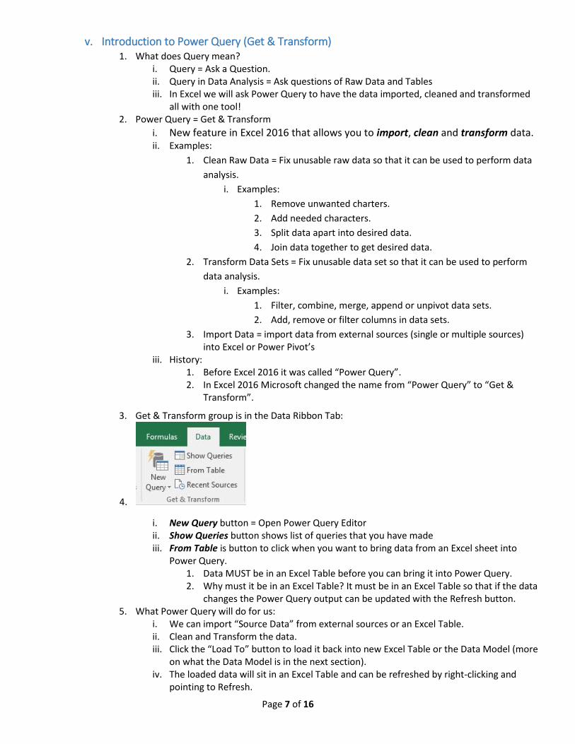
3. Get & Transform group is in the Data Ribbon Tab:

4.

i. New Query button = Open Power Query Editor ii. Show Queries button shows list of queries that you have made iii. From Table is button to click when you want to bring data from an Excel sheet into

Power Query. 1. Data MUST be in an Excel Table before you can bring it into Power Query. 2. Why must it be in an Excel Table? It must be in an Excel Table so that if the data

changes the Power Query output can be updated with the Refresh button. 5. What Power Query will do for us:

i. We can import “Source Data” from external sources or an Excel Table. ii. Clean and Transform the data. iii. Click the “Load To” button to load it back into new Excel Table or the Data Model (more

on what the Data Model is in the next section). iv. The loaded data will sit in an Excel Table and can be refreshed by right-clicking and

pointing to Refresh.

Page 8 of 16

6. This this video we will see three examples of how to use Power Query:

i. Goal: Convert Improper Data Set into Proper Data Set: 1) Clean Data, 2) Make PivotTable, 3) Have Cleaning Data and PivotTable UPDATE when Source Data Changes.

1. Convert Excel Data to Excel Table in order to get it into Power Query i. With single cell in Excel Table, click “From Table” button in the Get &

Transform group in the Data Ribbon Tab. 2. In Power Query Editor:

i. Break Product, Date and Region Fields apart into 3 Separate Fields 1. We will use the “Split Column” button in the Transform group in

the Power Query Home Ribbon Tab. 2. “Delimiter” means “Character that separates ‘Fields’ or ‘Bits of

Data’”. ii. Be sure to Name your Query.

iii. Be sure to check the Data Type for each Field. iv. Load Back to Excel

1. Click “Close & Load” in Close group in Power Query Home Ribbon Tab.

3. Make PivotTable. 4. Add new set of records:

i. You can paste whole new set of records below an Excel Table, and it will incorporate the new records into the data set.

5. Refresh Power Query output. 6. Refresh PivotTable.

ii. Goal: Unpivot a Crosstabulated Table into a proper data set so we can perform sort, filter and PivotTable on Proper Data Set.

1. When you “Unpivot” a Crosstabulated table: i. Row Headers becomes a single column

ii. Column headers become a single column iii. Numbers on inside of Crosstabulated table become a single column.

2. Convert Crosstabulated table to an Excel Table. 3. Click “From Table” button in the Get & Transform group in the Data Ribbon Tab. 4. In Power Query Editor:

i. Select the first column, Right-click, then click on “Unpivot Other Columns”

ii. Be sure to Name your Query. iii. Be sure to check the Data Type for each Field. iv. Load Back to Excel v. Click “Close & Load” in Close group in Power Query Home Ribbon Tab.

5. Why do we want to Unpivot a Crosstabulated Table into a Proper Data Set? i. Because once we have data in a Proper Data Set, we can use data

analysis features like Sort, Filter, PivotTable.

iii. Goal: 1) Import multiple files that contain more than one million rows of data and combine them into a single table.

1. See “Power Query and Power Pivot Data Model Example” on next page. 7. Later in the class we will learn more about Power Query (Get & Transform).

Page 9 of 16

vi. Introduction to Power Pivot and the Data Model 1. Power Pivot is like a super charged PivotTable that has its own database called the “Data

Model”. 2. Advantages of Power Pivot & Data Model over a normal PivotTable:

i. You can have tables that are millions of rows tall. 1. The Data Model is a Columnar Database that efficiently stores big data (file size

can be much smaller than original data), much more than a normal Excel sheet. ii. You can have more than one table in a PivotTable Field List and drag and drop fields

from both tables into a single PivotTable report. 1. The Data Model allows use to build Relationships between tables, just like we

did in Access. iii. You can build formulas for your PivotTable. (WE WILL DO THIS LATER IN THE CLASS).

1. The Data Model contains a new formula language called DAX (Data Analysis Expressions).

2. Compared to normal formulas in Excel that we put into cells, DAX Formulas can be dropped into a PivotTable and:

i. Will adapt to any conditions/criteria/filters that you drop into the Row, Column, Filter or Slicer area of a PivotTable.

ii. Calculate quickly because of how they interact with the Columnar Database.

3. We will look at some DAX Formula later in the class. In this section of the class, we are just getting an introduction to Power Pivot and the Data Model.

3. Power Query and Power Pivot Data Model Example:

i. Goal: 1. Import multiple text files that contain more than one million rows of data and

combine (transform) them into a single table. 2. Create a relationship between Newly Combined Table and a Lookup Table. 3. Create a PivotTable from two tables.

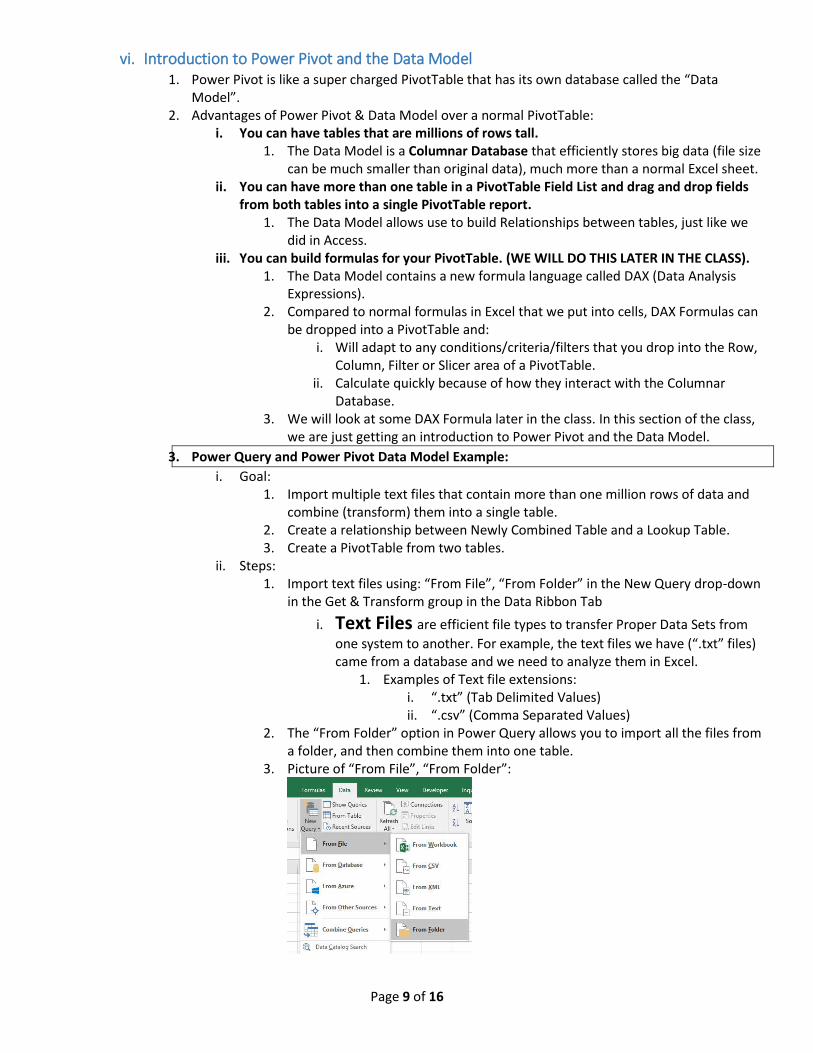
ii. Steps: 1. Import text files using: “From File”, “From Folder” in the New Query drop-down

in the Get & Transform group in the Data Ribbon Tab

i. Text Files are efficient file types to transfer Proper Data Sets from

one system to another. For example, the text files we have (“.txt” files) came from a database and we need to analyze them in Excel.

1. Examples of Text file extensions: i. “.txt” (Tab Delimited Values) ii. “.csv” (Comma Separated Values)

2. The “From Folder” option in Power Query allows you to import all the files from a folder, and then combine them into one table.

3. Picture of “From File”, “From Folder”:

Page 10 of 16

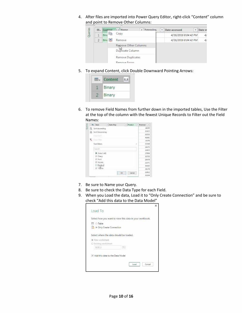
4. After files are imported into Power Query Editor, right-click “Content” column and point to Remove Other Columns:

5. To expand Content, click Double Downward Pointing Arrows:

6. To remove Field Names from further down in the imported tables, Use the Filter at the top of the column with the fewest Unique Records to Filter out the Field Names:

7. Be sure to Name your Query. 8. Be sure to check the Data Type for each Field. 9. When you Load the data, Load it to “Only Create Connection” and be sure to

check “Add this data to the Data Model”

Page 11 of 16

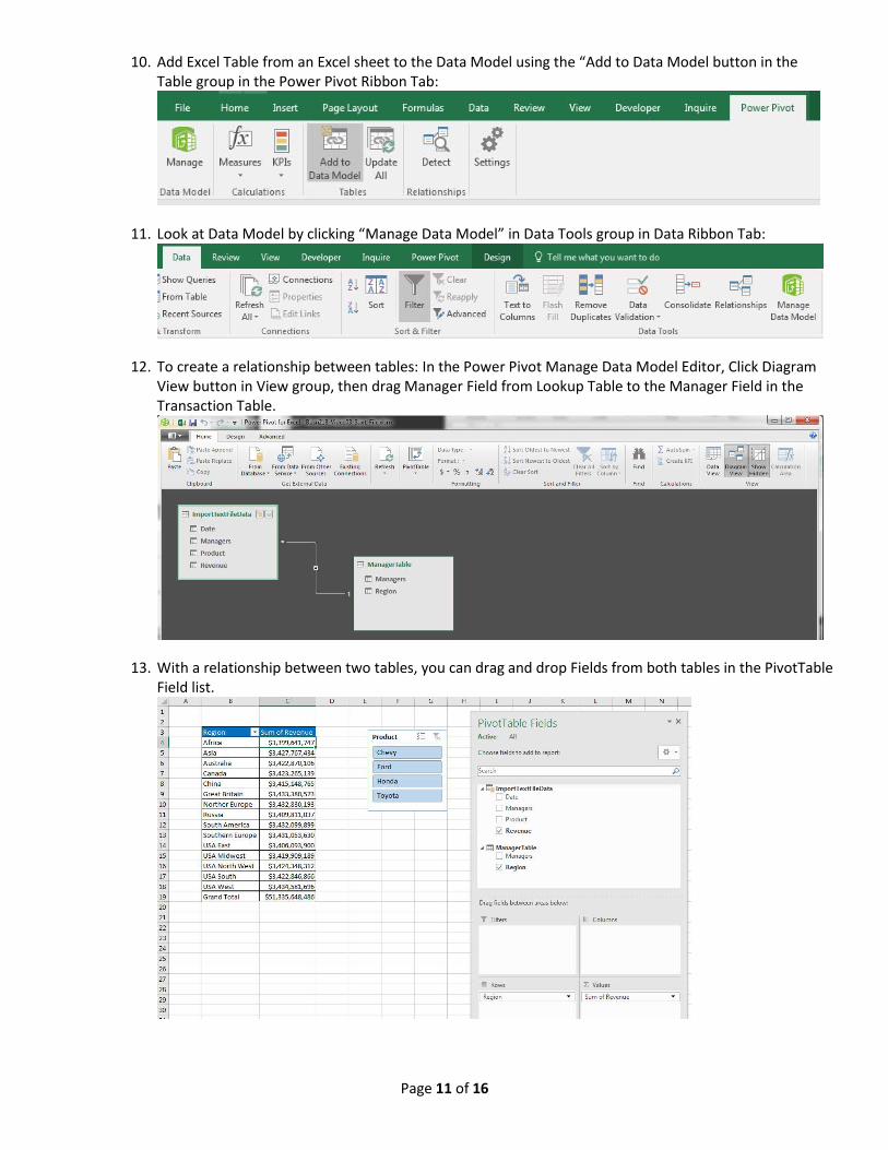
10. Add Excel Table from an Excel sheet to the Data Model using the “Add to Data Model button in the Table group in the Power Pivot Ribbon Tab:

11. Look at Data Model by clicking “Manage Data Model” in Data Tools group in Data Ribbon Tab:

12. To create a relationship between tables: In the Power Pivot Manage Data Model Editor, Click Diagram View button in View group, then drag Manager Field from Lookup Table to the Manager Field in the Transaction Table.

13. With a relationship between two tables, you can drag and drop Fields from both tables in the PivotTable Field list.

Page 12 of 16

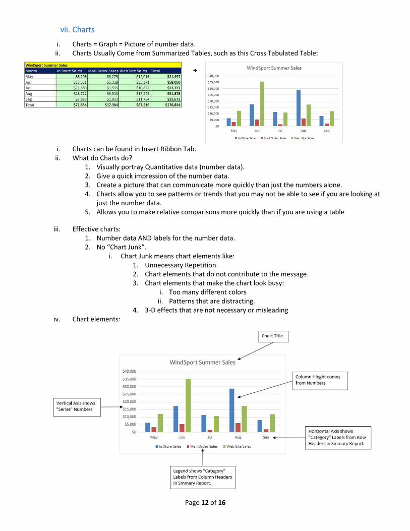
vii. Charts

i. Charts = Graph = Picture of number data. ii. Charts Usually Come from Summarized Tables, such as this Cross Tabulated Table:

i. Charts can be found in Insert Ribbon Tab.

ii. What do Charts do? 1. Visually portray Quantitative data (number data). 2. Give a quick impression of the number data. 3. Create a picture that can communicate more quickly than just the numbers alone. 4. Charts allow you to see patterns or trends that you may not be able to see if you are looking at

just the number data. 5. Allows you to make relative comparisons more quickly than if you are using a table

iii. Effective charts: 1. Number data AND labels for the number data. 2. No “Chart Junk”.

i. Chart Junk means chart elements like: 1. Unnecessary Repetition. 2. Chart elements that do not contribute to the message. 3. Chart elements that make the chart look busy:

i. Too many different colors ii. Patterns that are distracting.

4. 3-D effects that are not necessary or misleading iv. Chart elements:

Page 13 of 16

v. Types of Charts: 1. Column Charts:

i. Show relative differences (in numbers) across categories (labels). ii. Height of columns convey number.

iii. Categories are listed on Horizontal Axis or in Legend.

2. Bar Charts: i. Same as column, except: Columns are shown horizontal and are called bars. ii. Bars can emphasize the differences between the categories better than a column chart. iii. Sometimes Bars show long labels better than Column.

3. Stacked Column Charts:

i. Good for displaying crosstabulation.

ii. Emphasis is on comparing the categories listed in the horizontal axis

iii. Excel:

1. If the number of row headers are equal or greater than to the number of

column headers, row headers show up on horizontal axis and column headers in

legend. If not, they are reversed. (You can switch this with the Switch button in

the Chart Tools Design Ribbon Tab)

4. Clustered Column Charts:

i. Good for displaying crosstabulation.

ii. Emphasis is on comparing the categories listed in the legend

iii. Excel:

1. If the number of row headers are equal or greater than to the number of

column headers, row headers show up on horizontal axis and column headers in

legend. If not, they are reversed. (You can switch this with the Switch button in

the Chart Tools Design Ribbon Tab)

5. Pie Charts: i. Parts that make up the whole. ii. Don’t included totals in a Pie Chart.

6. It is more effective to use Column or Bar Charts than Pie Charts:

i. Research shows that Column or Bar Charts convey relative differences more effectively than Pie Charts.

ii. In recent years data analysis practitioners tend to use Column or Bar Charts rather than Pie Charts.

7. Line Charts: i. One number on vertical axis, category on horizontal axis ii. Great for show trends over time.

8. X-Y Scatter i. Chart that shows the relationship between two number variables (like study time for a

test and score on test).

ii. One number on vertical axis, one number on horizontal axis:

1. Horizontal Axis = Independent Variable = x.

2. Vertical Axis = Dependent Variable = f(x) = y

iii. Always put X values in Left Most Column in the Table of Data (in order for chart engine

to interpret the data correctly).

iv. Add Regression Line and Equation and R Square:

1. Right-click plotted scatter markers

2. Add Trendline

3. Select Linear

4. Check check box for Show Equation

Page 14 of 16

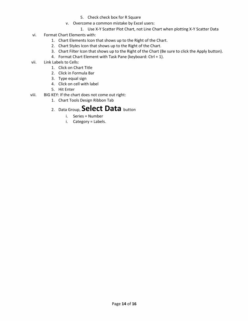
5. Check check box for R Square

v. Overcome a common mistake by Excel users:

1. Use X-Y Scatter Plot Chart, not Line Chart when plotting X-Y Scatter Data

vi. Format Chart Elements with: 1. Chart Elements Icon that shows up to the Right of the Chart. 2. Chart Styles Icon that shows up to the Right of the Chart. 3. Chart Filter Icon that shows up to the Right of the Chart (Be sure to click the Apply button). 4. Format Chart Element with Task Pane (keyboard: Ctrl + 1).

vii. Link Labels to Cells: 1. Click on Chart Title 2. Click in Formula Bar 3. Type equal sign 4. Click on cell with label 5. Hit Enter

viii. BIG KEY: If the chart does not come out right: 1. Chart Tools Design Ribbon Tab

2. Data Group, Select Data button

i. Series = Number i. Category = Labels.

Page 15 of 16

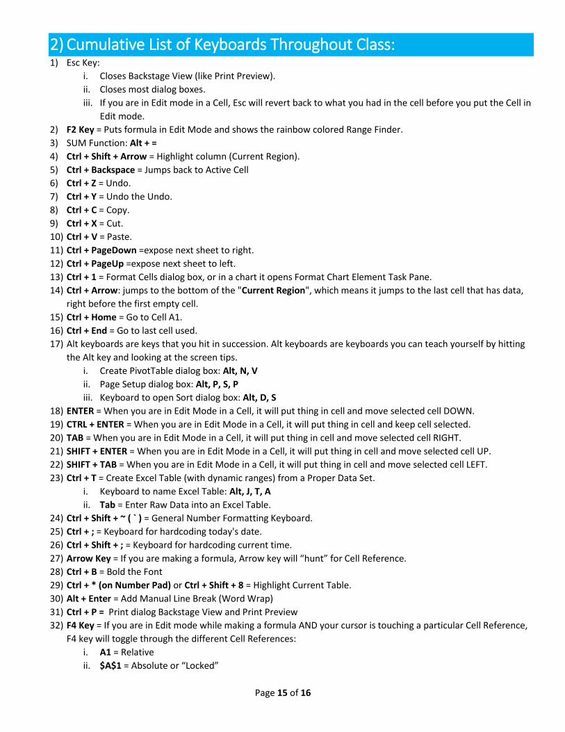
2) Cumulative List of Keyboards Throughout Class: 1) Esc Key:

i. Closes Backstage View (like Print Preview).

ii. Closes most dialog boxes.

iii. If you are in Edit mode in a Cell, Esc will revert back to what you had in the cell before you put the Cell in

Edit mode.

2) F2 Key = Puts formula in Edit Mode and shows the rainbow colored Range Finder.

3) SUM Function: Alt + =

4) Ctrl + Shift + Arrow = Highlight column (Current Region).

5) Ctrl + Backspace = Jumps back to Active Cell

6) Ctrl + Z = Undo.

7) Ctrl + Y = Undo the Undo.

8) Ctrl + C = Copy.

9) Ctrl + X = Cut.

10) Ctrl + V = Paste.

11) Ctrl + PageDown =expose next sheet to right.

12) Ctrl + PageUp =expose next sheet to left.

13) Ctrl + 1 = Format Cells dialog box, or in a chart it opens Format Chart Element Task Pane.

14) Ctrl + Arrow: jumps to the bottom of the "Current Region", which means it jumps to the last cell that has data,

right before the first empty cell.

15) Ctrl + Home = Go to Cell A1.

16) Ctrl + End = Go to last cell used.

17) Alt keyboards are keys that you hit in succession. Alt keyboards are keyboards you can teach yourself by hitting

the Alt key and looking at the screen tips.

i. Create PivotTable dialog box: Alt, N, V

ii. Page Setup dialog box: Alt, P, S, P

iii. Keyboard to open Sort dialog box: Alt, D, S

18) ENTER = When you are in Edit Mode in a Cell, it will put thing in cell and move selected cell DOWN.

19) CTRL + ENTER = When you are in Edit Mode in a Cell, it will put thing in cell and keep cell selected.

20) TAB = When you are in Edit Mode in a Cell, it will put thing in cell and move selected cell RIGHT.

21) SHIFT + ENTER = When you are in Edit Mode in a Cell, it will put thing in cell and move selected cell UP.

22) SHIFT + TAB = When you are in Edit Mode in a Cell, it will put thing in cell and move selected cell LEFT.

23) Ctrl + T = Create Excel Table (with dynamic ranges) from a Proper Data Set.

i. Keyboard to name Excel Table: Alt, J, T, A

ii. Tab = Enter Raw Data into an Excel Table.

24) Ctrl + Shift + ~ ( ` ) = General Number Formatting Keyboard.

25) Ctrl + ; = Keyboard for hardcoding today's date.

26) Ctrl + Shift + ; = Keyboard for hardcoding current time.

27) Arrow Key = If you are making a formula, Arrow key will “hunt” for Cell Reference.

28) Ctrl + B = Bold the Font

29) Ctrl + * (on Number Pad) or Ctrl + Shift + 8 = Highlight Current Table.

30) Alt + Enter = Add Manual Line Break (Word Wrap)

31) Ctrl + P = Print dialog Backstage View and Print Preview

32) F4 Key = If you are in Edit mode while making a formula AND your cursor is touching a particular Cell Reference,

F4 key will toggle through the different Cell References:

i. A1 = Relative

ii. $A$1 = Absolute or “Locked”

Page 16 of 16

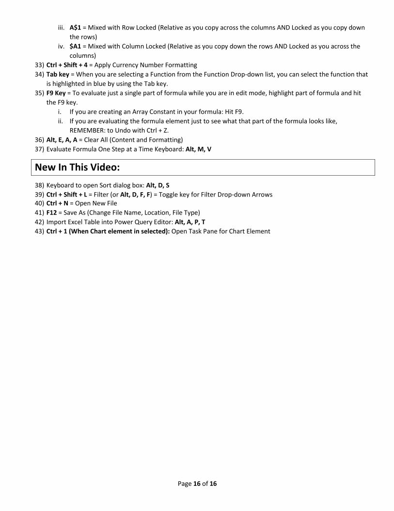
iii. A$1 = Mixed with Row Locked (Relative as you copy across the columns AND Locked as you copy down

the rows)

iv. $A1 = Mixed with Column Locked (Relative as you copy down the rows AND Locked as you across the

columns)

33) Ctrl + Shift + 4 = Apply Currency Number Formatting

34) Tab key = When you are selecting a Function from the Function Drop-down list, you can select the function that

is highlighted in blue by using the Tab key.

35) F9 Key = To evaluate just a single part of formula while you are in edit mode, highlight part of formula and hit

the F9 key.

i. If you are creating an Array Constant in your formula: Hit F9.

ii. If you are evaluating the formula element just to see what that part of the formula looks like,

REMEMBER: to Undo with Ctrl + Z.

36) Alt, E, A, A = Clear All (Content and Formatting)

37) Evaluate Formula One Step at a Time Keyboard: Alt, M, V

New In This Video:

38) Keyboard to open Sort dialog box: Alt, D, S

39) Ctrl + Shift + L = Filter (or Alt, D, F, F) = Toggle key for Filter Drop-down Arrows 40) Ctrl + N = Open New File

41) F12 = Save As (Change File Name, Location, File Type)

42) Import Excel Table into Power Query Editor: Alt, A, P, T

43) Ctrl + 1 (When Chart element in selected): Open Task Pane for Chart Element