Embed Size (px)
Citation preview

Topics in importance sampling and derivatives pricing
JOHAN NYKVIST
Doctoral ThesisStockholm, Sweden 2015

TRITA-MAT-A 2015:02ISRN KTH/MAT/A-15/02-SEISBN 978-91-7595-445-5
Department of MathematicsRoyal Institute of Technology
100 44 Stockholm, Sweden
Akademisk avhandling som med tillstånd av Kungl Tekniska Högskolan framlägges till of-fentlig granskning för avläggande av teknologie doktorsexamen, tisdagen den 3 mars 2015klockan 14.00 i sal F3, Lindstedtsvägen 26, Kungl Tekniska Högskolan, Stockholm.
© Johan Nykvist, 2015
Print: Universitetsservice US AB, Stockholm, 2015

Abstract
This thesis consists of four papers, presented in Chapters 2-5, on the topics of derivativespricing and importance sampling for stochastic processes.
In the first paper a model for the evolution of the forward density of the future valueof an asset is proposed. The model is constructed with the aim of being both simple andrealistic, and avoid the need for frequent re-calibration. The model is calibrated to liquidoptions on the S&P 500 index and an empirical study illustrates that the model provides agood fit to option price data.
In the last three papers of this thesis efficient importance sampling algorithms are de-signed for computing rare-event probabilities in the setting of stochastic processes. Thealgorithms are based on subsolutions of partial differential equations of Hamilton-Jacobitype and the construction of appropriate subsolutions is facilitated by a minmax represen-tation involving the Mañé potential.
In the second paper, a general framework is provided for the case of one-dimensionaldiffusions driven by Brownian motion. An analytical formula for the Mañé potential isprovided and the performance of the algorithm is analyzed in detail for geometric Brownianmotion and for the Cox-Ingersoll-Ross process. Depending on the choice of the parametersof the models, the importance sampling algorithm is either proven to be asymptoticallyoptimal or its good performance is demonstrated in numerical investigations.
The third paper extends the results from the previous paper to the setting of high-dimensional stochastic processes. Using the method of characteristics, the partial differen-tial equation for the Mañé potential is rewritten as a system of ordinary differential equa-tions which can be efficiently solved. The methodology is used to estimate loss probabil-ities of large portfolios in the Black-Scholes model and in the stochastic volatility modelproposed by Heston. Numerical experiments indicate that the algorithm yields significantvariance reduction when compared with standard Monte-Carlo simulation.
In the final paper, an importance sampling algorithm is proposed for computing theprobability of voltage collapse in a power system. The power load is modeled by a high-dimensional stochastic process and the sought probability is formulated as an exit problemfor the diffusion. A particular challenge is that the boundary of the domain cannot becharacterized explicitly. Simulations for two power systems shows that the algorithm canbe effectively implemented and provides a viable alternative to existing system risk indices.
The thesis begins with a historical review of mathematical finance, followed by anintroduction to importance sampling for stochastic processes.
iii

Sammanfattning
Avhandlingen består av fyra vetenskapliga artiklar, presenterade i kapitel 2-5, ochbehandlar prissättning av finansiella derivat samt viktad simulering (importance sam-pling) för stokastiska processer.
I den första artikeln föreslås en modell för täthetsfunktionen och dess dynamik övertid för ett framtida värde av en tillgång, med avseende på det så kallade "forwardmåt-tet". Syftet med modellen är att den ska vara enkel och realistisk samt undvika behovetav frekvent omkalibrering. Modellen kalibreras till priser på likvida optioner på S&Pindexet och en empirisk studie visar att modellen ger en bra passning till prisdata påEuropeiska optioner.
I de tre avslutande artiklarna i avhandlingen utformas algoritmer för viktad simu-lering som syftar till att beräkna sannolikheter för extrema händelser för stokastiskaprocesser. Algoritmerna baseras på sublösningar till partiella differentialekvationeroch konstruktionen av lämpliga sublösningar genomförs med hjälp av en minmax-representation som involverar Mañé-potentialen.
I den andra artikeln framställs ett generellt ramverk för en-dimensionella stokastiskaprocesser som drivs av Brownsk rörelse. Ett analytiskt uttryck tas fram för Mañé-potentialen och prestandan för algoritmen analyseras i detalj för geometrisk Brownskrörelse samt för Cox-Ingersoll-Ross-processen. För speciella val av modellparame-trarna bevisar vi att importance algoritmen är asymptotiskt optimal.
I den tredje artikeln utvidgas resultaten från den föregående artikeln till fler-dimen-sionella stokastiska processer. Med hjälp av "method of characteristics" kan den par-tiella differentialekvationen för Mañé-potentialen skrivas om som ett system av or-dinära differentialekvationer vilket kan lösas explicit. Metoden används för att beräknasannolikheter för stora förluster i finansiella portföljer då de underliggande prisernabeskrivs av Black-Scholes-modellen samt av den stokastiska volatilitetsmodellen fram-tagen av Heston. Numeriska experiment visar att algoritmen ger en signifikant varian-sreduktion jämfört med vanlig Monte-Carlo simulering.
I den avslutande artikeln föreslås en algoritm för viktad simulering för att beräknasannolikheten för spänningskollaps i ett elsystem. Lasterna i systemet modelleras somen hög-dimensionell diffusionsprocess och den sökta sannolikheten beräknas som ett"exit problem" för diffusioner. Det centrala problemet för elsystem är att det stabilaområdet inte kan karaktäriseras explicit. Simuleringar för två elsystem visar att algorit-men kan implementeras på ett effektivt sätt och att den kan användas som ett alternativtill existerande beräkningsmetoder för att bedöma risker i storskaliga system..
Avhandlingen börjar med en historisk överblick av finansmatematik samt en intro-duktion till viktad simulering för stokastiska processer.
iv

Acknowledgments
My time as a graduate student is coming to an end and it is time to thank all who havemade this thesis possible.
My deepest gratitude goes to Associate Professor Filip Lindskog who has been myadvisor for the past five years. I am truly grateful that I was given the opportunity to workwith him. His qualities, as a researcher and as a teacher, have had a great impact on me.
My warmest thanks to Associate Professor Henrik Hult who has been my co-authorduring my time at KTH. He introduced me to the field of importance sampling and providedme with a new direction when I struggled with my research.
Many thanks to my colleagues at the division of Mathematical Statistics for welcomingme to the department and for providing an inspiring working environment.
I would like to thank my present and former officemates. Thanks Dr Thorbjörn Gud-mundsson and Björn Löfdahl for fruitful discussions and for my progression as a tabletennis player. Special thanks to Dr Pierre Nyquist for his contributions to this thesis andfor the dreadful running sessions on Djurgården.
Thanks to the crew in Puppy Triathlete Society and in particular to Henke and Perra.Had it not been for you, it is likely that this thesis would have been finished a long timeago. On the other hand, I would not have the great memories that I have today.
I am forever grateful to my parents and family. You have always been there for me andwithout your support I would not be the person I am today.
Finally, I want to thank the person who is most important to me. Thank you Emelie forkeeping up with the late nights, the bad morning mood and all my other flaws. You meanthe world to me.
Stockholm, January 2015
Johan Nykvist
v


Contents
Abstract iii
Acknowledgments v
Contents vii
1 Introduction 11.1 Time consistency in option pricing models . . . . . . . . . . . . . . . . . 1
1.1.1 The Black-Scholes equation . . . . . . . . . . . . . . . . . . . . 31.1.2 Stochastic volatility models . . . . . . . . . . . . . . . . . . . . 61.1.3 Local volatility models . . . . . . . . . . . . . . . . . . . . . . . 71.1.4 Time consistency in option pricing models . . . . . . . . . . . . 8
1.2 Importance sampling . . . . . . . . . . . . . . . . . . . . . . . . . . . . 101.2.1 Importance sampling and Hamilton-Jacobi equations . . . . . . . 121.2.2 Construction of subsolutions based on the Mañé potential . . . . 151.2.3 The method of characteristics . . . . . . . . . . . . . . . . . . . 171.2.4 Efficient importance sampling for scaled Brownian motion . . . . 19
1.3 Summary of papers . . . . . . . . . . . . . . . . . . . . . . . . . . . . . 231.4 References . . . . . . . . . . . . . . . . . . . . . . . . . . . . . . . . . . 26
2 A simple time-consistent model for the forward density process 292.1 Introduction . . . . . . . . . . . . . . . . . . . . . . . . . . . . . . . . . 312.2 The spot price at maturity . . . . . . . . . . . . . . . . . . . . . . . . . . 352.3 The forward price processes . . . . . . . . . . . . . . . . . . . . . . . . 37
2.3.1 Tracking the Brownian particle in continuous time . . . . . . . . 382.3.2 The forward price dynamics . . . . . . . . . . . . . . . . . . . . 412.3.3 Explicit computations in the case n = 2 . . . . . . . . . . . . . . 43
2.4 Calibration and evaluation of the model . . . . . . . . . . . . . . . . . . 452.4.1 The initial calibration and model specification . . . . . . . . . . . 462.4.2 Tracking the Brownian particle in discrete time . . . . . . . . . . 49
2.5 Proof of Proposition 2.2.1 . . . . . . . . . . . . . . . . . . . . . . . . . . 552.6 References . . . . . . . . . . . . . . . . . . . . . . . . . . . . . . . . . . 59
vii

3 A note on efficient importance sampling for one-dimensional diffusions 613.1 Introduction . . . . . . . . . . . . . . . . . . . . . . . . . . . . . . . . . 633.2 Importance sampling and Hamilton-Jacobi equations . . . . . . . . . . . 65
3.2.1 The subsolution approach to efficient importance sampling . . . . 653.2.2 Construction of subsolutions based on the Mañé potential . . . . 68
3.3 The Mañé potential and the performance of algorithms . . . . . . . . . . 693.3.1 Computing the Mañé potential . . . . . . . . . . . . . . . . . . . 70
3.4 Geometric Brownian motion . . . . . . . . . . . . . . . . . . . . . . . . 713.5 The Cox-Ingersoll-Ross process . . . . . . . . . . . . . . . . . . . . . . 763.6 References . . . . . . . . . . . . . . . . . . . . . . . . . . . . . . . . . . 80
4 Efficient importance sampling to compute loss probabilities in financial port-folios 834.1 Introduction . . . . . . . . . . . . . . . . . . . . . . . . . . . . . . . . . 854.2 The Delta-Gamma approximation . . . . . . . . . . . . . . . . . . . . . 884.3 Importance sampling and Hamilton-Jacobi equations . . . . . . . . . . . 90
4.3.1 The subsolution approach to efficient importance sampling . . . . 904.3.2 Construction of subsolutions based on the Mañé potential . . . . 93
4.4 The Black-Scholes model . . . . . . . . . . . . . . . . . . . . . . . . . . 944.4.1 Computing the Mañé potential . . . . . . . . . . . . . . . . . . . 954.4.2 On efficiency of the importance sampling algorithm . . . . . . . . 994.4.3 Numerical experiments . . . . . . . . . . . . . . . . . . . . . . . 101
4.5 The Heston model . . . . . . . . . . . . . . . . . . . . . . . . . . . . . . 1084.5.1 Computing the Mañé potential . . . . . . . . . . . . . . . . . . . 1094.5.2 Numerical experiments . . . . . . . . . . . . . . . . . . . . . . . 115
4.6 Proof of Theorem 4.4.3 . . . . . . . . . . . . . . . . . . . . . . . . . . . 1174.7 References . . . . . . . . . . . . . . . . . . . . . . . . . . . . . . . . . . 121
5 Efficient importance sampling to assess the risk of voltage collapse in powersystems 1235.1 Introduction . . . . . . . . . . . . . . . . . . . . . . . . . . . . . . . . . 1255.2 Power systems and voltage stability . . . . . . . . . . . . . . . . . . . . 1295.3 Importance sampling and Hamilton-Jacobi equations . . . . . . . . . . . 132
5.3.1 The subsolution approach to efficient importance sampling . . . . 1325.3.2 Construction of subsolutions based on the Mañé potential . . . . 135
5.4 Design of importance algorithms for Ornstein-Uhlenbeck processes . . . 1365.4.1 Escape from a symmetric domain . . . . . . . . . . . . . . . . . 1395.4.2 Escape from an asymmetric domain . . . . . . . . . . . . . . . . 1415.4.3 Voltage collapse in a 9-bus power system . . . . . . . . . . . . . 1425.4.4 Voltage collapse in a 39-bus power system . . . . . . . . . . . . . 144
5.5 Summary . . . . . . . . . . . . . . . . . . . . . . . . . . . . . . . . . . 1455.6 References . . . . . . . . . . . . . . . . . . . . . . . . . . . . . . . . . . 146
viii

Introduction
1.1 Time consistency in option pricing models
In the field of mathematical finance a fundamental problem for researchers and practi-tioners is the valuation of financial derivatives. Briefly, a financial derivative is a contractbetween a seller and a buyer whose cash flow is expressed in terms of the future value(s)of an asset.
Financial derivatives make future risk tradable and has at least two main uses. Firstly,by taking positions in financial derivatives, companies and financial institutions can reduceor eliminate uncertainty about the future state of the market. This is called hedging. Sec-ondly, financial derivatives can be used for pure investment. Derivatives can be used tospeculate in the future value of an asset price without buying the asset itself.
The canonical example of a financial derivative is the European call option. A Europeancall option written on ST , where ST denotes the value of an asset at the future time T > 0,with strike price K, gives the holder of the contract the right, but not the obligation, tobuy the asset at time T for the predetermined price K. Since the right is only exercised ifST > K, it follows that the value of the option at time T is max(ST−K, 0) = (ST−K)+.The price of the derivative at the time T of maturity is therefore known. But what is theprice of the option at time t < T ?
Before we discuss the valuation of options and other financial derivatives in a generalsetting, let us consider a simple market model consisting of a stock and a bond maturingtomorrow. The bond is risk-free which means that given its value today we know its valuetomorrow. For simplicity, let us assume that the risk-free interest rate is zero so that theprice of the bond equals one today and tomorrow:
B0 = B1 = 1.
The stock on the other hand is a risky asset, meaning that its value today is known butthe value tomorrow is unknown. Suppose that S0 = 1 and that S1 is a random variabledepending on the unknown state ω ∈ Ω. To keep things simple, suppose that Ω = u, dconsists of only two elements, where u stands for "up", d stands for "down". Define S1(ω)by
S1(ω) =
2, ω = u,
1/2, ω = d.
1

2 CHAPTER 1. INTRODUCTION
Assume that a third asset is introduced on the market in the form of a European calloption written on S1 with strike price 1. Then C1 is a random variable defined by
C1(ω) =
1, ω = u,
0, ω = d.
The task is to assign the option a fair price which is consistent with the prices of the existingassets on the market. The terminology fair price is a bit vague, but will soon be made moreprecise.
To determine the fair price, suppose that at t = 0 we buy a portfolio consisting of 2/3shares of the stock and −1/3 bonds. Then the value Π1 of the portfolio tomorrow is givenby
Π1(ω) =
23 · 2− 1
3 · 1 = 1, ω = u,23 · 1
2 − 13 · 1 = 0, ω = d.
The portfolio replicates the cash flow of the call option in the sense that Π1 = C1, and iscalled the replicating portfolio of the call option.
The price of the portfolio today is given by
Π0 =2
3S0 −
1
3B0 =
1
3.
We argue that since C1 = Π1, it must also hold that C0 = Π0. To see that this is the fairprice of the option, suppose that C0 = 1/2. Then, we buy the replicating portfolio todayand simultaneously sell the call option, thereby making an initial profit of C0−Π0 = 1/6.Tomorrow, the two cash flows cancel out independently of whether ω equals u or d, soregardless of how the stock evolves we make a profit of 1/6. On the other hand, if C0 <1/3 we can make a risk-free profit by buying the option and short selling the portfolio. Ineither case, if C0 is anything else than 1/3 there is an arbitrage-opportunity in the market:a possibility to make a profit without any risk and without an initial investment. The fairprice of the option is therefore the price which renders no arbitrage opportunities to themarket participants, in this case C0 = 1/3.
Suppose that the future market states is governed by the probability measure P. Noticethat if P(u) = P(d) = 1/2, then the expected rate of return of the stock is 1.25 whereasthe rate of return of the risk-free bond is 1. Thus, the additional risk imposed by takingpositions in the stock is compensated for by a higher expected rate of return. However, theprobabilities P(u) and P(d) did not show up in the arbitrage-free value of the option.
For the moment, let us assume that the market dynamics are driven by another proba-bility measure Q which is equivalent to P, written Q ∼ P, in the sense that Q(ω) = 0 ifand only if P(ω) = 0. In particular, we assume that under Q the expected rate of returnof the stock equals the rate of return of the bond. It is easily seen that Q(u) = 1/3 andQ(d) = 2/3 is the unique solution to EQ[S1] = 1. For a risk-neutral market participant,taking positions in the stock is equally attractive to taking positions in the bond. There-fore, the measure Q is commonly referred to as the risk-neutral measure. Since S (or ratherS/B) is a martingale under Q it is also often called a martingale measure for S.

1.1. TIME CONSISTENCY IN OPTION PRICING MODELS 3
Now, computing the expected value of C1 under the risk-neutral measure yields
EQ[C1] =1
3· 1 +
2
3· 0 =
1
3.
Thus, the arbitrage-free price of the option is given by the (discounted) expected value ofthe payoff, where the expectation is taken with respect to the risk-neutral measure. This isnot a coincidence, but rather the very foundation of arbitrage pricing.
Consider a market model consisting of asset prices S0, S1, . . . , Sn on a filtered proba-bility space (Ω, Ft0≤t≤T ,P). Let S0 denote the numeraire process and assume that S0
is a strictly positive process. Typically, S0 will denote the bank account or the price of azero-coupon bond. The market consisting of the n + 1 assets is free of arbitrage if thereexists an equivalent martingale measure, i.e. a probability measure Q with Q ∼ P andsuch that the processes
S1
S0, . . . ,
SnS0
are Q-martingales. This is called the first fundamental theorem of asset pricing. Thesecond fundamental theorem states that if the equivalent martingale measure is unique,then the market is complete in the sense that any new derivative contract can be replicatedby existing contracts.
Let X be a contingent claim, i.e. an FT -measurable random variable, and let Π(t, St)denote the value of X at time t < T . If the market is free of arbitrage, the arbitrage-freeprice Π(t, St) is given by the risk-neutral valuation formula
Π(t, St) = S0(t) EQ[ X
S0(T )|Ft]. (1.1)
In the literature, the pricing of derivatives as conditional expectations is commonly re-ferred to as the martingale approach. The theory was developed in [24], [31], and [25] andhas since then been extended and considerably generalised in [12], [36], and [13]. Thelatter articles involve deep mathematics and are rather technical, so for a more accessiblepresentation, the interested reader is referred to [3].
The martingale approach to pricing derivatives is one of the two main pricing ap-proaches used by researchers and practitioners. In the other approach, the arbitrage-freeprice of a contingent claim is given by the solution to a partial differential equation. Thisapproach was developed in the seminal paper [4] by Fischer Black and Myron Scholes andsimultaneously in [34] by Robert Merton. In the following section, we review the work in[4] which yields the famous Black-Scholes equation.
1.1.1 The Black-Scholes equation
In the beginning of the 20th century, Louis Bachelier defended his thesis "Théorie dela spéculation" [2] and at the same time gave birth to the modern mathematical finance.

4 CHAPTER 1. INTRODUCTION
Bachelier derived the mathematics of Brownian motion and used the one-dimensional ver-sion to model stock price dynamics and compute option prices. In the 1940’s, Kiyoshi Itôused the Brownian motion to define stochastic differential equations of the form
dXt = µ(Xt)dt+ σ(Xt)dWt, X0 = x0,
where W is a standard Brownian motion. Some years later in [28] he derived what is nowknown as Itô’s lemma: for any twice differentiable function f , it holds that
df(Xt) = f ′(Xt)dXt +1
2f ′′(Xt)d〈X〉t, (1.2)
where 〈·〉 denotes the quadratic variation. Using the formula (1.2), researchers and prac-titioners were able to derive new stochastic differential equations from existing ones. Inparticular, researchers could use stochastic processes to model stock price dynamics.
The Black-Scholes market consists of a stock and a bond and the market dynamicsunder the probability measure P are given by
dSt = µStdt+ σStdWt,
dBt = rBtdt,
where µ, σ are constants, W is a standard Brownian motion, and r is the continuouslycompounded risk-free interest rate.
Following the work of [4], let V (t, St) denote the value at time t < T of a Europeancall option written on ST with strike price K. The value V (T, ST ) = (ST −K)+ of theoption at maturity is known. To compute the value at t < T , consider a portfolio consistingof a short position of size one in the option and a position of size ∂V/∂S in the underlyingasset. Let Π denote the value of the portfolio so that Π = −V + ∂V
∂S S. Over a time interval[t, t+ ∆t], the change in the portfolio value ∆Π is therefore given by
∆Π = −∆V +∂V
∂S∆S. (1.3)
Applying Itô’s formula to the function V (t, St) yields
dVt =(∂V∂t
+ µS∂V
∂S+
1
2σ2S2 ∂
2V
∂S2
)dt+ σS
∂V
∂SdWt.
Inserting the differentials ∆S and ∆V in (1.3) we obtain
∆Π =(− ∂V
∂S− 1
2σ2S2 ∂
2V
∂S2
)∆t.
Since the ∆W -term has vanished, the portfolio is risk-free. If the market is free of ar-bitrage, the rate of return of the risk-free portfolio must equal the rate of return of therisk-free bond. Thus,
∆Π = rΠ∆t,

1.1. TIME CONSISTENCY IN OPTION PRICING MODELS 5
or, equivalently,(− ∂V
∂S− 1
2σ2S2 ∂
2V
∂S2
)∆t = r
(− V +
∂V
∂S
)∆t.
Dividing both sides by ∆t yields the famous Black-Scholes equation
∂V
∂t(t, x) +
1
2σ2x2 ∂
2V
∂x2(t, x) + r
∂V
∂x(t, x)− rV (t, x) = 0,
V (T, x) = (x−K)+.
(1.4)
We find that the arbitrage-free price of a European call option can be computed asthe solution to the partial differential equation (1.4). In fact, the formula holds for anyderivative assuming that its value function V (t, x) is twice differentiable in x and oncein t. Pricing derivatives by solving partial differential equations is the other main pricingapproach used today and is often referred to as the partial differential equation approach.
In [4] the equation (1.4) is solved explicitly for the European call option and the re-sulting pricing formula is the famous Black-Scholes formula. The arbitrage-free price of aEuropean call option in the Black-Scholes model is given by
V (t, St) = N(d1)St −Ke−r(T−t)N(d2), (1.5)
where N(·) denotes the cumulative distribution function of a standard normal random vari-able, and
d1 =logSt − logK + (r − 1
2σ2)(T − t)
σ√T − t , d2 = d1 − σ
√T − t.
It is desirable that an option pricing model admits explicit formulas for European putand call options. The reason is that European options are often traded in large volumesso their prices can be considered given by the market and used as a basis for pricing morecomplex derivative contracts. In the classical approach to option pricing, the starting pointis a model for the evolution of the asset prices St0≤t≤T under the probability measureP. The corresponding dynamics under an equivalent martingale measure are then derivedand the price of a contingent claim is computed by the risk-neutral valuation formula (1.1).If the price of a European option can be evaluated efficiently, the model parameters canbe calibrated to quoted market prices for liquidly traded options. Given the accurate esti-mates of the model parameters, the model prices of other more complex derivatives can becomputed, analytically, numerically or by simulation.
In the Black-Scholes model, the only free parameter is the volatility σ. Given themarket price Ct of a European call option written on ST with strike price K, the impliedBlack-Scholes volatility, σBS , is the unique value of σ in (1.5) such that V (t, St) = Ct.We call it the implied volatility because it is implied from the market price. If the Black-Scholes model was correct, European options with different strikes and maturities writtenon a given stock would have the same implied volatilities. However, option price datatypically do not support the assumption of constant volatility. In the following sectionwe discuss an alternative class of models where the volatility is modeled by a stochasticprocess.

6 CHAPTER 1. INTRODUCTION
1.1.2 Stochastic volatility models
Empirical investigations show that log return sample standard deviations vary over time ina way that is not consistent with a constant volatility. In stochastic volatility models, theassumption of deterministic volatilities is relaxed and replaced by the assumption that thevolatility varies according to a stochastic differential equation. Over the last thirty years,various stochastic volatility models have been proposed including the models by Hull andWhite [27], Melino and Turnbull [33], Stein and Stein [39], Heston [26], and Scott [37].
For the calibration of a stochastic volatility model to market prices of European optionsit is desirable that the model admits explicit option pricing formulas which can be evaluatedefficiently. Among the models mentioned above, those of Stein and Stein and Heston yieldsemi-closed-form formulas for the price of a European option. They are semi-closed-formbecause both formulas involve an integral which must be computed numerically.
In the Stein-Stein model [39] it is assumed that the stock price follows a stochasticdifferential equation of the form
dSt = µStdt+ vtStdW1t , (1.6)
whereas the volatility vt evolves according to an Ornstein-Uhlenbeck process given by
dvt = κ(θ − vt)dt+ σdW 2t .
The main objection to the model is that the stock price and volatility processes are assumedto be uncorrelated and that the volatility process allows for negative volatilities. For eq-uities, market price dynamics typically show that changes in the equity price and changesin Black-Scholes implied volatilities are negatively correlated, see [23]. Nevertheless, be-cause prices of European options can be computed rather efficiently, the model has gainedsome popularity among practitioners.
In [26] an alternative model, known as the Heston model, is proposed which allows forcorrelation between price changes and changes in the volatility and prevents the volatilityprocess from taking negative values. The stock price dynamics are given by (1.6) and thevolatility process is modeled by a Cox-Ingersoll-Ross process of the form
dvt = κ(θ − vt)dt+ σ√vtdW
2t ,
where the standard Brownian motions W 1 and W 2 are the components of a 2-dimensionalBrownian motion with correlated components. The square root in the diffusion term ofthe process implies that the volatility is nonnegative. If 2κθ ≥ σ2, then the upward driftis sufficiently large so a volatility of zero is precluded, see [20]. On the other hand, if2κθ < σ2, then a value of zero is attainable. In either case, an initially nonnegativevolatility can never subsequently become negative.
Since the Heston market consists of one risky asset, but there are two sources of ran-domness, the model is incomplete. Therefore, if there exists an equivalent martingalemeasure it cannot be determined uniquely. However, by choosing a specific form of theGirsanov kernel that specifies the change of measure from P to Q, Heston shows that under

1.1. TIME CONSISTENCY IN OPTION PRICING MODELS 7
the risk-neutral measure Q the market dynamics can be written as
dSt = rStdt+√vtStdW
1t ,
dvt = κ?(θ? − vt)dt+ σ√vtdW
2t ,
(1.7)
where W 1 and W 2 are Q-Brownian motions. Since arbitrage-free prices are computed asconditional expectations with respect to Q the parameters in (1.7) must be estimated.
Given the Q-dynamics, a partial differential equation can be derived for the arbitrage-free price of a European call option. The approach is very similar to the one developedby Black and Scholes, but the solution to the equation is considerably more difficult. Theresulting pricing formula can be written as
V (t, vt, St) = StP1 −Ke−r(T−t)P2,
where Pi = Pi(t, vt, St; Θ), i = 1, 2, and Θ = (κ, θ, σ, ρ, v0) is the vector of parameters.The probabilities P1 and P2 are not available in closed form, but can be computed usingthe Fourier transform. Consequently, the pricing formula in the Heston model contains anintegral which must be computed numerically. For the details, see [26], [23].
The main disadvantage of stochastic volatility models is the calibration of the model tomarket prices of European options. Typically, the parameter values are estimated by leastsquares applied to the differences between market and model prices. Unfortunately, theobjective function is in general far from convex and usually there exist many local optima.Thus, a combination of local and global optimizers must be used. For a detailed discussionon the calibration of the Heston model, see [35].
Another undesirable property of many stochastic volatility models is that moments oforder higher than one can become infinite in finite time. Since arbitrage-free prices arecomputed as conditional expectations, payoffs with super-linear growth may be assignedinfinite prices. As it turns out, the moment stability of the Heston model depends on theparameter values. In [1, Proposition 3.1], sharp conditions are obtained for the finitenessof moments in the Heston model.
Given the computational complexity of stochastic volatility models and the problemof fitting the models to market prices of European options, researchers and practitionerslooked for viable alternatives. The breakthrough came in 1994 when the local volatilitymodels were introduced.
1.1.3 Local volatility models
Already in 1978, Breeden and Litzenberger [5] noted that the risk-neutral density for thespot price ST can be derived from European call options written on ST . Indeed, the priceat time t < T of a call option struck at K is given by
C(K,T ;St) =
∫ ∞
−∞(x−K)+ft(x)dx =
∫ ∞
K
(x−K)ft(x)dx,
where St is the current spot price of the underlying asset and ft is the risk-neutral densityfor ST . In the literature, ft is commonly referred to as the forward density. Differentiating

8 CHAPTER 1. INTRODUCTION
both sides twice with respect to K yields
∂2C
∂K2= ft(K). (1.8)
That is, given the option prices for all strikes K the risk-neutral density for ST is uniquelydetermined by (1.8).
In 1994, Dupire [16] and Derman and Kani [14] noted that under risk-neutrality, thereis a unique diffusion process consistent with the distributions obtained from (1.8). Der-man and Kani presented a discrete time binomial tree version and Dupire derived thecontinuous-time theory. In [16] it is assumed that the price of the underlying asset evolvesaccording to a diffusion process of the form
dSt = µtStdt+ σ(St, t;S0)StdWt,
where the state-dependent diffusion coefficient σ(x, t) is called the local volatility function.Using the Breeden-Litzenberger formulas, Dupire then derived an explicit expression forthe local volatility function in terms of known European option prices:
σ2(K,T ;S0) =∂C∂T
12K
2 ∂2C∂K2
. (1.9)
Thus, given a complete set of European option prices for all strikes and expirations, localvolatilities are given uniquely by (1.9).
In practice, there is a rather limited number of bids and offers per expiration so touse equation (1.9) one must interpolate and extrapolate the market prices, or their impliedBlack-Scholes volatilities. It is very hard to do this without introducing arbitrage opportu-nities. In addition, numerical methods are usually necessary in order to compute Europeanoption prices in local volatility models and this limits their practical utility.
1.1.4 Time consistency in option pricing models
From a theoretical perspective, the model prices at time t > 0 of a model calibrated tomarket prices at time t = 0 should be relevant in the sense that the realized option prices attime t > 0 should be likely or at least possible realizations of the model prices. Otherwise,the pricing model has to be re-calibrated to updated price information at every instant.However, most derivative pricing models suffer from this time inconsistency. The follow-ing example shows that a simple model such as the Black-Scholes model does not satisfythat requirement.
Example 1.1.1. Suppose that the financial market consists of the underlying asset and onecall option on ST and let (Wt)0≤t≤T be a standard Brownian motion with respect to thepricing measure Q. The Black-Scholes model states that
St = S0 exp(r − 1
2σ2)t+ σWt
, (1.10)

1.1. TIME CONSISTENCY IN OPTION PRICING MODELS 9
and the call option price is given by (1.5). Calibration of the model to market pricesamounts to finding the implied Black-Scholes volatility such that the model price is equalto the market price. From (1.10) it is clear that the model allows for stochastic fluctuationsin the spot price St. However, the options implied volatility is required to stay constantover time. In particular, the future realized prices are practically guaranteed to violate themodel which therefore has to be frequently re-calibrated to the updated price data.
One reason for the inability of the dynamic version of the Black-Scholes model in Ex-ample 1.1.1 is that the filtration Ft0≤t≤T is generated by a one-dimensional Brownianmotion which severely restricts the joint dynamics of the option prices. After the initialcalibration the range of possible prices that the model can produce is very limited. Con-sequently, it is likely that, after a short period of time, the observed prices lie outside therange of the model. Similar problems occur for the stochastic volatility models and thelocal volatility models. In addition, the calibration of these models is nontrivial.
In the first paper we propose a simple time-consistent model for the evolution of theforward density of the future value of an asset. The model is constructed with the aim ofbeing simple and realistic, and avoid the need for frequent re-calibration. A parametricform for f0 is selected that allows its parameters to be set in a straightforward mannerfrom the arbitrage-free market prices. The situation we consider is a market consisting ofa finite, but possibly large, number of options with common expiration on a single asset.
In [6], [8], [11], and [32] the authors consider a setting with a finite number of tradedoptions for a finite set of maturities on one underlying asset, and characterize absence ofarbitrage in this setting. Both static arbitrage and arbitrage when dynamic trading in theoptions is allowed are considered. In [6], [8], and [32] explicit Markov martingales areconstructed that give perfect calibration to the observed option prices. However, issuesrelated to time consistency in the sense above are not treated.
The papers [38] and [21] have similar objective as ours. In [38] the authors set upa system of stochastic differential equations for the evolution of the stock price and theimplied volatilities and address the difficult problem of determining conditions for the ab-sence of arbitrage opportunities. Conditional density models are studied in [21], where theauthors characterize the "volatility processes" σft (x)t∈[0,T ] in the stochastic exponentialrepresentation
ft(x) = f0(x) +
∫ t
0
σfs (x)fs(x)dVs
that generate proper conditional density processes. In contrast, we take a particular modelfor ftt∈[0,T ] as the starting point. Finally, a more general problem is investigated in [7]and [29], where characterizations are provided of arbitrage-free dynamics for markets withcall options available for all strikes and all maturities.
In the discussion so far, option pricing models have been designed for the sole purposeof pricing financial derivatives. Once a model is chosen, it can also be used to evaluate thepotential risks of holding a large portfolio of derivatives. By simulating a large number ofmodel scenarios and computing the corresponding changes in the portfolio value, financialinstitutions can determine their sensitivity to changes in the market prices. Typically, large

10 CHAPTER 1. INTRODUCTION
losses are so-called rare events in the sense that they occur with small probabilities. Forinstance, some of the financial losses on "Black Monday" in 1987 were due to a drop inthe value of he Dow Jones Industrial Average of more than 22%. Loss probability esti-mation can be done by simulating the Q-dynamics of the asset prices and evaluating thederivative prices as discounted expected derivative payoffs. However, if the focus lies onlarge portfolio losses, then most simulated price trajectories will be irrelevant for comput-ing the estimates of large losses. In other words, the traditional simulation approach ishighly inefficient. Fortunately, there are efficient approaches to rare-event simulation. Inthe following section we present the second theme of this thesis which is rare-event simu-lation for stochastic processes. As we will see, the algorithms developed can be used forimproved efficiency in the computation of small probabilities of large portfolio losses.
1.2 Importance sampling
Importance sampling is a so-called variance reduction technique and can be used to effi-ciently estimate probabilities of rare events, where standard Monte-Carlo techniques per-form poorly.
Consider a sequence Xεε>0 of random elements and suppose that we want to esti-mate the probability
pε = PXε /∈ Ω
for some set Ω with the property that the event Xε /∈ Ω is unlikely for ε small. Thestandard Monte-Carlo estimator of pε is constructed as the sample average of independentreplicates of IXε /∈ Ω:
pmc =1
n
n∑
i=1
IXεi /∈ Ω.
The estimator is unbiased so from the law of large numbers it follows that the estimatorconverges to the probability pε as the number of samples n grows large. The variance ofthe estimator is given by
Var(pmc) =1
n
(EP[IXε /∈ Ω2]− EP[IXε /∈ Ω]2
)=pε(1− pε)
n.
Because the variance of the estimator depends on the quantity that is being estimated, theprecision of an estimator is commonly quantified in terms of the relative error, R, which isthe sample standard deviation divided by the sample mean. For an unbiased estimator andfor sufficiently large sample size, the sample mean is approximately equal to pε. Therefore,
R ≈ 1√n
√pε(1− pε)pε
=1√n
√1
pε− 1. (1.11)
It is desirable that the relative error is at most equal to one, which means that the standarddeviation of the estimator is of the same order as the probability we are estimating. For

1.2. IMPORTANCE SAMPLING 11
pε small, this means a required sample size n ≈ 1/pε. In particular, standard Monte-Carlo estimation is infeasible for rare-event simulation. An alternative approach designedto reduce the variance of the estimator is provided by importance sampling. The basic ideais easily illustrated by an example.
Example 1.2.1. Suppose we want to compute a small probability 1 − Φ(b) = Φ(−b),where b > 0 and Φ is the standard normal distribution function. Since b > 0 is large, crudeMonte-Carlo simulation requires a very large sample from the standard normal distributionin order for the empirical estimate of the probability 1 − Φ(b) to be close to 1 − Φ(b).Writing
1− Φ(b) =
∫ ∞
−∞Ix > b φ(x)
φ(x− µ)φ(x− µ)dx,
where φ denotes the standard normal density, and setting
l(x) =φ(x)
φ(x− µ)= e−µx+µ2/2,
we notice that the probability 1−Φ(b) can be estimated by drawing n independent normalvariables Xk with mean µ and variance 1, and forming the estimator
1
n
n∑
i=1
IXi > bl(Xi).
Notice that the estimator is unbiased for any value of µ, and therefore consistency followsimmediately from the law of large numbers. The variance of the estimator is given by
1
n
(∫ ∞
−∞Ix > bl2(x)φ(x− µ)dx− Φ(−b)2
)=
1
n
(eµ
2
∫ ∞
b+µ
φ(x)dx− Φ(−b)2
)
=1
n
(eµ
2
(1− Φ(b+ µ)− Φ(−b)2).
The variance of the crude Monte Carlo estimator is (1 − Φ(b))Φ(b)/n. Forming the vari-ance ratio, computing the derivative with respect to µ, and setting the expression to zeroyields
1− Φ(b+ µ) =1
2µφ(b+ µ).
The so-called Mill’s ratio describes the asymptotic decay of normal tail probabilities:
limx→∞
1− Φ(x)
φ(x)/x= 1.
In particular, we see that the asymptotically optimal variance reduction compared to crudeMonte Carlo estimation is obtained by choosing µ = b. The variance ratio is
eb2
Φ(−2b)− Φ(−b)2
Φ(−b)− Φ(−b)2∼ e−b
2/2
2as b→∞
and the variance reduction is substantial even for moderately large values of b.

12 CHAPTER 1. INTRODUCTION
In importance sampling the random elements are simulated under a sampling measure,under which the rare event is more likely to occur. An estimator for pε is given by therelative frequency of occurrences of the rare event times the sample mean of the likelihoodratios corresponding to the event Xε /∈ Ω:
pε =1
n
n∑
i=1
IXεi /∈ Ω dP
dQε(Xε
i ) =N
n
1
N
N∑
i=1
dP
dQε(Xε
i ),
where Xε is simulated under the sampling distribution Qε, N is the size of the subsamplefor which Xε
i /∈ Ω, and Xεi denotes the elements of that subsample. To ensure the existence
of the Radon-Nikodym derivative it is required that P Qε. The estimator pε is unbiased,since
EQε [pε] = EQε[IXε /∈ Ω dP
dQε
]= EP[IXε /∈ Ω] = pε,
and its variance is given by
Var(pε) =1
n
(EQε
[IXε /∈ Ω2
( dP
dQε
)2]− EQε
[IXε /∈ Ω dP
dQ
]2)
=1
n
(EQε
[IXε /∈ Ω2
( dP
dQε
)2]− p2
ε
).
Since the estimator is unbiased, the second term does not depend on the sampling measureQε so it suffices to consider the second moment of the estimator. The goal of importancesampling is to choose a practically implementable sampling measure Qε which minimizesthe second moment of the estimator.
In the following section we will consider the case when Xε is a stochastic processdriven by Brownian motion. As we will see, the sampling measure Qε can be related to apartial differential of Hamilton-Jacobi type.
1.2.1 Importance sampling and Hamilton-Jacobi equations
Let Xεt : t ∈ [0,∞)ε>0 be a collection of n-dimensional diffusion processes such that,
for each ε > 0, Xε is the unique strong solution to the stochastic differential equation
dXεt = b(Xε
t )dt+√εσ(Xε
t )dBt, Xε0 = x0, (1.12)
where B is an n-dimensional standard Brownian motion and b, σ are smooth functionsand satisfy appropriate growth conditions so that a strong solution exists, see [30]. LetΩ ⊂ Rn be a open set with x0 ∈ Ω, τ ε = inft > 0 : Xε
t ∈ ∂Ω be the first exit time of Ωand T > 0. The task is to design an importance sampling estimator to efficiently computePτ ε ≤ T, the probability that the diffusion leaves the domain before time T .
The key step in importance sampling is the choice of sampling measure Qε. A goodchoice can reduce the computational cost by several orders of magnitude, see Example

1.2. IMPORTANCE SAMPLING 13
1.2.1, whereas a poor choice may lead to a performance that is worse than standard Monte-Carlo.
For diffusion processes of the form (1.12), Girsanov transformations characterize can-didates for sampling measures Qε such that P Qε, see e.g. [30, Section 3.5]. Therefore,the change of measure must be of the form
dQε
dP= exp
− 1
2ε
∫ T
0
|θ(s,Xεs)|2ds+
1√ε
∫ T
0
〈θ(s,Xεs), dBs〉
. (1.13)
Since the estimator is unbiased its performance can be evaluated in terms of its secondmoment. The task is to find the sampling distribution Qε which minimizes the secondmoment:
infQε
EQε[( dP
dQε
)2
Iτ ε ≤ T].
For unbiased estimators, there are various efficiency criteria based on the second mo-ment of one sample. In this thesis we will assume that the sequence of probabilities pεsatisfies a large deviation principle such that
limε→0
ε log Pτ ε ≤ T = −γ, (1.14)
where γ is called the large deviation rate. The existence of the large deviation principledepends on the functions b, σ in (1.12) and on the regularity of the domain Ω. Therefore,we make the following assumptions on the stochastic model in (1.12) under which thediffusion, Xε, satisfies the large deviation principle (1.14).
Condition 1.2.1 ([17], Condition 2.1). (i) The drift b is bounded and Lipschitz continu-ous on Ω.
(ii) The diffusion coefficient σ is bounded, Lipschitz continuous and uniformly nonde-generate on Ω.
(iii) The domain Ω ⊂ Rn is open and bounded and satisfies, at all points, an interior andexterior cone condition: there is a δ > 0 such that if x ∈ ∂Ω, then there exists v1 andv2 in Rn such that
y : |y − x| < δ, |〈y − x, v1〉| < δ|y − x| ⊂ Ω,
y : |y − x| < δ, |〈y − x, v2〉| < δ|y − x| ∩ Ω = ∅.
In this setting, the diffusion coefficient σ is uniformly nondegenerate if there exists aδ > 0 such that detσ(x) ≥ δ for every x ∈ Ω.
Under Condition 1.2.1 the large deviation rate γ in (1.14) is given as the value of avariational problem:
γ = inf∫ τ
0
L(ψ(t), ψ(t))dt;ψ ∈ AC([0,∞);Rn), ψ(0) = x0, ψ(τ) ∈ ∂Ω, τ ∈ (t, T ],

14 CHAPTER 1. INTRODUCTION
where AC([0, T ];Rn) denotes the set of all absolutely continuous functions ψ : [0, T ] →Rn, see e.g. [17, 18, 22]. The function L is called the local rate function and can be writtenas
L(x, v) =1
2|σ−1(v)(v − b(x))|2.
Given the large deviation principle (1.14), let us return to the main problem which is tofind the sampling measure Qε which minimizes the second moment of the estimator. FromJensen’s inequality, it follows that a simple lower bound on the second moment is given by
EQε[Iτ ε ≤ T2
( dP
dQε
)2]≥ EQε
[Iτ ε ≤ T dP
dQε
]2= p2
ε .
Then (1.14) gives the asymptotic upper bound
lim supε→0
−ε log EQε[Iτ ε ≤ T
( dP
dQε
)2]≤ 2 lim sup
ε→0ε log pε = 2γ.
The sampling distribution is said to be asymptotically optimal if the corresponding lowerbound holds, that is
lim infε→0
−ε log EQε[Iτ ε ≤ T
( dP
dQε
)2]≥ 2γ. (1.15)
An algorithm satisfying (1.15) is also said to have logarithmically efficient relative error.For t ≤ T , let the function U(t, x) be defined by
U(t, x)
= inf∫ τ
t
L(ψ(s), ψ(s))ds;ψ ∈ AC([t, T ];Rn), ψ(t) = x, ψ(τ) ∈ ∂Ω, τ ∈ (t, T ].
It is well known, see e.g. [19, Chapter 10], that U is the unique continuous viscositysolution to the Hamilton-Jacobi equation
Ut(t, x)−H(x,−DU(t, x)) = 0, (t, x) ∈ (0, T )× Ω,
U(t, x) = 0, (t, x) ∈ (0, T ]× ∂Ω,
U(T, x) =∞, x ∈ Ω,
(1.16)
where Ut denotes the time derivative and DU the gradient of x 7→ U(t, x). The Hamilto-nian H is given by the Fenchel-Legendre transform of L,
H(x, p) = supv
〈p, v〉 − L(x, v)
= 〈b(x), p〉+
1
2|σT (x)p|2. (1.17)
In general, there can be no smooth solution of (1.16) lasting for all times t > 0, see[19, Section 3.2, Section 10.1]. Therefore, Crandall and Lions introduced the notion ofviscosity solutions, see [10, 9]. A continuous function V : [0,∞)×Rn → R is a viscosity

1.2. IMPORTANCE SAMPLING 15
subsolution (supersolution) of (1.16) if V (t, x) ≥ 0 (V (t, x) ≤ 0) for (t, x) ∈ (0, T ]× ∂Ωand, for every v ∈ C∞((0,∞)×Rn),Kolla tecken!
if V − v has a local maximum (minimum) at (t0, x0) ∈ (0,∞)×Rn,
then vt(t0, x0)−H(x0,−Dv(t0, x0)) ≥ 0 (≤ 0).
V is a viscosity solution if it is both a subsolution and a supersolution of (1.16).From the work of [17, 18] it follows that an asymptotically optimal sampling dis-
tribution can be constructed from a classical (or piecewise classical) subsolution to theHamilton-Jacobi equation (1.16). More precisely, suppose U is a piecewise continuouslydifferentiable function that satisfies
Ut(t, x)−H(x,−DU(t, x)) ≥ 0, (t, x) ∈ (0, T )× Ω,
U(t, x) ≤ 0, (t, x) ∈ (0, T ]× ∂Ω,(1.18)
and define the sampling measure Qε by (1.13) with θ(t, x) = −σT (x)DU(t, x).
Theorem 1.2.1 ([18], Theorem 4.1). Suppose that Condition 1.2.1 holds, U satisfies (1.16)and U satisfies (1.18). Then
lim infε→0
−ε log EQε[Iτ ε ≤ T
( dP
dQ
)2]≥ U(0, x0) + U(0, x0). (1.19)
From Theorem 1.2.1 it follows that the performance, as measured by the exponentialdecay of the second moment of pε, is determined by the initial value of the subsolution. Inparticular, suppose that U(0, x0) = U(0, x0). Then the right-hand side of (1.19) is equalto 2U(0, x0) and from the variational formulation of U(t, x) it follows that U(0, x0) = γ.Thus, (1.19) becomes
lim infε→0
−ε log EQε[Iτ ε ≤ T
( dP
dQ
)2]≥ 2γ,
so the asymptotic lower bound (1.15) is satisfied. Therefore, the sampling distributionQεXε ∈ · based on U is asymptotically optimal. In the following subsection we willpresent a construction of appropriate subsolutions based on the Mañé potential.
1.2.2 Construction of subsolutions based on the Mañé potential
For c ∈ R and x, y ∈ Rn the Mañé potential at level c, denoted by Sc(x, y), is defined as
Sc(x, y)
= inf∫ τ
0
(c+ L(ψ(s), ψ(s))
)ds, ψ ∈ AC([0,∞);Rn), ψ(0) = x, ψ(τ) = y, τ > 0
.
Whenever the function y 7→ Sc(x, y) exists finitely, it is a viscosity subsolution to thestationary Hamilton-Jacobi equation
H(y,DSc(x, y)) = c. (1.20)

16 CHAPTER 1. INTRODUCTION
It is a viscosity solution to (1.20) on Rn \ x, see e.g. [15] and the references therein.Let cH denote Mañé’s critical value, the infimum over c ∈ R for which the stationary
Hamilton-Jacobi equation (1.20) admits a global viscosity subsolution. For the Hamilto-nian given in (1.17) Mañé’s critical value is given by
cH = −1
2infx|b(x)|2, (1.21)
see [15, Example 2.1].If cH ≥ 0, then the function U in (1.16) can be given the following minmax represen-
tation:
U(t, x) = infy∈∂Ω
supc>cH
Sc(x, y)− c(T − t),
see [15, Proposition 3.3].It may be difficult to compute U(t, x) and DU(t, x) because for each (t, x) one needs
to optimize over c > cH and y ∈ ∂Ω. This is particularly difficult when the boundary ∂Ωis not given explicitly. An alternative construction of subsolutions, useful for importancesampling is given below.
For c > cH and y ∈ ∂Ω, consider the collection of function U c,y(·, ·) defined by
U c,y(t, x) = Sc(x0, y)− Sc(x0, x)− c(T − t). (1.22)
If x 7→ Sc(x0, x) is continuously differentiable in Ω \ x0, then for 0 ≤ t ≤ T andx 6= x0
U c,yt (t, x)−H(x,−DU c,y(t, x)) = c−H(x,DSc(x0, x)) = 0.
The last equality is an inequality (≥) when x = x0, so U c,y is a subsolution to the evolu-tionary equation: Ut(t, x) −H(x,−DU(t, x)) ≥ 0. To satisfy (1.18) it remains to checkthe boundary condition. If the boundary condition is not satisfied one can simply subtracta positive constant from U c,y that is sufficiently large so that the boundary condition issatisfied. However, the same constant appears in the initial value U c,y(0, x0) of (1.19),which implies that the resulting estimator will not be asymptotically optimal. It turns outthat the asymptotic efficiency of the importance sampling estimator based on U c,y relieson a saddlepoint property, as the following result demonstrates.
Theorem 1.2.2 (c.f. [15], Proposition 3.3 and Proposition 5.1). If cH ≥ 0 and
infy∈∂Ω
supc>cH
Sc(x0, y)− cT = supc>cH
infy∈∂Ω
Sc(x0, y)− cT, (1.23)
then U c,y , given by (1.22), satisfies (1.18) in the viscosity sense and U c,y(0, x0) = U(0, x0).
Let us summarize the discussion above which provides the necessary tools for thedesign of an asymptotically optimal importance sampling algorithm. The gradient ofthe Mañé potential, DSc(x0, x), is given by the viscosity subsolution to the stationary

1.2. IMPORTANCE SAMPLING 17
Hamilton-Jacobi equation (1.20) with the Hamiltonian H defined in (1.17). If the functionx 7→ Sc(x0, x) is piecewise continuously differentiable in Ω \ x0 and the saddlepointproperty (1.23) holds, with (c, y) corresponding to the saddlepoint, an asymptotically op-timal importance sampling estimator is given by
pε = Iτ ε ≤ T dP
dQε,
where the sampling distribution QεXε ∈ · is defined by (1.13) with
θ(t, x) = −σT (x)DU c,y(t, x) = σT (x)DSc(x0, x).
An attractive feature of the algorithm is that the boundary of the domain, ∂Ω, only entersthe design through the choice of the energy level c.
To determine the Mañé potential and its gradient we need to find a solution to thestationary Hamilton-Jacobi equation (1.20). Inserting the expression for the HamiltonianH , the stationary equation becomes
〈b(x), p〉+1
2|σT (x)p|2 = c,
where p := DSc(x0, x). This is a nonlinear first order partial differential equation ofthe form F (Du, u, x) = 0 and can be solved using the method of characteristics. In thefollowing section the method discussed in some detail.
1.2.3 The method of characteristics
The stationary Hamilton-Jacobi equation (1.20) with the Hamiltonian H defined in (1.17)can be written on the form F (Du, u, x) = 0, where u corresponds to the Mañé potential,Sc(x0, x), and Du to its gradient, DSc(x0, x). From the variational form of Sc(x0, x), itfollows that Sc(x0, x0) = 0 so that u(x0) = 0. A useful method to solve partial differentialequations of this form is the method of characteristics.
The idea is to convert the partial differential equation into a system of ordinary dif-ferential equations which hopefully admits a solution. Here we follow [19, Section 3.2]closely. Suppose that u solves the stationary Hamilton-Jacobi equation F (Du, u, x) = 0and fix any point x ∈ Ω. We would like to calculate u(x) by finding some curve lyingwithin Ω, connecting x with x0 and along which we can compute u. Since we know thevalue of u at the one end x0, we hope then to be able to compute u all along the curve andso in particular at x.
Suppose that the curve is given by ξ(s) = (ξ1(s), . . . , ξn(s)), the parameter s lying insome subinterval I ⊂ R with 0 ∈ I . Let ζ(s) := u(ξ(s)) and π(s) := Du(x0, ξ(s)). Thatis, π(s) = (π1(s), . . . , πn(s)), where
πi(s) = uxi(ξ(s)), i = 1, . . . , n. (1.24)

18 CHAPTER 1. INTRODUCTION
We must choose the function ξ(s) in such a way that ζ(s) and π(s) can be computed. Toaccomplish that, differentiate (1.24) with respect to s:
πi(s) =
n∑
j=1
uxixj (ξ(s))ξj(s). (1.25)
The obvious problem is that the expression for πi involves the second derivatives of thefunction u. Fortunately, as is shown below, the second derivatives can be eliminated if weassume that the function ξ(s) is chosen such that
ξi(s) =∂F
∂πi(π(s), ζ(s), ξ(s)), i = 1, . . . , n. (1.26)
Differentiating the partial differential equation with respect to ξi yields
∂F
∂ξi=
n∑
j=1
∂F
∂πj
∂πj∂ξi
+∂F
∂ζ
∂ζ
∂ξi+∂F
∂ξi=
n∑
j=1
∂F
∂πiuxixj +
∂F
∂ζuxi +
∂F
∂ξi= 0. (1.27)
Assuming that (1.26) holds, evaluating (1.27) at the point x = ξ(s) yields
n∑
j=1
∂F
∂πi(π(s), ζ(s), ξ(s))uxixj (ξ(s)) +
∂F
∂ζ(π(s), ζ(s), ξ(s))uxi(ξ(s))
+∂F
∂ξi(π(s), ζ(s), ξ(s)) = 0.
(1.28)
Inserting (1.28) and (1.26) in (1.25) yields
πi(s) =
n∑
j=1
∂F
∂πi(π(s), ζ(s), ξ(s))uxixj (ξ(s))
= −∂F∂ξi
(π(s), ζ(s), ξ(s))− ∂F
∂ζ(π(s), ζ(s), ξ(s))πi(s).
(1.29)
Finally, we differentiate ζ(s) := u(ξ(s)):
ζ(s) =
n∑
j=1
πj(s)∂F
∂πj(π(s), ζ(s), ξ(s)). (1.30)
The equations (1.26), (1.29) and (1.30) are called the characteristic equations and canbe summarized by
π(s) = −DξF (π(s), ζ(s), ξ(s))−DζF (π(s), ζ(s), ξ(s)),
ζ(s) = 〈DπF (π(s), ζ(s), ξ(s)), π(s)〉,ξ(s) = DπF (π(s), ζ(s), ξ(s)).
(1.31)

1.2. IMPORTANCE SAMPLING 19
Note that the key step in the derivation of (1.31) is setting ξ = −DπF so that the secondderivatives drop out.
In some special cases the system of ordinary differential equations in (1.31) can beeasily solved. However, for the fully nonlinear case, as in the stationary Hamilton-Jacobiequation (1.20), the characteristic equations must be integrated, if possible. Since the Mañépotential is not explicitly included in the stationary Hamilton-Jacobi equation (1.20), theDζF -term in (1.31) is always equal to zero.
To solve (1.31) it remains to determine appropriate boundary initial conditions. Firstly,by assumption of the function ξ(s) we know that ξ(0) = x0. Using this and the definitionof the Mañé potential in Section 1.2.2 it follows that ζ(0) = Sc(x0, ξ(0)) = Sc(x0, x0) =0. However, π(0) = DSc(x0, ξ(0)) = DSx(x0, x0) is unknown so we need some othermethod to compute the constant vector π(0).
Let us suppose that we have actually been able to solve the system of ordinary dif-ferential equations (1.31) up to the unknown constant vector π(0). For the purpose ofperforming efficient importance sampling we need to evaluate the Mañé potential and itsgradient at the point x. Assume therefore that there exists a real number tx such that
ξ(tx) = x. (1.32)
This yields n equations for the n+ 1 unknown variables π1(0), . . . , πn(0) and tx. The lastequation is given by the stationary Hamilton-Jacobi equation (1.20) which takes the formF (π(s), ζ(s), ξ(s)) = 0 for all values of s. In particular, for s = 0 we get
〈b(x0), π(0)〉+1
2|σT (x0)π(0)|2 = 0. (1.33)
The equations (1.32) and (1.33) give a system of n+ 1 equations for the unknown param-eters π1(0), . . . , πn(0) and tx. Given that the system of equations can be solved, we canthen compute the Mañé potential by
Sc(x0, x) = ζ(tx),
and its gradient is given by
DSc(x0, x) = π(tx).
The methodology outlined above yields the full recipe for computing and implementingthe importance sampling algorithm. In the next section, we show how the algorithm isdesigned in the case of a simple stochastic process.
1.2.4 Efficient importance sampling for scaled Brownian motion
Suppose that Xε evolves according to the stochastic differential equation
dXεt =√εdBt, Xε
0 = x0, (1.34)

20 CHAPTER 1. INTRODUCTION
where B is an n-dimensional Brownian motion. Let Ω ⊆ Rn be an open set containingx0, satisfying Condition 1.2.1, and let τ ε = inft > 0 : Xε
t ∈ ∂Ω be the first exit time ofΩ. The task is to compute Pτ ε ≤ T, the probability that the diffusion leaves the domainfor the first time no later than time T .
The Hamiltonian H associated with the stochastic differential equation (1.34) is givenby (1.17), so with b(x) = 0 and σ(x) = I , where I denotes the n× n-identity matrix, thestationary Hamilton-Jacobi equation (1.20) can be written as
pT p− 2c = 0, (1.35)
where p := DSc(x0, x). Here Mañé’s critical value is cH = 0, so from now on we assumethat c > 0. To solve the nonlinear partial differential equation we apply the method ofcharacteristics. Firstly, equation (1.35) can be written F (π, ζ, ξ) = 0, where F (π, ζ, ξ) =πTπ − 2c. Then DπF = 2π, DζF = 0 and DξF = 0, so the characteristic equations(1.31) become
π(s) = 0,
ζ(s) = 〈2π(s), π(s)〉,ξ(s) = 2π(s).
From the first equation, it immediately follows that π(s) = π0, where π0 is a constant n×1-vector which is yet to be determined. Inserting this in the third equation and integratingboth sides yields ξ(s) = x0 + 2π0s. Finally, the ordinary differential equation for ζ isgiven by ζ(s) = 2πT0 π0, so integrating both sides and using that ζ(0) = 0 we finallyobtain ζ(s) = 2πT (0)π(0)s.
For the purpose of performing efficient importance sampling we need to evaluate theMañé potential and its gradient at the point x. Suppose therefore that there exists a realnumber tx such that ξ(tx) = x. Thus
x0 + 2π0tx = x,
so solving for π0 we obtain
π0 =x− x0
2tx. (1.36)
The appropriate value of tx can be determined from the stationary Hamilton-Jacobi equa-tion which takes the form F (π(s), ζ(s), ξ(s)) = 0 for all values of s. In particular, fors = 0 we get
πT0 π0 − 2c = 0.
Inserting (1.36) yields a quadratic equation for tx and the general solution is given by
tx = ±|x− x0|2√
2c.

1.2. IMPORTANCE SAMPLING 21
From the definition of ζ(s), it follows that Sc(x0, x) = ζ(tx), where
ζ(tx) = 2πT0 π0tx = ±√
2c|x− x0|.
The Mañé potential is the maximal of all subsolutions vanishing at x0, see [15, Example2.1], so the ± sign must be chosen as positive. Therefore, the Mañé potential is given by
Sc(x0, x) =√
2c|x− x0|. (1.37)
Similarly, from the definition of π(s), it follows that DSc(x0, x) = π(tx) which becomes
DSc(x0, x) = π(tx) =√
2cx− x0
|x− x0|.
For the change of measure defined by (1.13) with θ(t, x) = σT (x)DSc(x0, x), let uscompute the dynamics of Xε under the sampling measure Qε. From Girsanov’s theorem,it follows that
Bεt = Bt −1√ε
∫ t
0
θ(s,Xεs)ds
is a Qε-Brownian motion. Inserting this in (1.34) the Qε-dynamics of Xε become
dXεt =√
2cXεt − x0
|Xεt − x0|
dt+√εdBεt , Xε
0 = x0.
The interpretation of the sampling measure is as follows. Whenever Xε deviates fromits initial state x0, the drift of the process changes to the same direction as the deviationand its magnitude is given by
√2c. Therefore, the parameter c can be thought of as the
energy level under which the process is simulated. If c is large, the process will drift awayfrom x0 at a higher speed and vice versa. To understand how the energy level affects theperformance of the importance sampling algorithm we consider a simple yet illustrativeexample.
Suppose that n = 2, x0 = 0 and let Ω = (x, y) : x2+y2 < r be the two-dimensionalsphere centered at the origin and with radius r. To perform efficient importance samplingit only remains to determine the energy level c.
From Theorem 1.2.2, it follows that if the saddlepoint property
infy∈∂Ω
supc>cH
Sc(x0, y)− cT = supc>cH
infy∈∂Ω
Sc(x0, y)− cT
holds, then sampling under Qε gives asymptotically optimal variance reduction. Startingwith the left-hand side, let f(c) = Sc(x0, y) − cT and note that f has a global maximumat the point
c =|x− x0|2
2T 2.

22 CHAPTER 1. INTRODUCTION
Therefore,
infy∈∂Ω
supc>cH
Sc(x0, y)− cT =1
2Tinfy∈∂Ω
|y − x0|2.
In this case the boundary is ∂Ω = (x, y) : x2 + y2 = r and since x0 = 0, the boundaryis symmetric about x0. Therefore,
infy∈∂Ω
supc>cH
Sc(x0, y)− cT =r2
2T.
Similarly, for the right-hand side of (1.23) we have
supc>cH
infy∈∂Ω
Sc(x0, y)− cT = supc>0√
2cr − cT,
so performing the optimization yields
supc>cH
infy∈∂Ω
Sc(x0, y)− cT =r2
2T.
Therefore, the saddlepoint property of Theorem 1.2.2 holds and the importance samplingalgorithm is asymptotically optimal. The asymptotically optimal energy level is given by
c? =r2
2T 2.
The interpretation of the parameter c as the energy level at which the system is sim-ulated becomes even clearer when we consider the effects of r and T on c?. Firstly, theasymptotically optimal energy level c? is increasing in r. Therefore, when r increases theenergy level required to reach the boundary must increase as well. On the other hand,when T decreases, the value of c? increases, thus reflecting that to reach the boundary in ashorter time more energy must be added to the system.
In Table 1.1, simulation results for different values of ε are displayed. The results arebased on 105 samples and the time step is T · 10−2. The algorithm is benchmarked againststandard Monte-Carlo and the variance reduction is computed as
Variance reduction =(RmcRis
)2
,
with the relative error given by (1.11).The convergence of the importance sampling estimator is illustrated in Figure 1.1. It
should be noted that in problems where the Mañé potential and its gradient can be com-puted explicitly, the overhead cost is negligible compared to the potential gains that canbe obtained in terms of variance reduction. In this example, the computational time pertrajectory is 4.08 · 10−3 for the Monte-Carlo method and 4.98 · 10−3 for the importancesampling algorithm, which is an increase of 22%.
In Figure 1.2 the dynamics of the stochastic process Xε under the original measure Pand under the sampling measure Qε are illustrated. The same trajectory of the Brownianmotion is used and ε = 0.05. It is clear that under the sampling measure, the process isforced away from its original state x0 = 0 towards the boundary of the domain.

1.3. SUMMARY OF PAPERS 23
Table 1.1: Importance sampling estimates based on 105 samples for different values of ε.
ε Est. Rel. err. Var. red.0.15 3.84 · 10−2 2.56 4.50.10 6.66 · 10−3 2.61 23.50.07 8.19 · 10−4 3.70 107.20.05 4.70 · 10−5 3.55 1985.7
0 500 1000 1500 2000 2500 3000 3500 4000 4500 50000
0.002
0.004
0.006
0.008
0.01
0.012
0 500 1000 1500 2000 2500 3000 3500 4000 4500 50000
0.002
0.004
0.006
0.008
0.01
0.012
Figure 1.1: Left: Convergence of the importance sampling algorithm. Right: Convergenceof the Monte-Carlo algorithm. Here ε = 0.10 and the probability estimate based on n =105 samples is 6.66 · 10−3. Note that the importance sampling estimate is stable after asample size of about 2 · 103.
−1 −0.5 0 0.5 1−1
−0.8
−0.6
−0.4
−0.2
0
0.2
0.4
0.6
0.8
1
−1 −0.5 0 0.5 1−1
−0.8
−0.6
−0.4
−0.2
0
0.2
0.4
0.6
0.8
1
Figure 1.2: Left: The P-dynamics of Xε. Right: The Qε-dynamics of Xε. The sametrajectory of the Brownian motion is used in the simulations and ε = 0.05.
1.3 Summary of papers
Paper 1: A simple time-consistent model for the forward density process
In this paper a model for the evolution of the forward density of the future value of an assetis proposed. The model is constructed with the aim of being both simple and realistic, andavoid the need for frequent re-calibration.

24 CHAPTER 1. INTRODUCTION
We consider a market consisting of a finite number of European options with commonexpiration T on a single asset. For each t ∈ [0, T ], the forward price of a derivative payoffg(ST ) is the expected payoff computed with respect to the forward density ft:
E[g(ST )|Ft] =
∫g(x)ft(x)dx.
A parametric form for f0 is selected that allows for perfect calibration to quoted marketprices and the model is calibrated to options written on the S&P 500 index.
The model for ftt∈[0,T ] set up at time 0 is intended to be relevant also at time t > 0.On a market consisting of n liquidly traded call options and a forward contract, the modelis driven by an (n+1)-dimensional Brownian motion, making it flexible enough to capturerealized option price fluctuations in a satisfactory way and avoid the need for frequent re-calibration. Moreover, the model can easily be set up to capture stylized features of optionprices, such as negative correlation between changes in the forward price and changes inimplied volatility.
A simulation study and an empirical study of call options on the S& P 500 index illus-trate the the model provides a good fit to option data.
Paper 2: A note on efficient importance sampling algorithms forone-dimensional diffusions
In this paper an efficient importance sampling algorithm is designed for rare-event simu-lation in the case of one-dimensional stochastic processes driven by Brownian motion.The aim is to complement existing algorithms and provide a general framework which ispractically implementable.
In this setting, the change of measure is naturally given by Girsanov’s theorem, and thecorresponding Girsanov kernel is given by
θ(t, x) = σ(x)DSc(x0, x),
where Sc denotes the Mañé potential andDSc denotes its gradient. In the one-dimensionalcase, the gradient of the Mañé potential can be computed as the solution to a simplequadratic equation and the Mañé potential is obtained by integration of the gradient.
The algorithm is illustrated for geometric Brownian motion and for the Cox-Ingersoll-Ross process. In both models, the Mañé potential is computed explicitly and for specificvalues of the model parameters, the algorithm is proved to be asymptotically efficient. Insituations where the asymptotic efficiency does not hold, numerical results indicate that thealgorithm still yields significant variance reduction when compared with standard Monte-Carlo simulation. A tractable feature of the algorithm is that when the Mañé potentialcan be computed explicitly, the overhead is negligible compared to the potential variancereduction.

1.3. SUMMARY OF PAPERS 25
Paper 3: Efficient importance sampling to compute loss probabilities infinancial portfolios
In this paper an efficient importance sampling algorithm is constructed for rare-event simu-lation in the case of n-dimensional stochastic processes, thereby extending the results fromthe previous paper. The algorithms are designed for the purpose of computing loss prob-abilities in two financial models, the Black-Scholes model and the stochastic volatilitymodel proposed by Heston.
The design of importance sampling algorithms in the high-dimensional setting comeswith additional challenges. Firstly, the gradient of the Mañé potential is given as the so-lution of a nonlinear first-order partial differential equation and it is desirable to find ananalytical solution. Secondly, in many situations the boundary of the domain cannot bedetermined explicitly, thereby posing a problem when the energy level of the system is tobe determined.
Using the method of characteristics, the partial differential equation is rewritten as asystem of ordinary differential equations which can be efficiently solved. In the Black-Scholes model, the Mañé potential and its gradient are explicitly computed and for someinstances of the model, the algorithm is proved to be asymptotically efficient. In situationswhen the efficiency cannot be validated analytically, numerical experiments illustrate thatthe model can still produce significant variance reduction compared to standard Monte-Carlo.
For the Heston model, the Mañé potential cannot be explicitly computed, but usingthe solution to the characteristic equations, the model can still be effectively implementfor rare-event simulation. In this case, the method has some overhead, but the numericalresults indicate that the overhead is more than compensated for by the potential variancereduction of the algorithm.
The methodology is general and can be applied to a variety of problems. The mainchallenge is to solve the stationary Hamilton-Jacobi equation for the gradient of the Mañépotential.
Paper 4: Efficient importance sampling to assess the risk of voltage collapsein power systems
In the final paper, an importance sampling algorithm is constructed to compute the prob-ability of voltage collapse in a power system. The power load is modeled by an n-dimensional Ornstein-Uhlenbeck process and the probability of a voltage collapse is for-mulated as an exit problem for a diffusion process.
For power systems, the boundary of the domain is characterized by a set of highly non-linear equations so to verify that a given power load corresponds to a stable operating pointis computationally expensive. Therefore, the contribution of an efficient stochastic simula-tion routine is two-folded. Firstly, the sought probabilities correspond to rare-events so thestandard Monte-Carlo simulation is infeasible. Secondly, because the cost per trajectoryis large, it is imperative that the number of simulated trajectories is kept to a minimum.Consequently, even for fairly large probabilities of order 10−3, the Monte-Carlo routine is

26 CHAPTER 1. INTRODUCTION
very time inefficient.For certain parameters of the Ornstein-Uhlenbeck process, the Mañé potential is com-
puted explicitly and it is proved that the importance sampling algorithm is asymptoticallyefficient. Since the boundary of the domain cannot be characterized explicitly, the asymp-totically optimal energy level is estimated through simulation. To estimate the variancereduction compared with standard Monte-Carlo the algorithm is evaluated in two toy prob-lems and two power systems. The results indicate a significant variance reduction.
1.4 References
[1] L. Andersen and V. Piterbarg (2007), Moment explosions in stochastic volatilitymodels, Finance and Stochastics, 11, 29-50.
[2] L. Bachelier (1900), Théorie de la spéculation, Annales Scientifiques de l’ÉcoleNormale Supérieure, 3(17), 21-86.
[3] T. Björk, Arbitrage Theory in Continuous Time, second edition, Oxford, 2004.
[4] F. Black and M. Scholes (1973), The pricing of options and corporate liabilities,Journal of Political Economy, 81(3), 637-654.
[5] D. T. Breeden and R. H. Litzenberger (1978), Prices of state-contingent claims im-plicit in option prices, Journal of Business, 51, 621-51.
[6] H. Buehler (2006), Expensive martingales, Quantitative Finance, 6, 207-218.
[7] R. Carmona and S. Nadtochiy (2009), Local volatility dynamic models, Financeand Stochastics, 13, 1-48.
[8] L. Cousot (2005) When can given European call prices be met by a martin-gale? An answer based on the building of a Markov chain model, June 2005,http://ssrn.com/abstract=754544
[9] M. G. Crandall, L. E. Evans, and P.-L. Lions (1984), Some properties of viscositysolutions of Hamilton-Jacobi equations, Transactions of the American MathematicalSociety, 282(2), 487-502.
[10] M. G. Crandall and P.-L. Lions (1983), Viscosity solutions of Hamilton-Jacobi equa-tions, Transactions of the American Mathematical Society, 277(1), 1-42.
[11] M. H. A. Davis and D. G. Hobson (2007), The range of traded option prices, Math-ematical Finance, 17, 1-14.
[12] F. Delbaen (1992), Representing martingale measures when asset prices are contin-uous and bounded, Mathematical Finance, 2, 107-130.
[13] F. Delbaen and W. Schachermayer (1994), A general version of the fundamentaltheorem of asset pricing, Matematische Annalen, 300, 463-520.

1.4. REFERENCES 27
[14] E. Derman and I. Kani (1994), Riding on a smile, Risk, 7, 32-39.
[15] B. Djehiche, H. Hult and P. Nyquist (2014), Min-max representations of viscositysolutions of Hamilton-Jacobi equations and applications in rare-event simulation.Preprint.
[16] B. Dupire (1994), Pricing with a smile, Risk, 7, 18-20.
[17] P. Dupuis, K. Spiliopoulos, and X. Zhou (2013), Escaping from an attractor: Impor-tance sampling and rest points I. Preprint.
[18] P. Dupuis, K. Spiliopoulos, and H. Wang (2012), Importance sampling for multi-scale diffusions. Multiscale Modeling and Simulation, 10, 1-27.
[19] C. Evans, Partial Differential Equations, second edition, American MathematicalSociety, 2010.
[20] W. Feller (1951), Two singular diffusion problems, Annals of Mathematics, 54, 173-182.
[21] D. Filipovic, L. P. Hughston, and A. Macrina (2012), Conditional density modelsfor asset pricing, International Journal of Theoretical and Applied Finance, 15(1)
[22] M. I. Freidlin and A. D. Wentzell, Random perturbations of dynamical systems,Springer, 1984.
[23] J. Gatheral, The volatility surface, Wiley, 2006.
[24] J. Harrison and D. Kreps (1979), Martingales and arbitrage in multiperiod markets,Journal of Economic Theory, 11, 418-443.
[25] J. Harrison and S. Pliska (1981), Martingales and stochastic integrals in the theoryof continuous trading, Stochastic Processes and their Applications, 11, 215-260.
[26] S. L. Heston (1993), A closed-form solution for options with stochastic volatilitywith applications to bond and currency options, The Review of Financial Studies,6(2), 327-343.
[27] J. Hull and A. White (1987), The pricing of options on assets with stochastic volatil-ities, Journal of Finance, 42, 281-300.
[28] K. Itô (1951), On stochastic differential equations, Memoirs of the American Math-ematical Society, 4, 1-51.
[29] J. Kallsen and P. Krühner (2010), On a Heath-Jarrow-Morton approach for stockoptions. Preprint.
[30] I. Karatzas and S. E. Shreve, Brownian Motion and Stochastic Calculus, secondedition, Springer, 1991.

28 CHAPTER 1. INTRODUCTION
[31] D. Kreps (1981), Arbitrage and equilibrium in economies with infinitely many com-modities, Journal of Mathematical Economics, 8, 15-35.
[32] J. P. Laurent and D. Leisen, Building a consistent pricing model from observedoption prices. In: Avellaneda, M. (ed.) Collected papers of the New York UniversityMathematical Finance Seminar, vol. II, pp. 216-238. World Scientific, Singapore,2000.
[33] A. Melino and S. Turnbull (1990), Pricing foreign currency options with stochasticvolatility, Journal of Econometrics, 45, 239-265.
[34] R. Merton (1973), Theory of rational option pricing, The Bell Journal of Economicsand Management Science, 4(1), 141-183.
[35] S. Michailov and U. Nögel (2003), Heston’s stochastic volatility model, calibrationand some extensions, Wilmott Magazine, 74-79.
[36] W. Schachermayer (1994), Martingale measures for discrete time processes withinfinite horizon, Mathematical Finance, 4, 25-56.
[37] L. Scott (1997), Pricing stock options in a jump-diffusion model with stochasticvolatility and interest rates: Applications of Fourier inversion methods, Mathemati-cal Finance, 7, 413-424.
[38] M. Schweizer and J. Wissel (2008), Arbitrage-free market models for option prices:the multi-strike case, Finance and Stochastics, 12, 469-505.
[39] E. Stein and J. Stein (1991), Stock price distributions with stochastic volatility: Ananalytic approach, Review of Financial Studies, 4, 727-752.

Chapter 2
29


A simple time-consistent modelfor the forward density process
by
Henrik Hult, Filip Lindskog and Johan Nykvist
Condensed version published inInternational Journal of Theoretical and Applied Finance,
Vol. 16, No. 8, January 2014
Abstract
In this paper a simple model for the evolution of the forward density of the futurevalue of an asset is proposed. The model allows for a straightforward initial calibra-tion to option prices and has dynamics that are consistent with empirical findings fromoption price data. The model is constructed with the aim of being both simple and real-istic, and avoid the need for frequent re-calibration. The model prices of n options anda forward contract are expressed as time-varying functions of an (n+ 1)-dimensionalBrownian motion and it is investigated how the Brownian trajectory can be determinedfrom the trajectories of the price processes. An approach based on particle filteringis presented for determining the location of the driving Brownian motion from optionprices observed in discrete time. A simulation study and an empirical study of calloptions on the S&P 500 index illustrates that the model provides a good fit to optionprice data.
2.1 Introduction
Consider a financial market consisting of a collection of European options with maturityT > 0, written on the value ST of an asset at time T . Suppose that the option pricesat any time t ∈ [0, T ] can be expressed as discounted expected option payoffs, where theexpectations are computed with respect to a density ft of ST . The density ft is often calledthe forward density of ST . This paper addresses the modeling of the initial density f0 andthe evolution of the density ft over time, ftt∈[0,T ].
The model is constructed on a filtered probability space (Ω,F , Ftt∈[0,T ],P) withexpectation operator E. For each t ∈ [0, T ], the forward price of a derivative payoff g(ST )is the expected payoff computed with respect to the density ft:
E[g(ST ) | Ft] =
∫g(x)ft(x)dx. (2.1)
31

32 CHAPTER 2. A MODEL FOR THE FORWARD DENSITY PROCESS
In statements such as the above, to avoid technicalities, the functions mentioned are as-sumed to satisfy measurability and integrability conditions necessary for the statements tobe meaningful. The market is assumed to consist of n+ 1 forward contracts on Europeancall options with payoffs (ST − Kj)+ for 0 = K0 < K1 < · · · < Kn. If the originalmarket consists of a mix of European puts and calls, then the put-call parity may be usedto define an equivalent market consisting entirely of forward contracts on call option pay-offs. From (2.1) it follows that the forward price processes Gjtt∈[0,T ] are martingalessatisfying the initial condition
Gj0 =
∫(x−Kj)+f0(x)dx for j = 0, 1, . . . , n. (2.2)
A parametric form for f0 will be selected that allows its parameters to be set in a straight-forward manner from the n+ 1 equations in (2.2) and internally consistent forward pricesG0
0, G10, . . . , G
n0 .
The filtration Ftt∈[0,T ] is assumed to be generated by a standard (n+1)-dimensionalBrownian motion (V 1, V 2, . . . , V n+1) and we take, for all t, ft to be a function withparameters t, V 1
t , V2t , . . . , V
n+1t that vary over time and other parameters that are set in
the initial calibration of f0 to the current price data. The choice of ft allows the Rn+1-valued forward price process (G0, G1, . . . , Gn) to be expressed in terms of the Brownianmotion (V 1, V 2, . . . , V n+1) as
(G0t , G
1t , . . . , G
nt ) = ht(V
1t , V
2t , . . . , V
n+1t )
for functions ht : Rn+1 → Rn+1, t ∈ [0, T ]. It is desirable that the functions ht are lo-cally invertible so that the filtration Gtt∈[0,T ] generated by the prices, the filtration withan economic interpretation, equals the Brownian filtration. For the model to be relevantthe functions ht must give rise to price processes with joint dynamics that are in line withempirically observed stylized facts for option price processes. Moreover, the range of op-tion prices that the model can produce must be large enough to capture the fluctuations ofobserved option prices and avoid the need for frequent recalibration. Frequent recalibra-tion of a model’s parameters is unattractive from a theoretical point of view and limits itspractical utility.
The model for ftt∈[0,T ] set up at time 0 is intended to be relevant also at time t > 0.Therefore, it makes sense to require that the realized forward prices at time t > 0 shouldbe possible realizations of the model prices G0
t , G1t , . . . , G
nt . The following example illus-
trates that a simple model such as Black’s model does not satisfy this requirement.
Example (Black’s model). Consider the case n = 1 (one forward contract and one calloption on ST ) and let (Wt)t∈[0,T ] be standard Brownian motion with respect to P. Black’smodel, see [1], says that
ST = G00 exp
σ0WT −
σ20
2T

2.1. INTRODUCTION 33
which implies that the forward price G10 for the call option payoff (ST −K)+ is given by
G10 = G0
0Φ(d1)−KΦ(d2),
d1 =log(G0
0/K)
σ0
√T
+σ0
√T
2, d2 = d1 − σ0
√T .
The parameter σ0 solving this equation is the option’s implied volatility (implied from G00
and G10). Writing
ST = G00 exp
σ0Wt −
σ20
2t
expσ0(WT −Wt)−
σ20
2(T − t)
and Ft = σ(Wss∈[0,t]) we notice that the model allows stochastic fluctuations in theforward price of ST :
G0t = G0
0 expσ0Wt −
σ20
2t.
However, the option’s implied volatility is required to stay constant over time. In particular,the future realized prices are practically guaranteed to violate the model which thereforehas to be frequently recalibrated to fit the price data.
One reason for the inability of the dynamic version of Black’s model in Example 2.1to generate future option prices is that the filtration Ftt∈[0,T ] is generated by a one-dimensional Brownian motion. After the initial calibration the range of possible forwardprices that the model produces is very limited: it is likely that, after a short period of time,the observed option prices lie outside the range of the model. Similar problems occurfor instance for the local volatility model by Dupire [9] and for many stochastic volatilitymodels. In addition, the initial calibration for these models is non-trivial.
In the model we will consider below we want Ftt∈[0,T ] to be equivalent to the filtra-tion generated by the price processes and consider the situation when no price process canbe determined from the other price processes.
We do not consider the spot price process for the underlying asset, only its value attime T and forward and other derivative contracts written on that value. If the asset is anon-dividend paying stock, then the spot price must equal the discounted forward price inorder to rule out arbitrage opportunities.
We do not pay attention to the subjective probability views of market participants.Therefore it does not make much sense here to discuss equivalent martingale measures.However, by requiring that the conditional density process is a martingale and that it pro-duces realistic dynamics for the price processes we are implicitly saying that the modelcould be a natural candidate for an equivalent martingale measure for informed marketparticipants.
The paper [17] has a similar objective as ours. However, whereas in [17] the authorsset up a system of stochastic differential equations (diffusion processes) for the evolutionof the spot price and the implied volatilities and address the difficult mathematical problem

34 CHAPTER 2. A MODEL FOR THE FORWARD DENSITY PROCESS
of determining conditions for the absence of arbitrage opportunities, we consider a moreexplicit but less general class of models for the conditional density process ftt∈[0,T ]. Amore general problem is investigated in [5] and [13], where characterizations are providedof arbitrage-free dynamics for markets with call options available for all strikes and allmaturities. Conditional density models, which are studied in this paper, are also studiedin [10], where the authors characterize the “volatility processes" σft (x)t∈[0,T ] in thestochastic exponential representation
ft(x) = f0(x) +
∫ t
0
σfs (x)fs(x)dVs
that generate proper conditional density processes. In contrast, we take a particular modelfor ftt∈[0,T ] as the starting point whereas in [10] the conditional density model is impliedfrom the model for σft (x)t∈[0,T ].
In [4], [8], [7], and [14] the authors consider a setting with a finite number of tradedoptions for a finite set of maturities on one underlying asset, and characterize absence ofarbitrage in this setting. Both static arbitrage and arbitrage when dynamic trading in theoptions is allowed are considered. In [4], [7], and [14] explicit Markov martingales areconstructed that give perfect initial calibration to the observed option prices.
The outline of this paper is as follows. In Section 2.2 we consider a rather naive modelfor f0, a distribution of ST that reproduces the given option prices, and present a straight-forward calibration procedure for the model parameters. The model is the starting pointfor the conditional density model for ftt∈[0,T ] that is presented in Section 2.3. The the-oretical properties of the model and a discussion on how the model can be set up to meetthe natural requirements for a good derivative pricing model are also included in Section2.3. Section 2.4 contains further theoretical and numerical investigations of the propertiesof the conditional density model and it is evaluated on S&P 500 index option data andthrough simulation studies.
Our contributions can be summarized as follows. We propose a simple model for theevolution of the forward density. At each time the forward density is a mixture of log-normal distributions which makes it easy to make the initial calibration of its parametersand price European type derivatives. On a market with n liquidly traded call options and aforward contract, the model is driven by an (n + 1)-dimensional Brownian motion, mak-ing it flexible enough to capture realized option price fluctuations in a satisfactory wayand avoids the need for frequent recalibration. The model is set up so that the filtrationgenerated by the n+ 1 price processes is essentially, see Section 2.3.1 for details, equal tothe (n + 1)-dimensional Brownian filtration. Moreover, the model can easily be set up tocapture stylized features of option prices, such as a negative correlation between changesin the forward price and changes in implied volatility. A simulation study and an empiricalstudy of call options on the S&P 500 index illustrates that the model provides a good fit tooption data.

2.2. THE SPOT PRICE AT MATURITY 35
2.2 The spot price at maturity
We start by investigating a very simple model for ST , which will be refined later, thatreproduces the n + 1 observed forward prices. The random variable ST is assumed to bediscrete and takes one of the values 0 ≤ x1 < · · · < xn+2 < ∞. Let pk0 be the forwardprobability of the event ST = xk. The initial calibration requires solving a linear systemof equations of the formAp = b, where p is the vector of forward probabilities of the eventsST = xk:
1 1 . . . 1x1 x2 . . . xn+2
(x1 −K1)+ (x2 −K1)+ . . . (xn+2 −K1)+
...(x1 −Kn)+ (x2 −Kn)+ . . . (xn+2 −Kn)+
p10
p20
...pn+2
0
=
1G0
0
G10
...Gn0
.
(2.3)
If further x2 ≤ K1, xn+2 > Kn, and xk ∈ (Kk−2,Kk−1] for k = 3, . . . , n + 1, thenthe matrix on the left-hand side in (2.3) is one row operation away from an invertibletriangular matrix. In particular, the matrix equation Ap = b can be solved explicitly for pby backward substitution and then it only remains to verify that p is a probability vector. Inorder to ensure the existence of a probability vector solving (2.3) it must be assumed that
Gj−10 −Gj0
Kj −Kj−1∈ [0, 1], j ≥ 1, (2.4)
where we set K0 = 0, and
Gj−10 − Kj+1 −Kj−1
Kj+1 −KjGj0 +
Kj −Kj−1
Kj+1 −KjGj+1
0 ≥ 0, j ≥ 1. (2.5)
The conditions (2.4) and (2.5) were considered in [6] and ensure that the market of linearcombinations of forward contracts together with a linear pricing rule is free of static arbi-trage opportunities. The following result, which is proved at the end of the paper, is usedas a starting point in the initial calibration of the model for the forward price processespresented in Section 2.3. The result gives (necessary and) sufficient conditions for the ex-istence of a discrete distribution of ST that is consistent with the forward prices on ST .The statement of Proposition 2.2.1 below is a slight generalization of Proposition 3.1 in[4].
Proposition 2.2.1. Suppose that the non-negative forward prices G00 and G1
0, . . . , Gn0 on
the values ST and (ST − Kj)+, for j = 1, . . . , n, at time T > 0, are ordered so thatK1 < · · · < Kn and satisfy (2.4) and (2.5). If xk = Kk−1 for k = 2, . . . , n+ 1,
x1 ≤G0
0(K2 −K1) +G20K1 −G1
0K2
(K2 −K1)− (G10 −G2
0), and (2.6)
xn+2 ≥Gn−1
0 Kn −Gn0Kn−1
Gn−10 −Gn0
, (2.7)

36 CHAPTER 2. A MODEL FOR THE FORWARD DENSITY PROCESS
then there exist a unique probability vector (p1, . . . , pn+2) such that
G00 =
n+2∑
k=1
pkxk and Gj0 =
n+2∑
k=j+2
pk(Kk−1 −Kj) for j = 1, . . . , n.
The pks are given by
p1 =K1 +G1
0 −G00
K1 − x1,
p2 =x1[G1
0 −G20 − (K2 −K1)] +G0
0(K2 −K1)−G10K2 +G2
0K1
(K1 − x1)(K2 −K1),
pk =Gk−2
0
Kk−1 −Kk−2− Gk−1
0 (Kk −Kk−2)
(Kk−1 −Kk−2)(Kk −Kk−1)+
Gk0Kk −Kk−1
, (2.8)
for k = 3, . . . , n,
pn+1 =Gn−1
0
Kn −Kn−1− Gn0 (xn+2 −Kn−1)
(Kn −Kn−1)(xn+2 −Kn),
pn+2 =Gn0
xn+2 −Kn.
Remark. Notice that (2.4) and (2.6) imply that x1 < K1 and that (2.7) implies thatxn+2 > Kn. Notice also that Proposition 2.2.1 says that there exist indicators Ik ∈ 0, 1satisfying I1 + · · ·+ In+2 = 1 and pk = E[Ik] such that
G00 = E
[∑
k
Ikxk
]and Gj0 = E
[(∑
k
Ikxk −Kj
)+
]for j = 1, . . . , n.
The conditions (2.4)-(2.7) are sharp: it can be seen from the proof that if any of them isviolated, then the conclusion of Proposition 2.2.1 does not hold.
Although the model in Proposition 2.2.1 for ST under the forward probability providesexplicit expressions for the model parameters in terms of the prices and reproduces any setof observed prices satisfying (2.4) and (2.5) it is not a good model. If we want to use themodel for pricing new derivative contracts, then we should feel uncomfortable with havinga finite grid of points as the only possible values for ST . For instance, the contract thatpays 1 if ST takes a value other than one of the grid points would be assigned a zero priceand this would be viewed as an arbitrage opportunity by most (all) market participants.
A simple extension is to model ST as the random variable
ST =
n+2∑
k=1
IkxkZk (2.9)
which corresponds to replacing the fixed values x1, . . . , xn+2 by random values x1Z1, . . . ,xn+2Zn+2 for some suitably chosen random variables Z1, . . . , Zn+2 that are independent

2.3. THE FORWARD PRICE PROCESSES 37
of I1, . . . , In+2. Take
Zk = exp− σ2
k
2T + σkBT
, (2.10)
where BT is N(0, T )-distributed. Then E[(xkZk −Kj)+] = GB(xk, σk,Kj , T ), where
GB(x, σ,K, T ) = xΦ(d1)−KΦ(d2), (2.11)
d1 =log(x/K)
σ√T
+σ√T
2, d2 = d1 − σ
√T ,
is Black’s formula for the forward price of a European call option maturing at time T ,where x is the forward price of ST , σ is the volatility, and K is the strike price.
The initial calibration problem for the modified model amounts to finding a probabilityvector p solving the linear equation Ap = b, where A is a square matrix with n + 2 rowsand columns with
A1,k = 1 for all k and Aj,k = GB(xk, σk,Kj−2, T ) for j ≥ 2 and all k,
and where b = (1, G00, . . . , G
n0 )T. The solution p toAp = b can, as before, be expressed as
p = A−1b as long as we specify the xks and σks so that A is invertible. In general A willnot be close to a diagonal matrix and therefore p = A−1b has to be computed numerically.Notice that for a vector b of internally consistent forward prices and an invertible matrixA we may find that A−1b has negative components. In that case the price vector b isoutside the range of price vectors that the model can generate. Fortunately it is not hardto determine the range of forward price vectors that the model can produce. The simplexS = p ∈ Rn+2 : p ≥ 0, 1Tp = 1, where 1T = (1, . . . , 1), is a convex set and alinear transformation A of a convex set is a convex set. Moreover, the extreme points of Sare mapped to the extreme points of AS. Therefore it is sufficient to determine the pointsbk = Aek for k = 1, . . . , n + 2, where ek is the kth basis vector in the standard basis forRn+2, and investigate the convex hull of b1, . . . , bn+2. This is the set of price vectorsthat the model can produce.
2.3 The forward price processes
A choice of the initial forward distribution, F0(x) = P(ST ≤ x) and forward densityf0(x) = F ′0(x) has been proposed implicitly from (2.9) and (2.10). In this section, theevolution of the forward distribution and density will be treated as a stochastic processftt∈[0,T ], whereFt(x) = P(ST ≤ x | Ft) and ft(x) = F ′t (x). The filtration Ftt∈[0,T ]
is taken to be generated by an (n + 1)-dimensional standard Brownian motion. The n-dimensional Brownian motion corresponding to the first n components is denoted by W(W k = V k for k = 1, . . . , n) and is used to model the indicators I1, . . . , In+2, whereasthe 1-dimensional Brownian motion corresponding to the last component is denoted by B(B = V n+1) and is used to model the variables Z1, . . . , Zn+2 as in (2.10).

38 CHAPTER 2. A MODEL FOR THE FORWARD DENSITY PROCESS
The forward price at time t of a derivative contract on ST with payoff function g isgiven by
E[g(ST ) | Ft] = E[g( n+2∑
k=1
IkxkZk
)| Ft
]
=
n+2∑
k=1
P(Ik = 1 | Ft) E[g(xkZk) | Ft].
We consider a partition D1, . . . , Dn+2 of Rn and set Ik = IWT ∈ Dk. The factorsP(Ik = 1 | Ft) and E[g(xkZk) | Ft] can be computed as follows:
P(Ik = 1 | Ft) = P(WT ∈ Dk |Wt),
E[g(xkZk) | Ft] = E[g(xk exp
− σ2
k
2T + σkBT
)| Bt
].
We write
pkt = P(Ik = 1 | Ft) = P(Wt +WT −Wt ∈ Dk |Wt) = Φn
(Dk −Wt√T − t
),
where Φn is the standard Gaussian distribution in Rn. Note that the stochastic processptt∈[0,T ], where pt = (p1
t , . . . , pn+2t ), is a martingale on the simplex S = p ∈ Rn+2 :
p ≥ 0, 1Tp = 1 with the property that pT ∈ e1, . . . , en+2, where the eks are the basisvectors of the standard Euclidean basis in Rn+2. The forward prices at time t are given by
G0t =
∑
k
pkt xkt and Gjt =
∑
k
pktGB(xkt , σk,Kj , T − t) for j = 1, . . . , n,
where GB denotes Black’s formula (2.11) for the forward price of a European call optionand
xkt = xk E[
exp− σ2
k
2T + σkBT
| Bt
]= xk exp
− σ2
k
2t+ σkBt
.
2.3.1 Tracking the Brownian particle in continuous time
In order to use the model at time t ∈ (0, T ) for pricing a European derivative with payofffunction g, it is necessary to know the location of the Brownian particle (W 1
t , . . . ,Wnt , Bt).
That is, given the observed forward prices (G0t , . . . , G
nt ) we need to infer the location
of (W 1t , . . . ,W
nt , Bt). We may express (G0
t , G1t , . . . , G
nt ) as the value of a function
ht evaluated at (W 1t , . . . ,W
nt , Bt). The filtration Gtt∈[0,T ] generated by the vector
(G0, G1, . . . , Gn) of price processes is therefore smaller than or equal to the Brownianfiltration Ftt∈[0,T ] generated by (W 1, . . . ,Wn, B). We now investigate the functionsht in order to compare the two filtrations and to determine the dynamics of the price pro-cesses.

2.3. THE FORWARD PRICE PROCESSES 39
The mixture probabilities can be written as pkt = pkt (Wt), where
pkt (w) =
∫
Dk
(2π(T − t))−n/2 exp− (x− w)T(x− w)
2(T − t)dx. (2.12)
Write ht = (h0t , . . . , h
nt ). Then the forward priceG0
t can be expressed asG0t = h0
t (Wt, Bt),where
h0t (w, b) =
n+2∑
k=1
pkt (w)xk exp− σ2
k
2t+ σkb
.
Similarly, Gjt = hjt (Wt, Bt), j = 1, . . . , n, where
hjt (w, b) =
n+2∑
k=1
pkt (w)GB(xk exp
− σ2
k
2t+ σkb
, σk,Kj , T − t
)
=
n+2∑
k=1
pkt (w)(xk exp
− σ2
k
2t+ σkb
Φ(d1)−KjΦ(d2)
)
with d1 = d1(j, k, b, T − t) and d2 = d2(j, k, b, T − t) given by
d1 =1
σk√T − t
(− σ2
k
2t+ σkb+ log(xk/Kj)
)+
1
2σk√T − t,
d2 = d1 − σk√T − t.
In particular,
(G0t , G
1t , . . . , G
nt ) = ht(Wt, Bt) (2.13)
= (h0t (Wt, Bt), h
1t (Wt, Bt), . . . , h
nt (Wt, Bt)).
If, for every t ∈ [0, T ), ht : Rn+1 → Rn+1 is locally one-to-one everywhere, then an(n + 1)-dimensional trajectory for the forward prices can be transformed into a unique(n + 1)-dimensional trajectory for the (n + 1)-dimensional standard Brownian motion(W,B). From the inverse function theorem (Theorem 9.24 in [16]) we know that if theJacobian matrix
h′t(w, b) =
∂h0t
∂w1(w, b) . . .
∂h0t
∂wn(w, b)
∂h0t
∂b (w, b)...
...∂hnt∂w1
(w, b) . . .∂hnt∂wn
(w, b)∂hnt∂b (w, b)
(2.14)
of the continuously differentiable function ht is invertible at the point (w, b), then ht isone-to-one in a neighborhood of (w, b) and has a continuously differentiable inverse in aneighborhood of ht(w, b). The set
Γt = (w, b) ∈ Rn+1 : deth′t(w, b) = 0

40 CHAPTER 2. A MODEL FOR THE FORWARD DENSITY PROCESS
is the subset of Rn+1 where ht is not locally one-to-one.In order to investigate the sets Γt and in order to express the dynamics of the price
processes using Itô’s formula the partial derivatives of the functions ht must be computed.We find that
∂h0t
∂b(w, b) =
n+2∑
k=1
pkt (w)σkxk exp− σ2
k
2t+ σkb
and
∂hjt∂b
(w, b) =
n+2∑
k=1
pkt (w)Φ(d1)σkxk exp− σ2
k
2t+ σkb
,
where d1 = d1(j, k) depends on j and k through Kj and σk. Similarly,
∂h0t
∂wi(w, b) =
n+2∑
k=1
∂pkt∂wi
(w)xk exp− σ2
k
2t+ σkb
and
∂hjt∂wi
(w, b) =
n+2∑
k=1
∂pkt∂wi
(w)GB(xk exp
− σ2
k
2t+ σkb
, σk,Kj , T − t
).
Finally,
∂pkt∂wi
(w) =
∫
Dk
(2π(T − t))−n/2 (xi − wi)T − t exp
− (x− w)T(x− w)
2(T − t)dx.
Numerical investigations, illustrated in Figure 2.1, indicate that Γt is a smooth surface ofdimension n that varies continuously with t. If the function deth′t : Rn+1 → R hasa nonzero gradient almost everywhere in Γt = (w, b) ∈ Rn+1 : deth′t = 0, thenthe implicit function theorem (Theorem 9.28 in [16]) implies that Γt is a continuouslydifferentiable hypersurface in Rn+1. Similarly, if the function (t, w, b) 7→ deth′t(w, b)has a nonzero gradient almost everywhere in Γ = (t, w, b) ∈ Rn+2 : deth′t = 0, thenΓ is a continuously differentiable hypersurface in Rn+2 from which we conclude that theΓts vary continuously with t. If the gradients are nonzero almost everywhere, then weconclude that P((Wt, Bt) ∈ Γt) = 0 for all t but that P((Wt, Bt) ∈ Γt for some t) > 0.In particular, if
τ = inft > 0 : (Wt, Bt) ∈ Γt,
the first time that the (n+1)-dimensional Brownian motion (W,B) arrives at a point wherehτ is not locally invertible, then the trajectory of (Wt, Bt)t∈[0,τ ] is uniquely determinedby the trajectory of ht(Wt, Bt)t∈[0,τ ]. Therefore, τ is a stopping time with respectto Gtt∈[0,T ] and Gt∧τ = Ft∧τ . However, whether the trajectory of (Wt, Bt)t∈[0,T ]

2.3. THE FORWARD PRICE PROCESSES 41
is uniquely determined by the trajectory of ht(Wt, Bt)t∈[0,T ] or not depends on thefunction hτ in a neighborhood of (Wτ , Bτ ) ∈ Γτ .
In practice, only discrete observations of the forward prices are available, so it will beimpossible to track the Brownian motion exactly based on the discretely observed forwardprices. This issue is treated in some detail in Section 2.4 where both a local linear ap-proximation and a particle filtering method is applied to track the location of the Brownianparticle.
−3 −2 −1 0 1 2 3−3
−2
−1
0
1
2
3
−500
0
500
1000
1500
2000
2500
3000
3500
4000
−3 −2 −1 0 1 2 3−3
−2
−1
0
1
2
3
−6000
−4000
−2000
0
2000
4000
6000
8000
10000
−3 −2 −1 0 1 2 3−3
−2
−1
0
1
2
3
−8
−6
−4
−2
0
2
4
6
8
x 104
Figure 2.1: Contour plots of the Jacobian determinant. The plots show the contour plotsof the Jacobian determinant deth′t, for n = 2 and b = 0, as a function of (w1, w2) at timest = 0 (upper left), t = 0.5 (upper right), and t = 0.9 (lower). The zeros of the determinantare displayed along the dotted curves. The functions ht correspond to a forward densityprocess calibrated to S&P 500 option data presented in Section 2.4 and parameterized asin (2.18).
2.3.2 The forward price dynamics
Many popular models for derivative pricing are based on modeling the dynamics of theunderlying spot price or forward price directly. Examples are Black’s model, Dupire’smodel, and stochastic volatility models. Our starting point is a model for the dynamicsof the forward density. From the model for the forward density process, the dynamicsof the forward price process G0
tt∈[0,T ] are derived from the expressions for the partial

42 CHAPTER 2. A MODEL FOR THE FORWARD DENSITY PROCESS
derivatives of ht and Itô’s formula (Theorem 33, p. 81, in [15]):
G0t = G0
0 +
n∑
i=1
∫ t
0
∂h0s
∂wi(Ws, Bs)dW
is +
∫ t
0
∂h0s
∂b(Ws, Bs)dBs
+1
2
∫ t
0
( n∑
i=1
∂2h0s
∂w2i
(Ws, Bs) + 2∂h0
s
∂s(Ws, Bs) +
∂2h0s
∂b2(Ws, Bs)
)ds
= G00 +
n∑
i=1
n+2∑
k=1
∫ t
0
∂pks∂wi
(Ws)xk exp− σ2
k
2s+ σkBs
dW i
s
+
n+2∑
k=1
∫ t
0
pks(Ws)σkxk exp− σ2
k
2s+ σkBs
dBs
+
n+2∑
k=1
∫ t
0
(1
2
n∑
i=1
∂2pks∂w2
i
(Ws) +∂pks∂s
(Ws))xk exp
− σ2
k
2s+ σkBs
ds.
From e.g. the martingale representation theorem (Theorem 43, p. 186, in [15]) it followsthat the last sum above vanishes so that
G0t = G0
0 +
n∑
i=1
n+2∑
k=1
∫ t
0
∂pks∂wi
(Ws)xk exp− σ2
k
2s+ σkBs
dW i
s
+
n+2∑
k=1
∫ t
0
pks(Ws)σkxk exp− σ2
k
2s+ σkBs
dBs.
The derivatives computed so far can also be used to study the conditional density pro-cess ft(x)t∈[0,T ]. The conditional density
ft(x) =
n+2∑
k=1
pkt fkt (x)
is a convex combination, with random probability weights pkt as above, of lognormal den-sities fkt (x), where
fkt (x) =1
xσk√
2π(T − t)exp
− 1
2
( log(x/xk) + σ2kT/2− σkBt
σk√T − t
)2.
Itô’s formula and the martingale representation theorem yield, where the dependence of

2.3. THE FORWARD PRICE PROCESSES 43
ft(x) on Wt through the pkt s and on Bt through the fkt s has been suppressed,
ft(x) = f0(x) +
n∑
i=1
∫ t
0
∂fs(x)
∂widW i
s +
∫ t
0
∂fs(x)
∂bdBs
+1
2
∫ t
0
( n∑
i=1
∂2fs(x)
∂w2i
+ 2∂fs(x)
∂s+∂2fs(x)
∂b2
)ds
= f0(x) +
n∑
i=1
n+2∑
k=1
∫ t
0
∂pks∂wi
fks (x)dW is
+
n+2∑
k=1
∫ t
0
pksfks (x)
( log(x/xk) + σ2kT/2− σkBs
σk(T − s))dBs.
Since ft(x) > 0 everywhere we may write ft(x) as a stochastic exponential
ft(x) = f0(x) +
n+1∑
i=1
∫ t
0
(σfs )i(x)fs(x)dV is , (2.15)
where (V1, . . . , Vn+1) = (W1, . . . ,Wn, B) and
(σfs )i(x) = fs(x)−1n+2∑
k=1
∂pks∂wi
fks (x), i = 1, . . . , n,
(σfs )n+1(x) = fks (x)−1n+2∑
k=1
pksfks (x)
( log(x/xk) + σ2kT/2− σkBs
σk(T − s)).
Conditional density models of the form (2.15) are studied in [10]. In [10], the authorscharacterize the processes σft (x) that imply that ft(x) in (2.15) is a conditional densityprocess (a forward density process with the choice of numeraire considered here), andprovide several explicit examples. Here, we consider a particular forward density processand determine the corresponding volatility process σft (x).
2.3.3 Explicit computations in the case n = 2
The expression for pkt , k = 1, . . . , n+2 in (2.12) is an integral of a Gaussian density over aset Dk. In this section explicit evaluation of the partial derivatives of pkt will be performedin the case where n = 2 and Dk is a cone.
Recall that the case n = 2 corresponds to one forward contract on ST and two calloptions on ST . In this case W = (Wx,Wy) is a Brownian motion in R2. We choosethe sets D1, D2, D3, D4 as cones or unions of cones because that gives a convenient pa-rameterization for numerical computations and because the configuration of the number ofcones and their placement can be rather easily modified to produce dynamics for the priceprocesses that we find reasonable.

44 CHAPTER 2. A MODEL FOR THE FORWARD DENSITY PROCESS
Let D be the cone in the first quadrant expressed in polar coordinates as (r, v) : r ≥0, v ∈ [0, θ] for θ ∈ [0, π/2]. With Z denoting a random vector with the standard two-dimensional Normal distribution we write
P(w +√T − tZ ∈ D) (2.16)
=
∫
D
1
2π(T − t) exp− 1
2
(x− wx)2 + (y − wy)2
T − tdxdy
=
∫ ∞
0
∫ ∞
y/ tan θ
1
2π(T − t) exp− 1
2
(x− wx)2 + (y − wy)2
T − tdxdy.
The derivative of (2.16) with respect to wx is
∫ ∞
0
∫ ∞
y/ tan θ
1
2π(T − t)∂
∂wxexp
− 1
2
(x− wx)2 + (y − wy)2
T − tdxdy
=
∫ ∞
0
∫ ∞
y/ tan θ
1
2π(T − t)x− wxT − t exp
− 1
2
(x− wx)2 + (y − wy)2
T − tdxdy
=1
2π(T − t)
∫ ∞
0
[− exp
− 1
2
(x− wx)2 + (y − wy)2
T − t]∞
y/ tan θdy
=1
2π(T − t)
∫ ∞
0
exp− 1
2
(y/ tan θ − wx)2 + (y − wy)2
T − tdy. (2.17)
The identity
(ay − b)2 + (y − c)2 =
(y − ab+c
1+a2
)2
11+a2
+(ac− b)2
1 + a2
with a = 1/ tan θ, b = wx and c = wy can be used to write the integral in (2.17) as
exp− 1
2(wy/ tan θ−wx)2
(T−t)(1+1/ tan2 θ)
√2π(T − t)(1 + 1/ tan2 θ)
∫ ∞
0
exp− 1
2
(y−wx/ tan θ+wy
1+1/ tan2 θ
)2
T−t1+1/ tan2 θ
√2π T−t
1+1/ tan2 θ
dy.
The integral expression may not look pretty but can be written explicitly as
∂
∂wxP(w +
√T − tZ ∈ D)
=exp
− 1
2(wy/ tan θ−wx)2
(T−t)(1+1/ tan2 θ)
√2π(T − t)(1 + 1/ tan2 θ)
Φ( wx/ tan θ + wy√
(T − t)(1 + 1/ tan2 θ)
)

2.4. CALIBRATION AND EVALUATION OF THE MODEL 45
in terms of the univariate standard Normal distribution function Φ. Similar computationsfor the derivative of (2.16) with respect to wy give
∂
∂wyP(w +
√T − tZ ∈ D) =
exp− w2
y
2(T−t)
√2π(T − t)
Φ( wx√
T − t)
−exp
− 1
2(wx tan θ−wy)2
(T−t)(1+tan2 θ)
√2π(T − t)(1 + tan2 θ)
Φ( wx + wy tan θ√
(T − t)(1 + tan2 θ)
).
Let D be a cone that can be expressed, in polar coordinates, as (r, v) : r ≥ 0, v ∈ [φ, φ+θ], where θ ∈ (0, π/2] and φ ∈ [0, 2π − θ]. Let further Oφ be the matrix correspondingto a clock-wise rotation of angle φ around the origin so that OφD is of the form, in polarcoordinates, (r, v) : r ≥ 0, v ∈ [0, θ]. Then
P(w +√T − tZ ∈ D) = P(Oφw +
√T − tZ ∈ OφD)
and the above computation, with w = Oφw instead of w, can be used to compute thepartial derivatives of P(w +
√T − tZ ∈ D) with respect to wx and wy . With u = Oφe1
and v = Oφe2, where e1 and e2 are the standard basis vectors in R2, we get
∂
∂wxP(w +
√T − tZ ∈ D) = cosφ
∂
∂wxP(w +
√T − tZ ∈ OφD)
− sinφ∂
∂wyP(w +
√T − tZ ∈ OφD)
and similarly
∂
∂wyP(w +
√T − tZ ∈ D) = sinφ
∂
∂wxP(w +
√T − tZ ∈ OφD)
+ cosφ∂
∂wyP(w +
√T − tZ ∈ OφD).
2.4 Calibration and evaluation of the model
To calibrate and evaluate the model we use 41 daily adjusted closing prices over a 59 dayperiod from 22 September 2011 to 19 November 2011 of European put and call optionswith strike prices 1150, 1175, 1200, 1225, and 1250 on the S&P 500 index value. Theoptions mature on 19 November 2011. A rather short time series of option prices is selectedin order to have price data corresponding to sufficiently large traded volumes so that theoption prices can be considered to be relevant market prices at the end of each trading day.The risk-free interest rate is set to 0.5% (corresponding approximately to the three-monthLIBOR rate) and the put-call parity
Ct(K)− Pt(K) = e−0.005(T−t)(G0t −K), K ∈ 1150, . . . , 1250,

46 CHAPTER 2. A MODEL FOR THE FORWARD DENSITY PROCESS
is used, for the most traded pair of put and call options on each trading day, to calculate theforward prices G0
t of the underlying asset. For example, on 22 September, the put and calloptions with strike 1150 were the most traded options and their option prices were used tocalculate the initial forward prices for delivery of the value of the S&P 500 index on 19November. The initial forward price was calculated toG0
0 = 1128.12. During the analyzedtime period, 22 September - 19 November, the forward price increased. Simultaneouslythe largest trading volumes shifted from the options with strike 1150 to the options withstrike 1200.
2.4.1 The initial calibration and model specification
In this section the initial calibration and model specification for the S&P 500 options willbe explained in some detail. The first step is to select the grid parameters xk, the volatilitiesσk, and the partitions Dk, k = 1, . . . , n + 2. The parameters will be selected to get areasonable shape of the initial density f0 and such that the evolution of the prices havefeatures that are present in real data.
Let us start by considering the initial density f0. As a reference density we will considerthe density, qB
0 , resulting from Black’s formula with a fitted volatility smile. At time 0(22 September) the implied volatilities, σBi , i = 1, . . . , n, corresponding to the strikesK1, . . . ,Kn, are computed using Black’s formula for European call option prices,
CB0 (K) = e−0.005T (G0
0Φ(d1)−KΦ(d2)),
d1 =log(G0
0/K)
σ(K)√T
+σ(K)
√T
2, d2 = d1 − σ(K)
√T .
A second-degree polynomial (volatility smile or volatility skew) is fitted to the impliedvolatilities and the formula
d2CB0 (K)
dK2= e−0.005·59/365qB
0 (K),
see e.g. [2] or [11], gives the probability density qB0 for ST implied by the volatility smile
and Black’s call option price formula (see e.g. [18] for details). The prices of the calloptions with the strike prices 1150, 1175, 1200, 1225, and 1250 produce the volatilitysmile (second degree polynomial) shown in the upper left plot in Figure 2.2. Notice thatthe fit is rather poor. The corresponding implied density qB
0 is shown in the upper rightplot in Figure 2.2. A closer look at the data reveals that the call option with strike price1175 only has 82 registered trades, so the price of that contract may be unreliable. If thatimplied volatility is omitted, then the volatility smile in the lower left plot in Figure 2.2and the implied probability density in the lower right plot in Figure 2.2 are obtained. Notethat the resulting probability density is smooth, unimodal and left-skewed. We will assumethat the volatility smile in the lower left plot in Figure 2.2, the graph of the second-degreepolynomial K 7→ σB(K) fitted to the implied volatilities, corresponds to correct marketprices which will be used in the calibration of the model in Sections 2.4.1.1 and 2.4.1.2.
2.4. CALIBRATION AND EVALUATION OF THE MODEL 47
As can be seen in the lower right plot in Figure 2.2, implied volatilities that are de-creasing with the strike price correspond to a left-skewed implied density function for ST .This observation is in line with much of the empirical analysis on option price data, seee.g. [11].
To select the parameters in our model for f0, the parameters σk will be chosen toproduce a left-skewed implied density. A commonly held view is that the changes inthe implied Black’s model volatility and log-returns of the forward (or spot) price arenegatively correlated, corresponding to different market responses to good and bad stockmarket information, see e.g. [12]. This behavior is in line with our findings based on thesmall option price sample used here: for the options with strike prices K1 = 1150 andK2 = 1200 the sample correlations between the daily log-returns log(G0
t+1/G0t ) and the
implied volatility changes σBi,t+1 − σB
i,t, i = 1, 2, are both −0.35. For this reason it makessense to choose the parameters σk to be decreasing in k. If the probability mass of the pkt sis shifted towards lower indices k, then the forward price G0
t decreases and the impliedvolatility increases.
In Sections 2.4.1.1 and 2.4.1.2 below we present the initial calibration of the model ton = 2 and n = 5 option prices, respectively. In both cases it is assumed that the volatilitysmile in the lower left plot in Figure 2.2 corresponds to correct market prices.
2.4.1.1 Initial calibration with two options, n = 2
Let us first consider two options, n = 2, with strikes K1 = 1150 and K2 = 1200. Thecorresponding implied volatilities are σB(K1) = 0.33082 and σB(K2) = 0.29777. Sincethe current forward price of the underlying asset and the risk-free interest rate are knownwe can use Black’s formula to calculate the option prices. We get C1
0 = 49.575 andC2
0 = 26.434, and the corresponding forward prices G10 = 49.615 and G2
0 = 26.455,respectively, of the options. To calibrate the model to these prices, the parameters x1,x4 and σk, k = 1, . . . , 4 need to be specified so that the vector p0 = (p1
0, . . . , p40)T is
a probability vector, i.e. has non-negative components that sum up to one. Proposition2.2.1 is used to obtain xmax
1 = 1016.81 and xmin4 = 1257.11. We choose x1 = 950
and x4 = 1300 and initially choose σk = 0.01 for all k. The resulting density func-tion f0(x) = f0(x;σ1, . . . , σ4) is displayed in the upper left plot in Figure 2.3. Eventhough these parameters are consistent with the observed prices, we are not comfortablewith the appearance of the resulting probability density for ST . To get a smoother densitywe need to increase the σks. First we increase the σks simultaneously as long as p0 staysa probability vector. It turns out that σk = 0.0542 is the largest possible value, but thecorresponding density f0(x) = f0(x;σ1, . . . , σ4) is not left-skewed. Since the lognormaldensity is right-skewed, the natural approach is to increase the σks for small ks and de-crease the σks for large ks. The parameters σ1, . . . , σ4 = 0.18, 0.08, 0.06, 0.03 give thedensity f0(x) = f0(x;σ1, . . . , σ4) in the upper right plot in Figure 2.3, which is rather

48 CHAPTER 2. A MODEL FOR THE FORWARD DENSITY PROCESS
similar to the implied density qB0 . We summaries the chosen model parameters:
n = 2 :
x1 = 950, x2 = K1 = 1150, x3 = K2 = 1200, x4 = 1300,σ1, . . . , σ4 = 0.18, 0.08, 0.06, 0.03,p1
0, . . . , p40 ≈ 0.29, 0.14, 0.51, 0.07.
(2.18)
1150 1160 1170 1180 1190 1200 1210 1220 1230 1240 12500.26
0.27
0.28
0.29
0.3
0.31
0.32
0.33
0.34
0.35
0 500 1000 1500 2000 25000
0.5
1
1.5
2
2.5
3
3.5
4
4.5
x 10−3
1150 1160 1170 1180 1190 1200 1210 1220 1230 1240 12500.26
0.27
0.28
0.29
0.3
0.31
0.32
0.33
0.34
0.35
0 500 1000 1500 20000
0.5
1
1.5
2
2.5
3
3.5
x 10−3
Figure 2.2: Implied volatilities and densities. The upper left plot shows the impliedvolatilities (y-axis), , for the five call options (strikes on the x-axis) and the fitted second-degree polynomial (solid curve). The upper right plot shows the probability density forST derived from the volatility smile in the upper left plot. The lower left plot shows theimplied volatilities for the four call options, , and the fitted second-degree polynomial(solid curve). The lower right plot shows the probability density for ST derived from thevolatility smile in the lower left plot.
2.4.1.2 Initial calibration with five options, n = 5
Here n = 5 options, with strikes 1100, 1150, 1200, 1250, 1300, are considered to illustratethat the calibration procedure easily handles more than two option contracts. Similar to thesetting in Section 2.4.1.2 the parameters x1, x7 and σk, k = 1, . . . , 7 are specified so thatp0 is a probability vector. Using Proposition 2.2.1 to obtain xmax
1 = 968.86 and xmin7 =
1321.8. We choose x1 = 950 and x7 = 1400 and begin by choosing σk = 0.01 for all k.The resulting probability density is displayed in the lower left plot in Figure 2.3. We would

2.4. CALIBRATION AND EVALUATION OF THE MODEL 49
like the density to spread out the probability mass more evenly and therefore we increasethe σks simultaneously as long as p0 stays a probability vector. It turns out that σk =0.027685 is the maximum possible value. Increasing the σks for small ks and decreasingthe σks for large ks will produce a left-skewed density. The density shown in the lower rightplot in Figure 2.3 corresponds to σ1, . . . , σ7 = 0.21, 0.045, 0.028, 0.025, 0.025, 0.02, 0.01.We summaries the chosen model parameters:
n = 5 :
x1 = 950, x2 = K1 = 1100, x3 = K2 = 1150, x4 = K3 = 1200,x5 = K4 = 1250, x6 = K5 = 1300, x7 = 1400,σ1, . . . , σ7 = 0.21, 0.045, 0.028, 0.025, 0.025, 0.02, 0.01,p1
0, . . . , p70 ≈ 0.26, 0.23, 0.08, 0.15, 0.15, 0.13, 0.002.
(2.19)
In principle the model can be set up and calibrated to an arbitrarily large number of optioncontracts. In practice, however, it is difficult to find a large number of reliable optionprices for a wide range of strikes. For example, we notice that in our data the options thatare actively traded all have strikes close to the current spot price of the underlying asset.Options with strike prices that are far from the current spot price have none or very fewtrades, so their daily closing prices are unreliable.
2.4.1.3 Model dynamics and selection of sets Dk
To examine the dynamics of the model we consider the model parameterized as in (2.18).The sets D1, . . . , D4 are chosen as cones and placed in increasing order starting at the x-axis. The cones are illustrated in Figure 2.1. Then, N = 5000 trajectories are simulated ofthe 3-dimensional Brownian motion (Gaussian random walk) (W,B) with 50 time steps foreach trajectory, corresponding roughly to the number of days of the sample of option prices.For each trajectory and each time step the corresponding forward price of the underlyingasset and the forward prices of the two call options with strike prices K1 = 1150 andK2 = 1200, respectively, are calculated. Next, for each trajectory and each time stepBlack’s formula is used to calculate the implied volatilities for the two options. Finally,the correlation between price changes of the underlying asset and changes in the impliedvolatilities is calculated. The histograms in Figure 2.4 reveal that the correlation is negativein most simulations with mean values −0.51 and −0.56. These values appear to be in linewith empirical studies, e.g. [12].
2.4.2 Tracking the Brownian particle in discrete time
As observed in Section 2.3.1 the vector of forward prices at every time t ∈ [0, T ] canbe expressed as (G0
t , G1t , . . . , G
nt )T = ht(W
1t , . . . ,W
nt , Bt), where W 1, . . . ,Wn, B are
independent one-dimensional Brownian motions. If the vectors yt of observed prices arewithin the range of the model, then yt = ht(xt) for all t ∈ [0, T ], where the functionht is given by (2.13) and xtt∈[0,T ] is an observation of the trajectory of the (n + 1)-dimensional Brownian motion. Recall that ht is locally invertible for t smaller than astopping time τ measurable with respect to the filtration generated by the price processes.

50 CHAPTER 2. A MODEL FOR THE FORWARD DENSITY PROCESS
0 500 1000 1500 20000
0.002
0.004
0.006
0.008
0.01
0.012
0.014
0.016
0 500 1000 1500 20000
0.5
1
1.5
2
2.5
3
3.5
x 10−3
0 500 1000 1500 20000
0.005
0.01
0.015
0 500 1000 1500 20000
0.5
1
1.5
2
2.5
3
3.5
x 10−3
Figure 2.3: The effect of parameter values on the model density. The upper plotsshow the model density f0(x) = f0(x;σ1, . . . , σ4) (solid curves) and the implied Black’smodel density qB
0 (x) (dashed curves). The upper left plot corresponds to σk = 0.01for all k and the upper right plot corresponds to σ1, . . . , σ4 = 0.18, 0.08, 0.06, 0.03.The lower plots show the model density f0(x) = f0(x;σ1, . . . , σ7) (solid curves) andthe implied Black’s model density qB
0 (x) (dashed curves). The lower left plot corre-sponds to σk = 0.01 for all k and the lower right plot corresponds to σ1, . . . , σ7 =0.21, 0.045, 0.028, 0.025, 0.025, 0.02, 0.01.
In principle it is possible to uniquely determine the trajectory xtt∈[0,τ ] from that of theprice process ytt∈[0,τ ].
In practice, the situation is more complicated because the price data consist of dailyclosing prices yk∆t : k = 1, . . . , T/∆t. In particular, the local one-to-one propertyof the functions ht do not guarantee that the trajectories of the driving Brownian motionscan be well estimated. In this section the aim is to estimate the Brownian motion at theobservation times, xk∆t : k = 1, . . . , T/∆t, from the observed option prices.
2.4.2.1 Local linear approximations
Since the function ht in (2.13) is continuously differentiable we may approximate ht(x) ina neighborhood of a point x0 by the best linear approximation ht(x0) + h′t(x0)(x − x0).Since the hts are, up to time τ , locally invertible we may use the linear approximations of

2.4. CALIBRATION AND EVALUATION OF THE MODEL 51
−1 −0.8 −0.6 −0.4 −0.2 0 0.2 0.40
50
100
150
−1 −0.8 −0.6 −0.4 −0.2 0 0.2 0.40
20
40
60
80
100
120
140
Figure 2.4: Correlations between log-returns and changes in the implied volatility.The plots show histograms for the sample correlations between log-returns of the forwardprice of the underlying asset and the implied volatility changes, based on 5000 simulatedprice trajectories. The left plot corresponds to implied volatilities for the call option withstrike price 1150 and the right plot for the strike price 1200.
the hts together with observations yk∆t of the prices to obtain, iteratively, estimates xk∆t
of the Gaussian random walk xk∆t:
x(k+1)∆t = xk∆t + [h′(k+1)∆t(xk∆t)]−1(y(k+1)∆t − yk∆t), x0 = 0. (2.20)
However, the time step ∆t corresponding to daily prices is rather large which implies thatthe linear approximation may be inaccurate. Moreover, the Jacobian matrices
h′(k+1)∆t(xk∆t)
may be too close to singular leading to poor estimates of the xk∆ts.
2.4.2.2 Particle filtering
An alternative approach to the local linear approximation is to use an auxiliary particlefilter to estimate the xk∆ts, or rather the posterior distribution of the xk∆ts. The particlefiltering approach considered here works as follows.
1. At time k∆t we have R particles at locations α1k∆t, ..., α
Rk∆t, where αj0 = 0 for all
j.
2. To each particle αjk∆t a first-stage weight λj is assigned, given by
λj =θj∑Ri=1 θi
, where θj = φ(y(k+1)∆t;h(k+1)∆t(αjk∆t),Σ1)
and φ(y;µ,Σ) denotes the density at y of the Normal distribution with mean µ andcovariance matrix Σ.

52 CHAPTER 2. A MODEL FOR THE FORWARD DENSITY PROCESS
3. Draw with replacement from the index set 1, . . . , R according to the weights λjto produce R indices n1, ..., nR.
4. For each j set αj(k+1)∆t = αnjk∆t +
√∆tZj , where the Zjs are independent and
standard Normally distributed vectors.
5. To each particle αj(k+1)∆t a second-stage weight πj is assigned, given by
πj =wj∑Ri=1 wi
, where wj =φ(y(k+1)∆t;h(k+1)∆t(α
j(k+1)∆t),Σ2)
φ(y(k+1)∆t;h(k+1)∆t(αnjk∆t),Σ1)
.
6. Draw with replacement from the set α1(k+1)∆t, . . . , α
R(k+1)∆t according to the
weights πj to produce the set of particles α1(k+1)∆t, . . . , α
R(k+1)∆t.
In order to use the particle filter the filter parameters R, Σ1, and Σ2 must be specified.Notice that for each k the sample α1
k∆t, . . . , αRk∆t forms an empirical distribution that
approximates the conditional distribution of xk∆t given y0, y∆t, . . . , yk∆t.
2.4.2.3 A simulation study
In this section the performance of the particle filter and the local linear approximation willbe illustrated in a small simulation study.
Consider the model for n = 2 with parameters given by (2.18). Take T = 1 and∆t = 1/500 and simulate (Gk∆t, G
1k∆t, G
2k∆t) : k = 1, . . . , 500 by feeding the model
with a Gaussian random walk whose increment distribution is the 3-dimensional Normaldistribution N3(0,∆tI), where I denotes the identity matrix. The problem we considerhere is to estimate the location of the Gaussian random walk from the simulated price data(Gk∆t, G
1k∆t, G
2k∆t) : k = 1, . . . , 500.
The particle filter parameters are selected as follows. The number of particles is R =250. The matrix Σ1 is chosen as the sample covariance matrix of the simulated incrementsfor the 3-dimensional forward price process. The matrix Σ2 needed to assign the particles’second-stage weights is chosen as Σ2 = Σ1.
The output of the particle filter is a distribution of the location of the three-dimensionalGaussian random walk. The three components of the true simulated random walk and thecorresponding estimates from the particle filter are displayed in the left plots in Figure 2.5.The empirical distributions of the particles estimating the location of the random walk aredisplayed in grey on top of the true simulated trajectories. The estimates from the local lin-ear approximation of the random walk trajectories are displayed in the right plots in Figure2.5. The particle filter approach is reasonably good at tracking the underlying Gaussianrandom walk, whereas the performance of the local linear approximation is clearly worse.
In addition, the forward prices of the index and the two options are recalculated usingthe corresponding particle filter estimates and linearization estimates, respectively. For theparticle filter, at any given time each particle (an estimate of the location of the Gaussianrandom walk) gives rise to a forward price and the weighted sum of the prices correspond-ing to different particles is the value of the gray price trajectory in the left plots in Figure

2.4. CALIBRATION AND EVALUATION OF THE MODEL 53
0 50 100 150 200 250 300 350 400 450 500−1
−0.5
0
0.5
1
1.5
0 50 100 150 200 250 300 350 400 450 500
−0.5
0
0.5
1
1.5
0 50 100 150 200 250 300 350 400 450 500−1
−0.8
−0.6
−0.4
−0.2
0
0.2
0.4
0.6
0.8
1
0 50 100 150 200 250 300 350 400 450 500−1
−0.8
−0.6
−0.4
−0.2
0
0.2
0.4
0.6
0.8
1
0 50 100 150 200 250 300 350 400 450 500−0.4
−0.2
0
0.2
0.4
0.6
0.8
1
1.2
1.4
0 50 100 150 200 250 300 350 400 450 500−0.4
−0.2
0
0.2
0.4
0.6
0.8
1
1.2
1.4
Figure 2.5: Estimates of the underlying random walk. The left column shows the re-sulting filter distributions for the x-, y-, and b-coordinate respectively. The right columnshows the resulting estimates from the linearization.
2.6. The true price trajectory is plotted in black (the one corresponding to the simulatedGaussian random walk). The two price trajectories are essentially indistinguishable. Theplots to the right in Figure 2.6 show the price trajectories computed from the linearizationestimates of the Gaussian random walk (in gray) and the true price trajectories (in black).The linearization estimates of the Gaussian random walk do not reproduce the simulatedprice trajectories as accurately as the particle filter estimates.

54 CHAPTER 2. A MODEL FOR THE FORWARD DENSITY PROCESS
0 50 100 150 200 250 300 350 400 450 5001100
1120
1140
1160
1180
1200
1220
1240
1260
1280
0 50 100 150 200 250 300 350 400 450 5001100
1120
1140
1160
1180
1200
1220
1240
1260
1280
0 50 100 150 200 250 300 350 400 450 50020
40
60
80
100
120
140
0 50 100 150 200 250 300 350 400 450 50020
40
60
80
100
120
140
0 50 100 150 200 250 300 350 400 450 5000
10
20
30
40
50
60
70
80
90
0 50 100 150 200 250 300 350 400 450 5000
10
20
30
40
50
60
70
80
90
Figure 2.6: Prices computed from estimates of the underlying random walk. The leftcolumn shows the true price trajectories (black) and the resulting filter prices (gray) for G,G1 and G2 respectively. The right column shows the corresponding price trajectories fromthe linearization.
2.4.2.4 Tracking the Brownian particle for S&P 500 option data
Now that the initial calibration of the model and the particle filter is well understood, theparticle filter is applied to the S&P 500 option price data; 41 vectors of daily closing pricesfor the index forward and two call options. The results with n = 2 are shown in Figure2.8. The particle filter distribution of the underlying Gaussian random walk is rather widebut nevertheless are the computed prices based on the filter estimates very close to the realprices. The plots in Figure 2.8 demonstrate that the model is very good at reproducing the

2.5. PROOF OF PROPOSITION 2.2.1 55
950 1000 1050 1100 1150 1200 1250 13000.25
0.3
0.35
0.4
0.45
0.5
950 1000 1050 1100 1150 1200 1250 13000.25
0.3
0.35
0.4
0.45
950 1000 1050 1100 1150 1200 1250 13000.25
0.3
0.35
0.4
0.45
950 1000 1050 1100 1150 1200 1250 13000.2
0.25
0.3
0.35
0.4
0.45
Figure 2.7: Volatility smile dynamics from model prices. The plots display volatilitysmiles at times t = 0 days (upper left), t = 10 days (upper right), t = 20 days (lower left),and t = 30 days (lower right), produced by the particle filter and the model fitted to theS&P 500 option data at time t = 0.
true price trajectories.For each of the times t ∈ 0, 10, 20, 30 days from today, the set of particles from
the particle filter is used to compute model prices for a fine grid of strikes. For each ofthese strikes a call option price is computed as a weighted average (second stage weights)of the model prices corresponding to different particles. Then, the produced prices aretransformed into implied volatilities using Black’s formula. For each of the four times, theprocedure thus produces a volatility smile (a set of implied volatilities), and we observehow the volatility smile varies over time. Figure 2.7 shows that the model and particlefilter produce volatility smiles at all times that appear to be reasonable.
2.5 Proof of Proposition 2.2.1
Consider the equation Ap = b in (2.3) with the choice of xks according to the statementof the proposition. Clearly, it has a unique solution. We need to determine this solutionp and verify that p ∈ [0, 1]n+2. Using backward substitution, we solve for the three last

56 CHAPTER 2. A MODEL FOR THE FORWARD DENSITY PROCESS
0 5 10 15 20 25 30 35 40−0.6
−0.5
−0.4
−0.3
−0.2
−0.1
0
0.1
0.2
0.3
0.4
0 5 10 15 20 25 30 35 40−0.3
−0.2
−0.1
0
0.1
0.2
0.3
0.4
0.5
0 5 10 15 20 25 30 35 40−0.2
−0.1
0
0.1
0.2
0.3
0.4
0.5
0.6
0.7
0.8
0 5 10 15 20 25 30 35 40 451050
1100
1150
1200
1250
1300
0 5 10 15 20 25 30 35 40 4520
40
60
80
100
120
140
0 5 10 15 20 25 30 35 40 4510
20
30
40
50
60
70
80
90
100
Figure 2.8: Empirical random walk estimates and computed prices. The upper plotsand the left middle plot show the empirical distributions (in gray) of the particles of theparticle filter applied to real price data, and the mean of the empirical distributions (inblack) for the x-, y- and b-coordinate, respectively. The right middle plot and the lowerplots show the real price trajectories (in black) forG0, G1 andG2 and the price trajectoriescomputed from the filter estimates (in gray).

2.5. PROOF OF PROPOSITION 2.2.1 57
probabilities pn+2, pn+1, pn to obtain
pn+2 =Gn0
xn+2 −Kn,
pn+1 =Gn−1
0
Kn −Kn−1− Gn0 (xn+2 −Kn−1)
(Kn −Kn−1)(xn+2 −Kn),
pn =Gn−2
0
Kn−1 −Kn−2− Gn−1
0 (Kn −Kn−2)
(Kn−1 −Kn−2)(Kn −Kn−1)+
Gn0Kn −Kn−1
.
We begin by showing, by a standard induction argument, that pk can be written as in (2.8)for k = 3, . . . , n. We know that this holds for k = n. We now assume that it holds fork = n− j, n− j + 1, ..., n and show that it holds for k = n− j − 1. We know that
Gn−j−10 =
n+1∑
k=n−j+1
pk(Kk−1 −Kn−j−1) + pn+2(xn+2 −Kn−j−1)
which means that
pn−j−1 =Gn−j−3
0 − (Kn−j−1 −Kn−j−3)pn−j − · · · − pn+2(xn+2 −Kn−j−3)
Kn−j−2 −Kn−j−3.
Inserting the expressions for pn+1, pn+2 and the expression for pk for k = n− j, n− j +1, ..., n, and collecting the terms we obtain
pn−j−1 =Gn−j−3
0
Kn−j−2 −Kn−j−3− Gn−j−2
0 (Kn−j−1 −Kn−j−3)
(Kn−j−2 −Kn−j−3)(Kn−j−1 −Kn−j−2)
+Gn−j−1
0
Kn−j−1 −Kn−j−2
−∑jk=1G
n−k0 γ(n− k)
Kn−j−2 −Kn−j−3− Gn0γnKn−j−2 −Kn−j−3
,
where
γn−k =Kn−k−1 −Kn−k−3
Kn−k −Kn−k−1− (Kn−k −Kn−k−3)(Kn−k+1 −Kn−k−1)
(Kn−k −Kn−k−1)(Kn−k+1 −Kn−k)
+Kn−k+1 −Kn−k−3
Kn−k+1 −Kn−k
for k = 1, . . . , j, and
γn =Kn−1 −Kn−j−3
Kn −Kn−1− (Kn −Kn−j−3)(xn+2 −Kn−1)
(Kn −Kn−1)(xn+2 −Kn)
+xn+2 −Kn−j−3
xn+2 −Kn.

58 CHAPTER 2. A MODEL FOR THE FORWARD DENSITY PROCESS
Straightforward calculations show that γn−k = 0 and γn = 0. By induction we havetherefore shown that (2.8) holds for k = 3, . . . , n and it remains to solve for p1 and p2. Wehave
p1 + p2 = 1−n+2∑
k=3
pk
p1x1 + p2K1 = G0 −n+1∑
k=3
pkKk−1 − pn+2xn+2.
Using (2.8) we obtain
p1 + p2 = 1− G10 −G2
0
K2 −K1
p1x1 + p2K1 = G00 −
G10K2 −G2
0K1
K2 −K1
Solving for p1 and p2 gives
p1 =K1 +G1
0 −G00
K1 − x1,
p2 =x1[(G1
0 −G20)− (K2 −K1)] +G0
0(K2 −K1)−G10K2 +G2
0K1
(K1 − x1)(K2 −K1)
We must show that (p1, . . . , pn+2) corresponds to a probability distribution, i.e. that pk ≥ 0for all k (and p1 + · · ·+ pn+2 = 1).
p1 ≥ 0 : Notice that p1 ≥ 0 is equivalent toK1 +G10−G0
0 ≥ 0 which follows from (2.4).
pk ≥ 0 for k = 3, ...,n : We have shown that pk is given by (2.8) for k = 3, . . . , n,i.e. that
pk =1
Kk−1 −Kk−2
(Gk−2
0 − Kk −Kk−2
Kk −Kk−1Gk−1
0 +Kk−1 −Kk−2
Kk −Kk−1Gk0
).
The non-negativity of pk is therefore an immediate consequence of (2.5).
pn+1,pn+2 ≥ 0 : Notice that
pn+1 =Gn−1
0 (xn+2 −Kn)−Gn0 (xn+2 −Kn−1)
(Kn −Kn−1)(xn+2 −Kn)≥ 0
is equivalent to Gn−10 (xn+2 −Kn) − Gn0 (xn+2 −Kn−1) ≥ 0. Solving for xn+2 shows
that the latter is equivalent to
xn+2 ≥Gn−1
0 Kn −Gn0Kn−1
Gn−10 −Gn0
. (2.21)
2.6. REFERENCES 59
Moreover, since xn+2 > Kn it obviously holds that pn+2 = Gn0/(xn+2 −Kn) ≥ 0.
p2 ≥ 0 : First note that p2 ≥ 0 is equivalent to
x1(K2 −K1 +G20 −G1
0) ≤ G00(K2 −K1) +G2
0K1 −G10K2.
Moreover, from (2.4) we know that K2 − K1 + G20 − G1
0 ≥ 0 and therefore p2 ≥ 0 isequivalent to
x1 ≤G0
0(K2 −K1) +G20K1 −G1
0K2
K2 −K1 +G20 −G1
0
. (2.22)
Acknowledgments
H. Hult acknowledges support from the Göran Gustafsson Foundation.
2.6 References
[1] F. Black (1976), The pricing of commodity contracts, Journal of Financial Eco-nomics, 3(1-2), 167-179.
[2] D. T. Breeden and R. H. Litzenberger (1978), Prices of state-contingent claims im-plicit in option prices, Journal of Business, 51(4), 621-651.
[3] D. Brigo and F. Mercurio (2002), Lognormal-mixture dynamics and calibration tomarket volatility smiles, International Journal of Theoretical and Applied Finance,5(4), 427-446.
[4] H. Buehler (2006), Expensive martingales, Quantitative Finance, 6(3), 207-218.
[5] R. Carmona and S. Nadtochiy (2009), Local volatility dynamic models, Financeand Stochastics, 13(1), 1-48.
[6] P. Carr and D. B. Madan (2005), A note of sufficient conditions for no arbitrage,Finance Research Letters, 2(3), 125-130.
[7] L. Cousot (2005) When can given European call prices be met by a martin-gale? An answer based on the building of a Markov chain model, June 2005,http://ssrn.com/abstract=754544
[8] M. H. A. Davis and D. G. Hobson (2007), The range of traded option prices, Math-ematical Finance, 17(1), 1-14.
[9] B. Dupire (1994), Pricing with a smile, Risk, 7, 18-20.

60 CHAPTER 2. A MODEL FOR THE FORWARD DENSITY PROCESS
[10] D. Filipovic, L. P. Hughston, and A. Macrina (2012), Conditional density modelsfor asset pricing, International Journal of Theoretical and Applied Finance, 15(1),1250002, special issue on Financial Derivatives and Risk Management. Reprinted(2013) as Chapter 7 in Finance at Fields (M. R. Grasselli & L. P. Hughston, eds.),World Scientific Publishing Company.
[11] J. Gatheral, The volatility surface, Wiley, 2006.
[12] P. Giot (2005), Relationships between implied volatility indexes and stock indexreturns, The Journal of Portfolio Management, 31(3), 92-100.
[13] J. Kallsen and P. Krühner, On a Heath-Jarrow-Morton approach for stock options.Preprint, arXiv:1305.5621, 2013.
[14] J. P. Laurent and D. Leisen, Building a consistent pricing model from observedoption prices. In: Avellaneda, M. (ed.) Collected papers of the New York UniversityMathematical Finance Seminar, 2, 216-238. World Scientific, Singapore, 2000.
[15] P. Protter, Stochastic Integration and Differential Equations, second edition,Springer, 2004
[16] W. Rudin, Principles of Mathematical Analysis, third edition, McGraw-Hill, 1976.
[17] M. Schweizer and J. Wissel (2008), Arbitrage-free market models for option prices:the multi-strike case, Finance and Stochastics, 12(4), 469-505.
[18] D. Shimko (1993), Bounds of probability. Risk, 6, 33-37.

Chapter 3
61


A note on efficient importance samplingfor one-dimensional diffusions
by
Henrik Hult and Johan Nykvist
Abstract
In this paper, an efficient importance sampling algorithm is constructed for rare-event simulation in the case of one-dimensional diffusions. The change of measureused for importance sampling is expressed as the subsolution to an associated Hamilton-Jacobi equation. A minmax representation involving the Mañé potential is used toconstruct appropriate subsolutions. Numerical experiments for geometric Brownianmotion and the Cox-Ingersoll-Ross process confirm that the algorithm yields a signif-icant variance reduction compared with standard Monte-Carlo simulation. A tractablefeature of the algorithm is that when the Mañé potential can be computed explicitly theoverhead is negligible compared to the potential variance reduction.
3.1 Introduction
This paper considers the use of importance sampling for estimating exit probabilities forstochastic processes. The process is a one-dimensional diffusion Xε evolving according toa stochastic differential equation of the form
dXε(t) = b(Xε(t))dt+√εσ(Xε(t))dB(t), Xε(0) = x0, (3.1)
where ε > 0 and B is a standard Brownian motion. Let Ω ⊆ R be an open set withx0 ∈ Ω, τ ε = inft > 0 : Xε(t) ∈ ∂Ω be the first exit time of Ω and T > 0. The mainpurpose of this paper is to design an efficient importance sampling algorithm to computepε = Pτ ε ≤ T, the probability that the diffusion leaves Ω before time T .
From the rare-event simulation perspective the problem to compute exit probabilitiesfor diffusions by importance sampling is reasonably well studied, see e.g. [12, 14, 5].In importance sampling the process Xε is sampled from the sampling measure Qε, withP Qε on the set τ ε ≤ T, and an estimator for pε = Pτ ε ≤ T is constructed as thesample average of independent replicates of
pε = Iτ ε ≤ T dP
dQε(Xε).
63
64 CHAPTER 3. IMPORTANCE SAMPLING FOR DIFFUSIONS
For the diffusions considered here the change of measure is naturally given by Gir-sanov’s theorem, through the Girsanov kernel θ as
dQε
dP= exp
− 1
2ε
∫ T
0
θ2(t,Xε(t))dt+1√ε
∫ T
0
θ(t,Xε(t))dB(t),
and the corresponding dynamics under Qε are given by
dXε(t) =(b(Xε(t)) + σ(Xε(t))θ(t,Xε(t))
)dt+
√εσ(Xε(t))dBε(t), Xε(0) = x0,
where Bε is a Qε-Brownian motion.In this paper the subsolution approach by Dupuis and Wang [6] is employed, where the
choice of the Girsanov kernel, θ, is connected to the construction of classical subsolutionsto an associated partial differential equation of Hamilton-Jacobi type. More precisely,under suitable conditions on the drift b and the diffusion coefficient σ, the large deviationsrate U(t, x) = limε→0 ε log Pτ ε ≤ T | Xε(t) = x is the unique continuous viscositysolution to the Hamilton-Jacobi equation
Ut(t, x)−H(x,−DU(t, x)) = 0, (t, x) ∈ (0, T )× Ω,
U(T, x) = 0, (t, x) ∈ (0, T ]× ∂Ω,
U(T, x) =∞, x ∈ Ω,
where Ut and DU denotes the time derivative and gradient of U , respectively. If a piece-wise classical subsolution U of the Hamilton-Jacobi equation can be constructed, suchthat U(0, x0) = U(0, x0), then the importance sampling estimator obtained by takingθ(t, x) = −σ(x)DU(t, x) is asymptotically optimal.
The subsolutions considered here are constructed from the Mañé potential as suggestedin [3]. More precisely, U takes the form
U(t, x) = constant− Sc(x0, x)− c(T − t),
where Sc is the Mañé potential at level c. That is, for each x, y 7→ Sc(x, y) is the maximalviscosity subsolution to the stationary Hamilton-Jacobi equation H(y,DSc(x, y)) = c.Here c can be interpreted as the energy level at which the system is simulated. Themain advantage of this approach is that the Girsanov kernel θ(t, x) = −σ(x)DU(t, x) =σ(x)DSc(x0, x) does not depend on t and only depends on the domain Ω through thechoice of the energy level c.
The contributions of this paper can be summarized as follows. A general formula forthe Mañé potential is computed and evaluated explicitly for geometric Brownian motionand the Cox-Ingersoll-Ross process. For certain instances of the models, the proposedalgorithm is proved to be asymptotically optimal and the performance is validated in fournumerical experiments. In the case where the asymptotic optimality cannot be validatedanalytically, simulations indicate that the algorithm can still produce significant variancereduction compared to standard Monte-Carlo simulation.

3.2. IMPORTANCE SAMPLING AND HAMILTON-JACOBI EQUATIONS 65
The paper is organized as follows. The subsolution approach to efficient importancesampling and the general construction of subsolutions based on the Mañé potential ispresented in Section 3.2. In Section 3.3 the Mañé potential is characterized for a one-dimensional diffusion process of the form (3.1) and the Girsanov kernel θ is computedexplicitly. Section 3.4 is devoted to the geometric Brownian motion and particular em-phasis is on the choice of the energy level c under which the system is simulated. Finally,in Section 3.5, the Cox-Ingersoll-Ross process is analyzed in some detail and it is shownhow the asymptotical optimality can be verified numerically. Numerical experiments forthe geometric Brownian motion and the Cox-Ingersoll-Ross process verify that the im-portance sampling algorithm yields significant variance reduction compared with standardMonte-Carlo simulation.
3.2 Importance sampling and Hamilton-Jacobi equations
In this section the importance sampling methodology for computing rare events will bedescribed in some detail. The construction of the importance sampling algorithm that wepropose in this paper is based on the subsolution approach by Dupuis and Wang, see [6],where the subsolutions are constructed from the Mañé potential, as suggested in [3].
3.2.1 The subsolution approach to efficient importance sampling
Consider a collection of one-dimensional diffusion processes Xε(t); t ∈ [0,∞)ε>0 suchthat, for each ε > 0, Xε is the unique strong solution to the stochastic differential equation
dXε(t) = b(Xε(t))dt+√εσ(Xε(t))dB(t), Xε(0) = x0, (3.2)
where B is a standard Brownian motion and b, σ are sufficiently nice so that a strongsolution exists, see [13]. Let Ω ⊆ R be an open set with x0 ∈ Ω, τ ε = inft > 0 : Xε(t) ∈∂Ω be the first exit time of Ω and T > 0. The task is to compute pε = Pτ ε ≤ T, theprobability that the diffusion leaves the domain before time T , by importance sampling.
The importance sampling estimator for pε is constructed as the sampling average ofindependent replicates of
pε = Iτ ε ≤ T dP
dQε(Xε),
where Xε is simulated under the sampling measure Qε and P Qε on the set τ ε ≤ Tso that, by the Radon-Nikodym theorem, the likelihood ratio exists. The estimator pε isunbiased because
EQε [pε] = EP[Iτ ε ≤ T] = pε.

66 CHAPTER 3. IMPORTANCE SAMPLING FOR DIFFUSIONS
Therefore, the performance of the estimator can be evaluated in terms of its variance:
Var(pε) = EQε[Iτ ε ≤ T2
( dP
dQε
)2]− EQε
[Iτ ε ≤ T dP
dQε
]2
= EQε[Iτ ε ≤ T
( dP
dQε
)2]− p2
ε .
The second term does not depend on the Qε so it suffices to consider the second momentof the estimator. The idea behind importance sampling is to choose a practically imple-mentable sampling measure Qε that gives controlled second moment relative to p2
ε .Suppose that, asymptotically as ε goes to zero, pε decays exponentially in ε:
limε→0−ε log pε = γ, (3.3)
where γ is the exponential rate of decay. From Jensen’s inequality it follows that a simplelower bound on the second moment is given by
EQε[Iτ ε ≤ T2
( dP
dQε
)2]≥ EQε
[Iτ ε ≤ T dP
dQε
]2= p2
ε .
Then the exponential decay in (3.3) gives the asymptotic upper bound
lim supε→0
−ε log EQε[Iτ ε ≤ T
( dP
dQε
)2]≤ 2γ.
If the corresponding lower bound is satisfied, that is, if
lim infε→0
−ε log EQε[Iτ ε ≤ T
( dP
dQε
)2]≥ 2γ, (3.4)
then Qε is said to be asymptotically optimal, see [6]. The aim is to find an asymptoticallyoptimal sampling measure Qε.
The subsolution approach of Dupuis and Wang [6] is a useful method to design andanalyze sampling measures. Before going into its details, let us make some further as-sumptions on the stochastic model in (3.2) under which the diffusion, Xε, satisfies a largedeviation principle of the form (3.3).
Condition 3.2.1. (i) The domain Ω ⊆ Rn open and bounded.
(ii) The drift b is bounded and Lipschitz continuous on Ω.
(iii) The diffusion coefficient σ is positive, bounded, Lipschitz continuous and uniformlynondegenerate on Ω. That is, there exists a δ > 0 such that σ(x) ≥ δ for every x ∈ Ω.
Under Condition 3.2.1 the large deviations rate is given as the value of a variationalproblem:
γ = inf∫ τ
0
L(ψ(t), ψ(t))dt;ψ ∈ AC([0,∞);R), ψ(0) = x0, ψ(τ) ∈ ∂Ω, τ ∈ (0, T ],

3.2. IMPORTANCE SAMPLING AND HAMILTON-JACOBI EQUATIONS 67
where AC([0,∞);R) denotes the set of all absolutely continuous functions ψ : [0, T ] →R, see e.g. [4, 5, 10]. The function L is called the local rate function and can be written as
L(x, v) =1
2|σ−1(x)(v − b(x))|2.
Let the function U(t, x) be defined by
U(t, x)
= inf∫ τ
t
L(ψ(s), ψ(s))ds;ψ ∈ AC([t, T ];R), ψ(t) = x, ψ(τ) ∈ ∂Ω, τ ∈ (t, T ].
It is well known, see e.g. [7, Chapter 10], that U is the unique continuous viscosity solutionto the Hamilton-Jacobi equation
Ut(t, x)−H(x,−DU(t, x)) = 0, (t, x) ∈ (0, T )× Ω,
U(t, x) = 0, (t, x) ∈ (0, T ]× ∂Ω,
U(T, x) =∞, x ∈ Ω,
(3.5)
where Ut denotes the time derivative and DU the gradient of U . The Hamiltonian H isgiven by the Fenchel-Legendre transform of L,
H(x, p) = supv
〈p, v〉 − L(x, v)
= b(x)p+
1
2(σ(x)p)2. (3.6)
From the work of [4, 5] it follows that an asymptotically optimal sampling measurecan be constructed from a classical (or piecewise classical) subsolution to the Hamilton-Jacobi equation (3.5). More precisely, suppose U is a piecewise continuously differentiablefunction that satisfies
Ut(t, x)−H(x,−DU(t, x)) ≥ 0, (t, x) ∈ (0, T )× Ω,
U(t, x) ≤ 0, (t, x) ∈ (0, T ]× ∂Ω.(3.7)
Define Qε by
dQε
dP= exp
− 1
2ε
∫ T
0
θ2(t,Xε(t))dt+1√ε
∫ T
0
θ(t,Xε(t))dB(t),
where θ(t, x) = −σ(x)DU(t, x).
Theorem 3.2.1 ([4], Theorem 4.1). Suppose that Condition 3.2.1 holds, U satisfies (3.5)and U satisfies (3.7). Then
lim infε→0
EQε[Iτ ε ≤ T
( dP
dQε
)2]≥ U(0, x0) + U(0, x0).

68 CHAPTER 3. IMPORTANCE SAMPLING FOR DIFFUSIONS
From Theorem 3.2.1 it follows that the performance, as measured by the exponentialdecay of the second moment of pε, is determined by the initial value of the subsolution.If U(0, x0) = U(0, x0), then the importance sampling estimator based on U is asympto-tically optimal as ε → 0. Indeed, note that from the variational formulation of U(t, x), itfollows that U(0, x0) = γ. In particular, if U(0, x0) = U(0, x0), then
lim infε→0
−ε log EQε[Iτ ε ≤ T
( dP
dQε
)2]≥ 2U(0, x0) = 2γ,
which gives the lower bound (3.4). In the following subsection we will present a construc-tion of appropriate subsolutions based on the Mañé potential.
3.2.2 Construction of subsolutions based on the Mañé potential
For c, x, y ∈ R the Mañé potential at level c, denoted by Sc(x, y), is defined as
Sc(x, y)
= inf∫ τ
0
(c+ L(ψ(s), ψ(s))
)ds, ψ ∈ AC([0,∞);R), ψ(0) = x, ψ(τ) = y, τ > 0
.
Whenever it is finite, the function y 7→ Sc(x, y) is a viscosity subsolution of the stationaryHamilton-Jacobi equation
H(y,DSc(x, y)) = c, y ∈ R. (3.8)
It is a viscosity solution to (3.8) on R \ x, see e.g. [3] and the references therein.Let cH denote Mañé’s critical value; the infimum over c ∈ R for which the stationary
Hamilton-Jacobi equation (3.8) admits a global viscosity subsolution. For the HamiltonianH given in (3.6) Mañé’s critical value is given by cH = − 1
2 infx b2(x), see [3, Example
2.1].The function U can be given the following minmax representation:
U(t, x) = infy∈∂Ω
supc>cH
Sc(x, y)− c(T − t),
see [3], Section 3.3.It may be difficult to compute U(t, x) and DU(t, x) because for each (t, x) one needs
to optimize over c > cH and y ∈ ∂Ω. A construction of subsolutions, useful for importancesampling, is given below.
For c > cH and y ∈ ∂Ω, consider the collection of functions U c,y(·, ·) defined by
U c,y(t, x) = Sc(x0, y)− Sc(x0, x)− c(T − t). (3.9)
If x 7→ Sc(x0, x) is continuously differentiable at x 6= x0, then, for 0 < t < T andx 6= x0,
U c,yt (t, x)−H(x,−DU c,y(t, x)) = c−H(x,DSc(x0, x)) = 0.

3.3. THE MAÑÉ POTENTIAL AND THE PERFORMANCE OF ALGORITHMS 69
Since the Mañé potential is a viscosity subsolution to the stationary Hamilton-Jacobi equa-tion (3.8), the last equality is an inequality (≥) when x = x0, so U c,y is a subsolution tothe evolutionary equation
Ut(t, x)−H(x,−DU(t, x)) ≥ 0.
To verify (3.7) it remains to check the boundary condition. If the boundary condition is notsatisfied one can simply substract a positive constant from U c,y that is sufficiently large sothat the boundary condition is satisfied. However, the same constant appears in the initialvalue of the subsolution, which implies that the resulting estimator will not be asymptot-ically optimal. It turns out that the efficiency of the importance sampling estimator basedon U c,y relies on a saddlepoint property, as the following result demonstrates.
Theorem 3.2.2 (c.f. [3], Proposition 5.1). If
infy∈∂Ω
supc>cH
g(y) + Sc(x0, y)− cT = supc>cH
infy∈∂Ω
g(y) + Sc(x0, y)− cT, (3.10)
then U c,y , given by (3.9), satisfies (3.7) in the viscosity sense and U c,y(0, x0) = U(0, x0).
The discussion above provides the necessary tools for finding an asymptotically op-timal sampling measure Qε. Indeed, if x 7→ Sc(x0, x) is piecewise continuously differ-entiable and the saddlepoint property (3.10) holds then, with (c, y) corresponding to thesaddlepoint, an asymptotically optimal importance sampling estimator is given by
pε = Iτ ε ≤ T dP
dQε(Xε),
where Xε is sampled from Qε, and
dQε
dP= exp
− 1
2ε
∫ T
0
θ2(t,Xε(t))dt+1√ε
∫ T
0
θ(t,Xε(t))dB(t),
with
θ(t, x) = −σ(x)DU c,y(t, x) = σ(x)DSc(x0, x).
It should be noted that the proposed change of measure is time-homogeneous, that is,θ(t, x) = θ(x), does not depend on t.
3.3 The Mañé potential and the performance of algorithms
In this section we derive an explicit formula for the Mañé potential and its gradient in thecase of a one-dimensional diffusion process. Since the Mañé potential and its gradient canbe computed explicitly the dynamics of the process under the sampling measure can alsobe derived.

70 CHAPTER 3. IMPORTANCE SAMPLING FOR DIFFUSIONS
3.3.1 Computing the Mañé potential
Consider a stochastic process Xε which evolves according to the stochastic differentialequation (3.2). The Hamiltonian H associated with the process (3.2) is given by (3.6) sothe stationary Hamilton-Jacobi equation (3.8) becomes
b(x)p+1
2σ2(x)p2 = c
This is a quadratic equation for p and the general solution is given by
p = − b(x)
σ2(x)±√b2(x) + 2cσ2(x)
σ2(x).
The Mañé potential is a primitive function of p and the maximal of all subsolutions vanish-ing at x0, see [3, Proposition 2.1(ii)]. Therefore, the± sign must be selected as sign(x−x0)and the Mañé potential becomes
Sc(x0, x) = −∫ x
x0
b(z)
σ2(z)dz + sign(x− x0)
∫ x
x0
√b2(z) + 2cσ2(z)
σ2(z)dz. (3.11)
The gradient of the Mañé potential is given by
DSc(x0, x) = − b(x)
σ2(x)+ sign(x− x0)
√b2(x) + 2cσ2(x)
σ2(x), x 6= x0. (3.12)
By Condition 3.2.1, b and σ are continuous and σ(x) > 0 for all x. We conclude thatx 7→ DSc(x0, x) is continuous at all x 6= x0.
For the change of measure defined by θ(t, x) = σ(x)DSc(x0, x), let us compute thedynamics of Xε under the sampling measure Qε. From Girsanov’s theorem, it holds that
Bε(t) = B(t)− 1√ε
∫ t
0
θ(s,Xε(s))ds
is a Qε-Brownian motion. Inserting this in (3.2) yields
dXε(t) = b(Xε(t))dt+√εσ(Xε(t))
(dBε(t) +
1√εσ(Xε(t))DSc(x0, X
ε(t))dt)
= sign(Xε(t)− x0)√b2(Xε(t)) + 2cσ2(Xε(t))dt+
√εσ(Xε(t))dBε(t).
(3.13)
The change of measure and the parameter c can be interpreted as follows. When Xε
deviates from the initial state x0 the drift changes to the same direction as the deviationand its drift is partly determined by the parameter c. In fact, one should think of c as theenergy level under which the system is simulated. When c is large, the drift of the processbecomes more significant, thereby forcing the process away from its initial state.

3.4. GEOMETRIC BROWNIAN MOTION 71
3.4 Geometric Brownian motion
Suppose thatXε is a geometric Brownian motion which evolves according to the stochasticdifferential equation
dXε(t) = µXε(t)dt+√εσXε(t)dB(t), Xε(0) = x0,
where µ, σ are constants and B is a standard Brownian motion. The geometric Brownianmotion is used in mathematical finance to model stock price dynamics and is the foundationof the classical Black-Scholes model, see [1].
With b(x) = µx and σ(x) = σx the Mañé potential (3.11) for the geometric Brownianmotion is given by
Sc(x0, x) = −∫ x
x0
µ
σ2zdz + sign(x− x0)
∫ x
x0
√µ2 + 2cσ2
σ2zdz
=sign(x− x0)
√µ2 + 2cσ2 − µσ2
log( xx0
).
(3.14)
The Mañé potential is used to determine the asymptotically optimal energy level c? throughthe minmax representation in Theorem 3.2.2.
Given the asymptotically optimal value of c, the change of measure is given by θ(t, x) =σ(x)DSc(x0, x). Using (3.12) the gradient of the Mañé potential becomes
DSc(x0, x) = − µ
σ2x+ sign(x− x0)
√µ2 + 2cσ2
σ2x,
so inserting this in the Girsanov kernel θ we finally obtain
θ(t, x) =sign(x− x0)
√µ2 + 2cσ2 − µσ
.
In the following two examples we use the minmax representation to determine the asymp-totically optimal energy level c?. Numerical results are included and the performance ofthe algorithm is compared with standard Monte-Carlo.
Example 3.4.1. Suppose that µ = 0, σ = 1, x0 = 100 and let Ω = (a, b), wherea < x0 < b. The task is to compute Pτ ε ≤ T. With b(x) = 0 and σ(x) = x the Mañépotential (3.14) becomes
Sc(x0, x) =√
2c| log x− log x0|.
To determine the asymptotically optimal energy level we use Theorem 3.2.2. Firstly, forthe geometric Brownian motion, Mañé’s critical value is cH = 0, see [3, Example 3.1].Thus, if the saddlepoint property of Theorem 3.2.2 can be verified, the sampling measureQε is asymptotically optimal. Starting with the left-hand side, note that
supc>cH
Sc(x0, x)− cT = supc>0√
2c| log x− log x0| − cT =1
2T(log x− log x0)2.

72 CHAPTER 3. IMPORTANCE SAMPLING FOR DIFFUSIONS
Therefore,
infx∈∂Ω
supc>cH
Sc(x0, x)− cT =1
2Tinfx∈∂Ω
(log x− log x0)2.
On the other hand, to compute the right-hand side, note that for every c > 0,
infx∈∂Ω
Sc(x0, x)− cT =√
2c infx∈∂Ω
| log x− log x0| − cT.
Performing the optimization over c yields
supc>cH
infx∈∂Ω
Sc(x0, x)− cT =1
2Tinfx∈∂Ω
(log x− log x0)2,
so the saddlepoint property holds. Therefore, the change of measure based on θ(t, x) =DSc(x0, x) is asymptotically optimal and the optimal pair (c?, y?) is given by
y? =
a, | log a− log x0| ≤ | log b− log x0|b, | log a− log x0| > | log b− log x0|
, c? =1
2
( log y? − log x0
T
)2
.
In Table 3.1 numerical results are displayed for T = 10/250 and Ω = (90, 110) andthe diffusion parameter ε varies from 0.02 to 0.05. The parameter ε is chosen to produceprobabilities in the range from 10−2 to 10−4. The probability estimates are based onn = 105 samples and the step size of the time discretization is T · 10−2. The convergenceof the importance sampling estimate compared with standard Monte-Carlo is illustrated inFigure 3.1 for ε = 0.04.
Table 3.1: Probability estimates with Ω = (90, 110) and T = 10/250 for the geometricBrownian motion. The asymptotically optimal energy level is c? = 2.84.
ε Est. Rel. err. Var. red.0.05 2.54 · 10−2 2.19 7.970.04 1.28 · 10−2 2.59 11.330.03 4.22 · 10−3 2.90 29.820.02 4.80 · 10−4 4.52 87.45
For a given ε, let c(ε) denote the value of the energy level which minimizes the relativeerror of the probability estimate. Then, as ε → 0, the asymptotical optimality of thealgorithm ensures that c(ε) → c?. To see that this holds we estimate the probability pεfor different values of ε using a range of energy levels c. The value of c which minimizesthe relative error is then an estimate of c(ε). In Figure 3.2 we see that as c(ε) → c? as εbecomes small. Note that even for fairly large values of ε the empirically optimal valuec(ε) lies close to the asymptotically energy level c?. Therefore, for the geometric Brownianmotion it suffices to determine c(ε) for some ε, and the resulting energy level can then beused for a range of values of ε.

3.4. GEOMETRIC BROWNIAN MOTION 73
0 100 200 300 400 500 600 700 800 900 10000
0.01
0.02
0.03
0.04
0.05
0.06
Figure 3.1: Convergence of the importance sampling algorithm (red) and standard Monte-Carlo (black). Note that the importance sampling estimate stabilizes after approximately300 samples. Here ε = 0.04 and the probability estimate based on 105 samples is 1.28 ·10−4.
0.005 0.01 0.015 0.02 0.025 0.03 0.035 0.04 0.045 0.052.4
2.5
2.6
2.7
2.8
2.9
Figure 3.2: Convergence of c(ε) to the asymptotically optimal energy level c? (red line) asε→ 0.
For a geometric Brownian motion with zero drift, the infimum and the supremum inthe minmax representation can be interchanged and therefore the importance samplingalgorithm based on the Mañé potential is asymptotically optimal. In general, however, theinfimum and supremum cannot be interchanged as the next example shows.
Example 3.4.2. Let µ = 1, σ = 1, T = 1 and set Ω = (a, b) ⊆ (0,∞), where x0 <a < x0e < b and ab < (x0e)
2. With ε = 0 the process is deterministic and its value attime 1 is x0e. For small values of ε the process at time 1 is therefore likely to lie in a smallneighborhood of x0e. Then PXε(1) /∈ Ω is the probability that the process at time 1 hasmade a sufficiently large deviation from its asymptotically deterministic value x0e.
With b(x) = x and σ(x) = x the Mañé potential (3.14) becomes
Sc(x0, x) =√
1 + 2c| log x− log x0| − (log x− log x0).

74 CHAPTER 3. IMPORTANCE SAMPLING FOR DIFFUSIONS
Starting with the minmax representation we have
supc>cH
Sc(x0, x)− c = supc>0√
1 + 2c| log x− log x0| − c − (log x− log x0).
To find the supremum, let f(c) =√
1 + 2c| log x − log x0| − c and note that the functionf has a local maximum at
c =(log x− log x0)2 − 1
2.
Inserting this in the supremum yields
supc>cH
Sc(x0, x)− c =1
2(log x− log x0 − 1)2.
Therefore,
infx∈a,b
supc>cH
Sc(x0, x)− c =1
2inf
x∈a,b(log x− log x0 − 1)2.
To compute the infimum, note that since ab < (x0e)2, it follows that
(log a− log x0 − 1)2 =(
logx0e
a
)2
>(
logb
x0e
)2
= (log b− log x0 − 1)2.
Thus,
infx∈a,b
supc>cH
Sc(x0, x)− c =1
2(log b− log x0 − 1)2.
Consider interchanging the infimum and the supremum. For any c > 0 it holds that
Sc(x0, b)− Sc(x0, a) =√
1 + 2c(| log b− log x0| − | log a− log x0|)− (log b− log a)
=√
1 + 2c(log b+ log a− 2 log x0)− (log b− log a)
> 2(log a− log x0)
> 0.
Therefore, for c > 0, it holds that
infx∈a,b
Sc(x0, x)− c = Sc(x0, a)− c.
The maxmin value is given by
supc>cH
infx∈a,b
Sc(x0, x)− c = supc>0Sc(x0, a)− c = 0.
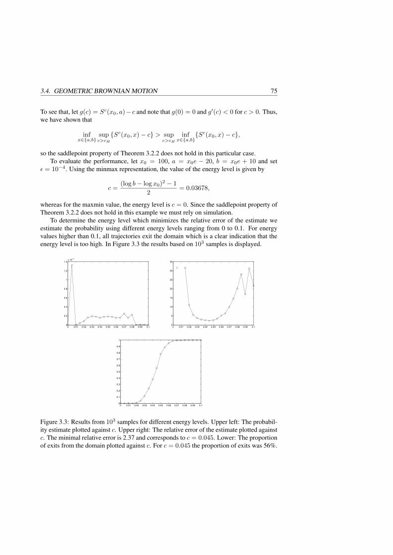
3.4. GEOMETRIC BROWNIAN MOTION 75
To see that, let g(c) = Sc(x0, a)− c and note that g(0) = 0 and g′(c) < 0 for c > 0. Thus,we have shown that
infx∈a,b
supc>cH
Sc(x0, x)− c > supc>cH
infx∈a,b
Sc(x0, x)− c,
so the saddlepoint property of Theorem 3.2.2 does not hold in this particular case.To evaluate the performance, let x0 = 100, a = x0e − 20, b = x0e + 10 and set
ε = 10−4. Using the minmax representation, the value of the energy level is given by
c =(log b− log x0)2 − 1
2= 0.03678,
whereas for the maxmin value, the energy level is c = 0. Since the saddlepoint property ofTheorem 3.2.2 does not hold in this example we must rely on simulation.
To determine the energy level which minimizes the relative error of the estimate weestimate the probability using different energy levels ranging from 0 to 0.1. For energyvalues higher than 0.1, all trajectories exit the domain which is a clear indication that theenergy level is too high. In Figure 3.3 the results based on 103 samples is displayed.
0 0.01 0.02 0.03 0.04 0.05 0.06 0.07 0.08 0.09 0.10
0.2
0.4
0.6
0.8
1
1.2
1.4x 10
−4
0 0.01 0.02 0.03 0.04 0.05 0.06 0.07 0.08 0.09 0.10
5
10
15
20
25
30
35
0 0.01 0.02 0.03 0.04 0.05 0.06 0.07 0.08 0.09 0.10
0.1
0.2
0.3
0.4
0.5
0.6
0.7
0.8
0.9
1
Figure 3.3: Results from 103 samples for different energy levels. Upper left: The probabil-ity estimate plotted against c. Upper right: The relative error of the estimate plotted againstc. The minimal relative error is 2.37 and corresponds to c = 0.045. Lower: The proportionof exits from the domain plotted against c. For c = 0.045 the proportion of exits was 56%.

76 CHAPTER 3. IMPORTANCE SAMPLING FOR DIFFUSIONS
From the upper left figure, we see that when c is close to zero there are no exits andthe probability estimate is therefore zero. The high estimate for c = 0.005 is the resultof one trajectory exiting the domain. The upper right figure shows the relative error ofthe estimate plotted against the energy level c. The minimal relative error corresponds toc = 0.045. The corresponding probability estimate is 1.77 · 10−5 and the proportion ofexits from the domain is 56%. Based on these finding we set c = 0.045 and perform alarger simulation study based on 105 samples for various values of ε. From the findingsillustrated in Figure 3.2 we know that c(ε) is stable for different values of ε. Thus, we willuse the same value of c for different values of ε. The results are displayed in Table 3.2.
Table 3.2: Probability estimates for Ω = (251.8, 281.8) and T = 1 for the geometricBrownian motion with drift. The energy level is c = 0.045.
ε Est. Rel. err. Var. red.5 · 10−4 3.11 · 10−2 1.51 13.34 · 10−4 1.87 · 10−2 1.59 20.63 · 10−4 8.19 · 10−3 1.72 41.02 · 10−4 1.65 · 10−3 1.93 172.81 · 10−4 1.69 · 10−5 2.42 8512.7
The numerical results based on the geometric Brownian motion indicate that the im-portance sampling algorithm yields significant variance reduction compared to standardMonte-Carlo simulation. In the first example, the saddlepoint property of Theorem 3.2.2could be verified so in that particular case the algorithm is asymptotically optimal and theresults in Table 3.1 verify that the algorithm works well in practice.
In the second example, we showed that the infimum and the supremum could not beinterchanged. However, by performing simulations for a range of energy levels, we coulddetermine the energy level which produced the smallest relative error. Using that energylevel, we conducted a larger simulation study for different values of ε. The results inTable 3.2 show that the algorithm outperforms standard Monte-Carlo even for fairly largeprobabilities.
3.5 The Cox-Ingersoll-Ross process
Suppose that Xε evolves according to the stochastic differential equation
dXε(t) = κ(θ −Xε(t))dt+√εσ√Xε(t)dB(t), Xε(0) = x0.
This process is called a Cox-Ingersoll-Ross process and was introduced in [2] to modelthe dynamics of interest rates. The same process is used in the Heston model, see [11],to model the volatility dynamics of the stock price. The popularity of the Cox-Ingersoll-Ross in mathematical finance is mainly due to two reasons. Firstly, the process is mean-reverting around its long run mean θ and the rate of the mean reversion is determined bythe parameter κ. Secondly, the square root in the diffusion coefficient guarantees that the

3.5. THE COX-INGERSOLL-ROSS PROCESS 77
process is nonnegative. In addition, if the Feller condition 2κθ ≥ σ2 is satisfied, the valuezero is excluded and the process is strictly positive, see [8].
With b(x) = κ(θ − x) and σ(x) = σ√x the Mañé potential (3.11) becomes
Sc(x0, x) =1
σ2
(κ(x− x0)− κθ(log x− log x0)
+ sign(x− x0)
∫ x
x0
√κ2(z − θ)2 + 2cσ2z
zdz),
(3.15)
where the last integral is given by
∫ x
x0
√κ2(z − θ)2 + 2cσ2z
zdz =
[ 1
κ
(κf(z)− cσ2 log
κ(f(z) + κ(θ − z)
)− cσ2
− κ2θ logκθf(z) + cσ2z + κ2θ(θ − z)
+ κ2θ log(z)
+ κ2θ logκ(f(z) + κ(θ − z)
)− cσ2
)]xx0
,
and f(z) =√κ2(z − θ)2 + 2cσ2z. Similarly, the gradient of the Mañé potential (3.12)
for the Cox-Ingersoll-Ross model becomes
DSc(x0, x) = −κ(θ − x)
σ2x+ sign(x− x0)
√κ2(x− θ)2 + 2cσ2x
σ2x,
so inserting this in the Girsanov kernel θ(t, x) = σ(x)DSc(x0, x) yields
θ(t, x) = −κ(θ − x)
σ√x
+ sign(x− x0)
√κ2(x− θ)2 + 2cσ2x
σ√x
.
To perform efficient importance sampling it remains to determine the asymptoticallyoptimal energy level c?. The expression for the Mañé potential in the Cox-Ingersoll-Rossmodel is more complicated than for geometric Brownian motion, but the fact that it canbe computed explicitly is important to determine the value of c at which the system issimulated. From the expression in (3.15) it should be obvious that verifying the saddlepointproperty (3.10) analytically is difficult. However, given a set of parameters the equationcan be verified numerically. In the following two examples we show how this is done.
Example 3.5.1 (A symmetric example). Let κ = 1, θ = 0.3, σ = 0.1, x0 = 0.3, T = 1/12and suppose that Ω = (a, b) where a = x0−R and b = x0 +R,R = 0.03. Note that in theCox-Ingersoll-Ross model, Mañé’s critical value is cH = 0 so if we can verify equation(3.10) the algorithm is asymptotically optimal.
Given the parameter values, for every c > cH it holds that Sc(x0, b) < Sc(x0, a), seeFigure 3.4, and it follows that
supc>cH
infx∈a,b
Sc(x0, x)− cT = supc>0Sc(x0, b)− cT.

78 CHAPTER 3. IMPORTANCE SAMPLING FOR DIFFUSIONS
Performing the optimization yields
supc>cH
infx∈a,b
Sc(x0, x)− cT = 1.8598. (3.16)
0 5 10 15 20 25 30 35 40 45 500
1
2
3
4
5
6
Figure 3.4: The Mañé potential Sc(x0, x) as a function of c for the Cox-Ingersoll processwith the parameters specified in Example 3.5.1. The red line corresponds to x = b and theblack corresponds to x = a.
The left-hand side of (3.10) can be computed as
infx∈a,b
supc>cH
Sc(x0, x)− cT = supc>0Sc(x0, a)− cT ∧ sup
c>0Sc(x0, b)− cT.
The supremum can be computed numerically and we find that
infx∈a,b
supc>cH
Sc(x0, x)− cT = 1.8598,
which coincides with the value in (3.16). Thus, the saddlepoint property of Theorem 3.2.2holds and we conclude that the importance sampling algorithm is asymptotically optimal.In particular, the asymptotically optimal energy level can be computed numerically and wefind that c? = 20.54.
In Table 3.3 numerical results are displayed when the diffusion parameter ε varies from0.2 to 0.6. Similar to the previous examples we choose ε to obtain probabilities in therange 10−2 to 10−5. The probability estimates are based on 105 samples and the timediscretization is T · 10−2.
In this example, the Mañé potential evaluated at a is almost equal to the Mañé potentialevaluated at b. The interpretation is that the dynamics of Xε are such that the process isalmost as likely to exit the domain through a as through b. In these situations, where thedomain is symmetric about x0, the importance sampling performs very well compared tostandard Monte-Carlo simulation. In the following example, we discuss how an asymmet-ric domain affects the performance.

3.5. THE COX-INGERSOLL-ROSS PROCESS 79
Table 3.3: Probability estimates for Ω = (0.27, 0.33) and T = 1/12 in the Cox-Ingersoll-Ross model. The asymptotically optimal energy level is c? = 20.54.
ε Est. Rel. err. Var. red.0.6 1.46 · 10−2 2.48 14.40.4 2.78 · 10−3 2.66 88.20.3 5.76 · 10−4 3.25 270.10.2 2.60 · 10−5 4.42 5116.7
Example 3.5.2 (An asymmetric example). Consider the same parameter values as in theprevious example, but suppose that Ω = (a, b) with a = x0 − 2R and b = x0 + R,R = 0.03. Then Sc(x0, b) < Sc(x0, a) for every c > 0 so the optimal energy level is thesame as in the previous example, c? = 20.54. In Table 3.4 numerical results are displayedwhen the parameter ε varies from 0.2 to 0.8. The estimates are based on 105 samples andthe step size in the time discretization is T · 10−2.
Table 3.4: Probability estimates for Ω = (0.24, 0.33) and T = 1/12 in the Cox-Ingersoll-Ross model. The asymptotically optimal energy level is c? = 20.54.
ε Est. Rel. err. Var. red.0.8 1.90 · 10−2 3.15 6.60.6 8.29 · 10−3 3.55 12.70.4 1.71 · 10−3 3.77 60.60.3 3.71 · 10−4 4.52 408.00.2 1.76 · 10−5 4.77 4399.4
If we compare the relative errors in the symmetric example, see Table 3.3, with therelative errors in the asymmetric example, see Table 3.4, we see that for a fixed probabilitythe relative error is higher for the asymmetric problem. This is particularly apparent inFigure 3.5, where the relative error is plotted against the corresponding probability esti-mate. Obviously, the performance of the algorithm is affected negatively when the domainis asymmetric about the initial state x0.
In the asymmetric case, the cost of going from x0 to b is lower than going from x0 toa which is why Sc(x0, b) < Sc(x0, a). Therefore, the energy level c is based on Sc(x0, b)and this energy level is lower than the energy level based on Sc(x0, a). Consequently, tra-jectories moving from x0 towards a are unlikely to exit from the domain and the proportionof exits from the domain decreases from about 50% in the symmetric case to about 25%in the asymmetric case. Thus, the loss in performance is caused by a decrease of exitingtrajectories under the sampling measure.
Acknowledgements
We are grateful to Filip Lindskog for discussions and comments that helped us to improvethe manuscript. Henrik Hult’s research is supported by the Swedish Research Council.

80 CHAPTER 3. IMPORTANCE SAMPLING FOR DIFFUSIONS
0 0.01 0.02 0.03 0.04 0.05 0.061.5
2
2.5
3
3.5
4
4.5
5
Figure 3.5: The relative error (y-axis) plotted against the probability estimate (x-axis)based on the importance sampling simulation. The red line corresponds to the asymmetricdomain and the black line corresponds to the symmetric case.
3.6 References
[1] F. Black and M. Scholes (1973), The pricing of options and corporate liabilities,Journal of Political Economy, 81(3), 637-654.
[2] J. C. Cox, J. E. Ingersoll and S. A. Ross (1985), A theory of the term structure ofinterest rates, Econometrica, 53, 385-407.
[3] B. Djehiche, H. Hult and P. Nyquist (2014), Min-max representations of viscositysolutions of Hamilton-Jacobi equations and applications in rare-event simulation.Preprint.
[4] P. Dupuis, K. Spiliopoulos and H. Wang (2012), Importance sampling for multiscalediffusions. Multiscale Modeling & Simulation, 10, 1-27.
[5] P. Dupuis, K. Spiliopoulos, and X. Zhou (2013), Escaping from an attractor: Impor-tance sampling and rest points I. Preprint.
[6] P. Dupuis and H. Wang (2007), Subsolutions of an Isaacs equation and efficientschemes for importance sampling. Mathematics of Operations Research, 32(3), 723-757.
[7] C. Evans, Partial Differential Equations, second edition, American MathematicalSociety, 2010.
[8] W. Feller (1951), Two singular diffusion problems, Annals of Mathematics, 54, 173-182.
[9] J. Feng and T. G. Kurtz, Large deviations for stochastic processes, American Math-ematical Society, 2006.

3.6. REFERENCES 81
[10] M. I. Freidlin and A. D. Wentzell, Random perturbations of dynamical systems,Springer, 1984.
[11] S. L. Heston (1993), A closed-form solution for options with stochastic volatilitywith applications to bond and currency options, Review of Financial Studies, 6(2),327-343.
[12] P. Guasoni and S. Robertson (2008), Optimal importance sampling with explicitformulas in continuous time, Finance and Stochastics, 12, 1-19.
[13] I. Karatzas and S. E. Shreve, Brownian Motion and Stochastic Calculus, secondedition, Springer, 1991.
[14] E. Vanden-Eijnden and J. Weare (2012), Rare event simulation for small noise dif-fusions, Communications in Pure and Applied Mathematics 65(12), 1770.1803.


Chapter 4
83

Efficient importance samplingto compute loss probabilities
in financial portfolios
by
Henrik Hult and Johan Nykvist
Abstract
In this paper we construct an efficient importance sampling algorithm for comput-ing the probability that a portfolio of financial derivatives suffers a large loss over afixed time horizon. The derivatives may be path-dependent and we consider the multi-dimensional Black-Scholes model as well as the Heston model for the evolution ofthe underlying asset prices. The change of measure used for importance sampling isexpressed in terms of a subsolution to a Hamilton-Jacobi equation associated with thelarge deviations of underlying price process. The construction of the subsolution isfacilitated by a minmax representation of viscosity solutions of the Hamilton-Jacobiequation that involves the Mañé potential. A particular feature of the proposed methodis that the composition of the portfolio only enters the design of the change of measurethrough a parameter c that can be physically interpreted as the energy level of the sys-tem. This makes the proposed class of algorithms robust across portfolios but comesat the cost of potential reduction of performance. The performance of the importancesampling algorithms is investigated through numerical experiments for a wide range ofderivative portfolios.
4.1 Introduction
Consider a portfolio consisting of positions of financial derivatives written on liquidlytraded financial assets. It is assumed that the derivatives, which may be path-dependent,can be accurately priced, at least numerically. To quantify the risk of the portfolio it is ofinterest to compute the probability of a significant portfolio loss over a finite time horizon.The profit-and-loss distribution is typically inaccessible and it is therefore often necessaryto resort to stochastic simulation for the estimation of loss probabilities.
When extreme losses are considered the sought probability is small, say of the order10−3 to 10−5, and standard Monte Carlo simulation is inefficient because a large sample
85

86 CHAPTER 4. IMPORTANCE SAMPLING FOR LOSS PROBABILITIES
size is needed to obtain accurate estimates. If the portfolio is large and prices of some ofthe derivatives must be computed numerically the evaluation of the portfolio loss is nu-merically costly, which limits the number of scenarios that can be generated and evaluatedwithin a given time frame.
Importance sampling has become a popular method to reduce the variance of the esti-mator and thereby lowering the computational cost. In importance sampling the underlyingprice process is simulated under a sampling measure, under which large portfolio lossesare more likely to occur, and the probability is estimated as the sample mean of the likeli-hood ratios of the scenarios that lead to large portfolio losses. However, the design of thesampling measure is delicate; a good choice may reduce the computational cost by severalorders of magnitude whereas a poor choice may lead to a performance that is worse thanstandard Monte Carlo.
In the context of portfolio risk management importance sampling techniques for com-puting loss probabilities have been developed and popularized by Glasserman and his col-laborators, see e.g. [15, 2] and the references therein. In [16] an importance samplingalgorithm is developed in a one period log-normal setting for computing loss probabilitiesof a portfolio of European derivatives. There the change of measure is based on the delta-gamma approximation of the portfolio. This technique can also be applied to computerisk measures, such as Value-at-Risk, see [17]. Dynamic importance sampling for pricingexotic path-dependent options in a Black-Scholes model are developed in [18].
This paper studies importance sampling algorithms for computing the probability thata derivative portfolio suffers a large loss within a finite time horizon, T > 0. This problemis conveniently formulated as the probability that a diffusion is outside a domain at time T .Let Xε be the unique strong solution, on an underlying probability space (ℵ,A,P), to thestochastic differential equation
dXε(t) = b(Xε(t))dt+√εσ(Xε(t))dB(t), Xε(0) = x0, (4.1)
where b, σ are smooth and bounded functions and B is a Brownian motion. Xε(t) ∈ Rn
represents the prices of underlying financial assets and possibly additional information,e.g. volatility, that determines the prices of the derivatives. For any given portfolio ofderivatives it is assumed that there is a continuous pricing function FT : Rn → R suchthat the value of the portfolio at time T is given by FT (Xε(T )). Let A = x ∈ Rn :FT (x) ≤ v0 be the set of states where the portfolio value falls below a given lowerthreshold v0 at time T . We will be concerned with importance sampling algorithms forcomputing PXε(T ) ∈ A.
From the rare-event simulation perspective the problem to compute exit probabilitiesfor diffusions by importance sampling is reasonably well studied, see e.g. [18, 23, 9]. Inimportance sampling the process Xε is sampled from the sampling measure Qε, with PQε on the set Xε(T ) ∈ A, and an estimator for pε = PXε(T ) ∈ A is constructed asthe sample average of independent replicates of
pε = IXε(T ) ∈ A dP
dQε(Xε). (4.2)

4.1. INTRODUCTION 87
For the diffusion model considered here the change of measure is naturally given byGirsanov’s theorem, through the Girsanov kernel θ as
dQε
dP= exp
− 1
2ε
∫ T
0
|θ(t,Xε(t))|2dt+1√ε
∫ T
0
〈θ(t,Xε(t)), dB(t)〉
and the corresponding dynamics under Qε is given by
dXε(t) =(b(Xε(t)) + σ(Xε(t))θ(t,Xε(t))
)dt+
√εσ(Xε(t))dBε(t), Xε(0) = x0,
where Bε is a Qε-Brownian motion. The general heuristic is that the change of measure,in terms of the Girsanov kernel θ, should be chosen such that the process tends to followthe most likely path to exit. Typically, large deviation asymptotics are used to identify themost likely path to exit. A difficulty in the present case is that the boundary of the set,∂A, may be numerically costly to compute, in particular if the portfolio consists of a largenumber of derivatives and the pricing function FT can only be evaluated numerically.
In this paper the subsolution approach by Dupuis and Wang [10] is employed, wherethe choice of the Girsanov kernel, θ, is connected to the construction of classical subsolu-tions to an associated partial differential equation of Hamilton-Jacobi type. More precisely,under suitable conditions on the drift b and the diffusion coefficient σ, the large deviationsrate U(t, x) = limε→0 ε log PXε(T ) ∈ A | Xε(t) = x is the unique continuous viscos-ity solution to the Hamilton-Jacobi equation
Ut(t, x)−H(x,−DU(t, x)) = 0, (t, x) ∈ (0, T )×Rn,
U(T, x) = 0, x ∈ A,U(T, x) =∞, x /∈ A,
where Ut and DU denotes the time derivative and gradient of U , respectively. If a piece-wise classical subsolution U of the Hamilton-Jacobi equation can be constructed, suchthat U(0, x0) = U(0, x0), then the importance sampling estimator obtained by takingθ(t, x) = −σT (x)DU(t, x) is asymptotically optimal.
The subsolutions considered here are constructed from the Mañé potential as suggestedin [6]. More precisely, U takes the form
U(t, x) = constant− Sc(x0, x)− c(T − t),
where Sc is the Mañé potential at level c. That is, for each x, y 7→ Sc(x, y) is the maximalviscosity subsolution to the stationary Hamilton-Jacobi equation H(y,DSc(x, y)) = c.Here c can be interpreted as the energy level at which the system is simulated. The detailsare presented in Section 4.3.2 below. The advantage of this approach is that the Girsanovkernel θ(t, x) = −σT (x)DU(t, x) = σT (x)DSc(x0, x) does not depend on t and onlydepends on the set A through the choice of the energy level c at which to simulate thesystem. Therefore, quantities such as the most likely point of exit on the boundary of A donot have to be computed.

88 CHAPTER 4. IMPORTANCE SAMPLING FOR LOSS PROBABILITIES
The contributions of this paper can be summarized as follows. Using the method ofcharacteristics, the Mañé potential is computed explicitly for a multi-dimensional Black-Scholes model. The corresponding importance sampling algorithm is implemented to com-pute loss probabilities for various derivative portfolios. A particular feature of the subso-lutions based on the Mañé potential is that the composition of the portfolio and the corre-sponding pricing function FT only enters the design of the change of measure through thechoice of the energy level c. This implies a certain robustness of the proposed method, butalso that the algorithms are by no means optimal for any given portfolio. On the contrary, itis relatively easy to construct portfolios where a more delicate design outperforms the pro-posed method. On the other hand, the proposed method is applicable for a wide range ofportfolios and performs consistently well. For example, as will be evident from the numer-ical experiments in Section 4.4, the method based on the Mañé potential is outperformedby the delta-gamma method of [16], sometimes by a great deal, for 9 out of the 10 port-folios of European derivatives studied in [16]. However, for the delta-hedged portfolio themethod based on the Mañé potential performs better. For delta-gamma neutral portfoliosthe delta-gamma approach is not even applicable whereas the method based on the Mañépotential displays good performance. In addition, the delta-gamma approach does not al-low for path-dependent options whereas the method based on the Mañé potential performswell also in this setting. In addition, it is shown, using the method of characteristics, thatthe gradient of the Mañé potential can be evaluated numerically for the Heston model andthe importance sampling algorithm for the Heston model is implemented to compute lossprobabilities for a portfolio consisting of a delta-hedged European call option.
The paper is organized as follows. In Section 4.2 the importance sampling techniquebased on the delta-gamma approximation, proposed in [16, 17] is briefly reviewed. Thesubsolution approach to efficient importance sampling and the general construction of sub-solutions based on the Mañé potential is presented in Section 4.3. The Mañé potential isexplicitly computed for the multi-dimensional Black-Scholes model in Section 4.4 wherenumerical experiments displaying the performance of the method is illustrated. Finally, inSection 4.5, the Heston model is considered and it is shown how the gradient of the Mañépotential can be evaluated numerically using the method of characteristics. The numericalperformance of the corresponding importance sampling algorithms is also demonstrated.
4.2 The Delta-Gamma approximation and importance sampling
In [16, 17] an importance sampling algorithm is developed in a one-period setting wherethe risk factors have a multivariate normal distribution. Thus, the algorithm can be usedin the Black-Scholes model for estimating loss probabilities of portfolios containing Euro-pean derivatives. In Section 4.4.3 we compare the importance sampling scheme in [16] tothe method derived in this paper. For clarity, we give a brief summary of their work andfor further details we refer to the original paper [16].
Suppose the current value of the portfolio is V (t), the holding period has length ∆t andthat the lossL over the time interval [t, t+∆t] is defined byL = −∆V = V (t)−V (t+∆t).The task is to compute PL > x, the probability that the loss exceeds some threshold x.

4.2. THE DELTA-GAMMA APPROXIMATION 89
We assume that there are n risk factors, and that S(t) = (S1(t), . . . , Sn(t)) denotes thevalue of these factors at time t. Define ∆S = [S(t+ ∆t)− S(t)]T to be the change in therisk factors during the interval [t, t + ∆t] and suppose that ∆S has a multivariate normaldistribution with mean zero and covariance matrix Σ. To sample from ∆S, let ∆S = CZ,where Z has a standard multivariate normal distribution and C is any matrix satisfyingCCT = Σ.
The sampling distribution for Z is constructed through an exponential change of mea-sure, see [15, Example 4.6.2], where the mean and the covariance matrix are changed fromzero to µθ and from I to Bθ, respectively. Then,
PL > x = E[IL > xl(Z)], (4.3)
where the expectation is taken under the sampling measure and l(Z) is the likelihood ratio.The parameters µθ and Bθ are based on the delta and the gamma of the portfolio.
The delta-gamma approximation is given by
∆V = −L ≈ Θ∆t+ δT∆S +1
2∆STΓ∆S,
where Θ = ∂V∂t , δi = ∂V
∂Siand Γij = ∂2V
∂Si∂Sj. Following [16] we can write
L ≈ −Θ∆t+ bTZ + ZTΛZ,
where b = −CT δ, Λ = − 12C
TΓC and C is a matrix satisfying
CCT = Σ and1
2CTΓC is diagonal.
Thus,
PL > x ≈ PQ > yx,
whereQ = bTZ+ZTΛZ and yx = x+Θ∆t. The probability PL > x is approximatedby PQ > yx and the importance sampling algorithm is therefore designed to increasethe probability of the event Q > yx under the sampling measure.
Let θ be a real number and define
Bθ = (I − 2θΛ)−1 and µθ = θBθb.
Then, the likelihood ratio in (4.3) can be computed as
l(Z) = exp−θQ+ ψ(θ), (4.4)
where ψ is given by
ψ(θ) =1
2
n∑
i=1
( (θbi)2
1− 2θλi− log(1− 2θλi)
).

90 CHAPTER 4. IMPORTANCE SAMPLING FOR LOSS PROBABILITIES
In particular, if θ is chosen as the unique solution to the nonlinear equation ψ′(θ) = yx,then the mean of Q under the sampling measure is equal to yx.
The performance of the importance sampling algorithm in [16] is analyzed for a varietyof portfolios consisting of European put and call options. Since the relevant magnitudeof losses varies widely across models, the loss threshold x is specified as xstd standarddeviations above the mean loss according to the delta-gamma approximation:
x =( n∑
i=1
λi −Θ∆t)
+ xstd
√√√√n∑
i=1
(b2i + 2λ2
i
). (4.5)
In Section 4.4.3 we use the portfolios considered in [16] to investigate the performance ofthe algorithm proposed in Section 4.4. Firstly, we discuss importance sampling algorithmsfor stochastic processes and the connection to partial differential equations of Hamilton-Jacobi type.
4.3 Importance sampling and Hamilton-Jacobi equations
In this section the importance sampling methodology for computing rare events will bedescribed in some detail. The construction of the importance sampling algorithm that wepropose in this paper is based on the subsolution approach by Dupuis and Wang, see [10],where the subsolutions are constructed from the Mañé potential, as suggested in [6].
4.3.1 The subsolution approach to efficient importance sampling
Consider a collection of n-dimensional diffusion processes Xε(t); t ∈ [0,∞)ε>0 suchthat, for each ε > 0, Xε is the unique strong solution to the stochastic differential equation
dXε(t) = b(Xε(t))dt+√εσ(Xε(t))dB(t), Xε(0) = x0, (4.6)
where B is an n-dimensional Brownian motion and b, σ are Lipschitz continuous andsatisfies appropriate growth conditions so that a strong solution exists, see [21]. Let A ⊆Rn be a closed set and T > 0. The task is to compute pε = PXε(T ) ∈ A.
The importance sampling estimator for pε is constructed as the sample average of in-dependent replicates of
pε = IXε(T ) ∈ A dP
dQε(Xε),
where Xε is simulated under the sampling measure Qε and P Qε on the set Xε(T ) ∈A so that, by the Radon-Nikodym theorem, the likelihood ratio exists. The estimator pεis unbiased because
EQε [pε] = EP[IXε(T ) ∈ A] = pε.

4.3. IMPORTANCE SAMPLING AND HAMILTON-JACOBI EQUATIONS 91
Therefore, the performance of the estimator can be evaluated in terms of its variance:
VarQε(pε) = EQε[IXε(T ) ∈ A2
( dP
dQε
)2]− EQε
[IXε(T ) ∈ A dP
dQε
]2
= EQε[IXε(T ) ∈ A
( dP
dQε
)2]− p2
ε .
The second term does not depend on Qε so it suffices to consider the second moment ofthe estimator. The idea behind efficient importance sampling is to choose a practicallyimplementable sampling measure Qε that gives controlled second moment, relative to p2
ε .Suppose that, as ε→ 0, the probability pε decays exponentially in ε:
limε→0−ε log pε = γ, (4.7)
where γ is the exponential rate of decay. From Jensen’s inequality it follows that a simplelower bound on the second moment is given by
EQε[IXε(T ) ∈ A2
( dP
dQε
)2]≥ EQε
[IXε(T ) ∈ A dP
dQε
]2= p2
ε .
Then (4.7) gives the asymptotic upper bound
lim supε→0
−ε log EQε[IXε(T ) ∈ A
( dP
dQε
)2]≤ 2γ.
If the sampling measure Qε satisfies the corresponding lower bound, that is, if
lim infε→0
−ε log EQε[IXε(T ) ∈ A
( dP
dQε
)2]≥ 2γ, (4.8)
then Qε is said to be asymptotically optimal, see [10]. The aim is to find an asymptoticallyoptimal sampling measure Qε.
The subsolution approach of Dupuis and Wang [10] is a useful method to design andanalyze sampling measures. Before going into its details, let us make some simplifyingassumptions on the stochastic model in (4.6) under which the diffusion, Xε, satisfies alarge deviation principle of the form (4.7). The assumptions are stronger than necessaryand can be weakened.
Condition 4.3.1. (i) The drift b is bounded and Lipschitz continuous.
(ii) The diffusion coefficient σ is bounded, Lipschitz continuous and uniformly nonde-generate.
Under Condition 4.3.1 the large deviations rate is given as the value of a variationalproblem:
γ = inf∫ T
0
L(ψ(s), ψ(s))ds;ψ ∈ AC([0, T ];Rn), ψ(0) = x0, ψ(T ) ∈ A,

92 CHAPTER 4. IMPORTANCE SAMPLING FOR LOSS PROBABILITIES
where AC([0, T ];Rn) denotes the set of all absolutely continuous functions ψ : [0, T ] →Rn, see e.g. [9, 8, 14]. The function L is called the local rate function and can be writtenas
L(x, v) =1
2|σ−1(x)(v − b(x))|2.
Let the function U(t, x) be defined by
U(t, x) = inf∫ T
t
L(ψ(t), ψ(t))dt;ψ ∈ AC([t, T ];Rn), ψ(t) = x, ψ(T ) ∈ A.
It is well known, see e.g. [11, Chapter 10], that U is the unique continuous viscositysolution to the Hamilton-Jacobi equation
Ut(t, x)−H(x,−DU(t, x)) = 0, (t, x) ∈ (0, T )×Rn,
U(T, x) = 0, x ∈ A,U(T, x) =∞, x /∈ A,
(4.9)
where Ut denotes the time derivative and DU the gradient of U . The Hamiltonian H isgiven by the Fenchel-Legendre transform of L,
H(x, p) = supv
〈p, v〉 − L(x, v)
= 〈b(x), p〉+
1
2|σT (x)p|2. (4.10)
From the work of [8, 9] it follows that an asymptotically optimal sampling measurecan be constructed from a classical (or piecewise classical) subsolution to the Hamilton-Jacobi equation (4.9). More precisely, suppose U is a piecewise continuously differentiablefunction that satisfies
Ut(t, x)−H(x,−DU(t, x)) ≥ 0, (t, x) ∈ (0, T )×Rn,
U(T, x) ≤ 0, x ∈ A. (4.11)
Define Qε by
dQε
dP= exp
− 1
2ε
∫ T
0
|θ(t,Xε(t))|2dt+1√ε
∫ T
0
〈θ(t,Xε(t)), dB(t)〉,
where θ(t, x) = −σT (x)DU(t, x).
Theorem 4.3.1 ([8], Theorem 4.1). Suppose that Condition 4.3.1 holds, θ is bounded, Usatisfies (4.9) and U satisfies (4.11). Then
lim infε→0
−ε log EQε[Iτ ε ≤ T
( dP
dQε
)2]≥ U(0, x0) + U(0, x0). (4.12)

4.3. IMPORTANCE SAMPLING AND HAMILTON-JACOBI EQUATIONS 93
From Theorem 4.3.1 it follows that the performance of pε, as measured by the expo-nential decay of the second moment, is determined by the initial value of the subsolution.In particular, suppose that U(0, x0) = U(0, x0). Then the right-hand side of (4.12) is equalto 2U(0, x0) and from the variational formulation of U(t, x) it follows that U(0, x0) = γ.Thus, the right-hand side of (4.12) equals 2γ so the asymptotic lower bound (4.8) is sat-isfied. Therefore, the sampling measure Qε based on U is asymptotically optimal. In thefollowing subsection we will present a construction of appropriate subsolutions based onthe Mañé potential.
4.3.2 Construction of subsolutions based on the Mañé potential
For c ∈ R and x, y ∈ Rn the Mañé potential at level c, denoted by Sc(x, y), is defined as
Sc(x, y)
= inf∫ τ
0
(c+ L(ψ(s), ψ(s))
)ds, ψ ∈ AC([0,∞);Rn), ψ(0) = x, ψ(τ) = y, τ > 0
.
Whenever it is finite, the function y 7→ Sc(x, y) is a viscosity subsolution of the stationaryHamilton-Jacobi equation
H(y,DSc(x, y)) = c, y ∈ Rn. (4.13)
It is a viscosity solution to (4.13) on Rn \ x, see e.g. [6] and the references therein.Let cH denote Mañé’s critical value; the infimum over c ∈ R for which the stationary
Hamilton-Jacobi equation (4.13) admits a global viscosity subsolution. For the Hamilto-nian H given in (4.10) Mañé’s critical value is given by cH = − 1
2 infx |b(x)|2, see [6],Example 2.1.
The function U can be given the following minmax representation:
U(t, x) = infy∈∂A
supc>cH
Sc(x, y)− c(T − t),
see [6], Proposition 3.3.It may be difficult to compute U(t, x) and DU(t, x) because for each (t, x) one needs
to optimize over c > cH and y ∈ ∂A. This is particularly difficult when the boundary ∂A isnot given explicitly. A construction of subsolutions, based on the minmax representation,that is useful for importance sampling is given below.
For c > cH and y ∈ ∂A, consider the collection of functions U c,y(·, ·) defined by
U c,y(t, x) = Sc(x0, y)− Sc(x0, x)− c(T − t). (4.14)
If x 7→ Sc(x0, x) is continuously differentiable on Rn \ x0, then, for 0 ≤ t ≤ T andx 6= x0,
U c,yt (t, x)−H(x,−DU c,y(t, x)) = c−H(x,DSc(x0, x)) = 0.

94 CHAPTER 4. IMPORTANCE SAMPLING FOR LOSS PROBABILITIES
Since the Mañé potential is viscosity subsolution of the stationary Hamilton-Jacobi equa-tion (4.13), the last equality is an inequality (≥) when x = x0, so U c,y is a subsolutionto the evolutionary equation: U c,yt (t, x) − H(x,−DU c,y(t, x)) ≥ 0. To verify (4.11) itremains to check the boundary condition. If the boundary condition is not satisfied one cansimply substract a positive constant from U c,y that is sufficiently large so that the bound-ary condition is satisfied. However, the same constant appears in the initial value of thesubsolution, which implies that the resulting estimator will not be asymptotically optimal.It turns out that the efficiency of the importance sampling estimator based on U c,y relieson a saddlepoint property, as the following result demonstrates.
Theorem 4.3.2 (c.f. [6], Proposition 5.1). If
infy∈∂A
supc>cH
Sc(x0, y)− cT = supc>cH
infy∈∂A
Sc(x0, y)− cT, (4.15)
then U c,y , given by (4.14), satisfies (4.11) in the viscosity sense and U c,y(0, x0) = U(0, x0).
The discussion above provides the necessary tools for finding an asymptotically opti-mal sampling measure Qε. Indeed, if x 7→ Sc(x0, x) is piecewise continuously differen-tiable and the saddlepoint property (4.15) holds then, with (c, y) defining the saddlepoint,an asymptotically optimal importance sampling estimator is given by
pε = IXε(T ) ∈ A dP
dQε(Xε),
where Xε is sampled from Qε,
dQε
dP= exp
− 1
2ε
∫ T
0
|θ(Xε(t))|2dt+1√ε
∫ T
0
〈θ(Xε(t)), dB(t)〉,
with
θ(x) = −σT (x)DU c,y(t, x) = σT (x)DSc(x0, x).
It is remarkable that the boundary of the set, ∂A, only enters the design through the choiceof the energy level c defining the saddlepoint.
4.4 Importance sampling in the n-dimensional Black-Scholes model
In this section we construct an importance sampling algorithm for rare-event simulationin the Black-Scholes model, see [4]. Using the method of characteristics we compute anexplicit expression for the Mañé potential and its gradient. Four numerical experiments areprovided to illustrate the efficiency of the method.
Consider the n-dimensional Black-Scholes model where the market consists of n riskyassets and the evolution of the spot prices is given by a multi-dimensional geometric Brow-nian motion:
dXεi (t) = µiX
εi (t)dt+
√εXε
i (t)
n∑
j=1
LijdBj(t), Xεi (0) = x0,i.

4.4. THE BLACK-SCHOLES MODEL 95
The matrix L specifies the dependence in the multivariate normal distribution of the log-returns:
(log (Xε
1(t+ h)/Xε1(t)), . . . , log (Xε
n(t+ h)/Xεn(t))
)T
has a normal distribution with mean (µ1h, . . . , µnh)T and covariance matrix εhLLT . Wewrite Σ = LLT and Σij = ρijγiγj . Then Xε(t) = (Xε
1(t), . . . , Xεn(t))T satisfies a
stochastic differential equation of the form (4.6), where the ith component of b(x) is µixiand element (i, j) of the matrix σ(x) is given by σij(x) = Lijxi. Let A ⊂ Rn be a closedset and fix the time T > 0. The task is to compute PXε(T ) ∈ A, the probability thatthe diffusion hits A at time T .
4.4.1 Computing the Mañé potential
In this section we use the method of characteristics to compute an explicit expression forthe Mañé potential and its gradient for the n-dimensional Black-Scholes model.
The Hamiltonian H associated with the stochastic process Xε is given by (4.10) soinserting the expressions for b(x) and σ(x) we obtain
H(x, p) =1
2
n∑
i=1
(2µipixi + γ2
i p2ix
2i +
∑
j 6=i
ρijγiγjpipjxixj
).
Thus, the stationary Hamilton-Jacobi equation (4.13) becomes
n∑
i=1
(2µipixi + γ2
i p2ix
2i +
∑
j 6=i
ρijγiγjpipjxixj
)− 2c = 0. (4.16)
For n = 1, the nonlinear first order partial differential equation (4.16) simplifies to aquadratic equation for p and the general solution is given by
p = ±√µ2 + 2cγ2
γ2x− µ
γ2x.
The Mañé potential is a primitive function of p and the maximal of all subsolutions vanish-ing at x0, see [6, Proposition 2.1(ii)]. Therefore, the± sign must be selected as sign(x−x0)and the Mañé potential becomes
Sc(x0, x) =sign(x− x0)
√µ2 + 2cγ2 − µγ2
log( xx0
).
For n > 1, (4.16) can be solved using the method of characteristics which solves(4.16) by converting the partial differential equation into an appropriate system of ordinarydifferential equations, see [11]. Assume that Sc solves (4.16) and fix any point x ∈ Rn.The idea is to calculate Sc(x0, x) by finding some curve connecting x with the point x0
and along which we can compute Sc. Since we know the value at the one end x0, we hopethen to be able to calculate Sc all along the curve, and so in particular at x.

96 CHAPTER 4. IMPORTANCE SAMPLING FOR LOSS PROBABILITIES
Suppose that the curve is described parametrically by the function ξ(t) = (ξ1(t), . . . ,ξn(t)), the parameter t lying in some subinterval 0 3 I ⊆ R, and ξ(0) = (x0,1, . . . , x0,n).In addition, let ζ(t) := Sc(x0, ξ(t)) and let π(t) := DSc(x0, ξ(t)). Then (4.16) canbe written F (π(t), ζ(t), ξ(t)) = 0, where F (π, ζ, ξ) = |σT (ξ)π|2 + 2〈b(ξ), π〉 − 2c.Following [11] the characteristic equations are given by
π(t) = −DξF (π(t), ζ(t), ξ(t))−DζF (π(t), ζ(t), ξ(t)),
ζ(t) = 〈Dπ(π(t), ζ(t), ξ(t)), π(t)〉,ξ(t) = DπF (π(t), ζ(t), ξ(t)).
(4.17)
To determine the characteristic equations we compute the partial derivatives of F withrespect to π, ζ and ξ, respectively, which yields
∂F
∂πi= 2(µi + γ2
i πiξi +∑
j 6=i
ρijγiγjπjξj
)ξi,
∂F
∂ζ= 0,
∂F
∂ξi= 2(µi + γ2
i πiξi +∑
j 6=i
ρijγiγjπjξj
)πi.
Inserting the expressions, the system of characteristic equations becomes
πi(t) = −2(µi + γ2
i πi(t)ξi(t) +∑
j 6=i
ρijγiγjπj(t)ξj(t))πi(t),
ζ(t) = 2
n∑
i=1
(µiπi(t)ξi(t) + γ2
i π2i (t)ξ2
i (t) +∑
j 6=i
ρijγiγjπi(t)πj(t)ξi(t)ξj(t)),
ξi(t) = 2(µi + γ2
i πi(t)ξi(t) +∑
j 6=i
ρijγiγjπj(t)ξj(t))ξi(t).
(4.18)
The solution to the system of ordinary differential equations is given by the followingtheorem.
Proposition 4.4.1. The solution to (4.18) is given by
πi(t) = πi(0) exp− 2(µi + γ2
i πi(0)x0,i +∑
j 6=i
ρijγiγjπj(0)x0,j
)t,
ζ(t) = 2
n∑
i=1
(µiπi(0)x0,i + γ2
i π2i (0)x2
0,i +∑
j 6=i
ρijγiγjπi(0)πj(0)x0,ix0,j
)t,
ξi(t) = x0,i exp
2(µi + γ2
i πi(0)x0,i +∑
j 6=i
ρijγiγjπj(0)x0,j
)t.

4.4. THE BLACK-SCHOLES MODEL 97
Proof. From the first and third equation of (4.18) it immediately follows that
d
dt
(πi(t)ξi(t)
)= πi(t)ξi(t) + πi(t)ξi(t) = 0,
from which we deduce that πi(t)ξi(t) = πi(0)x0,i. Using this, the equations in (4.18) canbe simplified and for πi(t) we get
πi(t) = −2(µi + γ2
i πi(0)x0,i +∑
j 6=i
ρijγiγjπj(0)x0,j
)πi(t).
This is a separable ordinary differential equation and the solution is given by
πi(t) = πi(0) exp− 2(µi + γ2
i πi(0)x0,i +∑
j 6=i
ρijγiγjπj(0)x0,j
)t.
From the relation between πi and ξi we immediately get the solution for ξi. Finally, theequation for ζ(t) is reduced to
ζ(t) = 2
n∑
i=1
(µiπi(0)x0,i + γ2
i π2i (0)x2
0,i +∑
j 6=i
ρijγiγjπj(0)πj(0)x0,ix0,j
),
which implies that ζ(t) is linear in t. Integrating both sides and using the fact that ζ(0) =Sc(x0, x0) = 0, see the definition of Sc in Section 4.3.2, yields the expression for ζ(t).This completes the proof.
For the purpose of performing efficient importance sampling we need to evaluate thegradient of the Mañé potential at the point x. By definition, ζ(t) = Sc(x0, ξ(t)) and π(t) =DSc(x0, ξ(t)) where both ζ and π depend on the unknown constants π1(0), . . . , πn(0).Thus, it remains to determine π1(0), . . . , πn(0).
Suppose that we want to compute Sc(x0, x). Since ζ(t) = Sc(x0, ξ(t)) we assume thatthere exists a real number tx such that ξ(tx) = x. From the third equation of Proposition4.4.1, it follows that the equation ξ(tx) = x can be written
x0,i exp
2(µi + γ2
i πi(0)x0,i +∑
j 6=i
ρijγiγjπj(0)x0,j
)tx
= xi,
or, equivalently,
γ2i πi(0)x0,i +
∑
j 6=i
ρijγiγjπj(0)x0,j =log xi − log x0,i
2tx− µi. (4.19)
For a given tx, (4.19) gives rise to a system of n linear equations for the n unknown con-stants π1(0), . . . , πn(0). To determine the appropriate value of tx, recall that the stationary

98 CHAPTER 4. IMPORTANCE SAMPLING FOR LOSS PROBABILITIES
Hamilton-Jacobi equation (4.16) takes the form F (π(t), ζ(t), ξ(t)) = 0 for all values of t.In particular, for t = 0 we get
n∑
i=1
(2µiπi(0)x0,i + γ2
i π2i (0)x2
0,i +∑
j 6=i
ρijγiγjπi(0)πj(0)x0,ix0,j
)= 2c. (4.20)
Thus, the equations in (4.19) and (4.20) yields a system of n + 1 equations for the n + 1variables π1(0), . . . , πn(0) and tx.
To solve for π1(0), . . . , πn(0) and tx, define zi = πi(0)x0,i and set li = log xi −log x0,i. With z = (z1, . . . , zn)T and l = (l1, . . . , ln)T equation (4.19) can be expressedon vector form as
Σz =l
2tx− µ,
so solving for z yields
z = Σ−1( l
2tx− µ
).
Similarly, equation (4.20) can be written on vector form as
zTΣz + 2µT z − 2c = 0.
Inserting the expression for z yields the following quadratic equation for tx:
lTΣ−1l
4t2x− µTΣ−1µ = 2c.
Solving for tx finally yields
tx = ±1
2
√lTΣ−1l
µTΣ−1µ+ 2c. (4.21)
From the expression for tx we can derive an explicit expression for the Mañé potentialSc(x0, x) evaluated at the point x. Recall that Sc(x0, x) = ζ(tx), so combining the secondequation of Proposition 4.4.1 with (4.21) yields
ζ(tx) = ±√µTΣ−1µ+ 2c
√lTΣ−1l − lTΣ−1µ.
Since the Mañé potential is the maximal of all subsolutions vanishing at x0 the ± signmust be selected as positive. Thus, the Mañé potential is given by
Sc(x0, x) =√µTΣ−1µ+ 2c
√lTΣ−1l − TΣ−1µ.
Similarly, by the definition of π we know that DSc(x0, x) = π(tx). Then π(tx) =diag(x)−1z so using the expression for z we obtain
DSc(x0, x) = diag(x)−1Σ−1(√µTΣ−1µ+ 2c
lTΣ−1ll − µ
).
Thus, we have proved the following useful result.

4.4. THE BLACK-SCHOLES MODEL 99
Theorem 4.4.2. The Mañé potential Sc(x0, x) for the n-dimensional Black-Scholes modelis given by
Sc(x0, x) =√µTΣ−1µ+ 2c
√lTΣ−1l − lTΣ−1µ, (4.22)
and the gradient of the Mañé potential, DSc(x0, x), can be written
DSc(x0, x) = diag(x)−1Σ−1(√µTΣ−1µ+ 2c
lTΣ−1ll − µ
). (4.23)
4.4.2 On efficiency of the importance sampling algorithm
Consider the change of measure given by
dQε
dP= exp
− 1
2ε
∫ T
0
|θ(Xε(t))|2dt+1√ε
∫ T
0
〈θ(Xε(t)), dB(t)〉
where θ(x) := σT (x)DSc(x0, x). Let us compute the dynamics of Xε under Qε. Firstlynote that
θT(x)θ(x) =[LTΣ−1
(√µTΣ−1µ+ 2c
lTΣ−1ll − µ
)]TLTΣ−1
(√µTΣ−1µ+ 2c
lTΣ−1ll − µ
)
=(√µTΣ−1µ+ 2c
lTΣ−1ll − µ
)T
Σ−1(√µTΣ−1µ+ 2c
lTΣ−1ll − µ
),
is bounded. Then, the Novikov condition is satisfied, see [21], and by Girsanov’s theoremit follows that
Bε(t) = B(t)− 1√ε
∫ t
0
θ(Xε(s))ds
is a Qε-Brownian motion on [0, T ]. Thus, the sampling dynamics of Xε are given by
dXε(t) = b(Xε(t))dt+√εσ(Xε(t))
(dBε(t) +
1√εσT (Xε(t))DSc(x0, X
ε(t))dt)
=(b(Xε(t)) + σ(Xε(t))σT (Xε(t))DSc(x0, X
ε(t)))dt+
√εσ(Xε(t))dBε(t).
In vector form, the diffusion coefficient σ(x) can be written as σ(x) = diag(x)L, soinserting this and (4.23) finally yields
dXε(t) =
√µTΣ−1µ+ 2c
lTΣ−1ldiag(Xε(t))ldt+
√εσ(Xε(t))dBε(t), Xε(0) = x0,
where li = log(Xεi (t))− log x0,i.
The interpretation of the sampling measure is as follows. Whenever Xε(t) deviatesfrom x0, the drift changes to the same direction as the deviation and its magnitude is partly

100 CHAPTER 4. IMPORTANCE SAMPLING FOR LOSS PROBABILITIES
determined by the parameter c. Thus, the sampling measure will force the process awayfrom its initial state x0.
To quantify the performance of the importance sampling algorithm based on the Mañépotential we would like to apply Theorem 4.3.1 to get a lower bound on the exponentialrate of decay of the second moment and then to verify the saddlepoint property (4.15). Inthe Black-Scholes model the drift b and volatility σ are unbounded so Condition 4.3.1 is notsatisfied and Theorem 4.3.1 does not apply. Fortunately, Theorem 4.3.1 can be extended tocover the n-dimensional Black-Scholes model. The proof is given in Section 4.6.
Theorem 4.4.3. Consider the n-dimensional Black-Scholes model and let U satisfy (4.9)and U c,y be given by (4.14). Then,
lim infε→0
−ε log EP[IXε(T ) ∈ A dP
dQε(Xε)
]≥ U(0, x0) + U c,y(0, x0).
From Theorem 4.4.3 we conclude that the importance sampling algorithm based on thechange of measure θ(x) = σT (x)DSc(x0, x) is asymptotically optimal if the saddlepointproperty of Theorem 4.3.2 holds:
infy∈∂A
supc>cH
Sc(x0, y)− cT = supc>cH
infy∈∂A
Sc(x0, x)− cT, (4.24)
where the Mañé potential is given by (4.22).Starting with the left-hand side, let f(c) = Sc(x0, y)− cT . Then
f ′(c) =
√lTΣ−1l
µTΣ−1µ+ 2c− T,
so setting f ′(c) = 0 and solving for c yields
c =1
2
( lTΣ−1l
T 2− µTΣ−1µ
).
Inserting this in the left-hand side of (4.24) yields the optimal boundary point y? as
y? = argminy∈∂A
lTΣ−1l
2T+ lTΣ−1µ
.
For the maxmin value, let y denote the optimal boundary point given by
y = argminy∈∂ASc(x0, x)− cT= argminy∈∂A
√µTΣ−1µ+ 2c
√lTΣ−1l − lTΣ−1µ
.
If the drift µ is equal to zero, it is easily seen that y does not depend on the energy level cso y? and y coincide and the saddlepoint property follows. Thus, for µ = 0 the importancesampling algorithm is indeed asymptotically optimal.
For µ 6= 0 the situation is a bit more involved. In fact, even in the one-dimensionalsetting the saddlepoint property may fail for µ 6= 0, see [20, Example 4.2].

4.4. THE BLACK-SCHOLES MODEL 101
4.4.3 Numerical experiments
In this section the numerical performance of the algorithm is investigated. To begin with, asimple toy-example is constructed to understand the relevance of the asymptotical results.In the second example we compare the algorithm to the delta-gamma method based onthe approximation presented in [16]. The third example consists of a delta-gamma hedgedportfolio, where the performance of the delta-gamma method is that of standard Monte-Carlo. Finally, we consider a path-dependent portfolio consisting of barrier options.
In the classical Black-Scholes model as proposed in [4], the purpose is to properlydescribe the dynamics of asset prices and to compute option prices. Since the asymptoticproperties of the stochastic process are of no interest, the model parameters µ and L arecalibrated to market prices for ε = 1. The dynamics of the process remain constant whenε changes if the matrix L is multiplied by an appropriate factor. However, the change ofmeasure that we propose here does not depend on ε so in the numerical results presentedin the following section we will assume that ε = 1.
Since ε is fixed and equal to one it is not obvious that the asymptotic properties arepresent in the simulations. Because both the drift and the diffusion coefficients are linearin x, we need a high energy level c if the drift is to dominate the diffusion. However,choosing c too large increases the risk of large likelihood ratios that contribute to a highrelative error of the algorithm. On the other hand, choosing c too small decreases thenumber of exits from the domain under the sampling measure and this will also lead to ahigher relative error.
Example 4.4.1 (A toy-example). Assume that µ = 0, γ = 0.3, ρ = 0, x0 = 100,T = 10/250, ε = 1 and suppose thatA = x ∈ Rn : |x−x0|2 ≥ R2, whereR ∈ (0, x0).The task is to compute PXε(T ) ∈ A.
For the purpose of performing efficient importance sampling we must determine theasymptotically optimal energy level, denoted by c?, at which the system is simulated. Forthe Black-Scholes model, Mañé’s critical value cH is zero, see [6, Example 2.1], so if thesaddlepoint property of Theorem 4.3.2 is satisfied then the importance sampling algorithmbased on the Mañé potential is asymptotically optimal.
With µ = 0 and n = 1 the Mañé potential (4.22) is given by
Sc(x0, x) =
√2c
γ| log x− log x0|.
Thus, the boundary point y which minimizes the Mañé potential does not depend on c sothe saddlepoint property holds in the Black-Scholes model. Therefore, the optimal pair(c?, y?) can be chosen such that
Sc?
(x0, y?)− c?T = sup
c>0infy∈∂A
Sc(x0, y)− cT.
In the one-dimensional case, the boundary of the setA is given by ∂A = x0−R, x0 +R. By the property of the natural logarithm, | log (x0 +R)− log x0| < | log (x0 −R)−log x0| for all R ∈ (0, x0) so the boundary point which minimizes the Mañé potential is

102 CHAPTER 4. IMPORTANCE SAMPLING FOR LOSS PROBABILITIES
y? = x0 +R. The asymptotically optimal energy level c? is therefore given by
c? = argmaxcSc(x0, y)− cT = argmaxc
√2c
σ
∣∣∣ log(x0 +R
x0
)∣∣∣− cT.
The optimization problem can be solved explicitly and the asymptotically optimal energylevel c? becomes
c? =1
2σ2T 2
(logx0 +R
x0
)2
. (4.25)
Note that when R increases, the optimal value c? increases as well, thus reflecting thatmore energy is needed to force the process towards the set A. Similarly, the value of c?
increases when T decreases (and vice versa), reflecting that to decrease the time to exit wemust add energy to the system.
With R = 20 the optimal energy level is c? = 115.42. To illustrate the performanceof the algorithm we estimate the hit probability using eight equally spaced values of theenergy level, ranging from 25% to 200% of the optimal value of c?. The resulting relativeerrors are displayed in Figure 4.1. Note that the asymptotically optimal value yields thelowest relative error 3.74. The probability estimate based on the eight batches of 105
samples is 1.21 · 10−3.When the energy level is set to 25% of the optimal value, the proportion of hits of the
set A is 5.32% and as a consequence the relative error is fairly high, see Figure 4.1. Onthe other hand, when the energy level is set to 200% of the optimal value, 83.44% of thetrajectories hit the set. However, the largest likelihood ratio is 1.47 which is considerablyhigher than the sought probability and therefore the relative error increases significantly. Itshould be noted that the relative error based on 105 standard Monte-Carlo samples is 28.61so even for large values of c the importance algorithm yields a significant reduction in thevariance of the estimate.
Finally, note that for c = 1.75c? the relative error is lower than for c = 1.5c?. Thereason is that in the simulation with c = 1.5c?, one likelihood ratio is extremely large,thereby causing a significant increase in the relative error. In the simulation with c =1.75c? the largest likelihood ratio happened to be considerably smaller. This is important,since it indicates that one exploding likelihood ratio can ruin the accuracy of a very largesample. The asymptotically optimal energy level yields a sufficient proportion of hits ofthe set while managing the risk of large likelihood ratios.
Let us now consider the same problem but in the ten-dimensional setting. The radiusR is chosen so that the exit probability is approximately of the same magnitude as in theone-dimensional setting. With ρ = 0 and γi = 0.3 for all i, the Mañé potential (4.22) isgiven by
Sc(x0, x) =
√2c
σ
√lT l,
where l = (l1, . . . , ln)T and li = log xi − log x0,i. The point y on the boundary whichminimizes the Mañé potential is given by yi = x0 + R for some i and yj = x0 for all

4.4. THE BLACK-SCHOLES MODEL 103
0 50 100 150 200 2503.5
4
4.5
5
5.5
6
6.5
7
7.5
Figure 4.1: The relative error of the importance sampling estimate for eight different valuesof the energy level. The asymptotically optimal value is c? = 115.42 and produces thelowest relative error. The results are based on 105 samples and the probability estimatebased on the eight batches is 1.21 · 10−3.
j 6= i. Thus, we get lT l = (log (x0 +R) − log x0)2 so the asymptotically optimal valueof c? is given by (4.25).
With R = 33 a standard Monte-Carlo simulation based on 105 samples yields a prob-ability estimate of 1.06 · 10−3 and the corresponding relative error is 30.70. The optimalenergy level is given by (4.25) and becomes c? = 282.39. The performance of the al-gorithm is illustraded in Figure 4.2 where the relative error of the probability estimate isdisplayed for nine different values of c, ranging from 5% to 175% of the optimal level.
Note that the asymptotically optimal energy level no longer yields the lowest relativeerror. Instead, setting the energy level to 25% of the optimal value yields a relative errorof 3.80, which is comparable to the one-dimensional case. Thus, by choosing the energylevel more conservatively the performance of the algorithm yields a significant variancereduction in high-dimensional problems.
To verify numerically that c? = 282.39 is the asymptotically optimal value we setε = 0.2 and perform a simulation similar to the one displayed in Figure 4.2. In Figure4.3 the relative error of the probability estimate is displayed for ten different energy levelranging from 5% to 175% of the optimal level. Note that when c is chosen too small (5, 10and 25% of the optimal value), the energy level is too low so there are no hits of A. Theminimal relative error 18.83 corresponds to an energy level of 75% of the optimal. Whenthe asymptotically optimal value is used the relative error is 22.41.
The relative errors for ε = 0.2 are considerably higher than for ε = 1. However, forε = 0.2 the probability estimate based on the ten batches is 5.58·10−23 so the relative errorfor standard Monte-Carlo is of the order 1011. Thus, the variance reduction for ε = 0.2 isof the order 1019.
We conclude that for high-dimensional problems in the Black-Scholes model, a moreconservative choice of the energy level can improve the performance of the importancealgorithm. The energy level can be obtained as above by estimating the exit probability fordifferent values of c and choose the value that yields the smallest relative error. For exit

104 CHAPTER 4. IMPORTANCE SAMPLING FOR LOSS PROBABILITIES
0 50 100 150 200 250 300 350 400 450 5000
10
20
30
40
50
60
70
80
Figure 4.2: The relative error of the importance sampling estimate for nine different valuesof the energy level. The asymptotically optimal value is c? = 282.39 and corresponds tothe circle. The results are based on 105 samples and the probability estimate based on theeight batches is 1.26 · 10−3.
0 100 200 300 400 500 60010
20
30
40
50
60
70
80
90
100
Figure 4.3: The relative error of the importance sampling estimate for ten different valuesof the energy level when ε = 0.2. The asymptotically optimal value is c? = 282.39 andcorresponds to the circle. The results are based on 105 samples and the probability estimatebased on the ten batches is 5.58 · 10−23.
probabilities in the range 10−3− 10−5 we have seen that sample sizes of 102 are sufficientto estimate the energy level that produces the lowest relative error.
Example 4.4.2 (The delta-gamma approximation). In this example we study the portfo-lios in [16, Section 1.5]. The portfolios consist of European put and call options on tenunderlying assets. All ten assets have an initial value of 100 and an annual volatility of0.30, and all pairs of distinct assets have a common correlation of ρ, with either ρ = 0or ρ = 0.2. We assume 250 trading days in a year and use a continuously compoundedrisk-free interest rate of 5%. For each case the loss probability over ten days is computed.The portfolios are presented below.
1. 0.5 year ATM: short ten at-the-money calls and five at-the-money puts on each asset,

4.4. THE BLACK-SCHOLES MODEL 105
all options expiring in 0.5 years.
2. 0.1 year ATM: same as previous, but all options expire in 0.1 years.
3. Delta hedged: same as previous, but the number of puts on each asset is increased toresults in a delta of zero.
4. 0.25 year OTM: short ten calls struck at 110 and ten puts struck at 90, all optionsexpiring in 0.25 years.
5. 0.25 year ITM: same as previous, but with calls struck at 90 and puts struck at 110.
6. Large λ1: same as Delta hedged, but the number of calls and puts on the first asset isincreased by a factor of ten.
7. Linear λ: same as Delta hedged, but the number of calls and puts on asset i is increasedby a factor i, i = 1, . . . , 10.
8. 100, ρ = 0: short ten at-the-money calls and ten at-the-money puts on 100 underlyingassets, all options expiring in 0.1 years.
9. 100, ρ = 0.2: same as previous but with correlations of distinct assets set to 0.2.
10. Index: short fifty at-the-money calls and fifty at-the-money puts on ten underlying as-sets, all options expiring in 0.5 years. The initial prices and the covariance matrix aregiven in [16, Table 1.2].
To perform efficient importance sampling for a given portfolio we need to determinethe optimal energy level c at which the system is simulated. With µ = 0 the Mañé potential(4.22) is given by
Sc(x0, x) =√
2c√lTΣ−1l.
Thus, the boundary point y which minimizes the Mañé potential is the point on the bound-ary which minimizes the function lTΣ−1l. Following the notation of Section 4.2, supposethat we want to compute PL > x. Then the boundary can be written as
∂A = y ∈ Rn : V (x0; t)− V (y; t+ ∆t) = x,
where V (y; t) is the portfolio value at time t given Xε(t) = y. That is, the boundaryconsists of all values of Xε(t + ∆t) which yields a loss x. The optimal boundary pointy? can therefore be computed numerically as the solution to the constrained optimizationproblem
y? = argminylTΣ−1l subject to y ∈ ∂A.
For the portfolios considered here, the boundary is a smooth hypersurface in Rn and sincethe objective function is quadratic the problem can be solved efficiently in approximately

106 CHAPTER 4. IMPORTANCE SAMPLING FOR LOSS PROBABILITIES
one second. Once the boundary point y? has been computed, the asymptotically optimalenergy level c? is given by
c? = argmaxcSc(x0, y?)− cT.
From the previous example, we suspect that in the ten-dimensional setting the asymp-totically optimal energy level c? is most likely too large unless ε is small, so instead wewill perform simulations for different energy levels and choose the one which yields thelowest relative error. The asymptotically optimal energy level will serve as an upper boundfor the range of suitable values.
In Table 4.1, the results are given for ten different portfolios. The loss threshold x isgiven in terms of xstd in (4.5) and the performance is quantified by the variance of theMonte-Carlo estimate divided by the variance of the importance sampling estimate.
Table 4.1: Loss probability estimates for the ten portfolios studied in [16]. The results arebased on n = 105 and the performance is compared with that of standard Monte-Carlo.In the rightmost column the variance reduction of the Delta-Gamma method is displayedwhen compared with standard Monte-Carlo.
xstd c Est. Rel. error Var. red. ∆Γ-IS0.5 yr ATM 2.8 29 5.30 · 10−3 7.25 3.0 54.10.1 yr ATM 3.3 50 3.30 · 10−3 6.00 7.5 27.1Delta hedged 3.2 75 4.48 · 10−3 2.72 35.1 28.50.25 yr OTM 2.7 50 1.16 · 10−2 3.14 7.7 23.00.25 yr ITM 2.7 50 1.19 · 10−2 3.42 6.4 23.0Large λ1 3.5 20 1.06 · 10−2 6.10 2.7 9.0Linear λ 3.0 40 8.49 · 10−3 3.53 10.5 17.3100, ρ = 0 2.5 50 7.01 · 10−3 2.92 12.4 26.9100, ρ = 0.2 2.5 10 3.69 · 10−2 5.24 1.2 10.3Index 3.2 40 1.06 · 10−2 5.80 2.0 18.3
Example 4.4.3 (Delta-gamma neutral portfolios). Consider a portfolio consisting of Euro-pean put and call options such that the delta and the gamma of the portfolio are both equalto zero. Then the likelihood ratio in (4.4) is equal to one so the performance of the algo-rithm in [16] will be that of standard Monte-Carlo. In this example, we construct a simpledelta-gamma hedged portfolio and use the importance sampling algorithm to estimate theloss probabilities for three different loss thresholds.
Suppose that we have nc positions in a European call option struck atKc with maturityat Tc and we want to make the portfolio delta- and gamma neutral. Since the gamma of theunderlying asset in the Black-Scholes is zero we must take positions in a contract whichhas non-zero gamma. To do that we take n1 positions in a European call option struck atK1 maturing at T1 and n2 positions in a European put option struck at K2 maturing at T2.The delta and the gamma of the portfolio are given by
∆ = nc∆c + n1∆1 + n2∆2,
Γ = ncΓc + n1Γ1 + n2Γ2,

4.4. THE BLACK-SCHOLES MODEL 107
so setting both equations equal to zero and solving for n1 and n2 yields
n1 =∆2Γc −∆cΓ2
∆1Γ2 −∆2Γ1nc, n2 =
∆cΓ1 −∆1Γc∆1Γ2 −∆2Γ1
nc.
We use the importance sampling algorithm to estimate the probability that the portfoliodecreases by 3, 4 and 5% over a time period of ten days. With nc = 10, Tc = 0.1,Kc = 100, T1 = T2 = 0.25, K1 = 100, K2 = 110, ρ = 0 and ten underlying assets theresults are displayed in Table 4.2.
Table 4.2: Loss probability estimates for the delta-neutral portfolio consisting of Europeanput and call options. The results are based on 105 samples and the performance is comparedto that of standard Monte-Carlo.
x c Estimate Rel. error Var. reduction3% 20 6.21 · 10−3 7.43 7.234% 60 5.27 · 10−4 11.56 17.955% 75 5.74 · 10−5 15.40 25.30
Example 4.4.4 (Path-dependent portfolios). In the previous example we studied portfoliosconsisting of European derivatives, i.e. financial contracts whose payoff at time T onlydepends on the spot price ST at time T . A path-dependent derivative is a contract whosepayoff at time T depends not only on ST but rather on the price trajectory of the underlyingasset from time 0 to time T .
For example, consider a down-and-out call option where the payoff at time T is givenby
IminS(t) : t ∈ [0, T ] > L(ST −K)+,
where L < S(0). If S(t) is larger than L during the life time of the contract, the payoffat time T is that of a standard European call option. However, if at any time t ∈ [0, T ],the price S(t) of the underlying asset touches the barrier L, the contract is terminated.Because the value of the contract can become zero before maturity, the price of a down-and-out contract is always cheaper than its European counterpart. For an investor who hasa strong belief that the price of the underlying asset will increase from time zero to T , abarrier option might be a good investment.
In the Black-Scholes model, the price of a down-and-out call option can be computedexplicitly, see [3]. Therefore, the methodology outlined above can be applied to portfolioscontaining combinations of European options and barrier options. To evaluate the perfor-mance of our algorithm we consider a simple example where the portfolio consists of tenEuropean put options and ten down-and-out call options with the barrier set at 90. All op-tions are struck at-the-money and the options expire in 0.5 years. The results are displayedin Table 4.3 where we compute the probability that the portfolio value decreases by 15, 20and 25 percent over a time period of ten days.

108 CHAPTER 4. IMPORTANCE SAMPLING FOR LOSS PROBABILITIES
Table 4.3: Loss probability estimates for the path-dependent portfolio consisting of Euro-pean put options and down-and-out call options. The results are based on 105 samples andthe performance is compared to that of standard Monte-Carlo.
x c Estimate Rel. error Var. reduction15% 20 3.01 · 10−3 8.33 6.9120% 50 2.20 · 10−4 14.71 24.1025% 125 1.05 · 10−5 19.89 30.33
4.5 Importance sampling in the Heston model
The Heston model [19] is a stochastic volatility model where the volatility of the underly-ing asset is modeled by a stochastic process. In particular, suppose that the spot price Sε
of the underlying asset follows a stochastic process of the form
dSε(t) = µSε(t)dt+√ε√vε(t)Sε(t)dW1(t), Sε(0) = s0.
The volatility process, vε, is modeled by a Cox-Ingersoll-Ross process and evolves accord-ing to the stochastic differential equation
dvε(t) = κ(θ − vε(t))dt+√εγ√vε(t)dW2(t), vε(0) = v0.
Thus, the volatility vε is mean-reverting around its long run mean θ and the speed ofthe reversion is determined by the parameter κ. The Brownian motions W1 and W2 areassumed to be dependent with instantaneous correlation ρ, ρ ∈ [−1, 1].
The parameters of the model, (µ, κ, θ, γ, v0, ρ), determine the dynamics of the modeland different parameter values can drastically change the properties of the stochastic pro-cesses. To begin with, the square root in the diffusion coefficient of the volatility processimplies that the process is non-negative. If 2κθ ≥ γ2, the upward drift is sufficiently largeso a volatility of zero is precluded, see [12]. On the other hand, if γ2 > 2κθ the value zerois attainable. In either case, an initially nonnegative volatility v0 can never subsequentlybecome negative.
An unattractive feature of many stochastic volatility models is that moments of orderhigher than one can become infinite in finite time. For the Heston model, the finiteness ofmoments can be characterized in terms of its parameters and sharp conditions are given in[1, Proposition 3.1]. Since arbitrage-free prices are computed as discounted expectations,contracts with superlinear payoff functions can be given infinite prices. Thus, momentstability is important from both a theoretical and a practical perspective.
To investigate the performance of importance sampling algorithms for the Heston model,we begin by rewriting the model on the form (4.6). Let W1 = B1 and W2 = ρB1 +√
1− ρ2B2, where B1 and B2 are independent Brownian motions. Let Xε be defined byXε(t) = (Sε(t), vε(t))T . Then Xε satisfies a stochastic differential equation of the form(4.6), where
b(x) =
(µx1
κ(θ − x2)
), σ(x) =
√x2
(x1 0
γρ γ√
1− ρ2
). (4.26)

4.5. THE HESTON MODEL 109
In the following sections we will compute the Mañé potential associated with the He-ston model and perform importance sampling with a sampling measure constructed usingthe gradient of the Mañé potential, as indicated in Section 4.3. However, in contrast to theBlack-Scholes model studied above the available theory to quantify the performance of theimportance sampling algorithm and to prove asymptotic optimality is not applicable. Note,for instance, that the volatility σ(x) is super-linear and the standard theory of large devia-tions for diffusions requires at most linear growth. Furthermore, the conditions of Theorem4.3.1 are not satisfied so there is no applicable theory that quantifies the performance ofalgorithms based on subsolutions in the context of the Heston model. Nevertheless, aftercomputing the Mañé potential associated with the Heston model we will numerically in-vestigate the performance of the importance sampling algorithm constructed as in Section4.3. It turns out that the performance is convincing although the theory to support it is notdeveloped.
4.5.1 Computing the Mañé potential
In this section the objective is to compute the Mañé potential associated with the Hestonmodel. The Hamiltonian H associated with this model is given by (4.10) so inserting theexpressions for b(x) and σ(x) from (4.26) we obtain
H(x, p) = µp1x1 + κ(θ − x2)p2 +1
2
(p2
1x21x2 + 2γρp1p2x1x2 + γ2p2
2x2
),
Thus, for c > cH the stationary Hamilton-Jacobi equation (4.13) becomes
2µp1x1 + 2κ(θ − x2)p2 + p21x
21x2 + 2γρp1p2x1x2 + γ2p2
2x2 − 2c = 0.
In this case, cH = 0 so for c > 0 we want to find p which satisfies the equation above.Following the previous section we use the method of characteristics to rewrite the non-
linear first order partial differential equation to a system of ordinary differential equations.With the same notation as in Section 4.4, the stationary Hamilton-Jacobi equation can bewritten as F (π(t), ζ(t), ξ(t)) = 0, where
F (π, ζ, ξ) = 〈b(ξ), π〉+1
2|σT (ξ)π|2 − 2c.
The partial derivatives of F with respect to π, ζ and ξ are given by
∂F
∂π1= 2(µ+ π1ξ1ξ2 + γρπ2ξ2)ξ1,
∂F
∂π2= 2(κθ − κξ2 + γρπ1ξ1ξ2 + γ2π2ξ2),
∂F
∂ζ= 0,
∂F
∂ξ1= 2(µ+ π1ξ1ξ2 + γρπ2ξ2)π1,
∂F
∂π2= −2κπ2 + π2
1ξ21 + 2γρπ1π2ξ1 + γ2π2
2 ,

110 CHAPTER 4. IMPORTANCE SAMPLING FOR LOSS PROBABILITIES
so inserting the expressions into (4.17) yields the following system of ordinary differentialequations:
π1(t) = −2(µ+ π1(t)ξ1(t)ξ2(t) + γρπ2(t)ξ2(t))π1(t),
π2(t) = 2κπ2(t)− π21(t)ξ2
1(t)− 2γπ1(t)π2(t)ξ1(t)− γ2π22(t),
ξ1(t) = 2(µ+ π1(t)ξ1(t)ξ2(t) + γρπ2(t)ξ2(t))ξ1(t),
ξ2(t) = 2(κθ − κξ2(t) + γρπ1(t)ξ1(t)ξ2(t) + γ2π2(t)ξ2(t)),
ζ(t) = 2(µπ1(t)ξ1(t) + π21(t)ξ2
1(t)ξ2(t) + 2γρπ1(t)π2(t)
+ ξ1(t)ξ2(t) + κθπ2(t)− κπ2(t)ξ2(t) + γ2π22(t)ξ2(t)).
(4.27)
The solution to the system of ordinary differential equations is given by the followingtheorem.
Theorem 4.5.1. The solution to (4.27) is given by
π1(s) = π1(0) exp−(
2µ+c3c4
2− 2κρσ
γ
)s
−(c3c4
4c1+κρθ
γc1
)(sin(2(c1s+ c2))− sin(2c2))
−(ρc3
2γ− κθc4
2c21
)(cos(2(c1s+ c2))− cos(2c2))
,
π2(s) =1
σ2
(κ− ργπ1(0)ξ1(0)− c1 tan(c1s+ c2)
),
ξ1(s) =π1(0)ξ1(0)
π1(s),
ξ2(s) = c3 cos2(c1s+ c2) +κθ
c1sin(2(c1s+ c2)),
ζ(s) =(
2µπ1(0)ξ1(0) +c3(2γ2π2
1(0)ξ21(0)(1− ρ2) + 3κργπ1(0)ξ1(0)− κ)− κ2θ
γ2
)s
+(c3κ(κ− ργπ1(0)ξ1(0)) + κθ(3κ− 2ργπ1(0)ξ1(0))
2γ2c1
)(sin(2(c1s+ c2))
− sin(2c2)) +(κ2θ(ρσπ1(0)ξ1(0)− κ)
γ2c21+κc32γ2
)(cos(2(c1s+ c2))− cos(2c2))
− 2κθ
γ2log(cos(c1s+ c2)
cos(c2)
),

4.5. THE HESTON MODEL 111
where the constants are defined by
c1 =√γ2π1(0)2ξ1(0)2 − (κ− ργπ1(0)ξ1(0))2,
c2 = tan−1(κ− ργπ1(0)ξ1(0)− γ2π2(0)
c1
),
c3 =ξ2(0)
cos2(c2)− 2κθ tan(c2)
c1,
c4 = 2(π1(0)ξ1(0)(1− ρ2) +
κρ
γ
).
Proof. To solve the system, note that the first and the third equation of (4.27) implies that
d
ds
(π1(s)ξ1(s)
)= π1(s)ξ1(s) + π1(s)ξ1(s) = 0,
from which we deduce that π1(s)ξ1(s) = π1(0)ξ1(0). Using this (4.27) can be reduced to
π2(s) = −γ2π22(s) + 2(κ− ργπ1(0)ξ1(0))π2(s)− π2
1(0)ξ21(0),
ξ1(s) = 2(π1(0)ξ1(0)ξ2(s) + ργπ2(s)ξ2(s) + µ)ξ1(s),
ξ2(s) = 2(ργπ1(0)ξ1(0) + γ2π2(s)− κ)ξ2(s) + 2κθ,
ζ(s) = 2(π21(0)ξ2
1(0)ξ2(s) + (2ργπ1(0)ξ1(0)− κ)π2(s)ξ2(s) + µπ1(0)ξ1(0)
+ γ2π22(s)ξ2(s) + κθπ2(s)),
(4.28)
where we have omitted the equation for π1(s) since it can be directly determined by ξ1(s)through the relation π1(s)ξ1(s) = π1(0)ξ1(0). Before proceeding with actually solvingthe system, let us first present the outline. We begin by solving the first equation of (4.28),which is a separable ordinary differential equation for π2(s). From the expression for π2
we can then solve the equation for ξ2 using the method of integrating factor. Once wehave explicit expressions for π2 and ξ2, we can solve the equation for ξ1 which, again, is aseparable ordinary differential equation. Finally, we solve the equation for ζ by integratingthe fourth equation of (4.28) and using the fact that ζ(0) = Sc(x0, ξ(0)) = Sc(x0, x0) =0.
To solve for π2 in (4.28), rewrite the first equation as
dπ2
−γ2π22 + 2(κ− ργπ1(0)ξ1(0))π2 − π2
1(0)ξ21(0)
= ds.
Integrating both sides and solving for π2(s) yields
π2(s) =1
γ2
(κ− ργπ1(0)ξ1(0)− c1 tan(c1s+ c2)
), (4.29)
where the constants c1 and c2 are given by
c1 =√γ2π2
1(0)ξ21(0)− (κ− ργπ1(0)ξ1(0))2,
c2 = tan−1(κ− ργπ1(0)ξ1(0)− γ2π2(0)
c1
).

112 CHAPTER 4. IMPORTANCE SAMPLING FOR LOSS PROBABILITIES
Given (4.29) we rewrite the third equation of (4.27) as
2κθ = ξ2(s)− 2(ργπ1(0)ξ1(0)− κ+ γ2π2(s))ξ2(s)
= expI1(s) dds
(ξ2(s) exp−I1(s)
),
(4.30)
where I1(s) is the integrating factor given by
I1(s) = 2
∫ s
0
(ργπ1(0)ξ1(0)− κ+ γ2π2(t))dt.
Inserting the expression for π2(s) the integrating factor can be computed explicitly and weget
I1(s) = 2 log(cos(c1s+ c2)
cos(c2)
),
so (4.30) becomes
2κθ cos2(c2)
cos2(c1s+ c2)=
d
ds
(ξ2(s)
cos2(c2)
cos2(c1s+ c2)
).
Integrating both sides and solving for ξ2(s) finally yields
ξ2(s) = c3 cos2(c1s+ c2) +κθ
c1sin(2(c1s+ c2)), (4.31)
where
c3 =ξ2(0)
cos2(c2)− 2κθ tan(c2)
c1.
To solve for ξ1(s) we rewrite the second equation of (4.28) as
dξ1ξ1
= 2(π1(0)ξ1(0)ξ2(s) + ργπ2(s)ξ2(s) + µ)ds.
Integrating both sides yields
log( ξ1(s)
ξ1(0)
)= 2
∫ s
0
(π1(0)ξ1(0)ξ2(t) + ργπ2(t)ξ2(t) + µ)dt,
so solving for ξ1(s) we get
ξ1(s) = ξ1(0) exp
2µs+ 2π1(0)ξ1(0)
∫ s
0
ξ2(t)dt+ 2ργ
∫ s
0
π2(t)ξ2(t)dt.

4.5. THE HESTON MODEL 113
Inserting (4.29) and (4.31) and computing the integrals finally yields
ξ1(s) = ξ1(0) exp(
2µ+c3c4
2− 2κθγθ
σ
)s
+(c3c4
4c1+κρθ
γc1
)(sin(2(c1s+ c2))− sin(2c2))
+(ρc3
2γ− κθc4
2c21
)(cos(2(c1s+ c2))− cos(2c2)),
(4.32)
where
c4 = 2(π1(0)ξ1(0)(1− ρ2) +
κρ
γ
).
It remains to solve for ζ(s). Integrating both sides of the fourth equation of (4.28)yields
1
2ζ(s) = µπ1(0)ξ1(0)s+ π2
1(0)ξ21(0)
∫ s
0
ξ2(t) + γ2
∫ s
0
π22(t)ξ2(t)dt
+ (2ργπ1(0)ξ1(0)− κ)
∫ s
0
π2(t)ξ2(t)dt+ κθ
∫ s
0
π2(t)dt
= µπ1(0)ξ1(0)s+ π21(0)ξ2
1(0)I1 + γ2I2 + (2ργπ1(0)ξ1(0)− κ)I3 + κθI4.
Firstly, note that
I1 =
∫ s
0
ξ2(t)dt =c34c1
S − κθ
2c21C +
c32s,
where for notational convenience,
C := cos(2(c1s+ c2))− cos(2c2), S := sin(2(c1s+ c2))− sin(2c2).
Moreover,
I4 =
∫ s
0
π2(t)dt =κ− ργπ1(0)ξ1(0)
γ2s+
1
γ2log(cos(c1s+ c2)
cos(c2)
).
The integrals I2 and I3 are a bit more involved. Starting with I3 we have
I3 =
∫ s
0
π2(t)ξ2(t)dt =κ− ργπ1(0)ξ1(0)
γ2I1 −
κθ
2γ2s+
κθ
4γ2c1S +
c34γ2
C,
so inserting the expression for I1 and collecting terms yields
I3 =(c3(κ− ργπ1(0)ξ1(0))
4γ2c1+
κθ
4γ2c1
)S +
( c34γ2− κθ(κ− ργπ1(0)ξ1(0))
2γ2c21
)C
+(c3(κ− ργπ1(0)ξ1(0))
2γ2− κθ
2γ2
)s.

114 CHAPTER 4. IMPORTANCE SAMPLING FOR LOSS PROBABILITIES
It remains to compute I2. Firstly, note that
π22(t)ξ2(t) =
(κ− ργπ1(0)ξ1(0)
γ2
)2
ξ2(t)− 2c1(κ− ργπ1(0)ξ1(0))
γ4tan(c1t+ c2)ξ2(t)
+c21γ4
tan2(c1t+ c2)ξ2(t),
so the integral I2 is given by
I3 =(κ− ργπ1(0)ξ1(0)
γ2
)2
I1 −2c1(κ− ργπ1(0)ξ1(0))
γ4
∫ s
0
tan(c1t+ c2)ξ2(t)dt
+c21γ4
∫ s
0
tan2(c1t+ c2)ξ2(t)dt.
Computing the integrals yields∫ s
0
tan(c1t+ c2)ξ2(t)dt =κθ
c1s− κθ
2c21S − c3
4c1C,
and∫ s
0
tan2(c1t+ c2)ξ2(t)dt =2κθ
4c21C − c3
4c1S +
c32s− 2κθ
c21log(cos(c1s+ c2)
cos(c2)
).
Inserting the expressions and the expression for I1 finally yields
I3 =1
γ4
(( c34c1
(κ− ργπ1(0)ξ1(0))2 +κθ(κ− ργπ1(0)ξ1(0))
c1− c1c3
4
)S
(c3(κ− ργπ1(0)ξ1(0))
2− κθ
2c21(κ− ργπ1(0)ξ1(0))2 +
κθ
2
)C
(c32
(κ− ργπ1(0)ξ1(0))2 − 2κθ(κ− ργπ1(0)ξ1(0)) +c21c3
2
)s
− 2κθ log(cos(c1s+ c2)
cos(c2)
).
Inserting the integral expressions and collecting terms finally gives the expression for ζ(s).This completes the proof.
For the purpose of performing efficient importance sampling it remains to determinethe constants π1(0) and π2(0). Suppose that we want to evaluate the Mañé potential orits gradient at the point x. Assume therefore that there exists a real number tx such thatξ(tx) = x. Inserting this in the expression for ξ in Theorem 4.5.1 yields
ξ1(tx) = x1, ξ2(tx) = x2. (4.33)

4.5. THE HESTON MODEL 115
For a given tx this is a system of two nonlinear equations for π1(0) and π2(0) which can besolved numerically. To determine the appropriate value of tx, recall thatF (π(s), ζ(s), ξ(s)) =0 for all values of s. In particular, for s = 0 we obtain
2µπ1(0)s0 + 2κ(θ − v0)π2(0) + π21(0)s2
0v0 + 2γρπ1(0)π2(0)s0v0 + γ2π22(0)v0 = 2c.
This equation together with (4.33) yields a system of three nonlinear equations for thethree variables (π1(0), π2(0), tx). To our knowledge, the system cannot be solved explic-itly but the numerical experiments presented below shows that the system can be solvednumerically.
Given a solution to the system of equations we can then compute the Mañé potentialas Sc(x0, x) = ζ(tx) and the gradient of the Mañé potential by DSc(x0, x) = π(tx).However, since the gradient of the Mañé potential must be computed numerically in eachstep of the simulation, the importance sampling algorithm does involve some overhead. InSection 4.5.2 we discuss this more in detail.
4.5.2 Numerical experiments
Among the stochastic volatility models, the main advantage of the Heston model is thatit admits a semi-closed formula for the price of a European call option. The pricing for-mula is semi-closed since it involves a rather complex integral which must be computednumerically. Therefore, pricing one derivative can be computationally costly and to com-pute the value of a large portfolio the computational cost increases rapidly. For effectiverisk-assessment it is therefore necessary to minimize the number of simulations and onepossible way to do that is by means of an efficient importance sampling algorithm.
An alternative pricing approach was developed in [5] where the authors use the fastFourier transform (FFT) to value options. The method is applicable when the characteristicfunction of the return is known analytically which is true for the Heston model. The FFTis considerably faster compared to numerical integration schemes and can therefore reducethe computational time for large portfolios significantly. The main disadvantage is that theaccuracy of the method depends on a parameter α which must be chosen carefully, see[5]. In particular, the parameter value depends on the parameters of the Heston model andthis dependence is nontrivial. Thus, to guarantee accuracy in the computations a numericalintegration scheme is preferred.
Since the gradient of the Mañé potential for the Heston model cannot (to our knowl-edge) be computed explicitly, the importance sampling algorithm does involve some over-head. However, because the per sample cost to evaluate a large portfolio can be substantial,this overhead can often be justified given that the algorithm produces enough variance re-duction. This is particularly relevant for small loss probabilities where a large number ofMonte-Carlo samples are needed.
Example 4.5.1 (Toy-example). Assume that µ = 0, κ = 0.4, θ = 0.3, γ = 0.3, ρ = −0.2,x0 = (100, 0.18) and T = 10/250. For these parameters the Feller condition 2κθ ≥ γ2 is

116 CHAPTER 4. IMPORTANCE SAMPLING FOR LOSS PROBABILITIES
satisfied so a volatility of zero is precluded. Let A be defined by
A =
(s, v) :(s− s0)2
s2r
+(v − v0)2
v2r
≥ 1.
To perform efficient importance sampling, the first step is to determine the optimalenergy level c. Since the Mañé potential for the Heston model is not available explicitlywe have to rely on simulation. That is, we simulate the exit probability for a variety ofenergy levels and choose the one which yields the lowest relative error. In Table 4.4 we weestimate the hitting probability for three different sets.
0 100 200 300 400 500 600 700 800 900 10000
0.002
0.004
0.006
0.008
0.01
0.012
Figure 4.4: Convergence of the probability estimate for the importance sampling algo-rithm (red) and for standard Monte-Carlo (black). Here (rs, rv) = (27.5, 0.09) and theprobability estimate based on 103 samples is 3.60 · 10−3.
Table 4.4: Loss probability estimates for the toy-example in the Heston model. The resultsare based on 104 samples and the performance is compared to standard Monte-Carlo with105 samples.
(sr, vr) c Est. Rel. err. Var. red.(27.5, 0.09) 125 3.40 · 10−3 3.13 20.1(32.5, 0.10) 150 8.65 · 10−4 3.21 89.7(35.0, 0.11) 175 3.40 · 10−5 3.62 158.5
Example 4.5.2 (Hedging a European call option). Consider a portfolio short ten at-the-money European call options maturing in 0.1 years and nS shares of the underlying asset,where ns = −nc∆c and ∆c is the delta of the European call option in the Black-Scholesmodel. The idea is to create an approximately delta hedged portfolio. The Heston param-eters are µ = 0.03, κ = 1.2, θ = 0.3, σ = 0.3, v0 = 0.18 and ρ = −0.6 and we computethe probability that the portfolio loss exceeds 10, 15 and 20 percent over a time period often days. The results are displayed in Table 4.5.
Even in this restricted example where we only have to price one call option to computethe total portfolio value, the overhead of the importance sampling algorithm is compen-sated through the reduction of samples needed to obtain an accurate probability estimate.

4.6. PROOF OF THEOREM 4.4.3 117
Table 4.5: Loss probability estimates for the approximately delta-hedged portfolio in theHeston model. The results are based on 104 samples and the performance is compared tostandard Monte-Carlo with 105 samples.
x c Est. Rel. error Var. red.10% 25 1.09 · 10−2 5.26 2.6415% 110 1.28 · 10−3 5.35 14.5320% 200 1.86 · 10−4 7.60 86.56
When the loss threshold x is set to 20%, the probability is of the order 10−4 and in Figure4.5 we see that the importance sampling algorithm is accurate for 100 samples. As thenumber of distinct contracts in the portfolio increases, the per sample cost grows rapidlyand the positive effects of the importance sampling become even more significant.
0 10 20 30 40 50 60 70 80 90 1000
0.2
0.4
0.6
0.8
1
1.2
1.4
1.6
1.8x 10
−3
Figure 4.5: Convergence for the importance algorithm in the approximately delta-hedgedportfolio in the Heston model. The loss threshold x is set to 20% and the correspondingprobability estimate is 1.86 ·10−4. In this case, the importance sampling estimator is stableafter approximately 102 samples.
4.6 Proof of Theorem 4.4.3
Since Ix ∈ A = e−gA(x), where
gA(x) =
0, x ∈ A,∞, x /∈ A,
and gA can be approached from below by bounded continuous functions, see [7, Theorem1.2.3], it follows that it is sufficient to prove that for any bounded continuous functiong : Rn → R,
lim infε→0
−ε log EP[e−
2ε g(X
ε(T )) dP
dQε(Xε)
]≥ U(0, x0) + U c,y(0, x0), (4.34)

118 CHAPTER 4. IMPORTANCE SAMPLING FOR LOSS PROBABILITIES
where U is the unique continuous viscosity solution to
Ut(t, x)−H(x,−DU(t, x)) = 0, U(T, x) = g(x),
and
U c,y(t, x) = K + g(y) + Sc(x0, y)− Sc(x0, x)− c(T − t),
where K ≥ 0 is taken large enough that U c,y(T, x) ≤ g(x) for each x.To prove (4.34), let Xε be the unique strong solution to the stochastic differential equa-
tion
dXε(t) = [b(Xε(t))− σ(Xε(t))θ(Xε(t))]dt+√εσ(Xε(t))dB(t), Xε(0) = x0.
Introduce the probability Pε by
dPε
dP= exp
− 1√
ε
∫ T
0
〈θ(Xε(t)), dB(t)〉 − 1
2ε
∫ T
0
|θ(Xε(t))|2dt
Since x 7→ |θ(x)|2 is bounded the Novikov condition is satisfied and, by Girsanov’s theo-rem, B(t) = B(t) + 1√
ε
∫ t0θ(Xε(s))ds is a Brownian motion under Pε. Consequently,
dXε(t) = b(Xε(t))dt+√εσ(Xε(t))[dB(t)− 1√
εθ(Xε(t)dt]
= [b(Xε(t))− σ(Xε(t))θ(Xε(t))]dt+√εσ(Xε(t))dB(t), Xε(0) = x0.
In particular, the distribution of Xε under P is identical to the distribution of Xε under Pε.It follows that
EP[e−
2ε g(X
ε(T )) dP
dQε(Xε)
]
= EP[
exp− 2
εg(Xε(T ))− 1√
ε
∫ T
0
〈θ(Xε(s)), dB(s)〉+1
2ε
∫ T
0
|θ(Xε(s))|2ds]
= EPε[
exp− 2
εg(Xε(T )) +
1
ε
∫ T
0
|θ(Xε(s))|2ds]
= EP[
exp− 2
εg(Xε(T )) +
1
ε
∫ T
0
|θ(Xε(s))|2ds].
We claim that the Laplace principle holds for Xε. That is, for each bounded continuousfunction h : C([0, T ];Rd)→ R, it holds that
limε→0−ε log EP[e−
1εh(Xε)]
= inf∫ T
0
L(ψ(s), ψ(s))ds+ h(ψ), ψ ∈ AC([0, T ];Rd), ψ(0) = x0
,

4.6. PROOF OF THEOREM 4.4.3 119
where
L(x, v) =1
2(v − b(x) + σ(x)θ(x))T(σ(x)σT(x))−1(v − b(x) + σ(x)θ(x)).
Since the underlying space C([0, T ];Rd) is Polish, Varadhan’s lemma implies that theLaplace principle follows from the large deviations principle, see e.g. [13, Proposition3.8], or [7, Theorem 1.2.3]. Under the stated conditions the large deviations principle forXε follows by [13, Theorem 10.22] . Applying the Laplace principle with the boundedcontinuous function
h(x) = 2g(x(T ))−∫ T
0
|θ(x(s))|2ds
we arrive at
limε→0−ε log EP
[exp
− 2
εg(Xε(T )) +
1
ε
∫ T
0
|θ(s, Xε(s))|2ds]
= inf∫ T
0
L(ψ(s), ψ(s))ds+ 2g(ψ(T ))
−∫ T
0
|θ(ψ(s))|2ds, ψ ∈ AC([0, T ];Rd), ψ(0) = x0
.
The expression to be minimized can be written as
∫ T
0
L(ψ(s), ψ(s))ds+ 2g(ψ(T ))−∫ T
0
|θ(ψ(s))|2ds
=
∫ T
0
1
2(ψ(s)− b(ψ(s))
+ σ(ψ(s))θ(ψ(s)))T(σ(ψ(s))σT(ψ(s)))−1(ψ(s)− b(ψ(s)) + σ(ψ(s))θ(ψ(s)))ds
+ 2g(ψ(T ))−∫ T
0
|θ(ψ(s))|2ds
=
∫ T
0
1
2(ψ(s)− b(ψ(s)))T(σ(ψ(s))σT(ψ(s)))−1(ψ(s)− b(ψ(s)))ds
+
∫ T
0
(σ(ψ(s))θ(ψ(s)))T(σ(ψ(s))σT(ψ(s)))−1(ψ(s)− b(ψ(s)))ds
−∫ T
0
1
2|θ(ψ(s))|2ds+ 2g(ψ(T )).

120 CHAPTER 4. IMPORTANCE SAMPLING FOR LOSS PROBABILITIES
Inserting θ(ψ(s)) = −σ(ψ(s))TDU c,y(s, ψ(s)) the last expression is equal to
∫ T
0
L(ψ(s), ψ(s))ds−∫ T
0
〈ψ(s)− b(ψ(s)), DU c,y(s, ψ(s))〉ds
−∫ T
0
1
2|σT(ψ(s))DU c,y(s, ψ(s))|2ds+ 2g(ψ(T ))
=
∫ T
0
L(ψ(s), ψ(s))ds+ 2g(ψ(T ))
+
∫ T
0
−〈ψ(s), DU c,y(s, ψ(s))〉 −H(ψ(s),−DU c,y(s, ψ(s))ds
By the subsolution property−H(ψ(s),−DU(s, ψ(s)) ≥ −Ut(s, ψ(s)) which implies that
∫ T
0
L(ψ(s), ψ(s))ds+
∫ T
0
−〈ψ(s), DU(s, ψ(s))〉 −H(ψ(s),−DU(s, ψ(s))ds
+ 2g(ψ(s))
≥∫ T
0
L(ψ(s), ψ(s))ds+
∫ T
0
−〈ψ(s), DU(s, ψ(s))〉 − Ut(s, ψ(s))ds+ 2g(ψ(T ))
=
∫ T
0
L(ψ(s), ψ(s))ds−∫ T
0
d
dsU(s, ψ(s))ds+ 2g(ψ(T ))
=
∫ T
0
L(ψ(s), ψ(s))ds− U(T, ψ(T )) + U(0, x0) + 2g(ψ(T ))
≥∫ T
0
L(ψ(s), ψ(s))ds+ U(0, x0) + g(ψ(T )),
where the last inequality follows from the terminal condition U(T, x) ≤ g(x). Putting thisexpression into the minimization problem we conclude that
limε→0−ε log EP
[exp
− 2
εg(Xε(T )) +
1
ε
∫ T
0
|θ(Xε(s))|2ds]
≥ U(0, x0) + inf∫ T
0
L(ψ(s), ψ(s))ds+ g(ψ(T )), ψ ∈ AC([0, T ];Rd), ψ(0) = x0
= U(0, x0) + U(0, x0).
This completes the proof.
Acknowledgements
We are grateful to Filip Lindskog for discussions and comments that helped us to improvethe manuscript. Henrik Hult’s research is supported by the Swedish Research Council.

4.7. REFERENCES 121
4.7 References
[1] L. Andersen and V. Piterbarg (2007), Moment explosions in stochastic volatilitymodels, Finance and Stochastics, 11(1), 29-50.
[2] S. Asmussen and P.W. Glynn, Stochastic Simulation: Algorithms and Analysis,Springer, 2007.
[3] T. Bjork, Arbitrage Theory in Continuous Time, second edition, Oxford, 2004.
[4] F. Black and M. Scholes (1973), The pricing of options and corporate liabilities,Journal of Political Economy, 81(3), 637-654.
[5] P. Carr and D. B. Madan (1999), Option evaluation using the fast Fourier transform,Journal of Computational Finance, 81, 637-654.
[6] B. Djehiche, H. Hult and P. Nyquist (2014), Min-max representations of viscositysolutions of Hamilton-Jacobi equations and applications in rare-event simulation.Preprint.
[7] P. Dupuis and R. E. Ellis, A weak convergence approach to the theory of largedeviations, Wiley, 1997.
[8] P. Dupuis, K. Spiliopoulos and H. Wang (2012), Importance sampling for multiscalediffusions. Multiscale Modeling & Simulation, 10, 1-27.
[9] P. Dupuis, K. Spiliopoulos, and X. Zhou (2013), Escaping from an attractor: Impor-tance sampling and rest points I. Preprint.
[10] P. Dupuis and H. Wang (2007), Subsolutions of an Isaacs equation and efficientschemes for importance sampling. Mathematics of Operations Research, 32(3), 723-757.
[11] C. Evans, Partial Differential Equations, second edition, American MathematicalSociety, 2010.
[12] W. Feller (1951), Two singular diffusion problems, Annals of Mathematics, 54, 173-182.
[13] J. Feng and T. G. Kurtz, Large deviations for stochastic processes, American Math-ematical Society, 2006.
[14] M. I. Freidlin and A. D. Wentzell, Random perturbations of dynamical systems,Springer, 1984.
[15] P. Glasserman, Monte Carlo Methods in Financial Engineering, Springer, 2004.
[16] P. Glasserman, P. Heidelberger and P. Shahabuddin (1999), Importance samplingand stratification for value-at-risk, Computational Finance.

122 CHAPTER 4. IMPORTANCE SAMPLING FOR LOSS PROBABILITIES
[17] P. Glasserman, P. Heidelberger and P. Shahabuddin (2000), Variance reduction tech-niques for estimating Value-at-Risk, Management Science, 46, 1349-1364.
[18] P. Guasoni and S. Robertson (2008), Optimal importance sampling with explicitformulas in continuous time, Finance and Stochastics, 12, 1-19.
[19] S. L. Heston (1993), A closed-form solution for options with stochastic volatilitywith applications to bond and currency options, Review of Financial Studies, 6(2),327-343.
[20] H. Hult and J. Nykvist (2015), A note on efficient importance sampling for one-dimensional diffusions, Preprint.
[21] I. Karatzas and S. E. Shreve, Brownian Motion and Stochastic Calculus, secondedition, Springer, 1991.
[22] R. Merton (1973), Theory of rational option pricing, The Bell Journal of Economicsand Management Science, 4(1), 141-183.
[23] E. Vanden-Eijnden and J. Weare (2012), Rare event simulation for small noise dif-fusions, Communications in Pure and Applied Mathematics 65(12), 1770-1803.

Chapter 5
123


Efficient importance sampling toassess the risk of voltage collapse
in power systems
by
Henrik Hult and Johan Nykvist
Abstract
In this paper we construct an efficient importance sampling algorithm for comput-ing the probability of voltage collapse in a power system. Voltage collapse is generallymodeled as an exit problem for a diffusion process. In this paper the power consump-tion is modeled by an Ornstein-Uhlenbeck process and the change of measure usedfor importance sampling is expressed in terms of a subsolution to a Hamilton-Jacobiequation associated with the large deviations of the system. The construction of thesubsolution is facilitated by a min-max representation that involves the Mañé potential.A particular challenge is that the boundary of the stable domain cannot be computedexplicitly and numerical approximations are infeasible in high dimensions. It is shownthat the proposed algorithm is asymptotically optimal as the noise level decreases tozero and numerical experiments confirm that the algorithm works well in practice.
5.1 Introduction
A power system is an electrical network consisting of a large number of components andis designed to produce and distribute electrical power to end consumers. Recently, envi-ronmental and economic concerns have limited the construction of new transmission andgeneration capacity. At the same time, the existing systems are becoming more heavilyloaded as the demand for electric power increases. The environmental concerns have alsolead to an increased share of renewable energy sources such as wind power, solar powerand wave power. Many of these energy sources are variable, which means that the powerproduction is becoming increasingly volatile. These changes in the operating conditionsmay lead to a phenomenon called voltage collapse, along with associated blackouts.
Voltage instability is classified in terms of scale and disturbance (small and large).Large disturbance voltage instability is concerned with the ability of a system to maintainsteady voltages following a large disturbance such as system faults or loss of generation.Small disturbance voltage instability refers to the instability of a power system due to smallperturbations such as incremental changes in system load, see [14]. In this paper we are
125

126 CHAPTER 5. IMPORTANCE SAMPLING IN POWER SYSTEMS
primarily concerned with small voltage instability, where small fluctuations in the powerload leads to the loss of stability.
Electrical power systems are typically non-linear systems that are normally operated ata stable equilibrium. A commonly used model for a power system is a set of differentialalgebraic equations of the form
ξ(t) = f(ξ(t), υ(t);x),
0 = g(ξ(t), υ(t);x),(5.1)
where ξ(t) ∈ Rnξ , υ(t) ∈ Rnυ and x ∈ Rnx . The variables in ξ are called the dif-ferential variables, because their derivatives are present. In the context of power systems,the differential variables often govern the dynamics of the generators and include, e.g.,rotor angles, rotor speed and internal voltages. The variables in υ are called the algebraicvariables (algebraic in the context of differential algebraic equations simply means free ofderivatives) while the variable x stands for a parameter or a set of parameters that slowlychange in time, so that the system moves from one equilibrium point to another until pos-sibly reaching the collapsing point. In this paper we will use the load-flow or power-flowmodel, where the variations of active and reactive power loads are assumed to be the mainparameters driving the system to collapse.
Formally, a power system described by (5.1) is at equilibrium if, for a given parameterx, there exists a pair (ξ, υ) such that
0 = f(ξ, υ;x),
0 = g(ξ, υ;x).(5.2)
The power-flow equations in (5.2) typically admit multiple solutions, where one of thesolutions corresponds to the actual operating point of the system. As the parameter xchanges, because of variability in the load or production, the system can undergo a qualita-tive change where the system’s stable operating point changes and eventually disappears.This change in the number of equilibria is called bifurcation and the critical parametervalues of x at which bifurcation occurs are called the bifurcation set. When a systemlooses equilibrium, the system voltage decreases dynamically which in turn causes voltagecollapse. For an illustrative example, see [7].
Several indices have been suggested to predict the system risk of voltage collapse, seee.g. [26, 28, 9, 2]. A common feature of these indices is that they examine the distancebetween the present power load and the bifurcation set in the space of load demands. Be-cause of the complexity of modern power systems and the non-linearity of the equationsin (5.2), the bifurcation set is difficult to characterize explicitly and must be approximatednumerically. As a consequence, many of the stability indices are computationally expen-sive and this limits their practical utility unless fast and reliable computational methods aredeveloped.
To study the small disturbance stability of a dynamical system operating around a stableequilibrium point, a common method is to disturb the system by adding some small randomnoise. In the present case it will be assumed that the active and reactive power loads at

5.1. INTRODUCTION 127
time t are given by Xε(t), where the parameter ε > 0 is a small number which controls themagnitude of the perturbations. A stochastic model for the power loads is given by
dXε(t) = b(Xε(t))dt+√εσ(Xε(t))dB(t), Xε(0) = x0, (5.3)
where b, σ are smooth functions and x0 corresponds to the stable operating point of thedeterministic system where ε = 0 andB is a Brownian motion on an underlying probabilityspace (ℵ,A,P). Let Ω denote the stable region of the system,
Ω = x ∈ Rnx : ∃(ξ, υ) satisfying (5.2)
and let τ ε = inft > 0 : Xε(t) ∈ ∂Ω be the first time the system looses equilibrium.The quantity Pτ ε ≤ T is then the probability that the system leaves the stable regionbefore time T and can be used to evaluate the system risk of voltage collapse. The mainpurpose of this paper is to design efficient stochastic simulation algorithms to computepε = Pτ ε ≤ T.
In general, since the bifurcation set, Rnx \ Ω, for a power system cannot be character-ized explicitly, the probability pε cannot be calculated explicitly and one typically has torely on some stochastic simulation routine. In a well-designed system, as ε goes to zerothe sought probability decreases rapidly so standard Monte Carlo simulation fails.
For efficient simulation of rare-event probabilities there are a number of algorithmsavailable, such as importance sampling, multi-level splitting and genealogical particlemethods. Importance sampling is the one employed in this paper. From the rare-eventsimulation perspective the problem to compute exit probabilities for diffusions by impor-tance sampling is reasonably well studied, see e.g. [17, 27, 10]. In importance sampling theprocess Xε is sampled from the sampling measure Qε, with P Qε on the set τ ε ≤ T,and an estimator for pε = Pτ ε ≤ T is constructed as the sample average of independentreplicates of
pε = Iτ ε ≤ T dP
dQε(Xε). (5.4)
For the diffusion model considered here the change of measure is naturally given byGirsanov’s theorem, through the Girsanov kernel θ as
dQε
dP= exp
− 1
2ε
∫ T
0
|θ(t,Xε(t))|2dt+1√ε
∫ T
0
〈θ(t,Xε(t)), dB(t))
and the corresponding dynamics under Qε are given by
dXε(t) =(b(Xε(t)) + σ(Xε(t))θ(t,Xε(t))
)dt+
√εσ(Xε(t))dBε(t), Xε(0) = x0,
whereBε is a Qε-Brownian motion. The general heuristic is that the change of measure, interms of the Girsanov kernel θ, should be chosen such that the system tends to follows themost likely path to exit. Typically, the large deviation asymptotics for the system are usedto identify the most likely path to exit. A significant difficulty in the present case is that

128 CHAPTER 5. IMPORTANCE SAMPLING IN POWER SYSTEMS
the boundary of the domain, ∂Ω, is numerically costly to compute and it is not worthwhileto try to compute it in high dimensions for the purpose of efficient simulation design, see[5, 6, 8, 23, 18]. In particular, to evaluate the indicator function in (5.4) one must verifythat a given load Xε(t) is a stable solution to (5.2). This verification is computationallyexpensive so an efficient simulation routine can reduce the number of function evaluationsand thereby decrease the simulation time significantly.
In this paper the subsolution approach by Dupuis and Wang [12] is employed, wherethe choice of the Girsanov kernel, θ, is intimately connected to the construction of classicalsubsolutions to an associated partial differential equation of Hamilton-Jacobi type. Moreprecisely, under suitable conditions on the drift b and the diffusion coefficient σ, the largedeviations rate U(t, x) = limε→0 ε log Pτε ≤ T | Xε(t) = x is the unique viscositysolution to the Hamilton-Jacobi equation
Ut(t, x)−H(x,−DU(t, x)) = 0, (t, x) ∈ (0, T )× Ω,
U(t, x) = 0, (t, x) ∈ (0, T ]× ∂Ω,
U(T, x) =∞, x ∈ Ω,
where Ut and DU denotes the time derivative and gradient of U , respectively. If a piece-wise classical subsolution U of the Hamilton-Jacobi equation can be constructed, suchthat U(0, x0) = U(0, x0), then the importance sampling estimator obtained by takingθ(t, x) = −σT (x)DU(t, x) is asymptotically optimal.
The subsolutions considered here are constructed from the Mañé potential as suggestedin [4]. More precisely, U takes the form
U(t, x) = constant− Sc(x0, x)− c(T − t),
where Sc is the Mañé potential at level c. Here c can be interpreted as the energy levelat which the system is simulated. The details are presented in Section 5.3.2 below. Theadvantage of this approach is that the Girsanov kernel θ(t, x) = −σT (x)DU(t, x) onlydepends on the boundary ∂Ω through the choice of the energy level c at which to simulatethe system and that quantities such as the most likely point of exit on the boundary do nothave to be computed.
Using the method of characteristics, the Mañé potential is computed explicitly for aclass of Ornstein-Uhlenbeck type processes, where the drift and volatility of the underlyingdiffusion model (5.3) are given by b(x) = A(x − x0) and σ(x) = S, with A and S beingdeterministic n× n invertible matrices. The resulting importance sampling algorithms areimplemented to compute the probability of voltage collapse in a 9-bus and a 39-bus powersystem.
The paper is organized as follows. In Section 5.2 the background on power systems andvoltage stability is provided. Section 5.3 describes the subsolution approach to efficientimportance sampling and the construction of efficient subsolutions based on the Mañépotential. The final Section 5.4 contains the main contributions of the paper; the calculationof the Mañé potential for a class of Ornstein-Uhlenbeck processes as well as numericalexperiments on the computation of voltage collapse probabilities.

5.2. POWER SYSTEMS AND VOLTAGE STABILITY 129
5.2 Power systems and voltage stability
As mentioned in the introduction a commonly used model for a power system is a set ofdifferential algebraic equations of the form (5.1) and, given the system load x the stableoperating point is a solution to the power flow equations (5.2).
In this section a concrete example is provided of the form that f and g in (5.1) may take.The power system is described in Figure 5.1 and the small disturbance voltage stability ofthe system is studied in detail in Section 5.4.3. For the 9-bus system in Figure 5.1 the
Figure 5.1: The power system studied in Section 5.4.3 has nine buses, three generators andthree loads.
equations ξ(t) = f(ξ(t), υ(t);x) take the form
δi = ωi, i ∈ G\slack
ωi = 1Mi
(Pmi − E′qiVi
X′disin (δi − θi)−Diωi
), i ∈ G\slack
E′qi = 1T ′d0i
(Efi − Xdi
X′diE′qi +
Xdi−X′diX′di
Vi cos (δi − θi)), i ∈ G
E′fi = 1Tei
(−Efi +KAi(Vref−i − Vi)), i ∈ Ga,

130 CHAPTER 5. IMPORTANCE SAMPLING IN POWER SYSTEMS
and the constraints described by g(ξ(t), υ(t);x) are given as
0 = −E′fi + Elimfi , i ∈ Gb,
0 = PLk − PGk + Vk∑nbj=1 Vj(Gkj cos (θkj) +Bkj sin (θkj)), k ∈ B,
0 = QLk −QGk + Vk∑nbj=1 Vj(Gkj sin (θkj)−Bkj cos (θkj)), k ∈ B.
Here G = Ga ∪Gb is the set of all generators, Ga is the set of generators under automaticvoltage regulator control, Gb is the set of generators under overexcitation control and B isthe set of all buses. The differential variables are given by ξ = (δi, ωi, E
′qi, E
′fi) while the
algebraic variables include the voltage amplitude Vi and the voltage angle θi. The otherparameters such as reactances and different coefficients are included in the parameter xtogether with the active and reactive loads P and Q. Note, however, that in the analysisthat follows all parameters except the active and reactive power loads are held constant sothe bifurcation set is a set in the space of loads.
The dynamics of generator i ∈ G is determined by the function fi in the followingway. For a given load x = (P,Q) each generator has a required voltage production Vref−ithat is needed for equilibrium of the system. If the produced voltage Vi is less than therequired voltage, a control system induces an electromagnetic force E′fi which increasesthe voltage production. This holds for all generators under automatic voltage regulatorcontrol, for i ∈ Ga. If the electromagnetic force reaches the limit Elim
fi of the exciter, theinduced electromagnetic force becomes constant and the generator is under overexcitationcontrol, i ∈ Gb. These two control mechanisms are captured in the fourth equation of fiand the first equation in g. Changes in the electromagnetic forceE′fi also affect the internalgenerator voltage E′qi, which in turn controls the total voltage production. This is capturedin the third equation of fi.
The second equation of fi controls the speed ωi of the generator and increases withthe added mechanical power Pmi, which typically comes from the turbine. The secondterm, which equals the power produced by the generator, decreases the speed as well as theincreased friction given by Diωi. Finally, the first equation states the relation between thetime derivative of the generator’s rotor angle δi and the speed of the generator.
Note that the first two equations apply to all generators in G except the slack genera-tors. These generators are not modeled explicitly, but are controlled by a slightly differentcontrol system. When the total active and reactive power of the system decreases, there isan increase in the electric frequency. This change is identified by the control system andthe slack generator (or generators) responds by increasing the voltage production.
Finally, the last two equations of g are the power load equations for the active andthe reactive power, respectively. To get a better understanding of the equations, considera balanced power system with n buses. Figure 5.2 shows the connection of the systemcomponents to bus k, see [25, Section 8.2].
The generator generates the current IGk, where the bar indicates that we are dealingwith complex currents. The load at the bus draws the current ILDk, and Ikj is the currentfrom bus k to the neighboring bus j. According to Kirchoff’s current law the sum of all

5.2. POWER SYSTEMS AND VOLTAGE STABILITY 131
currents injected into bus k must be zero, i.e.,
IGk − ILDk =
N∑
j=1
Ikj . (5.5)
Taking the conjugate of (5.5) and multiplying the equation with the bus voltage, the fol-lowing holds:
Uk I∗Gk − Uk I∗LDk =
N∑
j=1
Uk I∗kj .
This can be written as an expression for the complex power in the per-unit system, wheresystem quantities are quantities of a defined base unit quantity, as
SGk − SLDk =
n∑
j=1
Skj ,
where SGk = PGk+iQGk is the generated complex power at bus k, SLDk is the consumedcomplex power at bus k, and Skj is the complex power flow from bus k to j. Denoting byP and Q the active and reactive power, respectively, the following expressions hold:
PGk − PLDk =
N∑
j=1
Pkj ,
QGk −QLDk =
N∑
j=1
Qkj ,
i.e., for any bus k in the system, the power balance must hold for both the active andreactive power. These power balance equations are the last two equations in g. 79
G kI kU
!
LD kI
1kI
2kI
kNI
Figure 8.4. Notation of bus k in a network.
the sum of all currents injected into bus k must be zero, i.e.
IGk − ILDk =N
j=1
Ikj (8.15)
By taking the conjugate of equation (8.15) and multiply the equation with the bus voltage,the following holds
UkI∗Gk − UkI
∗LDk =
N
j=1
UkI∗kj (8.16)
This can be rewritten as an expression for complex power in the per-unit system as
SGk − SLDk =N
j=1
Skj (8.17)
where
SGk = PGk + jQGk is the generated complex at bus k, complex power
SLDk = PLDk + jQLDk is the consumed complex power at bus k, complex power
Skj = Pkj + jQkj is the complex power flow from bus k to bus j.
The power balance at the bus according to equation (8.17) must hold both for the activeand for the reactive part of the expression. By using PGDk and QGDk as notation for the netgeneration of active and reactive power at bus k, respectively, the following expression holds
PGDk = PGk − PLDk =N
j=1
Pkj (8.18)
QGDk = QGk − QLDk =N
j=1
Qkj (8.19)
i.e. for any bus k in the system, the power balance must hold for both active and reactivepower.
Figure 8.5 shows a balanced power system with N = 3.
Figure 5.2: Notation of bus k in a network.

132 CHAPTER 5. IMPORTANCE SAMPLING IN POWER SYSTEMS
5.3 Importance sampling and Hamilton-Jacobi equations
In this section the importance sampling methodology for computing rare events will bedescribed in some detail. The construction of the importance sampling algorithm that wepropose in this paper is based on the subsolution approach by Dupuis and Wang, see [12],where the subsolutions are constructed from the Mañé potential, as suggested in [4]. Aswe will see, the construction of subsolutions based on the Mañé potential is particularlyuseful in situations where the domain to exit is difficult to compute, as is the case for theprobability of voltage collapse in power systems.
5.3.1 The subsolution approach to efficient importance sampling
Consider a collection of n-dimensional diffusion processes Xε(t); t ∈ [0,∞)ε>0 suchthat, for each ε > 0, Xε is the unique strong solution to the stochastic differential equation
dXε(t) = b(Xε(t))dt+√εσ(Xε(t))dB(t), Xε(0) = x0, (5.6)
where B is an n-dimensional Brownian motion and b, σ are Lipschitz continuous andsatisfies appropriate growth conditions so that a strong solution exists, see [19]. Let Ω ⊆Rn be an open set with x0 ∈ Ω, τ ε = inft > 0 : Xε(t) ∈ ∂Ω be the first exit time ofΩ and T > 0. The task is to compute pε = Pτ ε ≤ T, the probability that the diffusionleaves the domain before time T , by importance sampling.
The importance sampling estimator for pε is constructed as the sample average of in-dependent replicates of
pε = Iτ ε ≤ T dP
dQε(Xε),
where Xε is simulated under the sampling measure Qε and P Qε on the set τ ε ≤ Tso that, by the Radon-Nikodym theorem, the likelihood ratio exists. The estimator pε isunbiased because
EQε [pε] = EP[Iτ ε ≤ T] = pε.
Therefore, the performance of the estimator can be evaluated in terms of its variance:
VarQε(pε) = EQε[Iτ ε ≤ T2
( dP
dQε
)2]− EQε
[Iτ ε ≤ T dP
dQε
]2
= EQε[Iτ ε ≤ T
( dP
dQε
)2]− p2
ε .
The second term does not depend on Qε so it suffices to consider the second moment ofthe estimator. The idea behind efficient importance sampling is to choose a practicallyimplementable sampling measure Qε that gives controlled second moment, relative to p2
ε .Suppose that pε decays exponentially in ε:
limε→0−ε log pε = γ, (5.7)

5.3. IMPORTANCE SAMPLING AND HAMILTON-JACOBI EQUATIONS 133
where γ is the exponential rate of decay. From Jensen’s inequality it follows that a simplelower bound on the second moment is given by
EQε[Iτ ε ≤ T2
( dP
dQε
)2]≥ EQε
[Iτ ε ≤ T dP
dQε
]2= p2
ε .
Then (5.7) gives the asymptotic upper bound
lim supε→0
−ε log EQε[Iτ ε ≤ T
( dP
dQε
)2]≤ 2γ.
If the corresponding lower bound is satisfied, that is, if
lim infε→0
−ε log EQε[Iτ ε ≤ T
( dP
dQε
)2]≥ 2γ,
then Qε is said to be asymptotically optimal, see [12]. The aim is to find an asymptoticallyoptimal sampling measure Qε.
The subsolution approach of Dupuis and Wang [12] is a useful method to design andanalyze sampling measures. Before going into its details, let us make some further as-sumptions on the stochastic model in (5.6) under which the diffusion, Xε, satisfies a largedeviation principle.
Condition 5.3.1. (i) The domain Ω ⊂ Rn is open and bounded and satisfies, at allpoints, an interior and exterior cone condition: there is a δ > 0 such that if x ∈ ∂Ω,then there exists v1 and v2 in Rn such that
y : |y − x| < δ, |〈y − x, v1〉| < δ|y − x| ⊂ Ω,
y : |y − x| < δ, |〈y − x, v2〉| < δ|y − x| ∩ Ω = ∅.
(ii) The drift b is bounded and Lipschitz continuous on Ω.
(iii) The diffusion coefficient σ is bounded, Lipschitz continuous and uniformly nonde-generate on Ω. That is, there exists a δ > 0 such that detσ(x) ≥ δ for every x ∈ Ω.
Under Condition 5.3.1 the large deviations rate is given as the value of a variationalproblem:
γ = inf∫ τ
0
L(ψ(t), ψ(t))dt;ψ ∈ AC([0,∞);Rn), ψ(0) = x0, ψ(τ) ∈ ∂Ω, τ ∈ (0, T ],
where AC([0, T ];Rn) denotes the set of all absolutely continuous functions ψ : [0, T ] →Rn, see e.g. [10, 11, 15]. The function L is called the local rate function and can be writtenas
L(x, v) =1
2|σ−1(x)(v − b(x))|2.

134 CHAPTER 5. IMPORTANCE SAMPLING IN POWER SYSTEMS
Let the function U(t, x) be defined by
U(t, x)
= inf∫ τ
t
L(ψ(s), ψ(s))ds;ψ ∈ AC([t, T ];Rn), ψ(t) = x, ψ(τ) ∈ ∂Ω, τ ∈ (t, T ].
It is well known, see e.g. [13, Chapter 10], that U is the unique continuous viscositysolution to the Hamilton-Jacobi equation
Ut(t, x)−H(x,−DU(t, x)) = 0, (t, x) ∈ (0, T )× Ω,
U(t, x) = 0, (t, x) ∈ (0, T ]× ∂Ω,
U(T, x) =∞, x ∈ Ω,
(5.8)
where Ut denotes the time derivative and DU the gradient of U . The Hamiltonian H isgiven by the Fenchel-Legendre transform of L,
H(x, p) = supv
〈p, v〉 − L(x, v)
= 〈b(x), p〉+
1
2|σT (x)p|2. (5.9)
From the work of [11, 10] it follows that an asymptotically optimal sampling measurecan be constructed from a classical (or piecewise classical) subsolution to the Hamilton-Jacobi equation (5.8). More precisely, suppose U is a piecewise continuously differentiablefunction that satisfies
Ut(t, x)−H(x,−DU(t, x)) ≥ 0, (t, x) ∈ (0, T )× Ω,
U(t, x) ≤ 0, (t, x) ∈ (0, T ]× ∂Ω.(5.10)
Define Qε by
dQε
dP= exp
− 1
2ε
∫ T
0
|θ(t,Xε(t))|2dt+1√ε
∫ T
0
〈θ(t,Xε(t)), dB(t)〉,
where θ(t, x) = −σT (x)DU(t, x).
Theorem 5.3.1 ([11], Theorem 4.1). Suppose that Condition 5.3.1 holds, U satisfies (5.8)and U satisfies (5.10). Then
lim infε→0
−ε log EQε[Iτ ε ≤ T
( dP
dQε
)2]≥ U(0, x0) + U(0, x0).
From Theorem 5.3.1 it follows that the performance, as measured by the exponentialdecay of the second moment of pε, is determined by the initial value of the subsolution.If U(0, x0) = U(0, x0), then the importance sampling estimator based on U is asymp-totically optimal as ε → 0. In the following subsection we will present a construction ofappropriate subsolutions based on the Mañé potential.

5.3. IMPORTANCE SAMPLING AND HAMILTON-JACOBI EQUATIONS 135
5.3.2 Construction of subsolutions based on the Mañé potential
For c ∈ R and x, y ∈ Rn the Mañé potential at level c, denoted by Sc(x, y), is defined as
Sc(x, y)
= inf∫ τ
0
(c+ L(ψ(s), ψ(s))
)ds, ψ ∈ AC([0,∞);Rn), ψ(0) = x, ψ(τ) = y, τ > 0
.
Whenever it is finite, the function y 7→ Sc(x, y) is a viscosity subsolution of the stationaryHamilton-Jacobi equation
H(y,DSc(x, y)) = c, y ∈ Rn. (5.11)
It is a viscosity solution to (5.11) on Rn \ x, see e.g. [4] and the references therein.Let cH denote Mañé ’s critical value; the infimum over c ∈ R for which the stationary
Hamilton-Jacobi equation (5.11) admits a global viscosity subsolution. For the Hamilto-nian H given in (5.9) Mañé’s critical value is given by cH = − 1
2 infx |b(x)|2, see [4],Example 2.1.
If cH ≥ 0, then the function U can be given the following minmax representation:
U(t, x) = infy∈∂Ω
supc>cH
Sc(x, y)− c(T − t),
see [4], Proposition 3.3.It may be difficult to compute U(t, x) and DU(t, x) because for each (t, x) one needs
to optimize over c > cH and y ∈ ∂Ω. This is particularly difficult when the boundary ∂Ωis not given explicitly. An alternative construction of subsolutions, useful for importancesampling, is given below.
For c > cH and y ∈ ∂Ω, consider the collection of functions U c,y(·, ·) defined by
U c,y(t, x) = Sc(x0, y)− Sc(x0, x)− c(T − t). (5.12)
If x 7→ Sc(x0, x) is continuously differentiable in Ω \ x0, then, for 0 ≤ t ≤ T andx 6= x0
U c,yt (t, x)−H(x,−DU c,y(t, x)) = c−H(x,DSc(x0, x)) = 0.
The last equality is an inequality (≥) when x = x0, so U c,y is a subsolution to the evolu-tionary equation
Ut(t, x)−H(x,−DU(t, x)) = 0.
To satisfy (5.10) it remains to check the boundary condition. If the boundary conditionis not satisfied one can simply substract a positive constant from U c,y that is sufficientlylarge so that the boundary condition is satisfied. However, the same constant appears inthe initial value of the subsolution, which implies that the resulting estimator will not beasymptotically optimal. It turns out that the efficiency of the importance sampling estima-tor based on U c,y relies on a saddlepoint property, as the following result demonstrates.

136 CHAPTER 5. IMPORTANCE SAMPLING IN POWER SYSTEMS
Theorem 5.3.2 (c.f. [4], Proposition 3.3 and Proposition 5.1). If cH ≥ 0 and
infy∈∂Ω
supc>cH
Sc(x0, y)− cT = supc>cH
infy∈∂Ω
Sc(x0, y)− cT, (5.13)
then U c,y , given by (5.12), satisfies (5.10) in the viscosity sense and U c,y(0, x0) = U(0, x0).
The discussion above provides the necessary tools for finding an asymptotically op-timal sampling measure Qε. Indeed, if x 7→ Sc(x0, x) is piecewise continuously differ-entiable and the saddlepoint property (5.13) holds then, with (c, y) corresponding to thesaddlepoint, an asymptotically optimal importance sampling estimator is given by
pε = Iτ ε ≤ T dP
dQε(Xε),
where Xε is sampled from Qε,
dQε
dP= exp
− 1
2ε
∫ T
0
|θ(t,Xε(t))|2dt+1√ε
∫ T
0
〈θ(t,Xε(t)), dB(t)〉,
and
θ(t, x) = −σT (x)DU c,y(t, x) = σT (x)DSc(x0, x).
It is remarkable that the boundary of the domain, ∂Ω, only enters the design through thechoice of the energy level c corresponding to the saddlepoint.
5.4 Design of importance algorithms for Ornstein-Uhlenbeckprocesses
In this section efficient importance sampling algorithms are designed in the context ofOrnstein-Uhlenbeck processes. The methodology outlined in the previous section is fol-lowed where the Mañé potential and its gradient are computed using the method of charac-teristics. Three numerical experiments are provided. The first, which is a toy example, isincluded to point out potential limitations of the method. It is followed by two more real-istic applications on voltage collapse in a 9-bus power system and a 39-bus power system.
Let Xε(t); t ∈ [0,∞)ε>0 be a collection of n-dimensional diffusion processes suchthat, for each ε > 0, Xε is the unique strong solution to the stochastic differential equation
dXε(t) = A(Xε(t)− x0)dt+√εSdB(t), Xε(0) = x0, (5.14)
where B is an n-dimensional Brownian motion and A and S are invertible n× n-matriceswhere A has the property that, for each eigenvalue λ of A, Re(λ) < 0. Let Ω ⊆ Rn be anopen set containing x0, satisfying Condition A(i), and let τ ε = inft > 0 : Xε(t) ∈ ∂Ωbe the first exit time of Ω. The task is to compute Pτ ε ≤ T, the probability that thediffusion leaves the domain before time T .

5.4. ORNSTEIN-UHLENBECK PROCESSES 137
The HamiltonianH is given by (5.9) so with b(x) = A(x−x0) and σ(x) = S in (5.14)we obtain
H(x, p) = 〈A(x− x0), p〉+1
2|ST p|2.
Therefore, the stationary Hamilton-Jacobi equation (5.11) becomes
|ST p|2 + 2〈A(x− x0), p〉 − 2c = 0, (5.15)
where p := DSc(x0, x). For the diffusion model here, Example 2.1 in [4] shows thatcH = 0, so in the equation above we assume that c ≥ 0. For n = 1, (5.15) is a quadraticequation in p and the general solution is given by
p =A(x0 − x)
S2±√A2(x− x0)2
S4+
2c
S2.
For n > 1, (5.15) is a nonlinear first order partial differential equation and can be solvedby the method of characteristics, which solves (5.15) by converting the partial differentialequation into an appropriate system of ordinary differential equations, see e.g. [13]. Theidea is as follows.
Assume that Sc solves (5.15) and fix any point x ∈ Ω. We would like to calculateSc(x0, x) by finding some curve lying within Ω, connecting x with the point x0 ∈ Ω andalong which we can compute Sc and DSc. If we know the value at the initial point, x0,then we hope to be able to calculate Sc and DSc all along the curve, and so in particularat x.
Suppose that the curve is described by the function ξ(s) := (ξ1(s), . . . , ξn(s)), theparameter s lying in some subinterval I ⊆ R with 0 ∈ I . In addition, let ζ(s) :=Sc(x0, ξ(s)) and π(s) := DSc(x0, ξ(s)). Then (5.15) can be writtenF (π(s), ζ(s), ξ(s)) =0, where F (π, ζ, ξ) = 〈STπ, STπ〉+ 2〈A(ξ− x0), π〉 − 2c. Following [13] the character-istic equations are given by
π(s) = −DξF (π(s), ζ(s), ξ(s))−DζF (π(s), ζ(s), ξ(s)),
ζ(s) = 〈DπF (π(s), ζ(s), ξ(s)), π(s)〉,ξ(s) = DπF (π(s), ζ(s), ξ(s)).
We haveDπF = 2(SSTπ+A(ξ−x0)),DζF = 0 andDξF = 2ATπ, so the characteristicequations can be written as
π(s) = −2ATπ(s),
ζ(s) = 2〈SSTπ(s) +Aξ(s)−Ax0, π(s)〉,ξ(s) = 2(SSTπ(s) +Aξ(s)−Ax0).
(5.16)
The characteristic equations can be solved explicitly as the next result demonstrates.

138 CHAPTER 5. IMPORTANCE SAMPLING IN POWER SYSTEMS
Theorem 5.4.1. Let C := S−1A. Then, the solution to (5.16) is given by
π(s) = (ST )−1e−2CT sν0,
ζ(s) = νT0 [2Cs+ (I − C(C + CT )−1)(I − e−2(C+CT )s)](C + CT )−1ν0,
ξ(s) = x0 + (e2Cs − e−2CT s)(C + CT )−1ν0.
(5.17)
Proof. Firstly, suppose that S is the identity matrix. Solving the first equation of (5.16)yields
π(s) = e−2AT sπ0, (5.18)
where π0 is a constant n× 1-vector which is yet to be determined. To solve for ξ(s), notethat the third equation of (5.16) can be written
2(π(s)−Ax0) = e2As d
ds
(e−2Asξ(s)
).
Multiplying both sides by e−2As from the left and integrating yields
e−2Asξ(s)− x0 = 2
∫ s
0
e−2At(π(t)−Ax0)dt.
Inserting (5.18) and solving for ξ(s) finally gives
ξ(s) = x0 + (e2As − e−2AT s)(A+AT )−1π0 (5.19)
Finally, to determine ζ(s) we insert (5.18) and (5.19) in the second equation of (5.16) andintegrate, which yields
ζ(s) = πT0 [2As+ (I −A(A+AT )−1)(I − e−2(A+AT )s)](A+AT )−1π0. (5.20)
Suppose now that S is an arbitrary invertible n × n-matrix. Let ν = STπ and setC = S−1A. Then (5.15) can be written 〈ν, ν〉 + 2νTC(x − x0) − 2c = 0. Solving thepartial differential equation by the method of characteristics yields
ν(s) = e−2CT sν0,
ζ(s) = νT0 [2Cs+ (I − C(C + CT )−1)(I − e−2(C+CT )s)](C + CT )−1ν0,
ξ(s) = x0 + (e2Cs − e−2CT s)(C + CT )−1ν0,
(5.21)
From the definition of ν we solve for π to obtain
π(s) = (ST )−1e−2CT sν0.
This completes the proof.

5.4. ORNSTEIN-UHLENBECK PROCESSES 139
For the purpose of performing efficient importance sampling we need to evaluate theMañé potential and its gradient at the point x. By definition, ζ(t) = Sc(x0, ξ(t)) andπ(t) = DSc(x0, ξ(t)), where both ζ and π depend on the unknown constant vector ν0
through (5.17). Thus, it remains to determine the constant vector ν0.Suppose that we want to compute Sc(x0, x). Since ζ(t) = Sc(x0, ξ(t)) we assume
that there exists a real number tx such that ξ(tx) = x. From the third equation of (5.17), itfollows that the equation ξ(tx) = x can be written
x = x0 + (e2Ctx − e−2CT tx)(C + CT )−1ν0,
so solving for ν0 yields
ν0 = (C + CT )(e2Ctx − e−2CT tx)−1(x− x0). (5.22)
The value of tx can be computed from the stationary Hamilton-Jacobi equation (5.11),which takes the form F (π(s), ζ(s), ξ(s)) = 0 for all values of s. In particular, for s = 0the equation is reduced to 〈ν0, ν0〉 − 2c = 0, so tx must be chosen such that
∣∣∣(C + CT )(e2Ctx − e−2CT tx)−1(x− x0)∣∣∣2
= 2c. (5.23)
From the definition of ζ it follows that the Mañé potential can be computed by ζ(tx) =Sc(x0, x), where ζ is given in Theorem 5.4.1 and tx is the solution to (5.23). For generalmatrices A and S in (5.14) the Mañé potential cannot (to our knowledge) be computed ex-plicitly, but can be efficiently evaluated numerically through ζ(tx). Similarly, the gradientof the Mañé potential can be computed as DSc(x0, x) = π(tx) with π given in Theorem5.4.1. In the following subsections we consider specific instances of the stochastic model(5.14), and show that in some cases the Mañé potential can be computed explicitly.
5.4.1 Escape from a symmetric domain
Suppose that Xε is the unique strong solution to the stochastic differential equation
dXε(t) = −Xε(t)dt+√εdB(t), Xε(0) = 0.
Let Ω = x ∈ R2 : |x| < 1 be the open unit sphere and define τ ε as before. The task isto compute Pτ ε ≤ T.
With A = −I , S = I and x0 = 0 in (5.17) we obtain
π(s) = e2sν0,
ζ(s) = νT0(
14 (e4s − 1) + s
)ν0,
ξ(s) = 12 (e2s − e−2s)ν0,
(5.24)
and ν0 in (5.22) becomes
ν0 =x
sinh(2tx). (5.25)

140 CHAPTER 5. IMPORTANCE SAMPLING IN POWER SYSTEMS
From (5.23) the equation for tx becomes∣∣∣ x
sinh(2tx)
∣∣∣ = 2c,
so solving for tx yields
tx =1
2log( |x|√
2c+
√|x|22c
+ 1). (5.26)
From the expression for tx we can derive an explicit expression for the Mañé potentialSc(x0, x) evaluated at the point x. Recall that Sc(x0, x) = ζ(tx), so combining the secondequation of (5.24) with (5.25)-(5.26) gives
Sc(0, x) =1
2
(|x|2 + |x|
√|x|2 + 2c+ 2c log(|x|+
√|x|2 + 2c)− c log 2c
). (5.27)
Similarly, the gradient of the Mañé potential is given by DSc(x0, x) = π(tx), whichbecomes
DSc(0, x) = x+√|x|2 + 2c
x
|x| .
To perform efficient importance sampling it remains to determine the energy level cat which the system is simulated. Given that the assumptions of Condition 5.3.1 aresatisfied, the importance sampling algorithm based on the change of measure θ(t, x) =σT (x)DSc(x0, x) is asymptotically optimal if the saddlepoint property of Theorem 5.3.2holds. For the Ornstein-Uhlenbeck process (5.14), Mañé’s critical value cH is zero, see [4,Example 2.1], so it remains to prove that
infy∈∂Ω
supc>cH
Sc(0, y)− cT = supc>cH
infy∈∂Ω
Sc(0, y)− cT. (5.28)
Since the function x 7→ Sc(0, x) only depends on x through |x| and the boundary is∂Ω = x ∈ R2 : |x| = 1 the infimum can be omitted. In particular, the saddlepointproperty is satisfied and the asymptotically optimal energy level, from here on denoted byc?, is given by
c? = argmaxc
1
2
(1 +√
1 + 2c+ 2c log(1 +√
2c)− c log 2c)− cT
.
For the change of measure given by θ(t, x) = σT (x)DSc(0, x), let us compute thedynamics of Xε under the sampling measure Qε. By Girsanov’s theorem, it holds that
Bε(t) = B(t)− 1√ε
∫ T
0
θ(t,Xε(t))dt
is a Qε-Brownian motion on [0, τ ε]. Hence, the Qε-dynamics of the process Xε are givenby
dXε(t) =√|Xε(t)|2 + 2c?
Xε(t)
|Xε(t)|dt+√εdBε(t). (5.29)

5.4. ORNSTEIN-UHLENBECK PROCESSES 141
The interpretation of the sampling measure is as follows. Under the original measure P,the system operates around a stable equilibrium point which is the origin. The importancesampling measure is constructed so that more samples reach the rare event. Under Qε,when Xε deviates from the origin, the drift of the process changes to the same direction asthe deviation and its amplitude is determined partly by the parameter c. Consequently, thesampling measure forces the process from the origin towards the rare event.
5.4.1.1 Numerical results
Estimates of the probability Pτ ε ≤ T and corresponding relative errors are shown inTable 5.1. The estimates and relative errors are computed over N = 104 independentreplicates and the step size of the time discretization is T × 10−3. The average computa-tional time per trajectory is 0.07 seconds.
Table 5.1: Estimates of Pτ ε ≤ T and corresponding relative errors for the symmetricdomain.
T = 0.25 T = 0.5 T = 1ε Est. Rel. err. Est. Rel. err. Est. Rel. err.
0.20 6.89e-06 2.51 1.10e-03 2.28 1.37e-02 1.380.12 1.493-09 3.97 5.40e-06 2.02 3.30e-04 1.680.08 3.54e-14 3.56 7.53e-09 2.25 2.90e-06 2.08
5.4.2 Escape from an asymmetric domain
To understand the effects of an asymmetric boundary we consider another simple but illus-trative example of a two-dimensional Ornstein-Uhlenbeck process. In particular, considerthe stochastic process as described in the previous subsection and let Ω = (x, y) ∈ R2 :x2 + y2 < 1.4 ∩ x ≥ 1, y ≥ 1c.
To verify the asymptotic optimality, note that from the variational formulation of theMañé potential, Sc(x0, x), it follows that c 7→ Sc(x0, x) is concave in c. Thus, the functionc 7→ Sc(x0, x) − cT is also concave in c. Moreover, since Sc(x0, x) only depends on xthrough |x − x0| we can parametrize the function Sc(x0, x) − cT through the variabler = |x − x0|. Then the function r 7→ Sc(r) − cT is convex in r. Since the infimum ofSc(r)−cT is taken over a compact convex set and the supremum is taken over a convex set,it follows that the saddlepoint property (5.13) is satisfied, see [24, Chapter 37]. Therefore,the sampling measure is asymptotically optimal.
In particular, the optimal boundary point is the point on the boundary which is closestto the initial state x0 = 0, in this case y? = (1, 1). The optimization over c can then beperformed numerically which, for T = 0.5, yields
supc>cH
infy∈∂Ω
Sc(0, y)− cT = 1.5820,
for c? = 1.84.

142 CHAPTER 5. IMPORTANCE SAMPLING IN POWER SYSTEMS
5.4.2.1 Numerical results
Estimates of the probability Pτ ε ≤ T and corresponding relative errors are shown inTable 5.2. The estimates and relative errors are computed over N = 104 independentreplicates, each with a time discretization of T × 10−3. The average computational timeper trajectory is 0.07 seconds.
Table 5.2: Estimates of Pτ ε ≤ T and corresponding relative errors for the asymmetricdomain.
T = 0.25 T = 0.5 T = 1ε Est. Rel. err. Est. Rel. err. Est. Rel. err.
0.20 1.08e-07 11.00 2.55e-05 15.00 5.48e-04 6.940.12 1.16e-11 22.31 8.03e-08 14.78 5.99e-06 9.130.08 1.64e-16 21.87 9.49e-11 15.64 4.40e-08 10.03
5.4.3 Voltage collapse in a 9-bus power system
In this section we consider the power system described in Figure 5.1, where the activepower at time t, Xε(t), is modeled by a three-dimensional stochastic process of the form
dXε(t) = (x0 −Xε(t))dt+√εdB(t), Xε(0) = x0. (5.30)
The reactive power is assumed to be a factor times the active power. The interpretation ofthe process is as follows. At time t = 0 the power system operates at the stable equilibriumx0. When the power load deviates from the stable point, the dynamics of the control systemwill force the system back towards the equilibrium. The stability of the system under smallperturbations of the power load is investigated by adding some randomness in the form ofthe Brownian motion and the magnitude of the perturbations is controlled by the parameterε. The domain Ω is given by all values of x ∈ R3 for which the system of equations (5.2)admits a stable solution, see Section 5.2.
With A = −I and S = I in (5.17) the characteristic functions are given by
π(s) = e2sν0,
ζ(s) = νT0
(14 (e4s − 1) + s
)ν0,
ξ(s) = x0 + e2s−e−2s
2 ν0.
(5.31)
Following the steps of the previous section one obtains
tx =1
2log( |x− x0|√
2c+
√|x− x0|2
2c+ 1)
(5.32)
and
ν0 =√
2cx− x0
|x− x0|. (5.33)

5.4. ORNSTEIN-UHLENBECK PROCESSES 143
Combining the expressions for ζ and π in (5.31) with (5.32) and (5.33) yields the Mañépotential
Sc(x0, x) =1
2
(|x− x0|2 + |x− x0|
√|x− x0|2 + 2c
+ 2c log (|x− x0|+√|x− x0|2 + 2c)− c log 2c
),
(5.34)
and the gradient of the Mañé potential
DSc(x0, x) = x− x0 ±√|x− x0|2 + 2c
x− x0
|x− x0|.
To determine the energy level c, note that the Mañé potential (5.34) is equal to theMañé potential (5.27) from the previous example but with x − x0 instead of x. There-fore, the arguments presented above are valid here as well and in particular the asymptoticoptimality of the sampling measure follows.
The right-hand side of (5.28) is particularly useful for problems where the boundary ofthe domain cannot be characterized explicitly. Indeed,
supc>cH
infy∈∂Ω
Sc(x0, y)− cT = supc>0Sc(x0, y)− cT, (5.35)
where y is the point on the boundary which lies closest to the initial state x0. Although thebifurcation set ∂Ω of the power system cannot be characterized explicitly, the point y canbe estimated by simulation. In Figure 5.3 the distance from x0 to the point of exit fromΩ is displayed. The results were obtained in a simulation of 104 samples of Xε under thesampling measure. The minimum distance from the initial state x0 to the point of exit was1.7707. With T = 0.5 the optimization (5.35) yields c? = 5.7688.
1.5 2 2.5 3 3.5 40
20
40
60
80
100
120
140
Figure 5.3: Histogram of the distance from the initial power load x0 to the boundary for the1784 trajectories (out of 104) that exited from the stable domain. The minimum distancefor the simulation was 1.7707.

144 CHAPTER 5. IMPORTANCE SAMPLING IN POWER SYSTEMS
5.4.3.1 Numerical results
The simulations in this section and the following are performed using Matpower which isa simulation tool for solving power-flow and optimal power-flow problems, see [29].
Estimates of the probability Pτ ε ≤ T and corresponding relative errors are shownin Table 5.3. The estimates and relative errors are computed over N = 103 independentreplicates, each with a time discretization of T × 10−3.
Table 5.3: Estimates of Pτ ε ≤ T and corresponding relative errors for the 9-bus powersystem, based on N = 103 independent replicates with a time step of T × 10−3. Theaverage computational time per trajectory is 5.15 seconds.
T = 0.25 T = 0.5ε Est. Rel. err. Est. Rel. err.
1.00 7.55e-05 5.26 3.45e-03 3.760.50 2.69e-08 8.75 1.91e-05 7.810.25 2.15e-15 16.55 5.32e-10 9.68
As the value of ε decreases the number of trajectories that exit the domain decreasesrapidly (from 9.3% to 1.0% for T = 0.25 and from 23.1% to 4.1% for T = 0.5) andconsequently the relative error increases.
5.4.4 Voltage collapse in a 39-bus power system
In this section we perform importance sampling in the IEEE-39-bus system, see [22]. Thenodes where the injected power is incertain are nodes 1, 2, 13, 14, 17, 18, 21, 23, 24,25, 26, 27, 28, 29, 30, 35, 36, and 38. As in the previous example we assume that thereactive power is a deterministic function of the active power so the dimension of thestochastic process is n = 18. The active power at time t, Xε(t), is modeled by an 18-dimensional stochastic process of the form (5.30), so the results from the previous sectioncan be applied.
To determine the optimal value of the parameter c, we proceed as in the previous ex-ample and choose c such that U(0, x0) = supc>0 infx∈∂ΩSc(x0, x) − cT. Since thefunction x 7→ Sc(x0, x) only depends on x through |x − x0| the infimum is attained atthe point x∗ ∈ ∂Ω which lies closest to the initial point x0. To estimate the point x∗ wesimulate a 1000 trajectories (under Qε with a large value of c) and examine the exits fromthe domain. With T = 0.25, ε = 1 and c = 45.5, 94 trajectories exited the domain and thedistances from the initial point are depicted in Figure 5.4. In addition, 51 of the trajectoriesexited in the first orthant (all loads were positive) and in the remaining cases one or two ofthe loads were slightly negative.
The minimum distance from the initial load to the boundary of the domain was 2.1864and the corresponding optimal value of the parameter c is c∗ = 20.0834. This value wasused to produce the numerical results displayed in Figure 5.4. Estimates of Pτ ε ≤ Tand corresponding relative errors for the 39-bus power system are provided in Table 5.4.

5.5. SUMMARY 145
2 2.5 3 3.5 4 4.5 50
1
2
3
4
5
6
7
Figure 5.4: Histogram of the distance from the initial power load x0 to the boundary forthe 94 trajectories (out of 103) that exited from the stable domain. The minimum distancefor the simulation was 2.1864.
Table 5.4: Estimates of Pτ ε ≤ T and corresponding relative errors for the 39-bus powersystem, based on N = 103 independent replicates with a time step of T × 10−3. Theaverage computational time per trajectory is 39.20 seconds.
T = 0.25 T = 0.5ε Est. Rel. err. Est. Rel. err.
1.00 1.24e-04 14.61 7.80e-03 11.570.70 3.64e-07 25.96 2.87e-04 13.820.40 1.00e-10 27.27 1.52e-06 18.76
5.5 Summary
We constructed an asymptotically optimal importance sampling algorithm for exit proba-bilities of Ornstein-Uhlenbeck processes with applications to power systems. A particularchallenge was that the boundary of the domain is characterized by a set of non-linear equa-tions and cannot be computed explicitly. The change of measure used in the importancesampling algorithm was based on a subsolution to an associated Hamilton-Jacobi equation.The particular construction of the subsolution was facilitated by a min-max representationthat involved the Mañé potential. The method of characteristics played a central part incomputing the subsolution. The performance of the algorithm was proved to be asymptoti-cally optimal as the noise level decreases to zero and illustrated by numerical experiments.
The methodology outlined in this paper can be generalized to more sophisticated mod-els and the main challenge is then to find solutions to the corresponding stationary Hamilton-Jacobi equations. From a numerical perspective there are a number of open questions onhow to reduce the number of function evaluations. This is particularly important in the

146 CHAPTER 5. IMPORTANCE SAMPLING IN POWER SYSTEMS
context of power systems, where it is computationally expensive to verify if a given powerload is in the stable domain or not. The effect of the time discretization could also befurther investigated and combining the proposed algorithms with Giles’ Multilevel MonteCarlo method, see [16], could potentially reduce the computational cost even further.
Acknowledgements
We are grateful for the discussions and input from Camille Hamon and Magnus Perningewhose expertise in power system models was of great value. We also thank Filip Lindskogfor discussions and comments that helped us to improve the manuscript. Henrik Hult’sresearch is supported by the Swedish Research Council.
5.6 References
[1] W. E. Boyce and R. C. DiPrima, Elementary Differential Equations and BoundaryValue Problems, eighth edition, Wiley, 2005.
[2] F. Capitanescu and T. Van Cutsem (2005), Unified sensitivity analysis of unstableor low voltages caused by load increases or contingencies. Power Systems, IEEETransactions on, 20(1), 321-329.
[3] A. Dembo and O. Zeitouni, Large Deviations Techniques and Applications, secondedition, Springer, 1998.
[4] B. Djehiche, H. Hult and P. Nyquist (2014), Min-max representations of viscositysolutions of Hamilton-Jacobi equations and applications in rare-event simulation.Preprint.
[5] I. Dobson (1992), An iterative method to compute a closest saddle node or Hopfbifurcation instability in multidimensional parameter space. Circuits and Systems,1992. ISCAS’92. Proceedings., 1992 IEEE International Symposium on, 5, 2513-2516.
[6] I. Dobson (1993), Computing a closest bifurcation instability in multidimensionalparameter space. Journal of Nonlinear Science, 3, 307-327.
[7] I. Dobson, H. Glavitsch, C.C.Liu, Y.Tamura and K. Vu (1992) Voltage collapse inpower systems. Circuits and Devices Magazine, IEEE, 8, 40-45.
[8] I. Dobson and L. Lu (1993). New methods for computing a closest saddle nodebifurcation and worst case load power margin for voltage collapse. Power Systems,IEEE Transactions on, 8(3), 905-913.
[9] I. Dobson, T. Van Cutsem, C.D. Vournas, C.L. DeMarco, M. Venkatasubrama-nian, T. Overbye and C.A. Canizares (2002). Voltage stability assessment: Con-cepts, practices and tools. Power System Stability Subcommittee Special PublicationIEEE/PES, Final Document (thunderbox.uwaterloo.ca/~claudio/claudio.html).

5.6. REFERENCES 147
[10] P. Dupuis, K. Spiliopoulos and X. Zhou (2013), Escaping from an attractor: Impor-tance sampling and rest points I. Preprint.
[11] P. Dupuis, K. Spiliopoulos and H. Wang (2012), Importance sampling for multiscalediffusions. Multiscale Modeling and Simulation, 10, 1-27.
[12] P. Dupuis and H. Wang (2007), Subsolutions of an Isaacs equation and efficientschemes for importance sampling. Mathematics of Operations Research, 32(3), 723-757.
[13] C. Evans, Partial Differential Equations, second edition, American MathematicalSociety, 2010.
[14] R. G. Farmer, Power System Dynamics and Stability, CRC Press LLC, 2001.
[15] M. I. Freidlin and A. D. Wentzell, Random perturbations of dynamical systems,Springer, 1984.
[16] M. B. Giles (2008), Multi-level Monte Carlo path simulation. Operations research,56(3), 607-617.
[17] P. Guasoni and S. Robertson (2008), Optimal importance sampling with explicitformulas in continuous time. Finance and Stochastics, 12, 1-19.
[18] C. Hamon, M. Perninge and L. Söder (2013), A Stochastic Optimal Power FlowProblem With Stability Constraints? Part I: Approximating the Stability Boundary.Power Systems, IEEE Transactions on, 28(2), 1839-1848.
[19] I. Karatzas and S. E. Shreve, Brownian Motion and Stochastic Calculus, secondedition, Springer, 1991.
[20] R. Mañé (1997). Lagrangian flows: the dynamics of globally minimizing orbits.Bull. Brazilian Mathematical Society, 28(2), 141-153.
[21] J. Machowski and J. R. Bumby, Power system dynamics and stability, John Wiley& Sons, 1997.
[22] M. A. Pai, Energy Function Analysis for Power System Stability, Springer, 1989.
[23] M. Perninge, F. Lindskog and L. Söder, L. (2012), Importance Sampling of InjectedPowers for Electric Power System Security Analysis, IEEE Transactions on PowerSystems 27(1), 3-11.
[24] R. T. Rockafellar, Convex Analysis, Princeton University Press, 1970.
[25] L. Söder and M. Ghandhari, Static Analysis of Power Systems, 2010.
[26] T. Van Cutsem and C.D. Vournas. Voltage Stability of Electric Power Systems,Springer, 1998.

148 CHAPTER 5. IMPORTANCE SAMPLING IN POWER SYSTEMS
[27] E. Vanden-Eijnden and J. Weare (2012), Rare event simulation for small noise dif-fusions, Communications on Pure and Applied Mathematics 65(12), 1770-1803.
[28] C. D.Vournas, M. E.Karystianos and N. G.Maratos (2000), Bifurcation points andloadability limits as solutions of constrained optimization problems, Power Engi-neering Society Summer Meeting, 3, 1883-1888.
[29] R. D. Zimmermann, C. E. Murillo-Sánchez, and R. J. Thomas (2011), MAT-POWER: Steady-State Operations, Planning and Analysis Tools for Power SystemResearch and Education, Power Systems, IEEE Transactions on, 26(1), 12-19.