Topics inFinancial Mathematics

IVAN G. AVRAMIDINew Mexico Tech

• Financial terminology, options

• Random Variables, stochastic processes, ran-dom walks, stochastic calculus, SDE

• Hedging, no arbitrage principle, Black-Scholesequation

• Stochastic volatility, jump diffusion,

• Heat kernel method

• Methods for calculation of the heat kernel

1

Financial Instruments

Real assets are necessary for producing goodsand services for the survival of society

Financial assets (also called securities) arepieces of paper that entitle its holder to a claimon a fraction of the real assets and to the in-come generated by these real assets

Financial instrument is a specific form of afinancial asset

• equities (stocks, shares) represent a sharein the ownership of a company

• fixed income securities (bonds) promise ei-ther a single fixed payment or a stream offixed payents

• derivative securities are financial asseststhat are derived from other financial assets

2

Efficient Market Hypothesis

Efficient market concept is the hypothesis

that the market is in equilibrium:

• the securities have their fair prices

• the market prices have only small and tem-

porary deviations from their fair prices

• changes in prices of securities are, up to a

drift, random

The random time evolution of the price of a

security is a stochastic process

3

Options

A call option is a contract that gives the right(but not the obligation!) to buy a particular as-set (called the underlying asset) for an agreedamount (called the strike price E) at a speci-fied time T in the future (called the expirationdate)

The payoff function of the call option is itsvalue at expiry

(S − E)+ = max (S − E,0)

A put option is a contract that gives the rightto sell a particular asset for an agreed amountat a specified time in the future

The payoff function of the put option is

(E − S)+

Other option types: American, Bermudan, bi-nary, spreads, straddles, strangles butterfly spreads,condors, calendar spreads, LEAPS

4

Random Variables

Random variable X

Probability density function fX

Expectation value

E(X) =∫R

dx fX(x)x

Variance

Var(X) = E(X2)− [E(X)]2

Covariance of random variables

Cov(Xi, Xj) = E(XiXj)− E(Xi)E(Xj)

Correlation matrix

ρ(Xi, Xj) =Cov(Xi,Xj)√

Var(Xi)Var(Xj)

5

Stochastic Processes

A stochastic process X(t) is a one-parameter

family of random variables, 0 ≤ t ≤ T

A Wiener process X(t) (Brownian motion, or

Gaussian randow walk) is a stochastic pro-

cess characterized by the conditions:

• X(0) = 0

• X(t) is continuous (almost surely)

• the increments dX(t) = X(t + dt) − X(t)

are independent random variables with the

normal distribution N(0, dt) centered at 0

with variance dt

6

Properties of Wiener Processes

The Wiener process has the properties

E(dX) = 0, E(dX2) = dt .

For several Wiener processes one defines the

correlation matrix ρij

E(dXi) = 0 E(dXidXj) = ρijdt

7

Ito’s Lemma

Idea

dt ∼ dX2 ∼ ε

For a function F of a stochastic process Xt

dF (X) =dF

dXdX +

1

2

d2F

dX2dt

Rule: replace in Taylor series

dX2 7→ dt

Ito’s Lemma for a function F (t, Xi) of severalvariables

dF =∂F

∂tdt +

n∑i=1

∂F

∂XidXi +

1

2

n∑i,j=1

ρij∂2F

∂Xi∂Xjdt

Rule: replace in Taylor series

dXidXj 7→ ρijdt

8

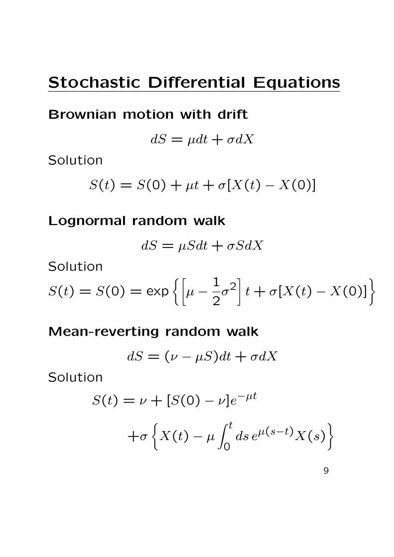
Stochastic Differential Equations

Brownian motion with drift

dS = µdt + σdX

Solution

S(t) = S(0) + µt + σ[X(t)−X(0)]

Lognormal random walk

dS = µSdt + σSdX

Solution

S(t) = S(0) = exp{[

µ−1

2σ2]t + σ[X(t)−X(0)]

}

Mean-reverting random walk

dS = (ν − µS)dt + σdX

Solution

S(t) = ν + [S(0)− ν]e−µt

+σ

{X(t)− µ

∫ t

0ds eµ(s−t)X(s)

}9

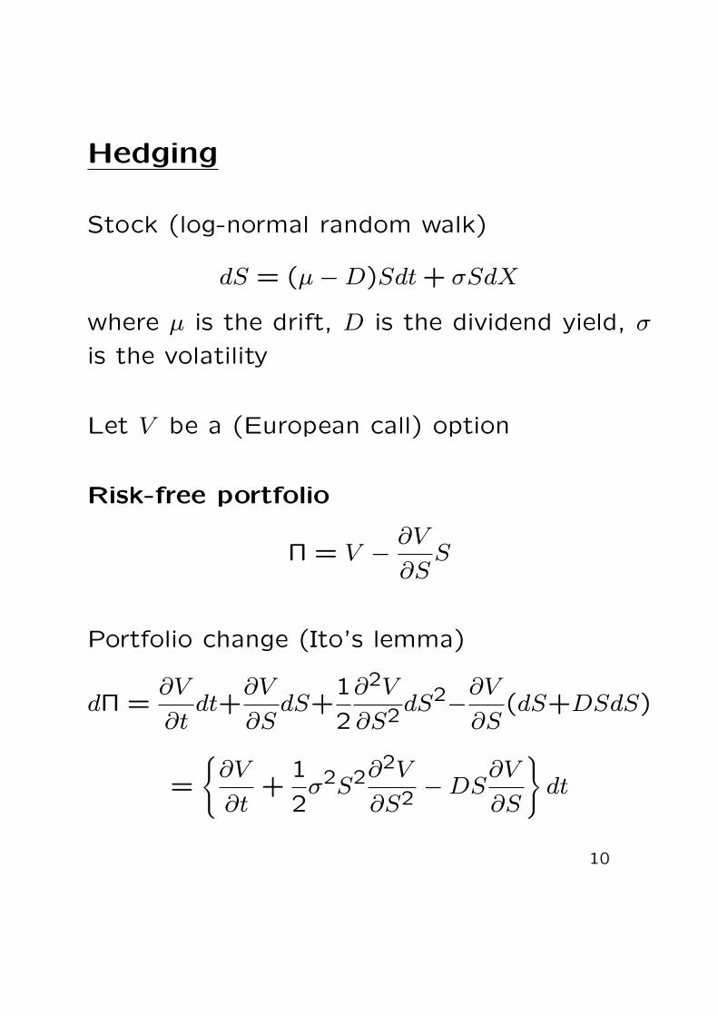
Hedging

Stock (log-normal random walk)

dS = (µ−D)Sdt + σSdX

where µ is the drift, D is the dividend yield, σ

is the volatility

Let V be a (European call) option

Risk-free portfolio

Π = V −∂V

∂SS

Portfolio change (Ito’s lemma)

dΠ =∂V

∂tdt+

∂V

∂SdS+

1

2

∂2V

∂S2dS2−

∂V

∂S(dS+DSdS)

=

{∂V

∂t+

1

2σ2S2∂2V

∂S2−DS

∂V

∂S

}dt

10

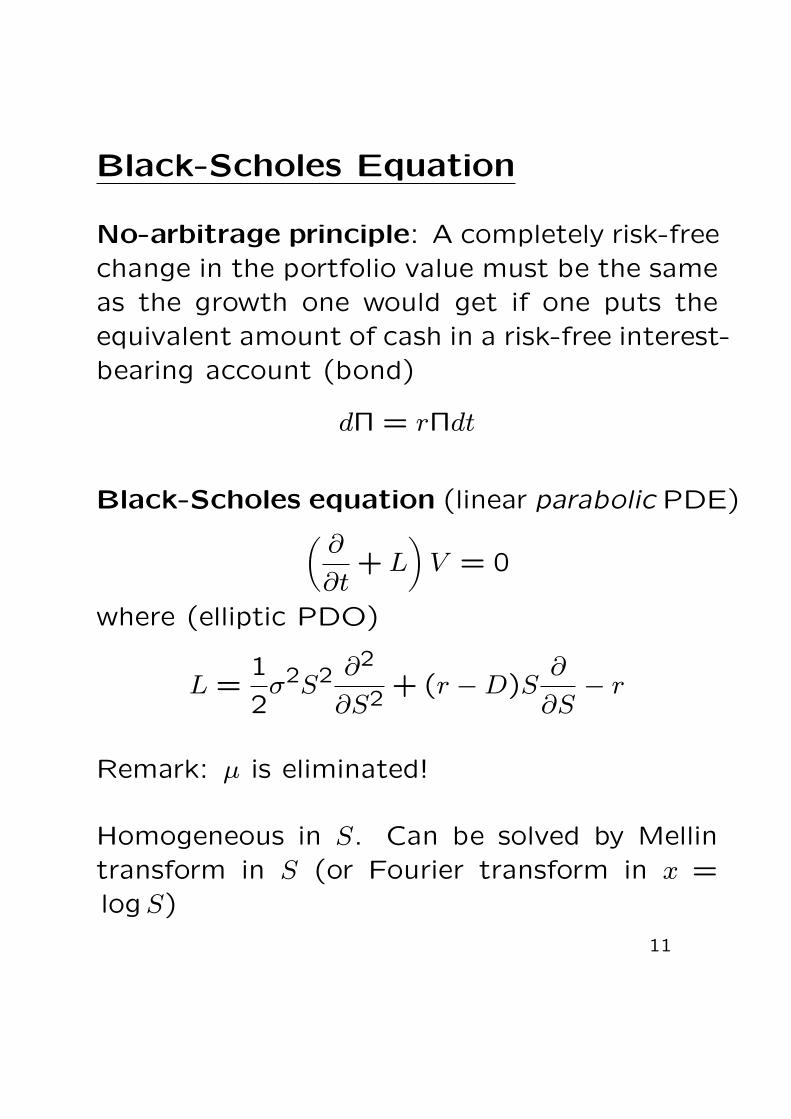
Black-Scholes Equation

No-arbitrage principle: A completely risk-freechange in the portfolio value must be the sameas the growth one would get if one puts theequivalent amount of cash in a risk-free interest-bearing account (bond)

dΠ = rΠdt

Black-Scholes equation (linear parabolic PDE)(∂

∂t+ L

)V = 0

where (elliptic PDO)

L =1

2σ2S2 ∂2

∂S2+ (r −D)S

∂

∂S− r

Remark: µ is eliminated!

Homogeneous in S. Can be solved by Mellintransform in S (or Fourier transform in x =logS)

11

Domain: [0, T ]× R+

Terminal condition

V (T, S) = f(S)

Boundary conditions

V (t,0) = 0 ,

limS→∞

[V (t, S)− S] = 0

12

Payoff Function

f(S) is usually a piecewise linear function

Call : f(S) = (S − E)+

Put : f(S) = (E − S)+

Binary call : f(S) = θ(S − E)

Binary put : f(S) = θ(E − S)

Call spread:

f(S) =1

E2 − E1

[(S − E1)+ − (S − E2)+

]

13

Basket (Rainbow) Options

Multiple assets Si

dSi = (µi −Di)Sidt + σiSidXi

Multiple correlated Winer processes Xi

E(dXi) = 0 E(dXidXj) = ρij

Multi-dimensional Black-Scholes operator

L =1

2

n∑i,j=1

CijSiSj∂2

∂Si∂Sj+

n∑i=1

(r −Di)Si∂

∂Si− r

where

Cij = σiσjρij

Homogeneous in Si. Can be solved by multi-

dimensional Fourier transform in xi = logSi.

14

Assumptions of Black-Scholes

• Hedging is done continuously

• There are no transaction costs

• Volatility is a known constant

• Interest rates and dividends are known con-

stants

• Underlying asset path is continuous

• Underlying asset is unaffected by trade in

the option

• Hedging eliminates all risk

15

Stochastic Volatility

Assume that the volatility of an asset S is afunction of n stochastic factors vi, i = 1,2, . . . , n.

dS = rS dt + σ(t, S, v)S dX

dvi = ai(t, v) dt +n∑

j=1

bij(t, v) dWj

where E(dXdWi) = ρ0i, E(dWidWj) = ρij

Then the valuation operator is

L =1

2σ2S2 ∂2

∂S2+

n∑i=1

AiσS∂2

∂S∂vi

+1

2

n∑i,j=1

Bij ∂2

∂vi∂vj+ rS

∂

∂S+

n∑i=1

ai ∂

∂vi− r

where

Ak(t, v) =n∑

j=1

bkj(t, v)ρj0

Bkl(t, v) =n∑

i,j=1

bki(t, v)ρijbjl(t, v)

16

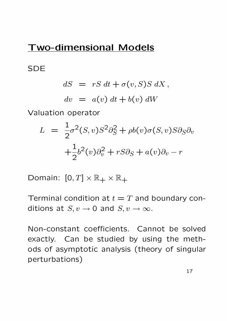
Two-dimensional Models

SDE

dS = rS dt + σ(v, S)S dX ,

dv = a(v) dt + b(v) dW

Valuation operator

L =1

2σ2(S, v)S2∂2

S + ρb(v)σ(S, v)S∂S∂v

+1

2b2(v)∂2

v + rS∂S + a(v)∂v − r

Domain: [0, T ]× R+ × R+

Terminal condition at t = T and boundary con-

ditions at S, v → 0 and S, v →∞.

Non-constant coefficients. Cannot be solved

exactly. Can be studied by using the meth-

ods of asymptotic analysis (theory of singular

perturbations)

17

Jump Process

Poisson process with intensity λ is a stochas-

tic process such that there is a probability λdt

of a jump 1 in Q in the time step dt, that is,

dQ =

0 with probability (1− λdt)

1 with probability λdt

so that,

E(dQ) = λdt

Define the jump process by

dN = −λm dt +(eJ − 1

)dQ

where J is a random variable with the proba-

bility density function ω(J) and

m =

∞∫−∞

dJ ω(J)(eJ − 1

)such that

E(dN) = 0

18

Jump Diffusion with

Stochastic Volatility

SDE

dS = rS dt + σ(v, S)S dX + SdN

dv = a(v) dt + b(v) dW

Assume that there is no correlation between

the Wiener processes X and W and the Poisson

process Q, that is,

E(dXdQ) = E(dWdQ) = 0

19

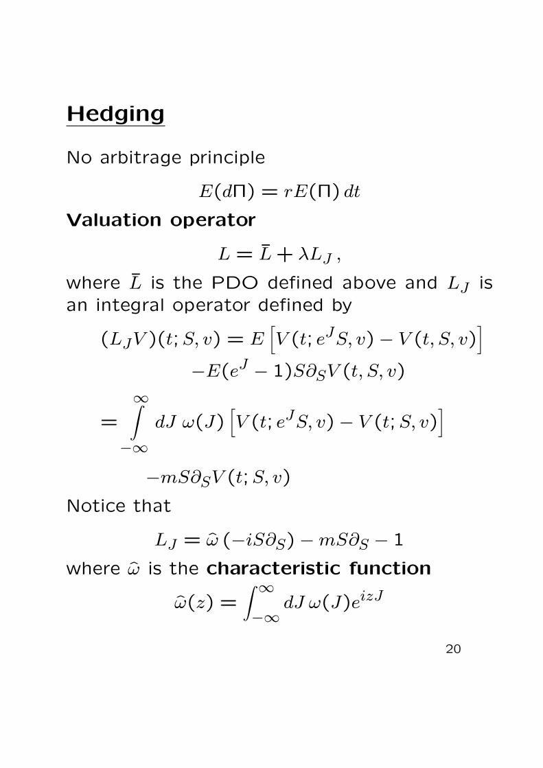
Hedging

No arbitrage principle

E(dΠ) = rE(Π) dt

Valuation operator

L = L̄ + λLJ ,

where L̄ is the PDO defined above and LJ isan integral operator defined by

(LJV )(t;S, v) = E[V (t; eJS, v)− V (t, S, v)

]−E(eJ − 1)S∂SV (t, S, v)

=

∞∫−∞

dJ ω(J)[V (t; eJS, v)− V (t;S, v)

]

−mS∂SV (t;S, v)

Notice that

LJ = ω̂ (−iS∂S)−mS∂S − 1

where ω̂ is the characteristic function

ω̂(z) =∫ ∞−∞

dJ ω(J)eizJ

20

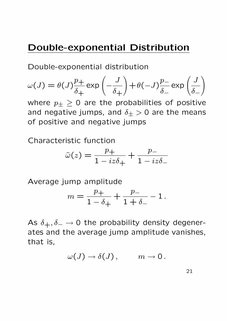
Double-exponential Distribution

Double-exponential distribution

ω(J) = θ(J)p+

δ+exp

(−

J

δ+

)+θ(−J)

p−δ−

exp

(J

δ−

)where p± ≥ 0 are the probabilities of positiveand negative jumps, and δ± > 0 are the meansof positive and negative jumps

Characteristic function

ω̂(z) =p+

1− izδ++

p−1− izδ−

Average jump amplitude

m =p+

1− δ++

p−1 + δ−

− 1 .

As δ+, δ− → 0 the probability density degener-ates and the average jump amplitude vanishes,that is,

ω(J) → δ(J) , m → 0 .

21

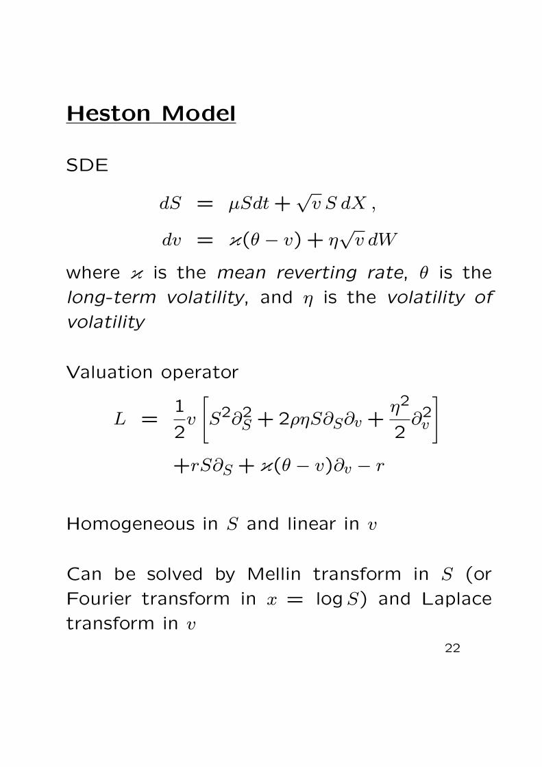
Heston Model

SDE

dS = µSdt +√

v S dX ,

dv = κ(θ − v) + η√

v dW

where κ is the mean reverting rate, θ is the

long-term volatility, and η is the volatility of

volatility

Valuation operator

L =1

2v

[S2∂2

S + 2ρηS∂S∂v +η2

2∂2

v

]

+rS∂S + κ(θ − v)∂v − r

Homogeneous in S and linear in v

Can be solved by Mellin transform in S (or

Fourier transform in x = logS) and Laplace

transform in v

22

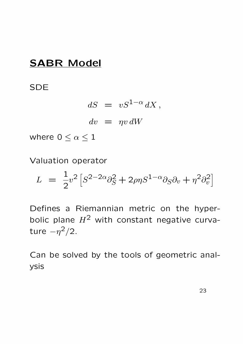
SABR Model

SDE

dS = vS1−α dX ,

dv = ηv dW

where 0 ≤ α ≤ 1

Valuation operator

L =1

2v2[S2−2α∂2

S + 2ρηS1−α∂S∂v + η2∂2v

]

Defines a Riemannian metric on the hyper-

bolic plane H2 with constant negative curva-

ture −η2/2.

Can be solved by the tools of geometric anal-

ysis

23

SABR Model withMean-Reverting Volatility

SDE

dS = vS1−α dX ,

dv = κ(θ − v)dt + ηv dW

Valuation operator

L =1

2v2[S2−2α∂2

S + 2ρηS1−α∂S∂v + η2∂2v

]+κ(θ − v)∂v

Can be solved in perturbation theory in param-

eter κ

24

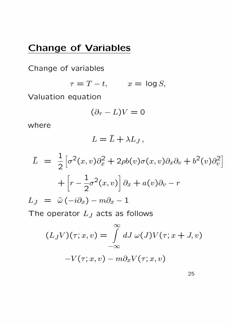
Change of Variables

Change of variables

τ = T − t, x = logS,

Valuation equation

(∂τ − L)V = 0

where

L = L̄ + λLJ ,

L̄ =1

2

[σ2(x, v)∂2

x + 2ρb(v)σ(x, v)∂x∂v + b2(v)∂2v

]+[r −

1

2σ2(x, v)

]∂x + a(v)∂v − r

LJ = ω̂ (−i∂x)−m∂x − 1

The operator LJ acts as follows

(LJV )(τ ;x, v) =

∞∫−∞

dJ ω(J)V (τ ;x + J, v)

−V (τ ;x, v)−m∂xV (τ ;x, v)

25

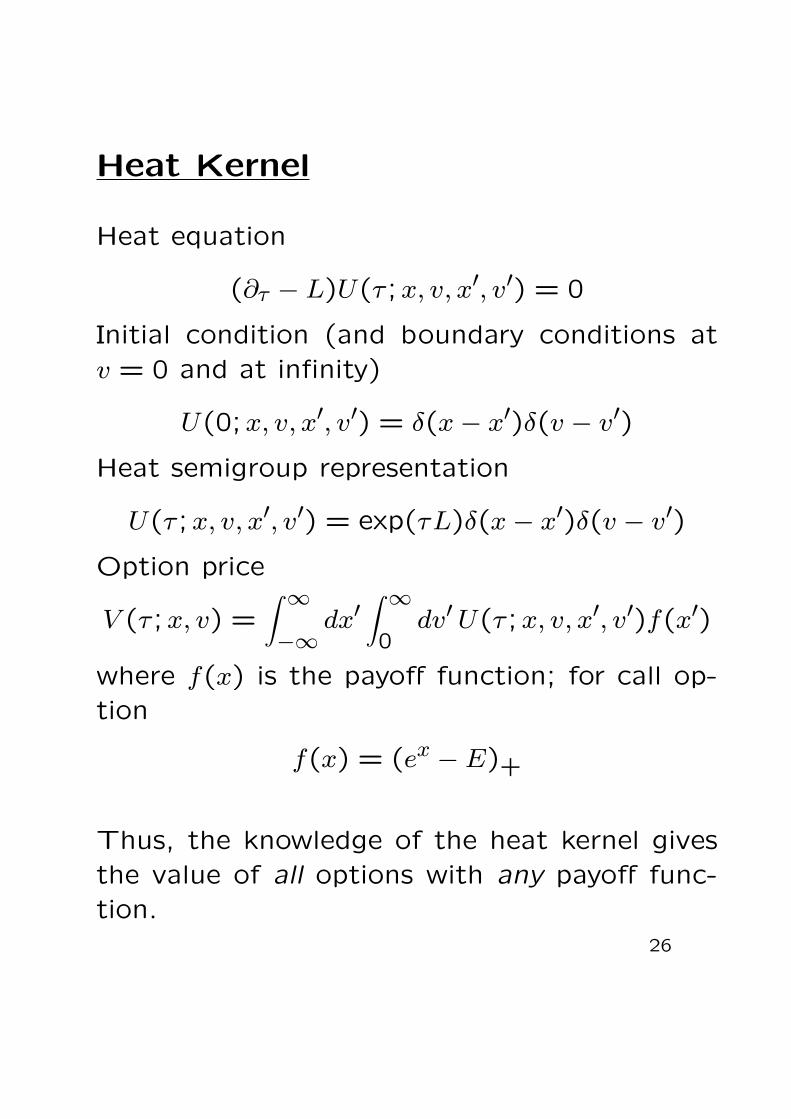
Heat Kernel

Heat equation

(∂τ − L)U(τ ;x, v, x′, v′) = 0

Initial condition (and boundary conditions atv = 0 and at infinity)

U(0;x, v, x′, v′) = δ(x− x′)δ(v − v′)

Heat semigroup representation

U(τ ;x, v, x′, v′) = exp(τL)δ(x− x′)δ(v − v′)

Option price

V (τ ;x, v) =∫ ∞−∞

dx′∫ ∞0

dv′U(τ ;x, v, x′, v′)f(x′)

where f(x) is the payoff function; for call op-tion

f(x) = (ex − E)+

Thus, the knowledge of the heat kernel givesthe value of all options with any payoff func-tion.

26

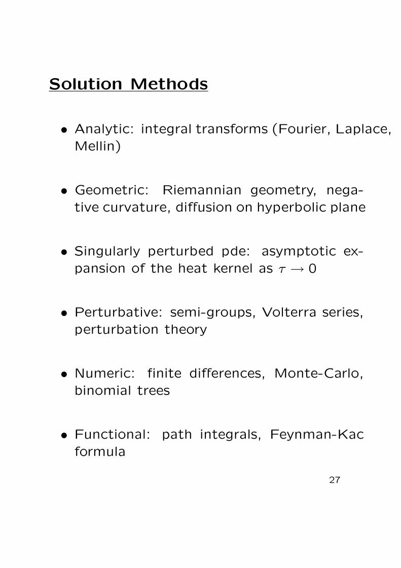
Solution Methods

• Analytic: integral transforms (Fourier, Laplace,Mellin)

• Geometric: Riemannian geometry, nega-tive curvature, diffusion on hyperbolic plane

• Singularly perturbed pde: asymptotic ex-pansion of the heat kernel as τ → 0

• Perturbative: semi-groups, Volterra series,perturbation theory

• Numeric: finite differences, Monte-Carlo,binomial trees

• Functional: path integrals, Feynman-Kacformula

27

Example: Black-Scholes Heat Kernel

Heat Kernel

U(τ ;x, x′) = exp(τL)δ(x− x′)

Valuation operator

L = a∂2x + b∂x − r

where a = σ2

2 , b = r −D − σ2

2

We have

exp(τL) = e−rτ exp (b∂x) exp(a∂2

x

)By using

exp(a∂2

x

)δ(x− x′) = (4πa)−1/2 exp

−(x− x′

)24a

exp (b∂x) f(x) = f(x + b)

we get

U(τ ;x, x′) = (4πa)−1/2 exp

−rτ −(x− x′ + b

)24a

28

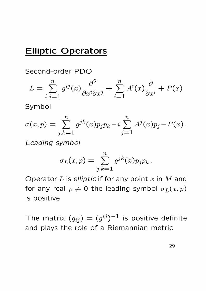
Elliptic Operators

Second-order PDO

L =n∑

i,j=1

gij(x)∂2

∂xi∂xj+

n∑i=1

Ai(x)∂

∂xi+ P (x)

Symbol

σ(x, p) =n∑

j,k=1

gjk(x)pjpk−in∑

j=1

Aj(x)pj−P (x) .

Leading symbol

σL(x, p) =n∑

j,k=1

gjk(x)pjpk .

Operator L is elliptic if for any point x in M and

for any real p 6= 0 the leading symbol σL(x, p)

is positive

The matrix (gij) = (gij)−1 is positive definite

and plays the role of a Riemannian metric

29

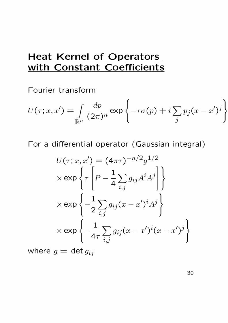
Heat Kernel of Operatorswith Constant Coefficients

Fourier transform

U(τ ;x, x′) =∫

Rn

dp

(2π)nexp

−τσ(p) + i∑j

pj(x− x′)j

For a differential operator (Gaussian integral)

U(τ ;x, x′) = (4πτ)−n/2g1/2

× exp

τ

P −1

4

∑i,j

gijAiAj

× exp

−1

2

∑i,j

gij(x− x′)iAj

× exp

− 1

4τ

∑i,j

gij(x− x′)i(x− x′)j

where g = det gij

30

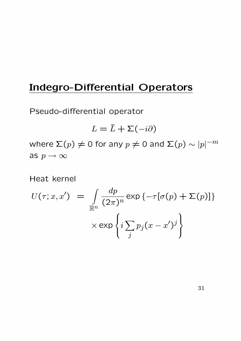
Indegro-Differential Operators

Pseudo-differential operator

L = L̄ + Σ(−i∂)

where Σ(p) 6= 0 for any p 6= 0 and Σ(p) ∼ |p|−m

as p →∞

Heat kernel

U(τ ;x, x′) =∫

Rn

dp

(2π)nexp {−τ [σ(p) + Σ(p)]}

× exp

i∑j

pj(x− x′)j

31

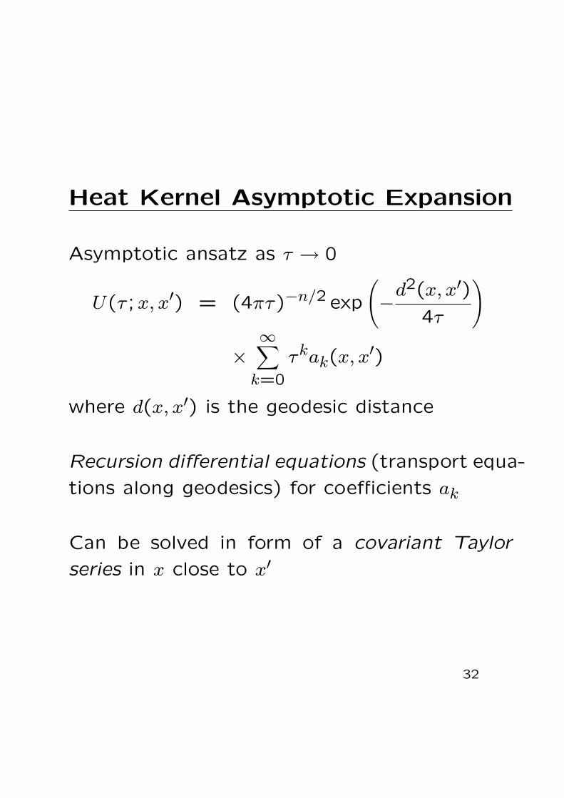
Heat Kernel Asymptotic Expansion

Asymptotic ansatz as τ → 0

U(τ ;x, x′) = (4πτ)−n/2 exp

(−

d2(x, x′)

4τ

)

×∞∑

k=0

τkak(x, x′)

where d(x, x′) is the geodesic distance

Recursion differential equations (transport equa-

tions along geodesics) for coefficients ak

Can be solved in form of a covariant Taylor

series in x close to x′

32

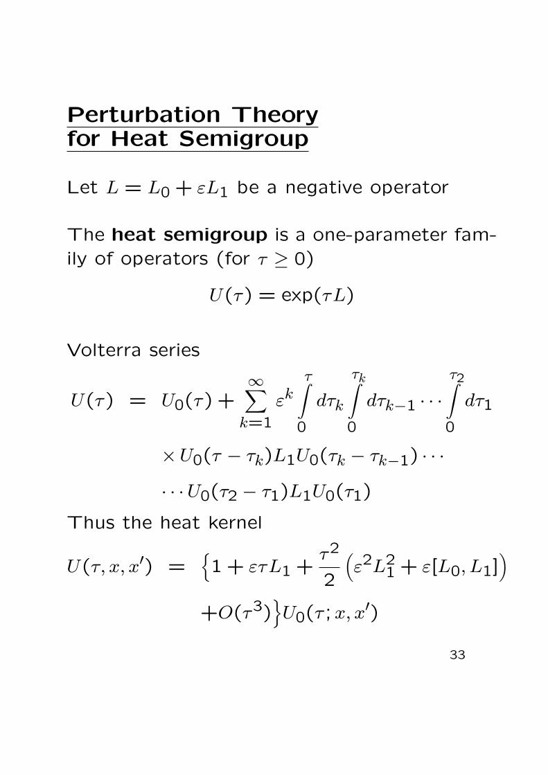
Perturbation Theoryfor Heat Semigroup

Let L = L0 + εL1 be a negative operator

The heat semigroup is a one-parameter fam-ily of operators (for τ ≥ 0)

U(τ) = exp(τL)

Volterra series

U(τ) = U0(τ) +∞∑

k=1

εkτ∫

0

dτk

τk∫0

dτk−1 · · ·τ2∫0

dτ1

×U0(τ − τk)L1U0(τk − τk−1) · · ·

· · ·U0(τ2 − τ1)L1U0(τ1)

Thus the heat kernel

U(τ, x, x′) ={1 + ετL1 +

τ2

2

(ε2L2

1 + ε[L0, L1])

+O(τ3)}U0(τ ;x, x′)

33

Discretization

Let τk = kτ/N , k = 0,1, . . . , N . Then

U(τ) = limN→∞

U(τN − τN−1)U(τN−1 − τN−2)

· · ·U(τ2 − τ1)U(τ1)

Then the heat kernel is

U(τ ;x, x′) = limN→∞

∫RNn

dx1 . . . dxN

U(τN − τN−1, x, xN−1)

×U(τN−1 − τN−2, xN−1, xN−2)

· · ·U(τ2 − τ1, x2, x1)U(τ1, x1, x′)

34

Path Integrals

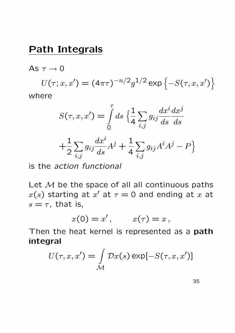
As τ → 0

U(τ ;x, x′) = (4πτ)−n/2g1/2 exp{−S(τ, x, x′)

}where

S(τ, x, x′) =

τ∫0

ds{14

∑i,j

gijdxi

ds

dxj

ds

+1

2

∑i,j

gijdxi

dsAj +

1

4

∑i,j

gijAiAj − P

}is the action functional

Let M be the space of all all continuous pathsx(s) starting at x′ at τ = 0 and ending at x ats = τ , that is,

x(0) = x′ , x(τ) = x ,

Then the heat kernel is represented as a pathintegral

U(τ, x, x′) =∫M

Dx(s) exp[−S(τ, x, x′)]

35