1

TOPICS IN FINANCIAL MARKET RISK

MODELLING

Zishun Ma

A DISSERTATION

in

Quantitative Finance

In partial fulfillment of the Requirements for the Degree of Doctor of Philosophy

25/10/2012

Newcastle Business School

Newcastle University

Newcastle Upon Tyne, UK

2

To my Grandmother

3

Acknowledgement

Studying for a PhD has been a valuable and indispensable experience in my life. When

looking back, I am delighted and at same time grateful for all I have received throughout

these three years. I would like to express my deep and sincere gratitude to my two

supervisors, Prof. Robert Sollis and Dr. Hugh Metcalf, for their generous encouragement and

thoughtful guidance. Prof. Sollis’s and Dr. Metcalf’s wide knowledge and helpful advice

provided a solid basis for this present thesis. Dr. Metcalf’s understanding, encouragement and

personal guidance have been invaluable to me on both an academic and a personal level.

Without their support, this thesis would not have been possible. I am also deeply indebted to

my colleagues and friends in the Newcastle Business School that have provided the

environment for sharing their experiences and thoughts with me. I would especially like to

thank my two colleagues and best friends, Hangxiong Zhang and Fengyuan Shi, for their

extremely valuable support and insights in my PhD study.

I own my loving thanks to my parents, Lilin Wang and Chenggang Ma, and my beloved

girlfriend, Yongying Yu. Their selfless love and care have provided me inspiration and

power. Without their encouragement and understanding it would have been impossible for

me to finish this work. I owe them everything and here I just wish to show them how much I

love and appreciate them.

Finally I would like to thank all of people and friends whom I know for their help.

4

DECLARATION OF AUTHENTICITY

This thesis contains no material which has been accepted for the award of any other degree or

diploma in any University, and is less than 100,000 words in length. To the best of my

knowledge and belief, this thesis contains no material previously published or written by

another person, except where due reference has been made.

5

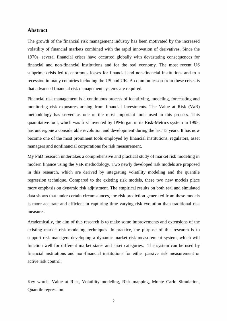
Abstract

The growth of the financial risk management industry has been motivated by the increased

volatility of financial markets combined with the rapid innovation of derivatives. Since the

1970s, several financial crises have occurred globally with devastating consequences for

financial and non-financial institutions and for the real economy. The most recent US

subprime crisis led to enormous losses for financial and non-financial institutions and to a

recession in many countries including the US and UK. A common lesson from these crises is

that advanced financial risk management systems are required.

Financial risk management is a continuous process of identifying, modeling, forecasting and

monitoring risk exposures arising from financial investments. The Value at Risk (VaR)

methodology has served as one of the most important tools used in this process. This

quantitative tool, which was first invented by JPMorgan in its Risk-Metrics system in 1995,

has undergone a considerable revolution and development during the last 15 years. It has now

become one of the most prominent tools employed by financial institutions, regulators, asset

managers and nonfinancial corporations for risk measurement.

My PhD research undertakes a comprehensive and practical study of market risk modeling in

modern finance using the VaR methodology. Two newly developed risk models are proposed

in this research, which are derived by integrating volatility modeling and the quantile

regression technique. Compared to the existing risk models, these two new models place

more emphasis on dynamic risk adjustment. The empirical results on both real and simulated

data shows that under certain circumstances, the risk prediction generated from these models

is more accurate and efficient in capturing time varying risk evolution than traditional risk

measures.

Academically, the aim of this research is to make some improvements and extensions of the

existing market risk modeling techniques. In practice, the purpose of this research is to

support risk managers developing a dynamic market risk measurement system, which will

function well for different market states and asset categories. The system can be used by

financial institutions and non-financial institutions for either passive risk measurement or

active risk control.

Key words: Value at Risk, Volatility modeling, Risk mapping, Monte Carlo Simulation,

Quantile regression

6

Table of Contents

Table of figures .......................................................................................................................... 9

1 Introduction ........................................................................................................................... 11

1.1 The need for the financial risk management .................................................................. 11

1.2 General introduction of Value at Risk in the financial risk management ...................... 13

1.3 Research contributions of the thesis ............................................................................... 14

1.4 Structure of the thesis ..................................................................................................... 18

2 Literature review of the financial market risk modeling ...................................................... 20

2.1 Building blocks of Value at Risk models ....................................................................... 20

2.1.1 Non-parametric VaR model ..................................................................................... 21

2.1.2 Parametric VaR model ............................................................................................. 22

2.1.3 Semi-parametric VaR model and Extreme Value Theory ....................................... 24

2.1.4 CAViaR model ......................................................................................................... 26

2.2 Combining risk exposure modeling with VaR models ................................................... 28

2.2.1 Local-valuation approach ......................................................................................... 29

2.2.2 Full-valuation approach............................................................................................ 31

2.3 Risk decomposing by VaR models ................................................................................. 34

2.3.1 Marginal VaR ........................................................................................................... 34

2.3.2 Incremental VaR and best hedge ratio ..................................................................... 35

2.4 Risk integration techniques ............................................................................................ 36

2.4.1 Regression analysis .................................................................................................. 37

2.4.2 Principle Component Analysis ................................................................................. 38

2.5 Risk overlay on multi-time horizon ................................................................................ 39

2.5.1 Factors considered in the VaR models ..................................................................... 40

2.5.2 Multi-day VaR from IGARCH model ..................................................................... 40

2.5.3 Multi-day VaR from ARMA-GARCH model ......................................................... 42

2.5.4 An ideal of accuracy improvement .......................................................................... 44

2.6 Conclusion ...................................................................................................................... 45

3 Application of VaR models in the financial market risk measurement ................................ 47

3.1 Dataset ............................................................................................................................ 47

3.2 Risk measurement of the equity portfolio ...................................................................... 48

3.2.1 Equity risk assessment ............................................................................................. 49

3.2.2 Risk integration of the equity portfolio .................................................................... 51

3.2.3 Time varying conditional distribution on VaR estimates ........................................ 54

7

3.3 Risk measurement of the future and option portfolio ..................................................... 58

3.3.1 Empirical results from Local valuation approach .................................................... 59

3.3.2 Empirical results from Full valuation approach ....................................................... 63

3.4 Risk measurement of the foreign currency ..................................................................... 66

3.4.1 Findings from the local valuation approach ............................................................. 66

3.4.2 Empirical analysis .................................................................................................... 68

3.5 Risk measurement of the bond portfolio ........................................................................ 72

3.5.1 Risk profile analysis in the UK bond market ........................................................... 72

3.5.2 Risk measurement integrating the mapping techniques ........................................... 79

3.6 Summary of the empirical findings from the model application .................................... 85

3.7 Back-testing the model performance .............................................................................. 87

3.7.1Brief review of the back-testing models ................................................................... 87

3.7.2 Application of the back-testing models .................................................................... 89

3.7.3 Empirical results summary ....................................................................................... 95

4. Two Step Dynamic Adjusted VaR model ............................................................................ 97

4.1 Introduction .................................................................................................................... 97

4.2 Brief review of the Dynamic adjustment approach ........................................................ 98

4.2.1 Dynamic VaR on the time-varying volatility ........................................................... 99

4.2.2 Dynamic VaR on time-varying quantile ................................................................ 100

4.3 Two-Step Dynamic Adjusted VaR model .................................................................... 101

4.4 Data and empirical results ............................................................................................ 105

4.4.1 Empirical results from the historical data .............................................................. 105

4.4.3 Empirical results from the simulated data .............................................................. 117

4.4.4 Multiday VaR generation from TSDA-VaR model ............................................... 126

4.5 Conclusion .................................................................................................................... 127

5. Generating volatility forecasts from ARMAX process ..................................................... 129

5.1 Introduction .................................................................................................................. 129

5.2 Literature review of the volatility models .................................................................... 131

5.2.1 Time series volatility model ................................................................................... 131

5.2.2 Stochastic volatility model ..................................................................................... 133

5.2.3 Extracting volatility from symmetric quantile interval .......................................... 134

5.3 Volatility modeling using ARMAX process ................................................................ 134

5.4 Data and empirical results ............................................................................................ 138

8

5.4.1 Estimate the symmetric quantile ............................................................................ 138

5.4.2 ARMAX modeling on the dynamic symmetric quantile intervals ......................... 144

5.4.3 Empirical comparison of the different volatility forecast approaches ................... 148

5.5 Some extensions ........................................................................................................... 154

5.5.1 ARMAX process for volatility forecasts ................................................ 154

5.5.2 A comparison between ARMAX process and Taylor’s approach ......................... 158

5.6 Conclusion .................................................................................................................... 161

6. Final Remarks .................................................................................................................... 163

7. References ………………………………………………………………………………. 163

9

Table of figures

Figure 1: The historical price series of S&P 500 index from 2001 to 2010 ......................................................... 48

Figure 2: Histogram, normal distribution and EVT tail distribution of the first corner portfolio using 2 year

historical prices from 16/08/2007 to 25/06/2009 .................................................................................................. 50

Figure 3: Best Hedge amount of the individual stocks in the portfolio (By decomposing the parametric VaR in

the table 3) ............................................................................................................................................................ 53

Figure 4: The daily historical price series of FTSE 100 index from 2001 to 2010 ............................................... 55

Figure 5: Conditional volatility series of FTSE 100 index extracted from the treed selected GARCH models

(Blue line: EGARCH. Green line:GJR-GARCH. Black line:GARCH ) .............................................................. 56

Figure 6: Conditional VaR forecast series of FTSE100 from 07/05/2009 to 31/07/2010..................................... 56

Figure 7: Implied volatility of FTSE100 European options from 26/06/2009 to 11/06/2010 ............................... 59

Figure 8: Historical prices of FTSE 100 min-future contracts from 26/06/2009 to 11/06/2010 ........................... 60

Figure 9: The Monte Carlo simulation with 250 paths and over 15 days (Input data: FTSE 100 index price from

14/06/2008 to 14/06/2010) ................................................................................................................................... 64

Figure 10: The density plot of the simulated prices on 15/03/2010 ...................................................................... 65

Figure 11: Historical prices of Foreign currency forward contracts from 2009 to 2011(sterling against US dollar)

.............................................................................................................................................................................. 69

Figure 12: One year zero rate curve in the UK and the US market from 2009 to 2010 ........................................ 70

Figure 13: The historical return series of UK Treasury Coupon Strips (from 2006 to 2011) ............................... 74

Figure 14: The UK zero rate yield surface maturity from 1 year to 30 years (Sample period spanning from 2006

to 2011) ................................................................................................................................................................. 76

Figure 15: Historical price of S&P 500 index (From 13/08/2007 to 11/08/2009) ................................................ 90

Figure 16: VaR estimate at 95% confidence level (Input data: historical prices of S&P 500 index from

24/08/2008 to 24/06/2009) ................................................................................................................................... 91

Figure 17: VaR estimates on the two simulated series (Top: GARCH simulation, Bottom: sample variance

simulation) ............................................................................................................................................................ 93

Figure 18: Daily VaR estimates of the FTSE 100 index return from 2002 to 2009 ............................................. 94

Figure 19: 10-day VaR forecast series of FTSE 100 index from 2002 to 2009 .................................................... 95

Figure 20: Historical prices of FTSE 100 index from 18/10/2001 to 15/10/2010. (a)Index daily prices (b) Index

daily returns (c) QQ plot of the returns (d) Kernel density of the returns........................................................... 105

Figure 21: Sample return ACF and Squared return PACF of FTSE 100 returns from 18/10/2001 to 15/10/2010

............................................................................................................................................................................ 106

Figure 22: AIC and BIC Information Criterion for the nine selected GARCH models ...................................... 107

Figure 23: Forecasted daily VaR series of FTSE 100 returns from 11/10/2002 to 28/12/2010 .......................... 107

Figure 24: Estimated daily Expected Shortfall of FTSE 100 index from 11/10/2002 to 15/08/2009 ................. 110

Figure 25: Dynamic daily VaR series from there VaR models. Red line: VaR from Adaptive-CViaR. Green line:

VaR from TSDA-VaR. Blue line: VaR from Asymmetric Slope-CAViaR ........................................................ 113

Figure 26: The sample paths of the simulated prices (with 1877 observations) ................................................. 120

Figure 27: The Symmetric quantile forecast from 1911/2004 to 16/11/2010 (quantile Level p = 2.5%) ........... 140

Figure 28: The Dynamic symmetric quantile Intervals at quantile level p= 5% ................................................. 143

Figure 29: Daily volatility forecasts of FTSE 100 index from ARMAX process, spanning from 22/10/2002 to

11/08/2010 .......................................................................................................................................................... 146

Figure 30: Plot of the Standardized Returns from the ARMAX process ............................................................ 147

Figure 31: Density comparison of the original and the Standardized Returns .................................................... 147

Figure 32: ACF and PACF of the Standardized Returns .................................................................................... 148

Figure 33: Comparison between three volatility forecast series. Red line: ARMAX volatility. Green line:

EWMA volatility. Purple line: TGARCH volatility ........................................................................................... 150

Figure 34: Daily Volatility FORECAST FROM the ARMAX model and the LS regression by Taylor ........... 159

10

Table 1: Risk and return of five corner portfolios in the efficient frontier (Based on the 2 year historical PRICES

from 16/08/2007 to 25/06/2009) ........................................................................................................................... 49

Table 2: Comparison results of three SELECTED VAR approaches ON 26/06/2009 ......................................... 50

Table 3: The portfolio VaR estimates using PCA and diagonal model on 26/06/2009 (at 5% VaR confidence

level) ..................................................................................................................................................................... 52

Table 4: Back-testing results (Compare VaR series with FTSE100 actual returns FROM 07/05/2009 to

31/07/2010) ........................................................................................................................................................... 57

Table 5: The DELTA and GAMMA exposure of the targeting portfolio on 11/01/2010 (The portfolio consists of

20,000 FTSE 100 european put options and 20,000 FTSE 100 future contract maturated on 18/06/2010) ......... 60

Table 6: The total realized loss of the targeting portfolio on 12/01/2010 ............................................................. 61

Table 7: Market price of FTSE 100 European OPTIONS ON 09/03/10 .............................................................. 62

Table 8: EWMA-Covariance matrix of the foreign currency estimated on 20/12/2012 (sterling against US dollar)

.............................................................................................................................................................................. 71

Table 9: Risk decompose of 1 year foreign currency contract (sterling against US dollar) on 20/12/2010 ......... 71

Table 10: Historical prices of UK treasury coupon strip on 07/12/2010 (Maturity from 1 year to 30 years) ....... 73

Table 11: UK Treasury Coupon Strips VaR estimate using duration model on 07/12/2010 (Input data: Historical

prices from 10/11/2006 to 06/12/2010) ................................................................................................................ 75

Table 12: The correlation matrix of the UK zero yields (Estimated using sample data from 2006 to 2011) ....... 76

Table 13: PCA results of the UK zero rates matrix from table 12 ........................................................................ 77

Table 14: The covariance matrix constructed by full sample returns from 2006 to 2011..................................... 78

Table 15: The covariance matrix constructed by PCA ......................................................................................... 79

Table 16: The bond portfolio VaR estimate on 07/12/2010 using duration and PCA .......................................... 81

Table 17: The realized loss of the bond portfolio on 21/12/2010 ......................................................................... 82

Table 18: The selected UK corporate bonds information on 07/12/2010 ............................................................. 84

Table 19: The future cash flows of the targeting bond portfolio (Consists of £100m investment in each corporate

bond shown in the table 18) .................................................................................................................................. 84

Table 20: EWMA covariance MATRIX OF 5 year and 6 year UK zero bond (Based on the sample period from

2009 to 2010) ........................................................................................................................................................ 84

Table 21: The bond Portfolio VaR estimate on 07/12/2010 using vertex mapping .............................................. 85

Table 22: Back-testing result (compare the VaR estimates with the actual S&P 500 index returns FROM

24/08/2008 to 24/06/2009) ................................................................................................................................... 91

Table 23: Back-testing result for conditional VaR forecast FROM 11/10/2002 to 15/08/2009 ......................... 108

Table 24: QUANTILE REGRESSION result using window data from 11/10/02 to 11/10/06 ( ) ......... 111

Table 25: QUANTILE REGRESSION result using window data from 11/10/02 to 11/10/06 ( ) ....... 111

Table 26: Back-testing result of dynamic VaR forecast FROM 11/12/02 to 15/08/2009 ................................... 114

Table 27: Efficiency test result of dynamic VaR forecast FROM 11/12/02 to 15/08/2009 ................................ 116

Table 28: The setting of input values in the three simulation process ................................................................ 119

Table 29: Quantile Estimation result for the three VaR models FROM the SIMULATED PRICE ................... 122

Table 30: Back-testing result from simulateld data ............................................................................................ 124

Table 31: Efficiency test from simulateld data (99% VaR confidence level) ..................................................... 125

Table 32: Efficiency test from simulateld data (95% VaR confidence level) ..................................................... 126

Table 33: Estimation result of the quantile regression model (Input data: FTSE 100 index price from 19/11/2001

to 16/11/204) ...................................................................................................................................................... 140

Table 34: Back-testing result of the symmetric quantile estimate at selected three quantile level ..................... 143

Table 35: Parameter Estimation of ARMAX model under three selected sample periods ................................. 145

Table 36: Parameter Estimation of TGARCH (1,1) Model over three selected sample periods ........................ 149

Table 37: Correlation Coefficient and mean absolute error between the actual returns and the estimated volatility

............................................................................................................................................................................ 152

Table 38: Results of the Encompassing test for the three volatility series .......................................................... 154

Table 39: Parameter estimation of General ARMAX process ( Two Sub-sample periods) ............................... 157

Table 40: Parameter estimation of General ARMAX process (Whole-sample period) ...................................... 158

Table 41: Encompassing test between the ARMAX volatility and the volatility from Taylor’s regression ....... 161

11

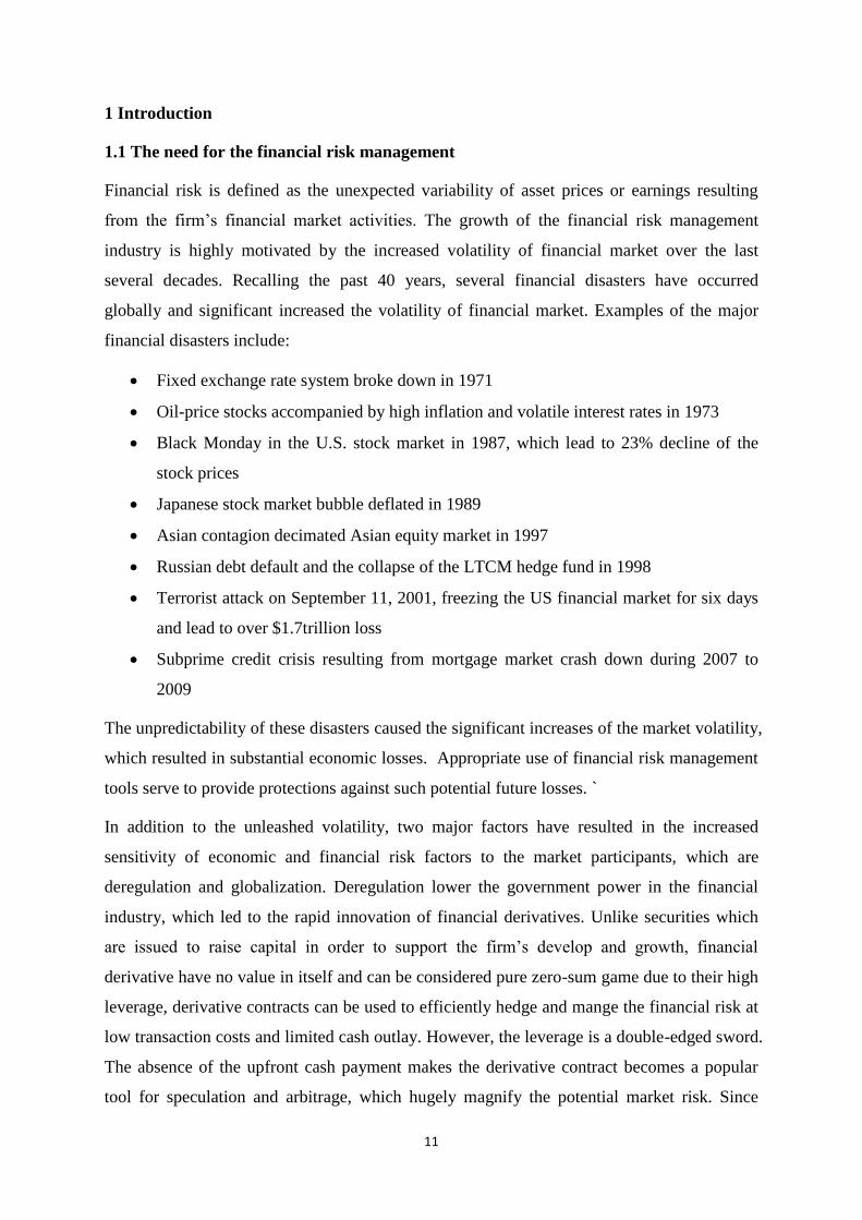
1 Introduction

1.1 The need for the financial risk management

Financial risk is defined as the unexpected variability of asset prices or earnings resulting

from the firm’s financial market activities. The growth of the financial risk management

industry is highly motivated by the increased volatility of financial market over the last

several decades. Recalling the past 40 years, several financial disasters have occurred

globally and significant increased the volatility of financial market. Examples of the major

financial disasters include:

Fixed exchange rate system broke down in 1971

Oil-price stocks accompanied by high inflation and volatile interest rates in 1973

Black Monday in the U.S. stock market in 1987, which lead to 23% decline of the

stock prices

Japanese stock market bubble deflated in 1989

Asian contagion decimated Asian equity market in 1997

Russian debt default and the collapse of the LTCM hedge fund in 1998

Terrorist attack on September 11, 2001, freezing the US financial market for six days

and lead to over $1.7trillion loss

Subprime credit crisis resulting from mortgage market crash down during 2007 to

2009

The unpredictability of these disasters caused the significant increases of the market volatility,

which resulted in substantial economic losses. Appropriate use of financial risk management

tools serve to provide protections against such potential future losses. `

In addition to the unleashed volatility, two major factors have resulted in the increased

sensitivity of economic and financial risk factors to the market participants, which are

deregulation and globalization. Deregulation lower the government power in the financial

industry, which led to the rapid innovation of financial derivatives. Unlike securities which

are issued to raise capital in order to support the firm’s develop and growth, financial

derivative have no value in itself and can be considered pure zero-sum game due to their high

leverage, derivative contracts can be used to efficiently hedge and mange the financial risk at

low transaction costs and limited cash outlay. However, the leverage is a double-edged sword.

The absence of the upfront cash payment makes the derivative contract becomes a popular

tool for speculation and arbitrage, which hugely magnify the potential market risk. Since

12

1986, the derivatives markets have grown from $1,083 billion to $ 343 trillion in 20051.

Along with this growth, many financial entities suffered huge losses involving the derivatives.

Capital Market Risk Advisor, a consulting firm, has estimated that the speculative losses

attributed to derivatives amounted to over $30 billion during the 1990s. The collapse of

Barings bank in the UK financial market is a typical example of misusing the derivatives for

speculation.

Globalization, on the other hand, lowers the barriers to global trade and investment, which

leads to the firms undertaking more international business and thereby causes them exposing

more risk in the international financial market. These changes have also significantly

increased the financial market risk, thereby raising the need and importance of the financial

risk management.

The goal of the financial risk management is not to minimize or eliminate risk, but to bring

the economic value to the entity who utilizes it. From the perspective of corporations,

appropriate use of the financial risk management tools helps them to reduce the potential

costs of financial distress and bankruptcy. To be specific, when a firm has debt in its capital

structure, the increased risk of its asset will increase the probability that the firm will unable

to repay the liability to its debt holders and thereby increase the bankruptcy cost. Even if the

bankruptcy can be avoided, the firm with high risky equity will experience the cost so called

financial distress, which includes the lost sales from the counterparties or the difficulty of

refinancing in the market. The idiosyncratic risk generated from the bankruptcy and financial

distress cannot be hedged by the individual shareholder as beta risk and could only be

appropriate managed if the firm owns a good risk management system.

The financial risk management system is even more critical to the financial institutions. One

primary function of the financial institutions is to serve as the intermediaries for managing

the financial risk. For instance, they create markets and instruments to share and hedge the

financial risk faced by the firms, provide risk advisory services and act as counterparty for the

risk transfer. It is exactly these roles that force the financial institutions to understand and

price the risk properly. A well-functioned risk management system will help financial

institutions to measure the financial risk as precisely as possible and thereby help them to be

better prepared for the adverse consequence from such risk.

1 Source: Bank of International Settlements 2005

13

Furthermore, regulators require a mature and effective financial risk management system to

help them to maintain the health and stability of the entire financial markets. The need of

regulations for the financial risk control is originally due to the existence of the moral hazard.

Given the fact that financial institutions gather funds from investors and invest the investors’

funds for return enhancement, there will be less incentive for the owners of the financial

institutions to control the risk properly. Because if they take risks and prosper, they will

partake in the benefits and if they lose, the investors suffer the direct consequences of the loss.

Similarly, for the non-financial institutions, there exists the information asymmetry between

the management and the shareholders. If the compensation of the management is highly

depends the investment performance, the manger will be more insensitive to take high risky

project, which will adversely affect the interests of the shareholders.

The existence of the moral-hazard problem explains why the regulators need the risk

management system to control the risk-taking activities. If the firms and the financial

institutions are allowed to freely decide on their own economic risk capital, the traders and

the managers will implement increasingly risky activities, which increase the probability of

bankruptcy. Furthermore, the effect of externalities might rise when one institution’s failure

affects other firms, which eventually pose a threat to the stability of the entire financial

system.

1.2 General introduction of Value at Risk in the financial risk management

Financial risk management is a continuous process of identifying, modeling, forecasting and

monitoring the risk exposures raised from the financial market activities. One of the major

tools used to model the financial risk is Value at Risk. This methodology, which was first

invented by J.P. Morgan in its Risk-Metrics system in 1995, has rapidly becomes the most

prominent applied risk measurement tool in the financial field over the last several decades.

Simply speaking, VaR is defined as the maximum potential loss of the corresponding

financial portfolio’ market value at given confidence level and over fixed time horizon.

Assume a risk manager estimate the daily VaR at 5% confidence level as £10,000, this value

indicates that there is a 95% chance that the next day loss of his portfolio’ market value will

not exceed £10,000. In other words, there is only 5% chance that the portfolio will experience

a loss of £10,000 or more.

Statistically, given confidence level, VaR is the quantile of the portfolio value’s

probability distribution, which is expressed as:

14

(1.1)

where is the inverse function of the portfolio’s cumulative distribution

Artzner and Delbaen (1999) further developed C-VaR (Tail Conditional VaR) as a

complement of the standard VaR measure, which takes into account the magnitude of the loss

over the VaR estimate. This measurement is interpreted as the expected size of the loss

condition on the loss has exceeded the VaR estimate, which is expressed as:

(1.2)

The most appealing feature of VaR measure is that it summarizes the overall market risk

components into a single numerical value. Besides, it is an ex-ante measure which means that

it could be applied by the risk managers for a forward-looking risk control. Due to these

properties, VaR has spread well over the last several decades in the financial industry and by

now it has becomes the benchmark measurement of the financial market risk for both

institutions and regulators. The application of VaR methods can be classified as follows:

Passive risk reporting: The banks and institutions that deal with large-scaled

portfolios and complicated instruments are applied VaR to apprise the market risk run

by the trading and investment operations. U.S. Securities and Exchange Commission

ruled the public corporations to disclose their quantitative financial risk exposure

using VaR in 1997.

Defensive risk controlling: VaR are now commonly used by the financial institutions

to set position limits for the traders and business units. The minimum capital

requirement set by Basel Committee 2is directly based on VaR methods

Active risk management: The Risk-Adjust Performance Measures (RAPMs) based on

VaR such as RAROC is now used increasingly by the financial and non-financial

institutions to allocation appropriate capital across the traders, business units and even

the whole institutions. VaR could also assists the portfolio managers to create greater

Shareholder Value Added (SVA)

1.3 Research contributions of the thesis

Following by the existing VaR methods, my PhD research undertakes a comprehensive and

practical study of the market risk modeling techniques in the modern finance. Generally

speaking, the main contribution of this research lies in two areas, which are model application

2 See Basel Accord 1988, Basel Accord 2004

15

and model innovation. The model application is attempting to formulate some applicable

rules of how to select appropriate risk models under the different market conditions and

different asset categories. Particularly, we proposed several selection criterions of the VaR

models based on our empirical analysis. These criterions include:

Firstly, the choice of the appropriate VaR model should highly depends on the risk degree of

the target portfolio, rather than the overall market condition. Our empirical results shows that

as the hypothetical portfolio become more risky (as we move alongside the efficient frontier),

the parametric VaR model becomes less reliable than the semi-parametric VaR model. The

implication of this criterion is that even the market is at the high volatility regime, the risk

managers could still apply the parametric VaR model as long as the target portfolio is at

moderate risk level. However, if the risk managers are facing the high risky portfolio in

practice, the semi-parametric VaR on EVT is preferable for a more conservative risk

measurement.

Secondly, the VaR estimate generated from GARCH volatility should be a safe risk

measurement model, as long as the GARCH estimation is dynamically updated on daily basis.

We explain this statement from two aspects: On one hand, the risk managers should be less

worried about the underestimation problem from the VaR when the current market is at high

volatility regime3, because our empirical results shows that under such circumstance the

GARCH types of models could generate a even higher volatility forecast than those from the

market expectation (implied volatility). On the other hand, if the current market is at normal

condition, the GARCH types of model might generate a lower volatility forecast than that

from the Implied Volatility. However, the VaR estimate should still be safe, since the

quantile multiplier which captured the extreme risk at normal market condition could serve as

a complement.

Thirdly, if the time varying distribution has already been considered by the GARCH volatility,

the choice of the quantile estimator will have limited effect on the VaR estimate at low

confidence level. In the other word, the underestimate problem from the standard normal

quantile compared to the EVT will tend to disappear at lower VaR confidence level (say

95%), provided that the dynamicity has been adjusted by the GARCH volatility. However,

this conclusion may not be comprehensive since we have not verified this statement through

different sets of financial data. But it at least indicate that the time varying quantile could be

3 This research define the high volatility regime if the daily unconditional Volatility above 2%, according to the

research by Tsay (2003)

16

possibly captured by the GARCH volatility in the VaR modeling, which provide a useful

implication for the dynamic improvement of the risk models. The dynamic CAViaR model

proposed in the chapter 4 is highly motivated by this result.

Fourthly, the selection of the risk exposure modeling technique should depend on the

monotonicity of the target portfolio. Our empirical result from the hypothetic portfolios

shows that when the payoff of the target portfolios is monotonic, the local valuation model

will perform well, with enough speed and accuracy. On the other hand, this model seriously

underestimates the market risk when the target portfolio has non-monotonic payoff. The full

valuation model, however, could provide a reasonable risk assessment under such situation.

The approach is theoretically more accurate than the local valuation model due to its more

comprehensive risk consideration. However, its accuracy is highly depends on the

appropriate selection of the particular stochastic process for the underlying risk factors.

Besides, the approach is fairly time intensive to implement which needs substantial

computational time.

Fifthly, our empirical analysis of the foreign currency forward shows that although the

exchange rate risk is the main concern when measuring the foreign currency risk, the interest

rate risk need be considered additionally as time elapsed from the initial evaluation date.

Since when time moves away from the initial evaluation date, the interest rate risk cannot be

fully hedged by the unequaled long-short position in the zero bonds.

Finally, the empirical results from the UK bond market indicated that PCA outperform the

duration model in both bond risk profile analysis and bond risk measurement. Historical term

structure of the UK zero yields indicates that the yield curve undergone a certain degree of

unparallel shift. When the bond portfolio is dominated by the long-short strategy of different

maturity bonds, the unparallel shift movement becomes the core risk factor rather other the

parallel shift measured by the duration model, which leading to the underestimation problem

from the VaR estimate adopted by the duration model. Furthermore, the time decay effect in

the price series will be completely overlooked in the duration model. This flaw could lead to

a mislead correlation generated from the duration model, which in fact is due to the synthetic

time decay effect from the historical bond prices.

These empirical findings from the model application provide us some useful implications for

the model improvement and thereby contribute to further model innovation in my PhD study.

To be specific, we propose two newly developed risk models in the latter stage of our

17

research. Motivated by the idea of integrating the effect of GARCH volatility and time

varying quantile into VaR modeling, we proposed a Two-Step Dynamic Adjusted risk model

in chapter four. This model has several innovation points. Firstly, given that the

autoregressive term of the VaR estimates are re-estimated by the GARCH volatility at daily

frequency, both time varying volatility and time varying quantile have been taken into

account by this model. Secondly, the estimated VaR series on GARCH volatility should

encompass certain effect of the nonlinear evolution of the Quantile, which is ignored in the

linear specification of the traditional CAViaR model. Thirdly, a time varying smoothing

factor is introduced in this CAViaR model. This amendment is aim to alleviate the limitation

generated from the Engel’s Adaptive CAViaR, in which the VaR prediction will increase by

the same amount regardless of whether the returns exceed the previous VaR estimate by

small or by large amount. Finally, the selected exogenous variable in this model will allow us

to find out other possible factor that have relationship with the time varying risk evolution

and hence further improve the forecast accuracy. The back-testing results based on both real

and simulated data shows that the VaR series generated from this model could more

accurately and swiftly capture the time varying risk evolution than some traditional CAViaR

specifications.

In the final part of this research, we proposed an ARMAX model for the dynamic volatility

generation. The motivation of this model is based on the Taylor’s recent research in 2005,

which integrate the parametric time series model and quantile regression technique into

volatility forecast. However, instead of using LS regression as proposed by Taylor, we

propose an ARMAX process, which is directly transformed from the standard GARCH

process. The model refines the GARCH volatility by quantile Regression technique, in which

the lagged conditional variance term in the GARCH process is replaced by the exogenous

variable estimated from the pre-specified Quantile regression model. There are three main

innovations of this model. Firstly, it relaxes the assumption of the unobserved variance in the

parameter estimation procedure under both Taylor’s LS regression and GARCH model.

Secondly, it separates the newest information arrived on the time and the rest of information

up to time for the volatility forecast. This separation ensures that the predicted volatility

will be more sensitive to the new arrived disturbance, which improves the model dynamicity.

Finally, we introduce a new specified quantile regression model for the symmetric quantile

interval estimation, which has two separate function forms for the left and right quantile. This

18

specification is aim to improve the estimating accuracy of the symmetric quantile interval,

which in turn, improve the accuracy of the corresponding volatility forecast.

Academically, my PhD study is aim to make some improvement and extension of the existing

market risk modeling techniques. In practice, the purpose of the research is to support risk

manager developing a dynamic market risk measurement system which could function well

under different market states and assets classes. The system can be adopted by the financial

institutions and regulators for both passive risk measurement and active risk control.

1.4 Structure of the thesis

Going into more detailed structure of this thesis, Chapter two presents the literature review of

the market risk modeling techniques. To be specific, the first section of this chapter provides

a comprehensive illustration of VaR methodology and its statistical foundation in the market

risk modeling. Section 2 explains how to address the issues of time varying conditional

distribution in the VaR modeling. Two general approaches are presented, in which one is

focus on the dynamic adjustment of volatility and the other is focus on the dynamic

adjustment of quantile. The next two sections turn to the VaR measurement for portfolios.

Given the fact that the market risk of the portfolios is driven not only by VaR of the

underlying risk factors but also by the risk exposure to these underlying risk factors, we

introduce two useful techniques for the risk exposure modeling. The risk mapping approaches

represented in the following section is applied to solve the risk aggregation problem from

large-scaled portfolio. In the final section of this chapter, we provide the derivation of the

multiday VaR forecast in the context of a general ARMA process followed by the returns.

In Chapter three, we turn to the practical application of the risk modeling techniques. To be

specific, we implement different types of VaR models to quantify the market risk of several

hypothetical portfolios, which are constructed on both either historical or simulated data. The

empirical results provide us some useful selection criterions for the optimal risk model under

different market conditions and asset categories. We also implement two back-testing

approaches to evaluate the performance of these risk models. These empirical results give us

some feasible hints of the model improvement in the future study.

In the following two chapters, we propose two newly developed risk models from our

research. Chapter four presents a Two-Step Dynamic Adjusted risk model for dynamic VaR

generation and chapter five present an ARMAX model for dynamic volatility forecast. Both

models are derived by integrating time series modeling and Quantile regression technique.

19

Compared to the existing risk models, these two models place more emphasis on the dynamic

adjustment through time. The empirical results on both real and simulated data shows that the

risk prediction generated from these two models could more accurately and efficiently

capture the time varying risk evolution than the traditional risk measures. These two models

could be served as the key research outcomes from my PhD study. Chapter six is the final

remarks.

20

2 Literature review of the financial market risk modeling

Financial market risk is defined as the dispersion of unexpected outcomes of the financial

assets’ market value, resulting from the firm’s financial market activities. Traditional

financial risk measurement focuses on the absolute losses. For instance, one commonly way

to assess the financial risk is to establish the stop-loss limits. If the cumulative loss exceeds

the threshold set by the stop-loss limits, the financial position will be cut. One critical

problem of this measurement, however, is that it is a purely ex-post risk measurement, which

means that there is no guarantee that the loss will be close to or exceed this limit at the initial

setting up date.

In practice, risk manager needs a more forward-looking measurement tool (ex-ante) in order

to control and prepared properly for the future adverse outcomes. This is where VaR comes

in. In contrast with the traditional risk measures, VaR combines the absolute financial loss

with the statistical probability of the adverse market movement that caused such loss, which

is a forward-looking risk measurement.

This Chapter provides a general introduction of Value at Risk (VaR) models and its evolution

in the financial risk measurement. Section 2.1 provides a formal definition of VaR and its

statistical foundation. Section 2.2 explains how to measure the portfolio risk using VaR

models. Given the fact that the market risk of the portfolios is driven not only by the VaR of

the underlying risk factors but also by the risk exposure to these underlying risk factors, we

explain two useful approaches for risk exposure modeling in this section. The final section of

this chapter provides the derivation of the multi-day VaR forecast in the context of ARMA

process. This includes the time squared root rule from IGARCH process and the general

formula from ARMA-GARCH process. Furthermore, the section point out an idea that if an

appropriate time series model could be fitted into historical VaR series, the accuracy of the

VaR forecast will possibly be improved compared to the traditional VaR models.

2.1 Building blocks of Value at Risk models

Quantitatively, financial market risk can be treated as the randomness of the underlying

market risk factors, such as interest rate, exchange rate, equity price and commodity prices.

Value at Risk is a statistical measurement of this randomness based on the probability

distribution.

21

Statistically, given confidence level, VaR is the quantile of the portfolio value’s

probability distribution. Define as the initial investment and is the lowest portfolio

value at the given confidence level c, we have:

(2.1)

where is the Probability Density Function (PDF) of the portfolio market value

For given confidence level c and time horizon, VaR is exactly the worst possible realization

of loss .

Assume a risk manager estimate daily VaR at 5% confidence level as £10,000, this value

indicates that there is a 95% chance that the next day loss of his portfolio’ market value will

not exceed £10,000. In other words, there is only 5% chance that the portfolio will experience

a loss of £10,000 or more.

Since VaR is essential the statistical quantile of the return’s PDF, the VaR models can

therefore be classified according to their different way of the return’s PDF modeling. The

classification includes:

1. Non-parametric approach (see, e.g., Hybrid approach by Boudoukh, Richardson and

Whitelaw, 1998)

2. Parametric approach (see, e.g., Riskmetrics approach by JP Morgan, 2008)

3. Semi-parametric approach. (see, e.g., McNeil and Frey, 2000)

2.1.1 Non-parametric VaR model

The Non-parametric approach does not require any assumptions about the return’s PDF, in

which the distributions are generated by either historical approximation or Monte Carlo

simulation. One widely used non-parametric approach for VaR estimate is the historical

approximation. Suppose a risk manager wish to calculate 1% daily VaR based on 500

historical returns, he could simply rank the historical returns from lowest to highest and

selected the fifth-worst realized return as the VaR estimate. However, one problem of this

approach is how to choose the appropriate number of the historical observations (sample size).

For instance, too small sample size will lead to large sampling errors, while too many

observations will also be problematic because in this case the estimate will act slowly to the

new changed information. For this reason, Boudoukh, Richardson and Whitelaw (1998)

improve the traditional historical approximation (Hybrid approach) by adding the different

22

weights to the realized returns based on an exponential smoothing process, which is

expressed as follows:

(2.2)

where is the most recent k returns in the sample and is the smoothing factor

After the weight is assigned, the returns are ordered in ascending order and the VaR of the

asset is the return corresponding to the last weight used to sum the corresponding weights

until is reached.

More generally, we could express the non-parametric VaR approach in following form:

(2.3)

where are the weights assigned to the return and is the indicator function. In

the traditional historical simulation, is set equal to

so that each return is given the

same weight, while in the Hybrid approach, the more recent the return observed, the higher

the weight it is assigned according to equation (2.2).

The advantage of the historical approximation is that it is conceptually simple, easy to

implement and does not require any parametric assumptions of the returns distribution. The

limitation, however, is that it assumes the future movement of the risk factors will have

exactly the same pattern as the past movement. If, however, the future change is deviated far

away from the sample period, this approach will produce an unreliable risk prediction.

2.1.2 Parametric VaR model

The VaR computation can be possibly simplified if the returns distribution is assumed to

belong to a parametric family (e.g.: normal distribution or student t). This approach is widely

applied in the J.P. Morgan’s Risk-Metrics system. More explicitly, if the portfolio returns are

i.i.d. series and normal distributed, standardizing the return we have:

(2.4)

where is a standard normal variable, is the volatility of the return at the time and

is the conditional mean of the return.

Defining is the cutoff return of the target portfolio whose initial market value is , we

have:

23

(2.5)

VaR relative to the mean can therefore be expressed as:

(2.6)

The conditional volatility can be estimated by some parametric time series models such as

GARCH or EWMA.

The simplest GARCH model, which was introduced Bollerslev(1986), can be

expressed as:

(2.7)

The assumption of i.i.d. standardized residuals , is a necessary device to estimate the

unknown parameters in the GARCH model. A further improvement of GARCH types of

models is the more general specification of the distribution of such as student t or General

Error distribution .however, the likelihood function will be harder to derived as more

complex distribution are assumed.

On the other hand, J.P. Morgan’s Risk-Metrics system (2008) use Exponentially Weighted

Moving Average to compute , which can be expressed as:

(2.8)

where is so-called decay factor with value ranging from 0.94 to 0.97. Risk-Metrics also

assumes that standardized residuals are normally distributed.

The parametric VaR approach is theoretically more comprehensive than the non-parametric

VaR approach (historical approximation), since the standard quantile extracted from the

parametric distribution contains the information of the whole distribution whereas the

estimated quantile from the historical approximation use only the ranking of the extreme

observations4. However, the limitation of the parameter approach is that the parameter

distribution followed by the returns may not be a realistic and accurate assumption. The

standard normal distribution will underestimate the true risk if the actual return is

leptokurtotic or negatively skewed.

4 Source: Foundations of Risk Management, Level I 2011 ,FRM Program Curriculum Volume 1

24

2.1.3 Semi-parametric VaR model and Extreme Value Theory

Unlike the parametric approach, Semi-parametric approach applies the parametric

distribution only to the tail area of the return’s PDF. This approach is based on Extreme

Value Theory and it has superiority of precisely modeling the tail distribution modeling than

the parametric approach despite of the complexity.

Extreme Value Theory is a branch of statistics which was developed by Balkema and

Laurens(1974) and Pickands(1975). In mathematics, it states that the distribution of the

extreme value for any variable will converges asymptotically to the Generalised Pareto

Distribution (GPD) as:

(2.9)

The parameter is the shape parameter, which capture the heaviness of the tail (

refer to tail

index). The parameter is an additional scaling parameter. More explicitly:

corresponds to heavy-tailed distributions, whose tails decay like power

functions, such as Pareto, Student , Cauchy, Burr, log-gamma and Fre´chet

distribution

corresponds to distributions whose tails decay exponentially, such as normal,

exponential, gamma and lognormal distribution

corresponds to short-tailed distributions whose tails has finite right endpoint,

such as uniform and beta distribution

Extreme Value Theorem states that the limiting distribution of the extremes returns will

alway has the same form, regardless of what the parent distribution of the returns come from5.

This feature is crucially useful in the VaR estimation, since it allows us to estimate the

extreme quantile of a variable without making any strong assumption about its unknown

parent distribution.

McNeil and Frey (2000) applied this theory and he proposed a semi-parametric VaR

modeling approach. To be specific, define the distribution of the excesses losses over a

threshold as:

5 The parent distributions includes all common continuous distributions of statistics, e.g., normal, lognormal,

Gamma, exponential, uniform, beta, t, F,

25

(2.10)

This excess distribution represents the probability that a loss exceeds the threshold by at

most an amount , conditional on that it exceeds the threshold.

Applying Bayes’ formula, equation (2.10) can be re-written as:

(2.11)

The Limit Theorem from EVT states that for a large class of the underlying distributions,

there exists a function such that:

(2.12)

where is the right endpoint of Loss distribution

The above theorem reveals that the excess distribution will converges to the GPD

distribution expressed in (2.9), as the threshold progressively move towards to .

Empirically, the choice of the threshold is a tradeoff between choosing a sufficiently high

threshold so that the asymptotic Limit Theorem (2.12) can be essentially applied, and

choosing a sufficiently low threshold so that a sufficient number of observations can be

obtained for parameters estimation.

One possible approach of choosing threshold is to use the Plot Empirical Mean Excess

function introduced by Hill in 1987. The criteria is to choose the smallest possible threshold

such that the function is approximately linear for any , which is expressed

as:

(2.13)

where uN is the number of the data points that excess the threshold .

Combining (2.12) into (2.11) and setting , the tail distribution can be expressed as:

(2.14)

For any

Suppose the total number of the sample observations is , the empirical estimator of

could be approximately estimated as:

26

(2.15)

It should be mentioned that this estimator is only valid for . It is not feasible to use

historical approximation (2.15) to estimate the whole tail of , because the data will

become sparse when moving towards the tail area, which result in a poor estimator using the

historical approximation.

Substitute the empirical estimate of into (2.14) and use Maximum Likelihood estimator

for the parameters estimation of GPD, the tail estimator is expressed as:

(2.16)

Given the probability that , the semi-parametric VaR estimate can be calculated by

inverting the tail estimator (2.16), which is expressed as:

(2.17)

Compared with the parametric and non-parametric approach, the semi-parametric VaR

approach by EVT has its superiority of precisely modeling the tail distribution modeling

despite of the complexity. As pointed out by McNeil and Frey (2000), the parametric VaR

based on normal distribution are likely to underestimate the tail risk and the Non-parametric

VaR based on the historical approximation can only provide very imprecise estimates of the

tail risk. The semi-parametric VaR based on EVT, on the other hand, is a fairly accurate and

general approach to tail estimation. The extreme risk could be more accurately reflected by

this approach at high VaR confidence level.

However, there are several problems that need to be considered when apply EVT. First, i.i.d.

assumption of EVT might not be restrictively held by the financial returns. Second, EVT

works only for very low probability levels, the performance of this approach will deteriorates

as we move away from the tail area. Furthermore, the accuracy of the estimator from GPD is

highly depends on the choice of the threshold, and unfortunately there is no satisfactory

statistical solution of how to chose optimal threshold at the currently research level.

2.1.4 CAViaR model

Engle and Manganelli(2004) propose a conditional autoregressive specification (CAViaR) for

the VaR generation. This approach estimate the conditional quantile directly from quantile

27

regression technique and it does not require any parametric assumption about the true

distribution.

The regression quantile technique is original introduced by Koenker and Bassett (1978).

Assume we have a linear regression form:

(2.18)

where is the quantile of , conditional on

Given a probability , the quantile of the return can be estimated by the following

optimization process:

(2.19)

where is the quantile regression function with following expression:

(2.20)

Since VaR is essentially a quantile estimate, this quantile regression technique could be

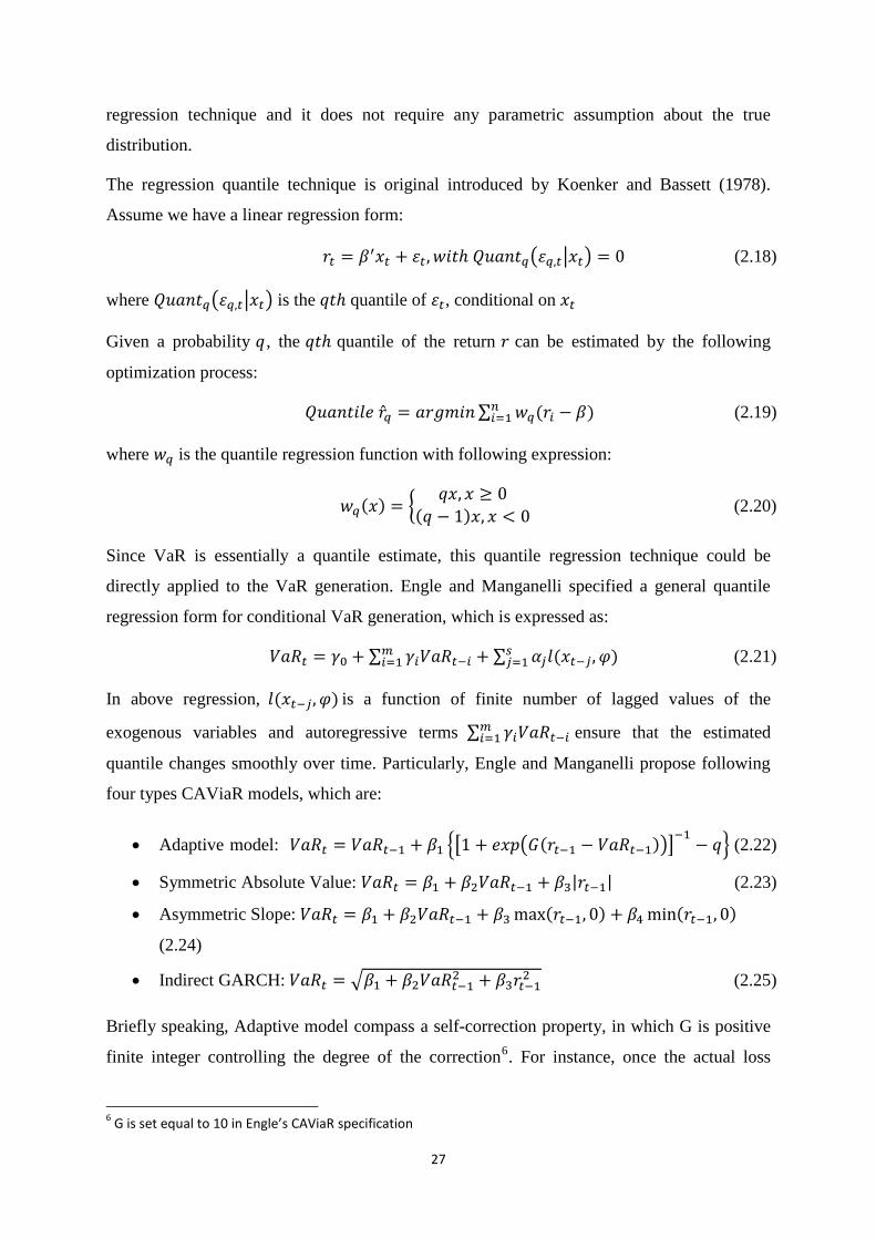
directly applied to the VaR generation. Engle and Manganelli specified a general quantile

regression form for conditional VaR generation, which is expressed as:

(2.21)

In above regression, is a function of finite number of lagged values of the

exogenous variables and autoregressive terms ensure that the estimated

quantile changes smoothly over time. Particularly, Engle and Manganelli propose following

four types CAViaR models, which are:

Adaptive model:

(2.22)

Symmetric Absolute Value: (2.23)

Asymmetric Slope:

(2.24)

Indirect GARCH:

(2.25)

Briefly speaking, Adaptive model compass a self-correction property, in which G is positive

finite integer controlling the degree of the correction6. For instance, once the actual loss

6 G is set equal to 10 in Engle’s CAViaR specification

28

exceed the VaR estimate in the last period, the second term of the adaptive model will

become positive which increase the VaR prediction in the next period and vice versa. The

symmetric and indirect GARCH model has mean reverting property and responds

symmetrically to the past returns. The asymmetric slope model, on the other hand, takes into

account the asymmetric effect of the returns on the risk prediction.

In fact, CAViaR can be more flexible than above four types of specifications. It can also be

applied to some nonlinear forms and non-iid distributed errors. Weiss (1991) shows the

consistency and asymptotic normality property of the nonlinear regression quantile

estimators, which could be served as the most critical contributions to the non-linear

regression quantile technique.

The only assumption required under the CAViaR framework is that the quantile regression is

correctly specified, which reduce the risk of misspecification of the error term distribution

under the parametric model. White (1994) shows that even if the the quantile regression is

misspecified, the minimization of the regression quantile objection function still satisfies the

Kullback-Leibler Information Criterion, which measures the discrepancy between the true

model and estimated one.

2.2 Combining risk exposure modeling with VaR models

The VaR models illustrated in the section 2.1 provides a quantitative measurement of the

downside risk of the underlying risk factors. In practice, however, the potential loss from a

financial position is attributed to two risk sources, which are:

The downside risk of the underlying risk factors (Measured by VaR models)

The risk exposure to these underlying risk factors.

From the perspective of portfolio manager, the downside risk from the underlying risk factor

is stochastic and outside their control because it is purely driven by the randomness of the

risk factor’s distribution. The risk exposure to the risk factor, which determined by the

magnitude of the portfolio position, could be cautiously chosen by the trader for active risk

management. The overall risk of the portfolio is obtained by combining the risk exposure

estimated from the portfolio position and the downside risk estimated from the VaR models.

Generally speaking, there are two approaches which could used to model the risk exposures,

which are Local-valuation approach and Full-valuation approach. Under Local-valuation

approach, the portfolio position is replaced by the linear or quadratic risk exposures using

29

partial derivatives. Full valuation approach, on the other hand, measure the risk exposure by

fully re-pricing the portfolio’s position over a range of new scenarios.

2.2.1 Local-valuation approach

The commonly used Local-valuation approach is the Quadratic Model by Wilson (1994). To

brief explain it, consider a portfolio whose value depends on the single risk factor and time t

(e.g.: a portfolio of options with the same underlying stock ). The value of this portfolio can

be expressed as a function of and as

Apply Taylor expansion7 we have:

(2.26)

where and are the first and second partial derivative respects to the portfolio value and

is the deterministic time drift.

Assume for assigned confidence level , the minimal acceptable portfolio value is achieved

when the value of underlying stock is equal to:

(2.27)

where is the initial value of the underlying stock at time 0, and are the same

parameters from the parametric VaR model (2.6).

Transform into VaR measure we have:

(2.28)

Apply Taylor expansion to the right side of (2.28) and ignore the time drift (since the position

only evaluate once at initial time), we have:

(2.29)

Equation (2.29) is the Quadratic Model and it is useful to model the risk exposure when the

portfolio consists of substantial derivative components with the same underlying risk factor.

On the other hand, if the portfolio is exposed to many risk factors, equation (2.26) will

become to:

(2.30)

7 Thomas, George B. Jr.; Finney, Ross L. (1996), “Calculus and Analytic Geometry”

30

where and are vector of N elements (If exits N risk factors) respectively, and is an N-

by-N symmetric matrix , in which the diagonal components are the gamma of the risk

factors and the off-diagonal terms are the cross-gammas, which is expressed as:

(2.31)

where and are and underlying risk factors

In fact, Solving (2.31) will become increasingly complex as number of the underlying risk

factors increase. For instance, if N = 50, 50 estimates of and 1275 estimates of the

covariance matrix need to be calculated.

Furthermore, for more complex function , it may not feasible to use (2.26) for VaR

transformation, since might not be monotonic. Take Variance operator to both sides of

(2.26) and ignore the time drift we have:

(2.32)

Assuming is normal distributed (e.g., represent the continuous stock return), then we

have:

(2.33)

Under normal distribution, the odd moments are zero. Substitute (2.33) into (2.32) and ignore

the last term we have:

(2.34)

Parametric VaR estimate is therefore given by:

(2.35)

where is the standard normal quantile.

The further improvement of equation (2.35) is so called Cornish-Fisher Expansion8 , in which

is replaced by , which is expressed as:

(2.36)

where measure the skewness of the portfolio’s distribution, which is computed as:

8 See John Hull (1997)

31

(2.37)

This adjustment provides a more generic quantile estimator compared to the standard normal

quantile. In fact, under the normality assumption, the estimate of will be zero according to

(2.40), making and indifferent. When a positive or negative skewness exists, the

accuracy of the VaR estimate should be increased under Cornish-Fisher Expansion.

To sum up, local value approach quantifies the risk exposure by valuing the portfolio once at

its initial position. Any possible future movement of the value is predicted using partial

derivatives to the underlying risk factor. Within this class, equation (2.29) and (2.35) could

be applied for linear or Quadratic approximation. The choice between these two equations are

depends on whether the portfolio payoff is monotonic.

2.2.2 Full-valuation approach

Although equation (2.35) provides a solution for the portfolio whose payoff is non-monotonic,

this equation is only works well under the assumption that the future movement of the

portfolio is not far from its initial point. In practice, the extreme value movement is exactly

what the risk manager care about. This raises the need of the full valuation. Under the full-

valuation approach, future values of the risk factors are generated by simulation technique.

For each realization of the risk factors, the portfolio is re-priced at the new scenario. The VaR

estimate is obtained as the percentiles of the full distribution of the re-priced payoffs over a

range of scenarios.

The accuracy of the full-valuation approach is highly depends on the pre-specified stochastic

process for the underlying risk factors. One commonly used stochastic process for random

value generation is Markov process by Russian mathematician Markov [See Everitt(2002)].

Consider a variable with a mean change of zero and a variance rate of 1.0 (Wiener process),

where:

where is the standard white noise (2.38)

The value of for any two different short intervals is independent

These two properties indicated that the uncertainty of the variable in the future, as measure

by its standard deviation, increase by the square root of the time .

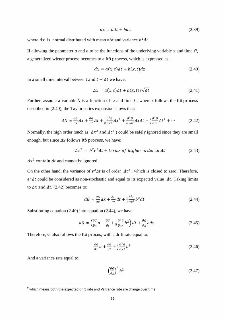
Generally, if let and to be the drift and the variance rate respectively, a generalized

Wiener process can be expressed as:

32

(2.39)

where is normal distributed with mean and variance

If allowing the parameter and to be the functions of the underlying variable and time 9,

a generalized wiener process becomes to a , which is expressed as:

(2.40)

In a small time interval between we have:

(2.41)

Further, assume a variable is a function of and time , where follows the

described in (2.40), the Taylor series expansion shows that:

(2.42)

Normally, the high order (such as ) could be safely ignored since they are small

enough, but since follows , we have:

(2.43)

and cannot be ignored.

On the other hand, the variance of is of order , which is closed to zero. Therefore,

could be considered as non-stochastic and equal to its expected value . Taking limits

to and , (2.42) becomes to:

(2.44)

Substituting equation (2.40) into equation (2.44), we have:

(2.45)

Therefore, G also follows the , with a drift rate equal to:

(2.46)

And a variance rate equal to:

(2.47)

9 which means both the expected drift rate and VaRiance rate are change over time

33

Denote and , the stochastic process followed by the stock prices can

be expressed as:

(2.48)

In a small time interval between we have:

(2.49)

Given that the stock price follows the (2.49), the logarithm of the stock should

follow with following form according to equation (2.46) and (2.47):

(2.50)

The change of between time 0 and time T is therefore normally distributed with:

(2.51)

Take integral of equation (2.51) we have:

(2.52)

where

Equation (2.52) is the general stochastic process to simulate the random stock price over

interval . At discrete time step , we have:

(2.53)

If we assume is not constant over time and model it by GARCH process, Hull (2008)

shows another stochastic process for the dynamic evolution of , which is expressed as:

(2.54)

where and are the parameters estimated from GARCH model (2.7) and is the long-

term variance.

The speed of the convergence to the long-term volatility in the process (2.54) depends on

the persistence parameters ( ) in GARCH model. Empirical study shows that typically

the financial series have GARCH persistence around 0.95-0.99 for daily volatility. Under

such condition, the simulated volatility using (2.54) will be pulled back to its long-run

average within 1 month approximately.

34

Combining the stochastic processes (2.52) and (2.54), we could simulate thousands of

realized value of the underlying stock . After re-pricing the portfolio at the each scenario,

VaR can be estimated from the percentile of the full re-priced distribution.

The Monte Carlo simulation could accounts for nonlinearities and time decay effect of the

underlying risk factor to the value of the target portfolio. (e.g.: a portfolio of call options with

different maturity), which will generate a more accurate risk measure than local-valuation

approach. On the other hand, Full-valuation approach requires substantial computing time.

For instance, if we generate 10,000 value of the underlying risk factor, we have to re-price

the portfolio 10,000 times before calculating the corresponding VAR. Besides, the accuracy

of full-valuation approach also highly depends on the pre-specified underlying stochastic

process. As shown by Jorion(2006), if the underlying process is inappropriate specified, the

estimated risk might be deviated from the true one.

2.3 Risk decomposing by VaR models

VaR models are more than just estimation of the overall market risk of the target portfolio.

From the perspective of active risk managers, single VaR estimate might not be sufficient

because it cannot tell the trader which component position in the portfolio contributes most of

the risk and how to adjust the individual position in the portfolio to reduce the overall market

risk. Combining with Modern Portfolio Theory, on the other hand, VaR could decompose the

risk of the overall portfolio down to the some individual parts, which provides fairly useful

information for the active risk management.

2.3.1 Marginal VaR

One useful risk measure decomposed from VaR is the marginal VaR. Marginal VaR (MVaR)

can be derived from Markowitz’s Modern Portfolio Theory [See Edwin and Martin (2009)].

By definition, MVaR is the change of the portfolio VaR resulting from taking an additional

cash exposure to a given component, which is expressed as:

(2.55)

where is the initial amount of the investment in the portfolio and is the weight of the

individual asset in the portfolio. If VaR is estimated by parametric model, equation (2.55)

could be re-write as:

(2.56)

35

Above transformation indicated that the MVaR is closely related to the asset beta in CAPM

model.

Using matrix notation, the vector in CAPM model can be written as:

(2.57)

where is the weight vector and is the covariance matrix

Combining equation (2.56) with (2.57) , MVaR can be written related to i as:

(2.58)

MVaR provide user the marginal risk for each position contributed to the overall portfolio.

Risk manager could therefore use it to decide the appropriate rebalancing plan of the

portfolio’s position to reach the optimal risk level.

In fact, the optimal risk level implied by MVaR is consistent with the statement in CAPM

model. The role of the portfolio manager is to choose a portfolio that represents the best

combination of return and risk based on the modern portfolio theory. The object function is to

maximize the Sharpe ratio (1966), which is:

(2.59)

At the optimal point, the ratio of any expected excess return from individual asset to its

MVaR must be equal, that is:

(2.60)

Equation (2.60) implied that for any efficient portfolio, the expected return on any component

asset must be proportional to its beta relative to this portfolio, this is:

(2.61)

where is the expected excess return from market portfolio

This condition is exactly consistent with CAPM.

2.3.2 Incremental VaR and best hedge ratio

Incremental VaR (IVaR) is proposed by J.P. Morgan (2008). It is another useful risk measure

separated from the overall VaR measure, which provide the risk manager useful information

about the best hedge ratio. By definition, Incremental VaR is the change in VaR owing to a

36

new position. It differs from the marginal VaR in that the amount added or subtracted can be

large, which cause VaR changes in a more nonlinear fashion. Incremental VaR can be

approximated by Marginal VaR, which can be expressed as:

(2.62)

where is the amount of investment added to the current position of assets .

Assume the amount is added to only one asset, the variance of the cash return on the new

portfolio can be expressed as:

(2.63)

where and are the cash value of the portfolio before and after amount is added.

To find the lowest portfolio risk, differentiating the equation (2.63) with respect to and set

its value equal to zero. This number could be regarded as the best hedge ratio, which is

expressed as:

(2.64)

This measure tells the risk manager how much the additional amount to invest in an asset so

as to minimize the overall risk of the portfolio.

As proposed by Riskmetrics, IVaR reflects the dynamic of the correlations amongst all

individual positions that compose the target portfolio. As the risk manager remove the certain

individual position and calculate its IVaR, he is able to assess the significant of the

interaction of that position with the rest of the assets in the target portfolio. This information,

however, cannot be reflected by the simple correlation coefficient estimated from the original

covariance matrix, which only provides a static and statistical relationship.

2.4 Risk integration techniques

Modern risk management requires applying VaR measures on the portfolios with high level

of diversification. These portfolios might include large number of stocks, bonds, commodities,

currencies and derivatives. If every position in the portfolio is modeled individually using

VaR models explained in the above sections, the risk modeling procedure will become

considerably complex and time intensive. For instance, if the portfolio contains individual

assets, we have to estimate

numbers of the parameters to decide the full covariance

matrix used by VaR measures. If the number of the sample observations is less than

37

number of assets in the portfolio, negative value of the portfolio variance may be obtained,

which makes no sense for VaR calculation.

The best way to solve the risk aggregation problem is to integrate the portfolio risk using risk

mapping techniques, in which the individual positions in the portfolio are substituted by a

small number of the selected risk factors. This summarization technique could considerable

improve the speed of the portfolio risk modeling without losing much accuracy.

2.4.1 Regression analysis

We introduce two commonly adopted risk mapping approaches in this section, which are

regression analysis and Principle Component Analysis. In the case where the risk factors

could be decided in advance, regression analysis could be applied to ascertain the risk

exposure. For instance, CAPM states that the return of the individual stock is driven by the

systematic risk from the market index. We could therefore estimate the risk exposure by

running a regression of the stock returns against the market index return.

The Diagonal Model by Sharpe (1966) could be treated as a simple regression analysis for

risk mapping. Under the diagonal model, the common movement of the individual stock

return is captured by the movement of the market index return , which can be expressed

by a simple regression as:

(2.65)

where is the parameter called factor loading, is the white noise

The variance of the individual stock therefore can be decomposed using (2.65) as:

(2.66)

The full covariance matrix of the portfolio becomes to:

(2.67)

where is the diagonal matrix of residual ’s variance and is vector of all factor

loading

Applying (2.67), the variance of the portfolio could therefore be expressed as:

(2.68)

where is the weight vector

38

Similarly, all future or option positions with same underlying asset but different maturities

could be mapped to the risk factor represented by the underlying asset; all bonds positions

with different coupon rates and maturities could be mapped to the risk factor represented by

the yield change risk (duration model). The transformation using regression analysis could

considerably simplify the estimation of the overall portfolio’s risk. For instance, given the

portfolio contains individual stocks, the number of the parameters need to estimated

is

when using full matrix valuation. Using diagonal model (2.68), on the other hand,

the number of the parameters could be reduced to only .

2.4.2 Principle Component Analysis

More generally, Principal Component Analysis (PCA) can be used to find a series of

independent linear combinations of the risk factors that provided the best explanation of the

original covariance matrix of the portfolio. This is a mathematical procedure invented by

Pearson (1901), which involves using orthogonal transformation to convert a set of

observations of possibly correlated variables into a set of values of uncorrelated variables.

Jorion (2006) applied this method into the risk modeling. Assuming the principal component

is a linear combination of the individual assets’ returns in the portfolio, which is expressed

as:

(2.69)

where and are vector expression

We have:

(2.70)

where is the covariance matrix of

Set the normalization constraint on the norm of the factor exposure vector, which is:

(2.71)

Under this constraint, becomes the Eigen-value of the covariance matrix and is its

associated eigenvector, which is expressed as:

(2.72)

For each , it is associated with an Eigen-value equal to . If we sort the variance

39

in decreasing order and keep the first components (beyond which their

variances is small and unimportant), we have:

(2.73)

and

(2.74)

We could therefore re-write the portfolio return as:

(2.75)

In this way, the overall risk exposures of the portfolio can be mapped to k principal

components ( ). Since each risk factor is independent, the variance of the

portfolio could be estimated as:

(2.76)

The PCA is particularly useful in the case when the risk factors could not possible be decided

in advance. For instance, if the portfolio consists of different class of assets, we could apply

PCA to determine several principal risk factors and thereby replace the whole portfolio risk

by the smaller number of the selected PCAs.

2.5 Risk overlay on multi-time horizon

The above literature view considers nothing about the time horizon setting of the risk forecast

(daily VaR estimate is set by default). However, it is unrealistic to assume that the investor’s

portfolio will only be frozen for a single day. In practice, there is also a important concern of

the multi-day horizon risk forecast for the risk managers and regulators (e.g.: Basel II require

Bank to reports 10 days VaR on 99% confidence level, based on their outside-investment

position).

40

We present several feasible approaches for the multiday risk forecast in this section.

Particularly, we consider an idea of generating multiday-VaR prediction by directly fitting

the historical VaR series into pre-specified time series model. The dynamic risk model

proposed in chapter four is exactly derived from this idea.

2.5.1 Factors considered in the VaR models

From the perspective of risk managers, VaR can be viewed as either the maximum loss at

normal market condition or the minimum loss at extreme market condition, given certain

confidence level and time horizon. This measure is popularly used as a criterion for

appraising the market risk or setting capital cushion by the regulators, which ensure the

financial institutions could still operate after some catastrophic events. In practice, VaR

modeling involves dealing with several quantitative factors, which are:

Confidence level

Data frequency

Cumulative Density Function

Mark to market value

Among these factors, Cumulative Density Function of the return’s distribution the central

consideration. To see this, define a long position’s VaR for holding period at confident

level as:

(2.77)

where is the changes of the portfolio value over holding period

For short position, it becomes:

(2.78)

It is clearly that the Multi-day VaR estimate for long position is derived from left tail of the

, while the Multi-day VaR estimate for short position is derived from right tail of the

.

2.5.2 Multi-day VaR from IGARCH model

To derive the conditional distribution of the return series, we first consider the parametric

VaR model proposed by Peter (1996), in which the continuous compounding daily return is

assumed to be conditional normal, which is expressed as:

41

(2.79)

where and are the conditional mean and variance at time

Assume the dynamicity of is modeled by IGARCH (GARCH with no drift) process,

which is expressed as:

(2.80)

This special type of GARCH model is equivalent to the Exponential Weight Moving Average

(EWMA) process. Substituting the top equation in (2.80) into the bottom equation, we have:

(2.81)

This could be generally expressed as:

(2.82)

Taking the conditional expectation to both sides of equation (2.82) and notice that:

(2.83)

We have:

(2.84)

Equation (2.84) shows that in IGARCH model, the -day conditional variance is equal to:

(2.85)

Therefore the -day conditional distribution of the continuous compounding return follows

normal distribution, which is expressed as:

(2.86)

The -day VaR becomes:

(2.87)

where is the cash amount of portfolio and is the quantile from standard normal

distribution.

Equation (2.87) is so called the time-square root rule under the Risk-Metrics system and it’s

fairly easy to implement in the multiday VaR forecast. Given that the financial assets always

42

have fatter tails, could be replaced by student quantile for a more conservative

measurement.

Note that the equation (2.87) only valid under the assumption that returns follow IGARCH

process. If there is a drift term in either the return or volatility process described in equation

(2.80), time square root rule could be broken down. For instance, consider a return process

with a drift term, which is:

(2.88)

This could be a case when the assets could provide a non-zero unconditional expected return.

As shown by Tsay (2005), the assumption is particularly hold for some high-frequency traded

securities. The distribution of the -day return changes to:

(2.89)

The -day VaR will changes to:

(2.90)

2.5.3 Multi-day VaR from ARMA-GARCH model

The multi-day VaR for an ARMA-GARCH model could be derived in a similar way. To see

this, consider the following time series model for return and conditional variance :

(2.91)

In above model, the return follows ARMA process while the conditional variance

follows GARCH process. If the model specification is correct, should follows a standard

Gaussian process with elliptical distribution. For given information on time , should

have the same conditional distribution as , which is expressed as:

(2.92)

where and can be estimated from equation (2.91).

A common assumption for the distribution of could be normal or student . 1-day VaR of

therefore could be expressed as:

43

(2.93)

where is the quantile of the with degree of freedom

For the -day VaR, we need to forecast and using model (2.91).

To simply the forecast, we transform the ARMA process (2.91) into a purely infinite MA

model, which is expressed as:

(2.94)

At the initial time , the -day ahead forecast of using (2.94) could be expressed as:

(2.95)

Since for any , is hold. (2.95) could be simplified as:

(2.96)

The corresponding forecasting error from (2.96) is equal to:

(2.97)

The total error of -day ahead forecast is the sum of the forecasting error from 1 day to -day,

which is:

(2.98)

where

The -day ahead volatility forecast at initial date is therefore given by:

44

(2.99)

where is the conditional variance estimated by the GARCH process 2.91

Consider a special case where follows an AR-GARCH (1, 1) process, where:

(2.100)

Since tr follows an MA (1) process, the -day ahead return forecast is just equal to .

The corresponding total error is equal to:

(2.101)

Using GARCH (1, 1) process, a forecast variance over -day equal to:

(2.102)

Apply iteration to and (2.102) combine with (2.99), we have:

(2.103)

If is standard normal distributed, the conditional distribution of is normal as well,

that is:

(2.104)

The -day holding period VaR could be therefore expressed as:

(2.105)

where could be estimated from equation (2.103)

2.5.4 An ideal of accuracy improvement

The above section illustrates how to derive the multiday conditional CDF from an ARMA-

GARCH model. Virtually speaking, the longer the forecast period by a single time series

model, the greater the forecast error occurs. A theoretical way to overcome this problem is to

frequently re-estimate the model’s parameters using the latest historical data. For example,

45

assume we wish to estimate 10-day variance at the initial date , we could re-estimate the

GARCH model frequently , in which the fixed data window moves one day forward at each

re-estimated time. Since each model parameters provides only daily variance forecast, the

overall variance is the sum of the ten daily variance forecast. Statistically, if we re-estimate

the model times with the fixed window length, the total forecast error over day is equal to :

(2.106)

Note that we remove the filtration in above formula because the information set is updated

for each estimated value.

One limitation of this procedure is that it could only be applied to the historical data, because

we have to wait until tomorrow to know the new information in the data window to re-

estimate the model. This is obviously not feasible in practice (For instance, if we want

estimate a 10-day VaR from today, we have to wait for 9 days to obtain all required

information ).

This problem could be solved, however, if we can find an appropriate time series model to

directly model the historical Multi-day VaR series. Once the time series model has been

appropriate specified, we could estimate the parameters based on the historical multi-day

VaR series and generate a VaR forecast. This idea is the exactly the motivation of the

Dynamic risk model we proposed in the chapter four.

2.6 Conclusion

This Chapter provides a general introduction of Value at Risk models and its evolution in the

financial risk measurement. To be specific, Section one provides a formal definition of VaR

and its statistical foundation. We show how VaR could be estimated using parametric, non-

parametric and semi-parametric approach separately. The key difference of these approaches

lies in the different ways of the return distribution modeling. The pro and cons of each model

is briefly discussed as well. We also discuss the issue of time varying conditional distribution

in the VaR modeling. Two general approaches are presented, in which one is focus on the

dynamic adjustment of the conditional volatility and the other is focus on the dynamic

adjustment of the conditional quantile. However, there is currently no agreement on which

46

approach is superior since there is no quantitative approach available to separate these two

effects on the time varying conditional distribution.

While the section one focus on the VaR modeling of the underlying risk factors, the next two

sections turn to the risk measurement for portfolios. Given the fact that the market risk of the

portfolios is driven not only by the VaR of the underlying risk factors but also by the risk

exposure to these underlying risk factors, we explain two useful approaches for risk exposure

modeling. The risk mapping approaches represented in the following section, on the other

hand, could be applied to determine appropriate underlying risk factors.

In the final section of this chapter, we provide the derivation of the multi-day VaR forecast in

the context of ARMA process. This includes the time squared root rule from the IGARCH

process and the general formula from the ARMA-GARCH process. Furthermore, we point

out an idea that if we could find an appropriate model to fit the historical VaR series, the

accuracy of the VaR forecast will possibly be improved compared to the traditional

approaches.

47

3 Application of VaR models in the financial market risk measurement

Followed by the market risk modeling techniques presented in chapter two, this chapter

implements a complete model application based on several hypothetical portfolios,

constructed on both historical and simulated data. The purpose of running this application is

to demonstrate the pros and cons of each selected model through empirical analysis, which

set the scene for the development of new VaR methods in chapters four and five.

Particularly, we are attempting to address three main issues through model application, which

can be summarized as following:

Compare the performance of VaR models under different asset classes (e.g.: equities,

bonds, options and futures) and select the most appropriate VaR model for each class.

Analyze the feasibility of two dynamic adjustment approaches through back-testing.

Implement two risk mapping techniques into the portfolio risk simplification process

and formulate some useful selection criterions

Model application also provides us a comprehensive and deep understanding of the practical

use of VaR models and thereby contributes to some possible model innovations in the further

PhD research.

3.1 Dataset

Hypothetical portfolios constructed in this chapter consist of stocks, bonds, currencies and

their derivatives. All historical data are collected from Thomson Reuters DataStream and

covered both the US and the UK financial market. More specifically, equity data are range

from six major sectors of industry center, which are:

1. Communication Equipment

2. Major Airlines

3. Industrial Metals Minerals

4. Electric Utilities

5. Money Center Banks

6. Auto Manufacturers

From each sector, three largest companies and three smallest companies are chosen based on

their market capitalization. In overall, the dataset consist stocks of thirty-six companies listed

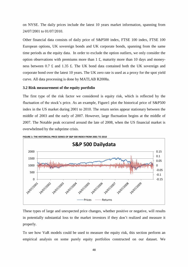
48

on NYSE. The daily prices include the latest 10 years market information, spanning from

24/07/2001 to 01/07/2010.

Other financial data consists of daily price of S&P500 index, FTSE 100 index, FTSE 100

European options, UK sovereign bonds and UK corporate bonds, spanning from the same

time periods as the equity data. In order to exclude the option outliers, we only consider the

option observations with premiums more than 1 £, maturity more than 10 days and money-

ness between 0.7 £ and 1.35 £. The UK bond data contained both the UK sovereign and

corporate bond over the latest 10 years. The UK zero rate is used as a proxy for the spot yield

curve. All data processing is done by MATLAB R2008a.

3.2 Risk measurement of the equity portfolio

The first type of the risk factor we considered is equity risk, which is reflected by the

fluctuation of the stock’s price. As an example, Figure1 plot the historical price of S&P500

index in the US market during 2001 to 2010. The return series appear stationary between the

middle of 2003 and the early of 2007. However, large fluctuation begins at the middle of

2007. The Notable peak occurred around the late of 2008, when the US financial market is

overwhelmed by the subprime crisis.

FIGURE 1: THE HISTORICAL PRICE SERIES OF S&P 500 INDEX FROM 2001 TO 2010

These types of large and unexpected price changes, whether positive or negative, will results

in potentially substantial loss to the market investors if they don’t realized and measure it

properly.

To see how VaR models could be used to measure the equity risk, this section perform an

empirical analysis on some purely equity portfolios constructed on our dataset. We

-0.15

-0.1

-0.05

0

0.05

0.1

0.15

0

500

1000

1500

2000

S&P 500 Dailydata

Prices Returns

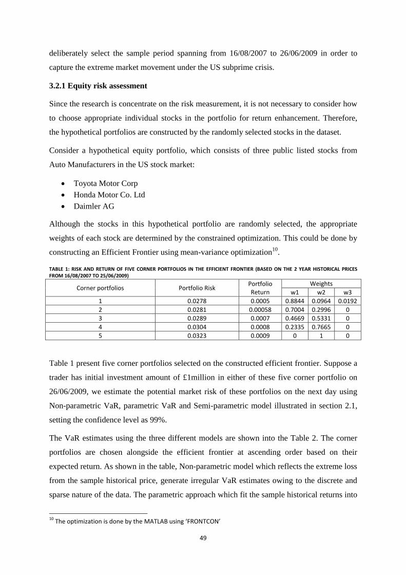
49

deliberately select the sample period spanning from 16/08/2007 to 26/06/2009 in order to

capture the extreme market movement under the US subprime crisis.

3.2.1 Equity risk assessment

Since the research is concentrate on the risk measurement, it is not necessary to consider how

to choose appropriate individual stocks in the portfolio for return enhancement. Therefore,

the hypothetical portfolios are constructed by the randomly selected stocks in the dataset.

Consider a hypothetical equity portfolio, which consists of three public listed stocks from

Auto Manufacturers in the US stock market:

Toyota Motor Corp

Honda Motor Co. Ltd

Daimler AG

Although the stocks in this hypothetical portfolio are randomly selected, the appropriate

weights of each stock are determined by the constrained optimization. This could be done by

constructing an Efficient Frontier using mean-variance optimization10

.

TABLE 1: RISK AND RETURN OF FIVE CORNER PORTFOLIOS IN THE EFFICIENT FRONTIER (BASED ON THE 2 YEAR HISTORICAL PRICES FROM 16/08/2007 TO 25/06/2009)

Corner portfolios Portfolio Risk Portfolio Return

Weights

w1 w2 w3

1 0.0278 0.0005 0.8844 0.0964 0.0192

2 0.0281 0.00058 0.7004 0.2996 0

3 0.0289 0.0007 0.4669 0.5331 0

4 0.0304 0.0008 0.2335 0.7665 0

5 0.0323 0.0009 0 1 0

Table 1 present five corner portfolios selected on the constructed efficient frontier. Suppose a

trader has initial investment amount of £1million in either of these five corner portfolio on

26/06/2009, we estimate the potential market risk of these portfolios on the next day using

Non-parametric VaR, parametric VaR and Semi-parametric model illustrated in section 2.1,

setting the confidence level as 99%.

The VaR estimates using the three different models are shown into the Table 2. The corner

portfolios are chosen alongside the efficient frontier at ascending order based on their

expected return. As shown in the table, Non-parametric model which reflects the extreme loss

from the sample historical price, generate irregular VaR estimates owing to the discrete and

sparse nature of the data. The parametric approach which fit the sample historical returns into

10

The optimization is done by the MATLAB using ‘FRONTCON’

50

normal distribution, generate smoother VaR estimates with ascending order. Besides, the

parametric VaR provides a lower VaR prediction than non-parametric approach as the

portfolio become risky, indicating that it assigns relatively low probability to the extreme

events. The EVT semi-parametric approach, on the other hand, provides both smooth and

relatively high value of the VaR estimates.

TABLE 2: COMPARISON RESULTS OF THREE SELECTED VAR APPROACHES ON 26/06/2009

CORNER

PORTFOLIOS IN

EFT(FROM LOW

TO HIGH

EXPECTED

RETURN

Non-

Parametric

VaR (£)

Parametric

VaR (£)

Semi-parametric VaR

Portfolio

Absolute

Return 1 day

after(£) VaR (£) Shape

parameter Scale

parameter

1 75625 64749 77987 0.2247 0.0146 55201

2 74902 65313 78865 0.1888 0.0158 55115

3 76140 67331 82683 0.1215 0.0188 64326

4 79118 70704 86589 0.1365 0.0192 70324

5 85100 75251 88004 0.1177 0.0210 76115

Figure 2 plot the histogram, normal distribution and EVT tail distribution drawn from the

sample historical returns of the first corner portfolio (Assuming the loss is positive hence we

focus on the right tail). As shown in the figure, both normal (white line) and EVT (green line)

tail has smoother shapes than the histogram. On the other hand, the histogram shows certain

level of extreme outliers, which will be underestimated if using normal distribution as

approximation.

FIGURE 2: HISTOGRAM, NORMAL DISTRIBUTION AND EVT TAIL DISTRIBUTION OF THE FIRST CORNER PORTFOLIO USING 2 YEAR HISTORICAL PRICES FROM 16/08/2007 TO 25/06/2009

Comparing the actual loss on the next day with the VaR estimates (see the last column of

table 1), it can be seen clearly that the actual loss of the fifth portfolio (£76115) violate the

parameter VaR estimate (£75251), while in other situations, the three VaR models could

generate a sufficient VaR estimate to capture the realized loss.

51

VaR can be interpreted as a measure of the maximum potential loss under the normal market

condition or minimum potential loss under the extreme market condition. Jorion (2006)

pointed out that the selection criterion of the VaR models is ambiguous in the literature

(whether parametric, non-parametric and semi-parametric). The risk manager might choose

VaR models based on the overall market condition. For instance, if the market is normal

volatile, they tend to choose parametric VaR because it easy to implement and the result can

be calculated quickly. If the market is current highly fluctuated, they might use semi-

parametric VaR because it could more accurately capture the extreme tail risk and provide a

more conservative risk estimate.

However, the above empirical result seems indicates that rather than the overall market

condition, the risk degree of the target portfolio should be the key consideration when select

the VaR models. To be specific, given the moderate portfolio risk level, parametric VaR

could generate a sufficient risk estimate even the market is at high volatility regime (as the

sample period we chosen). However, as we move alongside the efficient frontier and

increase the risk degree of the corner portfolio, Parametric VaR estimates become less

reliable and it is eventually broken by the actual loss at the fifth corner portfolio. Semi-

parametric VaR is preferable for these kinds of high risky portfolios.

It also necessary to mention that these VaR models are all based on the conditional

distribution derived from the sample historical data. These measurements might be unreliable

if the actual distribution in the next day derived far from the sample historical data. (e.g.:

Regime switch occurs)

3.2.2 Risk integration of the equity portfolio

Besides the risk degree of the target portfolio, we also like to consider the effect of the scale

of the target portfolio to the VaR estimates. Because as the number of the individual stocks in

the portfolio increase, the input parameters in the VaR models will increase as well, which

increase the cost and complexity of the estimation as well.

For a research, we construct a large hypothetical portfolio consisting of all 36 selected stocks

in the dataset to examine how the scale problem will affects the speed and accuracy of the

VaR estimate. Since the weight of the individual asset is non-stochastic in the process of

52

VaR estimation11

, we fix the equal weights of the individual stocks in the portfolio and

perform the analysis.

Table 3 shows the result of the VaR estimates of the hypothetical portfolio. The parametric

VaR (in the second column) is obtained by fully estimated the covariance matrix of 36

individual stocks. Along with this, we also estimated VaR using two risk mapping

approaches, which are diagonal model and PCA (Detailed Risk mapping techniques are

explained in Chapter 2.4).

TABLE 3: THE PORTFOLIO VAR ESTIMATES USING PCA AND DIAGONAL MODEL ON 26/06/2009 (AT 5% VAR CONFIDENCE LEVEL)

Parametric VaR

(Full Covariance Matrix)

VaR using risk mapping technique

Diagonal Model PCA analysis (16 PCAs)

VaR 39358millon£ 38089millon£ 39235million£

Computation Time 1.05sec 0.01sec 0.023sec

Portfolio Actual Loss next day on 2009/6/27 21016million £

Focusing on the Table 3, the differences of the VaR estimates generated from these three

approaches are not substantial, given that the initial investment amount is £1million. Among

these, VaR estimate using full covariance matrix (without using mapping approach) generates

the highest estimate value with the longest computation time. This is understandable since

full valuation of the covariance matrix takes into account the full price information of each

individual stock in the portfolio, with the total number of the parameters equal to (

). On the other hand, two risk mapping approaches only consider the effect of the certain

common risk factors obtained from the mapping technique. This simplification results in a

slightly lower VaR estimates but a considerable improvement of the computation time. We

expected that the time reducing effect due to the parameter reducing should be more

significant if the trader’s portfolio contained hundreds of individual positions.

11

The target portfolio is assume to be frozen when estimate the VaR

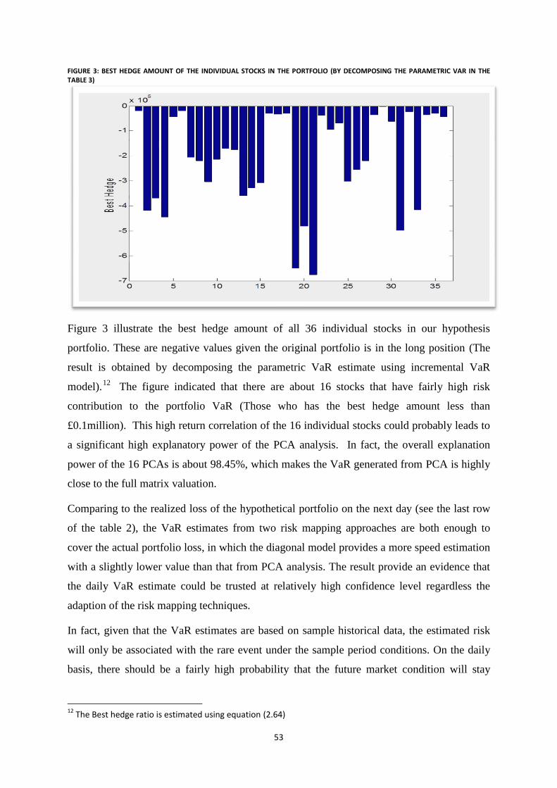
53

FIGURE 3: BEST HEDGE AMOUNT OF THE INDIVIDUAL STOCKS IN THE PORTFOLIO (BY DECOMPOSING THE PARAMETRIC VAR IN THE TABLE 3)

Figure 3 illustrate the best hedge amount of all 36 individual stocks in our hypothesis

portfolio. These are negative values given the original portfolio is in the long position (The

result is obtained by decomposing the parametric VaR estimate using incremental VaR

model).12

The figure indicated that there are about 16 stocks that have fairly high risk

contribution to the portfolio VaR (Those who has the best hedge amount less than

£0.1million). This high return correlation of the 16 individual stocks could probably leads to

a significant high explanatory power of the PCA analysis. In fact, the overall explanation

power of the 16 PCAs is about 98.45%, which makes the VaR generated from PCA is highly

close to the full matrix valuation.

Comparing to the realized loss of the hypothetical portfolio on the next day (see the last row

of the table 2), the VaR estimates from two risk mapping approaches are both enough to

cover the actual portfolio loss, in which the diagonal model provides a more speed estimation

with a slightly lower value than that from PCA analysis. The result provide an evidence that

the daily VaR estimate could be trusted at relatively high confidence level regardless the

adaption of the risk mapping techniques.

In fact, given that the VaR estimates are based on sample historical data, the estimated risk

will only be associated with the rare event under the sample period conditions. On the daily

basis, there should be a fairly high probability that the future market condition will stay

12

The Best hedge ratio is estimated using equation (2.64)

54

similar to the sample period market condition. This could possibly explain why the daily VaR

estimates could be safety no matter which mapping technique is used for simplification.

Even so, the VaR estimates has limitations in that it may not include the extreme but

plausible scenarios that do exist in the reality. This explains why the risk manager required

some complementary tool such as stress testing to increase the security of the risk

measurement system.

3.2.3 Time varying conditional distribution on VaR estimates

As we mentioned in the end of the section 3.2.1, VaR models are based on the sample

historical data, these measurements could be unreliable if the actual distribution in the future

derived far from the distribution estimated from the sample. We now consider how the time

varying conditional distribution will affect the market risk estimates from VaR models.

Particularly, we consider the dynamic adjustment approach proposed by McNeil and Frey

(2000).It is a semi-parametric approach combining Extreme Value Theory and GARCH

model.

Assume the stock return follows a stochastic process with drift rate and variance rate ,

its value on day can be expressed as:

(3.1)

Where is the innovation at time

If the volatility is modeled by GARCH process, the innovation series (standard

residuals) from (3.1) can be extracted as:

(3.2)

The tail distribution of these standard residuals can be modeled by EVT. The form of the tail

estimator for Cumulated distribution function )(ˆ zF is given by:

(3.3)

Inverting the tail estimator formula (3.3), we have:

(3.4)

The conditional VaR ( quantile) could hence be calculated as:

55

(3.5)

Where and are estimated from GARCH model

We implement the model (3.5) to model the dynamic risk evolution of the FTSE100 index.

Figure 4 lot the daily price and its corresponding returns of FTSE 100 index from 2001 to

2010. The returns series reflect the overall equity market condition of the UK financial

market during the sample period. The significant volatility clustering effect in the return

series (red line) indicates that GARCH process could be appropriately chosen.

FIGURE 4: THE DAILY HISTORICAL PRICE SERIES OF FTSE 100 INDEX FROM 2001 TO 2010

We estimate the conditional volatility series of the FTSE 100 index using three GARCH

types of Model, including GARCH , EGARCH and GJR GARCH . The

extracted conditional volatility series are plotted against the market implied volatility, as

shown in figure 5.

56

FIGURE 5: CONDITIONAL VOLATILITY SERIES OF FTSE 100 INDEX EXTRACTED FROM THE TREED SELECTED GARCH MODELS (BLUE LINE: EGARCH. GREEN LINE:GJR-GARCH. BLACK LINE:GARCH )

We combine the GJR-GARCH volatilies with the tail estimator (3.4) for a time varying VaR

estimates (denote GJR semi-parametric VaR). To be specific, we obtained the time varying

VaR series by multiplying the conditional volatility series generated from the GJR-GARCH

model with the residual quantile estimated from EVT tail estimator (3.4). The conditional

Daily VaR series is shown in figure 6.

FIGURE 6: CONDITIONAL VAR FORECAST SERIES OF FTSE100 FROM 07/05/2009 TO 31/07/2010

For comparison purpose, we also produce other two types of VaR series, which are from:

GJR-normal: time varying VaR series generate by combining GJR-GARCH volatility

and standard normal quantile.

HS-VaR: VaR series generate from pure historical quantile

50 100 150 200 250 300 350 400 450

1

2

3

4

5

6

7

Volatility Surface

ConditionalVolatility using EGARCH

ImpliedVol surface

ConditionalVolatility using GJR-Asysmetric GARCH

ConditionalVolatility using UGARCH

07/05/0926/06/0915/08/0904/10/0923/11/0912/01/1003/03/1022/04/1011/06/1031/07/10-4

-3

-2

-1

0

1

2

3

4

5

6FTSE100 5% VaRs(100x)

Returns

HSVaR

GJR Normal

GJR Semi-parametric

07/05/0926/06/0915/08/0904/10/0923/11/0912/01/1003/03/1022/04/1011/06/1031/07/10-6

-4

-2

0

2

4

6FTSE100 1% VaRs(100x)

Returns

HSVaR

GJR Normal

GJR Semi-parametric

57

To evaluate the performance of the VaR estimates, we summarize the number of the violation

days during the sample period13

. The result is shown in Table 4. Focus on the third and fourth

column of the table, the VaR series (generating from both GJR normal and GJR semi-

parametric) provide more consistent and efficient predictions of the actual risk than the VaR

estimates from historical Quantile.

TABLE 4: BACK-TESTING RESULTS (COMPARE VAR SERIES WITH FTSE100 ACTUAL RETURNS FROM 07/05/2009 TO 31/07/2010)

VaR approaches Total sample

observations

Actual Violation at 95%

Confidence level

Actual Violation at 99%

Confidence level

Historical Quantile 325 17 5.2% 6 1.8%

GJR normal 325 14 4.3% 3 0.9%

GJR semi-parametric 325 14 4.3% 2 0.6%

The above empirical results indicate that the dynamic VaR series generated from GARCH

types of volatility perform fairly well in capturing the time varying risk evolution. Given the

conditional volatility series obtained from the GARCH process, we believe that this result is

not just obtained by a random chance.

To be specific, the conditional volatility series in the figure 5 shows that the GARCH types of

models could generate a similar volatility forecast as the market implied volatility (red line).

Since the implied volatility captures the market expectation of the risk due to its forwarding

looking property, this indicates that the VaR estimated from GARCH types of volatility is

fairly consistent with the market expectation.

Even the figure 5 shows that GARCH model might generate a lower volatility forecast than

that from the market subjective expectation at some occasion, the conditional VaR could still

be safety, because the quantile multiplier which captured the extreme risk at the normal

market condition could be served as a complement.

Furthermore, given the negligible pattern difference from the GJR normal VaR and the GJR

semi-parametric VaR at 5% significant level, our empirical result also indicate that if the time

varying distribution has already been considered by the time varying volatility (as modeled

by GARCH types of model), the time varying quantile have limited effect on the VaR

estimates at relatively low confidence level. Therefore, although McNeil and Frey advocated

that standard normal quantile are likely to underestimate of the tail risk compared to EVT,

this empirical result shows that that underestimate problem tends to disappear at lower

confidence level(say 95% confidence level ), as long as the dynamicity is generated from the

GARCH types of volatility. 13

The violation day is defined as the day when actual return fall below the estimated VaR

58

Indeed, this conclusion may not be comprehensive, since the research has not verified the

statement through various types of financial data and the time horizon selection is relatively

short. However, it does provide us a useful implication to improve the dynamicity of VaR

estimates, which states that the time varying quantile effect could be partly captured by the

time varying volatility when implement the risk modeling technique. The dynamic CAViaR

model proposed in the chapter 4 is highly motivated by this idea.

3.3 Risk measurement of the future and option portfolio

By now we have not consider how risk exposure will affect the portfolio’s potential losses. In

fact, if the portfolio consists of pure stocks, there is no need to take into account the effect of

risk exposure, since the underlying risk factor is the same as the portfolio assets. However,

the existence of the derivatives in the portfolio will leads to the non-linearity and non-

monotonicity of the portfolio’s payoff to the underlying risk factor, which increase

complexity of the risk estimation and thereby raise the need of the risk exposure modeling.

This section attempts to compare the performance of two risk exposure modeling approaches

through some empirical results. Since the degree of the nonlinearity of the target portfolio

plays a key role in determining the appropriate model, we deliberately construct some

portfolios with certain degree of non-linear payoffs. Similarly, the derivatives added in the

portfolios are purely equity derivatives14

.

The most commonly traded equity derivatives in the UK financial market are the future and

options. The popular types of contracts are the min-contracts of Future and options contracts

(10 scaled by the current index points) written on FTSE 100 index listed on the LIFFE.

Figure 7 plots the market Implied Volatility (IV) series extracted from the FTSE 100

European options during the sample periods from 26/06/09 to 11/06/10. (IV is calculated as

the average implied volatility at each available strike prices) This implied volatility series has

fluctuated widely during the sample periods, which reflects the high market risk of the UK

financial market after the explosion of sub-prime crisis in the US.

14

Interest and exchange rate risk factors will be examine in the next two sections

59

FIGURE 7: IMPLIED VOLATILITY OF FTSE100 EUROPEAN OPTIONS FROM 26/06/2009 TO 11/06/2010

3.3.1 Empirical results from Local valuation approach

Portfolio 1: Protective Put

The combination of futures and options in the portfolio leads to a typical type of non-linear

payoff. For example, by simultaneously holding the future and put option contract, the

investor could limit the downside risk of the price drop while still enjoy the potential

unlimited profit from the price increase. This is an investment strategy for an investor who

believes the stock price may go up in the near future, yet he likes to protect him from the

downside risk. The portfolio has moderate non-linear payoff and is typical for us to analysis

the performance of the risk exposure modeling.

Figure 8 plot the price of FTSE 100 index and four types of the FTSE 100 future contracts

with different maturities, spanning from 06/09 to 06/10. Assume a trader was currently at the

date 12/01/10. After observing a persistently market increasing trend during the last few

months, he predict that this trend will continue for the next few month and therefore

constructs a protective put portfolio, which involves entering a long position in the index

future contract combined with a long position in the put option contract. The profit can be

generated if the index keeps increase in future. However, there will be a downside risk for

this investment if the market index falls down unexpectedly.

26/06/09 15/08/09 04/10/09 23/11/09 12/01/10 03/03/10 22/04/10 11/06/100.14

0.16

0.18

0.2

0.22

0.24

0.26

0.28

0.3

0.32

0.34

ImpliedVol Surface

ImpliedVol surface

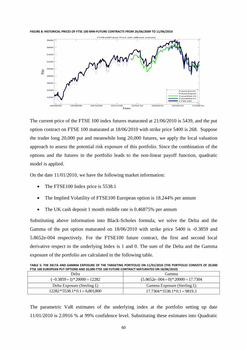
60

FIGURE 8: HISTORICAL PRICES OF FTSE 100 MIN-FUTURE CONTRACTS FROM 26/06/2009 TO 11/06/2010

The current price of the FTSE 100 index futures maturated at 21/06/2010 is 5439, and the put

option contract on FTSE 100 maturated at 18/06/2010 with strike price 5400 is 268. Suppose

the trader long 20,000 put and meanwhile long 20,000 futures, we apply the local valuation

approach to assess the potential risk exposure of this portfolio. Since the combination of the

options and the futures in the portfolio leads to the non-linear payoff function, quadratic

model is applied.

On the date 11/01/2010, we have the following market information:

The FTSE100 Index price is 5538.1

The Implied Volatility of FTSE100 European option is 18.244% per annum

The UK cash deposit 1 month middle rate is 0.46875% per annum

Substituting above information into Black-Scholes formula, we solve the Delta and the

Gamma of the put option maturated on 18/06/2010 with strike price 5400 is -0.3859 and

5.8652e-004 respectively. For the FTSE100 future contract, the first and second local

derivative respect to the underlying Index is 1 and 0. The sum of the Delta and the Gamma

exposure of the portfolio are calculated in the following table.

TABLE 5: THE DELTA AND GAMMA EXPOSURE OF THE TARGETING PORTFOLIO ON 11/01/2010 (THE PORTFOLIO CONSISTS OF 20,000 FTSE 100 EUROPEAN PUT OPTIONS AND 20,000 FTSE 100 FUTURE CONTRACT MATURATED ON 18/06/2010)

Delta Gamma

1228220000*)13859.0( 7304.1720000*)0004-5.8652e(

Delta Exposure (Sterling £) Gamma Exposure (Sterling £)

800,801,61.0*1.5538*12282 3.98191.0*1.5538*7304.17

The parametric VaR estimates of the underlying index at the portfolio setting up date

11/01/2010 is 2.0916 % at 99% confidence level. Substituting these estimates into Quadratic

26/06/09 15/08/09 04/10/09 23/11/09 12/01/10 03/03/10 22/04/10 11/06/10

4200

4400

4600

4800

5000

5200

5400

5600

5800

Date

Price

FTSE100Future Price with different maturity

FutureJun10

FutureSep10

FutureDec10

FutureMar11

FTSE100

61

Model, the daily portfolio’s VaR estimate at 99% confidence level is equal to 130,325GBP.

Suppose the trade holds the portfolio for the next 10 days, the 10-day VaR is approximately

412,120GBP using time square root rule.

For back-testing purpose, we check the actual index value on the date 12/01/2010 (10 days

after), which turn out to be 5260.3. The corresponding future price dropped to 5175. The total

realized loss of the targeting portfolio is calculated in the following table:

TABLE 6: THE TOTAL REALIZED LOSS OF THE TARGETING PORTFOLIO ON 12/01/2010

Actual loss from longing Index Future P-528,000GB0.1*5439)-(5175*20000

Actual profit from put options GBP800,225268*200 -0.1*5260.3) - (5400*20000

Total realized Loss GBP200,30222,580,0-52,800,0

The realized loss is below the estimated VaR level, supporting the result from the quadratic

model. It could be found that when the Gamma is positive, the quadratic approximation will

decrease the delta-Normal VaR, since the second term in the equation (2.29) will decrease the

overall value, and vice verse. This is intuitively true because the positive Gamma corresponds

to the net long position in the options. The holder of option always has the limited downside

risk.

However, when looking back the result in table 5, we find that the value of the delta exposure

is much greater than the gamma exposure, implying that the overall market risk of the

portfolio is dominated by the delta risk. More explicitly, if we calculate the value of the first

term and second term in the equation (2.29) separately, we have:

Delta risk = = 134,678

Gamma risk =

= 4354

Therefore even we only consider the delta risk (linear risk exposure), the VaR estimate will

fully enough to capture the actual loss. The delta risk reliance property in the local valuation

approach, on the other hand, imposes a potential danger to the risk manger. That is, if the

target portfolio has low delta exposure, local valuation approach which put too much weight

to the delta exposure will tends to underestimates the true risk.

Portfolio 2: Short Straddle

The best way to examine the potential weakness mentioned above is to implement this

approach to a target portfolio which is close to delta neutral at the measurement date. Since

the delta represents the linear risk exposure, a delta neutral portfolio could be constructed by

simultaneously longing and shorting the assets with similar level of delta exposure. For

62

instance, by selling a both puts and call options written on the same underlying asset, we can

construct an option portfolio (straddle) which theoretically has no delta risk exposure at the

initial setting up date. Although the portfolio has no delta risk exposure, it is actually fairly

risky because either up movement or down movement of the underlying price will lead to a

potentially large loss.

We use the same dataset in the section 3.3 to perform the risk assessment. Suppose a trader is

now at time 16/02/2010 when the market implied volatility is around 20% per annum. Given

that the volatility has stayed at this level for the last few months, he predicts that the market

will continue to be stable for the next one month and thereby implement a strategy by

simultaneously selling 20,000 calls and puts on FTSE 100 index (short straddle). If the index

value maintain at current level, this short straddle will be profitable. On the other hand, if the

prediction is wrong and the market becomes more volatile, either the moving upwards or

downwards of the underlying index will lead to a potential unlimited loss.

We apply the Quadratic model in above section to measure the risk of this portfolio. On the

date 16/02/2010, the value of FTSE 100 Index is 5244.1. The market price for the option

contract on FTSE 100 maturated at 09/03/10 is illustrated in the table below:

TABLE 7: MARKET PRICE OF FTSE 100 EUROPEAN OPTIONS ON 09/03/10

Strike 4800 4900 5000 5100 5200 5300 5400 5500

Call 439.5 351.5 268.5 193.5 129 78.5 43 21.5

Put 24 35.5 52.5 77.5 113 162.5 227 305

The trader predict the market index will maintain around current level(5244.1) for the next

month and implement short straddle strategy by simultaneously writing 20,000 calls and puts

(200 contracts of the each option), with the strike price equal to 5300. The total premium

received by this strategy is 48,200 and the strategy is delta-neutral at the initial portfolio

setting-up date.

Using the market implied volatility at 16/02/2010 (which is 20.863% per annum) as the daily

volatility of FTSE 100, the parametric VaR estimate of the underlying index for one month is

therefore equal to:

where is the standard quantile at given significant level

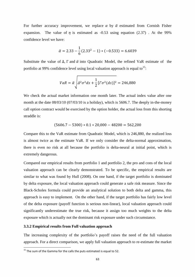
63

For further accuracy improvement, we replace by estimated from Cornish Fisher

expansion. The value of is estimated as -0.53 using equation (2.37) . At the 99%

confidence level we have:

Substitute the value of , and into Quadratic Model, the refined VaR estimate of the

portfolio at 99% confidence level using local valuation approach is equal to15

:

We check the actual market information one month later. The actual index value after one

month at the date 08/03/10 (07/03/10 is a holiday), which is 5606.7. The deeply in-the-money

call option contract would be exercised by the option holder, the actual loss from this shorting

straddle is:

Compare this to the VaR estimate from Quadratic Model, which is 246,880, the realized loss

is almost twice as the estimate VaR. If we only consider the delta-normal approximation,

there is even no risk at all because the portfolio is delta-neural at initial point, which is

extremely dangerous.

Compared our empirical results from portfolio 1 and portfolio 2, the pro and cons of the local

valuation approach can be clearly demonstrated. To be specific, the empirical results are

similar to what was found by Hull (2008). On one hand, if the target portfolio is dominated

by delta exposure, the local valuation approach could generate a safe risk measure. Since the

Black-Scholes formula could provide an analytical solution to both delta and gamma, this

approach is easy to implement. On the other hand, if the target portfolio has fairly low level

of the delta exposure (payoff function is serious non-linear), local valuation approach could

significantly underestimate the true risk, because it assign too much weights to the delta

exposure which is actually not the dominant risk exposure under such circumstance.

3.3.2 Empirical results from Full valuation approach

The increasing complexity of the portfolio’s payoff raises the need of the full valuation

approach. For a direct comparison, we apply full valuation approach to re-estimate the market

15

The sum of the Gamma for the calls the puts estimated is equal to 52.

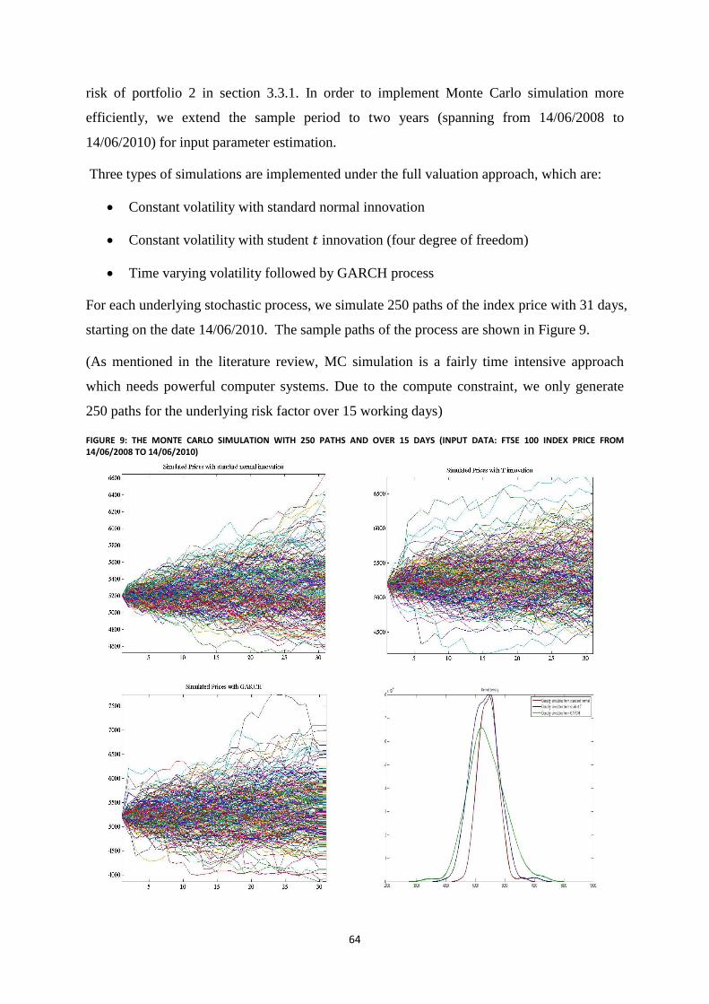
64

risk of portfolio 2 in section 3.3.1. In order to implement Monte Carlo simulation more

efficiently, we extend the sample period to two years (spanning from 14/06/2008 to

14/06/2010) for input parameter estimation.

Three types of simulations are implemented under the full valuation approach, which are:

Constant volatility with standard normal innovation

Constant volatility with student innovation (four degree of freedom)

Time varying volatility followed by GARCH process

For each underlying stochastic process, we simulate 250 paths of the index price with 31 days,

starting on the date 14/06/2010. The sample paths of the process are shown in Figure 9.

(As mentioned in the literature review, MC simulation is a fairly time intensive approach

which needs powerful computer systems. Due to the compute constraint, we only generate

250 paths for the underlying risk factor over 15 working days)

FIGURE 9: THE MONTE CARLO SIMULATION WITH 250 PATHS AND OVER 15 DAYS (INPUT DATA: FTSE 100 INDEX PRICE FROM 14/06/2008 TO 14/06/2010)

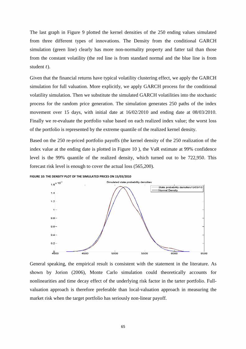
65

The last graph in Figure 9 plotted the kernel densities of the 250 ending values simulated

from three different types of innovations. The Density from the conditional GARCH

simulation (green line) clearly has more non-normality property and fatter tail than those

from the constant volatility (the red line is from standard normal and the blue line is from

student ).

Given that the financial returns have typical volatility clustering effect, we apply the GARCH

simulation for full valuation. More explicitly, we apply GARCH process for the conditional

volatility simulation. Then we substitute the simulated GARCH volatilities into the stochastic

process for the random price generation. The simulation generates 250 paths of the index

movement over 15 days, with initial date at 16/02/2010 and ending date at 08/03/2010.

Finally we re-evaluate the portfolio value based on each realized index value; the worst loss

of the portfolio is represented by the extreme quantile of the realized kernel density.

Based on the 250 re-priced portfolio payoffs (the kernel density of the 250 realization of the

index value at the ending date is plotted in Figure 10 ), the VaR estimate at 99% confidence

level is the 99% quantile of the realized density, which turned out to be 722,950. This

forecast risk level is enough to cover the actual loss (565,200).

FIGURE 10: THE DENSITY PLOT OF THE SIMULATED PRICES ON 15/03/2010

General speaking, the empirical result is consistent with the statement in the literature. As

shown by Jorion (2006), Monte Carlo simulation could theoretically accounts for

nonlinearities and time decay effect of the underlying risk factor in the tarter portfolio. Full-

valuation approach is therefore preferable than local-valuation approach in measuring the

market risk when the target portfolio has seriously non-linear payoff.

66

On the other hand, when comparing the hypothetical portfolio 1 and portfolio 2 constructed

in this research, we found that these two portfolios actually have same degree of non-linearity,

because their non-linearity are driven by the same risk source which is the equity option. The

key difference between their payoff functions, however, is that the portfolio 1’s payoff is

monotonic while the portfolio 2’s payoff is non-monotonic. This fact indicates that rather

than non-linearity, whether the payoff is monotonic is the critical consideration to select the

appropriate risk exposure modeling technique.

Local valuation approach with quadratic approximation can be enough for the portfolio with

fairly non-linear payoff, as long as it is monotonic. However, when the portfolio has

seriously non-monotonous payoff, the overall delta exposure tend to be cancel out due to the

hedge effect. Local valuation approach therefore leads to the underestimation of the true

market risk even Cornish-fisher expansion used as a complement. Full valuation approach by

Monte Carlo simulation is recommended under such situation.

3.4 Risk measurement of the foreign currency

3.4.1 Findings from the local valuation approach

Having studying the equity risk factor, we now turn to the model application of exchange rate

risk. Exposure to the foreign exchange risk is a natural result of the globalization of the

financial institutions. To be specific, the exchange risk influences the global investment in

two ways:

Exchange rate risk increase the uncertainty of translating the value of the foreign asset

back in to the domestic currency.

Exchange rate changes will influence the return on the foreign asset due to their

correlation. (e.g.: appreciation of the foreign currency will have a negative effect on

the foreign exporter which decrease the return on their asset)

Unexpected volatility of the exchange rate risk can generate substantial loss to the firm,

which in turn threaten their profitability or even survival. In practice, firms engaged in the

international business could use currency forward or future contract to hedge the exchange

rate risk. For instance, if the firm is expecting to receive certain amount of the foreign

currency payment in the future, it can simply lock the exchange rate by entering into a short

position in corresponding foreign currency forwards.

67

From the view of the financial institutions, they have even more exposure to the exchange

rate risk than the firms due to their more frequent foreign currency trading activities. These

activities include:

Act as the counterparty to the hedgers (firms) for the risk transfer

Offset the exposure in a given currency for hedging purposes

Speculate on the foreign currencies in search of potential profit

Because of the significant positions in the foreign currency contracts taken by the financial

institutions, they must measure and price this risk even more carefully and accurately than the

Non-financial enterprises.

Hull (2008) shows that the pricing formula of a foreign currency forward at time is

expressed as:

(3.6)

where:

is the sport price of the foreign currency at time

is the interest rate on the foreign currency

is the forward price of the contract

is the time to maturity

Jorion (2006) shows that under the local valuation approach, the market risk of the foreign

currency forward can be separated into three parts: the risk from the spot exchange rate, the

risk from the domestic zero rate and the risk from foreign zero rate. Review the Local-

valuation approach we implement in the section 3.3, the approach is actually a special case of

Taylor expansion. More generally, assuming the value of a derivative depends on the

underlying price, interest rate, yield from the underlying, volatility of the underlying and time,

Taylor expansion shows that (ignore higher order )16

:

(3.7)

where , , and are the partial derivatives respect to , and

16

Black-Scholes formula provides a closed-form solution for each partial derivative.

68

Applying Taylor expansion (3.11) to equation (3.10) and ignore the time subscript t we have:

(3.8)

We can further re-write the discount factor as the price of zero-bond, whose principal is one

unit of the currency, which is:

(3.9)

Where and are the price of zero-bond with domestic and foreign currency respectively

Substituting equation (3.9) into equation (3.8) we have:

(3.10)

Equation (3.10) is nothing more than a three factor model, which states that buying one

foreign currency forward can be decomposed into three cash flows:

Longing units’ spot foreign currency

longing units’ foreign zero bond and

Shorting units’ domestic zero bond

This decomposing not only provides an analytical approach for the foreign currency risk

modeling, but also gives us valuable implication for the foreign currency risk management.

Theoretically, the value of forward contract should be zero on the contract sign up date. The

risk decomposing from equation (3.10) indicates that if the trader is evaluate the market risk

of the currency forward at the contract signing up date, the quantities of longing foreign zero

bonds should be equal to the quantifies of shorting domestic zero bonds17

. In this case, the

long-short positions should diversity out large part of the interest rate risk if there is a high

correlation between the zero rates in the two countries.

3.4.2 Empirical analysis

To check the inference, this section implement the Jorion’ decomposing (3.10) to estimate the

market risk of a hypothetical foreign currency forward position. Consider a 1 year currency

forward contract of the Sterling against the US dollar, Figure 11 displays the movements of

17

will be equal to if setting equal to zero in equation (3.6)

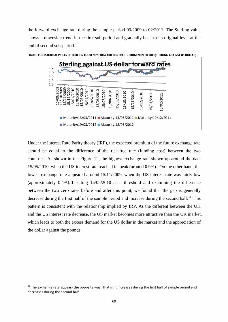
69

the forward exchange rate during the sample period 09/2009 to 02/2011. The Sterling value

shows a downside trend in the first sub-period and gradually back to its original level at the

end of second sub-period.

FIGURE 11: HISTORICAL PRICES OF FOREIGN CURRENCY FORWARD CONTRACTS FROM 2009 TO 2011(STERLING AGAINST US DOLLAR)

Under the Interest Rate Parity theory (IRP), the expected premium of the future exchange rate

should be equal to the difference of the risk-free rate (funding cost) between the two

countries. As shown in the Figure 12, the highest exchange rate shown up around the date

15/05/2010, when the US interest rate reached its peak (around 0.9%). On the other hand, the

lowest exchange rate appeared around 15/11/2009, when the US interest rate was fairly low

(approximately 0.4%).If setting 15/05/2010 as a threshold and examining the difference

between the two zero rates before and after this point, we found that the gap is generally

decrease during the first half of the sample period and increase during the second half.18

This

pattern is consistent with the relationship implied by IRP. As the different between the UK

and the US interest rate decrease, the US market becomes more attractive than the UK market,

which leads to both the excess demand for the US dollar in the market and the appreciation of

the dollar against the pounds.

18

The exchange rate appears the opposite way. That is, it increases during the first half of sample period and decreases during the second half

1.3 1.4 1.5 1.6 1.7

15

/09

/20

09

1

5/1

0/2

00

9

15

/11

/20

09

1

5/1

2/2

00

9

15

/01

/20

10

1

5/0

2/2

01

0

15

/03

/20

10

15

/04

/20

10

15

/05

/20

10

15

/06

/20

10

15

/07

/20

10

15

/08

/20

10

15

/09

/20

10

15

/10

/20

10

15

/11

/20

10

15

/12

/20

10

15

/01

/20

11

15

/02

/20

11

Sterling against US dollar forward rates

Maturity:13/03/2011 Maturity:13/06/2011 Maturity:19/12/2011

Maturity:19/03/2012 Maturity:18/06/2012

70

FIGURE 12: ONE YEAR ZERO RATE CURVE IN THE UK AND THE US MARKET FROM 2009 TO 2010

Statistically, we construct a EWMA-covariance matrix for the spot exchange rate and 1

year spot rate in both domestic (UK) and foreign market (US)( and ) based on the 2 years

sample data from 2009 to 2010. The formula is given by Jose, Lopez and Walter (2001):

(3.11)

Where is the sample size and , are the spot rate of UK and US respectively

(The decay factor is setting to 0.984 for the daily date, which was adopted by the

Riskmetrics)

As shown in Table 8, the spot exchange rate has a estimated daily volatility of 0.7024%,

which is considerable greater than those for the US and the UK zero rate, (0.0358% and

0.0370% respectively), indicating that the risk of this currency forward is mainly driven by

the spot exchange rate. On the other hand, the relatively low positive correlation (0.1817)

between the US zero rate and the spot exchange rate and the low negative correlation (-

0.1563) between the UK zero rate and the spot exchange rate both indicated that there exists

certain diversification effect among these three risk factors, which will decrease the overall

risk of the currency forward. Finally, the high positive correlation between the US and the

UK zero rate indicate that the interest rate risk from these two countries could largely

diversify out from the long-short positions indicated by equation (3.10).

0.5

0.55

0.6

0.65

0.7

0.75

15

/09

/20

09

15

/11

/20

09

15

/01

/20

10

15

/03

/20

10

15

/05

/20

10

15

/07

/20

10

15

/09

/20

10

15

/11

/20

10

15

/01

/20

11

US/UK spot Exchange Rate

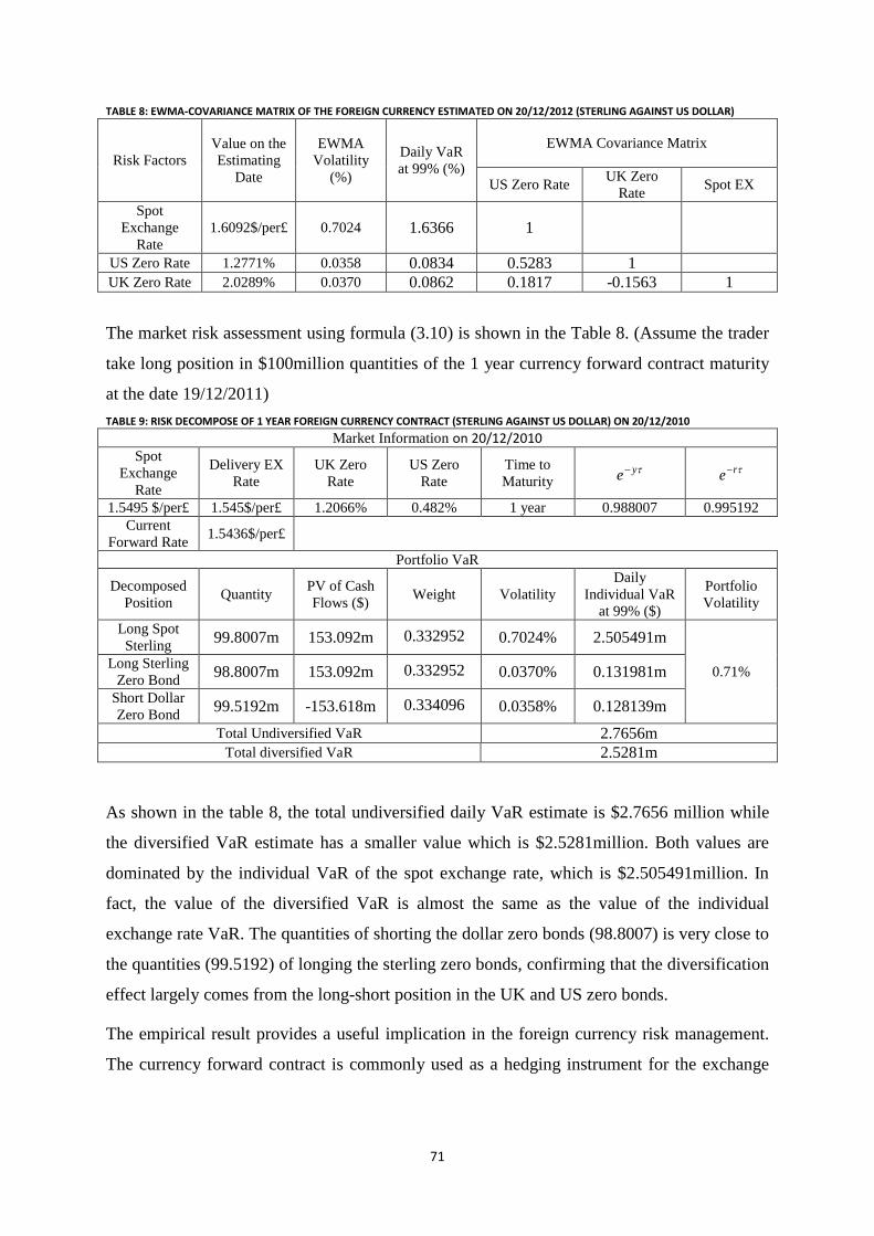
71

TABLE 8: EWMA-COVARIANCE MATRIX OF THE FOREIGN CURRENCY ESTIMATED ON 20/12/2012 (STERLING AGAINST US DOLLAR)

Risk Factors

Value on the

Estimating

Date

EWMA

Volatility

(%)

Daily VaR

at 99% (%)

EWMA Covariance Matrix

US Zero Rate UK Zero

Rate Spot EX

Spot

Exchange

Rate

1.6092$/per£ 0.7024 1.6366 1

US Zero Rate 1.2771% 0.0358 0.0834 0.5283 1

UK Zero Rate 2.0289% 0.0370 0.0862 0.1817 -0.1563 1

The market risk assessment using formula (3.10) is shown in the Table 8. (Assume the trader

take long position in $100million quantities of the 1 year currency forward contract maturity

at the date 19/12/2011)

TABLE 9: RISK DECOMPOSE OF 1 YEAR FOREIGN CURRENCY CONTRACT (STERLING AGAINST US DOLLAR) ON 20/12/2010

Market Information on 20/12/2010

Spot

Exchange

Rate

Delivery EX

Rate

UK Zero

Rate

US Zero

Rate

Time to

Maturity ye

re

1.5495 $/per£ 1.545$/per£ 1.2066% 0.482% 1 year 0.988007 0.995192

Current

Forward Rate 1.5436$/per£

Portfolio VaR

Decomposed

Position Quantity

PV of Cash

Flows ($) Weight Volatility

Daily

Individual VaR

at 99% ($)

Portfolio

Volatility

Long Spot

Sterling 99.8007m 153.092m 0.332952 0.7024% 2.505491m

0.71% Long Sterling

Zero Bond 98.8007m 153.092m 0.332952 0.0370% 0.131981m

Short Dollar

Zero Bond 99.5192m -153.618m 0.334096 0.0358% 0.128139m

Total Undiversified VaR 2.7656m

Total diversified VaR 2.5281m

As shown in the table 8, the total undiversified daily VaR estimate is $2.7656 million while

the diversified VaR estimate has a smaller value which is $2.5281million. Both values are

dominated by the individual VaR of the spot exchange rate, which is $2.505491million. In

fact, the value of the diversified VaR is almost the same as the value of the individual

exchange rate VaR. The quantities of shorting the dollar zero bonds (98.8007) is very close to

the quantities (99.5192) of longing the sterling zero bonds, confirming that the diversification

effect largely comes from the long-short position in the UK and US zero bonds.

The empirical result provides a useful implication in the foreign currency risk management.

The currency forward contract is commonly used as a hedging instrument for the exchange

72

rate risk in practice, if the currency future contains certain level of interest rate risk, the

hedging effectiveness will be affected.

The implication is that if the trader is evaluate the market risk at forward contract signing up

date (in this case), the quantities of longing the zero bonds in the foreign country should be

theoretically equal to the quantities of shorting the zero bonds in the domestic country. Under

such circumstance, the long-short positions will diversity out the large part of the interest rate

risk given that there is a high correlation between the two zero rates. This is exactly the true

in our example, where the valuation date is just one day after the contract signing up date and

the quantities of shorting the dollar zero bonds (98.8007) is very close to the quantifies

(99.5192) of longing the sterling zero bonds.

On the other hand, if the risk valuation date is far from the contract initializing date, the

interest rate risk should be considered additionally in the currency risk management (

will possibly derivate from ), because this risk could not be fully hedged by the unequal

long-short position in two zero bonds. From the perspective of the risk managers, it is

therefore necessary to notice that as the time deviated from the initial hedging date, the

forward contract will expose to certain degree of interest rate risk which might not be ignored.

3.5 Risk measurement of the bond portfolio

The last market risk we considered in this research is the interest rate risk. The risk factor is

particularly been concerned in the fixed-income investment. Risk measurement of the fixed-

income portfolio should put more emphasis on the risk mapping techniques than the equity

portfolio. Because unlike the equity portfolio whose risk could be summarized by single risk

factor (market index), the risk profile of the bond portfolio is captured by several risk factors,

including duration, key rate duration (yield twist), present value distribution of cash flows

(PVD) and credit spread. When the bond has embedded option, its optionality (Delta, Gamma

and implied volatilities) should be considered as well.

3.5.1 Risk profile analysis in the UK bond market

To perform an empirical analysis of the interest rate risk in the UK market, we collected the

historical data of the UK treasury strips with maturities spanning from 1 to 30 years, as

shown in the Table 10. Since we does not take account the credit risk in this research, the

bond selected are all sovereign bonds which has fairly low level of default risk.

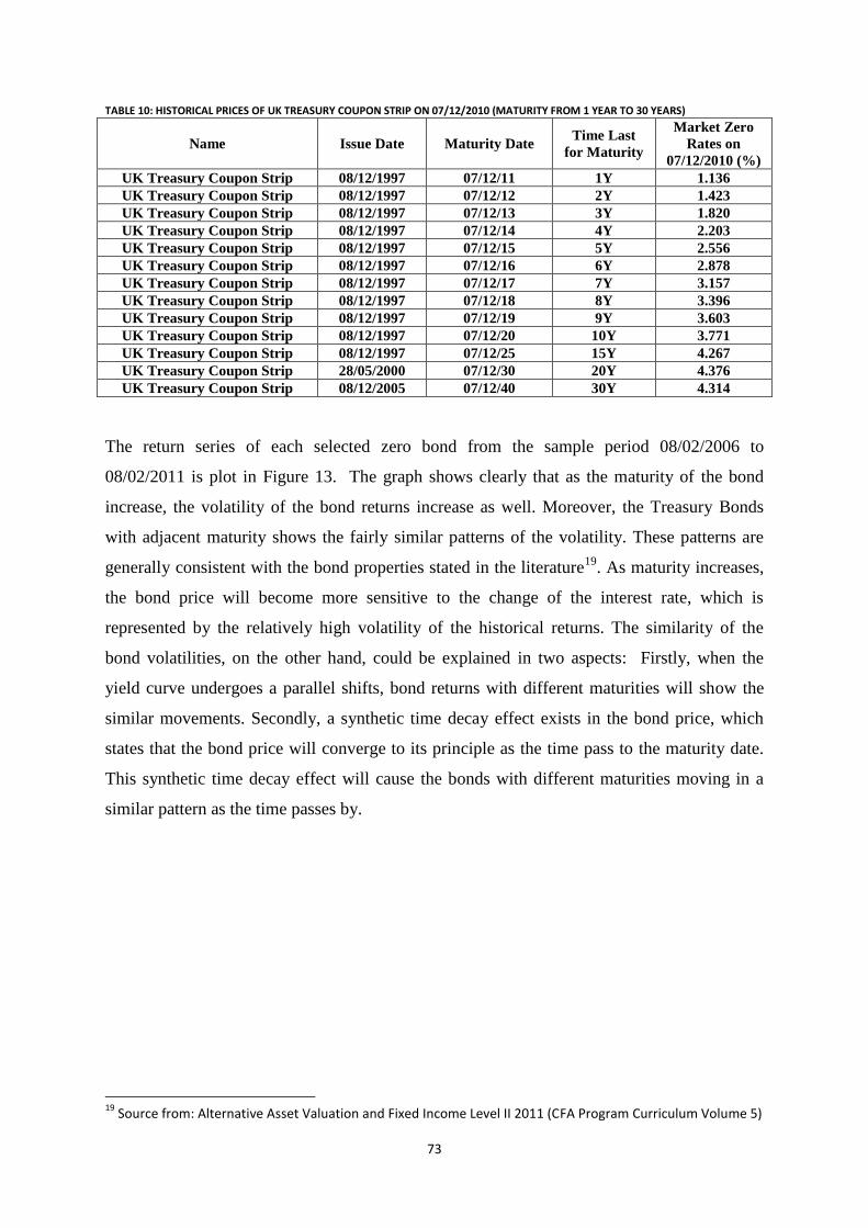
73

TABLE 10: HISTORICAL PRICES OF UK TREASURY COUPON STRIP ON 07/12/2010 (MATURITY FROM 1 YEAR TO 30 YEARS)

Name Issue Date Maturity Date Time Last

for Maturity

Market Zero

Rates on

07/12/2010 (%)

UK Treasury Coupon Strip 08/12/1997 07/12/11 1Y 1.136

UK Treasury Coupon Strip 08/12/1997 07/12/12 2Y 1.423

UK Treasury Coupon Strip 08/12/1997 07/12/13 3Y 1.820 UK Treasury Coupon Strip 08/12/1997 07/12/14 4Y 2.203 UK Treasury Coupon Strip 08/12/1997 07/12/15 5Y 2.556 UK Treasury Coupon Strip 08/12/1997 07/12/16 6Y 2.878 UK Treasury Coupon Strip 08/12/1997 07/12/17 7Y 3.157 UK Treasury Coupon Strip 08/12/1997 07/12/18 8Y 3.396

UK Treasury Coupon Strip 08/12/1997 07/12/19 9Y 3.603

UK Treasury Coupon Strip 08/12/1997 07/12/20 10Y 3.771

UK Treasury Coupon Strip 08/12/1997 07/12/25 15Y 4.267

UK Treasury Coupon Strip 28/05/2000 07/12/30 20Y 4.376

UK Treasury Coupon Strip 08/12/2005 07/12/40 30Y 4.314

The return series of each selected zero bond from the sample period 08/02/2006 to

08/02/2011 is plot in Figure 13. The graph shows clearly that as the maturity of the bond

increase, the volatility of the bond returns increase as well. Moreover, the Treasury Bonds

with adjacent maturity shows the fairly similar patterns of the volatility. These patterns are

generally consistent with the bond properties stated in the literature19

. As maturity increases,

the bond price will become more sensitive to the change of the interest rate, which is

represented by the relatively high volatility of the historical returns. The similarity of the

bond volatilities, on the other hand, could be explained in two aspects: Firstly, when the

yield curve undergoes a parallel shifts, bond returns with different maturities will show the

similar movements. Secondly, a synthetic time decay effect exists in the bond price, which

states that the bond price will converge to its principle as the time pass to the maturity date.

This synthetic time decay effect will cause the bonds with different maturities moving in a

similar pattern as the time passes by.

19

Source from: Alternative Asset Valuation and Fixed Income Level II 2011 (CFA Program Curriculum Volume 5)

74

FIGURE 13: THE HISTORICAL RETURN SERIES OF UK TREASURY COUPON STRIPS (FROM 2006 TO 2011)

1. Risk mapping using duration model

Quantitatively, we apply EWMA model to estimate the daily volatility of each selected zero

bond (see Table 11). Individual Bond returns VaR is calculated as the product of the

estimated volatility and the standard normal quantile ( ). In the last column of

Table 11, we implement the duration model to transfer the individual bond returns VaR to the

Yield VaR, which is given by Jorion (2006):

(3.12)

where is the modified duration and is the bond price

As pointed out by Jorion, the risk mapping using duration model (3.12) allows the user to

examine whether the yield curve undertakes a parallel shift during the sample period. If the

yield curve occurs a strictly parallel shift, the transferred yield VaR from equation (3.12)

should be constant across all maturities and under such situation, the duration should be a

valid and appropriate underlying risk factor for the market risk measure of the bond portfolio.

Focusing on the Table 11, we found that although the estimated yield VaR in the last column

appears not constant over different maturities, they are fairly stable as opposed to the high

fluctuated Return VaR, except that the zero bonds with one year and two year maturity have a

75

relatively lower yield VaR. The result is an evidence to support that the yield curve

undertakes a parallel shift during the sample period in the UK market.

However, as we pointed out at the end of the section 3.5.1, there exists one critical problem

of applying duration measurement, which is the ignorance of the synthetic time decay effect

in the historical bond returns. When we re-examine the duration model (3.12), we found that

this model completely ignore this synthetic time decay effect as well. More explicitly, the

relationship between the bond returns and the yield change in equation (3.12) should only be

hold theoretically when the time is fixed at the certain time point. However, since the

historical bond price series are observed at the different time date, the synthetic time decay

effect will lead to the fact that the bond price becomes less sensible to the interest rate change

and gradually converge to its principle. Therefore fitting Jorion’s duration model into the

historical bond price series will have a mislead effect of distinguishing whether the stability

of the yield VaR is due to the external parallel shift or simply the synthetic time decay effect.

TABLE 11: UK TREASURY COUPON STRIPS VAR ESTIMATE USING DURATION MODEL ON 07/12/2010 (INPUT DATA: HISTORICAL PRICES FROM 10/11/2006 TO 06/12/2010)

Maturity Year Return Volatility

(%)

Market Yield

(%)

Modified

Duration

Returns

VaR (%)

Yield

VaR (%)

1 0.029 1.136 0.988768 0.065 0.066

2 0.063 1.423 1.971939 0.148 0.075

3 0.131 1.820 2.946376 0.306 0.104

4 0.190 2.203 3.913779 0.443 0.113

5 0.247 2.556 4.875385 0.576 0.118

6 0.303 2.878 5.832151 0.707 0.121

7 0.351 3.157 6.785773 0.818 0.121

8 0.403 3.396 7.737243 0.939 0.121

9 0.457 3.603 8.687007 1.065 0.123

10 0.485 3.771 9.636604 1.130 0.118

15 0.678 4.267 14.38614 1.580 0.110

20 0.870 4.376 19.16149 2.027 0.106

30 1.244 4.314 28.75932 2.899 0.101

2. Risk mapping using Principal Component Analysis (PCA)

To check the inference from the duration model that the yield curve undergone a roughly

parallel shift in the UK market, we collect the historical data of the UK zero rate over the

same sample period. Figure 14 plot the UK zero yield surface with maturity from 1 year to 30

years, and 5 years sample period spanning from 08/02/2006 to 08/02/2011. It can be seen

clearly from the graph that the term structure of the yield curve undergone certain degree of

non-parallel shifts during the sample period, which is inconsistent with the results from the

duration model. This supports our statement in the above section that applying duration

76

model will possibly underestimate the true interest rate risk raised from the actual

asynchronous movement of the yield curve.

FIGURE 14: THE UK ZERO RATE YIELD SURFACE MATURITY FROM 1 YEAR TO 30 YEARS (SAMPLE PERIOD SPANNING FROM 2006 TO 2011)

This section implements a more comprehensive risk mapping technique, which is Principal

component analysis. Table 11 shows the correlation matrix of the changes of the UK zero

rates during the sample period. The correlations are considerable high and positive for the

adjacent maturities and tend to decrease with the spread between maturities. The lowest

correlation arrives at the maturity between 1 year and 30 year, which is 0.315. The positive

correlations across all maturities, on the other hand, indicate that there are some common

factors which dominate the changes of the zero rates of the different maturities in the UK

financial market.

TABLE 12: THE CORRELATION MATRIX OF THE UK ZERO YIELDS (ESTIMATED USING SAMPLE DATA FROM 2006 TO 2011)

Year 1 2 3 4 5 6 7 8 9 10 15 20 30

1 1.000

2 0.892 1.000

3 0.792 0.970 1.000

4 0.736 0.935 0.988 1.000

5 0.690 0.900 0.967 0.992 1.000

6 0.646 0.863 0.940 0.975 0.993 1.000

7 0.603 0.821 0.903 0.947 0.976 0.992 1.000

8 0.557 0.773 0.861 0.912 0.948 0.975 0.993 1.000

9 0.521 0.734 0.825 0.880 0.923 0.956 0.983 0.996 1.000

10 0.494 0.703 0.795 0.854 0.900 0.938 0.971 0.989 0.997 1.000

15 0.443 0.640 0.733 0.796 0.848 0.894 0.935 0.961 0.975 0.984 1.000

20 0.404 0.593 0.686 0.750 0.803 0.851 0.895 0.924 0.941 0.953 0.985 1.000

30 0.315 0.487 0.576 0.635 0.684 0.732 0.777 0.807 0.827 0.842 0.893 0.941 1.000

Applying PCA (Table 13), the empirical result shows that there are three Principal

Components which could explain approximately 99% of the overall variation of the full

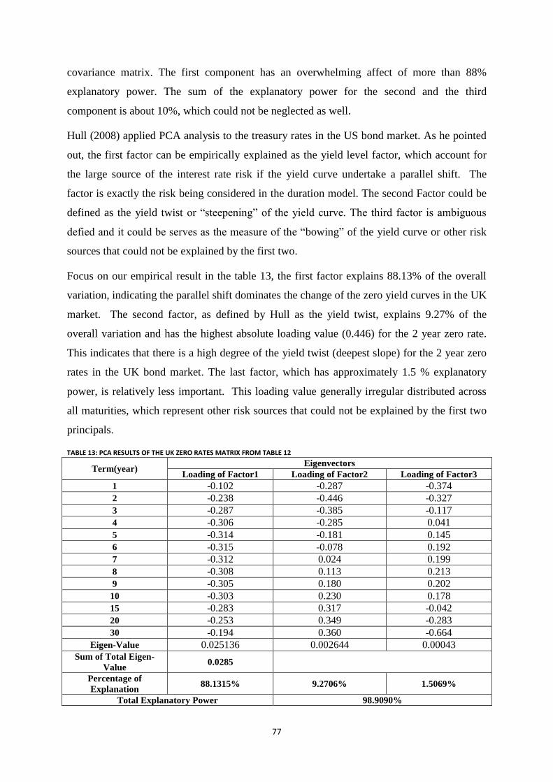
77

covariance matrix. The first component has an overwhelming affect of more than 88%

explanatory power. The sum of the explanatory power for the second and the third

component is about 10%, which could not be neglected as well.

Hull (2008) applied PCA analysis to the treasury rates in the US bond market. As he pointed

out, the first factor can be empirically explained as the yield level factor, which account for

the large source of the interest rate risk if the yield curve undertake a parallel shift. The

factor is exactly the risk being considered in the duration model. The second Factor could be

defined as the yield twist or “steepening” of the yield curve. The third factor is ambiguous

defied and it could be serves as the measure of the “bowing” of the yield curve or other risk

sources that could not be explained by the first two.

Focus on our empirical result in the table 13, the first factor explains 88.13% of the overall

variation, indicating the parallel shift dominates the change of the zero yield curves in the UK

market. The second factor, as defined by Hull as the yield twist, explains 9.27% of the

overall variation and has the highest absolute loading value (0.446) for the 2 year zero rate.

This indicates that there is a high degree of the yield twist (deepest slope) for the 2 year zero

rates in the UK bond market. The last factor, which has approximately 1.5 % explanatory

power, is relatively less important. This loading value generally irregular distributed across

all maturities, which represent other risk sources that could not be explained by the first two

principals.

TABLE 13: PCA RESULTS OF THE UK ZERO RATES MATRIX FROM TABLE 12

Term(year) Eigenvectors

Loading of Factor1 Loading of Factor2 Loading of Factor3

1 -0.102 -0.287 -0.374

2 -0.238 -0.446 -0.327

3 -0.287 -0.385 -0.117

4 -0.306 -0.285 0.041

5 -0.314 -0.181 0.145

6 -0.315 -0.078 0.192

7 -0.312 0.024 0.199

8 -0.308 0.113 0.213

9 -0.305 0.180 0.202

10 -0.303 0.230 0.178

15 -0.283 0.317 -0.042

20 -0.253 0.349 -0.283

30 -0.194 0.360 -0.664

Eigen-Value 0.025136 0.002644 0.00043 Sum of Total Eigen-

Value 0.0285

Percentage of

Explanation 88.1315% 9.2706% 1.5069%

Total Explanatory Power 98.9090%

78

PCA is more comprehensive compared to the duration model. Since it applied directly to the

yield rather than the bond historical returns, this approach also get rid of the synthetic time

decay effect. Mathematically, Jorion (2006) shows that the efficiency of PCA analysis could

be checked by constructing a new covariance matrix using the selected three PCAs and then

comparing it with the sample covariance matrix by the original zero yields series. The

equation is given by:

(3.13)

where is the Eigen-value of the PCA and is the corresponding loading vector.

In our example, the new covariance matrix is obtained by setting (See table 14 and

table 15). Comparing these two tables, the covariance matrix constructed by PCA give a

fairly good approximation of the original covariance matrix.

TABLE 14: THE COVARIANCE MATRIX CONSTRUCTED BY FULL SAMPLE RETURNS FROM 2006 TO 2011 0.00029

%

0.00035

%

0.00045

%

0.00040

%

0.00053

%

0.00065

%

0.00045

%

0.00061

%

0.00077

%

0.00095

%

0.00049

%

0.00068

%

0.00086

%

0.00108

%

0.00130

%

0.00054

%

0.00075

%

0.00096

%

0.00121

%

0.00144

%

0.00167

%

0.00058

%

0.00080

%

0.00103

%

0.00131

%

0.00157

%

0.00180

%

0.00202

%

0.00063

%

0.00087

%

0.00113

%

0.00143

%

0.00172

%

0.00199

%

0.00220

%

0.00247

%

0.00067

%

0.00093

%

0.00120

%

0.00153

%

0.00184

%

0.00213

%

0.00236

%

0.00266

%

0.00289

%

0.00071

%

0.00098

%

0.00127

%

0.00162

%

0.00197

%

0.00227

%

0.00251

%

0.00283

%

0.00306

%

0.00331

%

0.00081

%

0.00117

%

0.00155

%

0.00201

%

0.00247

%

0.00287

%

0.00318

%

0.00362

%

0.00393

%

0.00419

%

0.00620

%

0.00096

%

0.00139

%

0.00185

%

0.00241

%

0.00300

%

0.00349

%

0.00386

%

0.00441

%

0.00481

%

0.00513

%

0.00768

%

0.00995

%

0.00112

%

0.00166

%

0.00225

%

0.00294

%

0.00361

%

0.00424

%

0.00476

%

0.00537

%

0.00586

%

0.00628

%

0.00932

%

0.01232

%

0.01768

%

79

TABLE 15: THE COVARIANCE MATRIX CONSTRUCTED BY PCA 0.00022

%

0.00029

%

0.00038

%

0.00035

%

0.00047

%

0.00059

%

0.00043

%

0.00058

%

0.00073

%

0.00091

%

0.00049

%

0.00067

%

0.00085

%

0.00106

%

0.00126

%

0.00056

%

0.00076

%

0.00096

%

0.00121

%

0.00143

%

0.00164

%

0.00061

%

0.00083

%

0.00106

%

0.00132

%

0.00157

%

0.00180

%

0.00197

%

0.00066

%

0.00090

%

0.00116

%

0.00146

%

0.00174

%

0.00199

%

0.00219

%

0.00244

%

0.00070

%

0.00096

%

0.00124

%

0.00156

%

0.00187

%

0.00214

%

0.00235

%

0.00263

%

0.00283

%

0.00075

%

0.00103

%

0.00132

%

0.00167

%

0.00199

%

0.00228

%

0.00251

%

0.00280

%

0.00302

%

0.00322

%

0.00081

%

0.00116

%

0.00154

%

0.00200

%

0.00247

%

0.00288

%

0.00318

%

0.00363

%

0.00394

%

0.00421

%

0.00613

%

0.00093

%

0.00135

%

0.00182

%

0.00239

%

0.00298

%

0.00349

%

0.00387

%

0.00443

%

0.00483

%

0.00516

%

0.00773

%

0.00989

%

0.00112

%

0.00167

%

0.00225

%

0.00294

%

0.00361

%

0.00424

%

0.00476

%

0.00537

%

0.00585

%

0.00628

%

0.00931

%

0.01233

%

0.01768

%

3.5.2 Risk measurement integrating the mapping techniques

The above analysis of the interest rate risk profile in the UK bond market shows that the term

structure of the UK zero yields undergone a certain degree of nonparallel shift over the

sample period from 2006 to 2011. Applying the duration model could probably underestimate

the true interest rate risk. PCA analysis, on the other hand, provides a more comprehensive

consideration of the overall risk and it could incorporate the information from duration model

in its first factor loading.

To test the performance of these techniques, we construct some hypothetical bond portfolios

in the UK market and implement the risk measurement integrating the risk mapping

approaches. The bonds selected are all sovereign bonds or high investment-grade corporate

bonds with fairly low default risk.

1. Market risk measurement of the zero bond portfolio

The first bond portfolio constructed is a long-short bond portfolio consists of randomly

selected four UK Treasury Coupon Strips, which are:

1. Long £20m in 9- years’ Coupon Strip

2. Long £5m in 10-years’ Coupon Strip

3. Short £10m in 3-year’s Coupon Strip

4. Short £12m in 20-years’ Coupon Strip

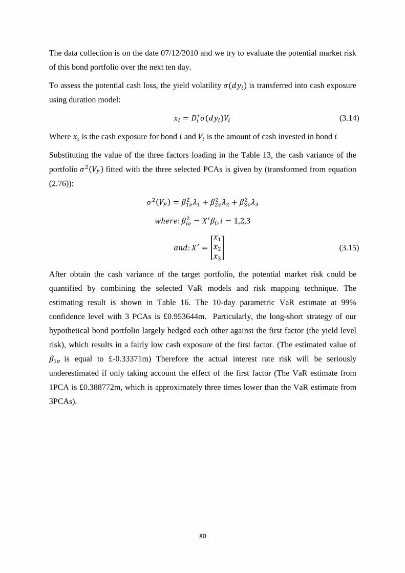
80

The data collection is on the date 07/12/2010 and we try to evaluate the potential market risk

of this bond portfolio over the next ten day.

To assess the potential cash loss, the yield volatility is transferred into cash exposure

using duration model:

(3.14)

Where is the cash exposure for bond and is the amount of cash invested in bond

Substituting the value of the three factors loading in the Table 13, the cash variance of the

portfolio fitted with the three selected PCAs is given by (transformed from equation

(2.76)):

(3.15)

After obtain the cash variance of the target portfolio, the potential market risk could be

quantified by combining the selected VaR models and risk mapping technique. The

estimating result is shown in Table 16. The 10-day parametric VaR estimate at 99%

confidence level with 3 PCAs is £0.953644m. Particularly, the long-short strategy of our

hypothetical bond portfolio largely hedged each other against the first factor (the yield level

risk), which results in a fairly low cash exposure of the first factor. (The estimated value of

is equal to £-0.33371m) Therefore the actual interest rate risk will be seriously

underestimated if only taking account the effect of the first factor (The VaR estimate from

1PCA is £0.388772m, which is approximately three times lower than the VaR estimate from

3PCAs).

81

TABLE 16: THE BOND PORTFOLIO VAR ESTIMATE ON 07/12/2010 USING DURATION AND PCA

Bonds

in

Portfolio

Current

Market

Zero

Yield (%)

Modified

Duration*iD

Yield

Volatility

idy

Market Value iV

(£million) Cash Exposures ix (£million)

3 year’s

Coupon

Strip

1.8203 2.946 4.99% -10 -1.47005

9 years’

Coupon

Strip

3.6019 8.687 4.95% +20 8.60013

10

years’

Coupon

Strip

3.7705 9.637 4.98% +5 2.399613

20

years’

Coupon

Strip

4.3764 19.161 4.46% -12 -10.255

Term Loading

of 1

Loading of

2

Loading

of 3

Eigen-Value Cash Exposure

(£million) Cash SD of

Portfolio(£m) 3y -0.287 -0.385 -0.117 1 0.025 v1 -0.33371

9y -0.305 0.180 0.202 2 0.0026 v2 5.328509 0.129425m

10y -0.303 0.230 0.178 3 0.00043 v3 -0.91308

20y -0.253 0.349 -0.283 10 day VaR at 99% 0.953644m

For back-testing purpose, we check the actual market prices of the bonds in the portfolio ten

day after on the date 21/12/2010, as shown in Table 17. The actual loss break the VaR

estimate from 1PCA, while the VaR estimate from 3PCAs (0.953644) is large enough to

incorporate the potential lose.

Given that the first factor is empirically defined as the yield level factor which covered in the

duration model, the empirical result shows that simply consideration of the yield level risk

could considerably underestimated the true interest rate risk in the UK market. This is

consistent with the empirical results found by Hull and Jorion. They both apply PCA analysis

on the US bond market and found that the one-factor PCA generates a fairly low VaR

compared to the two-factor PCAs. Furthermore, the yield level risk (parallel shift) will tend to

be canceled out by the long-short position in this hypothetical portfolio since we deliberately

selected a long-short strategy for the portfolio construction, which amplifies the yield

twisting risk. The one factor PCA (duration model) will become extremely dangerous

because it totally overlook the unparallel shift of the yield curve.

82

TABLE 17: THE REALIZED LOSS OF THE BOND PORTFOLIO ON 21/12/2010

Bonds in Portfolio Market Price

on 07/12/2010

Market Price

on 21/12/2010

Market Zero

Yields on

21/12/2010

(%)

Return (%) Portfolio

Loss(£m)

Short 3 year’s

Coupon Strip 95.94 95.5 2.0379 -0.459 0.045862m

Long 9 years’

Coupon Strip 72.5 72.32 3.6758 -0.248 -0.04966m

Long 10 years’

Coupon Strip 68.72 68.56 3.8171 -0.233 -0.01164m

Short 20 years’

Coupon Strip 39.54 40.91 4.2657 3.465 -0.41578m

Total Portfolio loss -0.43122m

Three PCAs VaR at 99% 0.953644m

One PCA VaR 0.33371m

2. Risk measurement of the coupon bond portfolio

The hypothetical bond portfolio constructed above contains all zero coupon bonds, which has

no reinvestment risk. For a more general consideration, we construct a coupon paying bond

portfolio. The market risk measurement of this type portfolio involves using vertex mapping

approach, which is a cash flow mapping approach minutely described by Henrard (2000).

The goal of the vertex mapping is to distribute the initial bond portfolio to certain adjoining

vertices that could serve as the best approximation of the overall interest rate risk. (In practice,

credit risk, liquidity risk and option-related risk should also be considered if necessarily).

Interest risk has two components, which are price risk and reinvestment risk20

. Since the

coupon bonds with large principal paid at maturities have low reinvestment risk, the selection

of the vertices should target on the cash flow risk around the principal payment date.

Define , as the duration of the two adjoined vertices whose duration is close to the

portfolio’s overall duration , the optimization procedure is expressed as:

(3.16)

Henrard pointed out that the duration mapping equation (3.16) is simple but may not be safe,

because it only focuses on the duration matching but does not guarantee the vertices will have

the same overall risk as the original portfolio. Hence, a more appropriate target should be

focus on calibrating the portfolio variance (both price risk and reinvestment risk), which is

expressed as:

20

Source: Alternative Asset Valuation and Fixed Income Level II 2011 (CFA Program Curriculum Volume 5)

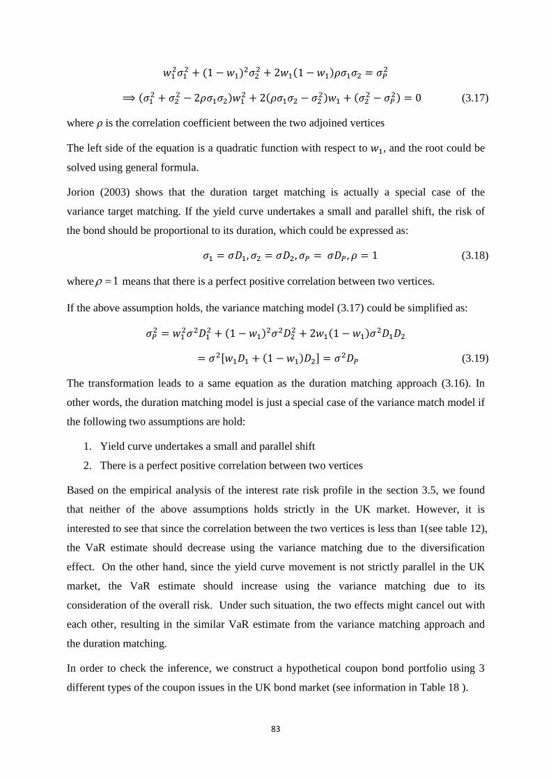
83

(3.17)

where is the correlation coefficient between the two adjoined vertices

The left side of the equation is a quadratic function with respect to , and the root could be

solved using general formula.

Jorion (2003) shows that the duration target matching is actually a special case of the

variance target matching. If the yield curve undertakes a small and parallel shift, the risk of

the bond should be proportional to its duration, which could be expressed as:

(3.18)

where 1 means that there is a perfect positive correlation between two vertices.

If the above assumption holds, the variance matching model (3.17) could be simplified as:

(3.19)

The transformation leads to a same equation as the duration matching approach (3.16). In

other words, the duration matching model is just a special case of the variance match model if

the following two assumptions are hold:

1. Yield curve undertakes a small and parallel shift

2. There is a perfect positive correlation between two vertices

Based on the empirical analysis of the interest rate risk profile in the section 3.5, we found

that neither of the above assumptions holds strictly in the UK market. However, it is

interested to see that since the correlation between the two vertices is less than 1(see table 12),

the VaR estimate should decrease using the variance matching due to the diversification

effect. On the other hand, since the yield curve movement is not strictly parallel in the UK

market, the VaR estimate should increase using the variance matching due to its

consideration of the overall risk. Under such situation, the two effects might cancel out with

each other, resulting in the similar VaR estimate from the variance matching approach and

the duration matching.

In order to check the inference, we construct a hypothetical coupon bond portfolio using 3

different types of the coupon issues in the UK bond market (see information in Table 18 ).

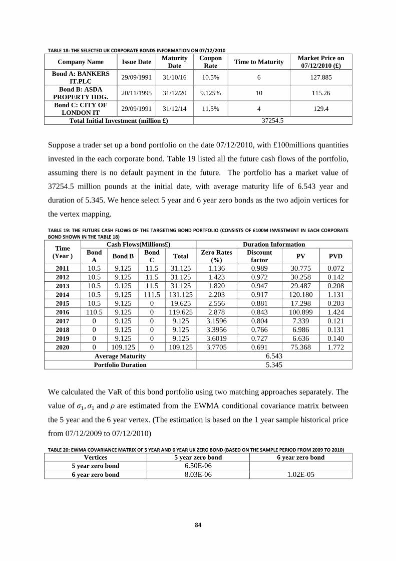
84

TABLE 18: THE SELECTED UK CORPORATE BONDS INFORMATION ON 07/12/2010

Company Name Issue Date Maturity

Date

Coupon

Rate Time to Maturity

Market Price on

07/12/2010 (£)

Bond A: BANKERS

IT.PLC 29/09/1991 31/10/16 10.5% 6 127.885

Bond B: ASDA

PROPERTY HDG. 20/11/1995 31/12/20 9.125% 10 115.26

Bond C: CITY OF

LONDON IT 29/09/1991 31/12/14 11.5% 4 129.4

Total Initial Investment (million £) 37254.5

Suppose a trader set up a bond portfolio on the date 07/12/2010, with £100millions quantities

invested in the each corporate bond. Table 19 listed all the future cash flows of the portfolio,

assuming there is no default payment in the future. The portfolio has a market value of

37254.5 million pounds at the initial date, with average maturity life of 6.543 year and

duration of 5.345. We hence select 5 year and 6 year zero bonds as the two adjoin vertices for

the vertex mapping.

TABLE 19: THE FUTURE CASH FLOWS OF THE TARGETING BOND PORTFOLIO (CONSISTS OF £100M INVESTMENT IN EACH CORPORATE BOND SHOWN IN THE TABLE 18)

Time

(Year )

Cash Flows(Millions£) Duration Information

Bond

A Bond B

Bond

C Total

Zero Rates

(%)

Discount

factor PV PVD

2011 10.5 9.125 11.5 31.125 1.136 0.989 30.775 0.072

2012 10.5 9.125 11.5 31.125 1.423 0.972 30.258 0.142

2013 10.5 9.125 11.5 31.125 1.820 0.947 29.487 0.208

2014 10.5 9.125 111.5 131.125 2.203 0.917 120.180 1.131

2015 10.5 9.125 0 19.625 2.556 0.881 17.298 0.203

2016 110.5 9.125 0 119.625 2.878 0.843 100.899 1.424

2017 0 9.125 0 9.125 3.1596 0.804 7.339 0.121

2018 0 9.125 0 9.125 3.3956 0.766 6.986 0.131

2019 0 9.125 0 9.125 3.6019 0.727 6.636 0.140

2020 0 109.125 0 109.125 3.7705 0.691 75.368 1.772

Average Maturity 6.543

Portfolio Duration 5.345

We calculated the VaR of this bond portfolio using two matching approaches separately. The

value of and are estimated from the EWMA conditional covariance matrix between

the 5 year and the 6 year vertex. (The estimation is based on the 1 year sample historical price

from 07/12/2009 to 07/12/2010)

TABLE 20: EWMA COVARIANCE MATRIX OF 5 YEAR AND 6 YEAR UK ZERO BOND (BASED ON THE SAMPLE PERIOD FROM 2009 TO 2010)

Vertices 5 year zero bond 6 year zero bond

5 year zero bond 6.50E-06

6 year zero bond 8.03E-06 1.02E-05

85

After obtained the EMWA covariance matrix, we estimate the portfolio variance by linear

interpolation of the variance of the 5 and 6-year zero bonds (portfolio duration is 5.345).The

corresponding VaR estimates using two vertex mapping approaches are illustrated in Table

21. As shown in the table, the VaR estimate from the variance target matching approach

(225.870) is less than that from the duration target matching approach (239.826). However,

this difference is fairly minor compared to the initial investment amount.

TABLE 21: THE BOND PORTFOLIO VAR ESTIMATE ON 07/12/2010 USING VERTEX MAPPING

Vertices Volatility (%) Individual VaR

(99%) Duration

Matching

Variance

Matching

5 year zero bond 0.255 0.594

0.986

1w 0.655 1w 0.614

6 year zero bond 0.319 0.744 2w 0.345 2w 0.386

Portfolio 0.279 Cash Weight Cash Weight

Market Value of Bond Portfolio

(million £) 37254.5

1w 24401.7 1w 21341.69

2w 12852.8 2w 13416.76

Portfolio VaR using Vertex Mapping (million £) 239.826 225.870

This result confirms our inference. More explicitly, although the variance matching approach

is theoretically more accurate than the duration matching approach due to its more

comprehensive consideration of the overall risk, the output VaR estimate from these two

approaches should not be far from each other. In our example, the selected vertices (the five

year and six year UK zero bonds) are not perfectly correlated and the yield curve in the UK

market undergone a nonparallel shift. Compared with the variance matching approach, the

non-perfect correlation between the two vertices will increase the VaR estimate from the

duration matching approach, while the non-parallel shift of the yield curve will decrease the

VaR estimate from the duration matching approach. The two effects largely cancel out with

each other, resulting in the similar VaR estimate from these two approaches. Given that the

duration matching approach is much easier to implement and calculate than the variance

matching approach, the analysis shows that there should not be too much motivation for the

risk managers to apply the variance matching approach in practice.

3.6 Summary of the empirical findings from the model application

Based on the VaR methods illustrated in chapter two, we undertake model application based

on the hypothetical portfolios in this chapter. More explicitly, we carry out our research in the

following aspects:

Model and analyze different market risk factors using different VaR models.

Dynamically adjust the risk models based on the current market condition.

Implement the risk exposure modeling techniques to the derivative portfolios.

86

Examine the performance of the risk mapping techniques in the UK bond market.

The empirical findings from the model application are summarized as following:

Firstly, the empirical result shows that rather than the overall market condition, the risk

degree of the target portfolio should be the key consideration when selecting the appropriate

VaR models. Given the moderate risk level of the target portfolio, parametric VaR model

could generate a sufficient risk estimate even the market is at high volatility regime. On the

other hand, as the portfolio becomes more risky, parametric VaR approach becomes less

reliable. Therefore, if the risk managers are facing the high risky portfolio, Semi-parametric

VaR with EVT is preferable for a more conservative risk measure.

Secondly, the empirical result indicate that the daily VaR generated from time varying

GARCH volatility should be a safe measurement of the market risk, as long as GARCH

model is dynamically re-estimated. We explain this statement from two aspects: On one hand,

when the current market is highly fluctuated, risk manager should be less worried about the

underestimation problem from the conditional VaR model because our empirical result shows

that at such circumstance the GARCH types of models could generate an even higher

volatility forecast than that from the market expectation. On the other hand, if the market is

at normal condition, the GARCH types of model might generate a lower volatility forecast

than the implied volatility. However, the conditional VaR generated from GARCH volatility

could still be safe, since the quantile multiplier which captured the extreme risk at normal

market condition could serve as a complement.

Thirdly, if the time varying distribution has already been considered by the GARCH volatility,

the choice of quantile will have limited effect on the VaR estimates at low confidence level.

However, this conclusion may not be comprehensive since the research has not verified the

statement from various types of financial data. But the result at least indicate that the time

varying quantile evolution could be possibly captured by the GARCH volatility, which

provide us a useful implication to improve the dynamicity of the risk modeling. The dynamic

risk model proposed in the chapter 4 is highly motivated by this idea.

Fourthly, whether applying the local-valuation or the full-valuation model is highly depends

on the monotonicity of the portfolio’s payoff. When the payoff is monotonic, local valuation

with quadratic approximation is recommend, which is easy to compute with enough speed

and accuracy. For the portfolio with non-monotonic payoff function, full valuation is

preferable. This approach is theoretically more accurate to ascertain the market risk but

87

depends on the appropriately chosen of the particular stochastic process for the underlying

risk factors. Besides, the approach is fairly time- intensive which need substantial

computational time.

Fifthly, the exchange rate risk is the main concern when measuring the foreign currency risk.

However, as the time elapsed from the initial evaluation date, the interest rate risk should be

considered additionally because this risk could not be fully hedged by the unequaled long-

short position in the zero bonds.

Finally, the empirical results from the UK bond market indicated that PCA outperform the

duration model in both bond risk profile analysis and bond risk measurement. Historical term

structure of the UK zero yields indicates that yield curve undergone a certain degree of

unparallel shift. When the portfolio dominated by a long-short strategy of different maturity

bonds, the unparallel shift movement becomes the critical risk factor rather other the parallel

shift measured by the duration model. The VaR estimate adopted by the duration model tends

to underestimate the actual risk. Furthermore, the synthetic time decay effect in the historical

bond prices will be completely overlooked in the duration model. This problem will lead to a

mislead correlation between the different yields generated by the duration model, which is in

fact due to the synthetic time decay effect from the historical returns.

3.7 Back-testing the model performance

So far in this chapter the research focused on the application of the VaR models. However,

the quantitative risk models are only useful if they could predict the actual risk reasonably

well. Back testing is a useful statistical method which could verify whether the risk estimated

by the quantitative model can accurately capture the actual loss.

Generally speaking, if the risk model is correctly calibrated, the violations (the actual loss

break the VaR estimate) should be in line with its specified confidence level. Too many

violations indicate that the model underestimate the risk. Too few violations are also a

problem because it will lead to an inefficiently allocation of a large capital cushion to the

unlikely happened loss.

3.7.1Brief review of the back-testing models

The commonly used method to verify the VaR estimate is the failure rate test proposed by

Kupiec (1995). Define as the number of exceptions in which the actual loss exceeds the

88

VAR estimate, the exception ratio should converge to if the

VaR model is correctly specified, given the total number of the sample observations .

On the statistical framework, the failure rate testing is a Bernuilli trial. Any violation

follows Bernoulli distribution and the total number of the violations is binomially distributed,

which is expressed as:

(3.20)

where

As the sample observation becomes large, the Central Limit Theorem states that:

(3.21)

Based on the density function, the unconditional Log-likelihood ratio of the violations

can be expressed as:

(3.22)

which is asymptotically chi-square distribution with one degree of freedom

However, as becomes smaller (when increase the VaR confidence level), the decision will

become increasingly difficult because very rare violations could be obtained from the sample

data in such case. In practice, the financial institutions normally prefer to use for

back-testing purpose in order to obtain enough number of violations.

The choice of also involves a tradeoff between type 1 error and type 2 error. For instance,

Basel rules require recording the daily exceptions of 99% confidence level over one trading

year. Under such confidence level, the test might lack of power (1 minus type 2 error). For

research purpose, the power could be increased by either changing the confidence level to

95%, or increase the number of the sample observations.

One limitation of the failure rate test is that it is purely based on the unconditional converge.

However, if the model is well-fitted, the exceptions should not only be in line with the

unconditional confidence level but also evenly spread over time (appropriate conditional

converge ratio).

For instance, if a VaR model has a desirable failure rate at 95% confidence level over 1 year

testing period, but it has 10 violations occurred in 2 weeks time, this may be very dangerous

89

because the concentrated exceptions indicate that this VaR model has a potential risk hole,

which will total crash down during the certain period of time.

For this reason, Christofferen (1998) develop a conditional coverage test, which is aim to

check whether the violations are serially independent of each other. Setting an indicator

variable whose value is if the VAR estimate is not exceeded and otherwise, the relevant

test statistics for the conditional coverage ratio is calculated as:

(3.23)

where:

The first term in equation (3.23) represents the likelihood under the assumption that the

violations are independent across days (desirable conditional coverage) and the second term

is the likelihood of the overall observed data (desirable unconditional coverage).

The combined likelihood ratio for the conditional converge ratio is:

(3.24)

which follows chi-square distribution with two degree of freedom

If the estimated is greater than the corresponding critical value, we will reject the null

hypothesis that the exceptions from the VaR models are serially independent over the testing

periods.

3.7.2 Application of the back-testing models

1. Daily VaR verification

This section collect the historical price series of S&P500 index between 13/08/2007 and

11/08/2009 to perform the back-testing approaches mentioned above. As shown in the Figure

15, the historical index returns appears stable over the whole sample period, while the

volatility shows significant clustering effect. Besides, there is a considerable high volatile

area in the US market between August of 2008 and June of 2009. (In the time of sub-prime

crisis)

90

FIGURE 15: HISTORICAL PRICE OF S&P 500 INDEX (FROM 13/08/2007 TO 11/08/2009)

Selecting the high volatile regime between 24/08/2008 and 24/06/2009 as the back-testing

period, we estimate the market risk of S&P 500 index using the following three VaR models,

which are:

Parametric VaR using sample variance

Non-parametric VaR using historical approximation

Semi-parametric VaR with EVT, where volatility is generated from GARCH process

and residual quantile is estimated from EVT.

For each day, the research using 1 year data window before that day for VaR estimate. For

instance, we use sample data from 23/08/2007 to 23/08/2008 as the input data to estimate the

corresponding GARCH model. The one-day volatility prediction from GARCH model is then

applied for the VaR estimate on 24/08/2008. Similarly, the historical VaR ranks the sample

historical returns from 23/08/2007 to 23/08/2008 and the obtained historical quantile is used

for the non-parametric VaR estimate on 24/08/2008. The process running 253 times at the

daily frequency and the overall forecast series contains 253 estimates spanning from

24/08/2008 to 25/06/2009.

Figure 16 plots the three estimated VaR series against the actual returns over the back-testing

periods. It could be seen intuitively from the graph that compared to the parametric VaR

series (white and black line), the semi-parametric VaR series (blue line) are more

appropriately fitted the realized returns. The failure rate test (Table 22) shows that the semi-

parametric VaR series generated from GARCH & EVT has the lowest actual violation ratio

(5.5%) which is fairly close to the VaR confidence level , confirming its better performance.

0 200 400 600 800

1000 1200 1400 1600 1800

S&P 500 Index

-0.15 -0.1

-0.05 0

0.05 0.1

0.15

S&P 500 Index Continuous Return

91

The conditional coverage ratio is calculated using equation (3.37). For instance, given

that the semi-parametric VaR series from GARCH & EVT has 14 violations out of the total

sample size 253. Among these exceptions, only one exception occurred following an

exception on the previous day, which means:

Conditional Coverage Ratio

Day Before

Current day No violation Violation Unconditional

No violation 239

Violation 14

Total 253

Substitute the above numbers into equation (3.23), we have equal to 0.1187.

Ratio of the other two VaR approaches could be calculated in the similar way.

FIGURE 16: VAR ESTIMATE AT 95% CONFIDENCE LEVEL (INPUT DATA: HISTORICAL PRICES OF S&P 500 INDEX FROM 24/08/2008 TO 24/06/2009)

TABLE 22: BACK-TESTING RESULT (COMPARE THE VAR ESTIMATES WITH THE ACTUAL S&P 500 INDEX RETURNS FROM 24/08/2008 TO 24/06/2009)

Failure rate Test

VaR approaches Total sample

observations

Actual Violation at 95%

Confidence level Ratio

Historical quantile 253 15 5.9% 2.034

Parametric VaR 253 17 6.7% 5.05

Semi-Parametric VaR 253 14 5.5% 0.2871

Conditional Coverage Test

VaR approaches Total sample

observations Ratio Ratio Ratio

Historical quantile 253 4.756 2.034 6.79

Parametric VaR 253 6.866 5.05 11.92

Semi-Parametric VaR 253 0.118 0.2871 0.405

5% Chi-square critical value with one and two degree of freedom are: 3.841 and 5.99

92

The back-testing result is shown in the Table 22. Compare the with 5% chi-square

critical value which is 5.99, we reject the null hypothesis of the independence for the both

Historical quantile and parametric VaR models, which indicate that these two approaches

suffer certain degree of the violation clustering problem. The semi-parametric VaR series

from GARCH & EVT, On the other hand, have smaller value than the critical value,

which indicates that the violations from this model are independent with each other during

the testing period.

In more general case, the research simulates two return series by Monte Carlo simulation, in

which one using sample variance estimate and the other using GARCH volatility. Then we

apply both historical and semi-parametric VaR models in above example to estimate VaR of

these two simulated series. As shown in Figure 17, when the return series are simulated from

the GARCH volatility, the semi-parametric VaR model performs much better than the

historical simulation. On the other hand, when the return series are simulated from the sample

variance estimator, the historical simulation performs no better than the semi-parametric VaR

model for the risk prediction.

The implication of this simulation analysis is that the accuracy of the VaR prediction is

highly depends on the accuracy of the volatility estimates. When the returns are simulated

from the time varying volatility, GARCH model performs better than the sample estimator

for the volatility estimate, resulting in the parametric VaR estimates have better fitness to the

actual returns than the historical VaR ; whilst when the return series are simulated from the

sample volatility estimate, the volatility forecasted from the GARCH types of model

performs no better that that from the historical simulation, leading to the indifferent

performance between the two model. From this perspective, our research suggests that there

is no need to apply the semi-parametric VaR model for the dynamic risk modeling when the

market volatility is stable. The first step of the market risk modeling is to determine which

volatility model is the most appropriate one for the current market state. If the market

volatility is fairly stable over the sample period, the semi-parametric VaR model is not

necessary to apply for the risk managers because it is a time intensive approach and the

predicting result might not outperform the historical VaR model to some degree.

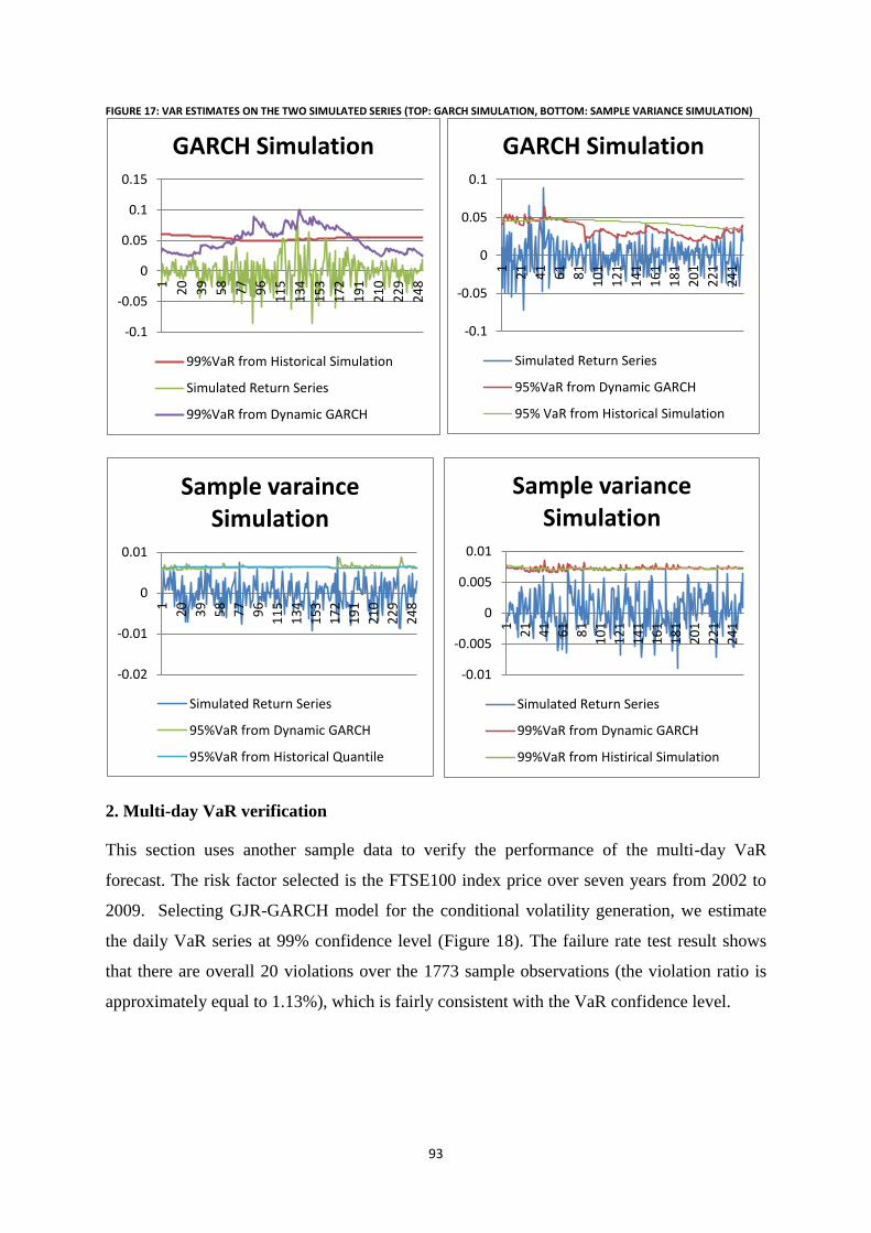
93

FIGURE 17: VAR ESTIMATES ON THE TWO SIMULATED SERIES (TOP: GARCH SIMULATION, BOTTOM: SAMPLE VARIANCE SIMULATION)

2. Multi-day VaR verification

This section uses another sample data to verify the performance of the multi-day VaR

forecast. The risk factor selected is the FTSE100 index price over seven years from 2002 to

2009. Selecting GJR-GARCH model for the conditional volatility generation, we estimate

the daily VaR series at 99% confidence level (Figure 18). The failure rate test result shows

that there are overall 20 violations over the 1773 sample observations (the violation ratio is

approximately equal to 1.13%), which is fairly consistent with the VaR confidence level.

-0.1

-0.05

0

0.05

0.1

0.15

1

20

39

58

77

96

11

5

13

4

15

3

17

2

19

1

21

0

22

9

24

8

GARCH Simulation

99%VaR from Historical Simulation

Simulated Return Series

99%VaR from Dynamic GARCH

-0.1

-0.05

0

0.05

0.1

1

21

41

61

81

10

1

12

1

14

1

16

1

18

1

20

1

22

1

24

1

GARCH Simulation

Simulated Return Series

95%VaR from Dynamic GARCH

95% VaR from Historical Simulation

-0.02

-0.01

0

0.01

1

20

39

58

77

96

11

5

13

4

15

3

17

2

19

1

21

0

22

9

24

8

Sample varaince Simulation

Simulated Return Series

95%VaR from Dynamic GARCH

95%VaR from Historical Quantile

-0.01

-0.005

0

0.005

0.01

1

21

41

61

81

10

1

12

1

14

1

16

1

18

1

20

1

22

1

24

1

Sample variance Simulation

Simulated Return Series

99%VaR from Dynamic GARCH

99%VaR from Histirical Simulation

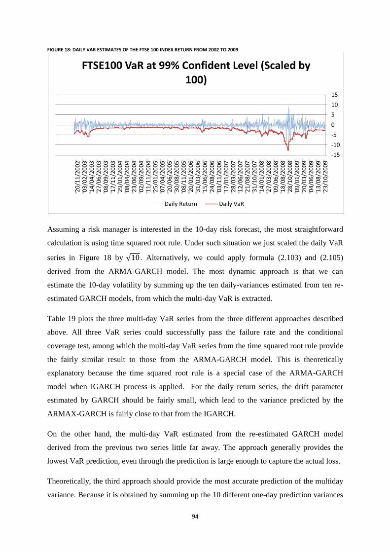
94

FIGURE 18: DAILY VAR ESTIMATES OF THE FTSE 100 INDEX RETURN FROM 2002 TO 2009

Assuming a risk manager is interested in the 10-day risk forecast, the most straightforward

calculation is using time squared root rule. Under such situation we just scaled the daily VaR

series in Figure 18 by . Alternatively, we could apply formula (2.103) and (2.105)

derived from the ARMA-GARCH model. The most dynamic approach is that we can

estimate the 10-day volatility by summing up the ten daily-variances estimated from ten re-

estimated GARCH models, from which the multi-day VaR is extracted.

Table 19 plots the three multi-day VaR series from the three different approaches described

above. All three VaR series could successfully pass the failure rate and the conditional

coverage test, among which the multi-day VaR series from the time squared root rule provide

the fairly similar result to those from the ARMA-GARCH model. This is theoretically

explanatory because the time squared root rule is a special case of the ARMA-GARCH

model when IGARCH process is applied. For the daily return series, the drift parameter

estimated by GARCH should be fairly small, which lead to the variance predicted by the

ARMAX-GARCH is fairly close to that from the IGARCH.

On the other hand, the multi-day VaR estimated from the re-estimated GARCH model

derived from the previous two series little far away. The approach generally provides the

lowest VaR prediction, even through the prediction is large enough to capture the actual loss.

Theoretically, the third approach should provide the most accurate prediction of the multiday

variance. Because it is obtained by summing up the 10 different one-day prediction variances

-15

-10

-5

0

5

10

15

'23

/10

/20

09

' '1

3/0

8/2

00

9'

'04

/06

/20

09

' '2

0/0

3/2

00

9'

'09

/01

/20

09

' '2

8/1

0/2

00

8'

'18

/08

/20

08

' '0

9/0

6/2

00

8'

'27

/03

/20

08

' '1

4/0

1/2

00

8'

'31

/10

/20

07

' '2

1/0

8/2

00

7'

'12

/06

/20

07

' '2

8/0

3/2

00

7'

'17

/01

/20

07

' '0

3/1

1/2

00

6'

'24

/08

/20

06

' '1

5/0

6/2

00

6'

'31

/03

/20

06

' '2

0/0

1/2

00

6'

'08

/11

/20

05

' '3

0/0

8/2

00

5'

'20

/06

/20

05

' '0

7/0

4/2

00

5'

'25

/01

/20

05

' '1

1/1

1/2

00

4'

'02

/09

/20

04

' '2

3/0

6/2

00

4'

'08

/04

/20

04

' '2

9/0

1/2

00

4'

'17

/11

/20

03

' '0

8/0

9/2

00

3'

'27

/06

/20

03

' '1

4/0

4/2

00

3'

'03

/02

/20

03

' '2

0/1

1/2

00

2'

FTSE100 VaR at 99% Confident Level (Scaled by 100)

Daily Return Daily VaR

95

based on the dynamically updated GARCH models. However, the empirical results shows

that the multi-day VaR estimates generated from the single GARCH model are even more

conservative than those from dynamic updated GARCH model. From this perspective, it

seems that time squared root rule should be preferred for the passive risk managers, since it

could actually provide a fast and quite conservative and safe risk measurement.

FIGURE 19: 10-DAY VAR FORECAST SERIES OF FTSE 100 INDEX FROM 2002 TO 2009

3.7.3 Empirical results summary

Apply the back testing approaches to the selected risk models, the empirical results show that

the performance of the VaR model is highly depend on how well it could capture the current

market volatility. VaR from the re-estimated GARCH models should be fairly dynamic and

appropriate for the time varying market risk assessment. However, due to the computation

cumbersome, it is not necessary to be applied at any kind of the market condition. The

simulated scenarios analysis show that if the changes of the return series are fairly stable, this

VaR model do nothing better than the VaR from the historical approximation. The VaR from

historical quantile is preferable under such case due to its speed and convenience.

Furthermore, the back-testing result shows that if the daily VaR series are generated from the

appropriate GARCH model, the multiday VaR prediction from both the time squared root

rule and the ARXA-GARCH model are safe to capture the actual loss. While the first

approach is based on the information up to the initial forecast date, the second one requires

the information up to the day just before the forecast horizon. Although the second approach

is theoretically more accurate than the first approach since the predicted variance is obtained

by summing up the 10 updated one-day prediction variances based on the re-estimated

-0.5

-0.4

-0.3

-0.2

-0.1

0

0.1

0.2

0.3 10 Day VaR at 99% Confident Level

Multi-day VaR from Time Squared Root

Multi-day VaR from General Formula

96

GARCH( the first one is estimated by the single GARCH model), the empirical result shows

that the time-squared root rule could actually provide a more conservative risk measurement.

Therefore for passive risk manger, it seems that time squared rule could be safe trusted, since

it is a both easy implemented and conservative risk measurement.

97

4. Two Step Dynamic Adjusted VaR model

Motivated by the idea of fitting the historical VaR estimates into pre-specified time series

model as proposed in chapter two, this chapter proposed a new developed VaR model, which

integrate the GARCH volatility and quantile regression technique. More explicitly, we

present a two-step dynamic adjusted VaR model, in which the VaR series generated from the

dynamic GARCH model in the first step are fitted into a pre-specified quantile regression for

the second adjustment. The back-testing results based on both real and simulated data shows

that the VaR series generated from this model could more efficient capture the time varying

risk evolution than the traditional CAViaR model, where efficiency here is measured by the

total sum of the violation and the over-prediction over the realized returns during the testing

period. Furthermore, given that the estimation of the multiday distribution is more complex

than that from daily basis, we shows that this model is particularly useful in the multi-period

VaR prediction, since the conditional distribution from this model encompass more

information than the time squared root rule.

4.1 Introduction

VaR is by definition a certain quantile of the return’s distribution over fixed holding period

and at given confidence level. This quantitative approach has rapidly becomes the benchmark

measurement of the market risk in the financial field over the last several decades. Different

VaR models are essentially due to the different ways of the distribution modeling. For

instance, early risk measurement is based on the parametric distribution and i.i.d. framework;

by evolution, researchers turn their attention to the conditional distribution and time series

model. The estimation of the conditional distributions also varies lots. For instance, standard

industry risk measurement system such as Riskmetrics mainly focuses on the parametric

approach. Boudoukh, Richardon and Whitelaw (1998) developed a hybrid estimation

approach combining the exponential smoothing process and historical simulation. Inspired by

the Extreme Value Theory, McNeil and Frey (2000) proposed a semi-parametric approach

combining GARCH modeling and Extreme Value Theory, which concentrates on the

asymptotic form of the tail rather than the whole distribution. Most recently, Cai and Wang

(2008) suggest a new nonparametric estimation approach, which integrate the Weighted

Nadaraya Watson estimator and Double kernel local linear estimator from Yu and Jones

(1998). Schaumburg refines this approach by adding the quantile regression of the extreme

value in their working paper in 2010.

98

In spite of various estimation approaches, none of the VaR models developed so far provides

a satisfactory solution for the dynamic risk adjustment. The reason is largely due to that

conditional distribution of the returns changes over time. It is statistically challenging to find

a suitable model to fit the time varying conditional distribution. Generally speaking, existing

dynamic adjustment can be classified into two categories according to their different

treatment of the time varying conditional distribution, which are:

1. Apply volatility model to adjust the conditional volatility (see, e.g., GARCH model

by Nelson, 1993; Wilson, 1994; Stochastic volatility model by Taylor and Ruiz,1994)

and VaR is calculated as the product of the dynamic volatility and the standard normal

quantile

2. Apply nonparametric approach to estimate the conditional distribution. Dynamic VaR

could be generated using quantile regression technique (see, e.g., CAViaR model by

Engle, 2002)

This chapter concentrates on the dynamic VaR adjustment and we propose a new dynamic

VaR generating process by integrating the GARCH volatility and quantile regression

technique. The back-testing results show that this model has its own superiority over the

tradition CAViaR models in capturing the dynamic evolution of the conditional distribution.

Besides, this approach is particularly useful for the multi-day VaR prediction, given that the

multiday distribution is more difficult to model and highly subject to estimation errors.

The chapter is structured as follows: Section 2 provides a brief illustration of the existing

dynamic VaR models. In section 3 we introduce the new dynamic VaR generating process in

this research. Section 4 implements the model application using both real and the simulated

data. Sections 5 provide the conclusion and some further implications.

4.2 Brief review of the Dynamic adjustment approach

Statistically, VaR is closely related to the conditional quantile of the return distribution.

Despite of this simple concept, the estimation is a fairly challenging task, not only because

the typical financial returns are characterized by the non-normal distribution with heavy tail;

but also the conditional distribution changes over time.

According to the different treatment of the time varying conditional distribution, empirical

research can be divided into two categories: one is focus on the dynamic adjustment of the

conditional volatility and the other is focus on the dynamic adjustment of the conditional

quantile. Currently there is no agreement on which approach is superior since it is not easy to

99

separate these two effects on the time varying conditional distribution. The following part of

the section provides a more detailed explanation of these two approaches.

4.2.1 Dynamic VaR on the time-varying volatility

Dynamic adjustment of the conditional volatility involves using time series model. Consider

the following model for the return :

(4.1)

where is the conditional volatility at time and , , , are parameters to be

estimated.

Under the assumption that model is correctly specified, the standard residual series follows

Gaussian process and at any time , the conditional distribution (denote ) has

the same form as . Re-writing in form of the conditional moment as:

(4.2)

where:

(4.3)

Taking the VaR operator to both sides of equation (4.2) we have:

(4.4)

Given that is a i.i.d. series and the conditional mean of the asset is fairly small and

constant, equation (4.4) shows that the dynamicity of the VaR estimate is mainly driven by

the time varying conditional volatility .

A further improvement of (4.4) could be made by the selecting a appropriate . . At

the low confidence level such as 95%, the standard normal or student could be used. If a

high confidence level of VaR is required (such as 99% or more), can be more

conservatively estimated by the Peaks over Threshold model derived from Extreme Value

Theory. This approach is proposed by McNeil and Frey (2000), in which the exceeded

100

standard residual over the given threshold is modeled by Generalized Pareto distribution.

The could be estimated by following formula:

(4.5)

where and are the parameters from Generalized Pareto distribution and is the selected

threshold.

The VaR series could therefore be generated by combining (4.4) and (4.5).

To summarize, the Dynamic VaR on time varying volatility adjust the VaR estimate in two

aspects: On one hand, the conditional volatility estimation from the pre-specified time series

model is dynamically updated; On the other hand, could also be updated

dynamically based on the standard residual series extracted from the conditional volatility

model.

4.2.2 Dynamic VaR on time-varying quantile

Alternatively, Engle and Manganelli (2004) proposed a conditional autoregressive

specification of VaR, so called CAViaR model, for dynamic VaR generation. This model is

motivated by the quantile regression technique introduced by Koenker and Zhao (1996).

Since VaR is statistically a quantile estimate, quantile regression model could be directly

applied to the VaR generation. The general CAViaR model by Engle can be expressed as:

(4.6)

where is a function of finite number of lagged values of the exogenous variables

and autoregressive terms ensure that the estimated quantile changes smoothly

over time.

Particularly, Engel propose following four types of models, which are:

Adaptive model:

(4.7)

Symmetric Absolute Value: (4.8)

Asymmetric Slope: (4.9)

Indirect GARCH:

(4.10)

101

The Adaptive model (4.7) encompass a self-correction property, in which G is some positive

finite number controlling the correction degree. For instance, once the actual loss exceed the

VaR estimate in the previous period, the second term of the adaptive model will become

positive which will increase the VaR estimate in the next period , and vice versa. Both

symmetric and indirect GARCH model have mean reverting property and respond

symmetrically to the past returns. The asymmetric slope model, on the other hand, takes into

account the asymmetric effect of the returns on the quantile forecast.

Unlike the GARCH types of model mentioned in 4.2.1, there is no assumption on the

distribution of the residual terms in the Engle’s CAViaR models. The only assumption under

this framework is that the quantile process is correctly specified. Moreover, even if the

quantile process is misspecified, Kim and White (2002) shows that the minimization of the

quantile regression objective function (2.19) by Koenker will still ensure the consistency and

asymptotic normality property.

4.3 Two-Step Dynamic Adjusted VaR model

This section presents a new dynamic VaR generating process from our research. More

explicitly, Instead of applying the autoregressive terms in Engel’s CAViaR,

we generate a new repressor using the GARCH types of volatility. By doing so, we believe

the original CAViaR specification could possibly be simplified, because the time varying

conditional volatility by GARCH model should already contain certain effect represented by

the existing exogenous variables in the original CAViaR model. For instance, if time varying

conditional volatilities are generated from the dynamic EGARCH model, the asymmetric

specification in the Asymmetric Slope-CAViaR model could possibly be removed, because

conditional volatilities extracted from the EGACH process has already take account into this

effect. Moreover, we could therefore add some new exogenous variables whose effects have

not been considered in the original CAViaR model. This process is so called two-step

dynamic-adjustment process, in which the conditional VaR series generated from the

dynamic volatility model in the first step is re-adjusted using quantile regression technique in

the second step.

Particularly, we specify the following quantile regression model for VaR generation, which is:

102

(4.11)

where:

, are volatility and residual quantile estimated from GARCH model.

is the estimated expected shortfall

is the maximum loss the risk manager could withstand.

is the indicator function.

There are three explanatory variables appear in this regression specification, which are:

Parametric VaR estimate from GARCH model : The product of and

is the VaR estimate from GARCH model at time

Self-correction indicator 3 : A variable which increase the VaR if the previous VaR

estimate have been violated and decrease the VaR if the previous VaR estimate

haven’t been broke.

Panic selling effect4 : an indicator variable which takes value equal to 1 if the

previous daily return is below maximum tolerate loss.

Compared to the CAViaR models proposed by Engle, the model (4.11) has three changes:

Firstly, the autoregressive terms has been replaced by the parametric VaR

estimate ( ) from GARCH model. Secondly, the constant in the adaptive

model which controls the degree of self-correction is replaced by the estimated expected

shortfall

. This variable reacts different to the return on the time which is close to

the estimated

or extremely far from the estimated

. Finally, a new exogenous

variable is added into the regression. The dummy variable could serve as

a complementary cushion when the asset undertakes serious crash beyond the manager’s

tolerance.

There are several motivations to apply this model in practice: First, since the autoregressive

term

are replaced by the estimated from GARCH types of model,

both time varying volatility and time varying quantile have been taken into account by

103

regression (4.11) . Secondly, estimated from the GARCH model contains

certain effect about the nonlinear evolution of the conditional quantile regression which is

ignored in the linear specification of the traditional CAViaR model. This adjustment should

improve the accuracy of the VaR model.

Thirdly, the time varying

replace the constant G in the adaptive CAViaR model. The

motivation of using

is that it is fairly sensitive to the estimated value of

.

Unlike constant smoothing factor G,

increase the value when

estimate increase

and decrease the value when

estimate decrease. This adjustment try to alleviate the

problem from Adaptive CAViaR model that it will increase the VaR estimate by the same

amount regardless of whether the returns exceed the previous VaR estimate by small or by

large amount.

The research applies two alternative processes for the

generation. At , the

empirical quantile is used, in which

is obtained by numerically integrating the excess

area of the kernel density over the estimated . The selection of the density’s

bandwidth is based on the Plug-in method by Fan & Yao (2003), in which the optimum

bandwidth is obtained by minimize the Mean Integrated Squared Error. Particularly, Fan &

Yao provide the optimum bandwidth selection criterion as following:

(4.13)

where is the sample standard error and is the sample size

At , we apply extreme value theory and use the following formula derived by McNeil

and Frey (2000)from Generalized Pareto distribution(GPD):

(4.14)

where and are the scale and shape parameter estimated from GPD.

The purpose of applying two separate methods for

estimation is to improve the

accuracy at the different VaR confidence level. At the , the quantile from empirical

distribution could severs as a appropriate lower boarder for the true VaR. Give that the

is estimated using empirical distribution of standardised residuals at this

104

confidence level, the expected loss

could therefore be estimated by integrating the

excess tail area over the obtained . On the other hand, the effects of fat tail

becomes more important at the . Give the Extreme Value Theory has been applied

for at this confidence level, we apply the same approach to estimate the

for consistence.

Finally, the selected exogenous variable could serve as a complementary cushion when the

asset undertakes serious crash beyond the manager’s tolerance and hence improve the

accuracy of the risk prediction under the extreme market condition.

This dynamic adjustment idea can be applied for multiday VaR generation as well. To

generate a VaR forecast on the initial date , we first estimate a historical

variance series from GARCH types of models. The corresponding residual series

from GARCH model could be used to generate the multiday series

using the power scaling law proposed by McNeil and Fry (2000), which states:

where is the scale parameter whose value depends on the current volatility level of the

overall market21

Finally, the multiday volatility and VaR series are fitted into the following Quantile

regression model and generate the multi-day VaR forecast:

(4.15)

where is the cumulative maximum loss over the latest that the risk

manager could tolerate

To summarize this process, we first generate the conditional VaR series on time varying

volatility based on the sample historical data. The dynamicity of the VaR series in this step is

mainly driven by the time varying conditional volatility estimated from the corresponding

21

See detailed value selection of in McNeil and Frey’s research (2000)

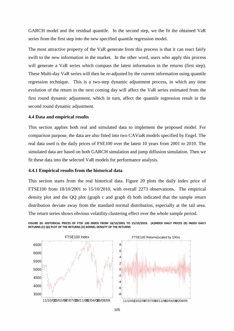
105

GARCH model and the residual quantile. In the second step, we the fit the obtained VaR

series from the first step into the new specified quantile regression model.

The most attractive property of the VaR generate from this process is that it can react fairly

swift to the new information in the market. In the other word, users who apply this process

will generate a VaR series which compass the latest information in the returns (first step).

These Multi-day VaR series will then be re-adjusted by the current information using quantile

regression technique. This is a two-step dynamic adjustment process, in which any time

evolution of the return in the next coming day will affect the VaR series estimated from the

first round dynamic adjustment, which in turn, affect the quantile regression result in the

second round dynamic adjustment.

4.4 Data and empirical results

This section applies both real and simulated data to implement the proposed model. For

comparison purpose, the data are also fitted into two CAViaR models specified by Engel. The

real data used is the daily prices of FSE100 over the latest 10 years from 2001 to 2010. The

simulated data are based on both GARCH simulation and jump diffusion simulation. Then we

fit these data into the selected VaR models for performance analysis.

4.4.1 Empirical results from the historical data

This section starts from the real historical data. Figure 20 plots the daily index price of

FTSE100 from 18/10/2001 to 15/10/2010, with overall 2273 observations. The empirical

density plot and the QQ plot (graph c and graph d) both indicated that the sample return

distribution deviate away from the standard normal distribution, especially at the tail area.

The return series shows obvious volatility clustering effect over the whole sample period.

FIGURE 20: HISTORICAL PRICES OF FTSE 100 INDEX FROM 18/10/2001 TO 15/10/2010. (A)INDEX DAILY PRICES (B) INDEX DAILY RETURNS (C) QQ PLOT OF THE RETURNS (D) KERNEL DENSITY OF THE RETURNS

11/10/0223/02/0407/07/0519/11/0602/04/0815/08/09

3500

4000

4500

5000

5500

6000

6500

FTSE100 Index

11/10/0223/02/0407/07/0519/11/0602/04/0815/08/09

-8

-6

-4

-2

0

2

4

6

8

FTSE100 Returns(scaled by 100x)

106

Figure 21 present the sample ACF of the returns and the squared returns over the entire

sample period, from which we found that the return series shows no serious autocorrelation

while the autocorrelation of the squared returns are relatively high at all 40 selected lags.

This indicates that the selected return series are series-unrelated but not independent, which

confirms the existence of the GARCH effect. Taking into account of this property, the

research fit the return series into several types of GARCH model.22

The model parameters are

re-estimated at daily frequency with 1-year data window (252 observations). For each set of

the parameters, the conditional variance prediction one day ahead is provided. The

conditional VaR series is generated by combining the predicted conditional volatility from

GARCH model and corresponding residual quantile. Particularly, at 99% confidence level,

the residual quantile is modeled by EVT, while at 95% confidence level it is generated from

the same distribution specified in the corresponding GARCH model.

FIGURE 21: SAMPLE RETURN ACF AND SQUARED RETURN PACF OF FTSE 100 RETURNS FROM 18/10/2001 TO 15/10/2010

22

Several GARCH types of models are used including Standard GARCH, GJR-Asymmetric GARCH and EGARCH. The selection of best GARCH was based on the Both Akaike-AIC and Schwarz-BIC criterion. See figure 22

-0.1

0-0

.05

0.0

00.0

50.1

0

Auto

co

rrela

tio

ns o

f R

etu

rn

0 10 20 30 40Lag

Bartlett's formula for MA(q) 95% confidence bands

Return ACF

-0.1

00.0

00.1

00.2

00.3

00.4

0

Auto

corr

ela

tions o

f re

turn

1

0 10 20 30 40Lag

Bartlett's formula for MA(q) 95% confidence bands

Squared return ACF

-6 -4 -2 0 2 4 6

-6

-4

-2

0

2

4

6

FTSE100 Index standard Returns

No

rma

l

QQ plot

-15 -10 -5 0 5 100

0.05

0.1

0.15

0.2

0.25

0.3

0.35

0.4

0.45FTSE100 Index - Return Density

Kernel density

Normal density

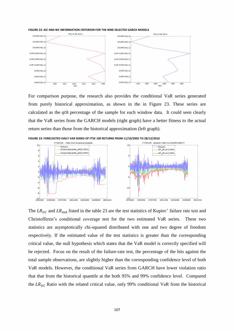
107

FIGURE 22: AIC AND BIC INFORMATION CRITERION FOR THE NINE SELECTED GARCH MODELS

For comparison purpose, the research also provides the conditional VaR series generated

from purely historical approximation, as shown in the in Figure 23. These series are

calculated as the percentage of the sample for each window data. It could seen clearly

that the VaR series from the GARCH models (right graph) have a better fitness to the actual

return series than those from the historical approximation (left graph).

FIGURE 23: FORECASTED DAILY VAR SERIES OF FTSE 100 RETURNS FROM 11/10/2002 TO 28/12/2010

The and listed in the table 23 are the test statistics of Kupiec’ failure rate test and

Christofferen’s conditional coverage test for the two estimated VaR series. These two

statistics are asymptotically chi-squared distributed with one and two degree of freedom

respectively. If the estimated value of the test statistics is greater than the corresponding

critical value, the null hypothesis which states that the VaR model is correctly specified will

be rejected. Focus on the result of the failure-rate test, the percentage of the hits against the

total sample observations, are slightly higher than the corresponding confidence level of both

VaR models. However, the conditional VaR series from GARCH have lower violation ratio

that that from the historical quantile at the both 95% and 99% confidence level. Compared

the Ratio with the related critical value, only 99% conditional VaR from the historical

-330 -325 -320 -315 -310 -305GARCH(1,1)

GARCH(2,1)

GARCH(1,2)

GJR-GARCH(1,1)

GJR-GARCH(2,1)

GJR-GARCH(1,2)

EGARCH(1,1)

EGARCH(2,1)

EGARCH(1,2)Plot of the AICs

AIC

-310 -305 -300 -295 -290 -285GARCH(1,1)

GARCH(2,1)

GARCH(1,2)

GJR-GARCH(1,1)

GJR-GARCH(2,1)

GJR-GARCH(1,2)

EGARCH(1,1)

EGARCH(2,1)

EGARCH(1,2)Plot of the BICs

BIC

11/10/02 23/02/04 07/07/05 19/11/06 02/04/08 15/08/09 28/12/10-10

-8

-6

-4

-2

0

2

4

6

8

10FTSE100 - VaRs from Empirical Quantile

Returns

EmpiricalQuantileVaR(CL95%)

EmpiricalQuantileVaR(CL99%)

11/10/02 23/02/04 07/07/05 19/11/06 02/04/08 15/08/09 28/12/10-15

-10

-5

0

5

10FTSE100 - dynamic VaRs for EGARCH&EVT

Returns

SPVaR at CL95%

SPVaR at CL99%

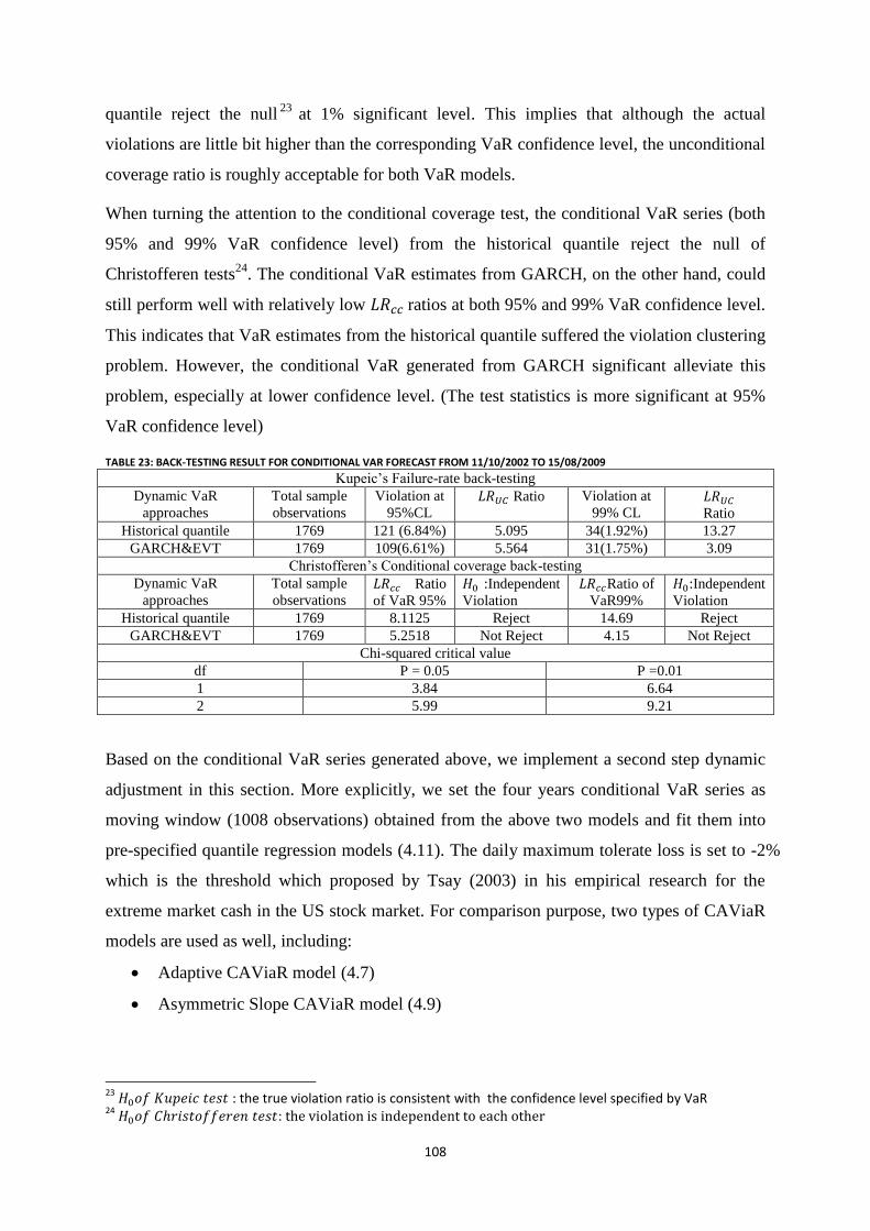
108

quantile reject the null23

at 1% significant level. This implies that although the actual

violations are little bit higher than the corresponding VaR confidence level, the unconditional

coverage ratio is roughly acceptable for both VaR models.

When turning the attention to the conditional coverage test, the conditional VaR series (both

95% and 99% VaR confidence level) from the historical quantile reject the null of

Christofferen tests24

. The conditional VaR estimates from GARCH, on the other hand, could

still perform well with relatively low ratios at both 95% and 99% VaR confidence level.

This indicates that VaR estimates from the historical quantile suffered the violation clustering

problem. However, the conditional VaR generated from GARCH significant alleviate this

problem, especially at lower confidence level. (The test statistics is more significant at 95%

VaR confidence level)

TABLE 23: BACK-TESTING RESULT FOR CONDITIONAL VAR FORECAST FROM 11/10/2002 TO 15/08/2009

Kupeic’s Failure-rate back-testing

Dynamic VaR

approaches

Total sample

observations

Violation at

95%CL Ratio Violation at

99% CL

Ratio

Historical quantile 1769 121 (6.84%) 5.095 34(1.92%) 13.27

GARCH&EVT 1769 109(6.61%) 5.564 31(1.75%) 3.09

Christofferen’s Conditional coverage back-testing

Dynamic VaR

approaches

Total sample

observations Ratio

of VaR 95%

:Independent

Violation

Ratio of

VaR99%

:Independent

Violation

Historical quantile 1769 8.1125 Reject 14.69 Reject

GARCH&EVT 1769 5.2518 Not Reject 4.15 Not Reject

Chi-squared critical value

df P = 0.05 P =0.01

1 3.84 6.64

2 5.99 9.21

Based on the conditional VaR series generated above, we implement a second step dynamic

adjustment in this section. More explicitly, we set the four years conditional VaR series as

moving window (1008 observations) obtained from the above two models and fit them into

pre-specified quantile regression models (4.11). The daily maximum tolerate loss is set to -2%

which is the threshold which proposed by Tsay (2003) in his empirical research for the

extreme market cash in the US stock market. For comparison purpose, two types of CAViaR

models are used as well, including:

Adaptive CAViaR model (4.7)

Asymmetric Slope CAViaR model (4.9)

23

: the true violation ratio is consistent with the confidence level specified by VaR 24

: the violation is independent to each other

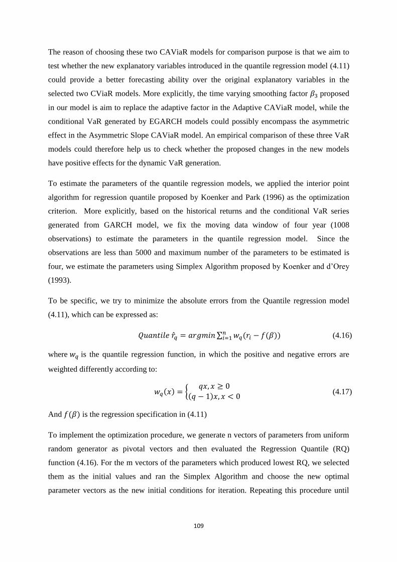
109

The reason of choosing these two CAViaR models for comparison purpose is that we aim to

test whether the new explanatory variables introduced in the quantile regression model (4.11)

could provide a better forecasting ability over the original explanatory variables in the

selected two CViaR models. More explicitly, the time varying smoothing factor proposed

in our model is aim to replace the adaptive factor in the Adaptive CAViaR model, while the

conditional VaR generated by EGARCH models could possibly encompass the asymmetric

effect in the Asymmetric Slope CAViaR model. An empirical comparison of these three VaR

models could therefore help us to check whether the proposed changes in the new models

have positive effects for the dynamic VaR generation.

To estimate the parameters of the quantile regression models, we applied the interior point

algorithm for regression quantile proposed by Koenker and Park (1996) as the optimization

criterion. More explicitly, based on the historical returns and the conditional VaR series

generated from GARCH model, we fix the moving data window of four year (1008

observations) to estimate the parameters in the quantile regression model. Since the

observations are less than 5000 and maximum number of the parameters to be estimated is

four, we estimate the parameters using Simplex Algorithm proposed by Koenker and d’Orey

(1993).

To be specific, we try to minimize the absolute errors from the Quantile regression model

(4.11), which can be expressed as:

(4.16)

where is the quantile regression function, in which the positive and negative errors are

weighted differently according to:

(4.17)

And is the regression specification in (4.11)

To implement the optimization procedure, we generate n vectors of parameters from uniform

random generator as pivotal vectors and then evaluated the Regression Quantile (RQ)

function (4.16). For the m vectors of the parameters which produced lowest RQ, we selected

them as the initial values and ran the Simplex Algorithm and choose the new optimal

parameter vectors as the new initial conditions for iteration. Repeating this procedure until

110

the convergence criterion is satisfied and we selected the parameter vector as the final

optimal one. The value of n and m is set similar to the Engel and Manganelli (2004).

As an example, we report the Least Absolute Deviation estimates and the relevant statistics

for the three models using data window from 11/10/02 to 11/10/06 in Table 24 and Table 25.

For each model, the table reports the LAD estimated parameters, the corresponding standard

errors25

, two tailed P-values and .

Several points are worth to be mentioned from these two tables: Firstly, under both 5% and 1%

quantile level, the two step dynamic adjusted VaR (TSDA-VaR) model has a higher than

Adaptive-CAViaR and Asymmetric Slope-CAViaR model, which confirms the goodness of

fit improved by the new model. Secondly, the coefficients of the auto-correction variable beta

3 and the new exogenous variable beta 4 in the TSDA-VaR model are both fairly significant

at 5% significant level, which confirms the explanatory power of these two exogenous

variables. Thirdly, for 1% quantile level, the coefficient of the modified adaptive factor beta 3

in TSDA-CAViaR model, which represent the time varying self-correction effect, is more

significant than the adaptive factor beta 1 in the Adaptive-CAViaR model, confirming the

robustness of the modified adaptive factor in the dynamic VaR generation.

FIGURE 24: ESTIMATED DAILY EXPECTED SHORTFALL OF FTSE 100 INDEX FROM 11/10/2002 TO 15/08/2009

25

See detailed explanation of the statistics in Koenker(2005)

-25

-20

-15

-10

-5

0

5

10

15

1

55

10

9

16

3

21

7

27

1

32

5

37

9

43

3

48

7

54

1

59

5

64

9

70

3

75

7

81

1

86

5

91

9

97

3

10

27

10

81

11

35

11

89

12

43

12

97

13

51

14

05

14

59

15

13

15

67

16

21

16

75

17

29

FTSE 100 Expected Shortfall(%) estimate at 95% and 99% Confidence Level

return Expected Shortfall at 95% CL Expected Shortfall at 99% CL

111

TABLE 24: QUANTILE REGRESSION RESULT USING WINDOW DATA FROM 11/10/02 TO 11/10/06 ( )

Dynamic VaR generating at 95% confidence level ( )

Results of quantile Regression : TSDA-VaR

Explanatory Variables Coefficients SE.ker t.ker P.ker

Constants (Beta 1) -0.3741 0.0809 -4.6238 0.0000

Beta 2 0.8367 0.0325 25.7449 0

Beta 3 -1.1972 0.3462 -3.4584 0.0006

Beta 4 -0.4974 0.2748 -1.8100 0.0705

Pseudo 0.1742

Elapsed time 66.35seconds

Results of quantile Regression : Adaptive-CAViaR

Explanatory Variables Coefficients SE.ker t.ker P.ker

Beta 1 -1.0284 0.3546 2.9005 0.0038

Pseudo 0.0878

Elapsed time 25.830 seconds.

Results of quantile Regression : Asymmetric Slope-CAViaR

Explanatory Variables Coefficients SE. t.ker P.ker

Constants -0.3085 0.0971 -3.1771 0.0015

Beta 2 0.6992 0.0485 14.4036 0

Beta 3 -0.4115 0.0507 -8.1103 0.0000

Beta 4 0.3026 0.0676 4.4779 0.0000

Pseudo 0.0903

Elapsed time 28.21seconds TABLE 25: QUANTILE REGRESSION RESULT USING WINDOW DATA FROM 11/10/02 TO 11/10/06 ( )

Dynamic VaR generating at 99% confidence level( )

Results of quantile Regression : TSDA-VaR

Explanatory Variables Coefficients SE.ker t.ker P.ker

Constants (Beta 1) -0.6483 0.1020 -6.3539 0.0000

Beta 2 0.8650 0.0306 28.2932 0

Beta 3 -1.7003 0.5760 -2.9516 0.0032

Beta 4 -2.3783 0.5450 -4.3638 0.0000

Pseudo 0.3208

Elapsed time 72.45 seconds

Results of quantile Regression : Adaptive-CAVaiR

Explanatory Variables Coefficients SE.ker t.ker P.ker

Beta 1 -1.1426 0.7639 1.4959 0.1349

Pseudo 0.1450

Elapsed time 25.20seconds.

Results of quantile Regression : Asymmetric Slope-CAVaiR

Explanatory Variables Coefficients SE. t.ker P.ker

Constants (Beta 1) -0.5969 0.1296 -4.6047 0.0000

Beta 2 0.6998 0.0321 21.8314 0

Beta 3 -0.6917 0.0995 -6.9519 0.0000

Beta 4 1.0315 0.1139 9.0565 0

Pseudo 0.1929

Elapsed time 32.536916

112

In figure 25 we plot the daily dynamic VaR series at 95% and 99% confidence level predicted

from the three types of CAViaR models against the actual index returns. These series are

generated by moving the four window data at daily frequency and re-estimating the three

VaR models in the table 25. The overall looping process runs 1771 times and we take one -

day forecast from each loop to construct the dynamic VaR series. The overall VaR series

contained 1771 forecast spanning from 11/12/02 to 15/08/2009.

For back-testing purpose, this section compared the dynamic VaR series generated from the

above process and the actual return series over the same period from 11/12/02 to 15/08/2009.

The VaR model validation is checked by three back-testing models, which are

aforementioned failure rate test, conditional coverage test and Dynamic Quantile (DQ) test

proposed by Engel (2002). To briefly explain the DQ test, define the hit as an indicator

variable, which is expressed as:

(4.18)

If the VaR model is correctly specified, the hits should have expected value equal to with

no auto-correlation. Furthermore, the hits must be unpredictable conditional on the current

information. This non-predictability property can be tested by regressing the hits on several

selected explanatory variables, which is expressed as:

(4.19)

where are the lags of the Hits and is the actual return on time

Under the null hypothesis that the distribution of the hits is dependent on the past

observations, DQ statistics should follow Chi-squared distribution with k degree of freedom:

(4.20)

Where:

is the k-vector of the explanatory variables

is the DQ matrix26

26

The detailed proof of the DQ matrix could be found in Engle and Manganelli(2004)

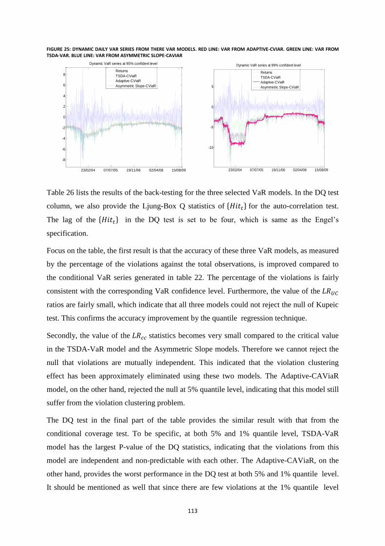
113

FIGURE 25: DYNAMIC DAILY VAR SERIES FROM THERE VAR MODELS. RED LINE: VAR FROM ADAPTIVE-CVIAR. GREEN LINE: VAR FROM TSDA-VAR. BLUE LINE: VAR FROM ASYMMETRIC SLOPE-CAVIAR

Table 26 lists the results of the back-testing for the three selected VaR models. In the DQ test

column, we also provide the Ljung-Box Q statistics of for the auto-correlation test.

The lag of the in the DQ test is set to be four, which is same as the Engel’s

specification.

Focus on the table, the first result is that the accuracy of these three VaR models, as measured

by the percentage of the violations against the total observations, is improved compared to

the conditional VaR series generated in table 22. The percentage of the violations is fairly

consistent with the corresponding VaR confidence level. Furthermore, the value of the

ratios are fairly small, which indicate that all three models could not reject the null of Kupeic

test. This confirms the accuracy improvement by the quantile regression technique.

Secondly, the value of the statistics becomes very small compared to the critical value

in the TSDA-VaR model and the Asymmetric Slope models. Therefore we cannot reject the

null that violations are mutually independent. This indicated that the violation clustering

effect has been approximately eliminated using these two models. The Adaptive-CAViaR

model, on the other hand, rejected the null at 5% quantile level, indicating that this model still

suffer from the violation clustering problem.

The DQ test in the final part of the table provides the similar result with that from the

conditional coverage test. To be specific, at both 5% and 1% quantile level, TSDA-VaR

model has the largest P-value of the DQ statistics, indicating that the violations from this

model are independent and non-predictable with each other. The Adaptive-CAViaR, on the

other hand, provides the worst performance in the DQ test at both 5% and 1% quantile level.

It should be mentioned as well that since there are few violations at the 1% quantile level

23/02/04 07/07/05 19/11/06 02/04/08 15/08/09

-8

-6

-4

-2

0

2

4

6

8

Dynamic VaR series at 95% confident level

Returns

TSDA-CViaR

Adaptive-CViaR

Asymmetric Slope-CViaR

23/02/04 07/07/05 19/11/06 02/04/08 15/08/09

-10

-5

0

5

Dynamic VaR series at 99% confident level

Returns

TSDA-CViaR

Adaptive-CViaR

Asymmetric Slope-CViaR

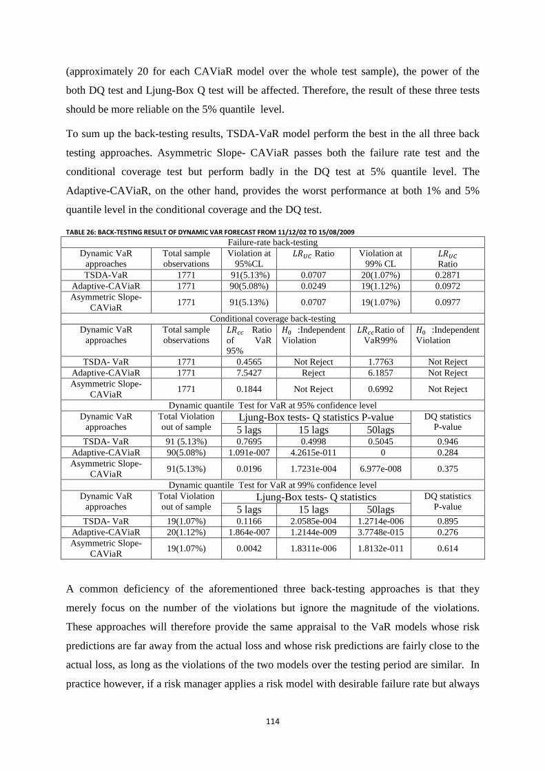
114

(approximately 20 for each CAViaR model over the whole test sample), the power of the

both DQ test and Ljung-Box Q test will be affected. Therefore, the result of these three tests

should be more reliable on the 5% quantile level.

To sum up the back-testing results, TSDA-VaR model perform the best in the all three back

testing approaches. Asymmetric Slope- CAViaR passes both the failure rate test and the

conditional coverage test but perform badly in the DQ test at 5% quantile level. The

Adaptive-CAViaR, on the other hand, provides the worst performance at both 1% and 5%

quantile level in the conditional coverage and the DQ test.

TABLE 26: BACK-TESTING RESULT OF DYNAMIC VAR FORECAST FROM 11/12/02 TO 15/08/2009

Failure-rate back-testing

Dynamic VaR

approaches

Total sample

observations

Violation at

95%CL Ratio Violation at

99% CL

Ratio

TSDA-VaR 1771 91(5.13%) 0.0707 20(1.07%) 0.2871

Adaptive-CAViaR 1771 90(5.08%) 0.0249 19(1.12%) 0.0972

Asymmetric Slope-

CAViaR 1771 91(5.13%) 0.0707 19(1.07%) 0.0977

Conditional coverage back-testing

Dynamic VaR

approaches

Total sample

observations Ratio

of VaR

95%

:Independent

Violation

Ratio of

VaR99%

:Independent

Violation

TSDA- VaR 1771 0.4565 Not Reject 1.7763 Not Reject

Adaptive-CAViaR 1771 7.5427 Reject 6.1857 Not Reject

Asymmetric Slope-

CAViaR 1771 0.1844 Not Reject 0.6992 Not Reject

Dynamic quantile Test for VaR at 95% confidence level

Dynamic VaR

approaches

Total Violation

out of sample Ljung-Box tests- Q statistics P-value DQ statistics

P-value 5 lags 15 lags 50lags TSDA- VaR 91 (5.13%) 0.7695 0.4998 0.5045 0.946

Adaptive-CAViaR 90(5.08%) 1.091e-007 4.2615e-011 0 0.284

Asymmetric Slope-

CAViaR 91(5.13%) 0.0196 1.7231e-004 6.977e-008 0.375

Dynamic quantile Test for VaR at 99% confidence level

Dynamic VaR

approaches

Total Violation

out of sample Ljung-Box tests- Q statistics DQ statistics

P-value 5 lags 15 lags 50lags TSDA- VaR 19(1.07%) 0.1166 2.0585e-004 1.2714e-006 0.895

Adaptive-CAViaR 20(1.12%) 1.864e-007 1.2144e-009 3.7748e-015 0.276

Asymmetric Slope-

CAViaR 19(1.07%) 0.0042 1.8311e-006 1.8132e-011 0.614

A common deficiency of the aforementioned three back-testing approaches is that they

merely focus on the number of the violations but ignore the magnitude of the violations.

These approaches will therefore provide the same appraisal to the VaR models whose risk

predictions are far away from the actual loss and whose risk predictions are fairly close to the

actual loss, as long as the violations of the two models over the testing period are similar. In

practice however, if a risk manager applies a risk model with desirable failure rate but always

115

provides too large VaR prediction compared to the actual loss when the violation does not

occur, there is obviously a deficiency loss because too many capital cushion is set to prevent

the unnecessary loss according to this model. Similarly, if a risk manager applies a risk model

with desirable failure rate but perform extremely badly when the violation does occur (has

too small VaR prediction compared to the actual loss), there will also be a potential danger to

implement this model because whenever the violation occurs, there will be a catastrophe to

the users.

For this reason, it is necessary to perform an additional efficiency test for the selected VaR

models. That is, how precise these models could capture the magnitude of the actual loss. In

this research we propose two efficiency measurements, which are:

Total violation errors: the sum of the violation magnitude (the difference between the

realized returns and the VaR estimates) over the testing period, conditional on that

violation does happen

Total over-prediction errors: the sum of the over-prediction magnitude (the difference

between the VaR estimates and the actual returns) over the testing period, conditional

on that violation doesn’t happen.

Table 27 summarizes the value of these two measures for the each selected VaR models. In

the last two columns of the table, we also list the value of the average magnitude. These

values are obtained by dividing the sum of the magnitude by the corresponding sample size.

For instance, the average magnitude of violation error is calculated as dividing the sum value

of violation error by the total number of the violations. Similarly, the average magnitude of

over-prediction error is calculated as dividing the sum value of over-prediction error by the

total number of the over-predictions.

As shown in the Table 27, the TSDA-VaR model has the lowest value of the total violation

errors and total over-prediction errors at the both 95% and 99% VaR confidence level. The

implication of this result could be seen from two aspects: On one hand, under the condition

that the violation occurs, TSDA- VaR could provide a larger VaR prediction than those from

other two CAViaR models; On the other hand, under the condition that the violation doesn’t

occur, VaR generated from TSDA-VaR is generally smaller than those from other two

models.

From the perspective of the average magnitude, the violation error from the TSDA-VaR

model (0.62%) is approximately 0.2% lower than those from the Adaptive-CAViaR and the

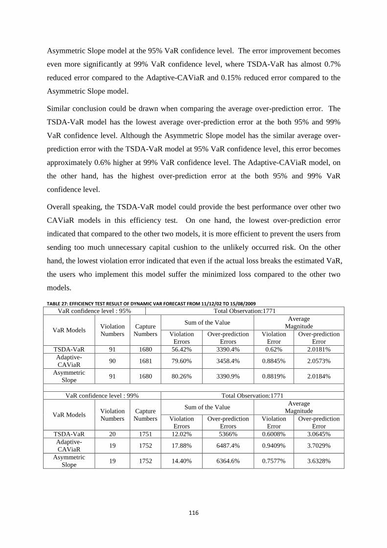
116

Asymmetric Slope model at the 95% VaR confidence level. The error improvement becomes

even more significantly at 99% VaR confidence level, where TSDA-VaR has almost 0.7%

reduced error compared to the Adaptive-CAViaR and 0.15% reduced error compared to the

Asymmetric Slope model.

Similar conclusion could be drawn when comparing the average over-prediction error. The

TSDA-VaR model has the lowest average over-prediction error at the both 95% and 99%

VaR confidence level. Although the Asymmetric Slope model has the similar average over-

prediction error with the TSDA-VaR model at 95% VaR confidence level, this error becomes

approximately 0.6% higher at 99% VaR confidence level. The Adaptive-CAViaR model, on

the other hand, has the highest over-prediction error at the both 95% and 99% VaR

confidence level.

Overall speaking, the TSDA-VaR model could provide the best performance over other two

CAViaR models in this efficiency test. On one hand, the lowest over-prediction error

indicated that compared to the other two models, it is more efficient to prevent the users from

sending too much unnecessary capital cushion to the unlikely occurred risk. On the other

hand, the lowest violation error indicated that even if the actual loss breaks the estimated VaR,

the users who implement this model suffer the minimized loss compared to the other two

models.

TABLE 27: EFFICIENCY TEST RESULT OF DYNAMIC VAR FORECAST FROM 11/12/02 TO 15/08/2009

VaR confidence level : 95% Total Observation:1771

VaR Models Violation

Numbers

Capture

Numbers

Sum of the Value Average

Magnitude

Violation

Errors

Over-prediction

Errors

Violation

Error

Over-prediction

Error

TSDA-VaR 91 1680 56.42% 3390.4% 0.62% 2.0181%

Adaptive-

CAViaR 90 1681 79.60% 3458.4% 0.8845% 2.0573%

Asymmetric

Slope 91 1680 80.26% 3390.9% 0.8819% 2.0184%

VaR confidence level : 99% Total Observation:1771

VaR Models Violation

Numbers

Capture

Numbers

Sum of the Value Average

Magnitude

Violation

Errors

Over-prediction

Errors

Violation

Error

Over-prediction

Error

TSDA-VaR 20 1751 12.02% 5366% 0.6008% 3.0645%

Adaptive-

CAViaR 19 1752 17.88% 6487.4% 0.9409% 3.7029%

Asymmetric

Slope 19 1752 14.40% 6364.6% 0.7577% 3.6328%

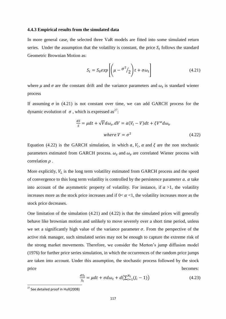
117

4.4.3 Empirical results from the simulated data

In more general case, the selected three VaR models are fitted into some simulated return

series. Under the assumption that the volatility is constant, the price follows the standard

Geometric Brownian Motion as:

(4.21)

where and are the constant drift and the variance parameters and is standard wiener

process

If assuming in (4.21) is not constant over time, we can add GARCH process for the

dynamic evolution of , which is expressed as27

:

(4.22)

Equation (4.22) is the GARCH simulation, in which , , and are the non stochastic

parameters estimated from GARCH process. and are correlated Wiener process with

correlation .

More explicitly, is the long term volatility estimated from GARCH process and the speed

of convergence to this long term volatility is controlled by the persistence parameter . take

into account of the asymmetric property of volatility. For instance, if >1, the volatility

increases more as the stock price increases and if 0< <1, the volatility increases more as the

stock price decreases.

One limitation of the simulation (4.21) and (4.22) is that the simulated prices will generally

behave like brownian motion and unlikely to move severely over a short time period, unless

we set a significantly high value of the variance parameter . From the perspective of the

active risk manager, such simulated series may not be enough to capture the extreme risk of

the strong market movements. Therefore, we consider the Merton’s jump diffusion model

(1976) for further price series simulation, in which the occurrences of the random price jumps

are taken into account. Under this assumption, the stochastic process followed by the stock

price becomes:

(4.23)

27

See detailed proof in Hull(2008)

118

where follows Poisson process with intensity and is non-negative iid series.

follows Laplacian distribution with the following probability density function:

(4.24)

where is the expected value of the jump size and is the volatility of the jump.

Under the Poisson distribution, the probability of one jump under the time interval

is equal to . The change of the price under such small time is therefore given by:

,

(4.25)

Solve the differential equation (4.23) we can obtain the following stochastic jump diffusion

equation:

(4.26)

Table 28 lists the value of the input parameters we set for the three types of simulation

process (4.24), (4.25) and (4.29). Each value of the parameter is set in order to proxy the

historical average of the sample data. For instance, the sample historical mean and standard

deviation of FTSE 100 index over the period 2001 to 2010 are estimated as -9.4% and 18.6%

per annum respectively, which are exactly the value we set for the constant drift and the

volatility rate in the Constant Volatility Simulation (CVS) (4.21). Given that the total

numbers of the large daily return (the absolute value is greater than 2%) are 214 above the

2272 observed historical returns (approximately 20 days per annum), we hence set the value

of the mean jump size equal to -2% per annum and the corresponding intensity parameter

equal to 20 in the Jump Diffusion Simulation (JDS) (4.26). The volatility of the jump is set

equal to 2%.28

Finally the value of the parameters in the GARCH simulation (4.22) is

obtained by fitting the sample data into appropriate GARCH model.

28

This value is set according to Artigas and Tsay’s research (2004) in order to capture the extreme daily movement in the US market

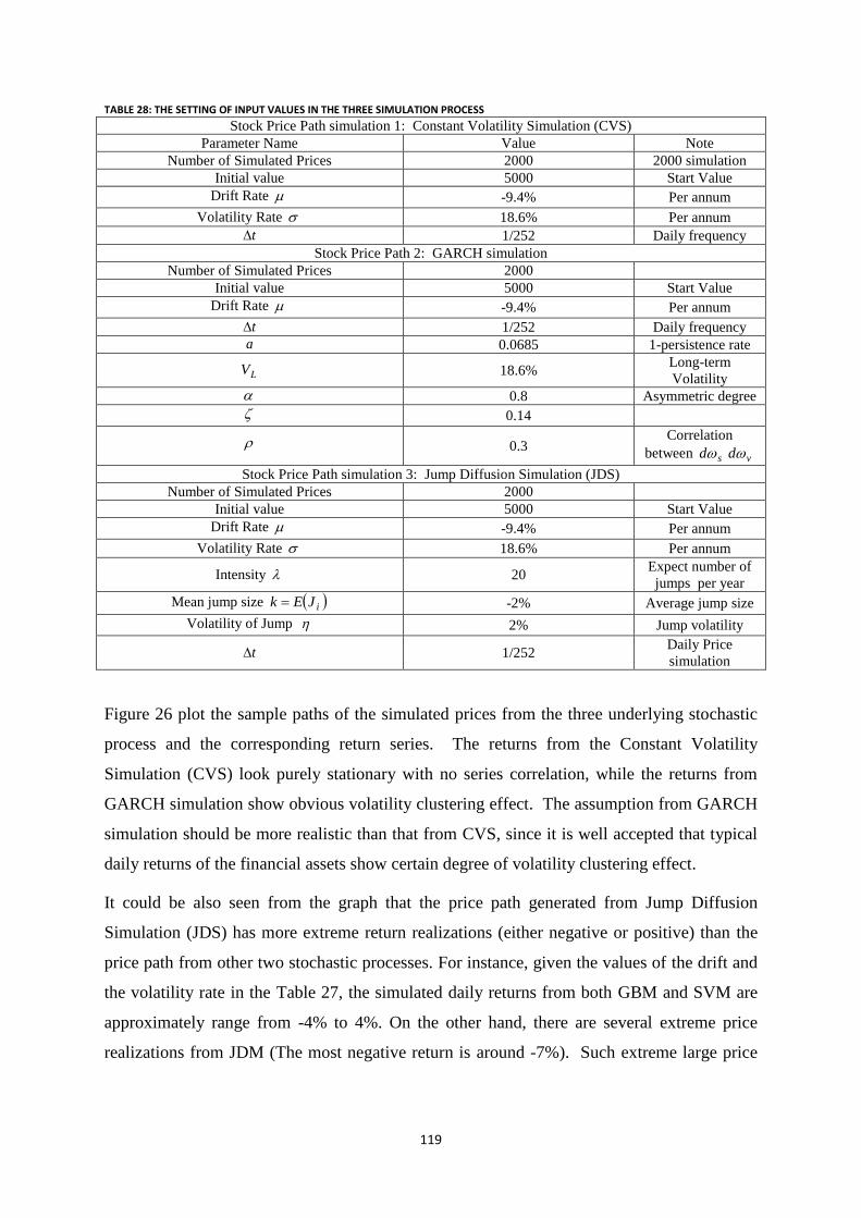
119

TABLE 28: THE SETTING OF INPUT VALUES IN THE THREE SIMULATION PROCESS

Stock Price Path simulation 1: Constant Volatility Simulation (CVS)

Parameter Name Value Note

Number of Simulated Prices 2000 2000 simulation

Initial value 5000 Start Value

Drift Rate -9.4% Per annum

Volatility Rate 18.6% Per annum

t 1/252 Daily frequency

Stock Price Path 2: GARCH simulation

Number of Simulated Prices 2000

Initial value 5000 Start Value

Drift Rate -9.4% Per annum

t 1/252 Daily frequency

a 0.0685 1-persistence rate

LV 18.6% Long-term

Volatility

0.8 Asymmetric degree

0.14

0.3 Correlation

between sd vd

Stock Price Path simulation 3: Jump Diffusion Simulation (JDS)

Number of Simulated Prices 2000

Initial value 5000 Start Value

Drift Rate -9.4% Per annum

Volatility Rate 18.6% Per annum

Intensity 20 Expect number of

jumps per year

Mean jump size iJEk -2% Average jump size

Volatility of Jump 2% Jump volatility

t 1/252 Daily Price

simulation

Figure 26 plot the sample paths of the simulated prices from the three underlying stochastic

process and the corresponding return series. The returns from the Constant Volatility

Simulation (CVS) look purely stationary with no series correlation, while the returns from

GARCH simulation show obvious volatility clustering effect. The assumption from GARCH

simulation should be more realistic than that from CVS, since it is well accepted that typical

daily returns of the financial assets show certain degree of volatility clustering effect.

It could be also seen from the graph that the price path generated from Jump Diffusion

Simulation (JDS) has more extreme return realizations (either negative or positive) than the

price path from other two stochastic processes. For instance, given the values of the drift and

the volatility rate in the Table 27, the simulated daily returns from both GBM and SVM are

approximately range from -4% to 4%. On the other hand, there are several extreme price

realizations from JDM (The most negative return is around -7%). Such extreme large price

120

movements over the short time interval almost impossible appears under the CVS or GARCH

simualtion and could only be quantified by adding jump diffusion simulation (JDS).

FIGURE 26: THE SAMPLE PATHS OF THE SIMULATED PRICES (WITH 1877 OBSERVATIONS)

0

1000

2000

3000

4000

5000

6000

7000

8000

1

13

5

26

9

40

3

53

7

67

1

80

5

93

9

10

73

1

20

7

13

41

1

47

5

16

09

1

74

3

18

77

Simulated Price

Geometric Brownian Motion

Merton Jump Diffusion Process

Stochastic Volatility Model

-0.06

-0.04

-0.02

0

0.02

0.04

0.06

1

82

16

3

24

4

32

5

40

6

48

7

56

8

64

9

73

0

81

1

89

2

97

3

10

54

11

35

12

16

12

97

13

78

14

59

15

40

16

21

17

02

17

83

18

64

19

45

Constant Volatility Simulation

Geometric Brownian Motion

-0.1

-0.05

0

0.05

0.1

1

82

16

3

24

4

32

5

40

6

48

7

56

8

64

9

73

0

81

1

89

2

97

3

10

54

11

35

12

16

12

97

13

78

14

59

15

40

16

21

17

02

17

83

18

64

19

45

Jump Diffusion Simulation

Jump Diffusion Model

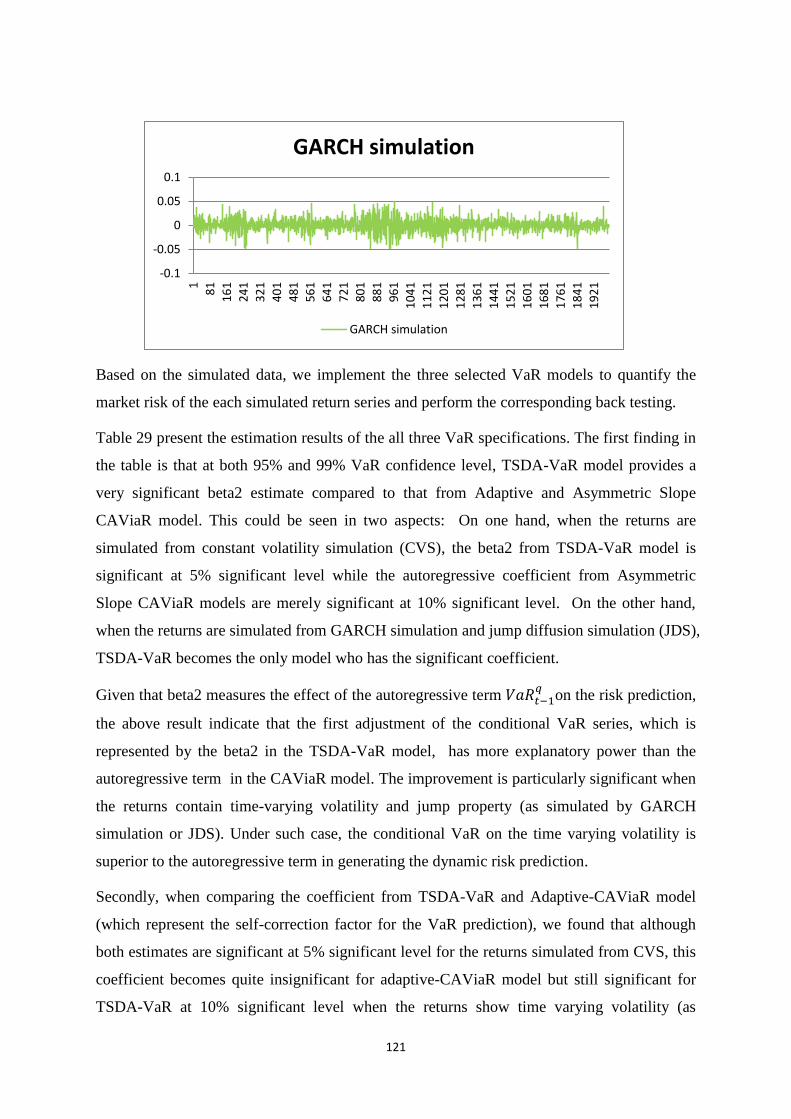
121

Based on the simulated data, we implement the three selected VaR models to quantify the

market risk of the each simulated return series and perform the corresponding back testing.

Table 29 present the estimation results of the all three VaR specifications. The first finding in

the table is that at both 95% and 99% VaR confidence level, TSDA-VaR model provides a

very significant beta2 estimate compared to that from Adaptive and Asymmetric Slope

CAViaR model. This could be seen in two aspects: On one hand, when the returns are

simulated from constant volatility simulation (CVS), the beta2 from TSDA-VaR model is

significant at 5% significant level while the autoregressive coefficient from Asymmetric

Slope CAViaR models are merely significant at 10% significant level. On the other hand,

when the returns are simulated from GARCH simulation and jump diffusion simulation (JDS),

TSDA-VaR becomes the only model who has the significant coefficient.

Given that beta2 measures the effect of the autoregressive term

on the risk prediction,

the above result indicate that the first adjustment of the conditional VaR series, which is

represented by the beta2 in the TSDA-VaR model, has more explanatory power than the

autoregressive term in the CAViaR model. The improvement is particularly significant when

the returns contain time-varying volatility and jump property (as simulated by GARCH

simulation or JDS). Under such case, the conditional VaR on the time varying volatility is

superior to the autoregressive term in generating the dynamic risk prediction.

Secondly, when comparing the coefficient from TSDA-VaR and Adaptive-CAViaR model

(which represent the self-correction factor for the VaR prediction), we found that although

both estimates are significant at 5% significant level for the returns simulated from CVS, this

coefficient becomes quite insignificant for adaptive-CAViaR model but still significant for

TSDA-VaR at 10% significant level when the returns show time varying volatility (as

-0.1

-0.05

0

0.05

0.1 1

81

16

1

24

1

32

1

40

1

48

1

56

1

64

1

72

1

80

1

88

1

96

1

10

41

11

21

12

01

12

81

13

61

14

41

15

21

16

01

16

81

17

61

18

41

19

21

GARCH simulation

GARCH simulation

122

simulated by GARCH) or jump property (as simulated by JDS). This indicated that the

modified time varying self-correction factor in TSDA-VaR model is more robust than the

static self-correction factor in Adaptive-CAViaR model in capturing the time varying risk

evolution or the unexpected shock (price jump).

Finally, the coefficient of beta4 in the TSDA-VaR model, which represents the panic selling

effect if the daily loss is greater than 2%, is significant at 10% significant level for all three

simulated return series. This confirm that adding such dummy variable into quantile

regression specification do improve the model forecast ability.

TABLE 29: QUANTILE ESTIMATION RESULT FOR THE THREE VAR MODELS FROM THE SIMULATED PRICE

VaR99% TSDA-CAVaR Adaptive-CAViaR Asymmetric Slope-CAViaR

CVS GARCH JDS CVS GARCH JDS CVS GARCH JDS

Beta1

errors

P-value

-0.053

(0.033)

0.108

0.0162

(0.0216)

0.0216

-0.115

(0.0534)

0.0310

-0.038

(0.0066)

0.0000

-0.013

(0.0059)

0.0256

-0.044

(0.010)

0.000

Beta2

errors

P-value

0.646

(0.221)

0.004

0.4228

(0.1979)

0.0398

0.7091

(0.3268)

0.0368

-0.319

(0.266)

0.0994

0.1896

(0.204)

0.1593

0.1350

(0.288)

0.6399

-0.4909

(0.407)

0.0695

0.4217

(0.4392)

0.1260

-0.284

(0.327)

0.2692

Beta3

errors

P-value

-0.008

(0.0042)

0.074

-0.058

(0.003)

0.097

-0.012

(0.004)

0.034

0.2105

(0.1267)

0.0969

-0.3797

(0.169)

0.0252

-0.022

(0.074)

0.2002

Beta4 -0.088

(0.022)

0.0122

-0.129

(0.075)

0.071

-0.1939

(0.1219)

0.0619

-0.043

(0.017)

0.0226

-0.007

(0.012)

0.2845

-0.064

(0.051)

0.206

0.0235

(0.036)

0.1176

0.2896

(0.1188)

0.0149

0.8118

(0.142)

0.0000

errors

P-value

Pseudo R^2 0.2214 0.1133 0.1349 0.2166 0.0410 0.0791 0.1697 0.1399 0.1047

VaR95% TSDA-CAVaR Adaptive-CAViaR Asymmetric Slope-CAViaR

CVS GARCH JDS CVS GARCH JDS CVS GARCH JDS

Beta1 -0.008

(0.0074)

0.068

-0.0273

(0.0203)

0.1784

-0.0333

(0.0177)

0.0601

-0.0258

(0.0091)

0.0049

-0.0259

(0.0054)

0.0000

-0.021

(0.007)

0.0058

errors

P-value

Beta2 0.2147

(0.1911)

0.0432

0.3913

(0.2011)

0.0318

0.2336

(0.1356)

0.0616

-0.297

(0.195)

0.049

-0.4236

(0.4783)

0.3281

0.2155

(0.339)

0.5256

-0.3317

(0.3761)

0.1561

0.4120

(0.4026)

0.1169

0.0967

(0.338)

0.7753

errors

P-value

Beta3 0.0168

0.0120

(0.064)

-0.0045

(0.0032)

0.0829

-0.0174

(0.0051)

0.0007

0.0313

(0.0411)

0.0992

-0.1728

(0.1024)

0.0846

-0.079

(0.069)

0.0731

errors

P-value

Beta4 -0.0139

(0.0126)

0.0840

-0.0324

(0.0309)

0.0902

-0.0344

(0.0304)

0.0775

-0.017

(0.011)

0.079

-0.0183

(0.0191)

0.23724

-0.026

(0.03)

0.205

0.0903

0.0826

0.0747

0.2758

(0.1095)

0.0119

0.0012

(0.009)

0.0692

errors

P-value

Pseudo R^2 0.202 0.1571 0.1759 0.275 0.157 0.091 0.0113 0.147 0.173 TSDA-VaR:

Adaptive-CAViaR:

Asymmetric Slope-CAViaR:

123

Similarly to what we’ve done to the historical data, two approaches are applied to quantify

the model performance, in which the back-testing models are applied in the first step for the

model validation check and the efficiency test is applied afterwards for the model accuracy

check.

The back-testing result is presented in the Table 30. The result shows that when the returns

are simulated from CVS, all three VaR models perform approximately equally well in the

failure rate, conditional coverage and DQ test. The small value of the ratio and the

ratio generated from all three VaR models indicate that the null hypothesis, which states

that model’s confidence level are correctly specified and there is no violation clustering effect

between the observation violations, are not reject. The P-values of the DQ test in all three

CAViaR could be a further evidence to support that violations are independent and non-

predictable of each other.

On the other hand, when the returns are simulated from GARCH simulation, both Adaptive

and Asymmetric Slope CAViaR models could merely pass the failure rate test but perform

badly for the conditional coverage and DQ test, especially under the 95% VaR confidence

level. The relatively large value of the Ratio and the small DQ P-values imply that we

could reject the null in the conditional coverage test that the violations are not clustering and

could not reject the null in the DQ test that the violations are correlated with their own lags

and predictable.

The TSDA-VaR model, on the other hand, could still pass all three tests with similarly

Ratio and P-value. Since the GARCH simulation could appropriately proxy the time varying

volatility of the returns contrast to the constant volatility rate in the CVS, above results

indicated that TSDA-VaR model is more adaptable than the Adaptive and Asymmetric Slope

CAViaR model to the time varying risk evolution, which is in fact the most crucial

consideration in the dynamic risk management.

Finally we turn to the result of the returns simulated from JDS. As mentioned above, Jump

Diffusion Model takes into account the effect of the random price jumps, in which the

simulated returns could undertake large unexpected movement over a short time period that

unlike happened in both CVS and GARCH simulation. From the view of the active risk

manager, such jump property is fairly desirable in describing the strong price fluctuations and

extreme market risk.

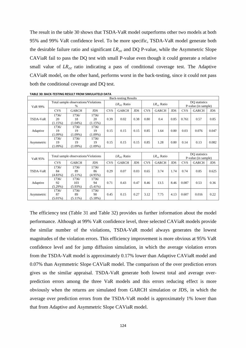
124

The result in the table 30 shows that TSDA-VaR model outperforms other two models at both

95% and 99% VaR confidence level. To be more specific, TSDA-VaR model generate both

the desirable failure ratio and significant and DQ P-value, while the Asymmetric Slope

CAViaR fail to pass the DQ test with small P-value even though it could generate a relative

small value of ratio indicating a pass of conditional coverage test. The Adaptive

CAViaR model, on the other hand, performs worst in the back-testing, since it could not pass

both the conditional coverage and DQ test.

TABLE 30: BACK-TESTING RESULT FROM SIMULATELD DATA Back-testing Results

VaR 99%

Total sample observations/Violations %

Ratio Ratio DQ statistics

P-value (in sample)

CVS GARCH JDS CVS GARCH JDS CVS GARCH JDS CVS GARCH JDS

TSDA-VaR

1736/

20 (1.15%)

1736/

18 (1.04%)

1736/

20 (1.15%)

0.39 0.02 0.38 0.80 0.4 0.85 0.761 0.57 0.85

Adaptive

1736/

19

(1.09%)

1736/

19

(1.09%)

1736/

19

(1.09%)

0.15 0.15 0.15 0.85 1.64 0.80 0.03 0.076 0.047

Asymmetric

1736/

19

(1.09%)

1736/

19

(1.09%)

1736/

19

(1.09%)

0.15 0.15 0.15 0.85 1.28 0.80 0.14 0.13 0.082

VaR 95% Total sample observations/Violations Ratio Ratio

DQ statistics

P-value (in sample)

CVS GARCH JDS CVS GARCH JDS CVS GARCH JDS CVS GARCH JDS

TSDA-VaR

1736/

84 (4.83%)

1736/

89 (5.11%)

1736/

86 (4.95%)

0.29 0.07 0.03 0.65 3.74 1.74 0.74 0.85 0.625

Adaptive

1736/

92 (5.29%)

1736/

103 (5.93%)

1736/

94 (5.41%)

0.71 0.43 0.47 8.46 13.5 8.46 0.087 0.53 0.36

Asymmetric

1736/

87

(5.01%)

1736/

89

(5.11%)

1736/

90

(5.18%)

0.45 0.15 0.27 3.12 7.75 4.13 0.607 0.016 0.22

The efficiency test (Table 31 and Table 32) provides us further information about the model

performance. Although at 99% VaR confidence level, three selected CAViaR models provide

the similar number of the violations, TSDA-VaR model always generates the lowest

magnitudes of the violation errors. This efficiency improvement is more obvious at 95% VaR

confidence level and for jump diffusion simulation, in which the average violation errors

from the TSDA-VaR model is approximately 0.17% lower than Adaptive CAViaR model and

0.07% than Asymmetric Slope CAViaR model. The comparison of the over prediction errors

gives us the similar appraisal. TSDA-VaR generate both lowest total and average over-

prediction errors among the three VaR models and this errors reducing effect is more

obviously when the returns are simulated from GARCH simulation or JDS, in which the

average over prediction errors from the TSDA-VaR model is approximately 1% lower than

that from Adaptive and Asymmetric Slope CAViaR model.

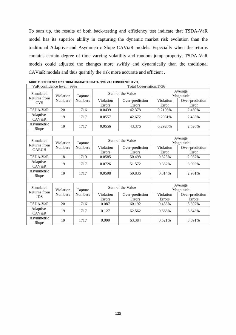
125

To sum up, the results of both back-testing and efficiency test indicate that TSDA-VaR

model has its superior ability in capturing the dynamic market risk evolution than the

traditional Adaptive and Asymmetric Slope CAViaR models. Especially when the returns

contains certain degree of time varying volatility and random jump property, TSDA-VaR

models could adjusted the changes more swiftly and dynamically than the traditional

CAViaR models and thus quantify the risk more accurate and efficient .

TABLE 31: EFFICIENCY TEST FROM SIMULATELD DATA (99% VAR CONFIDENCE LEVEL)

VaR confidence level : 99% Total Observation:1736

Simulated

Returns from

CVS

Violation

Numbers

Capture

Numbers

Sum of the Value Average

Magnitude

Violation

Errors

Over-prediction

Errors

Violation

Error

Over-prediction

Error

TSDA-VaR 20 1716 0.0439 42.378 0.2195% 2.469%

Adaptive-

CAViaR 19 1717 0.0557 42.672 0.2931% 2.485%

Asymmetric

Slope 19 1717 0.0556 43.376 0.2926% 2.526%

Simulated

Returns from

GARCH

Violation

Numbers

Capture

Numbers

Sum of the Value Average

Magnitude

Violation

Errors

Over-prediction

Errors

Violation

Error

Over-prediction

Error

TSDA-VaR 18 1719 0.0585 50.498 0.325% 2.937%

Adaptive-

CAViaR 19 1717 0.0726 51.572 0.382% 3.003%

Asymmetric

Slope 19 1717 0.0598 50.836 0.314% 2.961%

Simulated

Returns from

JDS

Violation

Numbers

Capture

Numbers

Sum of the Value Average

Magnitude

Violation

Errors

Over-prediction

Errors

Violation

Errors

Over-prediction

Errors

TSDA-VaR 20 1716 0.087 60.192 0.435% 3.507%

Adaptive-

CAViaR 19 1717 0.127 62.562 0.668% 3.643%

Asymmetric

Slope 19 1717 0.099 63.384 0.521% 3.691%

126

TABLE 32: EFFICIENCY TEST FROM SIMULATELD DATA (95% VAR CONFIDENCE LEVEL)

VaR confidence level : 95% Total Observation:1736

Simulated

Returns

from CVS

Violation

Numbers

Capture

Numbers

Sum of the Value Average

Magnitude

Violation

Errors

Over-prediction

Errors

Violation

Error

Over-prediction

Error

TSDA-VaR 84 1652 0.27216 33.419 0.324% 2.023%

Adaptive-

CAViaR 92 1644 0.36432 34.113 0.396% 2.075%

Asymmetric

Slope 87 1649 0.31233 33.540 0.359% 2.034%

Simulated

Returns

from

GARCH

Violation

Numbers

Capture

Numbers

Sum of the Value Average

Magnitude

Violation

Errors

Over-prediction

Errors

Violation

Error

Over-prediction

Error

TSDA-VaR 89 1647 0.283 39.6 0.318% 2.408%

Adaptive-

CAViaR 103 1623 0.424 52.19 0.412% 3.216%

Asymmetric

Slope 89 1647 0.299 55.59 0.322% 3.398%

Simulated

Returns

from JDS

Violation

Numbers

Capture

Numbers

Sum of the Value Average

Magnitude

Violation

Errors

Over-prediction

Errors

Violation

Errors

Over-prediction

Errors

TSDA-VaR 86 1650 0.4601 45.72 0.535% 2.771%

Adaptive-

CAViaR 94 1642 0.664392 65.10 0.7068% 3.965%

Asymmetric

Slope 90 1646 0.5409 65.37 0.601% 3.972%

4.4.4 Multiday VaR generation from TSDA-VaR model

The TSDA-VaR model proposed in this research could be adapted for the multi-horizon risk

prediction. Under the assumption that the conditional distributions of the returns are identical

and independent, the multiday variance could be estimated by integrating the daily volatility

forecast from the GARCH model. This should be a more accurate multiday variance forecast

approach than the simply the time squared root rule.

More explicitly, the VaR forecast on day using TSDA-VaR model could be

generated as follows:

1. Estimated the variances as the sum of the latest daily variances, which

are obtained from the re-estimated GARCH models at daily frequency.

127

2. Estimated the multiday VaR of residuals using historical approximation. More

explicitly, we rank the whole residual series from GARCH models in ascending order

and selected the percentage as the

3. Repeat the step 1 and 2 to generate series of and

4. Generate the dependent variable multi-period return series from sample data

5. Fit the multiday series ,

and into the following quantile

regression and generate the forecast

(4.15)

The most attractive property of the multiday VaR generate from this process is that it can

react fairly swift to the new arrived information in the returns. The users who apply this

process will generate a dynamic multi-day VaR series which compass the latest information

in the returns (step 1 and 2). These Multi-day VaR series will then be re-adjusted by the

current information using quantile regression model (4.15). This is a two-step dynamic

adjustment process, in which any time evolution of the return in the next coming day will

affect the Multi-day VaR series estimated from the first round dynamic adjustment, which in

turn, affect the quantile regression result in the second round dynamic adjustment.

4.5 Conclusion

Modeling the time varying risk evolution has always been the central consideration in the

financial risk management. Although the existing VaR models have allowed the market risk

to be appropriately captured at the certain point of time, the dynamic evolution of the return

distribution over time will possibly make the outcomes from these models unreliable. To

address this problem, this chapter proposes a two-step dynamic VaR model, which integrates

the GARCH volatility modeling and quantile regression technique. Under this process, the

time varying conditional volatility generated from the GARCH types of volatility model is

used as the explanatory variable in the time varying conditional quantile regression. Both

dynamic adjustment of the volatility and the quantile in this model enable the output VaR

128

estimate to more efficient capture the actual risk evolution in the market. Moreover, we show

how this approach could be used for the multi-period VaR prediction. The conditional

multiday distribution generated from this model is easy to implement and encompass more

information than the simple time squared root rule.

129

5. Generating volatility forecasts from ARMAX process

This chapter proposes an ARMAX model from volatility forecasts. The motivation stems

from the empirical research by Pearson and Tukey (1965), which states that for a variety of

probability distributions, there is a remarkably consistency of the ratio between volatility and

symmetric quantile interval. Taylor (2005) applied this idea by constructing volatility as a

function of symmetric quantile interval, in which the symmetric quantile are estimated by

Engle’s CAViaR model. This research specifies a new quantile regression model which has

separate forms for the left and the right quantile. Furthermore, instead of using LS regression

proposed by Taylor, an ARMAX process is proposed in this research which is motivated by

GARCH types of volatility models. This process relaxes the assumption in the Taylor’s LS

regression, in which the unobserved true variance is approximated by the realized return

square in the parameter estimation process. In fact under such assumption, the autoregressive

term of the return square should have some desirable power in explaining the time varying

volatility. The ARMAX model proposed in this paper, on the other hand, does not require

any assumption about the value of the unobserved variance. We therefore proposed it as an

appropriate model for volatility forecasts.

5.1 Introduction

Volatility forecast plays an important role in the financial risk management and asset pricing.

For instance, volatility is essentially synonymous with risk, which is crucial to the estimation

of a financial position’s Value at Risk. The famous Black-Scholes- Merton formula shows

that the price of European types of option is a function of several market variables, among

which volatility is the central consideration. Furthermore, under the mean-variance

framework of the modern portfolio theory, volatility is one of the key factors in determining

the optimal asset allocation. Recently, volatility has becomes a standard financial instrument

trading in the financial market. For instance, the implied volatility corresponding to the

S&P500 (known as VIX) has traded on traded on CBOE on March of 2004.

One property of volatility is that its true value cannot be observed directly from the financial

market, because the historical data only provide a single path of the random price evolution.

For example, daily historical prices merely contain a single data for each trading day and

therefore only reflect a sample of the overnight price changes. With increasing availability of

high frequency data such as minute or second transaction data, daily variance could be

approximated by summing up all intraday changes of the realized prices, under the

130

assumption that the price series follows random walk. However, the accuracy of such

estimate is still questionable, because the high frequency data contain fairly limited overnight

information from the closing price on t-1 day to the opening price on t day. As shown by

Rydberg and Shephard (2003), the ignorance of overnight volatility from high frequency data

will probably lead to the under-estimation the true volatility. Besides, the high frequency data

is also subjected to data collection errors.

Although volatility cannot be directly observed, it has some statistical features that can be

widely seen in the historical return series. For instance, financial asset volatility shows

obvious clustering and autocorrelation effect. Besides, volatility series are often stationary

and has seldom jumps. Finally, volatility responds differently to the large price increase and

large price decrease.

How to accurately characterize these features of the volatility have always been the central

considerations in the volatility modeling development. Generally speaking, the existing

models could be divided into three categories, which are market-based model, time series

model and quantile-based model. Market-based model backs out the implied volatility from

the market price of the corresponding option contract, under the assumption that the option’s

price is correctly determined by the Black-Scholes-Merton formula. Time series model

generates volatility forecasts by fitting the historical return series into some predetermined

time series models, in which most popular used models are GARCH class of models and

stochastic volatility models. Quantile-based approach, on the other hand, estimate volatility

from sample quantile estimates. This idea stems from the Pearson and Tukey’s research

which shows that for a variety of probability distributions, there is a remarkably consistency

of the ratio between volatility and symmetric quantile interval. Volatility is estimated as the

product of symmetric quantile interval and constant scale parameter.

This research adopts the idea of generating volatility from symmetric quantile interval.

However, instead of assuming the volatility as a uni-variable function of symmetric quantile

interval, we consider a more general ARMAX process, which is transformed from GARCH

process. The evaluation of the forecasting performance shows that volatility generated from

this process could fairly dynamically and swiftly captures the time varying market fluctuation.

The chapter is structured as follows: Section 2 provides a brief illustration of the existing

volatility models. Section 3 introduces the ARMAX process proposed in this research.

Section 4 presents the empirical analysis and some comparison between the different

131

volatility models. Sections 5 provide further extensions and implication. Sections 6 make the

conclusion.

5.2 Literature review of the volatility models

The fundamental assumption of the volatility modeling is that the financial asset returns are

not series correlated (or only low-order series correlated) but not independent. Under this

assumption, return follow a stationary ARMA process, which can be expressed as:

(5.1)

Where:

is the error terms at time

is the exogenous variable

, , are parameters to be estimated.

The choice of the lag terms largely depends on the sampling frequency of the return

series. Empirical research from Tsay (2003) shows that the daily returns of the market index

have fairly low level of series-correlation, while the monthly returns have seldom any

significant series-correlation. The choice of the exogenous variable on the other hand, is

fairly flexible. For instance, dummy variable could be introduced to represent the weekend

effect or January effect. Based on CAPM model, could be set equal to the overall market

return as well.

The error term represent the disturbance or the innovation of the return at time . This

term cannot be explained by the information up to time and is exactly the term

concerned in the volatility modeling. Denote the conditional volatility at time as:

(5.2)

The volatility modeling is essentially aim to find an appropriate model to characterize the

variance of the innovation

5.2.1 Time series volatility model

The most widely used deterministic function to depict the variance of the innovation is so

called Generalized Autoregressive Conditional Heteroskedasticity (GARCH) model, which

132

was first proposed by Bollerslev (1986). Under the standard GARCH framework, the

conditional variance is expressed as a linear function of the lagged squared innovation

terms and the lagged conditional variance terms itself. For instance, the standard GARCH (m,

j) process can be expressed as:

(5.3)

This process could appropriately capture the clustering effect in the time varying volatilities.

As long as the parameters in (5.3) satisfied the certain constraints, the excess kurtosis of the

innovation is positive, indicating that the GARCH process will generate a fatter tail

distribution than standard normal.29

One improvement of the standard GARCH is TGARCH model. This development is based on

the assumption that the conditional volatility will respond differently to the price increase and

price decrease. To be specific, Glosten, Jagannathan and Runkle (1993) proposed a

TGARCH process, which can be expressed as:

(5.4)

where the added parameter is an indicator variable corresponding to which can be

expressed as:

(5.5)

The indicator variable ensures that the model will assign a larger weight equal to

to the negative than to the positive (which is only

). The boundary

zero in the indicator function is the threshold and in more general case, this boundary could

be set equal to values other than this value.

Another GARCH types of model considering the asymmetric effect of the returns is

Exponential GARCH (EGARCH), which was developed by Nelson (1991). Instead of

treating , this model applied to

, which relax the constraint of the non-negative

predict value from the standard GARCH model. Besides, a function form of is introduced

in this model to reflect the asymmetric effect of returns, which can be expressed as:

29

See the detaied proof in Tsay (2005)

133

(5.6)

where:

(5.7)

where is the degree of freedom from student , is the Gamma function

For the selected distribution of , EGARCH process can be expressed as:

(5.8)

where is the lag operator.

To satisfy the stationary property, the roots of the Polynomials from both numerator and

denominator in the right hand side of formula (5.8) should lay outside the unit circle. More

detailed discussion of EGARCH model can be found in Nelson’ research (1991).

5.2.2 Stochastic volatility model

An alternative way to characterize the time varying volatility is to introduce a random process

for the conditional variance. This model was developed by Harvey, Ruiz and Shephard

(1994). Similar to EGARCH model, Stochastic Volatility model (SV) applies directly to

to ensure that the conditional variance prediction is non-negative.

Consider the following stochastic volatility model:

(5.9)

Under the model assumption, both and are i.i.d. series

and , are independent of each other

Although the introduction of the random variable largely increased the model’s flexibility,

the parameter estimation procedure also becomes complex, which involves applying Quasi-

likelihood estimation approach through Kalman filter or Markov Chain Monte Carlo

simulation (MCMC). Empirical research from Jacquier, Polson and Rossi (1994) shows that

134

although the SV types of model improve the model’s fitness to the actual data, it provide no

significant improvement of the out-sample forecast accuracy than other types of volatility

models.

5.2.3 Extracting volatility from symmetric quantile interval

The idea of estimating volatility from symmetric quantile interval is originally proposed by

Pearson and Tukey (1965). They show from their research that for large number of

probability distributions, there is a remarkably constancy of the ratio between the volatility

and the symmetric quantile interval. For instance, they provide the following simple

approximations of volatility using symmetric quantile interval as:

Taylor (2005) utilized the idea by constructing a Least Square regression for the variance

prediction, which is expressed in following form:

(5.10)

The symmetric quantile forecast and are estimated from the quantile

regression model (CAViaR) proposed by Engle and Manganelli (2004).

Volatility prediction could be generated using model (5.10) after corresponding parameters

been estimated. Taylor shows that compared to GARCH models, this approach requires no

parametric assumption on the conditional distribution, and therefore it should capture the

time varying volatility better than GARCH models if the left and the right tails of the

conditional distribution are driven by different forces over time.

5.3 Volatility modeling using ARMAX process

Given that the quantile estimated from the CAViaR models have been commonly used in the

risk management for assessing the financial asset’s Value at Risk, Taylor’s approach provide

an innovated idea of how to integrate parametric time-series model and quantitative risk

measurement into volatility forecast.

Since the true volatility is unobservable, this idea provides us a new way to improve the

accuracy of the volatility forecast. That is, if we could improve the accuracy of the symmetric

quantile estimates, the accuracy of the corresponding volatility forecast should also be

increased as well.

135

In order to improve the accuracy of the symmetric quantile estimates, we proposed a new

quantile regression model in this research. To be specific, instead of using Engel’s CAViaR

as proposed in Taylor’s research, we apply the following quantile regression model:

(5.11)

where:

is the implied volatility of the corresponding asset observed in the market at time

is an indicator variable related to the actual return at time , which is expressed

as:

(5.12)

There are two changes of this quantile regression model compared to CAViaR model. Firstly,

the model replace the auto-regressive term in CAViaR model by the implied

volatility . Compared to whose value is estimated from the historical

simulation, have forward-looking property since its value is backed out from the

corresponding option matured in the future. Therefore it should respond relative swift to the

new arrived information.

Besides, we introduce an indicator variable for the symmetric quantile estimates. The

top equation of (5.12) is used for the left quantile estimate and the bottom one is used for the

right quantile estimate. This specification separates the asymmetric effect of the returns for

the left and the right Quantile. Given that the long position and the short position have a

different risk attitudes, the specification ensure that the left quantile estimate which used to

quantify the long position’s risk will assign more weight on the price decrease (the negative

returns), while the right quantile estimate which used to quantify the short position’s risk will

place more weight on the price increase (the positive return).

After obtaining the symmetric quantile estimates using model (5.12), a relationship between

the volatility and the symmetric quantile interval need to be specified. According to Taylor’s

research, a Least Square regression is introduced which can be expressed as:

(5.13)

136

However, the above regression is theoretically un-estimable because the true value of on

the right hand side of the regression is unobservable. For this reason, Taylor use the realized

return square on the time as the proxy of

. But in this research, we wish to

relax this assumption. It is intuitively to think that under the Taylor’s assumption that the true

variance could be approximated by the realized return square, the autoregressive term of the

returns square should have some desirable power in predicting the variance. This is exactly

how the GARCH model comes out. Tsay (2005) shows how to transfer a GARCH process

into a pure ARMA process of return squares. Recall the standard GARCH (1, 1) model,

which is expressed as:

(5.14)

Let

, Tsay proved that is a Martingale difference sequence (MDS)

Substituting

and

, the GARCH process (5.14) is therefore

transferred into a ARMA process of , which is expressed as:

(5.15)

Motivated by this idea, this research modify the over transfer by adding the symmetric

quantile interval in it. To see this, we replace by symmetric quantile interval

while keeping

unchanged. The GARCH process

(5.14) could be transferred into following process.

(5.16)

where

Regression (5.16) is an auto-regressive time series model with an exogenous variable, which

is proposed in this research. The parameters of this ARMAX process could be estimated by a

two-step estimation approach similarly to GARCH model. Firstly, we can re-estimate the

quantile regression model based on the pre-specified moving window data and provide one

step-ahead forecast of the symmetric quantile series. Secondly, we treat the symmetric

quantile interval

as exogenous variable and apply maximum

likelihood (ML) approach to estimate the parameters in the regression (5.16). The statistical

137

properties of the ML estimators under the MDS errors have not been rigorously studied.

However, empirical research have found that when the sample size is large and under some

basic conditions, the ML estimators are normally consistent with a high optimal convergence

rate. (see, e.g., Guido, 2000; Guoliang and Luqin, 2007)

Under the normality assumption of , the likelihood function of the regression (5.16) is

derived as:

(5.17)

where:

is the parameter vector to be estimated

is the information set on time

is the joint probability density function of to

When the sample size is largely enough, could be removed from the

likelihood function (5.17) so that the conditional log-likelihood function becomes to:

(5.18)

where could be calculated recursively by

(5.19)

In more general case, could be assumed following some more flexible distributions such as

student or General Error Distribution (GED) and the conditional likelihood function could

be derived in the similar way.

138

Taking expectation operator to both side of the regression (5.16), the volatility forecast using

ARMAX model is equal to:

(5.20)

This approach can be assumed as a refinement of the GARCH volatility using quantile

Regression technique. Because under the GARCH framework, the values of the lagged

conditional variance term is calculated by recursively using the pre-specified time series

model after setting the initial variance equal to the current return square30

. Under this

approach, however, the values of the lagged conditional variance term are directly replaced

by the symmetric quantile interval (5.19) estimated from the pre-specified quantile regression

model. The different specifications for the left and the right quantile in our quantile

regression model (5.11) further ensure that the leverage effect of the returns have been taken

into account. Although the ARMAX regression proposed in this research is straightforward,

it could possibly encompass the volatility features contained in some complex GARCH

specification due to the exogenous variable

. Besides, since the

symmetric quantile intervals are updated by the quantile regression model, the volatility

forecast from this process should fairly accurate and swiftly capture the time varying risk

evolution.

5.4 Data and empirical results

5.4.1 Estimate the symmetric quantile

To implement this approach, we use the daily data of FTSE 100 index and its corresponding

European-type options listed on LIFFE, spanning from 18 Nov 2001to 15 Nov 2010. Based

on the overall 2572 historical returns and the implied volatility observations, we fix the

moving data window of four year (1008) to estimate the parameters in the quantile regression

model (5.11). More explicitly, we estimate the left and right quantile separately using model

(5.11), which is:

(5.21)

30

See explicate derivation in Hull(2008)

139

These two models have the similar property as the Engle’ Asymmetric Slope CAViaR model

and since the observations are less than 5000 and number of the parameters to be estimated is

only four, we estimate the parameters using Simplex Algorithm proposed by Koenker and

d’Orey (1993).

To implement the optimization procedure, we generate vectors of parameters from uniform

random generator as pivotal vectors and then evaluated the Regression quantile (RQ) function.

For the vectors of the parameters which produced lowest RQ, we selected them as the

initial values and ran the Simplex Algorithm and choose the new optimal parameter vectors

as the new initial conditions for iteration. Repeating this procedure until the convergence

criterion is satisfied and we selected the parameter vector as the final optimal one. The value

of n and m is set similar to the Engel and Manganelli (2004).

Table 33 lists the least absolute deviation estimates and relevant statistics for the quantile

regression model (5.21), based on four year data from 1811/2001 to 18/11/2004. Several

points are necessary to be mentioned in this table: Firstly, the coefficient of the implied

volatility is always very significant for all three selected quantile levels, which confirms the

implied volatility have appealing predicting power in the specified quantile regression.

Secondly, is fairly significant when the quantile level is close to the tail area ( =2.5% or

5%) and becomes insignificant as the quantile level moves towards the central area ( = 10%).

This implies that the asymmetric effect is more sensitive to the extreme fluctuation than the

normal fluctuation of returns. Besides, the value of for the left and the right quantile are

significant different from each other, indicating the separation of this impact do exists in the

left and right quantile.

To generate the symmetric quantile series, we shift the 4 year data window at daily frequency

and for each set of the window data, we generate one step-ahead symmetric quantile forecast

based on the estimated quantile regression model (5.21). The whole forecasted symmetric

quantile series contain 1972 estimates staring from 19/11/2004 to 16/11/2010. In order to find

the most accurate quantile estimate from our pre-specified model, we generate three

symmetric quantile series using above procedure at quantile level , and

seperately. The accuracy of these three forecast series are checked by two back-

testing approaches, which are failure-rate test and Dynamic quantile test. This could be done

by comparing the forecasted quantile series with the actual returns over the same period from

19/11/2004 to 16/11/2010.

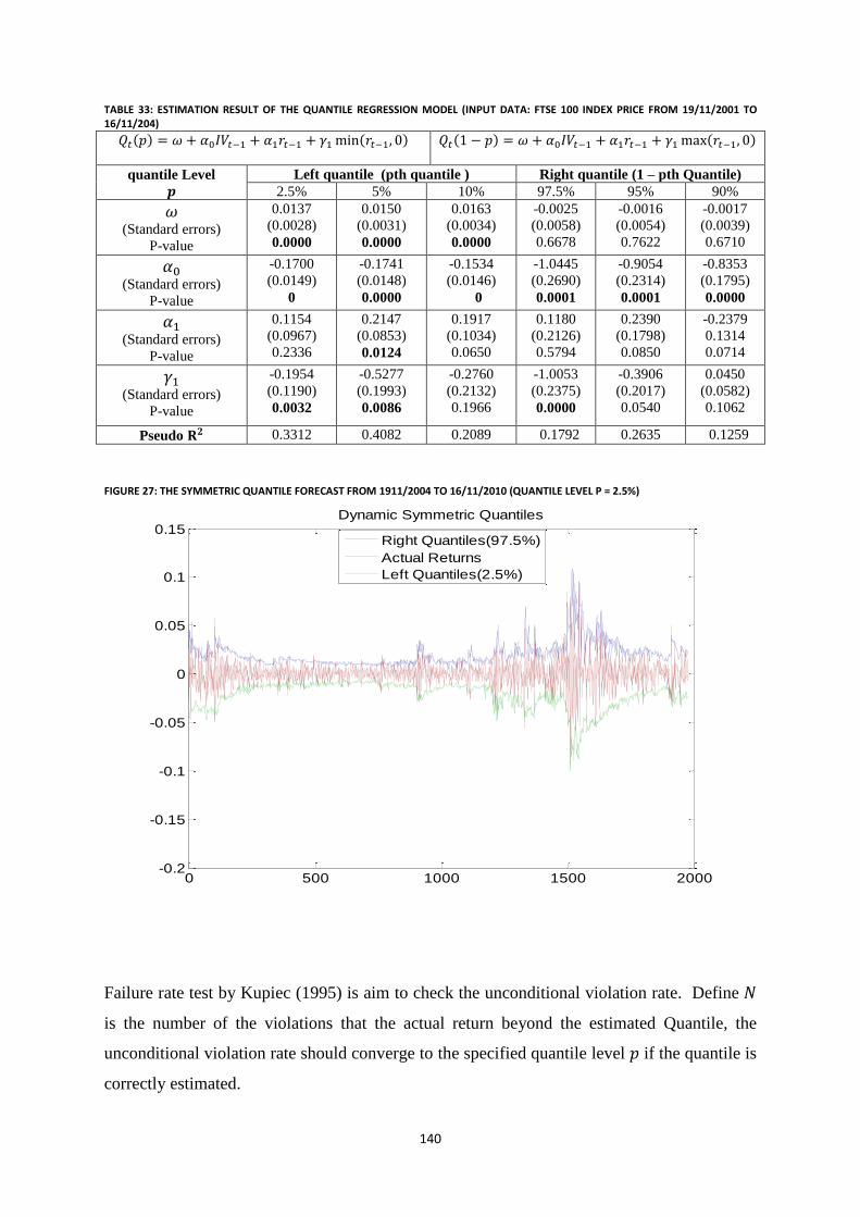
140

TABLE 33: ESTIMATION RESULT OF THE QUANTILE REGRESSION MODEL (INPUT DATA: FTSE 100 INDEX PRICE FROM 19/11/2001 TO 16/11/204)

quantile Level

Left quantile (pth quantile ) Right quantile (1 – pth Quantile)

2.5% 5% 10% 97.5% 95% 90%

(Standard errors)

P-value

0.0137

(0.0028)

0.0000

0.0150

(0.0031)

0.0000

0.0163

(0.0034)

0.0000

-0.0025

(0.0058)

0.6678

-0.0016

(0.0054)

0.7622

-0.0017

(0.0039)

0.6710

(Standard errors)

P-value

-0.1700

(0.0149)

0

-0.1741

(0.0148)

0.0000

-0.1534

(0.0146)

0

-1.0445

(0.2690)

0.0001

-0.9054

(0.2314)

0.0001

-0.8353

(0.1795)

0.0000

(Standard errors)

P-value

0.1154

(0.0967)

0.2336

0.2147

(0.0853)

0.0124

0.1917

(0.1034)

0.0650

0.1180

(0.2126)

0.5794

0.2390

(0.1798)

0.0850

-0.2379

0.1314

0.0714

(Standard errors)

P-value

-0.1954

(0.1190)

0.0032

-0.5277

(0.1993)

0.0086

-0.2760

(0.2132)

0.1966

-1.0053

(0.2375)

0.0000

-0.3906

(0.2017)

0.0540

0.0450

(0.0582)

0.1062

Pseudo 0.3312 0.4082 0.2089 0.1792 0.2635 0.1259

FIGURE 27: THE SYMMETRIC QUANTILE FORECAST FROM 1911/2004 TO 16/11/2010 (QUANTILE LEVEL P = 2.5%)

Failure rate test by Kupiec (1995) is aim to check the unconditional violation rate. Define

is the number of the violations that the actual return beyond the estimated Quantile, the

unconditional violation rate should converge to the specified quantile level if the quantile is

correctly estimated.

0 500 1000 1500 2000-0.2

-0.15

-0.1

-0.05

0

0.05

0.1

0.15Dynamic Symmetric Quantiles

Right Quantiles(97.5%)

Actual Returns

Left Quantiles(2.5%)

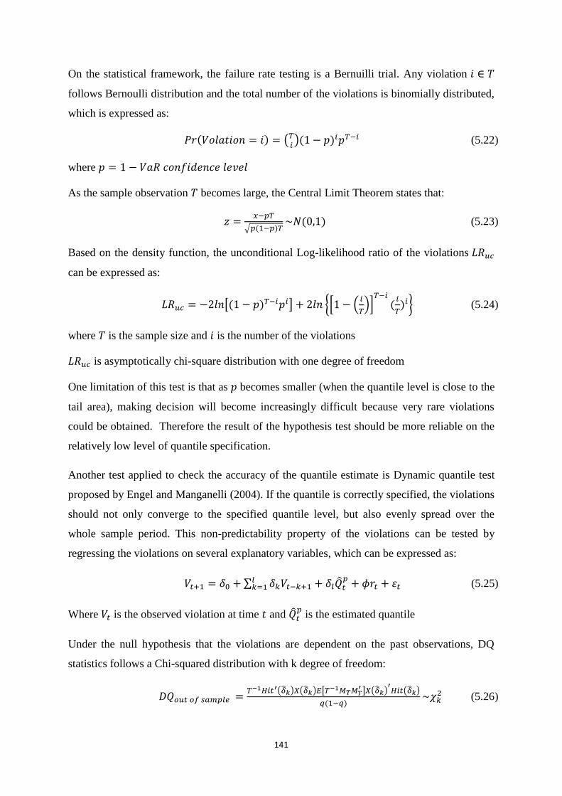
141

On the statistical framework, the failure rate testing is a Bernuilli trial. Any violation

follows Bernoulli distribution and the total number of the violations is binomially distributed,

which is expressed as:

(5.22)

where

As the sample observation becomes large, the Central Limit Theorem states that:

(5.23)

Based on the density function, the unconditional Log-likelihood ratio of the violations

can be expressed as:

(5.24)

where is the sample size and is the number of the violations

is asymptotically chi-square distribution with one degree of freedom

One limitation of this test is that as becomes smaller (when the quantile level is close to the

tail area), making decision will become increasingly difficult because very rare violations

could be obtained. Therefore the result of the hypothesis test should be more reliable on the

relatively low level of quantile specification.

Another test applied to check the accuracy of the quantile estimate is Dynamic quantile test

proposed by Engel and Manganelli (2004). If the quantile is correctly specified, the violations

should not only converge to the specified quantile level, but also evenly spread over the

whole sample period. This non-predictability property of the violations can be tested by

regressing the violations on several explanatory variables, which can be expressed as:

(5.25)

Where is the observed violation at time and is the estimated quantile

Under the null hypothesis that the violations are dependent on the past observations, DQ

statistics follows a Chi-squared distribution with k degree of freedom:

(5.26)

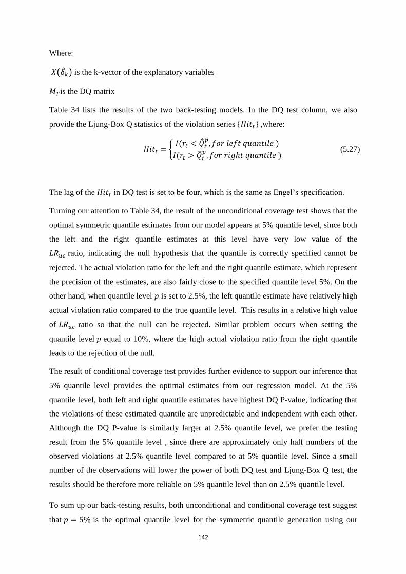
142

Where:

is the k-vector of the explanatory variables

is the DQ matrix

Table 34 lists the results of the two back-testing models. In the DQ test column, we also

provide the Ljung-Box Q statistics of the violation series ,where:

(5.27)

The lag of the in DQ test is set to be four, which is the same as Engel’s specification.

Turning our attention to Table 34, the result of the unconditional coverage test shows that the

optimal symmetric quantile estimates from our model appears at 5% quantile level, since both

the left and the right quantile estimates at this level have very low value of the

ratio, indicating the null hypothesis that the quantile is correctly specified cannot be

rejected. The actual violation ratio for the left and the right quantile estimate, which represent

the precision of the estimates, are also fairly close to the specified quantile level 5%. On the

other hand, when quantile level is set to 2.5%, the left quantile estimate have relatively high

actual violation ratio compared to the true quantile level. This results in a relative high value

of ratio so that the null can be rejected. Similar problem occurs when setting the

quantile level equal to 10%, where the high actual violation ratio from the right quantile

leads to the rejection of the null.

The result of conditional coverage test provides further evidence to support our inference that

5% quantile level provides the optimal estimates from our regression model. At the 5%

quantile level, both left and right quantile estimates have highest DQ P-value, indicating that

the violations of these estimated quantile are unpredictable and independent with each other.

Although the DQ P-value is similarly larger at 2.5% quantile level, we prefer the testing

result from the 5% quantile level , since there are approximately only half numbers of the

observed violations at 2.5% quantile level compared to at 5% quantile level. Since a small

number of the observations will lower the power of both DQ test and Ljung-Box Q test, the

results should be therefore more reliable on 5% quantile level than on 2.5% quantile level.

To sum up our back-testing results, both unconditional and conditional coverage test suggest

that is the optimal quantile level for the symmetric quantile generation using our

143

regression model (5.21). We therefore construct the dynamic symmetric quantile intervals

based on this quantile level, as shown in the Figure 28. (Symmetric quantile intervals are

plotted in the second axis, which is calculated as the difference between right and left

quantile)

TABLE 34: BACK-TESTING RESULT OF THE SYMMETRIC QUANTILE ESTIMATE AT SELECTED THREE QUANTILE LEVEL

Unconditional coverage test

Sample

Observations

Left quantile Estimates Right quantile Estimates

quantile Level Violation

Ratio quantile Level

Violation

Ratio

Left

Quantile

Right

quantile

1972

P = 2.5% 67/3.4% 1-P = 97.5% 63/3.19% 5.87 3.59

P = 5% 107/5.43% 1-P = 95% 113/5.73% 0.73 2.609

P = 10% 204/10.34% 1-P = 90% 226/11.46% 0.257 4.485

Conditional coverage test for left quantile

Left Quantile Ljung-Box tests- Q statistics P-value DQ statistics

P-value quantile Level Violations 5lags 10 lags 20lags p = 2.5% 67 0.000 0.000 0.000 0.16

p = 5% 107 0.005 0.000 0.000 0.86

p= 10% 204 0.002 0.001 0.004 0.35

Conditional coverage test for right quantile

Right Quantile Ljung-Box tests- Q statistics DQ statistics

P-value quantile Level Violations 5lags 10 lags 20lags 1-p = 97.5% 63 0.0003 0.0034 0.0050 0.28

1-p = 95% 113 0.0418 0.0262 0.0272 0.58

1-p = 90% 226 0.149 0.145 0.2614 0.14

FIGURE 28: THE DYNAMIC SYMMETRIC QUANTILE INTERVALS AT QUANTILE LEVEL P= 5%

0

0.02

0.04

0.06

0.08

0.1

0.12

0.14

0.16

0.18

0.2

-0.15

-0.1

-0.05

0

0.05

0.1

0.15

1

65

1

29

1

93

2

57

3

21

3

85

4

49

5

13

5

77

6

41

7

05

7

69

8

33

8

97

9

61

1

02

5

10

89

1

15

3

12

17

1

28

1

13

45

1

40

9

14

73

1

53

7

16

01

1

66

5

17

29

1

79

3

18

57

1

92

1

Dynamic Symmtric Quantile Intervals

Actual returns Left Quantiles Right Quantiles Symmetric Quantiles Interval

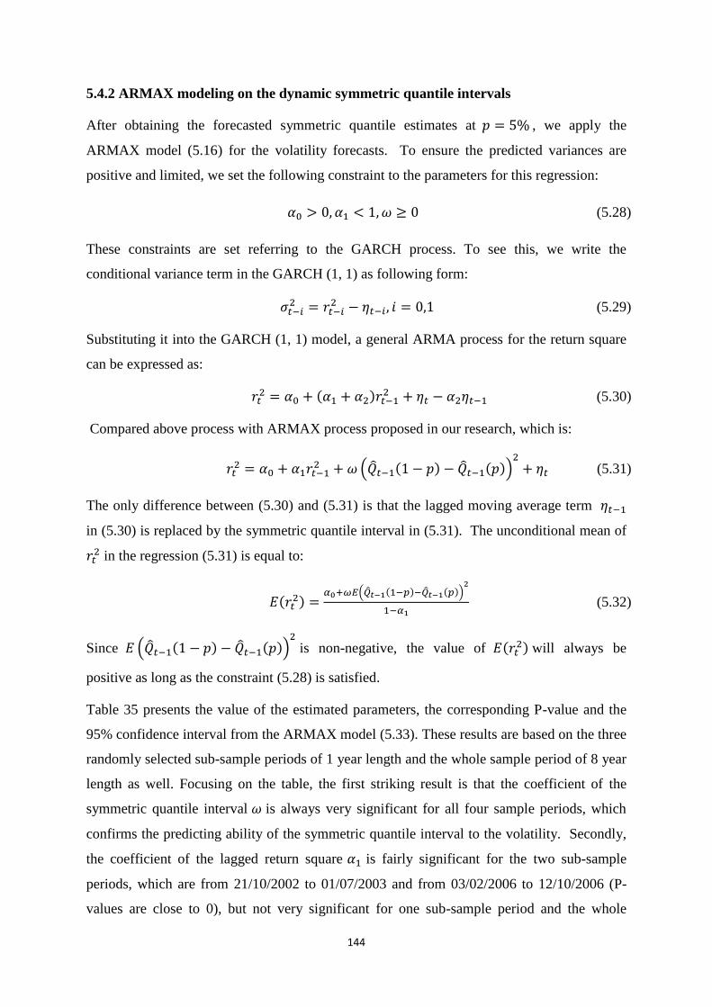
144

5.4.2 ARMAX modeling on the dynamic symmetric quantile intervals

After obtaining the forecasted symmetric quantile estimates at , we apply the

ARMAX model (5.16) for the volatility forecasts. To ensure the predicted variances are

positive and limited, we set the following constraint to the parameters for this regression:

(5.28)

These constraints are set referring to the GARCH process. To see this, we write the

conditional variance term in the GARCH (1, 1) as following form:

(5.29)

Substituting it into the GARCH (1, 1) model, a general ARMA process for the return square

can be expressed as:

(5.30)

Compared above process with ARMAX process proposed in our research, which is:

(5.31)

The only difference between (5.30) and (5.31) is that the lagged moving average term

in (5.30) is replaced by the symmetric quantile interval in (5.31). The unconditional mean of

in the regression (5.31) is equal to:

(5.32)

Since

is non-negative, the value of will always be

positive as long as the constraint (5.28) is satisfied.

Table 35 presents the value of the estimated parameters, the corresponding P-value and the

95% confidence interval from the ARMAX model (5.33). These results are based on the three

randomly selected sub-sample periods of 1 year length and the whole sample period of 8 year

length as well. Focusing on the table, the first striking result is that the coefficient of the

symmetric quantile interval is always very significant for all four sample periods, which

confirms the predicting ability of the symmetric quantile interval to the volatility. Secondly,

the coefficient of the lagged return square is fairly significant for the two sub-sample

periods, which are from 21/10/2002 to 01/07/2003 and from 03/02/2006 to 12/10/2006 (P-

values are close to 0), but not very significant for one sub-sample period and the whole

145

sample period, which are from 21/09/2004 to 30/05/2005 and 21/10/2002 to 10/08/2010 (P-

values are greater than 5% but less than 10%). This indicates that the autoregressive term of

the return square generally has a good explanatory power to the future volatility but this

relationship might not be strong and stable for any time periods. Finally, the coefficient of

the constant term is always very insignificant for all sample periods. This proves that there

is no determinist drift term contained in the time-varying volatility evolution, which is

consistent with the empirical finding by Bollerslev and Chou (1992).

TABLE 35: PARAMETER ESTIMATION OF ARMAX MODEL UNDER THREE SELECTED SAMPLE PERIODS

ARMAX regression: ttttt pQpQrr

2

112

1102 )(ˆ)1(ˆ

Maximum Log Likelihood Value:

1671.714

Sub-Sample: 21Oct2002-01Jul2003

Number of Observations:252

Parameters Coef. Std.Err. P-value [95% Confidence Interval]

0 4.29e-06 0.00011 0.969 [-0.0002 0.0002]

1 0.304141 0.02562 0.000 [0.2579 0.3583]

0.065624 0.02267 0.004 [0.0212 0.1101]

Maximum Log Likelihood Value:

1866.188

Sub-Sample: 21Sep2004 – 30May2005

Number of Observations:252

Parameters Coef. Std.Err. P-value [95% Confidence Interval]

0 7.51e-06 0.00002 0.758 [-.00004 .000055]

1 0.09031 0.03343 0.07 [.024779 .155840]

0.05274 0.00536 0.000 [.042219 .063265]

Maximum Log Likelihood Value:

1820.051

Sub-Sample: 03Feb2006 – 12Oct2006

Number of Observations:252

Parameters Coef. Std.Err. P-value [95% Confidence Interval]

0 -.0000159 .0000316 0.614 [-.0000778 .000046]

1 .2257427 .0347325 0.000 [.1576684 .2938171]

.0862907 .0058552 0.000 [.0748147 .0977666]

Maximum Log Likelihood Value:

10953.65

Whole sample: 21Oct2002-10Aug2010

Number of Observations:1972

Parameters Coef. Std.Err. P-value [95% Confidence Interval]

0 3.69e-06 .0000262 0.888 [-.0000478 .0000551]

1 .0110164 .0065596 0.093 [-.0018403 .023873]

.0656684 .0013903 0.000 [.0629435 .0683933]

To construct the dynamic volatility forecast series, we use one year data in the sample for the

parameters estimation of the ARMAX model. For each set of the parameters, one step-ahead

volatility forecast is calculated. Shifting data window at daily frequency and repeating this

procedure we could obtain overall 1720 out of sample volatility forecasts, spanning from

22/10/2002 to 11/08/2010, as plotted in the Figure 29. The red line represents the one step-

146

ahead volatility forecast series based on the ARMAX process we specified. The blue line

plotted on the secondary axis, on the other hand, represents the realized returns on the next

day.

FIGURE 29: DAILY VOLATILITY FORECASTS OF FTSE 100 INDEX FROM ARMAX PROCESS, SPANNING FROM 22/10/2002 TO 11/08/2010

To evaluate the model performance, we extract the standardized return series by dividing the

actual returns by the forecasted volatility. If the model has a high goodness of fit, the

standardized return series

should be fairly close to a white noise process.

Figure 30 plots the standardized return series against the volatility forecast series. Compared

to the original return series, the standardized series shows significant homoscedasticity with

seldom extreme outliers. Although the kernel density of the original return is deviated far

from normal distribution, the standardized returns’ density largely converge to normal. The

ACF and PACF plot in the Figure 32 also indicates that there is no strong auto-correlation

between any lag of the standardized returns from 1 to 40.

We apply Ljung-Box Q test to the standardized return series and the results shows that

)1645.0(039.26)20( Q and )3756.0(209.42)40( Q . The value in the bracket is the

0

0.01

0.02

0.03

0.04

0.05

0.06

0.07

0.08

-1.50E-01

-1.00E-01

-5.00E-02

0.00E+00

5.00E-02

1.00E-01

1.50E-01

1

61

12

1

18

1

24

1

30

1

36

1

42

1

48

1

54

1

60

1

66

1

72

1

78

1

84

1

90

1

96

1

10

21

10

81

11

41

12

01

12

61

13

21

13

81

14

41

15

01

15

61

16

21

16

81

One step-ahead Volatility Forecast

Actual Returns Volatility forecast from ARMAX

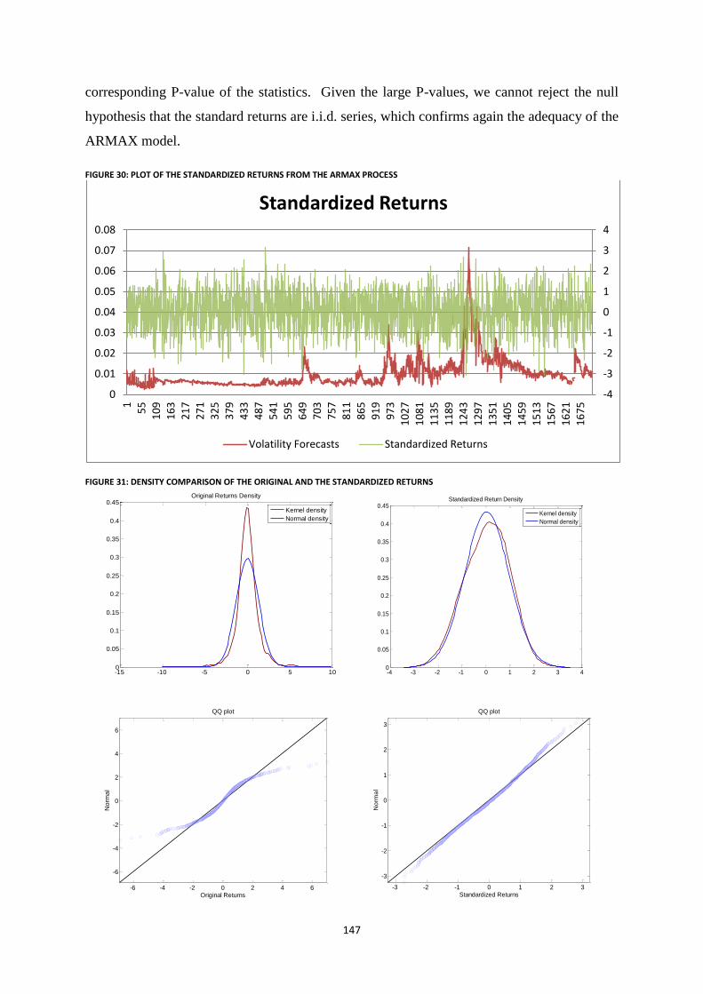
147

corresponding P-value of the statistics. Given the large P-values, we cannot reject the null

hypothesis that the standard returns are i.i.d. series, which confirms again the adequacy of the

ARMAX model.

FIGURE 30: PLOT OF THE STANDARDIZED RETURNS FROM THE ARMAX PROCESS

FIGURE 31: DENSITY COMPARISON OF THE ORIGINAL AND THE STANDARDIZED RETURNS

-4

-3

-2

-1

0

1

2

3

4

0

0.01

0.02

0.03

0.04

0.05

0.06

0.07

0.08

1

55

1

09

1

63

2

17

2

71

3

25

3

79

4

33

4

87

5

41

5

95

6

49

7

03

7

57

8

11

8

65

9

19

9

73

1

02

7

10

81

1

13

5

11

89

1

24

3

12

97

1

35

1

14

05

1

45

9

15

13

1

56

7

16

21

1

67

5

Standardized Returns

Volatility Forecasts Standardized Returns

-15 -10 -5 0 5 100

0.05

0.1

0.15

0.2

0.25

0.3

0.35

0.4

0.45Original Returns Density

Kernel density

Normal density

-4 -3 -2 -1 0 1 2 3 40

0.05

0.1

0.15

0.2

0.25

0.3

0.35

0.4

0.45Standardized Return Density

Kernel density

Normal density

-6 -4 -2 0 2 4 6

-6

-4

-2

0

2

4

6

Original Returns

No

rma

l

QQ plot

-3 -2 -1 0 1 2 3

-3

-2

-1

0

1

2

3

Standardized Returns

No

rma

l

QQ plot

148

FIGURE 32: ACF AND PACF OF THE STANDARDIZED RETURNS

5.4.3 Empirical comparison of the different volatility forecast approaches

For comparison purpose, the research also produced the dynamic volatility forecast series

from other two types of commonly used volatility models, which are EWMA volatility and

TGARCH volatility. To be specific, the EWMA volatility forecasts are generated by

following process:

(5.33)

The value of the delay factor is set equal to 0.96 according to the Riskmetric’s specification

for the daily return series. The initial value of the conditional variance is set equal to the

unconditional variance of the most recently 252 return observations during 22/10/2002 to

01/07/03.

To consider the leverage effect of the returns, we also fit the returns into following TGARCH

(1, 1) model:

(5.34)

where follows the General Error Distribution with following form:

(5.35)

-0.0

4-0

.02

0.0

00.0

20.0

40.0

6

Auto

corr

ela

tions o

f var1

3

0 10 20 30 40Lag

Bartlett's formula for MA(q) 95% confidence bands

ACF of the Standardized Returns

-0.0

50.0

00.0

5

Part

ial auto

corr

ela

tions o

f var1

4

0 10 20 30 40Lag

95% Confidence bands [se = 1/sqrt(n)]

PACF of Standardized Returns

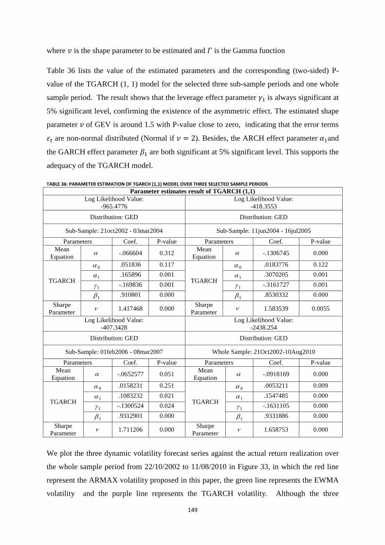
149

where is the shape parameter to be estimated and is the Gamma function

Table 36 lists the value of the estimated parameters and the corresponding (two-sided) P-

value of the TGARCH (1, 1) model for the selected three sub-sample periods and one whole

sample period. The result shows that the leverage effect parameter is always significant at

5% significant level, confirming the existence of the asymmetric effect. The estimated shape

parameter of GEV is around 1.5 with P-value close to zero, indicating that the error terms

are non-normal distributed (Normal if ). Besides, the ARCH effect parameter and

the GARCH effect parameter are both significant at 5% significant level. This supports the

adequacy of the TGARCH model.

TABLE 36: PARAMETER ESTIMATION OF TGARCH (1,1) MODEL OVER THREE SELECTED SAMPLE PERIODS

Parameter estimates result of TGARCH (1,1)

Log Likelihood Value:

-965.4776

Log Likelihood Value:

-418.3553

Distribution: GED Distribution: GED

Sub-Sample: 21oct2002 - 03mar2004 Sub-Sample: 11jun2004 - 16jul2005

Parameters Coef. P-value Parameters Coef. P-value

Mean

Equation -.066604 0.312

Mean

Equation -.1306745 0.000

TGARCH

0 .051836 0.117

TGARCH

0 .0183776 0.122

1 .165896 0.001 1 .3070205 0.001

1 -.169836 0.001 1 -.3161727 0.001

1 .910801 0.000 1 .8530332 0.000

Sharpe

Parameter 1.417468 0.000

Sharpe

Parameter 1.583539 0.0055

Log Likelihood Value:

-407.3428

Log Likelihood Value:

-2438.254

Distribution: GED Distribution: GED

Sub-Sample: 01feb2006 - 08mar2007 Whole Sample: 21Oct2002-10Aug2010

Parameters Coef. P-value Parameters Coef. P-value

Mean

Equation -.0652577 0.051

Mean

Equation -.0918169 0.000

TGARCH

0 .0158231 0.251

TGARCH

0 .0053211 0.009

1 .1083232 0.021 1 .1547485 0.000

1 -.1300524 0.024 1 -.1631105 0.000

1 .9312901 0.000 1 .9331886 0.000

Sharpe

Parameter 1.711206 0.000

Sharpe

Parameter 1.658753 0.000

We plot the three dynamic volatility forecast series against the actual return realization over

the whole sample period from 22/10/2002 to 11/08/2010 in Figure 33, in which the red line

represent the ARMAX volatility proposed in this paper, the green line represents the EWMA

volatility and the purple line represents the TGARCH volatility. Although the three

150

volatility forecast series shown in the figure have the similar trend, the ARMAX volatility

appears more flutter points than both EWMA and TGARCH volatility.

FIGURE 33: COMPARISON BETWEEN THREE VOLATILITY FORECAST SERIES. RED LINE: ARMAX VOLATILITY. GREEN LINE: EWMA VOLATILITY. PURPLE LINE: TGARCH VOLATILITY

-0.100

-0.080

-0.060

-0.040

-0.020

0.000

0.020

0.040

0.060

0.080

0.100

1

55

10

9

16

3

21

7

27

1

32

5

37

9

43

3

48

7

54

1

59

5

64

9

70

3

75

7

81

1

86

5

91

9

97

3

10

27

10

81

11

35

11

89

12

43

12

97

13

51

14

05

14

59

15

13

15

67

16

21

16

75

Comparison of Volatility Forecast Series

Actual Returns Dynamic Quantiles Volatility

EWMA Volatility TGARCH Volatility

1

2

3

4

0200

400600

8001000

12001400

16001800

0

0.01

0.02

0.03

0.04

0.05

0.06

0.07

Comparison of Volatility Forecast Series

Dynamic Quantile Volatility

EWMA Volatility

TGARCH Volatility

Implied Volatility

151

Due to the Non-observability of the true volatility, it is statistically difficult to compare the

forecast performance of different types of volatility models. One feasible evaluation

approach in the literature is to compare the out of sample predicted variance with the actual

squared return disturbance. For instance, if we ignore the conditional mean of the daily

returns, the correlation coefficient between the predicted variance and the actual return

square will possibly reflect the power of the model’s predicting ability. However, as

point out by Tsay (2005), this approach has some limitations. Statistically, is only a

consistent estimate of . A low correction between

and can not necessarily

imply a bad forecast. Furthermore, simply correlation measure ignores the possible bias in the

estimator. For this reason, this research implements three approaches to measure the

performance of the selected volatility model.

More explicitly, we first report the estimated correlation coefficient and mean absolute error

between and all three volatility series

based on the overall 1719 out of sample

volatility forecasts from 22/10/2002 to 11/08/2010. As shown in table 37, the volatility from

the ARMAX process has the highest correlation coefficient and lowest mean absolute error

(MAE) with the actual return square among all three volatility forecast series. This result

implies that the volatility forecast from our proposed ARMAX model could track the actual

return disturbance more closely than other two models. To be specific, the value of the

correlation coefficient from the ARMAX volatility is approximately 0.1 higher than that

either from the EWMA volatility or the TGARCH volatility. The latter two volatilities have

similar value of the correlation coefficient, even though the value from the TGARCH

volatility is slightly higher. The values of the mean absolute error are shown in the last

column of the table. ARMAX volatility has the lowest MAE for all selected sample periods.

The value is approximately 2% lower than the EWMA volatility and 1 % lower than

TGARCH volatility.

152

TABLE 37: CORRELATION COEFFICIENT AND MEAN ABSOLUTE ERROR BETWEEN THE ACTUAL RETURNS AND THE ESTIMATED VOLATILITY

Whole-Sample period: 21Oct2002-10Aug2010 (Observations: 1719)

Correlation Coefficient 21tr

ARMAX

Volatility

EWMA

Volatility

TGARCH

Volatility MSE

21tr 1 0

ARMAX Volatility 0.540579 1 3.461%

EWMA Volatility 0.424352 0.902346 1 5.134%

TGARCH Volatility 0.444256 0.917044 0.910323 1 4.257%

Sub-sample period: 21Oct2002-15Dec2004 (Observations: 568)

Correlation Coefficient

Matrix 2

1tr ARMAX

Volatility

EWMA

Volatility

TGARCH

Volatility

21tr 1 0

ARMAX Volatility 0.5204 1 3.598%

EWMA Volatility 0.3893 0.8209 1 5.463%

TGARCH Volatility 0.4257 0.8663 0.8019 1 4.765%

Sub-sample period: 10Oct2003-03Oct2005(Observations: 571)

Correlation Coefficient

Matrix 2

1tr ARMAX

Volatility

EWMA

Volatility

TGARCH

Volatility

21tr 1 0

ARMAX Volatility 0.5155 1 3.326%

EWMA Volatility 0.3396 0.8807 1 5.346%

TGARCH Volatility 0.3824 0.8917 0.8585 1 4.569%

It is also interested to see that the value of the correlation coefficients between these three

volatility series are all fairly high (close to 1), which is shown in the third and the fourth

column of the table. This indicates that there exists a strong positive relationship among the

volatility forecast from these three models.

Poon and Granger (2003) proposed an encompassing test to investigate how to select a better

volatility forecast series if two volatility forecast series are highly correlated. Under this test,

a combined volatility forecast is formed as a weighted average of the two forecasts, as shown

in the following model:

(5.36)

where and

are volatility forecast from two different volatility models and is the

realized variance

The value of could be estimated by regressing

on

. If the null

hypothesis of cannot be rejected, is said to be encompassed by

and in such

case, will be treated as a more preferable volatility forecast than

.

We implement the encompassing test to the three selected volatility forecast series. For each

volatility series, we run the least squared regression against two other series. The P-value

corresponding to the null hypothesis of 0w is shown in the Table 38.

153

If the corresponding P-value is large enough, the null hypothesis will not be rejected,

implying that is encompassed by

and hence we treat as the more diserable

volatility forecast.

Turing our attention Table 38, the first result is that under the all three selected sub-sample

periods, the ARMAX volatility encompasses both the EWMA and the TGARCH volatility.

This is indicated by the large P-values when regressing the ARAMX volatility on either the

EWMA volatility or the TGARCH volatility. The TGARCH volatility, on the other hand,

could only encompass the EWMA volatility but cannot encompass the ARMAX volatility,

which was indicated by the large P-value when regression the TGARCH volatility on the

EWMA volatility but the small P-value when regressing the TGARCH volatility on the

ARMAX volatility. Finally, the EWMA volatility could neither encompass the ARAMX

volatility or the TGARCH volatility, which was indicated by the small P-value when

regression the EWMA volatility on either the ARMAX volatility or the TGARCH volatility.

It can be also found that when we use the data from the whole sample period, the above

inference seems no longer hold. Under this case, each P-value becomes small enough which

indicate that none of these three volatility series could encompass the other two series. One

possible explanation of this could be that both ,

and becomes non-stationary over

the long period of time (the possible regime-switch or structure break exist), the OLS

parameter estimated from regression (5.36) could possibly become spurious and unreliable.

We therefore prefer to the result of the encompass test on the short time period.

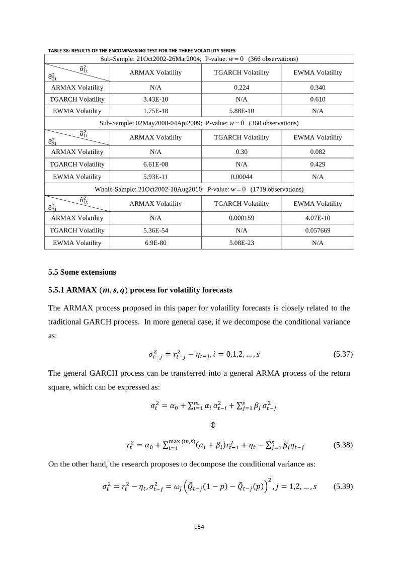
154

TABLE 38: RESULTS OF THE ENCOMPASSING TEST FOR THE THREE VOLATILITY SERIES

Sub-Sample: 21Oct2002-26Mar2004; P-value: 0w (366 observations)

ARMAX Volatility TGARCH Volatility EWMA Volatility

ARMAX Volatility N/A 0.224 0.340

TGARCH Volatility 3.43E-10 N/A 0.610

EWMA Volatility 1.75E-18 5.88E-10 N/A

Sub-Sample: 02May2008-04Api2009; P-value: 0w (360 observations)

ARMAX Volatility TGARCH Volatility EWMA Volatility

ARMAX Volatility N/A 0.30 0.082

TGARCH Volatility 6.61E-08 N/A 0.429

EWMA Volatility 5.93E-11 0.00044 N/A

Whole-Sample: 21Oct2002-10Aug2010; P-value: 0w (1719 observations)

ARMAX Volatility TGARCH Volatility EWMA Volatility

ARMAX Volatility N/A 0.000159 4.07E-10

TGARCH Volatility 5.36E-54 N/A 0.057669

EWMA Volatility 6.9E-80 5.08E-23 N/A

5.5 Some extensions

5.5.1 ARMAX process for volatility forecasts

The ARMAX process proposed in this paper for volatility forecasts is closely related to the

traditional GARCH process. In more general case, if we decompose the conditional variance

as:

(5.37)

The general GARCH process can be transferred into a general ARMA process of the return

square, which can be expressed as:

(5.38)

On the other hand, the research proposes to decompose the conditional variance as:

(5.39)

155

where is the symmetric quantile interval estimated from the returns

up to time

Substituting (5.39) into (5.38), we can obtain a general ARMAX process, which is

expressed as:

(5.40)

Compare ARMAX process (5.40) with ARMA process (5.38) , it can be seen that the major

difference is that instead of treating the lagged conditional variance terms as endogenous

variables that modeled by ARMA process of the return square, ARMAX model replace them

by the exogenous variable symmetric quantile intervals, which is estimated from the pre-

specified quantile regression model.

The ARMAX process is actually a special case of the regression (5.40) where and

are set both equal to one, that is:

(5.41)

A more general ARMAX for volatility forecast could be set if we do the following

substitution:

(5.42)

The ARMAX is obtained by substituting (5.42) into (5.38), which is expressed as:

(5.43)

The regression (5.43) could be served as the most general form for the volatility forecasts

proposed in this research. However, as the regression form becomes more complex, some

156

additional constraints of the parameters need to be set to ensure the unconditional variance

prediction to be positive. In this case, the ML estimation process will become more difficult

as well.

Besides, the research has not rigorously studied how to choose the optimal orders of the

ARMAX process for the volatility forecast. Since the low order of GARCH models are

commonly used in practice, we prefer the low order of ARMAX process for the volatility

forecasts as well.

In fact, we could easily transfer the low order of GARCH process into the low order of

ARMAX process, given that the ARMAX model has fairly close relationship with GARCH

model. For instance, the popular used type of GARCH , GARCH , GARCH ,

GARCH could be transferred into corresponding ARMAX , ARMAX ,

ARMAX and ARMAX .

Table 39 and 40 lists the estimation results of the ARMAX , ARMAX ,

ARMAX and ARMAX models for the randomly selected two sub-sample

periods and the whole sample period, based on the dataset we used in the section 5.4. It

could be seen that for each selected ARMAX model and each selected time-period, the

parameter which represents the effect of the symmetric quantile interval, is fairly

significant at 5% significant level. This confirms the robustness of the symmetric quantile

interval in the volatility forecast. Similarly, the coefficients of the first lag of the

autoregressive term shows high level of significance regardless of the specification of the

ARMAX model and the selection of the time periods, confirming the existence of the

clustering effect in time-varying volatility. It could also be found that the significance of the

first lag of the autoregressive term reduced when adding the second lag of the

autoregressive term into the ARMAX model. This is in fact a no surprising result, since

the two autoregressive terms will share some explanatory power with each other. The

coefficients of the constant, on the other hand, are always fairly small and insignificant,

indicating the drift term doesn’t exist in the time-varying daily volatility.

157

TABLE 39: PARAMETER ESTIMATION OF GENERAL ARMAX PROCESS ( TWO SUB-SAMPLE PERIODS)

Maximum Log Likelihood Value:

2007.074

Sub-Sample: 21Oct2002-01Jul2003

Number of Observations:252

ARMAX(1,0,1)

ttttt pQpQrr

2

112

1102 )(ˆ)1(ˆ

ARMAX(1,1,1)

tttttt pQpQrr 1

2

112

1102 )(ˆ)1(ˆ

Parameters Coef. P-value Parameters Coef. P-value

0 4.29e-06 0.969 .00007 0.284

1 0.304141 0.000 .5005646 0.000

0.065624 0.004 .0686498 0.000

1 .1134928 0.051

ARMAX(2,0,1)

tttttt pQpQrrr

2

222

222

1102 )(ˆ)1(ˆ

ARMAX(2,1,1)

ttttttt pQpQrrr 1

2

222

212

1102 )(ˆ)1(ˆ

Parameters Coef. P-value Parameters Coef. P-value

0 .0000697 0.277 0 .000081 0.468

1 .3943046 0.000 1 .30067 0.000

2 .0306967 0.431 2 .03220 0.000

.0688694 0.000 .0601913 0.000

.9312237 0.000

Maximum Log Likelihood Value:

1834.022

Sub-Sample: 01feb2006 - 28nov2006

Number of Observations:301

ARMAX(1,0,1)

ttttt pQpQrr

2

112

1102 )(ˆ)1(ˆ

ARMAX(1,1,1)

tttttt pQpQrr 1

2

112

1102 )(ˆ)1(ˆ

Parameters Coef. P-value Parameters Coef. P-value

.0000417 0.139 .0000159 0.344

.2548255 0.000 .220809 0.066

.057021 0.000 .0578665 0.000

1 .2962359 0.022

ARMAX(2,0,1)

tttttt pQpQrrr

2

222

222

1102 )(ˆ)1(ˆ

ARMAX(2,1,1)

ttttttt pQpQrrr 1

2

222

212

1102 )(ˆ)1(ˆ

Parameters Coef. P-value Parameters Coef. P-value

.0001364 0.061 0 .0002143 0.219

.031841 0.064 1 .0592891 0.070

2 .0248855 0.226 2 .0682887 0.367

.0564553 0.000 .0305709 0.079

.8431991 0.000

0

1

0 0

1 1

0

1

158

TABLE 40: PARAMETER ESTIMATION OF GENERAL ARMAX PROCESS (WHOLE-SAMPLE PERIOD)

Maximum Log Likelihood Value:

10962.49

Whole-Sample: 21Oct2002-10Aug2010

Number of Observations:1970

ARMAX(1,0,1)

ttttt pQpQrr

2

112

1102 )(ˆ)1(ˆ

ARMAX(1,1,1)

tttttt pQpQrr 1

2

112

1102 )(ˆ)1(ˆ

Parameters Coef. P-value Parameters Coef. P-value

0 .0000464 0.134 .0001634 0.196

1 .0919385 0.000 .9753181 0.000

.0727088 0.000 .062113 0.037

1 .8685472 0.000

ARMAX(2,0,1)

tttttt pQpQrrr

2

222

222

1102 )(ˆ)1(ˆ

ARMAX(2,1,1)

ttttttt pQpQrrr 1

2

222

212

1102 )(ˆ)1(ˆ

Parameters Coef. P-value Parameters Coef. P-value

0 .0000681 0.061 0 .0002318 0.205

1 .0957865 0.000 1 .8700192 0.000

2 .1301452 0.000 2 .1075984 0.000

.0598638 0.000 .0334481 0.000

.9312237 0.000

5.5.2 A comparison between ARMAX process and Taylor’s approach

Applying symmetric quantile interval into volatility forecast has been proposed by Taylor

(2005). In his research, a least squared regression is used for volatility prediction, which is

expressed as:

(5.44)

Since Taylor use the realized return square as the proxy for the actual variance

above regression could be rewritten as:

(5.45)

Compare this regression form with the ARMAX process proposed in this paper, which is:

(5.46)

The difference between these two regressions is essentially due to the different way of

processing the new information on time . For instance, given the same information set ,

Taylor’s approach utilize the whole information set to estimate ,

while the ARMAX process we proposed separate into and the new information

arrived on time (denote as ), in which is used to estimate

and is represent by

0

1

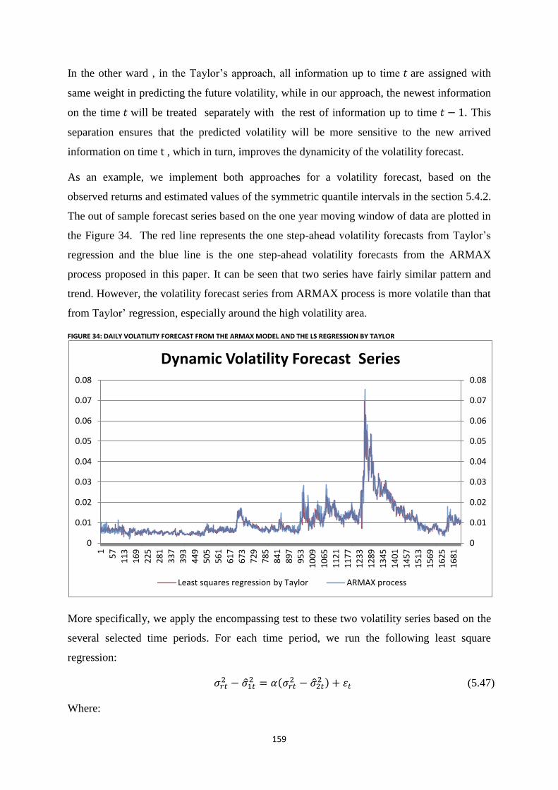
159

In the other ward , in the Taylor’s approach, all information up to time are assigned with

same weight in predicting the future volatility, while in our approach, the newest information

on the time will be treated separately with the rest of information up to time . This

separation ensures that the predicted volatility will be more sensitive to the new arrived

information on time , which in turn, improves the dynamicity of the volatility forecast.

As an example, we implement both approaches for a volatility forecast, based on the

observed returns and estimated values of the symmetric quantile intervals in the section 5.4.2.

The out of sample forecast series based on the one year moving window of data are plotted in

the Figure 34. The red line represents the one step-ahead volatility forecasts from Taylor’s

regression and the blue line is the one step-ahead volatility forecasts from the ARMAX

process proposed in this paper. It can be seen that two series have fairly similar pattern and

trend. However, the volatility forecast series from ARMAX process is more volatile than that

from Taylor’ regression, especially around the high volatility area.

FIGURE 34: DAILY VOLATILITY FORECAST FROM THE ARMAX MODEL AND THE LS REGRESSION BY TAYLOR

More specifically, we apply the encompassing test to these two volatility series based on the

several selected time periods. For each time period, we run the following least square

regression:

(5.47)

Where:

0

0.01

0.02

0.03

0.04

0.05

0.06

0.07

0.08

0

0.01

0.02

0.03

0.04

0.05

0.06

0.07

0.08

1

57

11

3

16

9

22

5

28

1

33

7

39

3

44

9

50

5

56

1

61

7

67

3

72

9

78

5

84

1

89

7

95

3

10

09

10

65

11

21

11

77

12

33

12

89

13

45

14

01

14

57

15

13

15

69

16

25

16

81

Dynamic Volatility Forecast Series

Least squares regression by Taylor ARMAX process

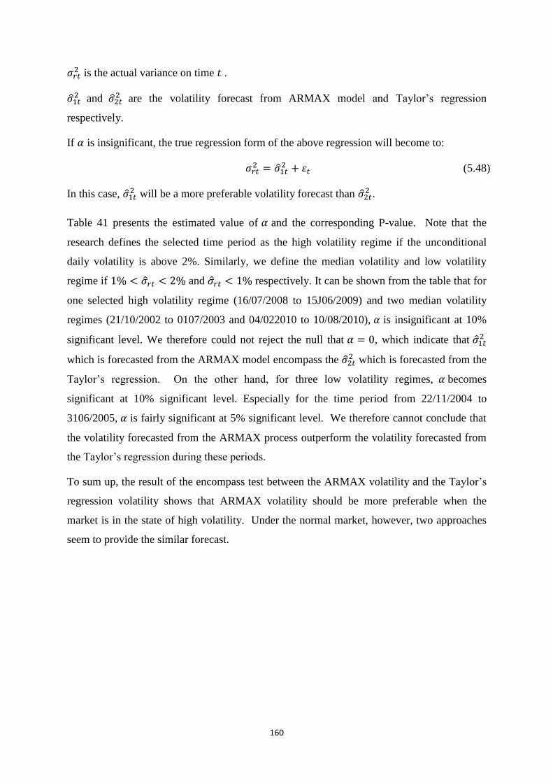
160

is the actual variance on time .

and

are the volatility forecast from ARMAX model and Taylor’s regression

respectively.

If is insignificant, the true regression form of the above regression will become to:

(5.48)

In this case, will be a more preferable volatility forecast than

.

Table 41 presents the estimated value of and the corresponding P-value. Note that the

research defines the selected time period as the high volatility regime if the unconditional

daily volatility is above 2%. Similarly, we define the median volatility and low volatility

regime if and respectively. It can be shown from the table that for

one selected high volatility regime (16/07/2008 to 15J06/2009) and two median volatility

regimes (21/10/2002 to 0107/2003 and 04/022010 to 10/08/2010), is insignificant at 10%

significant level. We therefore could not reject the null that , which indicate that

which is forecasted from the ARMAX model encompass the which is forecasted from the

Taylor’s regression. On the other hand, for three low volatility regimes, becomes

significant at 10% significant level. Especially for the time period from 22/11/2004 to

3106/2005, is fairly significant at 5% significant level. We therefore cannot conclude that

the volatility forecasted from the ARMAX process outperform the volatility forecasted from

the Taylor’s regression during these periods.

To sum up, the result of the encompass test between the ARMAX volatility and the Taylor’s

regression volatility shows that ARMAX volatility should be more preferable when the

market is in the state of high volatility. Under the normal market, however, two approaches

seem to provide the similar forecast.

161

TABLE 41: ENCOMPASSING TEST BETWEEN THE ARMAX VOLATILITY AND THE VOLATILITY FROM TAYLOR’S REGRESSION

Time periods Parameter

Std

(P-value) ttttRt )ˆˆ(ˆ 2

221

21

2 Unconditional

Volatility

21Oct2002 to

01Jul2003 .3117914 .359(0.387)

Median volatility Time

Period 0.83%

16Jul2008 to

15Jun2009 .0599474 .191(0.754) High volatility Time Period 2.8%

04Feb2010 to

10Aug2010 .5613849 .354(0.115)

Median volatility Time

Period 1.3%

24Dec2003-

10May2004 .4279934 .256(0.096) Low volatility Time Period 0.43%

22Nov2004-31Jun2005 .5501106 .255(0.032) Low volatility Time Period 0.35%

16Aug2005-

01May2006 .5146068 .284(0.072)

Median volatility Time

Period 1.32%

5.6 Conclusion

Volatility modeling plays a important role in the market risk measurement. Motivated by the

Taylor’s research of forecasting volatility from VaR estimate, we proposed a new type of

ARMAX process for volatility forecast in this chapter. More explicitly, instead of using the

Taylor’s regression for volatility forecast, we adopt the idea from GARCH process, in which

the conditional variance is modeled by a general ARMA process of the return square. The

innovation of the model lies in that it replace the lagged conditional variance terms in

GARCH model by the exogenous variable, which is the symmetric quantile intervals

estimated from the pre-specified quantile regression model. This amendment relaxes the

assumption about the value of the unobserved true variance in the parameter estimation

procedure and could therefore generate a more reasonable volatility forecast.

The major difference between this model and Taylor’s regression is essentially based on the

different way of processing the new information on time . Compared to the Taylor’s

regression model which use all the information up to time to estimate the symmetric

Quantile, this model separate the newest information on the time and the rest of the

information up to time . This separation ensures that the predicted volatility will be

more sensitive to the new arrived information on time , which improves the dynamicity of

the model forecast. Besides, we proposed a new specified quantile regression model for the

symmetric quantile interval estimation, which has a separate function forms for the left and

the right Quantile. This specification is aim to improve the accuracy of the symmetric

162

quantile estimates, which in turn, improve the accuracy of the corresponding volatility

forecast.

163

6. Final Remarks

Risk modeling is a core part of any risk management system. In financial markets, although

extreme price movements are rare, they can have serious consequences resulting in huge

economic losses and can even threaten the survival of firms. Accurate and valid risk

modeling allows risk managers to detect and understand such risk properly, so they can

consciously plan and control the potential adverse outcomes resulting from such risk.

An essential part of the financial risk modeling tool kit is the Value at Risk (VaR)

methodology. VaR’s dominance stems from the regulatory and economic incentives and also

from its computational appeal. Deregulation in the early of 1990s led to a growing number of

commercial banks offering investment banking services, which significantly increased their

financial risk exposure. As a result many banks developed proprietary internal risk models.

JP Morgan, on the other hand, advanced a risk measurement methodology (named

) available to the public, in which the central element is the VaR methodology.

Applying probability theory, VaR summarize the overall financial risk in a single potential

dollar loss. Compared to other traditional risk measures, VaR possesses both computational-

appealing and forward-looking properties, which allows users to quantify the financial risk in

an accurate, inexpensive and timely manner.

Since its initial appearance in middle of the 1990s, the VaR technique has undergone a

considerable revolution and development during the last 15 years. The use of VaR has also

spread from simple quantification of financial risk to an active control and management tool.

In the market amendments of the Basel accord in 1998 and Basel II accord in 2004, the

Bank for International Settlements (BIS) endorsed internally developed capital requirements

for commercial banks directly related to VaR, further solidifying the popularity of this risk

measurement technique.

My PhD research focuses on the VaR methodology. Although this risk measurement tool is

conceptually simple and has been well-accepted as the benchmark of the market risk

quantification, risk managers do encounter some difficulties in the practical application of

this measure. An issue of most concern is how to select the optimal VaR model under the

different market condition and different risk factors. Furthermore, given that the conditional

distribution of the market risk factors changes over time, how to improve the dynamicity of

the VaR models is also an important consideration for the further development of the modern

risk management industry.

164

The existence of these issues provides the motivation for this research. Reviewing the

structure of the thesis: after a comprehensive and systematic study of existing VaR

techniques in chapter one, chapter two undertakes a complete empirical analysis of the model

application based on the historical and simulated data, from which we formulate some

applicable selection criteria for different market conditions and different asset categories.

These empirical findings also provide useful information on model improvement and

contribute to the model innovations which I then propose. More explicitly, I propose two

newly developed risk models. Chapter four proposes a Two-Step Dynamic Adjusted CAViaR

model for dynamic VaR generation and chapter five proposes an ARMAX model for

dynamic volatility forecasting. Both models are derived by integrating volatility modeling

and the quantile regression technique, which enhance the models predictive ability. These

two models serve as the key research outcomes from my PhD research.

This research has some limitations which need to be mentioned: Firstly, the content of the

research is purely quantitative. The intensively using the numerical data in the risk modeling

will inevitably leads to data measurement error and bias. For instance, the historical data used

this research are purely collected from Thomason Reuters DataStream. Instead of actual price

series, these collected data may be the appraisal data which has already been smoothed by the

data provider. The use of the appraisal data might results in correlations and standard

deviation that are biased downwards31

, which misrepresent the true volatility in the market.

Furthermore, given that the output risk estimates form the VaR models are solely dependents

on the input data, the choice of the time span of the input data will be critically important in

the risk modeling. There is a tradeoff between using a time span of data that is too short or

too long. On one hand, a long time span of data is required by the statistical measures for the

stability and precision of the parameter estimates. On the other hand, longer time spans of

data will increase the probability of regime changes and non-stationary data, which reduce

the reliability of the model forecast. In this research, we normally select the moving data

window as 1 year for model estimation if daily frequency is considered. This setting, however,

might not be the optimal choice in practice. A competent risk manager should be able to use

his experience and knowledge to judge which time span of data is the optimal input data to

generate the risk expectation. For this perspective, a good risk manger is not only a good

econometrician but also a good economist.

31

Source from: Capital Market Expectation, Level III 2012 (CFA Program Curriculum Volume 2)

165

Finally, the risk modeling techniques covered in this research are derived under traditional

financial assumptions, where investors are assumed to be rational and make investment

decision restrictively according to the modern portfolio theory. Under this framework,

investors exhibit risk aversion and seek to maximize the return at the given level of risk. In

reality, however, market participant might employ some combination of traditional finance

and psychological biases when making their investment decisions. For instance, instead of

seeking risk minimization and return maximization, a market participant will exhibit loss

aversion and make utility-maximizing decisions based on all available information.

Despite these limitations, quantitative risk modeling is indispensible to the modern risk

management system. Unlike other processes in the system, which tend to be descriptive in

nature, risk modeling is prescriptive and can provide clear statements about the level of risk

now and in the future. The model improvements and extensions proposed in this PhD aim to

support risk mangers and help improve risk modeling.

166

References

Artigas, J., Tsay, R., 2003. Effective estimation of stochastic diffusion models with leverage

effects and jumps. Working paper. Graduate School of Business, University of Chicago.

Artzner, P., Delbaen, F., 1999. Coherent measures of risk. Mathematical Finance, 203-28.

Balkema, A., Laurens, D., 1974. Residual life time at great age. Annals of Probability 2, 792-

804.

Bao, Y., Lee, T., Saltoglu, B., 2006. Evaluating predictive performance of value at risk

models in emerging markets: a reality check. Journal of Forecasting 25, 101-28.

Beirlant, J., Teugels, J., Vynckier, P., 1996. Practical analysis of extreme values. Leuven

University Press, Leuven.

Bollerslev, T., 1986. Generalized autoregressive conditional heteroscedasticity. Journal of

Econometrics 31, 307-327.

Bollerslev, T., Chou, R., 1992. ARCH modeling in finance. Journal of Econometrics 52, 5-

59.

Boudoukh, J., Richardson, M., Whitelaw, R., 1998. The best of both worlds. Risk 11, 64-67.

Cai, Z., Wang, X., 2008. Nonparametric estimation of conditional VaR and expected

shortfall. Journal of Econometric 147, 120-130.

Carlin, P., Stoffer, 1992. A Monte Carlo approach to nonnormal and nonlinear state space

modeling. Journal of the American Statistical Association 87, 493-500.

Chernozhukov, V., Umantsev, L., 2000. Conditional value at risk: Aspects of modeling and

estimation. Unpublished working paper. Massachusetts Institute of Technology.

Christoffersen, P., 1998. Evaluating interval forecasts. International Economic Review 39,

841-862.

167

Danielsson, J., Vries, C., 2000. Value-at-risk and extreme returns. Annales d'economie et de

statistique 60, 236-269.

Danielsson, J., 2011. Financial risk forecasting: the theory and practice of forecasting market

risk with implementation in R and Matlab. Wiley-Blackwell Press, UK.

Delbaen, F., 2002. Coherent risk measures on general probability spaces, advances in finance

and stochastics. Essays in Honour of Dieter Sondermann, Springer-Verlag, 1–37.

Dowd, K., 1998. Beyond value at risk: The new science of risk management. Wiley-

Blackwell Press, UK.

Duffie, D., Pan, J., 1997. An overview of value at risk. The Journal of Derivatives 6, 7-49.

Duffie, D., Rohit, R., 1995. Financial market innovation and security design: An introduction.

Journal of Economic Theory 65, 1-42.

Edwin, J., Martin, J., 2009. Modern portfolio theory and investment analysis. John Wiley&

Sons Press, UK.

Engle, R., Manganelli, S., 2004. CAViaR: Conditional autoregressive value at risk by

regression quantile. Journal of Business Economic Statisticsl 22, 367-381.

Erev, I., Ert, E., Yechiam, E., 2008. Loss aversion, diminishing sensitivity, and the effect of

experience on repeated decisions. Journal of Behavioral Decision Making 21, 575-597.

Everitt, B., 2002. The cambridge dictionary of statistics. Cambridge University Press, UK.

Gaglianone, W., 2009. Evaluating value-at-risk models via quintile regression. Working

Paper. Departamento de Economía, Universidad Carlos III de Madrid.

Giot, P., Laurent, S., 2004. Modeling daily value-at-risk using realized volatility and ARCH

type models. Journal of Empirical Finance 11, 379-398.

168

Glosten, L., Jagannathan, R., Runkle, D., 1993. On the relation between the expected value

and the volatility of the nominal excess return on stocks. Journal of Finance 48, 1779-1801.

Granger, C., Newbold, P., 1986. Forecasting economic time series. 2nd ed. Academic Press,

Orlando.

Guoliang, L., Luqin, L., 2007. Convergence rate of the estimate of the regression function

under martingale difference sequence. J. Sys. Sci. & Math. Scis 27, 152-160.

Harvey, A., Ruiz, E., Shephard, N., 1994. Multivariate stochastic variance models. Journal of

Business & Economic Statistics 12, 371-417.

Henrard, M., 2000. Comparison of cash flow maps for value-at-risk. Journal of Risk 3, 57-71.

Hsieh, D., 1993. Implications of nonlinear dynamics for financial risk management. Journal

of Financial and Quantitative Analysis 28, 41-64.

Huang, A., Yihou, 2009. A value at risk approach with kernel estimator. Applied Financial

Economics 19, 379-395.

Hull, J., 2008. Options, futures and other derivatives. 7th ed. Pearson Press, UK.

Jacquier, E., Polson, N., Rossi, P., 1994. Bayesian analysis of stochastic volatility models:

reply. Journal of Business & Economic Statistics 12, 413-417.

Jeon, J., Taylor, J., 2010. Using implied volatility with CAViaR models for value at risk

estimation. Journal of Forecasting, forthcoming.

Jorion, P., 2006. Value at risk: The new benchmark for managing financial risk. 3rd ed.

McGraw-Hill Press, New York.

Jose, A., Lopez, C., Walter, 2001. Evaluating covariance matrix forecasts in a value-at-risk

framework. Journal of Risk 3.

169

Kim, T., White, H., 2002. Estimation, inference, and specification testing for possibly

misspecified quantile regressions. Advances in Econometrics 17, 107-132.

Koenker, R., 2005. Quantile regression. Cambridge University Press, UK.

Koenker, R., Bassett, G., 1978. Regression quantile. Econometrica 46, 33-50.

Koenker, R., d'Orey, V., 1993. Computing dual regression quantiles and regression rank

scores. Statist 43, 410-414.

Koenker, R., Zhao, Q., 1996. Conditional quantile estimation and inference for ARCH

models. Econometric Theory 12, 793-813.

Kuersteiner, G., 2000. RMSE reduction for GMM estimators of linear time series models.

Econometric Society World Congress 2000 Contributed Papers. Econometric Society.

Kupiec, P., 1995. Techniques for verifying the accuracy of risk measurement models. Journal

of Derivatives 3, 73-84.

Li, M., Lin, H., 2004. Estimating value-at-risk via Markov switching ARCH models – an

empirical study on stock index returns. Applied Financial Economics 11, 679-91.

Marc, P., Henrard, 2000. Comparison of cash flow maps for value-at-risk. The Journal of

Risk 3, 57-71.

Mayhew, S., 1995. Implied volatility. Financial Analysts Journal 51, 8-20.

McNeil, A., 1999. Extreme value theory for risk managers. Risk Books, 93-113.

McNeil, A., Frey, R., Embrechts, P., 2005. Quantitative risk management: Concepts,

techniques and tools. Princeton University Press.

170

McNeil, A., Frey, R., 2000. Estimation of tail-related risk measures for heteroscedastic

financial time series: an extreme value approach. Journal of Empirical Finance 7, 271-300.

Merton, R., 1976. Option pricing when underlying stock returns are discontinuous. Journal of

Financial Economics 3, 125-144.

Mittnik, S., Paolella, M., Rachev, S., 2002. Stationary of stable power-GARCH processes.

Journal of Econometrics 106, 97-107.

Mukherjee, K., 1999. Asymptotics of quantile and rank scores in nonlinear time series.

Journal of Time Series Analysis 20, 173-192.

Nelson, D., 1991. Conditional heteroskedasticity in asset returns: A new approach.

Econometrica 59, 347-370.

Oksendal, Bernt, K., 2002. Stochastic differential equations: An introduction with

applications. Springer, 326.

Pearson, K., 1901. On lines and planes of closest fit to systems of points in space.

Philosophical Magazine 2, 559-572.

Pearson, S., Tukey, J., 1965. Approximate means and standard deviations based on distances

between percentage points of frequency curves. Biometrika 52, 533-546.

Peter, Z., 1996. Riskmetrics technical document. Riskmetrics Monitor. Reuters/JP Morgan.

Pickands, J., 1975. Statistical inference using extreme order statistics. Annals of Statistics 3,

119-131.

Poon, S., Granger, C., 2003. Forecasting volatility in financial markets: A review. Journal of

Economic Literature 41, 478-639.

171

Portnoy, S., 1991. Asymptotic behavior of regression quantile in nonstationary, dependent

cases. Journal of Multivariate Analysis 38, 100–113.

Rydberg, T., Shephard, N., 2003. Dynamics of trade by trade price movements:

Decomposition and models. Journal of Financial Econometrics 1, 2-25.

Schaumburg, S., 2010. Predicting extreme VaR: Nonparametric quantile regression with

refinements from extreme value theory. SFB 649 Discussion Papers. Humboldt University,

Berlin, Germany.

Sharpe, W., 1966. Mutual fund performance. Journal of Business 39, 119-138.

Sharpe, W., 1964. Capital asset prices: A theory of market equilibrium under conditions of

risk. Journal of Finance 19, 425-42.

Shaw, P., 2003. Multivariate statistics for the environmental sciences. Hodder-Arnold Press,

New York.

Shephard , N., 2003. Stochastic volatility. Oxford University Press, UK.

Stuart, A., Ord, J., 1994. Kendall's advanced theory of statistics. Edward-Arnold Press, New

York.

Taylor, J., 2005. Generating volatility forecasts from value at risk estimates. Management

Science 51, 712-725.

Taylor, S., 1994. Modelling stochastic volatility: a review and comparative study.

Mathematical Finance 4, 183-204.

Tsay, R., 1986. Nonlinearity tests for time series. Biometrika 73, 461-466.

Tsay, R., 2005. Analysis of financial time series. 2rd ed. Academic Press, New York.

172

Value-at-risk: An overview of analytical VaR. J.P. Morgan Investment Analytics Consulting

Quarterly Newsletter, September 2008.

Venkataraman, S., 1997. Value at risk for a mixture of normal distributions: the use of quasi-

Bayesian estimation techniques. Economic Perspectives, 2-13.

Weiss, A., 1991. Estimating nonlinear dynamic models using least absolute error estimation.

Econometric Theory 7, 46-68.

Wilson, T., 1994. Plugging the GAP. Risk 7, 74-80.

Yu, K., Jones, M., 1998. Local Linear Quantile Regression. Journal of the American

Statistical Association 93, 228-237.