Embed Size (px)
Citation preview

Topics in Combinatorial DifferentialTopology and Geometry
Robin Forman


IAS/Park City Mathematics SeriesVolume 14, 2004
Topics in Combinatorial DifferentialTopology and Geometry
Robin Forman
Many questions from a variety of areas of mathematics lead one to the problemof analyzing the topology or the combinatorial geometry of a simplicial complex.We will see a number of examples in these notes. Some very general theories havebeen developed for the investigation of similar questions for smooth manifolds. Ourgoal in these lectures is to show that there is much to be gained in the world ofcombinatorics from borrowing questions, tools, motivation, and even inspirationfrom the theory of smooth manifolds.
These lectures center on two main topics which illustrate the dramatic impactthat ideas from the study of smooth manifolds have had on the study of combina-torial spaces. The first topic has its origins in differential topology, and the secondin differential geometry.
One of the most powerful and useful tools in the study of the topology of smoothmanifolds is Morse theory. In the first three lectures we present a combinatorialMorse theory that posesses many of the desirable properties of the smooth theory,and which can be usefully applied to the study of very general combinatorial spaces.In the first two lectures we present the basic theory along with numerous examples.In the third lecture, we show that discrete Morse theory is a very natural tool forthe study of some questions in complexity theory.
Much of the study of global differential geometry is concerned with the rela-tionship between the geometry of a Riemannian manifold and its topology. Onelong conjectured, still unproved, relationship is the Hopf conjecture, which statesthat if a manifold has nonpositive sectional curvature, then the sign of its Eulercharacteristic depends only on its dimension. (See Lecture 4 for a more precisestatement.) In [15] Charney and Davis formulated a combinatorial analogue of
1The Department of Mathematics, Rice University, Houston, TX, USA 77251.E-mail address: [email protected] author was supported in part by the National Science Foundation. The author would alsolike to thank Carsten Lange, who served as the TA for these lectures, created most of the figuresin these notes, and whose enthusiasm and attention to detail dramatically increased the com-prehensibility of the text. The author expresses his gratitude to the organizers of the IAS/PCSummer Institute for their tireless dedication and enthusiasm for all things organizational andmathematical. Their support greatly improved the lectures and these notes.
c©2007 American Mathematical Society
135
136 R. FORMAN, COMB. DIFFERENTIAL TOPOLOGY AND GEOMETRY
this conjecture, and then observed that their conjecture is related to some of thecentral questions in geometric combinatorics. There has been some fascinating re-cent work on this subject, which has resulted in some very tantalizing, more generalconjectures. In Lectures 4 and 5 we present an introduction to the conjectures ofCharney and Davis, discuss some of the known partial results, and survey the mostrecent developments.
LECTURE 1Discrete Morse Theory
1. Introduction
There is a very close relationship between the topology of a smooth manifold Mand the critical points of a smooth function f on M . For example, if M is compact,then f must achieve a maximum and a minimum. Morse theory is a far-reachingextension of this fact. Milnor’s beautiful book [71] is the standard reference onthis subject. In these notes we present an adaptation of Morse theory that may beapplied to any simplicial complex (or more general cell complex). There have beenother adaptations of Morse Theory that can be applied to combinatorial spaces. Forexample, a Morse Theory of piecewise linear functions appears in [59] and the verypowerful “Stratified Morse Theory” was developed by Goresky and MacPherson[46],[47]. These theories, especially the latter, have each been successfully appliedto prove some very striking results.
We take a slightly different approach than that taken in these references. Ratherthan choosing a suitable class of continuous functions on our spaces to play the roleof Morse functions, we will be working entirely with discrete structures. Hence, wehave chosen the name discrete Morse theory for the ideas we will describe. More-over, in these notes, we will describe the theory entirely in terms of the (discrete)gradient vector field, rather than an underlying function. We show that even with-out introducing any continuity, one can recreate, in the category of combinatorialspaces, a complete theory that captures many of the intricacies of the smooth the-ory, and can be used as an effective tool for a wide variety of combinatorial andtopological problems.
The goal of these lectures is to present an overview of the subject of discreteMorse theory that is sufficient both to understand the major applications of thetheory to combinatorics, and to apply the the theory to new problems. We willnot be presenting theorems in their most recent or most general form, and simpleexamples will often take the place of proofs. Those interested in a more completepresentation of the theory can consult the reference [32]. Earlier surveys of thiswork have appeared in [31] and [35], and earlier, and similar, versions of some ofthe sections in these notes appeared in [39] and [40].
137

138 R. FORMAN, COMB. DIFFERENTIAL TOPOLOGY AND GEOMETRY
2. Cell Complexes and CW Complexes
The main theorems of discrete (and smooth) Morse theory are best stated in thelanguage of CW complexes, so we begin with an overview of the basics of suchcomplexes. J. H. C. Whitehead introduced CW complexes in his foundational workon homotopy theory, and all of the results in this section are due to him. Thereader should consult [68] for a very complete introduction to this topic. In thesenotes we will consider only finite CW complexes, so many of the subtleties of thesubject will not appear.
The building blocks of cell complexes are cells. Let Bd denote the closed unitball in d-dimensional Euclidean space. That is, Bd = {x ∈ Ed s.t. |x| ≤ 1}. Theboundary of Bd is the unit (d − 1)-sphere S(d−1) = {x ∈ Ed s.t. |x| = 1}. A d-cellis a topological space which is homeomorphic to Bd. If σ is d-cell, then we denoteby σ the subset of σ corresponding to S(d−1) ⊂ Bd under any homeomorphismbetween Bd and σ. A cell is a topological space which is a d-cell for some d.
The basic operation of cell complexes is the notion of attaching a cell. Let Xbe a topological space, σ a d-cell and f : σ → X a continuous map. We let X ∪f σdenote the disjoint union of X and σ quotiented out by the equivalence relationthat each point s ∈ σ is identified with f(s) ∈ X . We refer to this operation bysaying that X ∪f σ is the result of attaching the cell σ to X . The map f is calledthe attaching map.
We emphasize that the attaching map must be defined on all of σ. That is,the entire boundary of σ must be “glued” to X . For example, if X is a circle, thenFigure 1(i) shows one possible result of attaching a 1-cell to X . Attaching a 1-cellto X cannot lead to the space illustrated in Figure 1(ii) since the entire boundaryof the 1-cell has not been “glued” to X .
We are now ready for our main definition. A finite cell complex is any topo-logical space X such that there exists a finite nested sequence
(1) ∅ ⊂ X0 ⊂ X1 ⊂ · · · ⊂ Xn = X
such that for each i = 0, 1, 2, . . . , n, Xi is the result of attaching a cell to X(i−1).Note that this definition requires that X0 be a 0-cell. If X is a cell complex, we
refer to any sequence of spaces as in (1) as a cell decomposition of X . Suppose that
(i) (ii)Figure 1. On the left a 1-cell is attached to a circle. This is not true for thepicture on the right.

LECTURE 1. DISCRETE MORSE THEORY 139
X0 X1 X2 X3
Figure 2. A cell decomposition of the torus.
in the cell decomposition (1), of the n + 1 cells that are attached, exactly cd ared-cells. Then we say that the cell complex X has a cell decomposition consistingof cd d-cells for every d.
We note that a (closed) d-simplex is a d-cell. Thus a finite simplicial complexis a cell complex, and has a cell decomposition in which the cells are precisely theclosed simplices.
In Figure 2 we demonstrate a cell decomposition of a 2-dimensional torus which,beginning with the 0-cell, requires attaching two 1-cells and then one 2-cell. Here wecan see one of the most compelling reasons for expanding our view from simplicialcomplexes to more general cell complexes. Every simplicial decomposition of the2-torus has at least 7 vertices, 21 edges and 14 triangles.
It may seem that quite a bit has been lost in the transition from simplicialcomplexes to general cell complexes. After all, a simplicial complex is completelydescribed by a finite amount of combinatorial data. On the other hand, the con-struction of a cell decomposition requires the choice of a number of continuousmaps. However, if one is only concerned with the homotopy type of the resultingcell complex, then things begin to look a bit more manageable. Namely, the homo-topy type of X ∪f σ depends only on the homotopy type of X and the homotopyclass of f .
Theorem 1. Let h : X → X ′ denote a homotopy equivalence, σ a cell, and f1 :σ → X, f2 : σ → X ′ two continuous maps. If h ◦ f1 is homotopic to f2, thenX ∪f1 σ and X ′ ∪f2 σ are homotopy equivalent.
(See Theorem 2.3 on page 120 of [68].) An important special case is when h is theidentity map. We state this case separately for future reference.
Corollary 2. Let X be a topological space, σ a cell, and f1, f2 : σ → X twocontinuous maps. If f1 and f2 are homotopic, then X ∪f1 σ and X ∪f2 σ arehomotopy equivalent.
Therefore, the homotopy type of a cell complex is determined by the homotopyclasses of the attaching maps. Since homotopy clases are discrete objects, we havenow recaptured a bit of the combinatorial atmosphere that we seemingly lost whengeneralizing from simplicial complexes to cell complexes.
Let us now present some examples.1) Suppose X is a topological space which has a cell decomposition consisting
of exactly one 0-cell and one d-cell. Then X has a cell decomposition ∅ ⊂ X0 ⊂X1 = X . The space X0 must be the 0-cell, and X = X1 is the result of attachingthe d-cell to X0. Since X0 consists of a single point, the only possible attachingmap is the constant map. Thus X is constructed from taking a closed d-ball and

140 R. FORMAN, COMB. DIFFERENTIAL TOPOLOGY AND GEOMETRY
identifying all of the points on its boundary. One can easily see that this impliesthat the resulting space is a d-sphere.
2) Suppose X is a topological space which has a cell decomposition consisting ofexactly one 0-cell and n d-cells. Then X has a cell decomposition as in (1) such thatX0 is the 0-cell, and for each i = 1, 2, . . . , n the space Xi is the result of attachinga d-cell to X(i−1). From the previous example, we know that X1 is a d-sphere.The space X2 is constructed by attaching a d-cell to X1. The attaching map is acontinuous map from a (d− 1)-sphere to X1. Every map of the (d− 1)-sphere intoX1 is homotopic to a constant map (since π(d−1)(X1) ∼= π(d−1)(Sd) ∼= 0). If theattaching map is actually a constant map, then it is easy to see that the space X2
is the wedge of two d-spheres, denoted by Sd ∨ Sd. (The wedge of a collection oftopological spaces is the space resulting from choosing a point in each space, takingthe disjoint union of the spaces, and identifying all of the chosen points.) Since theattaching map must be homotopic to a constant map, Corollary 2 implies that X2
is homotopy equivalent to a wedge of two d-spheres.When constructing X3 by attaching a d-cell to X2, the relevant information is a
map from Sd−1 to X2, and the homotopy type of the resulting space is determinedby the homotopy class of this map. All such maps are homotopic to a constantmap (since πd−1(X2) ∼= πd−1(Sd ∨ Sd) ∼= 0). Since X2 is homotopy equivalent toa wedge of two d-spheres, and the attaching map is homotopic to a constant map,it follows from Theorem 1 that X3 is homotopy equivalent to the space that wouldresult from attaching a d-cell to Sd ∨ Sd via a constant map, i.e. X3 is homotopyequivalent to a wedge of three d-spheres.
Continuing in this fashion, we can see that X must be homotopy equivalent toa wedge of n d-spheres.
The reader should not get the impression that the homotopy type of a cell com-plex is determined by the number of cells of each dimension. This is true only forvery few spaces (and the reader might enjoy coming up with some other examples).The fact that wedges of spheres can, in fact, be identified by this numerical datapartly explains why the main theorem of many papers in combinatorial topologyis that a certain simplicial complex is homotopy equivalent to a wedge of spheres.Namely such complexes are the easiest to recognize. However, that does not ex-plain why so many simplicial complexes that arise in combinatorics are homotopyequivalent to a wedge of spheres. I have often wondered if perhaps there is somedeeper explanation for this.
3) Suppose that X is a cell complex which has a cell decomposition consistingof exactly one 0-cell, one 1-cell and one 2-cell. Let us consider a cell decompositionfor X with these cells: ∅ ⊂ X0 ⊂ X1 ⊂ X2 = X. We know that X0 is the 0-cell.Suppose that X1 is the result of attaching the 1-cell to X0. Then X1 must be acircle, and X2 arises from attaching a 2-cell to X1. The attaching map is a mapfrom the boundary of the 2-cell, i.e. a circle, to X1 which is also a circle. Up tohomotopy, such a map is determined by its winding number, which can be takento be a nonnegative integer. If the winding number is 0, then without altering thehomotopy type of X we may assume that the attaching map is a constant map,which yields that X ∼ S1 ∨ S2 (where ∼ denotes homotopy equivalence). If thewinding number is 1 then without altering the homotopy type of X we may assumethat the attaching map is a homeomorphism, in which case X is a 2-dimensionaldisc. If the winding number is 2, then without altering the homotopy type of X

LECTURE 1. DISCRETE MORSE THEORY 141
we may assume that the attaching map is a standard degree 2 mapping (i.e. thatwraps one circle around the other twice, with no backtracking). The reader shouldconvince him/herself that the result in this case is that X is the 2-dimensionalprojective space P2. In fact, each winding number results in a homotopically distinctspace. These spaces can be distinguished by their homology, since H1(X, Z) for thespace X resulting from an attaching map with winding number n is isomorphic toZ/nZ.
It seems that we are not quite done with this example, because we assumedthat the 1-cell was attached before the 2-cell, and we must consider the alternativeorder, in which X1 is the result of attaching a 2-cell to X0. In this case, X1 is a2-sphere, and X = X2 is the result of attaching a 1-cell to X1. The attaching mapis a map of S0 into S2. Since S2 is connected (i.e. π0(S2) = 0) all such maps arehomotopic to a constant map. Taking the attaching map to be a constant mapyields that X = S1 ∨ S2. Thus adding the cells in this order merely resulted infewer possibilities for the homotopy type of X . This is a general phenomenon.Generalizing the argument we just presented, using the fact that πi(Sd) = 0 fori < d, yields the following statement.
Proposition 3. Let
(2) ∅ ⊂ X0 ⊂ X1 ⊂ · · · ⊂ Xn = X
be a cell decomposition of a finite cell complex X. Then X is homotopy equivalent toa finite cell decomposition with precisely the same number of cells of each dimensionas in (2), and with the cells attached so that their dimensions form a nondecreasingsequence.
A CW complex is one that can be constructed in this fashion. In fact, evenmore is required.
Definition 4. A CW complex is a cell complex with the property that the boundaryof each cell is mapped into the union of the cells of lower dimension.
In some sense, this is a merely technical requirement, as every cell complexis homotopy equivalent to a CW complex. However, there are certain advantagesto working with CW complexes, and all of the cell complexes which arise in thesenotes will be CW complexes.
I first learned of simplicial complexes in a course on algebraic topology. Theywere introduced as a category of topological spaces for which it was rather easy todefine homology and cohomology, i.e. in terms of the simplical chain- and cochain-complexes. One might be concerned that in the transition from simplicial complexesto cell complexes we have lost this ability to easily compute these topological in-variants. In fact, much of this computability remains. Let X be a cell complexwith a fixed cell decomposition. Suppose that in this decomposition X is con-structed from exactly cd cells of dimension d for each d = 0, 1, 2, . . . , n = dim(K),and let Cd(X, Z) denote the space Zcd (more precisely, Cd(X, Z) denotes the freeabelian group generated by the d-cells of X , each endowed with an orientation).The following is one of the fundamental results in the theory of cell complexes.
Theorem 5. There are boundary maps ∂d : Cd(X, Z) → Cd−1(X, Z), for each d,so that
∂d−1 ◦ ∂d = 0
142 R. FORMAN, COMB. DIFFERENTIAL TOPOLOGY AND GEOMETRY
and such that the resulting differential complex
0 −−−−→ Cn(X, Z) ∂n−−−−→ . . .∂1−−−−→ C0(X, Z) −−−−→ 0
calculates the homology of X. That is, if we define
Hd(C, ∂) =Ker(∂d)Im(∂d+1)
,
then for each d
Hd(C, ∂) ∼= Hd(X, Z),
where Hd(X, Z) denotes the singular homology of X.
The actual definition of the boundary map ∂ is slightly nontrivial and we will notgo into it here (see [68, Ch. V, Sec. 2] for the details). In fact, it is here that wesee the main distinction between general cell complexes and CW complexes. Theremay exist multiple choices for the boundary map for a general cell complex, but theboundary map is canonical for a CW complex. At first it may seem that withoutknowing this boundary map, there is little to be gained from Theorem 5. In fact,much can be learned from just knowing of the existence of such a boundary map.For example, let us choose a coefficient field F, and tensor everything with F to geta differential complex
0 −−−−→ Cn(X, F) ∂n−−−−→ . . .∂1−−−−→ C0(X, F) −−−−→ 0
which calculates H∗(X, F), where now Cd(X, F) ∼= Fcd .
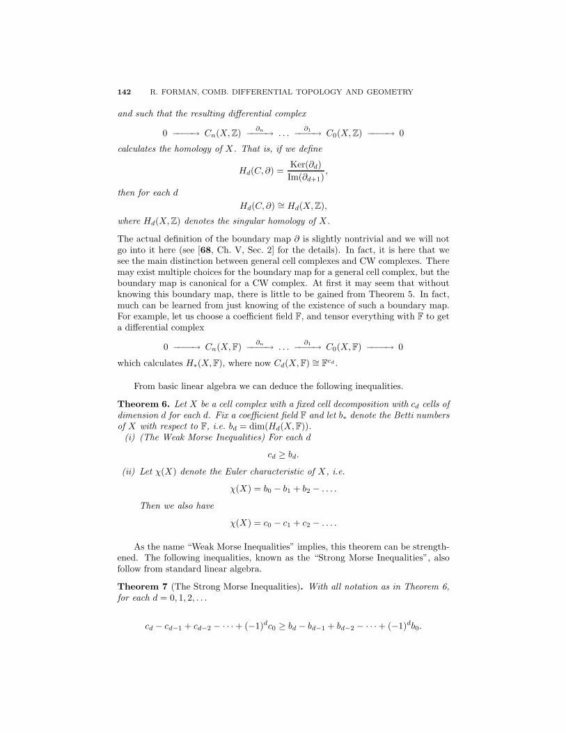
From basic linear algebra we can deduce the following inequalities.
Theorem 6. Let X be a cell complex with a fixed cell decomposition with cd cells ofdimension d for each d. Fix a coefficient field F and let b∗ denote the Betti numbersof X with respect to F, i.e. bd = dim(Hd(X, F)).
(i) (The Weak Morse Inequalities) For each d
cd ≥ bd.
(ii) Let χ(X) denote the Euler characteristic of X, i.e.
χ(X) = b0 − b1 + b2 − . . . .
Then we also have
χ(X) = c0 − c1 + c2 − . . . .
As the name “Weak Morse Inequalities” implies, this theorem can be strength-ened. The following inequalities, known as the “Strong Morse Inequalities”, alsofollow from standard linear algebra.
Theorem 7 (The Strong Morse Inequalities). With all notation as in Theorem 6,for each d = 0, 1, 2, . . .
cd − cd−1 + cd−2 − · · · + (−1)dc0 ≥ bd − bd−1 + bd−2 − · · · + (−1)db0.
LECTURE 1. DISCRETE MORSE THEORY 143
As the names imply, Theorem 7 does directly imply Theorem 6, as one can see bycomparing Strong Morse Inequalities for consecutive values of d, and using the factthat bi = 0 for i larger than the dimension of K.
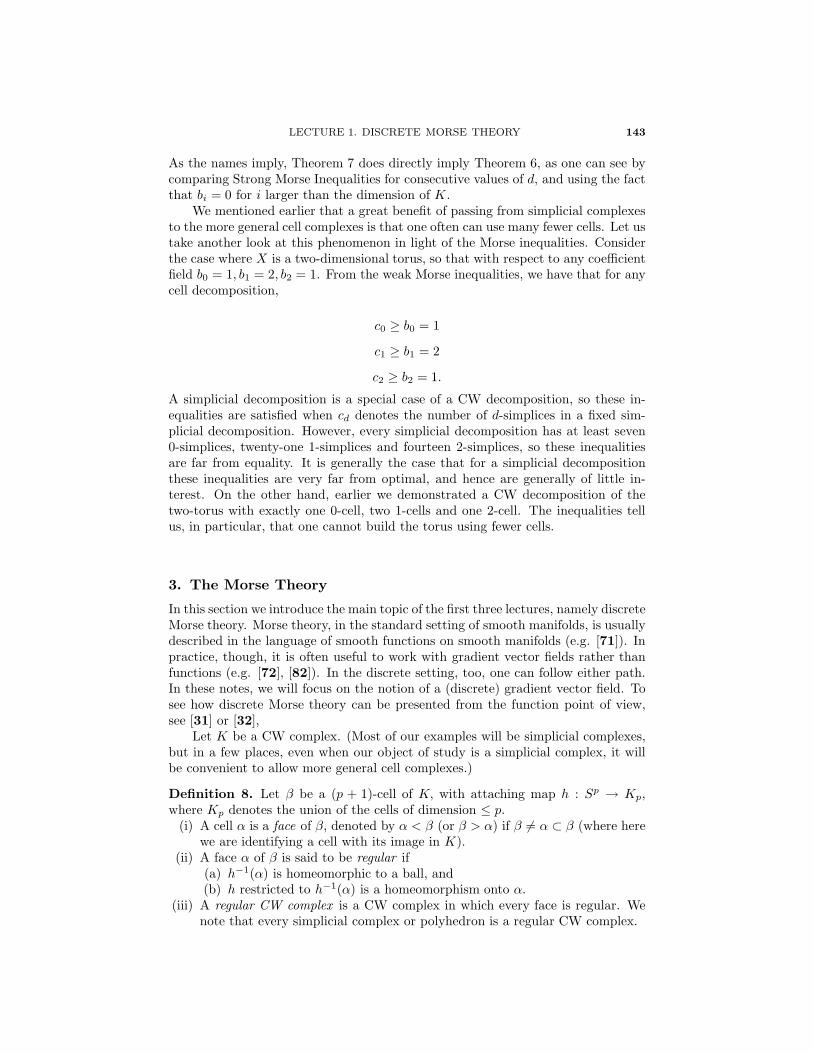
We mentioned earlier that a great benefit of passing from simplicial complexesto the more general cell complexes is that one often can use many fewer cells. Let ustake another look at this phenomenon in light of the Morse inequalities. Considerthe case where X is a two-dimensional torus, so that with respect to any coefficientfield b0 = 1, b1 = 2, b2 = 1. From the weak Morse inequalities, we have that for anycell decomposition,
c0 ≥ b0 = 1
c1 ≥ b1 = 2
c2 ≥ b2 = 1.
A simplicial decomposition is a special case of a CW decomposition, so these in-equalities are satisfied when cd denotes the number of d-simplices in a fixed sim-plicial decomposition. However, every simplicial decomposition has at least seven0-simplices, twenty-one 1-simplices and fourteen 2-simplices, so these inequalitiesare far from equality. It is generally the case that for a simplicial decompositionthese inequalities are very far from optimal, and hence are generally of little in-terest. On the other hand, earlier we demonstrated a CW decomposition of thetwo-torus with exactly one 0-cell, two 1-cells and one 2-cell. The inequalities tellus, in particular, that one cannot build the torus using fewer cells.
3. The Morse Theory
In this section we introduce the main topic of the first three lectures, namely discreteMorse theory. Morse theory, in the standard setting of smooth manifolds, is usuallydescribed in the language of smooth functions on smooth manifolds (e.g. [71]). Inpractice, though, it is often useful to work with gradient vector fields rather thanfunctions (e.g. [72], [82]). In the discrete setting, too, one can follow either path.In these notes, we will focus on the notion of a (discrete) gradient vector field. Tosee how discrete Morse theory can be presented from the function point of view,see [31] or [32],
Let K be a CW complex. (Most of our examples will be simplicial complexes,but in a few places, even when our object of study is a simplicial complex, it willbe convenient to allow more general cell complexes.)
Definition 8. Let β be a (p + 1)-cell of K, with attaching map h : Sp → Kp,where Kp denotes the union of the cells of dimension ≤ p.
(i) A cell α is a face of β, denoted by α < β (or β > α) if β �= α ⊂ β (where herewe are identifying a cell with its image in K).
(ii) A face α of β is said to be regular if(a) h−1(α) is homeomorphic to a ball, and(b) h restricted to h−1(α) is a homeomorphism onto α.
(iii) A regular CW complex is a CW complex in which every face is regular. Wenote that every simplicial complex or polyhedron is a regular CW complex.

144 R. FORMAN, COMB. DIFFERENTIAL TOPOLOGY AND GEOMETRY
Figure 3. A discrete vector field.
α0α1
α2 α3 α4 α5
Figure 4. A V -path.
Definition 9. A discrete vector field V on K is a collection of pairs {α(p) < β(p+1)}of cells of K such that each cell is in at most one pair of V, and such that if{α(p) < β(p+1)} is in V then α is a regular face of β.
We picture such vector fields by drawing, for each pair {α(p) < β(p+1)} ∈ V, anarrow whose tail lies in α and whose head lies in β (Figure 3). Such pairings werestudied in the case of a simplicial complex in [85] and [27] as a tool for investigatingthe possible f -vectors for a such complexes. Here we take a different point of view.Our first step is to introduce a special class of vector fields which will play the roleof gradient vector fields.
Definition 10.(1) Given a discrete vector field V on a cell complex K, a V -path is a sequence
of cells α0, α1, α2, . . . , αr such that for each i = 1, 2, . . . , r, either {αi−1 <αi} ∈ V or αi is a codimesion-one face of αi−1 and {αi < αi−1} /∈ V(Figure 4). We say such a path is a non-trivial closed path if r > 0 andα0 = αr.
(2) A discrete vector field V is a gradient vector field if there are no non-trivialclosed V -paths.
(3) If V is a gradient vector field on a cell complex K and α is a cell of Kwhich is not contained in any pair in V , then we say that α is a criticalcell of V .
The main theorem of discrete Morse theory is the following.
Theorem 11. Let K be a CW complex with a discrete gradient field V. Then K is(simple-)homotopy equivalent to a CW complex with precisely one cell of dimensionp for each critical cell of V of dimension p.
Before presenting the very simple proof, we will recall the notion of simple-homotopy. This idea was introduced by J.H.C. Whitehead in an effort to establisha combinatorial basis for homotopy theory. Let K be a CW complex.

LECTURE 1. DISCRETE MORSE THEORY 145
βα
K1 K2
Figure 5. An elementary collapse.
Definition 12. Let β be a (p + 1)-cell of K, and α a regular face of β. We saythat α is a free face of β if α is not the face of any other cell of K. (This impliesthat β is maximal, i.e. is not the face of any cell in K, and that dim(α) = p.)
If α is a free face of β then K − (int(α) ∪ int(β)) is a deformation retractof K. Such a deformation retract is called an elementary collapse (and in thecategory of simplicial complexes, an elementary simplicial collapse). See Figure 5.Simple-homotopy is the equivalence relation generated by elementary collapse.
We are now ready to present the proof of Theorem 11. (Many essentiallyequivalent proofs have appeared since the original proof in [32]. Here we presentthe very short proof that can be found in [59].)
Proof. Since V has no closed paths, we can find a cell α of K which has nopredecessors, i.e. such that there is no cell β such that β, α is a V -path. Thereare two possibilities, either (i) α is a maximal face, and is critical for V, or (ii) αis a free face of a cell β, and {α < β} ∈ V , see Figure 6. In case (i), K is theresult of attaching the cell α to K ′ = K − int(α). In case (ii), K collapses ontoK ′ = K − (int(α) ∪ int(β)). The proof now follows by induction. �
Combining Theorems 11, 6, and 7, and the fact that homotopy equivalentspaces have isomorphic homology, yields the following theorem.
Theorem 13. Let K be a simplicial complex with a discrete gradient vector field.Let mp denote the number of critical simplices of dimension p. Let F be any field,and bp = dimHp(K, F) the pth Betti number with respect to F. Then we have thefollowing relationships.
α
α
Figure 6. Two possibilities for a cell α with no predecessors.
146 R. FORMAN, COMB. DIFFERENTIAL TOPOLOGY AND GEOMETRY
empty
empty
1
1
1
2
2
2
3
3
3
3
12
12
12
13
13
23
23
123
123
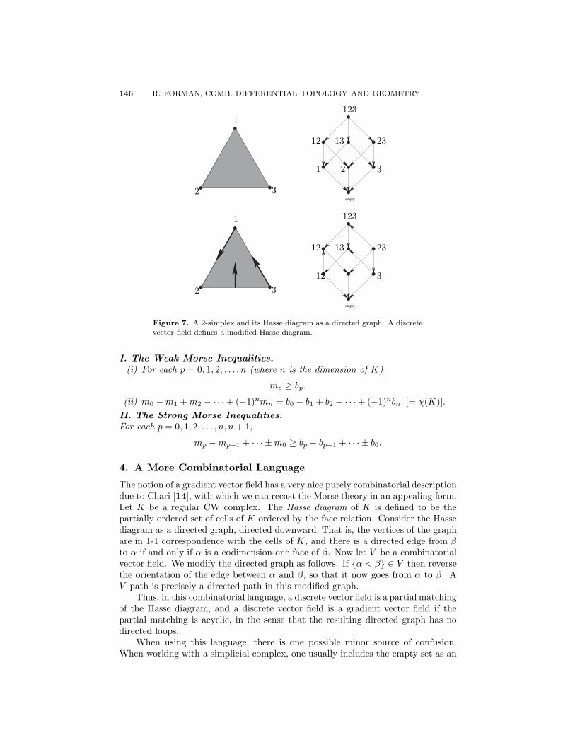
Figure 7. A 2-simplex and its Hasse diagram as a directed graph. A discretevector field defines a modified Hasse diagram.
I. The Weak Morse Inequalities.(i) For each p = 0, 1, 2, . . . , n (where n is the dimension of K)
mp ≥ bp.
(ii) m0 − m1 + m2 − · · · + (−1)nmn = b0 − b1 + b2 − · · · + (−1)nbn [= χ(K)].II. The Strong Morse Inequalities.For each p = 0, 1, 2, . . . , n, n + 1,
mp − mp−1 + · · · ± m0 ≥ bp − bp−1 + · · · ± b0.
4. A More Combinatorial Language
The notion of a gradient vector field has a very nice purely combinatorial descriptiondue to Chari [14], with which we can recast the Morse theory in an appealing form.Let K be a regular CW complex. The Hasse diagram of K is defined to be thepartially ordered set of cells of K ordered by the face relation. Consider the Hassediagram as a directed graph, directed downward. That is, the vertices of the graphare in 1-1 correspondence with the cells of K, and there is a directed edge from βto α if and only if α is a codimension-one face of β. Now let V be a combinatorialvector field. We modify the directed graph as follows. If {α < β} ∈ V then reversethe orientation of the edge between α and β, so that it now goes from α to β. AV -path is precisely a directed path in this modified graph.
Thus, in this combinatorial language, a discrete vector field is a partial matchingof the Hasse diagram, and a discrete vector field is a gradient vector field if thepartial matching is acyclic, in the sense that the resulting directed graph has nodirected loops.
When using this language, there is one possible minor source of confusion.When working with a simplicial complex, one usually includes the empty set as an

LECTURE 1. DISCRETE MORSE THEORY 147
1 3 1
11
2
22
2 3
33
(i) (ii)
e
e
t
Figure 8. (i) A triangulation of the projective plane. (ii) A discrete vectorfield on the projective plane.
element of the Hasse diagram (considered as a simplex of dimension -1), while wehave not considered the empty set previously. This issue will appear repeatedly inthese lectures.
5. Our First Example: The Real Projective Plane
Figure 8(i) shows a triangulation of the real projective plane P2. The vertices alongthe boundary with the same labels are to be identified, as are the edges whoseendpoints have the same labels. In Figure 8(ii) we illustrate a discrete vector fieldV on this simplicial complex. One can easily see that there are no closed V -paths(since all V -paths go to the boundary of the figure and there are no closed V -pathson the boundary), and hence is a gradient vector field. The only cells which areneither the head nor the tail of an arrow are the vertex label 1, the edge e, andthe triangle t. Thus, by Theorem 11, the projective plane is homotopy equivalentto a CW complex with exactly one 0-cell, one 1-cell and one 2-cell. (Of course, wealready knew this from our discussion of Example 3 in Section 2.)
This example gives rise to two potential concerns. The first is that from themain theorem we learn only a statement about “homotopy equivalence”. This issufficient if one is only interested in calculating homology or homotopy groups.However, one might be interested in determining the (PL-)homeomorphism type ofthe complex. This is possible, in some cases, using deep results of J. H. C. White-head. We revisit this topic briefly in the next section.
The second potential point of concern is that as we saw in Section 2 there arean infinite number of different homotopy types of CW complexes which can bebuilt from exactly one 0-cell, one 1-cell and one 2-cell. One might wonder if Morsetheory can give us any additional information as to how the cells are attached. Infact, one can deduce much of this information if one has enough information aboutthe gradient paths of the gradient vector field. This point is discussed further inSection 3 of Lecture 2, where we will return to this example of the triangulatedprojective plane.

148 R. FORMAN, COMB. DIFFERENTIAL TOPOLOGY AND GEOMETRY
6. Sphere Theorems
As mentioned in our discussion at the end of Section 5, one can sometimes usediscrete Morse theory to make statements about more than just the homotopy typeof the simplicial complex. One can sometimes classify the complex up to homeo-morphism or combinatorial equivalence. In this section we give some examples ofsuch arguments. An interesting application of these ideas is presented in the nextsection. So far, we have not placed any restrictions on the simplicial complexesunder consideration. The main idea of this section is that if our simplicial complexhas some additional structure, then one may be able to strengthen the conclusion.This idea rests on some very deep work of J. H. C. Whitehead [95].
A simplicial complex K is a combinatorial d-ball if K and the standard d-simplex σd have isomorphic subdivisions. A simplicial complex K is a combinatorial(d − 1)-sphere if K and σd have isomorphic subdivisions (where σd denotes theboundary of σd with its induced simplicial structure). A simplicial complex K isa combinatorial d-manifold with boundary if the link of every vertex is either acombinatorial (d − 1)-sphere or a combinatorial (d − 1)-ball. The following is aspecial case of the powerful main theorem of [95].
Theorem 14. Let K be a combinatorial d-manifold with boundary which simpli-cially collapses to a vertex. (That is, K can be a reduced to a vertex by a sequenceof elementary simplicial collapses.) Then K is a combinatorial d-ball.
With this theorem, and its generalizations, one can sometimes strengthen the con-clusion of Theorem 11 beyond homotopy equivalence. We present just one example.
Theorem 15. Let X be a combinatorial d-manifold with a discrete gradient vectorfield with exactly two critical simplices. Then X is a combinatorial d-sphere.
The proof is quite simple (given Theorem 14). The statement is trivial ford = 0, so we assume that d ≥ 1. Suppose that X is a combinatorial d-manifoldwith a discrete gradient vector field V with exactly two critical simplices. Let x0
be a vertex of X . If x0 is not critical, then {x0 < e} is an element of V , for someedge e. Let x1 be the other endpoint of e. Then x0, e, x1 is a V-path. If x1 isnot critical, we can follow the V -path to the next vertex x2, etc. Since there areonly a finite number of vertices, and there are no loops, we must eventually reacha critical vertex. We can run this argument in reverse for d-simplices. That is, ifα0 is a d-simplex, and α0 is not critical, then {β < α0} is an element of V for some(d−1)-simplex β. Let α1 denote the other d-simplex incident to β. Then α1, β, α0 isa V -path, and we can follow this path backwards until reaching a critical d-simplex.Thus, there must be precisely one critical vertex x, and one critical d-simplex α.Then X − α is a combinatorial d-manifold with boundary with a discrete gradientvector field with only a single critical simplex, namely the vertex x. It followsthat X − α collapses to x. Whitehead’s theorem now implies that X − α is acombinatorial d-ball, which implies that X is a combinatorial d-sphere.
7. Our Second Example
In this section we demonstrate some of the ideas of the previous sections with asimple example from algebra. Fix a positive integer n, and consider the following
LECTURE 1. DISCRETE MORSE THEORY 149
(((x0x1x2)x3)x4)
((x0x1x2)x3)
(x0x1x2)
x0 x1 x2 x3 x4
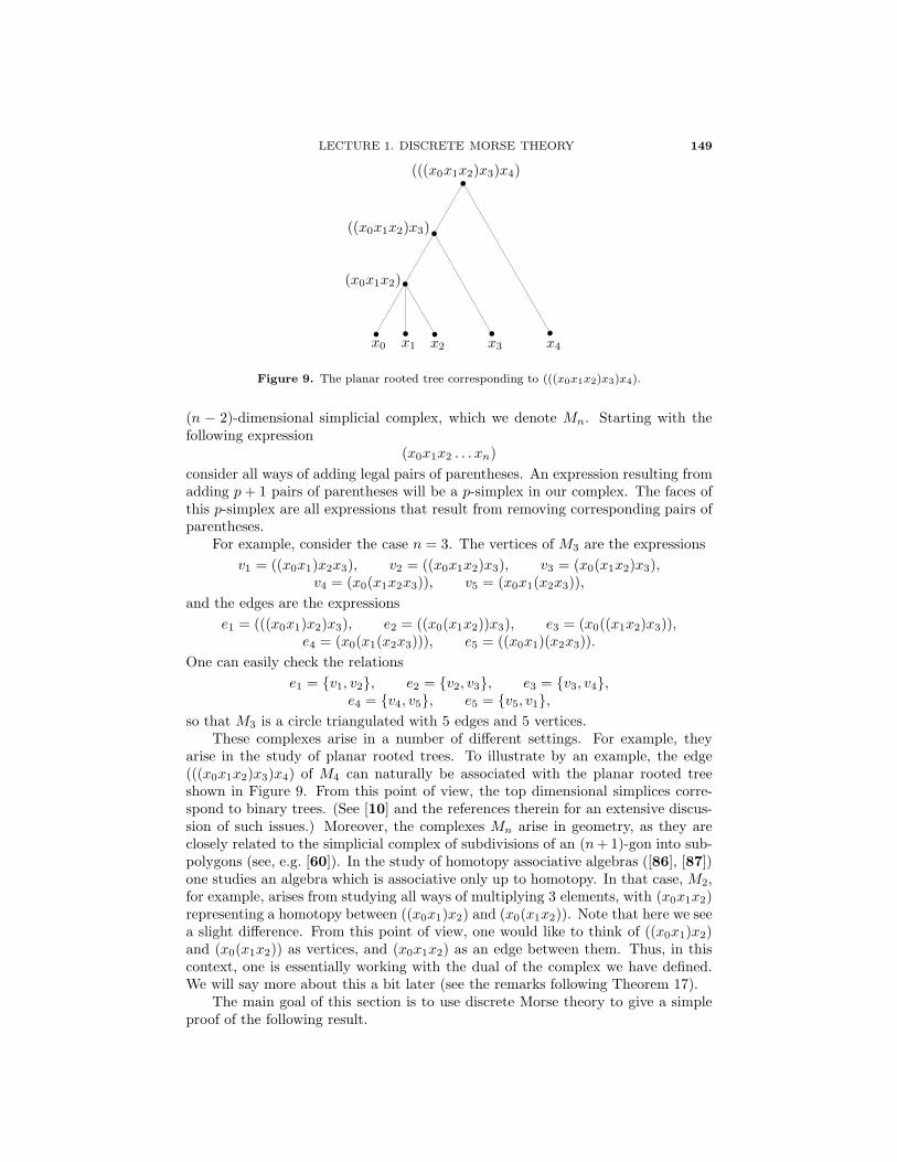
Figure 9. The planar rooted tree corresponding to (((x0x1x2)x3)x4).
(n − 2)-dimensional simplicial complex, which we denote Mn. Starting with thefollowing expression
(x0x1x2 . . . xn)consider all ways of adding legal pairs of parentheses. An expression resulting fromadding p + 1 pairs of parentheses will be a p-simplex in our complex. The faces ofthis p-simplex are all expressions that result from removing corresponding pairs ofparentheses.
For example, consider the case n = 3. The vertices of M3 are the expressionsv1 = ((x0x1)x2x3), v2 = ((x0x1x2)x3), v3 = (x0(x1x2)x3),
v4 = (x0(x1x2x3)), v5 = (x0x1(x2x3)),and the edges are the expressions
e1 = (((x0x1)x2)x3), e2 = ((x0(x1x2))x3), e3 = (x0((x1x2)x3)),e4 = (x0(x1(x2x3))), e5 = ((x0x1)(x2x3)).
One can easily check the relationse1 = {v1, v2}, e2 = {v2, v3}, e3 = {v3, v4},
e4 = {v4, v5}, e5 = {v5, v1},so that M3 is a circle triangulated with 5 edges and 5 vertices.
These complexes arise in a number of different settings. For example, theyarise in the study of planar rooted trees. To illustrate by an example, the edge(((x0x1x2)x3)x4) of M4 can naturally be associated with the planar rooted treeshown in Figure 9. From this point of view, the top dimensional simplices corre-spond to binary trees. (See [10] and the references therein for an extensive discus-sion of such issues.) Moreover, the complexes Mn arise in geometry, as they areclosely related to the simplicial complex of subdivisions of an (n + 1)-gon into sub-polygons (see, e.g. [60]). In the study of homotopy associative algebras ([86], [87])one studies an algebra which is associative only up to homotopy. In that case, M2,for example, arises from studying all ways of multiplying 3 elements, with (x0x1x2)representing a homotopy between ((x0x1)x2) and (x0(x1x2)). Note that here we seea slight difference. From this point of view, one would like to think of ((x0x1)x2)and (x0(x1x2)) as vertices, and (x0x1x2) as an edge between them. Thus, in thiscontext, one is essentially working with the dual of the complex we have defined.We will say more about this a bit later (see the remarks following Theorem 17).
The main goal of this section is to use discrete Morse theory to give a simpleproof of the following result.

150 R. FORMAN, COMB. DIFFERENTIAL TOPOLOGY AND GEOMETRY
Theorem 16. The complex Mn is homotopy equivalent to an (n − 2)-sphere.
This result is well known, and it is only our proof that is new. We will provethis theorem by showing that one can easily construct a discrete gradient vectorfield on Mn which has precisely two critical simplices, namely one critical vertexand one critical (n − 2)-simplex. The theorem then follows from Theorem 11. Infact, one can deduce more. We saw above that M3 is not just a homotopy circle, butrather it is an actual combinatorial circle. One can easily see that the link of everyvertex of Mn is isomorphic to a complex of the form Mp ∗ Mn−p (where ∗ denotesjoin). By induction, Mp and Mn−p are combinatorial spheres of dimension p−2 andn− p− 2, respectively, so the link is a combinatorial sphere of dimension n− 3 (seeProposition II.1 of [45]). Since the link of every vertex of Mn is a combinatorial(n− 3)-sphere, it follows that Mn is a combinatorial (n− 2)-manifold (see page 19of [45]). Therefore we can apply Theorem 6 to learn the following stronger result.
Theorem 17. The complex Mn is a combinatorial (n − 2)-sphere.
Before beginning our proof, we return to our earlier comments about the com-plex arising in the study of homotopy associative algebras. As remarked above, inthat case one considers what is essentially the dual of the complex Mn. However,there is a slight modification. Let M∗
n denote a combinatorial (n − 2)-sphere en-dowed with the cell decomposition which is dual to that of Mn. In Mn the trivialexpression (x0x1 . . . xn) corresponds to a simplex of dimension -1, i.e. the emptyset. In the dual setting, (x0x1, . . . xn) corresponds to a cell of dimension n − 1,whose boundary sphere is identified with all of M∗
n. Adding in this cell to formthe cone on M∗
n results in a complex, introduced in [86] (see also [87]) called theassociahedron (or Stasheff polytope), and which is often denoted An+1. Thus welearn
Corollary 18. The associahedron An+1 is a combinatorial (n − 1)-ball.
A proof of this appears in [86], by very different methods, and numerous alter-native proofs have also been presented. In fact, An+1 is a polytope ([60]). For moreabout the associahedron, from many points of view, one should certainly consultFomin and Reading’s wonderful lecture notes in this volume [30].
Let us now describe the construction of the desired gradient vector field V onMn. Let s be a simplex of Mn. Suppose that there is not a pair of parenthesisaround x0 and x1. If it is possible to legally add a pair of parentheses around x0 andx1 do so and call the resulting simplex t. We then add the pair {s ≺ t} to V . Forexample, in M4 the expression ((x0x1x2)(x3x4)) is paired with (((x0x1)x2)(x3x4)).After this step, the expressions which have not been paired with any other expres-sion are those that have at least one parenthesis between x0 and x1, and it is simpleto see that any such parenthesis must be a left parenthesis. There is one additionalunpaired expression, namely the expression s∗ = ((x0x1)x2x3 . . . xn). According toour rule, this should be paired with the original expression (x0, x1 . . . xn) with noadded parentheses, but this is not permitted.
If s is any expression other than s∗ that is currently unpaired, and a pair ofparentheses can legally be added around the elements x1 and x2, do so and callthe resulting simplex t. We then add the pair {s ≺ t} to V . After this step,the expressions which have not been paired with any other expression are s∗ andthose that have at least one left parenthesis between x0 and x1, and at least one left

LECTURE 1. DISCRETE MORSE THEORY 151
parenthesis between x1 and x2. Pair such an expression with the one resulting fromadding a pair of parentheses around x2 and x3 if possible. Continue this process aslong as possible. When it has terminated, the only expressions that have not beenpaired up with any other expression are s∗ and the one that has a left parenthesisbetween every consecutive pair x1 and xi+1 for i = 0, 1, . . . , n−1, i.e. the expressiont∗ = (x0(x1(x2(. . . (xn−2(xn−1xn)))) . . . ). Note that t∗ is an (n− 2)-simplex of thecomplex Mn.
This completes our construction of the vector field V . All that needs to bechecked is there are no closed V -paths. Denote by Vk the discrete vector field thathas been constructed after the kth step in the construction, i.e. after considera-tion of the pair xk−1, xk. It is simple to check that V1 has no closed orbits. Lets(p)0 , t
(p+1)0 , s
(p)1 denote a V -path. This requires that s0 and t0 be paired in V . Sup-
pose that s0 and t0 are paired in Vk The reader can check that this implies thateither s1 is the head of an arrow in Vk (and hence the V -path cannot be continued)or s1 is paired in Vk−1. Thus, by induction, there can be no closed V -paths.
8. Exercises for Lecture 1
(1) (a) Prove the strong Morse inequalities. That is, suppose that
V : 0 → Vn∂n→ Vn−1
∂n−1→ Vn−2∂n−2→ · · · ∂1→ V0 → 0
is a differential complex (i.e. ∂i+1 ◦ ∂i = 0 for all i). Let mi de-note the dimension of Vi, and bi the dimension of the ith homology(=Ker(∂i)/ Im(∂i+1)). Prove that for each i
mi − mi−1 + mi−2 − · · · ± m0 ≥ bi − bi−1 + bi−2 − · · · ± b0.
Make sure you see how these inequalities imply the Weak MorseInequalities.
(b) Now prove the converse of the Morse inequalities. That is, supposethat we are given finite lists of nonnegative integers m0, . . . , mn, andb0, . . . , bn which satisfy the above inequality for each i. Prove thatthere is a complex V as above with mi = dim(Vi) for each i, and suchthat bi is the dimension of the ith homology. [This shows that onecannot deduce anything stronger than the strong Morse inequalitiesusing only the abstract existence of a complex which calculates thedesired homology.]
(2) Prove that every triangulated disc is collapsible (i.e. collapses to a vertex).(3) Triangulate a torus (more precisely, construct a simplicial complex which
is homeomorphic to the torus) and find a discrete gradient field on theresulting simplicial complex with as few critical simplices as possible.
(4) Prove that every triangulated surface has a perfect gradient vector field.That is, let M be a connected simplicial complex which is homeomorphicto a compact surface. Prove that there is a gradient vector field on Mwith precisely 1 critical vertex, 1 critical 2-simplex, and g critical edges,where g denotes the genus of M. (Hint: Use the Morse inequalities to seethat it is sufficient to find a discrete gradient vector field with exactly onecritical vertex, and exactly one critical triangle.)
(5) One can also present discrete Morse theory using the language of functions,rather than gradient vector fields. Let K be a finite simplicial complex.

152 R. FORMAN, COMB. DIFFERENTIAL TOPOLOGY AND GEOMETRY
A function f : K → R (i.e. f assigns a single real number to each simplex)is called a discrete Morse function if for each p-simplex α
#{β(p+1) > α s.t. f(β) ≤ f(α)} ≤ 1and
#{γ(p−1) < α s.t. f(γ) ≥ f(α)} ≤ 1.
Given such a function f, define a set of pairs Vf by declaring that {α <β} ∈ Vf if α is a codimension-one face of β and f(β) ≤ f(α).(a) Show that Vf is actually a discrete vector field (i.e. that each simplex
is contained in at most one pair in V ).(b) Show that Vf is a gradient vector field.(c) Show that every gradient vector field arises in this way. That is, if
V is a gradient vector field, then there is a discrete Morse function fsuch that V = Vf .
LECTURE 2Discrete Morse Theory, continued
1. Suspensions and Discrete Morse Theory
Let K be a simplicial complex, and let x and y be two points not in K. Then thesuspension of K is defined to be the join of K and the set {x, y}. More geometrically,embed K in some Rd, and embed Rd in Rd+1 by adding a final coordinate. Letx be the point (0, . . . , 0, 1) and y the point (0, . . . , 0,−1). Then the suspension ofK is the union of all of the closed line segments connecting x to a point in K andall of the closed line segments connecting the point y to a point in K. This spacecomes with a natural simplicial decomposition induced from that of K.
Let S be a simplex, and M a nonempty proper subcomplex of S. There aretwo interesting topological spaces to consider in this setting. One is M itself, andthe other is S/M , the result of identifying all of the points in M to a single point.While S/M is not a simplicial complex, it does have a canonical cell decompositiongiving S/M the structure of a CW complex. Moreover, if α < β are two faces of Swhich are not in M, and α∗ and β∗ are their images in S/M, then α∗ < β∗, andmoreover, α∗ is a regular face of β∗.
In fact, the two spaces M and S/M are closely related, and one can deduceessentially the entire topological structure of either one from a knowledge of theother. More precisely, we have the following statement.
Theorem 19. S/M is homotopy equivalent to the suspension of M .
Of particular interest to us is the following result.
Corollary 20. For any p, Hp+1(S/M, Z) ∼= Hp(M, Z).
These results are not hard to prove using standard methods, but we present adiscrete Morse theory proof of Corollary 20, as the technique (more than the result)will prove useful later (see the next section). In fact, a more careful analysis of thisproof allows one to deduce Theorem 19, but we will leave that to the reader. Ourapproach is to simultaneously construct gradient vector fields U and V on M andS/M , respectively. Let v be any vertex of M . If α is a nonempty simplex of Mwhich does not contain v and which has the property that v ∗ α is also in M , then
153

154 R. FORMAN, COMB. DIFFERENTIAL TOPOLOGY AND GEOMETRY
pair α with v ∗ α. Let U1 denote this collection of pairs. That is
U1 = {{α < v ∗ α} s.t. ∅ �= α and v ∗ α ⊂ M}.It is a simple observation that U1 is a gradient vector field. Similarly, define agradient vector field V1 on S/M by setting
V1 = {{α < v ∗ α} s.t. ∅ �= α and α � M}.(We are now identifying a simplex α in S, α � M , with its image in S/M.) Thesimplices of M which are critical for U1 are the vertex v and any nonempty simplex αof M with the property that v ∗ α � M . Let CU denote this collection of criticalsimplices of U1. The cells of S/M which are critical for V1 are the special 0-cell min S/M resulting from identifying all of the points in M , along with any nonemptysimplex β � M which has the property that v ∈ β, and β − v ⊂ M . Let CV denotethis collection of critical simplices of V1. We observe that there is a canonicalidentification of the elements of CU with those of CV . Namely, identify v ∈ Mwith m ∈ S/M, and identify α with v ∗ α whenever α ⊂ M and v ∗ α � M. LetU denote any vector field on M which is an extension of U1, and let U2 = U − U1
(so that U2 consists of pairs of elements in CU ). Define V2 = {{v ∗ α < v ∗ β} s.t.{α < β} ∈ U2}, and let V = V1 ∪ V2.
Lemma 21.(i) Let A = α1, α2, α3, . . . , αk be a sequence of elements in CU , and let B =
v ∗ α1, v ∗ α2, v ∗ α3, . . . , v ∗ αk be the corresponding sequence of elements inCV . Then A is a U -path if and only if B is a V -path
(ii) V is a gradient vector field if and only if U is.
Proof. Part (i) follows immediately from the construction of V . To prove part (ii)let M ′ = M − CU , and S′ = S/M − CV . (These are the cells that are paired in U1
and V1, respectively.) It is easy to see that any U -path that begins in M ′ staysin M ′, and hence is a U1-path. Since U1 is a gradient vector field, none of theseU -paths are closed. Similarly, any V -path that begins in S′ stays in S′, and none ofthese are closed. Hence any closed U -path must lie entirely in CU . Now the resultfollows from part (i). �
If U is a vector field on M which contains U1, we say that U collapses towardsv. If V is a vector field on S/M which contains V1, then we say that V collapsestowards v∗. Then Lemma 21 leads to the following result.
Theorem 22. For any vertex v of M , there is a canonical identification of gradi-ent vector fields of M which collapse towards v, and those of S/M which collapsetowards v∗. If U is a gradient vector field on M which collapses towards v, and Vis the corresponding gradient vector field on S/M, then v is critical for U, and mis critical for V. For every additional critical simplex α of U, v ∗α is critical for V,and every critical cell of V arises in this manner.
In Section 3 we will introduce the Morse complex, a method of calculating thehomology of a cell complex exactly using a knowledge of the critical cells and thegradient paths. The preceeding discussion is sufficient, modulo some minor detailswhich can be supplied by the reader, to deduce that the Morse complex for therelative pair (M, v), which computes the reduced homology of M , is isomorphicto the Morse complex of the relative pair (S/M, m), which computes the reduced

LECTURE 2. DISCRETE MORSE THEORY, CONTINUED 155
homology of S/M , with the isomporphism shifting all degrees up by 1. This sufficesto prove Theorem 20. A more careful consideration of the implications of Theorem22 yields Theorem 19.
2. Monotone Graph Properties
A number of fascinating simplicial complexes arise from the study of monotonegraph properties. Let Kn denote the complete graph on n vertices, and suppose wehave label the vertices 1,2,. . . ,n. Let Gn denote the set of spanning subgraphs ofKn, that is, the subgraphs of Kn that contain all n vertices. (Elements of Gn arepermitted to be disconnected and to have isolated vertices.) A subset P ⊂ Gn iscalled a graph property of graphs with n vertices if inclusion in P only depends onthe isomorphism type of the graph. That is, P is a graph property if for all pairsof graphs G1, G2 ∈ Gn, if G1 and G2 are isomorphic (ignoring the labelings on thevertices) then G1 ∈ P if and only if G2 ∈ P . A graph property P of graphs withn vertices is said to be monotone decreasing if for any graphs G1 ⊂ G2 ∈ Gn, ifG2 ∈ P then G1 ∈ P .
Monotone decreasing properties abound in the study of graph theory. Here aresome typical examples: graphs having no more than k edges (for any fixed k), graphssuch that the degree of every vertex is less that δ (for any fixed δ), graphs whichare not connected, graphs which are not i-connected (for any fixed i), graphs whichdo not have a Hamiltonian cycle, graphs which do not contain a minor isomorphicto H (for any fixed graph H), graphs which are r-colorable (for any fixed r), andbipartite graphs.
Any monotone decreasing graph property P gives rise to a simplicial complex Kwhere the d-simplices of K are the graphs G ∈ P which have d + 1 edges. Inparticular, if G is a d-simplex in K, then the faces of G are all of the nontrivialspanning subgraphs of G (the monotonicity of P implies that each of these graphs isin K). Said in another way, if P is nonempty, then the vertices of K are the edges ofKn (more precisely, the spanning subgraphs of Kn which include all n vertices andprecisely one edge), and a collection of vertices in K span a simplex if the spanningsubgraph of Kn consisting of all edges which correspond to these vertices lies in P .
The simplicial complexes induced by many of the above-mentioned monotonedecreasing graph properties have been studied using the techniques of these notes.See for example [14], [25], [52], [53], [65], and [79]. These papers contain somebeautiful mathematics in which the authors construct “by hand” explicit discretegradient vector fields, along the way illuminating some of the intricate finer struc-tures of the graph properties.
Some monotone graph properties have recently been the focus of intense interestbecause of their relation to knot theory. Unfortunately this is probably not a goodtime for an in depth discussion of this fascinating topic. We will mention onlythat Vassiliev has shown how one can derive finite type knot invariants from thestudy of the space of “singular knots” (i.e. maps from S1 to R3 which are notembeddings). The homology of the simplicial complexes of disconnected and not-2-connected graphs show up in his spectral sequence calculation of the homology ofthis space. This is explained in [93], where Vassiliev derives the homotopy type ofthe complex of disconnected graphs. In [92] and [6], the topology of the space of
156 R. FORMAN, COMB. DIFFERENTIAL TOPOLOGY AND GEOMETRY
1 2
connectedconnected
component component
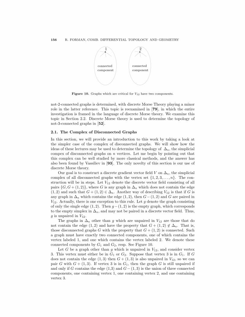
Figure 10. Graphs which are critical for V12 have two components.
not-2-connected graphs is determined, with discrete Morse Theory playing a minorrole in the latter reference. This topic is reexamined in [79], in which the entireinvestigation is framed in the language of discrete Morse theory. We examine thistopic in Section 2.2. Discrete Morse theory is used to determine the topology ofnot-3-connected graphs in [52].
2.1. The Complex of Disconnected Graphs
In this section, we will provide an introduction to this work by taking a look atthe simpler case of the complex of disconnected graphs. We will show how theideas of these lectures may be used to determine the topology of Δn, the simplicialcompex of disconnected graphs on n vertices. Let me begin by pointing out thatthis complex can be well studied by more classical methods, and the answer hasalso been found by Vassiliev in [93]. The only novelty of this section is our use ofdiscrete Morse theory.
Our goal is to construct a discrete gradient vector field V on Δn, the simplicialcomplex of all disconnected graphs with the vertex set {1, 2, 3, . . . , n}. The con-struction will be in steps. Let V12 denote the discrete vector field consisting of allpairs {G, G + (1, 2)}, where G is any graph in Δn which does not contain the edge(1, 2) and such that G + (1, 2) ∈ Δn. Another way of describing V12 is that if G isany graph in Δn which contains the edge (1, 2), then G− (1, 2) and G are paired inV12. Actually, there is one exception to this rule. Let g denote the graph consistingof only the single edge (1, 2). Then g−(1, 2) is the empty graph, which correspondsto the empty simplex in Δn, and may not be paired in a discrete vector field. Thus,g is unpaired in V12.
The graphs in Δn other than g which are unpaired in V12 are those that donot contain the edge (1, 2) and have the property that G + (1, 2) �∈ Δn. That is,those disconnected graphs G with the property that G + (1, 2) is connected. Sucha graph must have exactly two connected components, one of which contains thevertex labeled 1, and one which contains the vertex labeled 2. We denote theseconnected components by G1 and G2, resp. See Figure 10.
Let G be a graph other than g which is unpaired in V12, and consider vertex3. This vertex must either be in G1 or G2. Suppose that vertex 3 is in G1. If Gdoes not contain the edge (1, 3) then G + (1, 3) is also unpaired in V12, so we canpair G with G + (1, 3). If vertex 3 is in G1, then the graph G is still unpaired ifand only if G contains the edge (1,3) and G− (1, 3) is the union of three connectedcomponents, one containing vertex 1, one containing vertex 2, and one containingvertex 3.

LECTURE 2. DISCRETE MORSE THEORY, CONTINUED 157
Similarly, if vertex 3 is in G2 and G does not contain the edge (2, 3), then pairG with G + (2, 3). Let V3 denote the resulting discrete vector field.
The unpaired graphs in V3 are g and those that either contain the edge (1,3)and have the property that G− (1, 3) is the union of three connected components,one containing vertex 1, one containing vertex 2, and one containing vertex 3, orcontain the edge (2,3) and have the property that G − (2, 3) is the union of threeconnected components, one containing vertex 1, one containing vertex 2, and onecontaining vertex 3. We illustrate these graphs in Figure 11. The circles in thisfigure indicate connected subgraphs.
Now consider the location of the vertex label 4, and pair any graph G whichis unpaired in V3 with G + (1, 4), G + (2, 4), or G + (3, 4) if possible (at most oneof these graphs is unpaired in V3). Call the resulting discrete vector field V4. Wecontinue in this fashion, considering in turn the vertices label 5, 6, . . . , n. Let Vi
denote the discrete vector field that has been constructed after the considerationof vertex i, and V = Vn the final discrete vector field. When we are done theonly unpaired graphs in V will be g and those graphs that are the union of twoconnected trees, one containing the vertex 1 and one containing the vertex 2. Inaddition, both trees have the property that the vertex labels are increasing alongevery ray starting from the vertex 1 or the vertex 2. There are precisely (n−1)! suchgraphs, and they each have n−2 edges, and hence correspond to an (n−3)-simplexin Δn.
It remains to see that the discrete vector field V is a gradient vector field,i.e. that there are no closed V -paths. We first check that V12 is a gradient vectorfield. Let γ = α
(p)0 , β
(p+1)0 , α
(p)1 denote a V12-path. Then α0 must be the “tail of an
arrow”, i.e. the smaller graph of some pair in V12, with β0 being the head of thearrow, i.e. β0 = α0 + (1, 2). The simplex α1 is a codimension-one face of β0 otherthan α0. Thus, α1 corresponds to a graph of the form α0 + (1, 2)− e, where e is anedge of α0 other than (1,2). Since α1 contains the edge (1, 2) it is the “head of anarrow” in V12, i.e. the larger graph of some pair in V12, which implies that γ cannotbe continued to a longer V12-path. This certainly implies that there are no closedV12-paths.
1 1 22
33
connected
connected
connectedconnected
connected
connected
component
componentcomponent
component
component component
Figure 11. The two types of graphs which are critical for V3.
158 R. FORMAN, COMB. DIFFERENTIAL TOPOLOGY AND GEOMETRY
(i)
1
2v3 v4 v5 vn· · ·
· · ·
(ii)
1
2v3 v4 v5 vn· · ·
· · ·
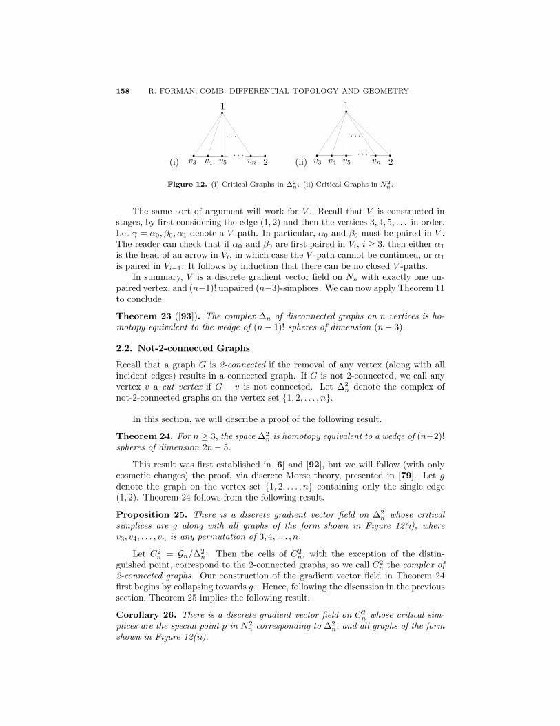
Figure 12. (i) Critical Graphs in Δ2n. (ii) Critical Graphs in N2
n.
The same sort of argument will work for V . Recall that V is constructed instages, by first considering the edge (1, 2) and then the vertices 3, 4, 5, . . . in order.Let γ = α0, β0, α1 denote a V -path. In particular, α0 and β0 must be paired in V .The reader can check that if α0 and β0 are first paired in Vi, i ≥ 3, then either α1
is the head of an arrow in Vi, in which case the V -path cannot be continued, or α1
is paired in Vi−1. It follows by induction that there can be no closed V -paths.In summary, V is a discrete gradient vector field on Nn with exactly one un-
paired vertex, and (n−1)! unpaired (n−3)-simplices. We can now apply Theorem 11to conclude
Theorem 23 ([93]). The complex Δn of disconnected graphs on n vertices is ho-motopy equivalent to the wedge of (n − 1)! spheres of dimension (n − 3).
2.2. Not-2-connected Graphs
Recall that a graph G is 2-connected if the removal of any vertex (along with allincident edges) results in a connected graph. If G is not 2-connected, we call anyvertex v a cut vertex if G − v is not connected. Let Δ2
n denote the complex ofnot-2-connected graphs on the vertex set {1, 2, . . . , n}.
In this section, we will describe a proof of the following result.
Theorem 24. For n ≥ 3, the space Δ2n is homotopy equivalent to a wedge of (n−2)!
spheres of dimension 2n− 5.
This result was first established in [6] and [92], but we will follow (with onlycosmetic changes) the proof, via discrete Morse theory, presented in [79]. Let gdenote the graph on the vertex set {1, 2, . . . , n} containing only the single edge(1, 2). Theorem 24 follows from the following result.
Proposition 25. There is a discrete gradient vector field on Δ2n whose critical
simplices are g along with all graphs of the form shown in Figure 12(i), wherev3, v4, . . . , vn is any permutation of 3, 4, . . . , n.
Let C2n = Gn/Δ2
n. Then the cells of C2n, with the exception of the distin-
guished point, correspond to the 2-connected graphs, so we call C2n the complex of
2-connected graphs. Our construction of the gradient vector field in Theorem 24first begins by collapsing towards g. Hence, following the discussion in the previoussection, Theorem 25 implies the following result.
Corollary 26. There is a discrete gradient vector field on C2n whose critical sim-
plices are the special point p in N2n corresponding to Δ2
n, and all graphs of the formshown in Figure 12(ii).

LECTURE 2. DISCRETE MORSE THEORY, CONTINUED 159
Proposition 25 and Corollary 26 will be proved simultaneously, inductively onn. For n = 3, the set G3 of graphs on the vertex set {1, 2, 3}, is a 2-dimensionalsimplex on the vertex set consisting of the 3 possible edges {(1, 2), (2, 3), (1, 3)}.The only graph on 3 vertices which is 2-connected is K3, which corresponds to themaximal face of G3. That is, Δ2
3 is a circle, and the gradient vector field whichcollapses towards (1, 2), has critical vertex {[1, 2]} and critical edge {(2, 3), (1, 3)}.The space C2
n, resulting from collapsing Δ23 to a point, is a 2-sphere consisting of
the point p and the 2-cell K3. The only possible gradient vector field in C2n is empty
so that both cells are critical. These gradient vector fields satisfy the conclusionsof Proposition 25 and Corollary 26.
Now let us begin to construct a gradient vector field on Δ2n for general n
(assuming the construction of such a gradient vector field on C2n−1). First, we
collapse towards g. That is, set
V1 = {{G − (1, 2), G}}where G ranges over all graphs which are not 2-connected and contain theedge (1, 2). Let M1 denote the graphs which remain unpaired. Then M1 con-sists of all graphs G which are not 2-connected, and do not contain the edge (1, 2),and have the property that G + (1, 2) is 2-connected.
To describe the next step in our construction of V, we must take a closer look atsuch graphs. Such a graph G must be connected (as otherwise G+(1, 2) cannot be2-connected). Let us now recall the basic structure of connected, not-2-connectedgraphs. Let H be such a graph, and let H1 be an induced 2-connected subgraphwhich is maximal among all induced 2-connected subgraphs. (A subgraph H ofa graph G is said to be induced if H contains all edges of G which connect twovertices of H .) Let H2 denote another maximal induced 2-connected subgraph.Then H1 ∩ H2 can contain at most one vertex (as otherwise the induced graph onV (H1) ∪ V (H2) would be 2-connected, and larger than H1 and H2). If H1 ∩ H2
contains a vertex, then that vertex must be a cut vertex of H. Conversely, anycut vertex of H is of the form H1 ∩ H2 for some maximal induced 2-connectedsubgraphs H1 and H2. Now let H(2) denote the graph whose vertices are themaximal induced 2-connected subgraphs of H, with the property that if H1 and H2
are maximal induced 2-connected subgraphs of H, then the corresponding verticesof H(2) are adjacent if and only if H1 ∩ H2 is not empty. Clearly every vertex ofH is contained in some maximal induced 2-connected subgraph of H. Moreover,H is not 2-connected, which implies that H(2) has at least 2 vertices. Lastly, weobserve that every minimal loop in H is contained in some maximal induced 2-connected subgraph of H, and hence appears as a vertex in H(2), from which onecan deduce that H(2) has no loops, i.e. H(2) is a tree. Now let G be a connected,not-2-connected graph with the property that G + (1, 2) is 2-connected. Note thatvertices 1 and 2 cannot be contained in the same maximal induced 2-connectedsubgraph of G, as otherwise the blocks of G + (1, 2) would be the same as thoseof G, and hence G + (1, 2) would not be 2-connected. Let G1 denote the maximalinduced 2-connected subgraph of G that contains the vertex 1, and G2 the maximalinduced 2-connected subgraph of G that contains the vertex 2. It is easy to see thatG1 �= G2 (as otherwise G + (1, 2) cannot be 2-connected). In fact, the followingresult is easily established.
Lemma 27. With all notation as above, G(2) is a path from G1 to G2.

160 R. FORMAN, COMB. DIFFERENTIAL TOPOLOGY AND GEOMETRY
Now let G3 denote the induced maximal 2-connected subgraph which is adjacentto G1 in G(2), and let v(G) be the vertex G1 ∩ G3. It is clear that v(G) �= 2.Moreover, if v(G) = 1 then vertex 1 would be a cut vertex of G+(1, 2), contradictingthe assumption that G + (1, 2) is 2-connected. Therefore v(G) /∈ {1, 2}. SupposeG ∈ M1 and (v(G), 2) /∈ G. It is easy to see that v(G) is a cut vertex of G+(v(G), 2),and hence G + (v(G), 2) is not 2-connected. Moreover, [G + (v(G), 2)] + (1, 2) =[G + (1, 2)] + (v(G), 2) is 2-connected (since [G + (1, 2)] is), so G + (v(G), 2) ∈ M1.Now define
V2 = { {G, G + (v(G), 2)}}where G ranges over all graphs in M1 which do not contain (v(G), 2).
Let M2 contain the graphs which are not paired in V1 or V2. Then M2 consistsof those graphs G in M1 which contain (v(G), 2), and which have the property thatG − (v(G), 2) /∈ M1. First note that since (v(G), 2) ∈ G, v(G) and 2 are containedin an induced 2-connected subgraph, which implies that v(G) ∈ G2, and hence G1
and G2 are connected in G(2). From the previous lemma, we learn that G(2) mustconsist of only the two vertices G1 and G2 and the edge between them. The onlyway G − (v(G), 2) could fail to be in M1 is if G − (v(G), 2) failed to be connected.This can happen only if G2 − (v(G), 2) is not connected. However, since G2 is 2-connected, this can happen only if G2 consists entirely of the vertices 2 and v(G) andthe edge between them. Thus, the graphs G in M2 are precisely those that can beconstructed by taking a 2-connected graph G1 on the vertex set {1, 2, . . . , n}−{2},adding the vertex 2, and adding the edge (i, 2) for some i /∈ {1, 2} (in which casev(G) = i).
Let M2(i), i = 3, 4, . . . , n, denote those graphs G in M2 with v(G) = i. ThenM2 is the disjoint union of the M2(i)’s. Each M2(i) can be canonically identifiedwith the complex Γ of 2-connected graphs on the n − 1 vertices {1, 3, 4, . . . , n}.By induction, there is a gradient vector field on Γ with precisely (n − 3)! criticalsimplices of dimension 2(n − 1) − 5. = 2n − 7. Using the identification, we get agradient vector field V3(i) on M2(i) with (n − 3)! critical simplices of dimension2n− 6. Let
V = V1 ∪ V2 ∪ (∪ni=3V3(i)).
Since there are n − 2 such M2(i)’s, the total number of unmatched simplices in Vis (n − 2)(n − 3)! = (n − 2)!, each of dimension 2n − 6. The theorem now followsonce we know that V is a gradient vector field.
Lemma 28. The vector field V constructed above is a gradient vector field.
The proof is left as a (rather non-trivial) exercise.It is, in fact, quite easy to identify more explicitly the critical simplices in the
above gradient vector field. To find the critical graphs in M2(i), i = 3, 4, . . . , n,we take the critical graphs in the complex of 2-connected graphs on the vertex set{1, 3, 4, . . . , n} with respect to some optimal gradient vector field add the vertex 2and the edge (i, 2) for some i = 3, 4, . . . , n. Fixing i, identify {1, 3, 4, . . . , n} with{1, 2, . . . , n−1} via a correspondence that identifies 1 with 1, and identifies i with 2.By induction, there is a gradient vector field on the 2-connected graphs on the vertexset {1, 2, . . . , n − 1} whose critical simplices have the form shown in Figure 12(ii).Using the identification, we get a gradient vector field on 2-connected graphs on the

LECTURE 2. DISCRETE MORSE THEORY, CONTINUED 161
1
v3 v4 vi−1 vi+1 vn i· · · · · ·
· · ·· · ·
Figure 13. Critical 2-connected graphs on the vertex set {1, 2, 3, . . . , n}.
vertex set {1, 3, 4, . . . , n} whose critical simplices are of the form shown in Figure 13(where v3, v4, . . . , vi−1, vi+1, . . . , vn is any permutation of 3, 4, . . . , i−1, i+1, . . . , n).
Adding a vertex 2 to each such graph, and adding an edge between vertex i andvertex 2 yields the desired collection of graphs shown in Figure 12(i). Corollary 26now follows from Theorem 22.
2.3. Some further thoughts
The reader may wonder why we stopped with not-2-connected graphs. In fact, withquite a bit of hard work, it is possible to go further. In [52] J. Jonsson used discreteMorse theory to prove the following result.
Theorem 29. The simplicial complex Δ3n of not-3-connected graphs is homotopy
equivalent to a wedge of (n − 3) · (n − 2)!/2 spheres of dimension (2n − 1).
Many of the gradient vector fields presented in these notes, including the twoexamples in this section, follow a similar pattern, in that one constructs the gradientvector field in several stages, following distinct rules for each stage. In this way, auser of discrete Morse theory generally discovers the following useful observation,which appeared implicitly earlier, but seems to have been first explicitly stated in[52] and [50].
Lemma 30. Let K = �i∈IKi be a partition of the faces of K, where I is somepartially ordered set. Suppose that for every i ∈ I, ∪j≤iKj is a subcomplex of K.Now suppose we have a discrete vector field Vi on each Ki (that is, a partial pairingof the simplices in Ki) with the property that there are no closed Vi-paths in Ki.Then V = ∪i∈IVi is a gradient vector field on K.
3. The Morse Complex
In this section we will see how more precise knowledge of the gradient vector fieldon a simplicial complex K allows one to strengthen the conclusions of the maintheorems of discrete Morse theory. In particular, rather than just knowing thenumber of cells in a CW decomposition for K, one can calculate the homologyexactly.
Let K be a simplicial complex with a gradient vector field V . In keeping withthe standard terminology in the smooth category, we will refer to V -paths (seeSection 3) as gradient paths. Let Cp(K, Z) denote the space of simplicial p-chains,and Mp ⊆ Cp(K, Z) the span of the critical p-simplices of V . We refer to M∗ asthe space of Morse chains. If we let mp denote the number of critical p-simplices,then we obviously have
Mp∼= Zmp .

162 R. FORMAN, COMB. DIFFERENTIAL TOPOLOGY AND GEOMETRY
Since homotopy equivalent spaces have isomorphic homology, the following theoremfollows from Theorems 11 and 5.
Theorem 31. There are boundary maps ∂d : Md → Md−1, for each d, so that
∂d−1 ◦ ∂d = 0
and such that the resulting differential complex
(3) 0 −−−−→ Mn∂n−−−−→ . . .
∂1−−−−→ M0 −−−−→ 0calculates the homology of K. That is, if we define
Hd(M, ∂) =Ker(∂d)Im(∂d+1)
then for each d
Hd(M, ∂) ∼= Hd(K, Z).
In fact, this statement is equivalent to the Strong Morse inequalities (see Exer-cise 1 of Lecture 1). The main goal of this section is to present an explicit formulafor the boundary operator ∂. This requires a closer look at the notion of a gradientpath. Let β be a critical (p + 1) simplex, and and α a critical p-simplex. Then itis easy to check that any gradient-path from β to α has the form
β = β(p+1)0 , α
(p)1 , β
(p+1)1 , α
(p)2 , . . . , β(p+1)
r , α(p)r+1 = α
such that for each i = 0, 1, 2, . . . , r , {αi+1 < βi+1} ∈ V, and αi+1 < βi, but{αi+1 < βi} /∈ V. In Figure 14 we show a single gradient path from the boundary ofa critical 2-simplex β to a critical edge α, where the arrows pointing from an edgeto a 2-cell indicate the gradient vector field V .
Given a gradient path as shown in Figure 14, an orientation on β induces anorientation on α. We will not state the precise definition here. The idea is thatone “slides” the orientation from β along the gradient path to α. For example, forthe gradient path shown in Figure 14, the indicated orientation on β induces theindicated orientation on α.
We are now ready to state the desired formula.
Theorem 32. Choose an orientation for each simplex. Then for any critical (p+1)-simplex β set
(4) ∂β =∑
critical α(p)
cα,βα
wherecα,β =
∑γ∈Γ(β,α)
m(γ)
where Γ(β, α) is the set of gradient paths which go from β to α. The multiplicitym(γ) of any gradient path γ is equal to ±1, depending on whether, given γ, theorientation on β induces the chosen orientation on α, or the opposite orientation.With this differential, the complex (3) computes the homology of K.
We refer to the complex (3) with the differential (4) as the Morse complex (itgoes by many different names in the literature). An extensive study of the Morsecomplex in the smooth category appears in [78]. In is section, we have focusedour attention on simplicial complexes. However, it is worth noting that this entire

LECTURE 2. DISCRETE MORSE THEORY, CONTINUED 163
αβ
Figure 14. The flow of the edge e.
discussion applies, without any change, to any regular CW-complex, and, aftersome refinement of the notion of the multiplicity m(γ), to all CW complexes. See[32] for details.
We only have time to present the main ideas the proof of Theorem 32. Forthe details, consult Sections 7 and 8 of [32]. The key ingredient in the proof is thenotion of a (discrete time) flow associated to a discrete vector field V . In the caseof smooth manifolds, the gradient vector field defines a dynamical system, namelythe flow along the vector field. Viewing the Morse function from the point of viewof this dynamical system leads to important new insights [83]. The same is true inthe combinatorial category.
Up to this point in the notes, we have been thinking of V as a collection of pairsof simplices. Now it is better to think of V as a map of oriented simplices. Namely,choose an orientation for each simplex of M . If {β(p) < α(p+1)} is an element ofV , then we set V (β) = −iα where i = ±1 is the incidence number of β and α (i.ei = 1 if the orientations agree, and −1 otherwise). Set V (β(p)) = 0 if there is nosuch α(p+1), i.e. if β is not the tail of any arrow in V . Now extend V linearly to amap
V : Cp(M, Z) → Cp+1(M, Z),
and do this for each p.The flow Φ along the gradient vector field V is a map
Φ : Cp(M, Z) → Cp(M, Z),
for each p, defined by the formula
Φ = 1 + ∂V + V ∂.
See Figure 15 for the flow of an oriented edge e. In this figure, we indicate theorientation of e, and just enough of the vector field V in order to determine Φ(e).We observe that the map Φ commutes with the boundary operator. The othermain fact is that for a finite simplicial complex, the map Φ stabilizes in finite time.That is, there is an N such that ΦN = ΦN+1 = ΦN+2 = . . . (it is only here that itis necessary that the vector field V be a gradient vector field), and we denote thismap by Φ∞.
Now let us return to the analysis of the Morse complex. Let
C∗ : 0 −−−−→ Cn(K, Z) ∂n−−−−→ . . .∂1−−−−→ C0(K, Z) −−−−→ 0
denote the usual simplicial chain complex of K. Let CΦp (K, Z) ⊂ Cp(K, Z) denote
the subspace of Φ-invariant chains (i.e. the chains c such that Φ(c) = c). Then,since Φ commutes with the boundary operator ∂, the boundary map takes CΦ
p (K, Z)to CΦ
p−1(K, Z). Now consider the complex of Φ-invariant chains.
CΦ∗ : 0 −−−−→ CΦ
n (K, Z) ∂n−−−−→ . . .∂1−−−−→ CΦ
0 (K, Z) −−−−→ 0.
164 R. FORMAN, COMB. DIFFERENTIAL TOPOLOGY AND GEOMETRY
+ +
=
e
e
Φ(e)
∂(V (e)) V (∂(e))
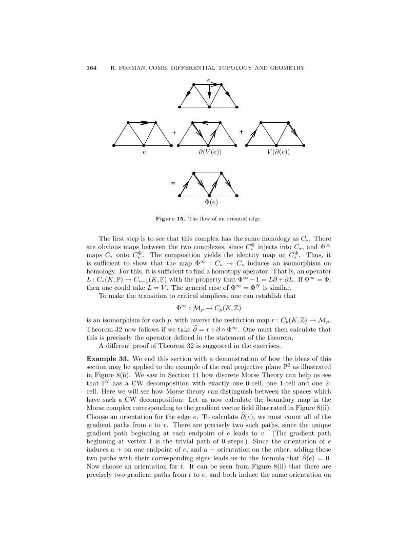
Figure 15. The flow of an oriented edge.
The first step is to see that this complex has the same homology as C∗. Thereare obvious maps between the two complexes, since CΦ∗ injects into C∗, and Φ∞
maps C∗ onto CΦ∗ . The composition yields the identity map on CΦ
∗ . Thus, itis sufficient to show that the map Φ∞ : C∗ → C∗ induces an isomorphism onhomology. For this, it is sufficient to find a homotopy operator. That is, an operatorL : C∗(K, F) → C∗−1(K, F) with the property that Φ∞ − 1 = L∂ + ∂L. If Φ∞ = Φ,then one could take L = V . The general case of Φ∞ = ΦN is similar.
To make the transition to critical simplices, one can establish that
Φ∞ : Mp → Cp(K, Z)
is an isomorphism for each p, with inverse the restriction map r : Cp(K, Z) → Mp.Theorem 32 now follows if we take ∂ = r ◦ ∂ ◦ Φ∞. One must then calculate thatthis is precisely the operator defined in the statement of the theorem.
A different proof of Theorem 32 is suggested in the exercises.
Example 33. We end this section with a demonstration of how the ideas of thissection may be applied to the example of the real projective plane P2 as illustratedin Figure 8(ii). We saw in Section 11 how discrete Morse Theory can help us seethat P2 has a CW decomposition with exactly one 0-cell, one 1-cell and one 2-cell. Here we will see how Morse theory can distinguish between the spaces whichhave such a CW decomposition. Let us now calculate the boundary map in theMorse complex corresponding to the gradient vector field illustrated in Figure 8(ii).Choose an orientation for the edge e. To calculate ∂(e), we must count all of thegradient paths from e to v. There are precisely two such paths, since the uniquegradient path beginning at each endpoint of e leads to v. (The gradient pathbeginning at vertex 1 is the trivial path of 0 steps.) Since the orientation of einduces a + on one endpoint of e, and a − orientation on the other, adding thesetwo paths with their corresponding signs leads us to the formula that ∂(e) = 0.Now choose an orientation for t. It can be seen from Figure 8(ii) that there areprecisely two gradient paths from t to e, and both induce the same orientation on

LECTURE 2. DISCRETE MORSE THEORY, CONTINUED 165
e, so that ∂(t) = ±2e. By reversing the chosen orientation on t if necessary, wemay assume that ∂(t) = 2e. Therefore the homology of the real projective planecan be calculated from the following differential complex.
Z×2−−−−→ Z
0−−−−→ Z −−−−→ 0.
Thus we see that
H0(P2, Z) ∼= Z, H1(P2, Z) ∼= Z/2Z, H2(P2, Z) ∼= 0.
4. Canceling Critical Points
One of the main problems in Morse theory, whether in the combinatorial or smoothsetting, is to find a Morse function, or equivalently a gradient vector field, for agiven space with the fewest possible critical points (much of the book [80] is devotedto this topic). In general this is a very difficult problem, since, in particular, itcontains the Poincare conjecture – spheres can be recognized as those spaces whichhave a Morse function with precisely 2 critical points. In [72], Milnor presentsSmale’s proof [83] of the higher dimensional Poincare conjecture (in fact, a proof ispresented of the more general h-cobordism theorem) completely in the language ofMorse theory. Drastically oversimplifying matters, the proof of the higher Poincareconjecture can be described as follows. Let M be a smooth manifold of dimension≥ 5 which is homotopy equivalent to a sphere. Endow M with a (smooth) Morsefunction f . One then proceeds to show that the critical points of f can be canceledout in pairs until one is left with a Morse function with exactly two critical points,which implies that M is a (topological) sphere.
A key step in this proof is the “cancellation theorem” which provides a sufficientcondition for two critical points to be canceled (see Theorem 5.4 in [72], whichMilnor calls “The First Cancellation Theorem”, or the original proof in [74]). In thissection we will see that the analogous theorem holds for discrete Morse functions.Moreover, in the combinatorial setting the proof is much simpler. The main resultis that if α(p) and β(p+1) are 2 critical simplices, and if there is exactly 1 gradientpath from β to α, then α and β can be canceled. More precisely,
Theorem 34. Suppose V is a discrete gradient vector field on M such that β(p+1)
and α(p) are critical, and there is exactly one V -path from β to α. Then there isanother gradient vector field W on M with the same critical simplices except thatα and β are no longer critical. Moreover, W is equal to V except along the uniquegradient path from β to α.
In the smooth case, the proof, either as presented originally by Morse in [74]or as presented in [72], is rather technical. In our discrete case the proof is simple.If, in the top drawing in Figure 16, the indicated gradient path is the only V -pathfrom β to α, then we can reverse the gradient vector field along this path, replacingV by the vector field W shown in the bottom drawing in Figure 14.
The uniqueness of the V -path implies that the resulting discrete vector fieldhas no closed orbits, and hence, by Theorem 2, is a gradient vector field. Moreover,α and β are not critical for this new gradient vector field, while the criticality ofall other simplices is unchanged. This completes the proof.
The proof in the smooth case proceeds along the same lines. However, inaddition to turning around those vectors along the unique gradient path from βto α, one must also adjust all nearby vectors so that the resulting vector field is

166 R. FORMAN, COMB. DIFFERENTIAL TOPOLOGY AND GEOMETRY
αβ
Figure 16. Canceling critical simplices.
smooth. Moreover, one must check that the new vector field is a gradient vectorfield, so that, in particular, modifying the vectors did not result in the creation ofa closed orbit. This is an example of the sort of complications which arise in thesmooth setting, but which do not make an appearance in the discrete theory.
This theorem was recently put to very good use in [7], in which discrete Morsetheory is used to determine the homotopy type of some simplicial complexes arisingin the study of partitions. It is fascinating, and quite pleasing, to see the sameidea play a central role in two subjects, the Poincare conjecture and the study ofpartitions, which seem to have so little to do with one another. In [50], Hershgeneralizes this cancellation technique and investigates, among other ideas, whenfamilies of pairs of critical simplices can be canceled simultaneously. The maintheorem of this section is also used extensively in [54] as a basic computationaltool for searching for optimal gradient vector fields. To see other computationalapproaches to finding optimal gradient vector fields, the reader can take a look at[62], [63], [64].
5. Exercises for Lecture 2
(1) In the lecture we found a perfect gradient vector field on the complex Δn
of disconnected graphs on n vertices. Since our construction began bycollapsing everything towards the graph g containing only the edge [1, 2]we saw that this is equivalent to the construction of a perfect gradientvector field on the complex of connected graphs on n vertices. The criticalconnected graphs are precisely the critical disconnected graphs with theedge [1, 2] added. The result is the set of increasing trees on n-vertices.That is, the trees with vertex set {1, 2, . . . , n} with the property that thelabels increase along every ray starting at vertex 1. Note that there are(n−1)! of these, and each contains (n−1) edges (and thus corresponds toa simplex of dimension (n − 2)). Consider the collection Pn of graphs onn-vertices which are paths with one endpoint labeled 1. That is, graphsof the form
1 − v2 − v3 − · · · − vn
where {v2, v3, . . . , vn} = {2, 3, . . . , n}. We observe that there are precisely(n−1)! of these graphs, and each has (n−1) edges. Your job is to constructa gradient vector field on the simplicial complex of connected graphs on

LECTURE 2. DISCRETE MORSE THEORY, CONTINUED 167
n vertices for which the critical graphs are precisely the graphs in Pn.(In Vassiliev’s original work on this complex, this is the form in which hepresented the answer.)
(2) Let G be any graph, and let P be any monotone decreasing graph property.Then we can consider the simplicial complex of all spanning subgraphs ofG that satisfy P.
In the lecture we only considered the case where G is a completegraph. For other graphs G, these complexes are quite interesting andlargely unexplored.(a) Examine this in the case where P is the property of being discon-
nected. What is the homotopy type of the resulting complex? Thatis, given a graph G, what is the homotopy type of the simplicialcomplex of disconnected spanning subgraphs of G?
(b) Pick your favorite monotone graph property and your favorite graphand examine the resulting simplicial complex.
(3) Let M be a simplicial complex with a gradient vector field V. Prove thatthe homology of the Morse complex (as defined in this lecture) is isomor-phic to the homology of M by following these steps:(a) Suppose that V is the empty gradient vector field. Then the Morse
complex is just the standard simplicial chain complex of M.(b) Now prove that the homology of the Morse complex of V does not
change if one pair is removed from V (i.e. if one arrow is erased). Dothis by showing that if
M : 0 → Mnd→ Mn−1
d→ Mn−2d→ · · · d→ M0 → 0
and
M ′ : 0 → M ′n
d′→ M ′n−1
d′→ M ′n−2
d′→ c . . .d′→ M ′
0 → 0
are the Morse complexes corresponding to gradient vector fields Vand V ′ on M which differ by a single arrow, then there is a mapΦ : Mi → M ′
i which induces an isomorphism on homology. Try toconstruct the map Φ as explicitly as possible.
Together (a) and (b) prove the desired result.(4) In the exercises to Lecture 1 we proved that every triangulated surface has
a perfect gradient vector field. Consider the Morse complex correspondingto such a vector field. Prove that all of the differentials vanish (that is,each differential is the zero map). Can you understand this directly fromthe definition of the differential – that is by counting gradient paths?

LECTURE 3Discrete Morse Theory and Evasiveness
1. The Main Results
So far, we have indicated some applications of discrete Morse theory to combi-natorics and topology. We now present an application to computer science. Thereader should see the reference [36] for a more complete treatment of the contentof this section.
There is a wide variety of situations in which one has the ability to quickly ask aseries of yes/no questions, with the goal of answering a more difficult question. Forexample, when one goes to the doctor with an illness, the doctor usually asks a seriesof yes/no questions, such as “Do you have a headache?”, “Do you have a fever?”,etc., using the information from the previous questions to decide what to ask next,with the goal of answering the more difficult question “What illness does my patienthave?”. When one takes a malfunctioning car to the mechanic, the mechanic oftenattempts to analyze the problem by testing the individual components one at atime, using the appropriate tools to ask “Is this component working properly?”,with the goal of answering the more difficult question “What is wrong with thiscar?”. The mathematical study of such questions began with the following sort ofproblem. Suppose that one has a network G of phones, or computers, or... whichwe think of as a collection of nodes, some of which are connected by arcs. Weassume that the nework G is connected. That is, one can get from any node to anyother node by a series of arcs. Now we suppose that there is an electrical storm,or a terrorist attack, or..., and some of the arcs are disabled. At that time, ourfirst concern may not be “What is the precise network that remains?” but rather,we may primarily concerned with questions such as “Is the remaining network stillconnected?”. This is the difficult question we wish to answer. We suppose furtherthat we have the capability of testing each arc in the original network, in orderto answer the question “Is this arc still working?”. Of course, we can answer anyquestion about the network if we simply test every arc in the original network,and determine precisely which of these arcs are still working, as that completelydetermines the remaining network. The precise question we want to analyse hereis “Can one do any better?”. That is, is there any strategy for testing the arcssuch that we are guaranteed that we can answer the desired question before havingtested each of the original arcs.
169

170 R. FORMAN, COMB. DIFFERENTIAL TOPOLOGY AND GEOMETRY
yes
no yes
c
a
aab b
b
[ ] [b] [a] [a,b] [c] [a,c] [b,c] [a,b,c]
no
no no
yes no yes no yes no yes
yes
σ =
Figure 17. A search algorithm.
Let us begin with a simple example of the sort of thing we wish to study.Suppose there are three yes/no questions that we can easily ask. We label thesequestions {a, b, c}.Assumption 1: We suppose that these questions have the property that theiranswers are independent of the order in which they are asked. (We will make thisassumption for the rest of these notes.)Then there are eight possible outcomes resulting from asking these three questions.We label these outcomes by listing the questions that yield the answer “yes” forthat outcome. The possibilities are: [ ], [a], [b], [c], [ab], [ac], [bc], [abc].Assumption 2: We assume that every set of answers is possible.That is, one can easily imagine a set of questions with the property that questionsb and c can not both be answered “yes”, but we will not consider this possibilityin these lectures. We make this assumption only for reasons of simplicity. Thegeneral situation is considered in [41]. Suppose that the following four outcomesare good: [a],[b],[c],[ab], and the remaining outcomes are bad. By asking these threequestions, our goal is to determine whether the outcome is good or bad. We can,of course, accomplish this goal by asking all three questions. We are consideredto have won this game if we achieve the goal before we ask the third question. Awinning strategy, then, is one which guarantees that no matter what the outcome is,we can determine whether or not it is good or bad before asking the third question.
For example, consider the search algorithm shown in Figure 17, in which casewe have listed the question to be asked next, given the answers to the previousquestions. For example, we ask question c first, and if we get the answer “yes” weask question b, but if we get the answer “no”, we ask the question a. We observe that,asking questions in the indicated order, if the outcome is in the set {[ ], [b], [c], [ac]},then we must ask the third question. Outcomes which require us to ask the thirdquestion are called evaders of the search algorithm, so the algorithm has 4 evaders.In fact, this is the best one can do. The following proposition is fairly easy to checkby straightforward means.
Proposition 35. Every search algorithm for the problem of determining member-ship in the set of good outcomes {[a], [b], [c], [ab]} has at least 4 evaders. The numberof evaders which are good equals the number of evaders which are bad, and hencethere must be at least two of each.
If we assume that each outcome is equally likely, then this proposition impliesthat no matter which search algorithm we choose, we will have to ask the thirdquestion at least half of the time. Note that this theorem does not say that everysearch algorithm has exactly 4 evaders, and it is rather easy to find search algorithms

LECTURE 3. DISCRETE MORSE THEORY AND EVASIVENESS 171
a
b c
ab
bc
acabc
Figure 18. A topological approach to the problem.
with more than 4 evaders. If every search algorithm has some evaders, so that wehave no winning strategy, then we say that the problem is evasive.
It is probably not at all clear to the reader what this topic is doing in a seriesof lectures on discrete Morse theory, but we will show that in fact these topics areintimately related. In particular, we will show that algebraic topology gives a wayof understanding why some problems of this form are easy, and others are hard.First we observe that the problem can easily be stated in a more topological way.Consider the 2-dimensional simplex S with vertices labeled {a, b, c}. Then the facesof S can be indentified with the subsets of {a, b, c}, and hence with the 8 possibleoutcomes (see Figure 18). Then the good and bad outcomes partition the faces ofS into 2 sets. In this setting we are given a partition of the set of faces, the outcomeis a face σ of the simplex, and our goal is to determine which block of the partitioncontains σ. We are permitted to ask questions of the form “Is vertex v in σ?”.
In this way, we can convert binary search problems (which satisfy Assumption1) into the language of simplices. If we also require Assumption 2, then the sortof search problems we are considering lead to problems of the following form. LetS be an n-dimensional simplex, with vertices v0, v1, . . . , vn, F the set of faces of S,and
P : F = P1 � P2 � . . . � Pk
a partition of F, which is known to you. Let σ be a face of S which is not knownto you. Your goal is to determine which block of the partition P contains σ. Inparticular, you need not determine the face σ. You are permitted to ask questionsof the form “Is vi in σ?”. You may use the answers to the questions you havealready asked in determining which vertex to ask about next. Of course, you candetermine which block contains σ by asking n + 1 questions, since by asking aboutall n+1 vertices you can completely determine σ. You win this game if you answerthe given question after asking fewer than n + 1 questions.
Say that P is nonevasive if there is a winning strategy for this game, i.e thereis a search algorithm that determines which block contains σ in fewer than n + 1questions, no matter what σ is. Say P is evasive otherwise.
One of the main issues we will have to deal with is that a block Pi of thepartition need not be a subcomplex or have any other nice structure. Hence, thenotion of the homology of such a set is problematic. Let P be any set of facesof a simplex S, and let F be a field. One of the main contributions of this andthe following sections is a definition of the F-Betti numbers of P. More precisely,for each i = −1, 0, 1, . . . , we will define Bi(P, F), the ith Betti number of P withrespect to the field F. We will also define the even and odd Betti numbers, denotedBe(P, F) and Bo(P, F), respectively, and the total Betti number B(P, F). For ease ofnotation, we will assume that the field F is fixed, and refer to Bi(P ), Be(P ), Bo(P )

172 R. FORMAN, COMB. DIFFERENTIAL TOPOLOGY AND GEOMETRY
and B(P ). We will present the precise definition of these numbers in the nextsection. The basic idea is that the Betti number Bi(P ) is defined by restrictingthe chain complex of S over the field F to the faces in P . The result need not bea complex, since the composition of its consecutive differentials might be nonzero,but the dimension of its ith “homology” can still be defined as the dimension of itsith kernel minus the dimension of its (i + 1)st image (if that is nonnegative, and 0otherwise); see Proposition 47. At this point, we will state the main properties ofthese Betti numbers.
Theorem 36. For any set of faces P
(i) Be(P ) ≥∑
i even
Bi(P ),
Bo(P ) ≥∑i odd
Bi(P ),
B(P ) = Be(P ) + Bo(P ).
(ii) Bi(P ) = 0 for i larger than the dimension of P .(iii) Be(P ) − Bo(P ) = χ(P ) =
∑i(−1)i#{i-simplices in P}
Our notion of a Betti number is equal to a standard notion in a number of settings.
Theorem 37.(1) If P is a subcomplex of S, and the empty set (considered as a face of S)
is an element of P , then for each i
Bi(P ) = dim Hi(P, F).
where the tilde denotes reduced homology. Moreover,
Be(P ) = dim Heven(P, F)
Bo(P ) = dim Hodd(P, F)
B(P ) = dim H∗(P, F).(2) If P is a subcomplex of S, except that the empty set is not element of P ,
then for each iBi(P ) = dim Hi(P, F).
Moreover,Be(P ) = dimHeven(P, F)Bo(P ) = dim Hodd(P, F)B(P ) = dim H∗(P, F).
(3) Let P denote the closure of P (i.e. the set consisting of the faces of P
along with all of their faces), and let P = P − P. If P is a subcomplex ofS (which contains the empty set) then for each i
Bi(P ) = dimHi(P , P, F).
MoreoverBe(P ) = dimHeven(P , P, F)Bo(P ) = dimHodd(P , P, F)B(P ) = dimH∗(P , P, F).
Assuming these results for now, as well as the still undefined notion of Bettinumber, we present the main theorem of this section.

LECTURE 3. DISCRETE MORSE THEORY AND EVASIVENESS 173
Theorem 38. With all notation as above, for any search algorithm A the numberof evaders of A which lie in any block Pj of the partition P is at least B(Pj). Hencethe total number of evaders is at least
∑kj=1 B(Pj).
In fact, we can make this statement much more precise. Define the dimensionof an evader to be the dimension of the face of S to which it corresponds. That is,if σ is any possible outcome, dim(σ) is
(the number of questions answered “yes” if the outcome is σ) − 1.
Theorem 39. With all notation as above, for any search algorithm A the numberof evaders of A of dimension i which lie in any block Pj of the partition P is atleast Bi(Pj). The number of even-dimensional evaders which lie in block Pj is atleast Be(Pj), and the number of odd-dimensional evaders which lie in block Pj is atleast Bo(Pj) .
Before discussing the proof of this result, we would like to point out that Kahn,Saks and Sturtevant [55] first observed the relationship between evasiveness andalgebraic topology. In their setting, the partition consists of precisely two blocks,P : S = P1 �P2, in which P1 is a subcomplex. They proved the following theorem.
Theorem 40. If H∗(P1) �= 0, where H∗(P1) denotes the reduced homology of P1,then P is evasive.
In fact, they proved something stronger, and we will come back to this pointlater. In [39] we used discrete Morse theory to make some of their results morequantitative along the lines of Theorems 38 and 39. The generalization in thissection to more than two blocks is relatively minor. The extension to more generalsets of faces is the major value of this newer work.
We illustrate the previous theorems by returning to the example introducedat the beginning of this section. Let P1 denote the set {[a], [b], [c], [ab]} of goodoutcomes, and let P2 denote the complement, the set of bad outcomes. We observethat P1 is a simplicial complex which does not contain the empty face. Hence byTheorem 37, B(P1) is equal to the dimension of the (unreduced) homology of P1,which is 2. By Theorem 38, we learn that for any search algorithm, the number ofevaders which lie in P1 is at least 2. We observe that P2 does not satisfy any ofthe hypotheses presented in Theorem 37, so one can not deduce its Betti numbersfrom that result. However, as the reader can check (after we present the definitionof Betti numbers in the next section), its total Betti number is also 2.
The link between evasiveness and algebraic topology is provided by discreteMorse theory. Morse theory comes to the fore when one observes that a searchalgorithm induces a discrete vector field on S. For example, the search algorithmshown in Figure 17 induces the vector field
V = { {[ ] < [b]}, {[a] < [a, b]}, {[c] < [a, c]}, {[b, c] < [a, b, c]} }That is, V consists of those pairs of faces of S which are not distinguished by thesearch algorithm until the last question. There is slight subtlety here in that a searchalgorithm pairs a vertex with the empty face [ ], while in our original definition, itwas not permitted to pair a simplex with [ ]. Thus, to get a true discrete vectorfield, we must remove this pair from V . (It is precisely this subtle point that resultsin the reduced homology of K being the relevant measure of topological complexity

174 R. FORMAN, COMB. DIFFERENTIAL TOPOLOGY AND GEOMETRY
a
b c
ab
bc
acabc
Figure 19. The induced vector field V .
in Theorem 37(1), rather than the unreduced homology.) However, for simplicity,from now on we will simply ignore this technical point.
Theorem 41. For any search algorithm, let V denote the vector field consisting ofpairs of nonempty faces of S which are not distinguished by the search algorithmuntil the last question. Then V is a gradient vector field.
We will postpone the proof of this result until the end of this section.For now, suppose that block Pj of the partition P is a subcomplex (containing
the empty face). We will complete the proof in this setting before discussing thegeneral case. Now restrict V to Pj by taking only those pairs in V such that bothsimplices are in Pj , and denote the resulting vector field by Vj . In our simpleexample, this results in the vector field
V1 = {{[a] < [a, b]}}.From the previous theorem, V has no closed orbits. Any discrete vector fieldconsisting of a subset of the pairs of V has fewer paths, and hence also has noclosed orbits. Therefore, Vj is a gradient vector field on Pj . Note that V pairsevery face of S with another face, and hence there are no critical simplices exceptfor the vertex which is paired with the empty set. Thus, ignoring that special vertexfor the moment, the critical simplices of Vj are precisely the simplices of Pj whichare paired in V with a face of S which is not in Pj . These are precisely the simplicesof Pj which are the evaders of the search algorithm.
The Morse inequalities of Theorem 13 (i) immediately imply the following re-sult.
Corollary 42. If the block Pj of the partition P is a subcomplex (containing theempty face of S) then the number of evaders in Pj is at least dim H∗(Pj).
(We must use reduced homology here because of the minor issue surrounding thevertex paired with the empty set.) This yields Theorem 37 (in the case of a sim-plicial complex containing the empty face).
Suppose that P is nonevasive. Then there is some search algorithm which hasno evaders. From our above discussion we have seen that this implies that Pj has agradient vector field with no critical simplices. Actually, this is not quite true. Thegradient vector field must have a critical vertex – the vertex that is paired with theempty face. These ideas lead to the following strengthening of Theorem 40.
Theorem 43. If P is nonevasive, and if the block Pj of the partition is a subcom-plex, then Pj collapses to a vertex.
This theorem appears in [55], the paper that first established, and used to verygood effect, a close relationship between evasiveness and topology. The interested

LECTURE 3. DISCRETE MORSE THEORY AND EVASIVENESS 175
reader can consult [36] for some additional refinements of this theorem. This topichas been the subject of much study, and the reader can find more information aboutthe connection between evasiveness and topology in the references [11], [56], [76],[77], and [94] .
We now present a proof of Theorem 41. Let S denote an n-simplex, and fix asearch algorithm. Associate to each p-simplex α of S the sequence of integers
n(α) = n0(α) < n1(α) < · · · < np(α)
where, for each i, question number ni(α) is answered “yes” if σ = α, and these arethe only questions answered “yes”.
Let V be the vector field induced by the search algorithm and
α1, α2
be a V -path. Then either (i) α1 is a face of α2 and {α1 < α2} ∈ V, or (ii) α2 is aface of α1 and {α1 < α2} /∈ V. Let us consider case (ii) first. In this case, α2 hasone fewer vertex than α1, and the vertex is not the subject of the (n+1)st question.Suppose the the vertex is the subject of the ni(α1)st question. Then this questionis answered “yes” for α1, but “no” for α2. This implies that
n(α2) = n0(α1) < n1(α1) < · · · < ni−1(α1) < ni(α2) < · · ·for some i < n + 1, and such that ni(α2) > ni(α1). Thus n(α2) > n(α1) in thelexicographic order.
We now consider case (i), in which {α1 < α2} ∈ V, and continue the V -path onemore step to α1, α2, α3. Then α1 and α2 are not distinguished until the (n + 1)st
question. Thus,
n(α2) = n0(α1) < n1(α1) < · · · < np(α1) < n + 1.
We now observe that the vertices of α3 are a subset of the vertices of α2. Supposethe vertex of α2 which is not in α3 is the vertex tested in question ni(α2). Thenwe must have i �= n + 1. This demonstrates that
n(α3) = n0(α1) < n1(α1) < · · · < ni−1(α1) < ni(α3) < · · ·for some i < n + 1, and such that ni(α3) > ni(α1). Thus n(α3) > n(α1) in thelexicographic order, which is sufficient to prove that there are no closed orbits.
In [53], Jonsson investigates further the question of which gradient vector fieldsarise from decision trees. Anyone interested in this topic should also consult [84].
2. Betti Numbers for General Sets of Faces
In this section we examine how to extend the results of the previous section to setsof faces of a simplex that do not form a simplicial complex or have any other specialstructure. A more extensive treatment of these ideas can be found in [41]. Let Fbe any field. Let
V : 0 −−−−→ Vn∂n−−−−→ Vn−1
∂n−1−−−−→ · · · ∂1−−−−→ V0∂0−−−−→ V−1 −−−−→ 0
be a complex of finite dimensional vector spaces over the field F. The ∂i’s areassumed to be linear maps, but we are not assuming that ∂d ◦ ∂d+1 = 0. Our goalis to define the “homology” of this complex.

176 R. FORMAN, COMB. DIFFERENTIAL TOPOLOGY AND GEOMETRY
If ∂p ◦∂p+1 = 0 for each p, then we say that V is a differential complex and thatthe ∂i’s form a differential. We recall that one defines the homology of a differentialcomplex by the formula
(5) Hp(V) :=Ker ∂p
Im ∂p+1.
For each p, choose a subspace Xp which is mapped isomorphically onto Im ∂p. Thenwe have that
Vp = Xp ⊕ Ker ∂p.
In the case of a differential complex, Im ∂p+1 ⊂Ker ∂p we can find a Zp ⊂ Vp sothat
Ker ∂p = Im ∂p+1 ⊕ Zp,
which implies thatVp = Xp ⊕ Im ∂p+1 ⊕ Zp,
and the reader can easily check that Zp∼= Hp(V).
We now return to the general case of a nondifferential complex. That is, weno longer assume that ∂p ◦ ∂p+1 = 0. We will use the construction of the previousparagraph to define the homology of such a complex.
Definition 44. A homological decomposition D of the complex S is a decomposi-tion
Vi = Xi ⊕ Yi ⊕ Zi,
for each i, with the property that for each i, ∂i maps Xi isomorphically onto Yi−1.
By the notation Vi = Xi ⊕Yi ⊕Zi we mean that Xi, Yi and Zi are linear subspacesof Vi, such that their pairwise intersections are {0}, and they sum to give all of Vi.Homological decompositions always exist, since one can take Xi = 0, Yi = 0, andZi = Vi, for each i.
For any homological decomposition D of V , and any i, let Bi(V , D) denote thedimension of Zi. We also define the even Betti number of D
Be(V ,D) :=∑
i even
Bi(V ,D),
the odd Betti number of D
Bo(V ,D) =∑i odd
Bi(V ,D),
and the total Betti number of D
B(V ,D) = Be(V ,D) + Bo(V ,D) =∑
i
Bi(V ,D).
We now define the Betti numbers of S by
Bi(V) := minD
Bi(V ,D),
Be(V) := minD
Be(V ,D),
Bo(V) := minD
Bo(V ,D),
andB(V) := min
DB(V ,D).
We observe the following facts.
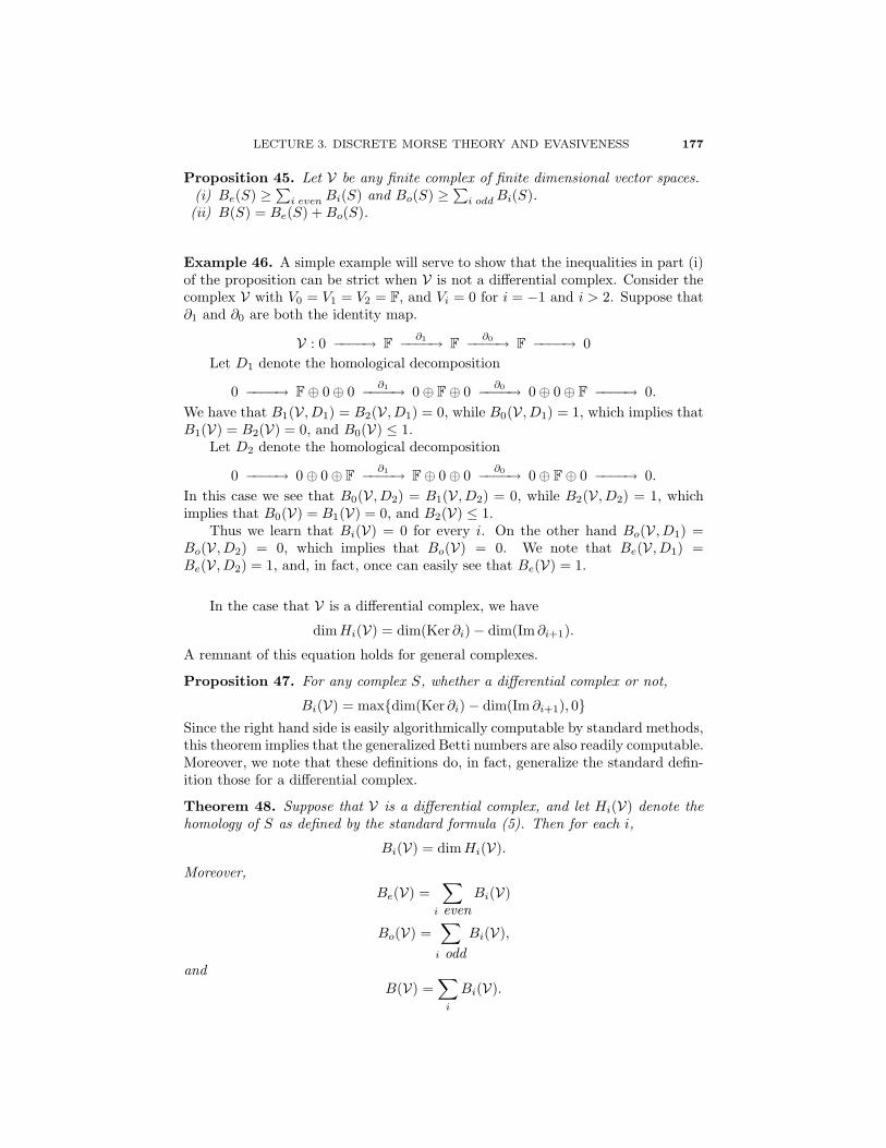
LECTURE 3. DISCRETE MORSE THEORY AND EVASIVENESS 177
Proposition 45. Let V be any finite complex of finite dimensional vector spaces.(i) Be(S) ≥∑i even Bi(S) and Bo(S) ≥∑i odd Bi(S).(ii) B(S) = Be(S) + Bo(S).
Example 46. A simple example will serve to show that the inequalities in part (i)of the proposition can be strict when V is not a differential complex. Consider thecomplex V with V0 = V1 = V2 = F, and Vi = 0 for i = −1 and i > 2. Suppose that∂1 and ∂0 are both the identity map.
V : 0 −−−−→ F∂1−−−−→ F
∂0−−−−→ F −−−−→ 0Let D1 denote the homological decomposition
0 −−−−→ F ⊕ 0 ⊕ 0 ∂1−−−−→ 0 ⊕ F ⊕ 0 ∂0−−−−→ 0 ⊕ 0 ⊕ F −−−−→ 0.
We have that B1(V , D1) = B2(V , D1) = 0, while B0(V , D1) = 1, which implies thatB1(V) = B2(V) = 0, and B0(V) ≤ 1.
Let D2 denote the homological decomposition
0 −−−−→ 0 ⊕ 0 ⊕ F∂1−−−−→ F ⊕ 0 ⊕ 0 ∂0−−−−→ 0 ⊕ F ⊕ 0 −−−−→ 0.
In this case we see that B0(V , D2) = B1(V , D2) = 0, while B2(V , D2) = 1, whichimplies that B0(V) = B1(V) = 0, and B2(V) ≤ 1.
Thus we learn that Bi(V) = 0 for every i. On the other hand Bo(V , D1) =Bo(V , D2) = 0, which implies that Bo(V) = 0. We note that Be(V , D1) =Be(V , D2) = 1, and, in fact, once can easily see that Be(V) = 1.
In the case that V is a differential complex, we have
dimHi(V) = dim(Ker ∂i) − dim(Im ∂i+1).
A remnant of this equation holds for general complexes.
Proposition 47. For any complex S, whether a differential complex or not,
Bi(V) = max{dim(Ker ∂i) − dim(Im ∂i+1), 0}Since the right hand side is easily algorithmically computable by standard methods,this theorem implies that the generalized Betti numbers are also readily computable.Moreover, we note that these definitions do, in fact, generalize the standard defin-ition those for a differential complex.
Theorem 48. Suppose that V is a differential complex, and let Hi(V) denote thehomology of S as defined by the standard formula (5). Then for each i,
Bi(V) = dimHi(V).
Moreover,Be(V) =
∑i even
Bi(V)
Bo(V) =∑
i oddBi(V),
andB(V) =
∑i
Bi(V).

178 R. FORMAN, COMB. DIFFERENTIAL TOPOLOGY AND GEOMETRY
Now let S be a simplex. A simplex space is defined to be a set of faces of S(we consider the empty set to be a face of S). Let K be a simplex space. Fix afield F and let Cd(K, F) denote the oriented d-chains in K. This is defined in theusual way, even if K is not a subcomplex, that is, for all d ≥ 2, let Sd(K) denotethe set of pairs (σ, ε), where σ is a d-simplex in K, and ε is an orientation on σ(i.e. an ordering of the vertices in σ modulo even permutations – so that each σ hastwo distinct orientations). We let Cd(K, F) denote the vector space of all formallinear combinations of elements in Sd(K), and Cd(K, F) the result of quotientingout Cd(K, F) by the relation −1(σ, ε) = (σ,−ε), where if ε denotes an orientation ona d-simplex σ, then −ε denotes the alternate orientation. If d = −1, 0, then each d-simplex in K has a unique orientation, and we let Cd(K, F) denote the vector spaceof all formal linear combinations of d-simplices. Note that the only possible −1-dimensional simplex is the empty simplex. Thus, if K contains the empty simplexC−1(K, F) ∼= F and otherwise C−1(K, F) ∼= 0.
We now define a boundary map ∂d from Cd(K, F) to Cd−1(K, F), by setting,for any oriented d-simplex [x0, x1, . . . , xd],
∂d[x0, x1, . . . , xd] =∑
i
′(−1)i[x0, x1, . . . , xi−1, xi+1, . . . , xd].
where the notation∑′ means that the sum is over all i ⊂ {0, 1, 2, . . . , d} such
that the simplex {x0, x1, . . . , xi−1, xi+1, . . . , xd} is in K. As usual, the notation[x0, x1, . . . , xd] denotes the simplex {x0, x1, . . . , xd} along with the orientation in-duced by ordering the vertices in the manner in which they are listed.
We let C(K, F) denote the complex
0 −−−−→ Cn(K, F) ∂n−−−−→ . . .∂0−−−−→ C−1(K, F) −−−−→ 0.
Using the notation of the previous section, we denote by
Bi(K, F), Be(K, F), Bo(K, F), B(K, F),
the numbers
Bi(C(K, F)), Be(C(K, F)), Bo(C(K, F)), B(C(K, F)).
We observe that if K is a simplicial complex, and contains the empty simplex,then C(K, F) is the usual reduced chain complex. If K is a simplicial complex exceptthat K does not contain the empty simplex, then C(K, F) is the usual (nonreduced)chain complex. If K = K − K is a nonempty subcomplex (where K denotes theclosure of K, i.e. K along with all of the faces of the elements in K, and K denotesthe elements in K which are not in K), then C(K, F) is isomorphic to the relativechain complex C(K, K, F). In particular, in these cases, C(K, F) is a differentialcomplex, so, by Theorem 48, the Betti numbers we have defined are equal to thestandard Betti numbers. This implies Theorem 37.
Example 49. Let S denote the two-dimensional simplex with vertices labeled a,b, c. Let K denote the simplex space consisting of the faces [c], [b, c] and [a, b, c](Figure 20). The chain complex for K can easily seen to be isomorphic to thecomplex examined in Example 46. From the calculations done there, we see thatBi(K) = 0 for each i = −1, 0, 2, . . . , and Bo(K) = 0, while B(K) = Be(K) = 1.
The next goal is to indicate that these Betti numbers allow us to apply the basicnotions of discrete Morse theory to general simplex spaces. Let K be a simplex
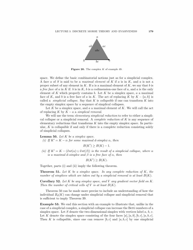
LECTURE 3. DISCRETE MORSE THEORY AND EVASIVENESS 179
a
b c
ab
bc
ac
abc
Figure 20. The complex K of example 49.
space. We define the basic combinatorial notions just as for a simplicial complex.A face a of S is said to be a maximal element of K if a is in K, and a is not aproper subset of any element in K. If a is a maximal element of K, we say that b isa free face of a in K if: b is in K, b is a codimension-one face of a, and a is the onlyelement of K which properly contains b. Let K be a simplex space, a a maximalface of K, and b is a free face of a in K. The act of replacing K by K − {a, b} iscalled a simplicial collapse. Say that K is collapsible if one can transform K intothe empty simplex space by a sequence of simplical collapses.
Let K be a simplex space, and a a maximal element of K. We will call the actof replacing K by K − a a simplical removal.
We will use the term elementary simplicial reduction to refer to either a simpli-cal collapse or a simplicial removal. A complete reduction of K is any sequence ofelementary reductions that transforms K into the empty simplex space. In partic-ular, K is collapsible if and only if there is a complete reduction consisting solelyof simplicial collapses.
Lemma 50. Let K be a simplex space.(i) If K ′ = K − α for some maximal d-simplex α, then
B(K ′) ≥ B(K) − 1.
(ii) If K ′ = K − (Int(α) ∪ Int(β)) is the result of a simplicial collapse, where αis a maximal d-simplex and β is a free face of α, then
B(K ′) ≥ B(K).
Together, parts (i) and (ii) imply the following theorem.
Theorem 51. Let K be a simplex space. In any complete reduction of K, thenumber of simplices which are taken out by a simplicial removal is at least B(K).
Corollary 52. Let K be any simplex space, and V any gradient vector field on K.Then the number of critical cells of V is at least B(K).
Theorem 50 can be made more precise to include an understanding of how theindividual Bd(K) can change under simplicial collapse and simplicial removal thatis sufficient to imply Theorem 39.
Example 53. We end this section with an example to illustrate that, unlike in thecase of a simplicial complex, a simplicial collapse can increase the Betti numbers of asimplex space. Let S denote the two-dimensional simplex with vertices label a, b, c.Let K denote the simplex space consisting of the four faces [a], [a, b], [b, c], [a, b, c].Then K is collapsible, since one can remove [b, c] and [a, b, c] by one simplicial
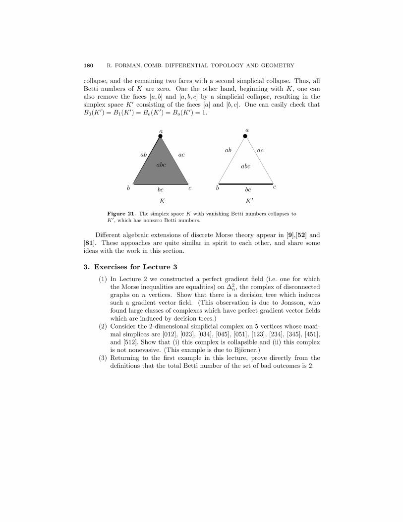
180 R. FORMAN, COMB. DIFFERENTIAL TOPOLOGY AND GEOMETRY
collapse, and the remaining two faces with a second simplicial collapse. Thus, allBetti numbers of K are zero. One the other hand, beginning with K, one canalso remove the faces [a, b] and [a, b, c] by a simplicial collapse, resulting in thesimplex space K ′ consisting of the faces [a] and [b, c]. One can easily check thatB0(K ′) = B1(K ′) = Be(K ′) = Bo(K ′) = 1.
a a
b bc c
abab
bcbc
acac
abc abc
K K ′
Figure 21. The simplex space K with vanishing Betti numbers collapses toK ′, which has nonzero Betti numbers.
Different algebraic extensions of discrete Morse theory appear in [9],[52] and[81]. These appoaches are quite similar in spirit to each other, and share someideas with the work in this section.
3. Exercises for Lecture 3
(1) In Lecture 2 we constructed a perfect gradient field (i.e. one for whichthe Morse inequalities are equalities) on Δ2
n, the complex of disconnectedgraphs on n vertices. Show that there is a decision tree which inducessuch a gradient vector field. (This observation is due to Jonsson, whofound large classes of complexes which have perfect gradient vector fieldswhich are induced by decision trees.)
(2) Consider the 2-dimensional simplicial complex on 5 vertices whose maxi-mal simplices are [012], [023], [034], [045], [051], [123], [234], [345], [451],and [512]. Show that (i) this complex is collapsible and (ii) this complexis not nonevasive. (This example is due to Bjorner.)
(3) Returning to the first example in this lecture, prove directly from thedefinitions that the total Betti number of the set of bad outcomes is 2.

LECTURE 4The Charney-Davis Conjectures
1. Introduction
These notes are intended to be an introduction to the Charney-Davis conjecturesand some of their combinatorial implications. My aim is to provide a stimulatingadvertisement for a circle of ideas that is the subject of some fascinating recentwork, most of which creates more questions than answers, and which has shed newlight on some of the central questions in geometric combinatorics. The subject isa beautiful one, borrowing techniques and ideas from geometry, topology, analysis,algebra, algebraic geometry and combinatorics. My goal in these lectures is topresent the topological and geometric context of these conjectures (as presentede.g. in [15],[22]), along with the most recent combinatorial understanding of them(as in Gal [43] and Branden[12].) These notes will have been successful if somereaders are inspired to consult these original sources, and to begin thinking aboutthese conjectures.
The Charney-Davis conjectures, concerned with the relationship between geom-etry and topology, find their origins, as do most such questions, in the Gauss-BonnetTheorem. Recall that the Gauss-Bonnet theorem states that if M is a compact sur-face with a Riemannian metric, then
χ(M) =12π
∫M
K darea
where K denotes the Gauss curvature of M . It follows that if K ≤ 0 everywhere,then χ(M) ≤ 0.
Hopf conjectured the following generalization.
Conjecture 54. If M is a compact Riemannian manifold of dimension 2n and thesectional curvature of M is ≤ 0 then (−1)nχ(M) ≥ 0.
[Recall that if M is an odd-dimensional manifold, then χ(M) = 0.] This isnot a suitable place for a primer in differential geometry, so we hope it will sufficeto say that the condition that the sectional curvature is nonpositive means thatevery two-dimensional “orthogonal slice” of M is a surface of nonpositive Gausscurvature. This conjecture may seem a bit surprising, and perhaps unintuitive,at first glance. However, some general considerations point in this direction. Mostnotably, one has the following observations.
181

182 R. FORMAN, COMB. DIFFERENTIAL TOPOLOGY AND GEOMETRY
Proposition 55.(1) Let M1 and M2 be compact manifolds, then
χ(M1 × M2) = χ(M1)χ(M2).
(2) If M1 and M2 are Riemannian manifolds with nonpositive sectional cur-vature, and M1 × M2 is endowed with the product Riemannian metric,then M1 × M2 has nonpositive sectional curvature.
Thus, if M1 and M2 are nonpositively curved Riemannian manifolds for whichthe conclusion of Hopf’s conjecture holds, then the same is true for M1×M2. In par-ticular, Hopf’s conjecture holds for any product of arbitrarily many nonpositivelycurved surfaces.
Allendoerfer, Fenchel and Weil ([1],[29], [2]), and later Chern ([17]), proveda higher dimensional version of the Gauss-Bonnet theorem, which, for a compactRiemannian manifold, has the general form
χ(M) =∫
M
R dvol,
where R is a function of the curvature of M and is usually called the Chern-Gauss-Bonnet integrand. Chern [18] gives a proof (attributed to Milnor) that indimension 4, if the sectional curvature is ≤ 0 everywhere, then R ≥ 0. In particular:
Corollary 56. If M is a compact Riemannian 4-manifold with sectional curvature≤ 0, then χ(M) ≥ 0.
However, Geroch [44] proved that this approach is insufficient to settle Hopf’sconjecture in higher dimensions.
Theorem 57. In even dimensions ≥ 6, there exist Riemannian metrics with sec-tional curvature ≤ 0 such that the Chern-Gauss-Bonnet integrand achieves bothsigns.
So, in higher dimensions another approach is necessary. Before discussing al-ternate approaches, and partial results, we will take a detour to discuss some gen-eralizations and extensions of Hopf’s conjecture. From now on, when we say thata Riemannian manifold M has nonpositive curvature, we mean that all sectionalcurvatures are ≤ 0.
It is a theorem of Cartan and Hadamard that if Mn has nonpositive curvature,then M , the universal cover of M , is diffeomorphic to Rn. A manifold is said tobe aspherical if its universal cover is contractible. Thurston generalized Hopf’sconjecture to the following
Conjecture 58. Let M2n be a smooth, compact, aspherical manifold. Then
(−1)nχ(M) ≥ 0.
This is quite interesting, as the hypothesis has changed from a geometric conditionto one that is purely topological. Our interests, however, lie in a different direction.Riemannian curvature is expressed in terms of 2nd derivatives of the metric. Thus,Hopf’s conjecture, as it is usually understood, is a statement about manifolds whichare at least twice differentiable. However, Alexandrov showed how one could speakof nonpositive curvature for continuous, but nonsmooth, manifolds. Let M be acomplete Riemannian manifold. The Hopf-Rinow theorem states that for any twopoints p and q in M , there exists a minimal geodesic from p to q (i.e. a curve γ
LECTURE 4. THE CHARNEY-DAVIS CONJECTURES 183
from p to q satisfying length(γ) = distance(p, q)). Let x, y and z be three pointsin M , and x, y and z be three points in R2 such that
dM (x, y) = dR2(x, y), dM (x, z) = dR2(x, z), and dM (y, z) = dR2(y, z).
(Such x, y and z always exist.) Let γ be a minimal geodesic from y to z, and γ thestraight line from y to z. Since |γ| = |γ| there is a natural identification betweenpoints in γ and points in γ. In [3] Alexandrov proves the following result.
Theorem 59.(1) If M is simply-connected and has nonpositive curvature, then for any point
p in γ, if p is the corresponding point in γ, we have
dM (x, p) ≤ dR2(x, p).
(2) If M is not simply-connected then the above inequality is still true if onerestricts to triples x, y and z which are sufficiently close to one another.
(3) The converse is also true: If the above inequality holds for all sufficientlyclose x, y and z then M has nonpositive curvature.
Alexandrov’s theorem shows that the property of nonpositive curvature is equivalentto a property which can be expressed in terms of the distance function withoutreference to any derivatives. Hence we can use this theorem to make sense of thenotion of nonpositive curvature for spaces without a smooth structure. By replacingR2 with other constant curvature surfaces, we can also make sense of the notion ofhaving curvature bounded above by any real number. While a smooth structureis not necessary, this approach does require the existence of geodesics, so we mustrestrict attention to spaces for which this notion makes sense.
Definition 60. Let M be a metric space.(1) Let x and y be two points in M and d = dist(x, y). Then a (minimal)
geodesic between x and y is an isometry γ : [0, d] → M with γ(0) = x andγ(d) = y.
(2) M is said to be a length space (or a geodesic space) if every pair of pointscan be joined by a geodesic.
Motivated by Alexandrov’s theorem, a length space M is said to be CAT(0) (Cfor Comparison or Cartan, A for Alexandrov, and T for Toponogov, who provedrelated comparison theorems) if the following condition holds: For any three pointsx, y and z in M , let x, y and z be three points in R2 such that
dM (x, y) = dR2(x, y), dM (x, z) = dR2(x, z), and dM (y, z) = dR2(y, z).
Let γ be any minimal geodesic from y to z, and γ′ the straight line from y to z.Let p be any point in γ, and p the corresponding point in γ. Then we require, forall choices of x, y, z, γ and p that
dM (x, p) ≤ dR2(x, p).
Some basic facts about CAT(0) spaces are left as exercises (see the end of thissection).
Parts (2) and (3) of Theorem 59 lead to the following definition (which firstappeared, along with many far-reaching implications and applications of this idea,in [48]).
Definition 61. Say a length space M is nonpositively curved (NP) if the CAT(0)inequality is true for all sufficiently close triples x, p, q.

184 R. FORMAN, COMB. DIFFERENTIAL TOPOLOGY AND GEOMETRY
The basic relationship between these notions is the following.
Theorem 62. M is CAT (0) if and only if M is simply connected and nonpositivelycurved.
We now specialize to a subclass of length spaces, namely polyhedra. A poly-hedron is defined by a set {p1, p2, p3, . . . } of convex polytopes together with acollection of isometric identifications of some faces of the polytopes. Quotientingout by these identifications yields a topological space M which has a given celldecomposition. We require that in the resulting space, if two polytopes meet, theydo so along a face of each. In these notes we also require that there be a uniformupper bound on the diameter of the polytopes, and that the resulting cell complexbe locally finite.
It is useful now to introduce the notion of the link of a vertex. Let M be apolyhedron, and v a vertex of M. For any ε, let S(v, ε) denote the points in M whichlie in a polytope incident to v and whose distance from v is precisely ε. For ε smallenough, S(v, ε) is a topological space with an induced cell decomposition which is,up to isomorphism, independent of ε. This space, along with its cell decomposition,is defined to be the link of v, and is denoted by link(v). If M has the propertythat the link of every vertex is a combinatorial sphere (i.e. it has a subdivisionisomorphic to a subdivision of the boundary complex of a simplex), then M is amanifold. In this case we call M a piecewise Euclidean manifold (or PE manifold).
It will be important later that the link of each vertex comes also with a nat-ural geometry. If ε is the radius of S, we can normalize the metric on S ∩ M bymultiplying by 1/ε, so that the cells of S ∩ M are now convex cells from a sphereof radius 1. When we speak of distances and lengths on link(v), it is always withrespect to this spherical geometry.
For any polyhedron M there is a natural notion of arc-length for curves inM , induced by the Euclidean structure in each polytope. We can then define thedistance between two points in M to be the infimum of the length of the curvesconnecting the two points.
Theorem 63. Any polyhedron with arclength and distance defined as above is alength space.
Thus, using Definition 61, we can speak of a polyhedron having nonpositivecurvature. We can now state the first conjecture of Charney and Davis, which is adirect analogue of Hopf’s conjecture.
Conjecture 64. If M is a nonpositively curved compact PE manifold of dimension2n, then (−1)nχ(M) ≥ 0.
(This conjecture, and all of the other conjectures presented in this section firstappeared in [15], and the reader should certainly consult that paper for a morecomplete discussion, as well as some initial evidence for the conjectures.) Sincethe first positive steps towards the Hopf conjecture were proved using the general-ized Gauss-Bonnet theorem, it seems reasonable to begin our examination of theCharney-Davis conjecture with a similar approach. Let us begin with the case of aPE surface. Let M be a PE surface, and v a vertex of M. Let
(6) k(v) = 1 −∑f>v
angle(f, v),
LECTURE 4. THE CHARNEY-DAVIS CONJECTURES 185
where the sum is over all faces f which contain v, and angle(f, v) ∈ [0, 1] denotesthe normalized interior angle of f at v, i.e. the usual angle (in radians) divided by2π. Then one can check in a straightforward manner the following very classicalformula
(7) χ(M) =∑
v
k(v).
The relationship between the previous discussion and the current topic is providedby the following lemma.
Lemma 65. A PE surface M is nonpositively curved if and only if k(v) ≤ 0 foreach vertex v.
The Charney-Davis conjecture, in the case of PE surfaces, follows immediately.
This discussion was generalized to higher dimensions by Banchoff [8]. Let Mbe a polyhedron and v a vertex of M. Define
(8) k(v) =n∑
i=0
(−1)i∑
{α(i)>v}[v, α]
where {α(i) > v} denotes the set of i-dimensional cells of M which contain v, and[v, α] denotes the normalized exterior angle of α at v. That is, [v, α] is the fractionof the sphere consisting of outward pointing normals to supporting hyperplanes ofα at v. Equivalently, [v, α] is the fraction of linear functions on α which achievetheir maximum at v. Banchoff proved the following generalization of (7).
Theorem 66. If M is a polyhedron, then
(9) χ(M) =∑
v
k(v).
Recall that the local approach that was sufficient to prove Hopf’s theoremin dimensions 2 and 4 is not sufficient in higher directions. Charney and Davis,perhaps somewhat surprisingly, conjecture that the corresponding local approachto their conjecture works in all dimensions.
Conjecture 67. Let M be a PE manifold of dimension 2n. If M is nonpositivelycurved, then for every vertex of M
(−1)nk(v) ≥ 0.
The function k(v) can, in a straightforward way, be written in terms of the linkof v with its natural geometry as a complex of spherical cells. Let k denote thisfunction, so that
k(v) = k(link(v)).The next step is to determine which simplicial complexes can arise as links of
vertices in nonpositively curved PE manifolds. Roughly speaking, a Riemannianmanifold has nonpositive curvature if and only if the boundary of each small metricball is larger, in some sense, than the corresponding Euclidean sphere. Somethingsimilar is true for PE manifolds. That is, a PE manifold is nonpositively curvedif the link is larger, in a precise sense, than a standard sphere of radius 1. Moreprecisely, say that a complex L of spherical cells is large if for every pair of pointsx and y in L, with dist(x, y) < π, there is a unique geodesic connecting them. Thefollowing is a theorem of Gromov [48].
186 R. FORMAN, COMB. DIFFERENTIAL TOPOLOGY AND GEOMETRY
Theorem 68. A PE manifold M is nonpositively curved if and only if the link ofevery vertex is large.
The strongest version (from this point of view) of the Conjecture 67 can nowbe stated.
Conjecture 69. Let L be a spherical complex (i.e. a cell complex in which each cellhas the geometry of a convex cell in a sphere of radius 1) which is homeomorphicto a sphere of dimension 2n− 1. If L is large, then
(−1)nk(L) ≥ 0.
Note that this is a more general conjecture that what is needed, as our originalsetting required consideration only of combinatorial spheres (a more restrictive classthan all topological spheres). However, it does not seem constructive at this pointto quibble over such distinctions, since it is not at all clear what the right contextis for this conjecture. Moreover, in just a moment we will weaken this hypothesiseven further.
For the remainder of these notes, we will restrict attention to the case in whichM is a cubical complex (i.e. all of the polytopal cells in M are geometric cubes).In this case, the links have a very special structure, namely every edge of each ofthe spherical simplices has length π/2. One can easily see that for each α(i) > v,we have [v, α] = (1/2)i. Since each such α corresponds to an (i− 1) simplex in thelink of v, we have the formula
(10) k(L) = 1 +dim(M)−1∑
i=0
(−12)i+1
fi(L),
where fi(L) denotes the number of i-simplices in L. Gromov showed that there isa simple combinatorial test for whether such a link is large.
Definition 70. Say that a simplicial complex L is flag if every clique spans asimplex. That is, is v1, v2, . . . , vk are vertices in L, and they are all pairwiseadjacent, then they span a simplex.
Theorem 71. A cubical PE manifold is nonpositively curved if and only if the linkof every vertex is flag.
Thus, in this case, Conjecture 69 implies the following statement.
Conjecture 72. Let L be a simplicial complex which is homeomorphic to a sphereof dimension 2n − 1. If L is flag, then (−1)nk(L) ≥ 0, where k(L) is given by theformula (10
This conjecture is very combinatorial in nature, but still has one topological,noncombinatorial, ingredient, namely the hypothesis that L be homeomorphic to asphere. There is a natural generalization of triangulated spheres which has a morecombinatorial flavor. A Gorenstein* complex (or a generalized homology sphere)is a simplicial complex with the property that, for every p ≥ 0, the link of everyp-simplex has the homology of an (n − p − 1)-sphere. If L is a simplicial complexwhich is homeomorphic to an n-sphere, or, more generally, any homology n-sphere,then L is Gorenstein*. Thus, to place these ideas in a more combinatorial setting,it is natural to consider the following generalization of Conjecture 72.
LECTURE 4. THE CHARNEY-DAVIS CONJECTURES 187
Conjecture 73. Let L be a (2n − 1)-dimensional Gorenstein* complex. If, inaddition, L is flag, then (−1)nk(L) ≥ 0, where k(L) is given by the formula (10).
It is not at all surprising that this conjecture, which is stated completely incombinatorial terms, has received the most attention from the combinatorics com-munity. We will discuss the connections with other combinatorial notions in Section3. For now we note that this conjecture, or Conjecture 72, implies Conjecture 64 forcubical complexes. It is a simple, but still rather surprising, fact that the converse istrue. The following result is due to Babson-Billera-Chan [5] and Bridson-Haefliger[13].
Theorem 74. Let L be any simplicial complex. Then there is a finite cubicalpolyhedron M with the property that the link of every vertex of M is isomorphic toL.
Proof. Let V denote the vertex set of L. Consider the cube C = [0, 1]V ⊂ RV
endowed with its standard cubical cell decomposition. We will find M as a sub-complex of C. For every simplex σ of L, let Rσ denote the linear subspace of RV
traced out by varying the coordinates corresponding to vertices in σ. Let M bethe union of all faces of C which are parallel to some Rσ, for some simplex σ ofL. Then the vertices of M are the vertices of C, and the link of every vertex isisomorphic to L. �
Applying this result to the case when L is a combinatorial sphere yields acubical PE manifold M. If, in addition, L is flag, it follows from Theorem 71 thatM is nonpositively curved.
Corollary 75. The Charney-Davis Conjecture 64 is true for cubical nonpositivelycurved PE manifolds if and only if Conjecture 72 is true for combinatorial spheres.
2. Exercises for Lecture 4
(1) Prove that if M is a CAT(0) space then(a) For any points p and q ∈ M , there is a unique minimal geodesic from
p to q.(b) M is contractible.
(2) Prove the formula (7) for any triangulated surface M .(3) Prove the formula (9) for any finite polyhedron M .(4) Show that the formula (8) specializes to (6) in the case of a triangulated
surface.(5) (a) Show that the barycentric subdivision of any polyhedron (in fact any
CW complex) is flag.(b) Show that the join of any two flag simplicial complexes is flag.(c) Show that if L is a flag simplicial complex and v is any vertex of L,
then link(v) and star(v) are both flag.(6) Let L1 and L2 be simplicial spheres of dimension 2n1 − 1 and 2n2 − 1,
respectively, which satisfy the conjectured inequality (−1)ni k(Li) ≥ 0and are flag. Show that L1 ∗ L2, the join of L1 and L2, also satisfies theconjectured inequality.


LECTURE 5From Analysis to Combinatorics
1. Hodge Theory and the Hopf-Charney-Davis Conjectures
In this section we present an overview of some of the beautiful analytical ideas thathave been used to study the Hopf-Charney-Davis conjectures. Hodge theory is oneof the standard ways of investigating the homological implications of geometricinformation, so it should not be too surprising that it has played a central role inthis subject. To date, the most substantial partial results towards the Hopf andCharney-Davis conjectures have been proved using some variation of the Hodgetheoretic approach we present here. To avoid some technical details, we will presentthe ideas in the combinatorial category. However, everything in this section can,with suitable care, be applied in the Riemannian setting.
Let X be a finite CW complex, and let Cp(X) denote the space of real-valuedp-cochains on X . Let
dp : Cp(X) → Cp+1(X)
denote the usual coboundary operator. Then d2 = 0, and the singular cohomologyof X , H∗(X, R), is isomorphic to the cohomology of the cochain complex
C∗(X) : 0 −−−−→ C0(X) d0−−−−→ C1(X) d1−−−−→ C2(X) −−−−→ · · ·That is
Hp(X, R) ∼= Ker dp
Im dp−1.
Now endow each Cp(X) with a (positive definite) inner product by declaring thecanonical basis to be orthonormal. More explicitly, for each p, let Sp(X) denotethe set of p-cells in X . Choose an orientation for each element in Sp(X). Then forα and β in Cp(X) set
(11) 〈α, β〉 =∑
y∈Sp(x)
α(y)β(y).
Note that this inner product is independent of the chosen orientations.Let d∗p denote the adjoint of the operator dp. That is,
d∗p : Cp+1(X) −→ Cp(X)
189

190 R. FORMAN, COMB. DIFFERENTIAL TOPOLOGY AND GEOMETRY
is the unique map satisfying
〈dpα, β〉 = 〈α, d∗pβ〉for every p-cochain α and (p + 1)-cochain β.
Define, for each p, the (combinatorial) Laplace operator
�p := dp−1d∗p−1 + d∗pdp : Cp(X) −→ Cp(X).
There is much that can be said about this fascinating operator but for us, the mainpoint is the following.
Theorem 76. For each pKer(�p) ∼= Hp(X).
Proof. Using basic linear algebra, and the fact that Ker(dp) ⊃ Im(dp−1), we havethat
Hp(X) ∼= Ker(dp)Im(dp−1)
∼= Ker dp ∩ (Im dp−1)⊥
∼= Ker dp ∩ Ker d∗p−1
= Ker(�p).
The last equality follows from the observation that if α ∈ Ker(�p), then
0 = 〈�pα, α〉 = |d∗p−1α|2 + |dpα|2,so that
α ∈ Ker dp ∩ Kerd∗p−1.
�
Cochains in the kernel of �p are called harmonic. We will denote the space ofharmonic p-cochains in X by Hp(X).
So far, in this section, we have been considering the case of a finite CW complex.How do things change in the case of an infinite complex? Of particular interest tous is the case of the universal cover of a finite complex. With that in mind, let Ydenote an infinite CW complex that is the covering space of some finite complex.Let us take a look at Hodge theory on Y . Let
C∗(Y ) : 0 −−−−→ C0(Y ) d0−−−−→ C1(Y ) d1−−−−→ C2(Y ) −−−−→ · · ·denote the cochain complex of Y . Hodge theory requires inner products. We quicklyrealize that the standard formula (11) does not yield a well-defined inner productin the infinite setting. There are various possible ways to proceed. However, if onedesires to work with Hilbert spaces, there is a natural choice. Let Cp
2 (Y ) denotethe L2 p -cochains on Y . That is, if Sp(Y ) denotes the set of p-cells in Y , eachendowed with an orientation, then
Cp2 (Y ) = {α ∈ Cp(Y ) s.t.
∑y∈Sp(Y )
(α(y))2 < ∞}.
Then Cp2 (Y ) is a Hilbert space with respect to the inner product
〈α, β〉 =∑
y∈Sp(y)
α(y)β(y).

LECTURE 5. FROM ANALYSIS TO COMBINATORICS 191
The next step is to replace the standard cochain complex on Y by the complex ofL2 cochains. To do this, one requires the following lemma.
Lemma 77. dp(Cp2 (Y )) ⊂ Cp+1
2 (Y ).
The proof is left as an exercise. (See Exercise 1 at the end of this lecture.)Now consider the L2 cochain complex
C∗2 (Y ) : 0 −−−−→ C0
2 (Y ) d0−−−−→ C12 (Y ) d1−−−−→ C2
2 (Y ) −−−−→ · · · .
One might wish to proceed by defining the L2-cohomology of Y by the usual formula
Ker(dp : Cp2 (Y ) → Cp+1
2 (Y ))Im(dp−1 : Cp−1
2 (Y ) → Cp2 (Y ))
This is certainly possible (this is called the unreduced L2 cohomology). However,it does lead to certain difficulties, since Im dp−1 need not be a closed subspace ofKerdp, and hence the quotient need not inherit the structure of a Hilbert space.With that in mind, we define the L2 cohomology of Y to be
Hp2 (Y ) :=
Ker(dp)Im(dp−1)
where Im(dp−1) indicates that we take the closure of Im(dp−1) in Ker(dp). (Thisquotient is sometimes called the reduced L2-cohomology.)
Following the same procedure as before, we can construct the adjoint operatord∗Cp
2 (Y ) → Cp−12 (Y ) (see exercise 1 at the end of this section), and the Laplace
operator�p
2 : Cp2 (Y ) −→ Cp
2 (Y ).
Let Hp2(Y ) denote the kernel of the operator �p
2. The proof of Theorem 76, appliedin this setting, yields the following result.
Theorem 78. Hp2(Y ) ∼= Hp
2 (Y ).
Now let X be a finite CW complex. We define the pth Betti number of X tobe the dimension of Hp(X), and denote this number by bp(X). From Theorem 76we know that
bp(X) = dimHp(X).
Let πp : Cp(x) → Hp(x) denote the orthogonal projection. Then we can also write
bp(X) = trace(πp).
A useful way to calculate the trace of an operator is to express the operator asa matrix with respect to some basis, and then to take the sum of the diagonalelements of the matrix. Let us carry out this procedure here, and represent πp asa matrix with respect to the standard basis for the cochain space. Let α1, . . . , αk
denote an orthogonal basis for Hp(X) (so that k = bp(X)). Then we can write
πp =k∑
i=1
αi ⊗ α∗i
where α∗i : Cp(X) → R is the map that takes β to 〈β, αi〉. The function
Kp : Sp(X) × Sp(X) −→ R
192 R. FORMAN, COMB. DIFFERENTIAL TOPOLOGY AND GEOMETRY
given by
Kp(x, y) =k∑
i=1
αi(x)αi(y)
is a matrix for the operator πp, in the sense that for any β ∈ Cp(X), and anyx ∈ Sp(X),
[πp(β)](x) =k∑
i=1
αi(x)〈β, αi〉 =k∑
i=1
αi(x)
⎛⎝ ∑y∈Sp(X)
αi(y)β(y)
⎞⎠=∑
y
(k∑
i=1
αi(x)αi(y)
)β(y) =
∑y
Kp(x, y)β(y).
It follows thatbp(X) = trace(πp) =
∑x∈Sp(X)
Kp(x, x)
(This identity can easily be proved directly, without the preceeding discussion.)The function
Kp(x, x) =k∑
i=1
α2i (x)
is sometimes called the pth local Betti number (as its integral gives the pth Bettinumber). We chose an orthonormal basis for the space of harmonic cochains onorder to define this function, but one can easily check that it is independent of thechoices.
Now let us consider again the case of an infinite CW complex Y which has anaction by a group G, such that Y/G is finite. In this case, if Hp
2(Y ) �= 0, then it isnecessarily infinite-dimensional. Still, much of the previous discussion makes sensein this setting. That is, one can define the orthogonal projection
πp : Cp2 (Y ) → Hp
2(Y ).
While the trace of this operator is not defined, we can still construct a kernelKp(x, y), x, y ∈ Sp(Y ), given by
Kp(x, y) =∑
i
αi(x)αi(y)
where {αi} is an orthonormal basis for Hp(Y ). Just as for the finite complex, wecan restrict this operator to the diagonal and consider the pth local Betti numberKp(x, x) =
∑i α2
i (x), x ∈ Sp(Y ). Summing these entries, however, yields an infiniteresult. At this point, we use the extra information we have, namely the fact thateverything is invariant under the action of the group G. Let S∗
p(Y ) ⊂ Sp(Y ) denotea set of p-cells of Y containing exactly one p-cell from each G-orbit in Sp(Y ). ThenS∗
p(Y ) is a finite set, and the values Kp(x, x) for x ∈ S∗p(Y ) determine Kp(x, x) for
all x.With that in mind, define the G-trace of πp, denoted by τG(πp) to be the result
of summing Kp(x, x) over x ∈ S∗p(Y ). That is
τG(πp) =∑
x∈S∗p(Y )
Kp(x, x) ∈ [0,∞).
LECTURE 5. FROM ANALYSIS TO COMBINATORICS 193
(The G-trace, denoted by τG, of any G-equivariant operator on Cp2 (Y ) can be
defined by the same procedure.) We will denote the number τG(πp) by bpG(Y ), and
call it the pth L2-Betti number of Y . One simple, but essential observation, is thatbpG(Y ) = 0 if and only if Hp
2(Y ) = 0. The definition of bpG(Y ) may seem a bit ad
hoc. However, the reader can consult [4] to see how this definition results fromnatural notions in the study of operator algebras. In that context, bp
G(Y ) is the vonNeumann trace of the operator πp : Cp
2 (Y ) → Hp2(Y ).
Now let us restrict attention to the case in which X is the universal cover ofa finite CW complex X, and we take the group G to be the fundamental group ofX, acting freely on X in the usual way. In this setting, Dodziuk proved that theL2-Betti numbers of X computed combinatorially from a cell decomposition areequal to those calculated from the Riemannian Laplacian, and that these numbersare homotopy invariants of X [23]. For our purposes, the main property of theL2-Betti numbers of X is the following result of Atiyah [4].
Theorem 79. Let X be the universal cover of a finite CW complex X, and takethe group G to be the fundamental group of X. Then
(12) χ(X) =∑
i
(−1)ibpG(X).
Thus, L2-Betti numbers are another tool at our disposal for investigating the Eulercharacteristic. It may not be clear how one could use this new information to inves-tigate the Hopf-Charney-Davis conjectures, but a link is provided by the followingbeautiful conjecture of Singer.
Conjecture 80. Let X be a compact aspherical n-manifold, and X the universalcover of X. Then for all p �= n/2, Hp
2(X) = 0.
Applying Theorem 79, we see that Singer’s conjecture immediately implies theHopf conjecture (as generalized by Thurston, Conjecture 58). While the Hopf con-jecture is trivial for odd dimensional manifolds, Singer’s conjecture is not. Singer’sconjecture can quite easily be shown to be true for surfaces (it follows from thefact that there are no L2 harmonic functions on a complete Riemannian mani-fold of infinite volume). It has also been shown to hold for 3-manifolds for whichThurston’s geometrization conjecture is true [66], locally symmetric spaces [24],negatively curved Kahler manifolds [49], manifolds with sufficiently pinched neg-ative curvature [26], aspherical manifolds whose fundamental group contains aninfinite amenable normal subgroup [16], and manifolds which fiber over S1 [67].
It is quite natural to guess that Singer’s conjecture also holds for suitablepiecewise Euclidean manifolds. The following conjecture, along with a series ofrelated conjectures, appears in Section 8 of [22].
Conjecture 81. Let X be a compact nonpositively curved PE manifold of dimen-sion n, and let X be the universal cover of X. Then for all p �= n/2, Hp
2(X) = 0.
This conjecture implies the Charney-Davis conjecture 64. In [22], Davis andOkun used this circle of ideas to establish Conjecture 72 for 3-dimensional flagsimplicial spheres (and somewhat more generally).
Theorem 82. Let L be any flag simplicial 3-sphere, then k(L) ≥ 0, where k is asin (10).
194 R. FORMAN, COMB. DIFFERENTIAL TOPOLOGY AND GEOMETRY
Very roughly speaking, for any flag simplicial 3-sphere, a special nonpositivelycurved 4-dimensional cubical PE manifold M is constructed (using the structure ofright-angled Coxeter groups) which has the properties that the link of every vertexis identified with L, and Singer’s conjecture can be shown to hold for M . This isa wonderful result, requiring a lot of hard work, and Davis and Okun introducesome powerful new ideas into the subject. The reader is strongly encouraged toconsult their paper. Following the discussion in Section 1, Theorem 82 implies thefollowing general result.
Theorem 83. If X is any finite nonpositively curved cubical PE manifold of di-mension 4, then χ(X) ≥ 0.
2. The Charney-Davis Conjecture and the h-vector
In this section we focus attention on Conjectures 72 and 73, and show that theyreside quite naturally in the well-developed circle of ideas surrounding the inves-tigation of f -vectors of simplicial complexes. In (10) the formula for the relevantfunction k(L) is given in terms of the f -numbers of L. In a number of settings,especially those related to commutative algebra and toric varieties, it has provedvery useful to study certain special linear combinations of the f -numbers, called theh-numbers. In [15] Charney and Davis observe that Conjectures 72 and 73 can berestated in a very nice way in terms of the h-numbers. For any finite n-dimensionalsimplicial complex K, define the f -polynomial of K to be the generating functionof the f -numbers. More explicitly, set f(K, t) =
∑n+1i=0 fi−1(K)ti,where we define
f−1 to be 1. Define the h-polynomial of K, h(K, t) =∑n+1
i=0 hi(K)ti, by the formula
(13) h(K, t) = (1 − t)n+1f(K,t
t − 1).
(We will often write h(t) for h(K, t) if it will not cause any confusion.) It followsimmediately from (10) and (13) that for any n-dimensional simplicial complex K,
h(K,−1) = 2n+1k(K).
Hence, we can now restate Conjecture 73 as
Conjecture 84. If K is any simplicial Gorenstein* (2n−1)-complex which is flag,then (−1)nh(K,−1) ≥ 0.
In this form, the conjecture can more easily be compared to other conjecturesand results concerning the h-vectors of simplicial spheres and related spaces. Oneadvantage of the h-polynomial is that it is quite easy to state the Dehn-Somervillerelations. Say that K is Eulerian if the link of every i-simplex, i ≥ −1, has thesame Euler characteristic as a sphere of dimension n− i− 1, so that, in particular,every Gorenstein* complex, and thus every triangulated sphere, is Eulerian. If Kis Eulerian, then
(14) h(t) = tn+1h(t−1),
(equivalently, hi = hn+1−i for each i).An n-dimensional simplicial complex is said to be Cohen-Macaulay if for every i
the link of every i-simplex has nonzero reduced homology only in dimension n−i−1.So, for example, every Gorenstein* complex, and thus every triangulated sphere,
LECTURE 5. FROM ANALYSIS TO COMBINATORICS 195
is Cohen-Macaulay. It can be shown using algebraic methods that if K is Cohen-Macaulay, then all of the coefficients of the h-polynomial are nonnegative (seeCorollary II.3.2 of [90]).
To every rational polytope P that is simple (i.e. its boundary complex is dualto a simplicial complex – and every such polytope can be perturbed slightly to berational), one can associate a toric variety XP in a natural way (e.g. see [42] [19]).Danilov [19] showed that for each i, b2i(XP ), the 2ith Betti number of XP is equalto hi(P ). This, and related indentities, has proved to be an immensely powerfulsource of information about the h-polynomial, as well as a new inspiration for thestudy of toric varieties.
For example, in [61] Reiner and Leung proved that if K is the boundary com-plex of a simple 2n-polytope, then h(K,−1) is equal to the signature of an asso-ciated toric variety. They were able to then show, using the Hirzebruch signatureformula that if such a complex K satisfies a certain local convexity property (whichis stronger than flag) then (−1)nh(K,−1) ≥ 0. Probably the most striking appli-cation of toric techniques is Stanley’s proof of Theorem 87, stated below.
From another direction, special tools are available for simplicial complexeswhich arise as the order complex of a poset. For example, the following resultis due to Babson.
Theorem 85. If K is the the boundary complex of a simplicial 2n-polytope, and isthe order complex of a poset, then (−1)nh(K,−1) ≥ 0.
Note that (i) the order complex of a poset is always flag and (ii) the barycentricsubdivision of any simplicial complex is the order complex of a poset. Thereforethis theorem implies the Charney-Davis conjecture for the barycentric subdivisionof the boundary complex of any 2n-dimensional simplicial polytope.
We can give an outline of the proof. For Eulerian n-dimensional order com-plexes, it has proved very useful to introduce a refinement of the h-vector, known asthe cd-index, a homogeneous polynomial of degree n, ΦK(c, d) in two noncommut-ing variables (where d is considered to have degree 2). For any (2n−1)-dimensionalEulerian complex K which is the order complex of a poset, Babson observed thatwe have the relationship
ΦK(0,−2) = h(K,−1),and ΦK(0,−2) is equal to (−2)n times the coefficient of dnof a polytope, then allcoefficients of the cd-index are nonnegative [89], so the result follows.
Stanley has made the following conjecture.
Conjecture 86. If K is a Gorenstein* order complex, then every coefficient of thecd-index is nonegative.
By Babson’s argument, this would imply Conjecture 73 for any Gorenstein* com-plex which is the order complex of a poset. We note that the barycentric subdivisionof any Gorenstein* complex is Gorenstein* and is the order complex of a poset.1
The Charney-Davis conjecture is related to some of the central conjectures inthe subject. For example, consider the Generalized Lower Bound Theorem (GLBT)of Stanley (proved with toric methods [88], and then later reproved by McMullenusing only ingredients from convex geometry [69][70]) .
1After this lecture was delivered, the preprint by K. Karu, The cd-index of fans and lattices,math.AG/0410513, appeared in which Karu claims to prove this conjecture. See also his follow-up preprint Lefschetz decomposition and the cd-index of fans, math.AG/0509220.
196 R. FORMAN, COMB. DIFFERENTIAL TOPOLOGY AND GEOMETRY
Theorem 87. If K is an n-dimensional simplicial complex which is the boundaryof an (n + 1)-polytope, then the h-numbers of K are unimodal. That is
h0(K) ≤ h1(K) ≤ · · · ≤ h�n+12 (K).
These are the most general linear inequalities satisfied by the f -vectors of sim-plicial polytopes. One of the central open problems in the study of f -vectors isto determine precisely for which simplicial complexes the conclusion of the GLBTholds. For example, does it hold for all Gorenstein* complexes (this is sometimescalled the Generalized Lower Bound Conjecture), or all triangulated spheres, orall PL spheres? Independently, Kalai and Stanley have shown that the conclusionholds for the boundary complex of any triangulated (n+1)-ball which appears as asubcomplex of a simplicial (n + 1)-polytope, but it is not clear which spheres arisein this way. This unimodality property has some relation to the Charney-Davisconjecture.
Theorem 88. Let K be a Gorenstein* complex of dimension 2n − 1. Suppose thath(K, t) only real roots. Then the following two conclusions hold.
(1) the h-numbers of K are unimodal, i.e. the conclusion of the GLBT holds;(2) (−1)nh(K,−1) ≥ 0.
While we have stated this result in terms of h-polynomials of simplicial complexes,this theorem is really just a statement about polynomials with real coefficientssatisfying a symmetry relation as in (14). Part two of this theorem is due to Charneyand Davis (see Lemma 7.5 of [15]). In fact, they prove the stronger statement thatthe conclusion holds as long as h(K, t) has no nonreal roots of modulus 1. The firstpart of this theorem is due to Isaac Newton!
With this theorem in mind, it is natural to make the following Real Root Con-jecture (apparently due originally to Januzkiewicz, see [20]).
Conjecture 89. For any Gorenstein* complex K which is flag, h(K, t) has onlyreal roots.
In [75], Reiner and Welker consider these questions for the order complex of agraded poset P . This special case of the real root conjecture was formulated earlier,and is known as the Neggers-Stanley conjecture. Without proving the Neggers-Stanley conjecture, they are able to prove the implications of this conjecture. Moreprecisely, they construct a simplicial polytope with the same h-polynomial as theorder complex of P , and thus the unimodality of the h numbers of the order complexfollows from Theorem 87. By other means (using the results of [61]) they establishthe Charney-Davis conjecture for KP for graded posets of width 2.
More recently, Branden [12] has proved the Charney-Davis conjecture for KP ,as well as the unimodality of the h-numbers, for any graded poset P . That is, heestablishes both conclusions of Theorem 88 for such complexes. He does not do thisby proving that the h-polynomial has real roots, however. Let us take a moment todiscuss Branden’s approach, an approach that was also presented, independently,in the recent work of Gal [43]. We know from the Dehn-Sommerville relations (14)that the h-polynomial of any Eulerian complex of dimension 2n − 1 satisfies thesymmetry
h(t) = t2nh(t−1).The polynomials

LECTURE 5. FROM ANALYSIS TO COMBINATORICS 197
pi(t) = ti(1 + t)2n−2i, i = 0, 1, 2, . . . , n
form a basis for the vector space of polynomials of degree 2n with this symmetry.Thus, for any Eulerian complex K of dimension 2n we can write
(15) h(K, t) =n∑
i=0
ai(K)pi(t).
and the ai(K)’s are uniquely determined by this identity. We can make two simpleobservations. First, we see that
1 = h(K, 0) = a0(K).
Second, we see that
(16) h(K,−1) = (−1)nan(K).
Both Branden and Gal make the following observation.
Theorem 90. Let K be an Eulerian complex of dimension 2n − 1. Suppose thatai(K) ≥ 0 for each i = 0, 1, . . . , n. Then
(i) the h-numbers of K are unimodal (i.e. the conclusion of the GLBT holds),and(ii) (−1)nh(K,−1) ≥ 0.
Note that (i) follows immediately from (15) and the observation that the coefficientsof each of the pi’s is unimodal, and (ii) from (16).
In [12], Branden establishes the nonnegativity of the ai(K)’s for the ordercomplex of any graded poset, and hence he established the unimodality of the h-polynomial and the Charney-Davis conjecture for such complexes. In [43] Galfilled in more of the picture. In particular, he proved
Theorem 91. (i) The real root conjecture is true for spheres up to dimension 4.(This follows from the results of Davis and Okun.)
(ii) The real root conjecture is false in all dimensions ≥ 5, and counterexamplesare found among boundary complexes of simplicial polytopes.
This certainly seems to put an end to the idea of using Theorem 88 to prove boththe Charney-Davis conjecture, and the Generalized Lower Bound Conjectures. In[43], Gal turns his attention to Theorem 90 and (in a slightly different notation)makes the following conjecture.
Conjecture 92. If K is a Gorenstein* complex which is flag, then for all i,ai(K) ≥ 0.
From Theorem 90 we see that this conjecture implies Conjecture 73. Moreover, Galshows that his conjecture is weaker than the real root conjecture.
Theorem 93. Let K be a Gorenstein* complex of dimension 2n− 1. Suppose thath(K, t) has only real roots. Then for all i, ai(K) ≥ 0.
198 R. FORMAN, COMB. DIFFERENTIAL TOPOLOGY AND GEOMETRY
Proof. Let γ(K, t) denote the generating function of the ai’s. That is
γ(K, t) =n∑
i=0
ai(K)ti.
One can easily check the following relation.
(17) (1 + t)2nγ(K,t
(1 + t)2) = h(K, t).
Assume that all of the roots of h(K, t) are real. Since the coefficients of h(K, t) areall nonnegative and h(K, 0) = 1, the roots must all be negative. It follows from(17) that the roots of γ(K, t) occur either when t = −1 or at places when t/(1+ t)2
is real and negative, which implies that t is real and negative. Since the roots arereal, we can apply Isaac Newton’s result Theorem 88 (1) to deduce that the ai(K)’sare unimodal. We also know that γ(K, 0) = a0(K) = 1. Since all of the roots arenegative, it follows that the coefficient an(K) of the highest order term is ≥ 0, andnow, by the unimodality, it follows that all of the coefficients are ≥ 0. �
As evidence for Conjecture 92, Gal shows that for a flag Gorenstein* complex,the coefficient of t in γ is nonnegative. This is equivalent to the statement that aflag complex simplicial sphere of dimension n has at least 2(n + 1) vertices (withequality only for the boundary complex of a cross polytope). The other coeffi-cients remain quite mysterious. Much work remains to be done, to discover thegeometric/topological meaning behind these numbers, and to begin to assess thetruth of this new conjecture. At present, based on the evidence presented here,there is every reason to believe that with Conjecture 92 we have found the rightformulation of the problem.
3. Exercises for Lecture 5
Exercises for Section 1 of Lecture 5.(1) Let Y be an infinite CW complex which is a covering space of a finite CW
complex.(a) Show that d(Cp
2 (Y )) ⊂ Cp+12 (Y ), and, moreover, that d is a bounded
operator. That is, there is a constant c so that for any α ∈ Cp2 (Y ),
|dα| ≤ c|dα|.(b) Prove that one can define an adjoint operator d∗ : Cp+1
2 (Y ) → Cp2 (Y ),
and that this operator is also bounded.(2) Let X be a finite polyhedron. Let cd denote the number of d-cells for each
d. The goal in this problem is to prove that∑p
(−1)p dimHp(M) =∑
p
(−1)pcp.
Of course, using Theorem 76 this is just the standard formula for theEuler characteristic, but we have something else in mind. For t ∈ [0,∞),let
I(t) =∑
p
(−1)ptrace(e−t �p
),
where �p : Cp(X) → Cp(X) is the Laplace operator, and e−t �p
is definedby a power series expansion.

LECTURE 5. FROM ANALYSIS TO COMBINATORICS 199
[The operator e−t �p
is the unique solution to the differential equation onthe space of operators on Cp(X)
∂
∂tL(t) = −�pL(t), L(0) = I,
where I denotes the identity map on Cp(X), and this characterization,can be used to give an alternate definition for e−t �p
.](a) Show that I(0) =
∑p(−1)pcp.
(b) Show that limt→∞ I(t) =∑
p(−1)p dimHp(M).(c) Show that d/dt I(t) = 0 for all t ∈ [0,∞).
(3) Let us use the approach from exercise 2 to prove Theorem 79. In this case,let X be a finite polyhedron, Y the universal cover, and G the fundamentalgroup of X. Define
I(t) =∑
p
(−1)pτG(e−t �p
),
where �p : Cp2 (Y ) → Cp
2 (Y ) is the Laplace operator on Y . Show that(a) I(0) is the left hand side of (12) and limt→∞ I(t) is the right hand
side of (12).(b) d/dt I(t) = 0 for all t ∈ [0,∞).
(4) Show that if Y is an infinite polyhedron, then H02(Y ) = 0.
(5) Let Y denote the real line given the structure of an infinite polyhedronby placing a vertex at each integer point. What is the (reduced) L2-cohomology of Y ? What is the unreduced L2-cohomology of Y ?
Exercises for Section 2 of Lecture 5.(1) The best exercise is to calculate f(t), h(t), and γ(t) for your favorite
Eulerian complexes. Start with simple complexes, and then keep going.(2) If you have never done this before: Prove the Dehn-Somerville relations
(14) for any Eulerian complex.(3) Prove identity (17).(4) Find explicit formulas for the first few coefficients of γ(K, t) in terms of
the f -vector of K.(5) Show that the coefficient of t in γ(K, t) is always ≥ 0 for a Gorenstein*
complex that is flag.


BIBLIOGRAPHY
1. C. Allendoerfer, The Euler number of a Riemannian manifold, Amer. J.Math., 62 (1940), pp. 243–248.
2. C. Allendoerfer and A. Weil, The Gauss-Bonnet theorem for Riemannianpolyhedra, Trans. Amer. Math. Soc., 53 (1943), pp. 101–129.
3. A. Alexandrov, A theorem on triangles in a metric space and some of itsapplications, Trudy Math. Inst. Stekl., 38 (1951), pp. 5–23.
4. M. Atiyah, Elliptic operators, discrete groups and von Neumann algebras,Asterisque, 32-33 (1976), pp. 43–72.
5. E. Babson, L. Billera and C. Chan, Neighborly cubical spheres and a cubicallower bound conjecture, Israel J. Math., 102 (1997), pp. 297–315.
6. E. Babson, A. Bjorner, S. Linusson, J. Shareshian and V. Welker, Complexesof not i-connected graphs, Topology, 38 (1999), pp. 271–299.
7. E. Babson, P. Hersh, Discrete Morse functions from lexicographic orders,Trans. Amer. Math. Soc., 357 (2005), pp. 509–534.
8. T. Banchoff, Critical points and curvature for embedded polyhedra, J. Differ-ential Geom., 1 (1967), pp. 245–356.
9. E. Batzies and V. Welker, Discrete Morse theory for cellular resolutions, J.Reine Angew. Math., 543 (2002), pp. 147–168.
10. L. Billera, S. Holmes and K. Vogtmann, Geometry of the space of phylogenictrees, Adv. in Appl. Math., 29 (2002), pp. 733–767.
11. A. Bjorner, Topological methods, in Handbook of combinatorics, vol. 2, R.Graham, M. Grotschel, and L. Lovasz eds., North-Holland/Elsevier, Amster-dam, 1995, pp. 1819–1872.
12. P. Branden, Sign-graded posets, unimodality of W-polynomials and theCharney-Davis conjecture, Electron. J. Combin., 110 (2005), pp. 127–145.
13. M. Bridson and A. Haefliger, Metric spaces of nonpositive curvature,Grundlehren der Math. Wiss. 319, Springer-Verlag, Berlin, 1999.
14. M. Chari, On discrete Morse functions and combinatorial decompositions,Discrete Math, 217 (2000), pp. 101–113.
15. R. Charney and M. Davis, The Euler characteristic of a nonpositively curved,piecewise Euclidean manifold, Pacific J. Math., 171 (1995), pp. 117–137.
16. J. Cheeger and M. Gromov, L2-cohomology and group cohomology, Topology,25 (1986), pp. 189–215.
201

202 R. FORMAN, COMB. DIFFERENTIAL TOPOLOGY AND GEOMETRY
17. S. Chern, A simple intrinsic proof of the Gauss-Bonnet formula for closedRiemannian manifolds, Ann. of Math. (2), 45(1944), pp. 747–752.
18. S. Chern, On curvature and characteristic classes of a Riemannian manifold,Abh. Math. Sem. Univ. Hamburg, 20 (1956), pp. 117–126.
19. V. Danilov, The geometry of toric varieties, Russian Math. Surveys, 33(1978), pp. 97–154.
20. M. Davis, J. Dyrnara, T. Januszkiewicz and B. Okun, Decompositions ofHecke-von Neumann modules and the L2-cohomology of buildings, preprint(2004).
21. M. Davis, Nonpositive curvature and reflection groups, in Handbook of Geo-metric Topology, R. Daverman, R. Sher (eds.), Elsevier, Amsterdam, 2002,pp. 373–422.
22. M. Davis and B. Okun, Vanishing theorems and conjectures for the �2-homology of right-angled Coxeter groups, Geometry and Topology, 5 (2001),pp. 7–74.
23. J. Dodziuk, de Rham-Hodge theory for L2-cohomology of infinite covers,Topology, 16 (1977), pp. 157–165.
24. J. Dodziuk, L2-harmonic forms on rotationally symmetric Riemannian man-ifolds, Proc. Amer. Math. Soc., 77 (1979), pp. 395–400.
25. X. Dong, Topology of bounded degree graph complexes, J. Algebra, 262 (2003),pp. 287–312.
26. H. Donnelly and F. Xavier, On the differential form spectrum of negativelycurved Riemannian manifolds, Amer. J. of Math., 106 (1984), pp. 169–185.
27. A. Duval, A combinatorial decomposition of simplicial complexes, Israel J. ofMath., 87 (1994), pp. 77–87.
28. B. Eckmann, Introduction to l2-methods in topology: reduced l2-homology,harmonic chains, l2-Betti numbers, (notes prepared by Guido Mislin), IsraelJ. Math., 117 (2000), pp.183–219.
29. W. Fenchel, On total curvature of Riemannian manifolds: I, J. London Math.Soc., 15 (1940), pp. 15–22.
30. S. Fomin and N. Reading, Root systems and generalized associahedra, thisvolume.
31. R. Forman, A discrete Morse theory for cell complexes, in Geometry, topol-ogy & physics, S.T. Yau (ed.), Conf. Proc. Lecture Notes Geom. Topology,International Press, Cambridge, MA, 1995, pp. 112–125.
32. R. Forman, Morse theory for cell complexes, Adv. in Math., 134 (1998),pp. 90–145.
33. R. Forman, Witten-Morse theory for cell complexes, Topology, 37 (1998),pp. 945–979.
34. R. Forman, Combinatorial vector fields and dynamical systems, Math. Zeit.,228 (1998), pp. 629–681.
35. R. Forman, Combinatorial differential topology and geometry, in New Perspec-tives in Algebraic Combinatorics, Math. Sci. Res. Inst. Publ. 38, CambridgeUniv. Press, Cambridge, 1999, pp. 177–206.
36. R. Forman, Morse theory and evasiveness, Combinatorica, 20 (2000),pp. 498–504.
37. R. Forman, Novikov-Morse theory for cell complexes, Int. J. of Math., 4(2002), pp. 333–368.

BIBLIOGRAPHY 203
38. R. Forman, The cohomology ring and discrete Morse theory, Trans. of theAmer. Math. Soc., 354 (2002), pp. 5063–5085.
39. R. Forman, A user’s guide to discrete Morse theory, Seminaire Lotharingiende Combinatoire (electronic), 48 (2002), article B48c.
40. R. Forman, Some applications of combinatorial differential topology, Graphsand patterns in mathematics and theoretical physics, Proc. Sympos. PureMath., 73, Amer. Math. Soc., Providence, RI, 2005, pp. 281–313.
41. R. Forman, A topological approach to the game of “20 Questions”, preprint.42. W. Fulton, Introduction to toric varieties, Annals of Mathematics Studies
131, Princeton University Press, 1993.43. S. Gal, Real Root Conjecture fails for five and higher dimensional spheres,
Discrete Comput. Geom., 34 (2005), pp. 269–284.44. R. Geroch, Positive sectional curvature does not imply positive Gauss–Bonnet
integrand, Proc. Amer. Math. Soc., 54 (1976), pp. 267–270.45. L. Glaser, Geometrical combinatorial topology, Vol. 1, Van Nostrand Reinhold
Mathematical Studies # 27, 1970.46. M. Goresky and R. MacPherson, Stratified Morse theory, in Singularities,
Part I (Arcata, CA, 1981), Proc. Sympos. Pure Math., 40, Amer. Math. Soc.,R.I., 1983, pp. 517–533.
47. M. Goresky and R. MacPherson, Stratified Morse theory, Ergebnisse derMathematik und ihrer Grenzgebiete (3), 14, Springer Verlag, Berlin-NewYork, 1988.
48. M. Gromov, Hyperbolic groups, in Essays in group theory, (S.M. Gersten(ed.)), Math. Sci. Res. Inst. Publ. 8, Springer-Verlag, New York, 1987, pp. 75–263.
49. M. Gromov, Kahler hyperbolicity and L2-Hodge theory, J. Diff. Geom., 33(1991), pp. 263–292.
50. P. Hersh, On optimizing discrete Morse functions, Adv. in Appl. Math., 35(2005), pp. 294–322.
51. P. Hersh and V. Welker, Grobner basis degree bounds on Tork[Λ]· (k, k)· and
discrete Morse theory for posets, in Integer points in polyhedra - geometry,number theory, algebra, optimization, Contemp. Math., 374, Amer. Math.Soc., Providence, RI, (2005), pp, 101–138.
52. J. Jonsson, On the topology of simplicial complexes related to 3-connected andhamiltonian graphs, J. Combin. Theory, Ser. A., 104 (2003), pp. 169–199.
53. J. Jonsson, Optimal decision trees for simplicial complexes, Electron. J. Com-bin., 12 (2005), pp. 211–239.
54. M. Joswig and M. Pfetsch, Computing optimal discrete Morse functions, inWorkshop on Graphs and Combinatorial Optimization (electronic), Electron.Notes Discrete Math., 17. Elsevier, Amsterdam, (2004), pp. 191–195.
55. J. Kahn, M. Saks and D. Sturtevant, A topological approach to evasiveness,Combinatorica, 4 (1984), pp. 297–306.
56. D. Kleitman and D. Kwiatkowski, Further results on the Aanderaa-Rosenbergconjecture, J. Combin. Theory, Ser. B, 28 (1980), pp. 85–95.
57. D. Kozlov, Collapsibility of Δ(πn)/Sn and some related CW complexes, Proc.of the Amer. Math. Soc., 128 (2000), pp. 2253–2259.
58. D. Kozlov, Topology of spaces of hyperbolic polynomials and combinatorics ofresonances, Israel J. of Math., 132 (2002), 189–206.

204 R. FORMAN, COMB. DIFFERENTIAL TOPOLOGY AND GEOMETRY
59. W. Kuhnel, Triangulations of manifolds with few vertices, in Advances in Dif-ferential Geometry and Topology, World Sci. Publishing, N.J., 1990, pp. 59–114.
60. C. Lee, The associahedron and triangulations of the n-gon, Europ. J. ofComb., 10 (1989), pp. 551–560.
61. N. Leung and V. Reiner, The signature of a toric variety, Duke Math. J., 111(2002), pp. 253–286.
62. T. Lewiner, H. Lopes, G. Tavares, Visualizing Forman’s discrete vector field,in Mathematical Visualization III, H.-C. Hege, K. Polthier (eds.), Springer-Verlag, Heidelberg, 2002, pp. 95–112.
63. T. Lewiner, H. Lopes, G. Tavares, Optimal discrete Morse functions for 2-manifolds, Comput. Geom., 26 (2003), pp. 221–233.
64. T. Lewiner, H. Lopes, G. Tavares, Towards optimality in discrete Morse the-ory, Experiment. Math., 12 (2003), pp. 271–285.
65. S. Linusson and J. Shareshian, Complexes of t-colorable graphs, SIAM J.Discrete Math., 16 (2003), pp. 371–389.
66. J. Lott and W. Luck, L2-topological invariants of 3-manifolds, Invent. Math,120 (1995), pp. 15–60.
67. W. Luck, L2-Betti numbers of mapping tori and groups, Topology, 33 (1994),pp. 203–214.
68. A. Lundell and S. Weingram, The topology of CW complexes, Van NostrandReinhold Company, New York, 1969.
69. P. McMullen, On simple polytopes, Invent. Math, 113 (1993), pp. 419–444.70. P. McMullen, Weights on polytopes, Discrete Comput. Geom., 15 (1996), pp.
363–388.71. J. Milnor, Morse theory, Annals of Mathematics Study No. 51, Princeton
University Press, 1962.72. J. Milnor, Lectures on the h-cobordism theorem, Princeton Mathematical
Notes, Princeton University Press, 1965.73. M. Morse, The calculus of variations in the large, Amer. Math. Soc. Collo-
quium Pub. 18, Amer. Math. Soc., Providence R.I., 1934.74. M. Morse, Bowls of a non-degenerate function on a compact differentiable
manifold, in Differential and Combinatorial Topology (A Symposium in Honorof Marston Morse), Princeton University Press (1965), pp. 81–104.
75. V. Reiner and V. Welker, On the Charney-Davis and the Neggers-Stanleyconjectures, J. Combin. Theory Ser. A, 109 (2005), pp. 247–280.
76. R. Rivest and J. Vuillemin, A generalization and proof of the Aanderaa-Rosenberg conjecture, 7th Annual ACM Symposium on Theory of Computing,Albuquerque, New Mexico, 1975, pp. 6–12.
77. R. Rivest and J. Vuillemin, On recognizing graph properties from adjacencymatrices, Theor. Comp. Sci, 3 (1976), pp. 371–384.
78. M. Schwartz, Morse homology, Progress in Mathematics 111, Birkhauser Ver-lag, Basel, 1993.
79. J. Shareshian, Discrete Morse theory for complexes of 2-connected graphs,Topology, 40 (2001), pp. 681–701.
80. V. Sharko, Functions on manifolds, algebraic and topological aspects, Trans-lations of Math. Monographs 131, Amer. Math. Soc., Providence, R.I., 1993.

BIBLIOGRAPHY 205
81. E. Skoldberg, Combinatorial discrete Morse theory from an algebraic view-point, Trans. Amer. Math. Soc., 358 (2006), pp. 115–129.
82. S. Smale, On gradient dynamical systems, Annals of Math., 74 (1961),pp. 199–206.
83. S. Smale, The generalized Poincare conjecture in dimensions greater thanfour, Annals of Math., 74 (1961), pp. 391–406.
84. D. Soll, Evasive Simpliziale Komplexe und Diskrete Morse Theorie, DiplomaThesis, Philipps-Universitat Marburg, 2002.
85. R. Stanley, A combinatorial decomposition of acyclic simplicial complexes,Discrete Math., 118 (1993), pp. 175–182.
86. J. Stasheff, Homotopy associativity of H-spaces, Trans. of the Amer. Math.Soc., 108 (1963), pp. 275–292.
87. J. Stasheff, The prehistory of operads, in Operads: proceedings of the Re-naissance conferences (Hartford, CT/Luminy, 1995), Cotemp. Math. 2002,pp. 9–14.
88. R. Stanley, The number of faces of a simplicial convex polytope, Adv. inMath., 35 (1980), pp. 236–238.
89. R. Stanley, Flag f -vectors and the cd-index, Math. Zeitschrift, 216 (1994),pp. 483–499.
90. R. Stanley, Combinatorics and commutative algebra, 2nd ed., Birkauser Ver-lag, Basel, 1996.
91. R. Stanley, Positivity problems and conjectures in algebraic combinatorics, inMathematics: frontiers and perspectives (V. Arnold, M. Atiyah, P. Lax, andB. Mazur, eds.), AMS, Providence, RI, 2000, pp. 295–319.
92. V. Turchun, Homology of complexes of biconnected graphs, Uspekhi Mat.Nauk., 52 (1997), pp. 189–190.
93. V. Vassiliev, Complexes of connected graphs, in The Gelfand mathematicalseminars, 1990–1992, Birkhauser Verlag, Boston, 1993, pp. 223–235.
94. V. Welker, Constructions preserving evasiveness and collapsibility, DiscreteMath., 207 (1999), pp. 243–355.
95. J. Whitehead, Simplicial spaces, nuclei, and m-groups, Proc. London Math.Soc., 45 (1939), pp. 243–327.


![Characterizing Complex Networks with Forman-Ricci ... · Forman [Forman, 2003] (see also the much earlier [Eckmann, 1944]) shows that an analogue of the Bochner-Weitzenb ock formula](https://img.pdfslide.us/doc/110x75/5fd7a1a8845b0041362fcba3/characterizing-complex-networks-with-forman-ricci-forman-forman-2003-see.jpg)