Topic 2: Statistical Concepts and Market Returns

Topic 2:

Statistical Concepts and Market Returns

Descriptive Statistics• The arithmetic mean is the sum of the observations divided by the

number of observations.– The population mean is given by µ

– The sample mean looks at the arithmetic average of the sample of data.

• The median is the value of the middle item of a set of items that has been sorted by ascending or descending order.

• The mode is the most frequently occurring value in a distribution.• The weighted mean allows us to place greater importance on

different observations. For example, we may choose to give larger companies greater weight in our computation of an index. In this case, we would weight each observation based on its relative size.

N

XN

1ii

n

XX

n

1ii

Descriptive Statistics• The geometric mean is most frequently used to average rates of

change over time or to compute the growth rate of a variable.

– Geometric Mean Using Natural Logs

– The geometric mean return allows us to compute the average return when there is compounding.

ln(G)

n321

e G computed is ln(G) once

)X...XXXln(n

1)Gln(

n , . . . 2, 1, ifor 0X with

]X...XX[G

i

n/1n21

1)R1(R

)R1)...(R1)(R1)(R1(R1

T

1T

1ttG

T

1

T321G

Descriptive Statistics• Quartiles divide the data into quarters.• Quintiles divide the data into fifths.• Deciles divide the data into tenths.• Percentiles divide the data into hundredths.• Variance measures the average squared deviation from the mean.

• Population Standard Deviation• Sample Variance

• Sample Standard Deviation

N

)X(N

1i

2i

2

N

)X(N

1i

2i

1n

)XX(s

n

1i

2i

2

1n

)XX(s

n

1i

2i

Descriptive Statistics• Often times, observations above the mean are good, the variance

is not a good measure of risk. Semivariance looks at the average squared deviations below the mean.

• The coefficient of variation is the ratio of the standard deviation to their mean value.– measure of relative dispersion– can compare the dispersion of data with different scales

• Skewness measures the symmetry of a distribution. – A symmetric distribution has a skewness of 0. – Positive skewness indicates that the mean is greater than the

median (more than half the deviations from the mean are negative)

– Negative skewness indicates that the mean is less than the median (less than half the deviations from the mean are negative)

XX all for*

2i

i)1n(

)XX(

X

sCV

Binomial Distribution• Sometimes a random variable can only take on two values,

success or failure. This is referred to as a Bernoulli random variable.

• A Bernoulli trial is an experiment that produces only two outcomes.• Y = 1 for success and Y = 0 for failure.

• A binomial random variable X is defined as the number of successes in n Bernoulli trials.

• Binomial distribution assumes– The probability, p, of success is constant for all trials– The trials are independent

n21 YYYX

p1)0Y(P)0(p

p)1Y(P)1(p

xnxxnx )p1(p!x)!xn(

!n)p1(p

x

n)xX(P)x(p

A Binomial Model of Stock Price Movements

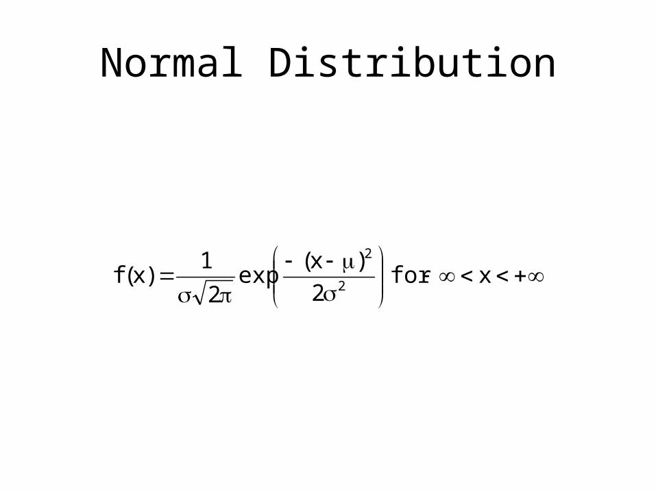
Normal Distribution

xfor

2

)x(exp

2

1)x(f

2

2

Two Normal Distributions

Units of Standard Deviation

Normal Distribution• Approximately 50 percent of all observations fall in the interval μ ±

(2/3)σ.• Approximately 68 percent of all observations fall in the interval μ ±

σ.• Approximately 95 percent of all observations fall in the interval μ ±

2σ.• Approximately 99 percent of all observations fall in the interval μ ±

3σ.• Standard normal distribution has a mean of zero and a standard

deviation of 1. We use Z to denote the standard normal random variable.

• The lognormal distribution is widely used for modeling the probability distribution of asset prices.

X

Z

Two Lognormal Distributions

Statistical Inference• In statistics we are often times interested in obtaining information

about the value of some parameter of a population.• To obtain this information we usually take a smaller subset of the

population and try to draw some conclusions from this sample.• Sampling distribution of a statistic is the distribution of all the distinct

possible values that the statistic can assume when computed from samples of the same size randomly drawn from the same population.

• Cross-sectional data represent observations over individual units at a point in time, as opposed to time series data.

• Time series data is a set of observations on a variable’s outcomes in different time periods.

• Investment analysts commonly work with both time-series and cross-sectional data.

Central Limit Theorem

• The central limit theorem states that for large sample sizes, for any underlying distribution for a random variable, the sampling distribution of the sample mean for that variable will be approximately normal, with mean equal to the population mean for that random variable and variance equal to the population variance of the variable divided by sample size.

Standard Error of the Sample Mean

• For a sample mean calculated from a sample generated from a population with standard deviation σ, the standard error of the sample mean is

– when we know σ.

– If the population standard deviation is unknown we have,

– In practice, the population variance is almost always unknown. To compute the sample standard deviation we use,

n

ss

X

nX

1n

XXs

n

1i

2

i2

Point and Interval Estimates of the Population Mean• An estimator is a formula for estimating a parameter. An estimate is

a particular value that we calculate from a sample by using an estimator.

• An unbiased estimator is one whose expected value equals the parameter it is intended to estimate.

• An unbiased estimator is efficient if no other unbiased estimator of the same population parameter has a sampling distribution with smaller variance.

• A consistent estimator is one for which the probability of estimates is close to the value of the population parameter increases as sample size increases.

• A confidence interval is an interval for which we can assert with a given probability 1 − α, called the degree of confidence, that it will contain the parameter it is intended to estimate.

Confidence Intervals for the Population Mean

• For normally distributed population with known variance.

• For large sample, population variance unknown.

nzX 2/

n

szX 2/

Confidence Intervals for the Population Mean

• Population variance unknown, t-Distribution

• The t-distribution is a symmetrical probability distribution defined by a single parameter known as degrees of freedom (df).

n

stX 2/

Student’s t-Distribution versus the Standard Normal Distribution

Selection of Sample Size

• All else equal, a larger sample size decreases the width of the confidence interval.

size Sample

deviation standard Sample mean sample theoferror Standard

Bias in Sampling

• Sample selection bias is the error of distorting a statistical analysis due to how the samples are collected.

• Look-ahead bias occurs when information that was not available on the test date is used in the estimation.

• Time-period bias occurs when the test is based on a time period that may make the results time-period specific.

• Survivorship bias occurs if companies are excluded from the analysis because they have gone out of business or because of reasons related to poor performance.

• Data mining bias – Data mining is the practice of determining a model by extensive searching through a dataset for statistically significant patterns.

• An out-of-sample test uses a sample that does not overlap the time period(s) of the sample(s) on which a variable, strategy, or model, was developed.

Hypothesis Testing

• Often times we are interested in testing the validity of some statement. – For example, Is the underlying mean return on this

mutual fund different from the underlying mean return on its benchmark?

• Hypothesis testing is part of the branch of statistics known as statistical inference.

• A hypothesis is a statement about one or more populations.

Steps in Hypothesis Testing

1. Stating the hypotheses.

2. Identifying the appropriate test statistic and its probability distribution.

3. Specifying the significance level.

4. Stating the decision rule.

5. Collecting the data and calculating the test statistic.

6. Making the statistical decision.

Null vs. Alternative Hypothesis

• The null hypothesis is the hypothesis to be tested.

• The alternative hypothesis is the hypothesis accepted when the null hypothesis is rejected.

Formulation of Hypotheses

1. H0: θ = θ0 versus HA: θ ≠ θ0

2. H0: θ ≤ θ0 versus HA: θ > θ0

3. H0: θ ≥ θ0 versus HA: θ < θ0

The first formulation is a two-sided test. The other two are

one-sided tests.

Test Statistic

• A test statistic is a quantity, calculated based on a sample, whose value is the basis for deciding whether or not to reject the null hypothesis.

• In reaching a statistical decision, we can make two possible errors: – We may reject a true null hypothesis (a Type I error), or – We may fail to reject a false null hypothesis (a Type II error).

• The level of significance of a test is the probability of a Type I error that we accept in conducting a hypothesis test, is denoted by α.

• The standard approach to hypothesis testing involves specifying a level of significance (probability of Type I error) only.

• The power of a test is the probability of correctly rejecting the null (rejecting the null when it is false).

• A rejection point (critical value) for a test statistic is a value with which the computed test statistic is compared to decide whether to reject or not reject the null hypothesis.

statistic sample theoferror Standard

Hunder parameter population theof Valuestatistic SamplestatisticTest 0

Test Statistic• The p-value is the smallest level of significance at which the null

hypothesis can be rejected.• The smaller the p-value, the stronger the evidence against the null

hypothesis and in favor of the alternative hypothesis.

Hypothesis Tests Concerning the Mean

• Can test that the mean of a population is equal to or differs from some hypothesized value.

• Can test to see if the sample means from two different populations differ.

Tests Concerning a Single Mean• A t-test is usually used to test a hypothesis concerning the value of

a population mean.• If the variance is unknown and the sample is large, or the sample

is small but the population is normally distributed, or approximately normally distributed.

deviation standard samples

mean population theof valueedhypothesiz the

mean sample X

freedom of degrees 1n with statistictt

,wheren/s

Xt

0

1n

01n

Tests Concerning a Single Mean

• If the population sampled is normally distributed with known variance σ2, then the test statistic for a hypothesis test concerning a single population mean, µ, is

deviation standard populationknown

mean population theof valueedhypothesiz the

,wheren/

Xz

0

0

Tests Concerning a Single Mean

• If the population sampled has unknown variance and the sample is large, in place of a t-test, an alternative statistic is

deviation standard populationknown s

,wheren/s

Xz 0

Rejection Points for a z-Test For α = 0.10

1. H0: θ = θ0 verus Ha: θ ≠ θ0 Reject the null hypothesis if z > 1.645 or

if z < -1.645.

2. H0: θ ≤ θ0 verus Ha: θ > θ0 Reject the null hypothesis if z > 1.28

3. H0: θ ≥ θ0 verus Ha: θ < θ0 Reject the null hypothesis if z < -1.28


1. H0: θ = θ0 verus Ha: θ ≠ θ0 Reject the null hypothesis if z > 1.96 or if

z < -1.96.




1. H0: θ = θ0 verus Ha: θ ≠ θ0 Reject the null hypothesis if z > 2.575 or

if z < -2.575



Rejection Points, 0.05 Significance Level, Two-Sided Test of the

Population Mean Using a z-Test

Rejection Point, 0.05 Significance Level, One-Sided Test of the

Population Mean Using a z-Test

Tests Concerning the Differences between Means

• Sometimes we are interested in testing whether the mean value differs between two groups.

• If reasonable to assume– normally distributed– samples are independent

• We can combine observations from both samples to get a pooled estimate of the unknown population variance.

Formulation of Hypotheses

1. H0: µ1 - µ2 = 0 versus HA: µ1 - µ2 ≠ 0

2. H0: µ1 - µ2 ≤ 0 versus HA: µ1 - µ2 > 0

3. H0: µ1 - µ2 ≥ 0 versus HA: µ1 - µ2 < 0

Test Statistic for a Test of Difference between 2 Population Means

• Normally distributed populations, population variances unknown, but assumed to be equal.

– Pooled Estimator of the Common Variance

– degrees of freedom is n1 + n2 - 2

2/1

2

2p

1

2p

2121

n

s

n

s

XXt

2nn

s)1n(s)1n(s

21

222

2112

p

Test Statistic for a Test of Difference between 2 Population Means

• Normally distributed populations, population variances unequal and unknown.

– Degrees of freedom is given by

2/1

2

22

1

21

2121

ns

ns

XXt

2

2

222

1

2

121

2

2

22

1

21

//

n

ns

n

ns

n

s

n

s

df

Mean Differences – Populations Not Independent

• If the samples are not independent, a test of mean difference is done using paired observations.

1. H0: µd = µd0 versus HA: µd ≠ µd0

2. H0: µd ≤ µd0 versus HA: µd > µd0

3. H0: µd ≥ µd0 versus HA: µd < µd0

Mean Differences – Populations Not Independent

• To calculate the t-statistic, we first need to find the sample mean difference:

• The sample variance is

• The standard deviation of the mean is

• The test statistic, with n – 1 df is,

n

ss d

d

n

1iid

n

1d

1n

dds

2n

1ii

2d

d

0d

s

dt

Hypothesis Tests Concerning Variance

• We examine two types: – tests concerning the value of a single population

variance and – tests concerning the differences between two

population variances.

• We can formulate hypotheses as follows:

20

2a

20

20

20

2a

20

20

20

2a

20

20

:H versus:H .3

:H versus:H .2

:H versus:H .1

Tests Concerning the Value of a Population Variance (Normal Dist)

• where,

df 1n ,s)1n(

20

22

1n

XXs

n

1i

2

i2

Tests Concerning the Equality of Two Variances

• We can formulate hypotheses as follows:

• Suppose we have two samples, the first with n1 observations and the second with n2 observations

22

21a

22

210

22

21a

22

210

22

21a

22

210

:H versus:H .3

:H versus:H .2

:H versus:H .1

freedom of degrees )1(n and )1n( with ,s

sF 212

2

21

Nonparametric Inference

• A nonparametric test is not concerned with a parameter or makes minimal assumptions about the population being sampled.

• A nonparametric test is primarily used in three situations: when data do not meet distributional assumptions, when data are given in ranks, or when the hypothesis we are addressing does not concern a parameter.

The Spearman Rank Correlation Coefficient

• The Spearman rank correlation coefficient is calculated on the ranks of two variables within their respective samples.

2/12S

S2/1

2

n

1i

2i

S

r1

r)2n(t

1nn

d61r

Documents

Topic 2: Statistical Concepts and Market Returns