Topic 16: Interval Estimationjwatkins/p-interval.pdf · variables with unknown mean and unknown standard deviation. Let S2 be the unbiased sample variance. If we are ... broader shoulders

Topic 16: Interval Estimation∗

November 10, 2011

Our strategy to estimation thus far has been to use a method to find an estimator, e.g., method of moments, ormaximum likelihood, and evaluate the quality of the estimator by evaluating the bias and the variance of the estimator.Often, we know more about the distribution of the estimator and this allows us to take a more comprehensive statementabout the estimation procedure.

Interval estimation is an alternative to the variety of point estimation techniques we have examined. Given datax, we replace the point estimate θ(x) for the parameter θ by a statistic that is subset C(x) of the parameter space.We will consider both the classical and Bayesian approaches to statistics. As we shall learn, the two approaches havedifferent interpretations for interval estimates.

1 Classical StatisticsIn this case, the random set C(X) has a high probability, γ, of containing the true parameter value θ. In symbols,

Pθ{θ ∈ C(X)} = γ.

−3 −2 −1 0 1 2 30

0.05

0.1

0.15

0.2

0.25

0.3

0.35

0.4

zα

area α

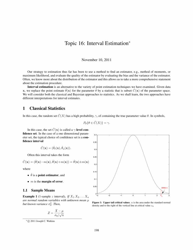
Figure 1: Upper tail critical values. α is the area under the standard normaldensity and to the right of the vertical line at critical value zα

In this case, the set C(x) is called a γ-level con-fidence set. In the case of a one dimensional param-eter set, the typical choice of confidence set is a con-fidence interval

C(x) = (θ`(x), θu(x)).

Often this interval takes the form

C(x) = (θ(x)−m(x), θ(x)+m(x)) = θ(x)±m(x)

where

• θ is a point estimator, and

• m is the margin of error.

1.1 Sample MeansExample 1 (1-sample z interval). If X1.X2. . . . Xn

are normal random variables with unknown mean µbut known variance σ2

0 . Then,

Z =X − µσ0/√n

∗ c© 2011 Joseph C. Watkins

198

Introduction to Statistical Methodology Interval Estimation

is a standard normal random variable. For any α between 0 and 1, let zα satisfy

P{Z > zα} = α or equivalently 1− α = P{Z ≤ zα}.

The value is known as the upper tail probability with critical value zα. We can compute this in R using, for example

> qnorm(0.975)[1] 1.959964

for α = 0.025.If γ = 1− 2α, then α = (1− γ)/2. In this case, we have that

P{−zα < Z < zα} = γ.

If µ0 is the state of nature, then the event

−zα < X−µ0σ0/√n< zα

−zα < µ0−Xσ0/√n< zα

X − zασ0√n< µ0 < X + zα

σ0√n

has probability γ. Thus, for data x,x± z(1−γ)/2

σ0√n

is a confidence interval with confidence level γ. In this case,

µ(x) = x is the estimate for the mean and m(x) = z(1−γ)/2σ0/√n is the margin of error.

We can use the z-interval above for the confidence interval for µ for data that is not necessarily normally dis-tributed as long as the central limit theorem applies. For one population tests for means, n > 30 and data not stronglyskewed is a good rule of thumb.

Generally, the standard deviation is not known and must be estimated. So, let X1, X2, · · · , Xn be normal randomvariables with unknown mean and unknown standard deviation. Let S2 be the unbiased sample variance. If we areforced to replace the unknown standard deviation σ with its unbiased estimate s, then the statistic is known as t:

t =x− µs/√n.

The term s/√n which estimates the standard deviation of the sample mean is called the standard error. The

remarkable discovery by William Gossett is that the distribution of the t statistic can be determined exactly. Write

Tn−1 =√n(X − µ)

S.

Then, Gossett was able to establish the following three facts:

• The numerator is a standard normal random variable.

• The denominator is the square root of

S2 =1

n− 1

n∑i=1

(Xi − X)2.

The sum has chi-square random distribution with n− 1 degrees of freedom.

199


-4 -2 0 2 4

0.0

0.1

0.2

0.3

0.4

x

-4 -2 0 2 4

0.0

0.1

0.2

0.3

0.4

x

-4 -2 0 2 4

0.0

0.2

0.4

0.6

0.8

1.0

x

-4 -2 0 2 4

0.0

0.2

0.4

0.6

0.8

1.0

x

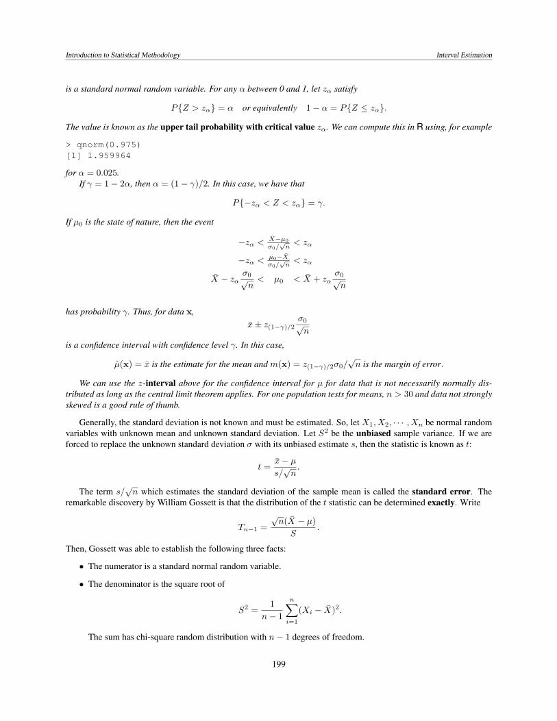
Figure 2: The density and distribution function for a standard normal random variable (black) and a t random variable with 4 degrees of freedom(red). The variance of the t distribution is df/(df − 2) = 4/(4− 2) = 2 is higher than the variance of a standard normal. This can be seen in thebroader shoulders of the density function or in the larger increases in the distribution function away from the mean of 0.

• The numerator and denominator are independent.

With this, Gossett was able to compute the density of the t distribution with n− 1 degrees of freedom.

Again, for any α between 0 and 1, let upper tail probability tn−1,α satisfy

P{Tn−1 > tn−1,α} = α or equivalently P{Tn−1 ≤ tn−1,α} = 1− α.

We can compute this in R using, for example

> qt(0.975,12)[1] 2.178813

for α = 0.025 and n = 12.

Example 2. For the data on the lengths of 200 Bacillus subtilis, we had a mean x = 2.49 and standard deviations = 0.674. For a 96% confidence interval α = 0.02. Thus, we type in R,

> qt(0.98,199)[1] 2.067298

Thus the interval is2.490± 2.0674

0.674√200

= 2.490± 0.099 or (2.391, 2.589)

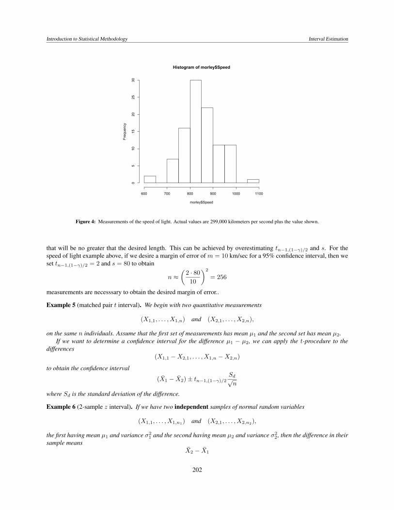
Example 3. We can obtain the data for the Michaelson-Morley experiment using R by typing

> data(morley)

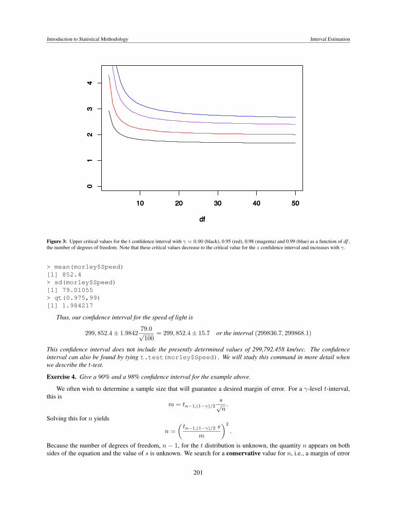
The data have 100 rows - 5 experiments (column 1) of 20 runs (column 2). The Speed is in column 3. The valuesfor speed are the amounts over 299,000 km/sec. Thus, a t-confidence interval will have 99 degrees of freedom. We cansee a histogram by writing hist(morley$Speed). To determine a 95% confidence interval, we find

200


10 20 30 40 50

01

23

4

df

10 20 30 40 50

01

23

4

df

10 20 30 40 50

01

23

4

df

10 20 30 40 50

01

23

4

df

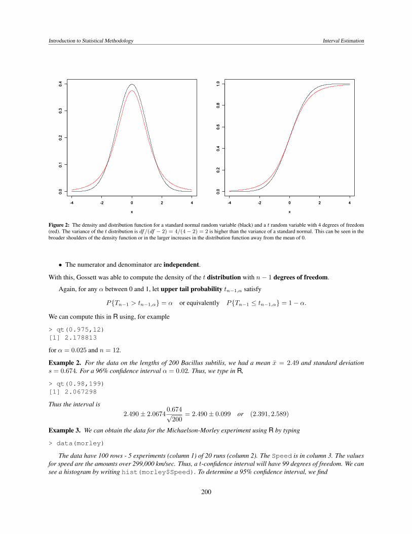
Figure 3: Upper critical values for the t confidence interval with γ = 0.90 (black), 0.95 (red), 0.98 (magenta) and 0.99 (blue) as a function of df ,the number of degrees of freedom. Note that these critical values decrease to the critical value for the z confidence interval and increases with γ.

> mean(morley$Speed)[1] 852.4> sd(morley$Speed)[1] 79.01055> qt(0.975,99)[1] 1.984217

Thus, our confidence interval for the speed of light is

299, 852.4± 1.984279.0√100

= 299, 852.4± 15.7 or the interval (299836.7, 299868.1)

This confidence interval does not include the presently determined values of 299,792.458 km/sec. The confidenceinterval can also be found by tying t.test(morley$Speed). We will study this command in more detail whenwe describe the t-test.

Exercise 4. Give a 90% and a 98% confidence interval for the example above.

We often wish to determine a sample size that will guarantee a desired margin of error. For a γ-level t-interval,this is

m = tn−1,(1−γ)/2s√n.

Solving this for n yields

n =(tn−1,(1−γ)/2 s

m

)2

.

Because the number of degrees of freedom, n − 1, for the t distribution is unknown, the quantity n appears on bothsides of the equation and the value of s is unknown. We search for a conservative value for n, i.e., a margin of error

201


Histogram of morley$Speed

morley$Speed

Frequency

600 700 800 900 1000 1100

05

1015

2025

30

Figure 4: Measurements of the speed of light. Actual values are 299,000 kilometers per second plus the value shown.

that will be no greater that the desired length. This can be achieved by overestimating tn−1,(1−γ)/2 and s. For thespeed of light example above, if we desire a margin of error of m = 10 km/sec for a 95% confidence interval, then weset tn−1,(1−γ)/2 = 2 and s = 80 to obtain

n ≈(

2 · 8010

)2

= 256

measurements are necesssary to obtain the desired margin of error..

Example 5 (matched pair t interval). We begin with two quantitative measurements

(X1,1, . . . , X1,n) and (X2,1, . . . , X2,n),

on the same n individuals. Assume that the first set of measurements has mean µ1 and the second set has mean µ2.If we want to determine a confidence interval for the difference µ1 − µ2, we can apply the t-procedure to the

differences(X1,1 −X2,1, . . . , X1,n −X2,n)

to obtain the confidence interval

(X1 − X2)± tn−1,(1−γ)/2Sd√n

where Sd is the standard deviation of the difference.

Example 6 (2-sample z interval). If we have two independent samples of normal random variables

(X1,1, . . . , X1,n1) and (X2,1, . . . , X2,n2),

the first having mean µ1 and variance σ21 and the second having mean µ2 and variance σ2

2 , then the difference in theirsample means

X2 − X1

202


is also a normal random variable with

mean µ1 − µ2 and varianceσ2

1

n1+σ2

2

n2.

Therefore,

Z =(X1 − X2)− (µ1 − µ2)√

σ21n1

+ σ22n2

is a standard normal random variable. This gives us a confidence interval for the difference in parameters µ1 − µ2.

(X1 − X2)± z(1−γ)/2

√σ2

1

n1+σ2

2

n2.

Example 7 (2-sample t interval). If we know that σ21 = σ2

2 , then we can pool the data to compute the standarddeviation. Let S2

1 and S22 be the sample variances from the two samples. Then the pooled sample variance Sp is the

weighted average of the sample variances with weights equal to their respective degrees of freedom.

S2p =

(n1 − 1)S21 + (n2 − 1)S2

2

n1 + n2 − 2.

This give a statistic

Tn1+n2−2 =(X1 − X2)− (µ1 − µ2)

Sp

√1n1

+ 1n2

that has a t distribution with n1 + n2 − 2 degrees of freedom. Thus we have the γ confidence interval

(X1 − X2)± tn1+n2−2,(1−γ)/2Sp

√1n1

+1n2

for µ1 − µ2.If we do not know that σ2

1 = σ22 , then the corresponding standardized random variable

T =(X1 − X2)− (µ1 − µ2)√

S21n1

+ S22n2

no longer has a t-distribution.Welch and Satterthwaite have provided an approximation to the t distribution with effective degrees of freedom

ν =

(s21n1

+ s22n2

)2

s41n2

1·(n1−1)+ s42

n22·(n2−1)

. (1)

For two sample tests, the number of observations per group may need to be at least 40 for a good approximationto the normal distribution.

Exercise 8. Show that the effective degrees is between the worst case of the minimum choice from a one samplet-interval and the best case of equal variances.

min{n1, n2} − 1 ≤ ν ≤ n1 + n2 − 2

203


1.2 Linear RegressionFor ordinary linear regression, we have given least squares estimates for the slope β and the intercept α. For data(x1, y1), (x2, y2(. . . , (xn, yn), our model is

yi = α+ βxi + εi

where εi are independent N(0, σ) random variables. Recall that the estimator for the slope

β(x, y) =cov(x, y)

var(x)

is unbiased.

Exercise 9. Show that the variance of β equals σ2/(n− 1)var(x).

If σ is known, this suggests a z-interval for a γ-level confidence interval

β ± z(1−γ)/2σ

sx√n− 1

.

Generally, σ is unknown. However, the variance of the residuals,

s2U =

1n− 2

n∑i=1

(yi − (α− βx))2 (2)

is an unbiased estimator of σ2 and sU/σ has a t distribution with n− 2 degrees of freedom. This gives the t-interval

β ± tn−2,(1−γ)/2sU

sx√n− 1

.

As the formula shows, the margin of error is proportional to the standard deviation of the residuals. It is inverselyproportional to the standard deviation of the x measurement. Thus, we can reduce the margin of error by taking abroader set of values for the explanatory variables.

For the data on the humerus and femur of the five specimens of Archeopteryx, we have β = 1.197. σU = 1.982,sx = 13.2, and t3,0.025 = 3.1824, Thus, the 95% confidence interval is 1.197± 0.239 or (0.958, 1.436).

1.3 Sample ProportionsExample 10 (proportions). For n Bernoulli trials with success parameter p, the sample proportion p has

mean p and variancep(1− p)

n.

The parameter p appears in both the mean and in the variance. Thus, we need to make a choice p to replace p in theconfidence interval

p± z(1−γ)/2

√p(1− p)

n. (3)

One simple choice for p is p. Based on extensive numerical experimentation, one more recent popular choice is

p =x+ 2n+ 4

where x is the number of successes.For population proportions, we ask that the mean number of successes np and the mean number of failures

n(1− p) each be at least 10. We have this requirement so that a normal random variable is a good approximation tothe appropriate binomial random variable.

204


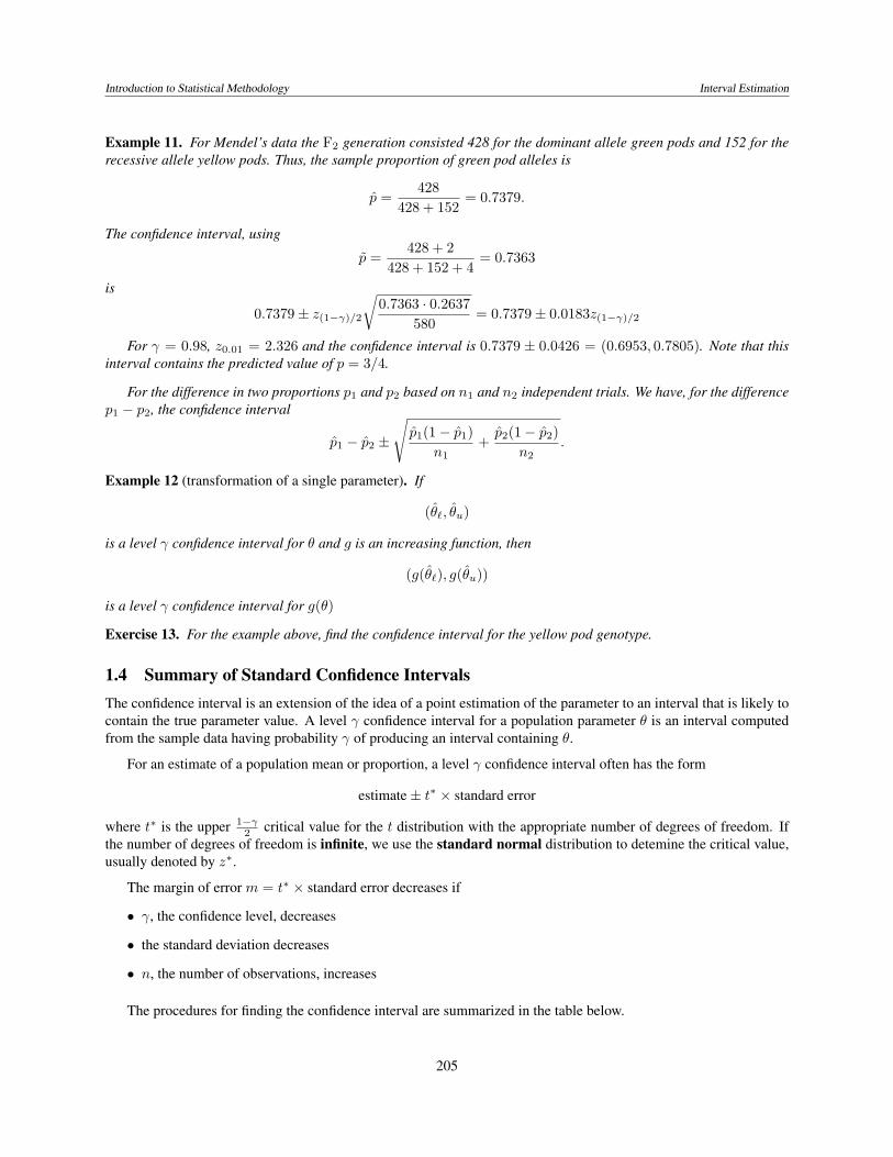
Example 11. For Mendel’s data the F2 generation consisted 428 for the dominant allele green pods and 152 for therecessive allele yellow pods. Thus, the sample proportion of green pod alleles is

p =428

428 + 152= 0.7379.

The confidence interval, using

p =428 + 2

428 + 152 + 4= 0.7363

is

0.7379± z(1−γ)/2

√0.7363 · 0.2637

580= 0.7379± 0.0183z(1−γ)/2

For γ = 0.98, z0.01 = 2.326 and the confidence interval is 0.7379 ± 0.0426 = (0.6953, 0.7805). Note that thisinterval contains the predicted value of p = 3/4.

For the difference in two proportions p1 and p2 based on n1 and n2 independent trials. We have, for the differencep1 − p2, the confidence interval

p1 − p2 ±

√p1(1− p1)

n1+p2(1− p2)

n2.

Example 12 (transformation of a single parameter). If

(θ`, θu)

is a level γ confidence interval for θ and g is an increasing function, then

(g(θ`), g(θu))

is a level γ confidence interval for g(θ)

Exercise 13. For the example above, find the confidence interval for the yellow pod genotype.

1.4 Summary of Standard Confidence IntervalsThe confidence interval is an extension of the idea of a point estimation of the parameter to an interval that is likely tocontain the true parameter value. A level γ confidence interval for a population parameter θ is an interval computedfrom the sample data having probability γ of producing an interval containing θ.

For an estimate of a population mean or proportion, a level γ confidence interval often has the form

estimate± t∗ × standard error

where t∗ is the upper 1−γ2 critical value for the t distribution with the appropriate number of degrees of freedom. If

the number of degrees of freedom is infinite, we use the standard normal distribution to detemine the critical value,usually denoted by z∗.

The margin of error m = t∗ × standard error decreases if

• γ, the confidence level, decreases

• the standard deviation decreases

• n, the number of observations, increases

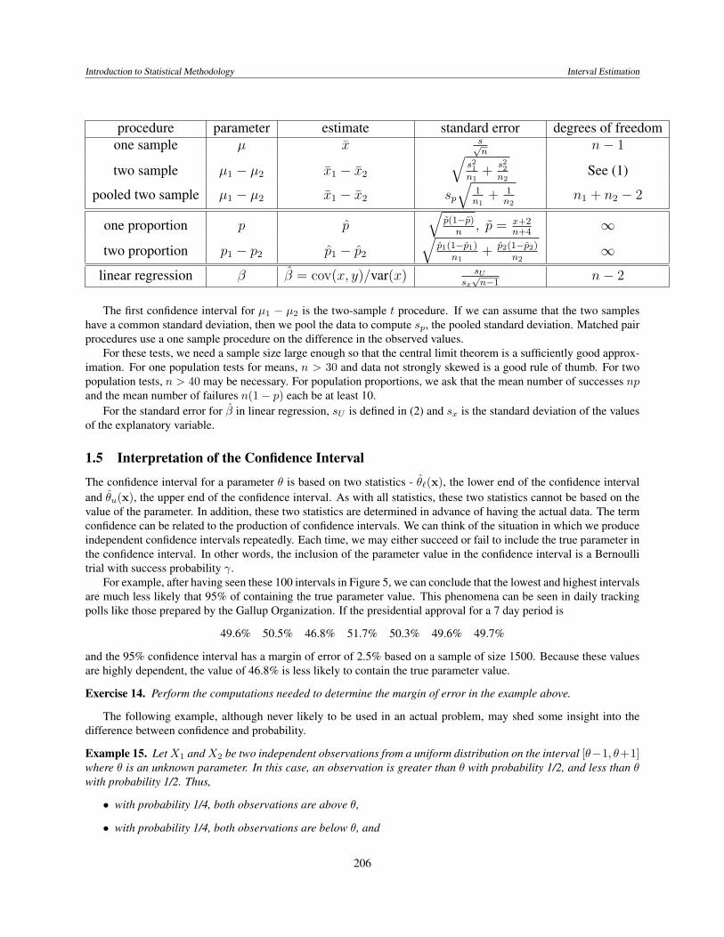
The procedures for finding the confidence interval are summarized in the table below.

205


procedure parameter estimate standard error degrees of freedomone sample µ x s√

nn− 1

two sample µ1 − µ2 x1 − x2

√s21n1

+s22n2

See (1)

pooled two sample µ1 − µ2 x1 − x2 sp√

1n1

+ 1n2

n1 + n2 − 2

one proportion p p√

p(1−p)n

, p = x+2n+4

∞

two proportion p1 − p2 p1 − p2

√p1(1−p1)

n1+ p2(1−p2)

n2∞

linear regression β β = cov(x, y)/var(x) sUsx√n−1

n− 2

The first confidence interval for µ1 − µ2 is the two-sample t procedure. If we can assume that the two sampleshave a common standard deviation, then we pool the data to compute sp, the pooled standard deviation. Matched pairprocedures use a one sample procedure on the difference in the observed values.

For these tests, we need a sample size large enough so that the central limit theorem is a sufficiently good approx-imation. For one population tests for means, n > 30 and data not strongly skewed is a good rule of thumb. For twopopulation tests, n > 40 may be necessary. For population proportions, we ask that the mean number of successes npand the mean number of failures n(1− p) each be at least 10.

For the standard error for β in linear regression, sU is defined in (2) and sx is the standard deviation of the valuesof the explanatory variable.

1.5 Interpretation of the Confidence Interval

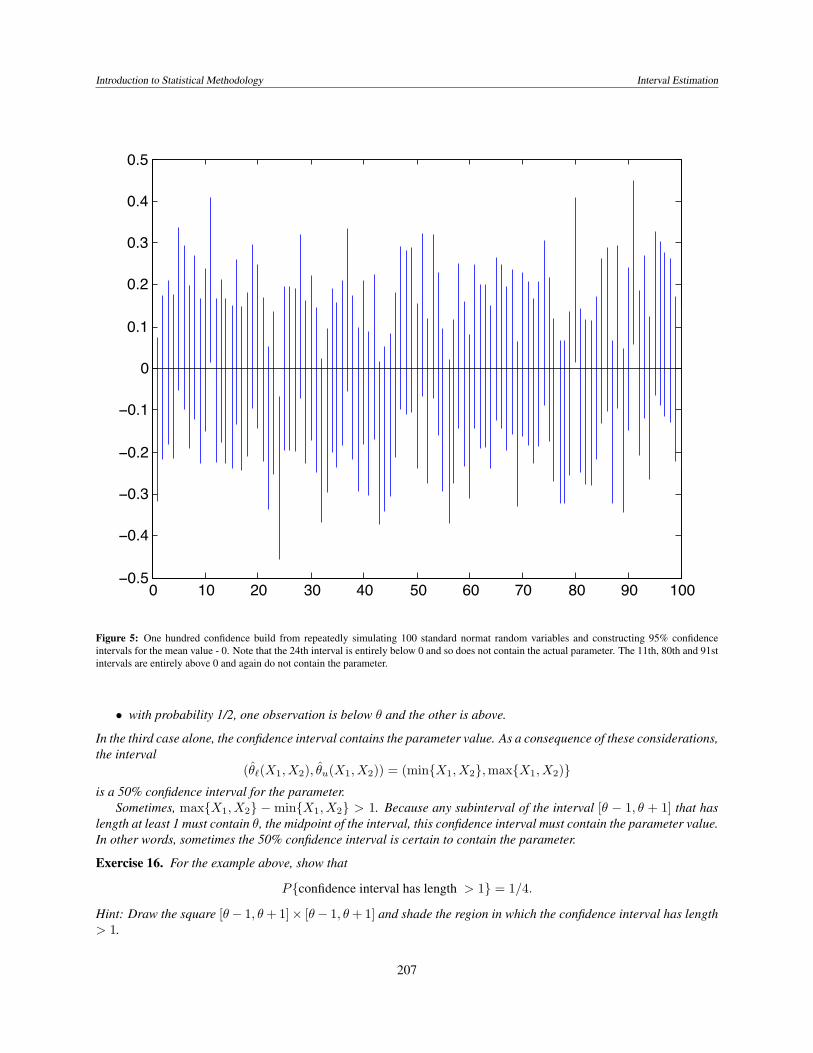
The confidence interval for a parameter θ is based on two statistics - θ`(x), the lower end of the confidence intervaland θu(x), the upper end of the confidence interval. As with all statistics, these two statistics cannot be based on thevalue of the parameter. In addition, these two statistics are determined in advance of having the actual data. The termconfidence can be related to the production of confidence intervals. We can think of the situation in which we produceindependent confidence intervals repeatedly. Each time, we may either succeed or fail to include the true parameter inthe confidence interval. In other words, the inclusion of the parameter value in the confidence interval is a Bernoullitrial with success probability γ.

For example, after having seen these 100 intervals in Figure 5, we can conclude that the lowest and highest intervalsare much less likely that 95% of containing the true parameter value. This phenomena can be seen in daily trackingpolls like those prepared by the Gallup Organization. If the presidential approval for a 7 day period is

49.6% 50.5% 46.8% 51.7% 50.3% 49.6% 49.7%

and the 95% confidence interval has a margin of error of 2.5% based on a sample of size 1500. Because these valuesare highly dependent, the value of 46.8% is less likely to contain the true parameter value.

Exercise 14. Perform the computations needed to determine the margin of error in the example above.

The following example, although never likely to be used in an actual problem, may shed some insight into thedifference between confidence and probability.

Example 15. LetX1 andX2 be two independent observations from a uniform distribution on the interval [θ−1, θ+1]where θ is an unknown parameter. In this case, an observation is greater than θ with probability 1/2, and less than θwith probability 1/2. Thus,

• with probability 1/4, both observations are above θ,

• with probability 1/4, both observations are below θ, and

206


0 10 20 30 40 50 60 70 80 90 100−0.5

−0.4

−0.3

−0.2

−0.1

0

0.1

0.2

0.3

0.4

0.5

Figure 5: One hundred confidence build from repeatedly simulating 100 standard normat random variables and constructing 95% confidenceintervals for the mean value - 0. Note that the 24th interval is entirely below 0 and so does not contain the actual parameter. The 11th, 80th and 91stintervals are entirely above 0 and again do not contain the parameter.

• with probability 1/2, one observation is below θ and the other is above.

In the third case alone, the confidence interval contains the parameter value. As a consequence of these considerations,the interval

(θ`(X1, X2), θu(X1, X2)) = (min{X1, X2},max{X1, X2)}is a 50% confidence interval for the parameter.

Sometimes, max{X1, X2} − min{X1, X2} > 1. Because any subinterval of the interval [θ − 1, θ + 1] that haslength at least 1 must contain θ, the midpoint of the interval, this confidence interval must contain the parameter value.In other words, sometimes the 50% confidence interval is certain to contain the parameter.

Exercise 16. For the example above, show that

P{confidence interval has length > 1} = 1/4.

Hint: Draw the square [θ− 1, θ+ 1]× [θ− 1, θ+ 1] and shade the region in which the confidence interval has length> 1.

207


1.6 Extensions on the Use of Confidence Intervals

Example 17 (delta method). For estimating the distribution µ by the sample mean X , the delta method provides analternative for the example above. In this case, the standard deviation of g(X) is approximately

|g′(µ)|σ√n

.

We replace µ with X to obtain the confidence interval for g(µ)

g(X)± zα/2|g′(X)|σ√

n.

Using the notation for the example of estimating α3, the coefficient of volume expansion based on independentlength measurements, Y1, Y2, . . . , Yn measured at temperature T1 of an object having length `0 at temperature T0.

Y 3 − `30`30|T1 − T0|

± zα/23Y 2σYn

For multiple independent samples, the simple idea using the transformation in the Example 12 no longer works.For example, to determine the confidence interval using X1 and X2 above, the confidence interval for g(µ1, µ2), thedelta methos gives the confidence interval

g(X1, X2)± zα/2

√(∂

∂xg(X1, X2)

)2σ2

1

n1+(∂

∂yg(X1, X2)

)2σ2

2

n2.

A comparable formula gives confidence intervals based on more than two independent samples

Example 18. Let’s return to the example of n` and nh measurements x and y of, respectively, the length ` and theheight h of a right triangle with the goal of giving the angle

θ = g(`, h) = tan−1

(`

h

)between these two sides. Here are the measurements:

> x[1] 10.224484 10.061800 9.945213 9.982061 9.961353 10.173944 9.952279 9.855147[9] 9.737811 9.956345

> y[1] 4.989871 5.090002 5.021615 4.864633 5.024388 5.123419 5.033074 4.750892 4.985719

[10] 4.912719 5.027048 5.055755> mean(x);sd(x)[1] 9.985044[1] 0.1417969> mean(y);sd(y)[1] 4.989928[1] 0.1028745

The angle θ is the arctangent, here estimated using the mean and given in radians

>(thetahat<-atan(mean(y)/mean(x)))[1] 0.4634398

208


Using the delta method, we have estimated the standard deviation of these measurements.

σθ ≈1

h2 + `2

√h2σ2`

n`+ `2

σ2h

nh.

We estimate this with the sample means and standard deviations

sθ ≈1

y2 + x2

√y2s2x

n`+ x2

s2y

nh= 0.0030.

This gives a γ level z- confidence intervalθ ± z(1−γ)/2sθ.

For a 95% confidence interval, this is 0.4634± 0.0059 = (0.4575, 0.4693) radians or (26.22◦, 26.89◦).We can extend the Welch and Satterthwaite method to include the delta method to create a t-interval with effective

degrees of freedom

ν =

(∂g(x,y)2

∂xs21n1

+ ∂g(x,y)2

∂ys22n2

)2

∂g(x,y)4

∂xs41

n21·(n1−1)

+ ∂g(x,y)4

∂ys42

n22·(n2−1)

.

We compute to find that ν = 19.4 and then use the t-interval

θ ± tν,(1−γ)/2sθ.

For a 95% confidence, this is sightly larger interval 0.4634±0.0063 = (0.4571, 0.4697) radians or (26.19◦, 26.91◦).

Example 19 (maximum likelihood estimation). The Fisher information is the main tool used to set an confidenceinterval for a maximum likelihood estimation. Two choices are typical. First, we can use the Fisher information In(θ).Of course, the estimator is for the unknown value of the parameter θ. This give an confidence interval

θ ± zα/21√nI(θ)

.

More recently, the more popular method is to use the observed information based on the observations x =(x1, x2, . . . , xn).

J(θ) = − ∂2

∂θ2logL(θ|x) = −

n∑i=1

∂2

∂θ2log fX(xi|θ).

This is the second derivative of the score function evaluated at the maximum likelihood estimator. Then, the confidenceinterval is

θ ± zα/21√J(θ)

.

Note that EθJ(θ) = nI(θ), the Fisher information for n observations. Thus, by the law of large numbers

1nJ(θ)→ I(θ) as n→∞.

If the estimator is consistent and I is continuous at θ, then

1nJ(θ)→ I(θ) as n→∞.

209


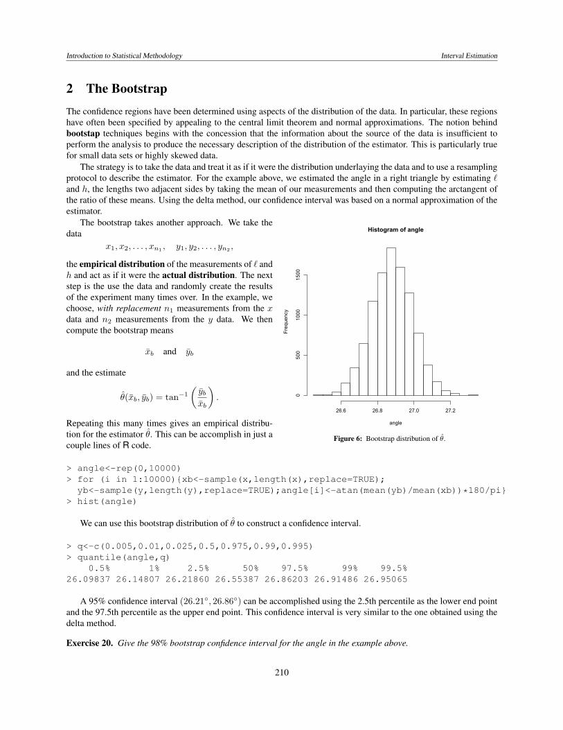
2 The BootstrapThe confidence regions have been determined using aspects of the distribution of the data. In particular, these regionshave often been specified by appealing to the central limit theorem and normal approximations. The notion behindbootstap techniques begins with the concession that the information about the source of the data is insufficient toperform the analysis to produce the necessary description of the distribution of the estimator. This is particularly truefor small data sets or highly skewed data.

The strategy is to take the data and treat it as if it were the distribution underlaying the data and to use a resamplingprotocol to describe the estimator. For the example above, we estimated the angle in a right triangle by estimating `and h, the lengths two adjacent sides by taking the mean of our measurements and then computing the arctangent ofthe ratio of these means. Using the delta method, our confidence interval was based on a normal approximation of theestimator.

Histogram of angle

angle

Frequency

26.6 26.8 27.0 27.2

0500

1000

1500

Figure 6: Bootstrap distribution of θ.

The bootstrap takes another approach. We take thedata

x1, x2, . . . , xn1 , y1, y2, . . . , yn2 ,

the empirical distribution of the measurements of ` andh and act as if it were the actual distribution. The nextstep is the use the data and randomly create the resultsof the experiment many times over. In the example, wechoose, with replacement n1 measurements from the xdata and n2 measurements from the y data. We thencompute the bootstrap means

xb and yb

and the estimate

θ(xb, yb) = tan−1

(ybxb

).

Repeating this many times gives an empirical distribu-tion for the estimator θ. This can be accomplish in just acouple lines of R code.

> angle<-rep(0,10000)> for (i in 1:10000){xb<-sample(x,length(x),replace=TRUE);

yb<-sample(y,length(y),replace=TRUE);angle[i]<-atan(mean(yb)/mean(xb))*180/pi}> hist(angle)

We can use this bootstrap distribution of θ to construct a confidence interval.

> q<-c(0.005,0.01,0.025,0.5,0.975,0.99,0.995)> quantile(angle,q)

0.5% 1% 2.5% 50% 97.5% 99% 99.5%26.09837 26.14807 26.21860 26.55387 26.86203 26.91486 26.95065

A 95% confidence interval (26.21◦, 26.86◦) can be accomplished using the 2.5th percentile as the lower end pointand the 97.5th percentile as the upper end point. This confidence interval is very similar to the one obtained using thedelta method.

Exercise 20. Give the 98% bootstrap confidence interval for the angle in the example above.

210


0.0 0.2 0.4 0.6 0.8 1.0

01

23

4

x

0.0 0.2 0.4 0.6 0.8 1.0

01

23

4

x

0.0 0.2 0.4 0.6 0.8 1.0

01

23

4

0.0 0.2 0.4 0.6 0.8 1.0

01

23

4

0.0 0.2 0.4 0.6 0.8 1.0

01

23

4

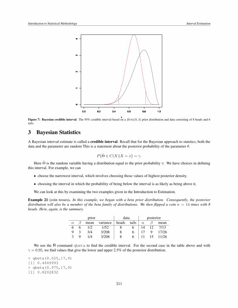
Figure 7: Bayesian credible interval. The 95% credible interval based on a Beta(9, 3) prior distribution and data consisting of 8 heads and 6tails.

3 Bayesian StatisticsA Bayesian interval estimate is called a credible interval. Recall that for the Bayesian approach to statstics, both thedata and the parameter are random This is a statement about the posterior probability of the parameter θ.

P{Θ ∈ C(X)|X = x} = γ.

Here Θ is the random variable having a distribution equal to the prior probability π. We have choices in definingthis interval. For example, we can

• choose the narrowest interval, which involves choosing those values of highest posterior density.

• choosing the interval in which the probability of being below the interval is as likely as being above it.

We can look at this by examining the two examples given in the Introduction to Estimation.

Example 21 (coin tosses). In this example, we began with a beta prior distribution. Consequently, the posteriordistribution will also be a member of the beta family of distributions. We then flipped a coin n = 14 times with 8heads. Here, again, is the summary.

prior data posteriorα β mean variance heads tails α β mean6 6 1/2 1/52 8 6 14 12 7/139 3 3/4 3/208 8 6 17 9 17/263 9 1/4 3/208 8 6 11 15 11/26

We use the R command qbeta to find the credible interval. For the second case in the table above and withγ = 0.95, we find values that give the lower and upper 2.5% of the posterior distribution.

> qbeta(0.025,17,9)[1] 0.4649993> qbeta(0.975,17,9)[1] 0.8202832

211


This gives a 95% credible interval of (0.465, 0.820). This is indicated in the figure above by the two vertical lines.Thus, the area under the density function from the vertical lines outward totals 5%.

Example 22. For the example having both a normal prior distribution and normal data, we find that we also have anormal posterior distribution. In particular, if the prior is normal, mean θ0, variance 1/λ and our data has samplemean x and each observation has variance 1.

The the posterior distribution has mean

θ1(x) =λ

λ+ nθ0 +

n

λ+ nx.

and variance 1/(n+ λ). Thus the credible interval is

θ1(x)± zα/21√λ+ n

.

4 Answers to Selected Exercises3. Using R to find upper tail probabilities, we find that

> qt(0.95,99)[1] 1.660391> qt(0.99,99)[1] 2.364606

For the 90% confidence interval

299, 852.4± 1.660479.0√100

= 299852.4± 13.1 or the interval (299839.3, 299865.5).

For the 98% confidence interval

299, 852.4± 2.364679.0√100

= 299852.4± 18.7 or the interval (299833.7, 299871.1).

8. Let

c =s2

1/n1

s22/n2

. Then,s2

2

n2= c

s21

n1.

Then, substitute for s22/n2 and divide by s2

1/n1 to obtain

ν =

(s21n1

+ s22n2

)2

s41n2

1·(n1−1)+ s42

n22·(n2−1)

=

(s21n1

+ cs21n1

)2

s41n2

1·(n1−1)+ c2s41

n21·(n2−1)

=(1 + c)2

1n1−1 + c2

n2−1

=(n1 − 1)(n2 − 1)(1 + c)2

(n2 − 1) + (n1 − 1)c2.

Take a derivative to see that

dν

dc= (n1 − 1)(n2 − 1)

((n2 − 1) + (n1 − 1)c2) · 2(1 + c)− (1 + c)2 · 2(n1 − 1)c((n2 − 1) + (n1 − 1)c2)2

= 2(n1 − 1)(n2 − 1)(1 + c)((n2 − 1) + (n1 − 1)c2)− (1 + c)(n1 − 1)c

((n2 − 1) + (n1 − 1)c2)2

= 2(n1 − 1)(n2 − 1)(1 + c)(n2 − 1)− (n1 − 1)c

((n2 − 1) + (n1 − 1)c2)2

212


So the maximum takes place at c = (n2 − 1)/(n1 − 1) with value n1 + n2 − 2. Note that for this value

s21

s22

=n1

n2c =

n1/(n1 − 1)n2/(n2 − 1)

and the variances are nearly equal. Notice that this is a global maximum with

ν → n1 − 1 as c→ 0 and s1 � s2 and ν → n2 − 1 as c→∞ and s2 � s1.

The smaller of these two limits is the global minimum.

9. We first determine, E(α,β)[(β − β)2], the variance of β.

β(x, y)− β =1

(n− 1)var(x)

(n∑i=1

(xi − x)(yi − y)− βn∑i=1

(xi − x)(xi − x)

)

=1

(n− 1)var(x)

(n∑i=1

(xi − x)(yi − y − β(xi − x)

)

=1

(n− 1)var(x)

(n∑i=1

(xi − x)((yi − βxi)− (y − βx))

)

=1

(n− 1)var(x)

(n∑i=1

(xi − x)(yi − βxi)−n∑i=1

(xi − x)(y − βx)

)The second sum is 0. For the first, we use the fact that yi − βxi = α+ εi. Thus,

Var(α,β)(β) = Var(α,β)

(1

(n− 1)var(x)

n∑i=1

(xi − x)(α+ εi)

)=

1(n− 1)2var(x)2

n∑i=1

(xi − x)2Var(α,β)(α+ εi)

=1

(n− 1)2var(x)2

n∑i=1

(xi − x)2σ2 =σ2

(n− 1)var(x)

13. The confidence interval for the proportion yellow pod genes 1−p is (0.2195, 0.3047). The proportion of yellow podphenotype is (1−p)2 and a 95% confidence interval has as its endpoints the square of these numbers - (0.0482, 0.0928).

14. The critical value z0.025 = 1.96. For p = 0.468 and n = 1500, the number of successes is x = 702. The marginof error is

z0.025

√p(1− p)

n= 0.025.

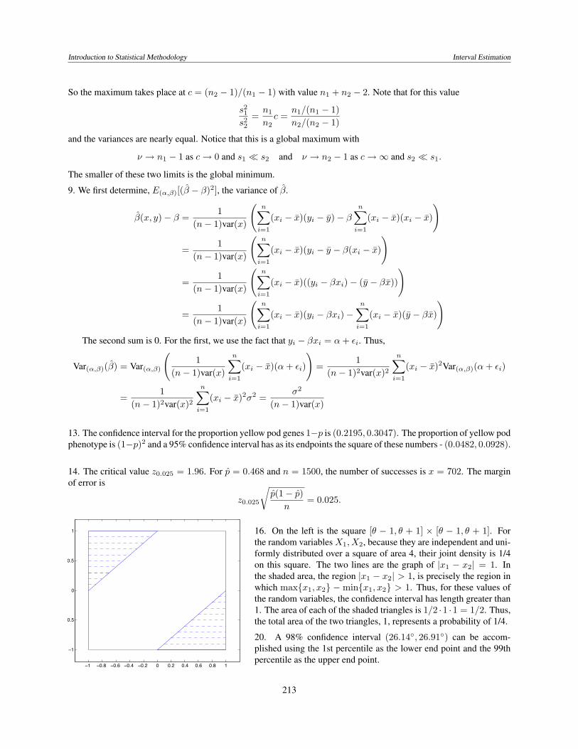
−1 −0.8 −0.6 −0.4 −0.2 0 0.2 0.4 0.6 0.8 1

−1

−0.5

0

0.5

1 16. On the left is the square [θ − 1, θ + 1] × [θ − 1, θ + 1]. Forthe random variables X1, X2, because they are independent and uni-formly distributed over a square of area 4, their joint density is 1/4on this square. The two lines are the graph of |x1 − x2| = 1. Inthe shaded area, the region |x1 − x2| > 1, is precisely the region inwhich max{x1, x2} − min{x1, x2} > 1. Thus, for these values ofthe random variables, the confidence interval has length greater than1. The area of each of the shaded triangles is 1/2 ·1 ·1 = 1/2. Thus,the total area of the two triangles, 1, represents a probability of 1/4.

20. A 98% confidence interval (26.14◦, 26.91◦) can be accom-plished using the 1st percentile as the lower end point and the 99thpercentile as the upper end point.

213

Documents

Topic 16: Interval Estimationjwatkins/p-interval.pdf · variables with unknown mean and unknown standard deviation. Let S2 be the unbiased sample variance. If we are ... broader shoulders