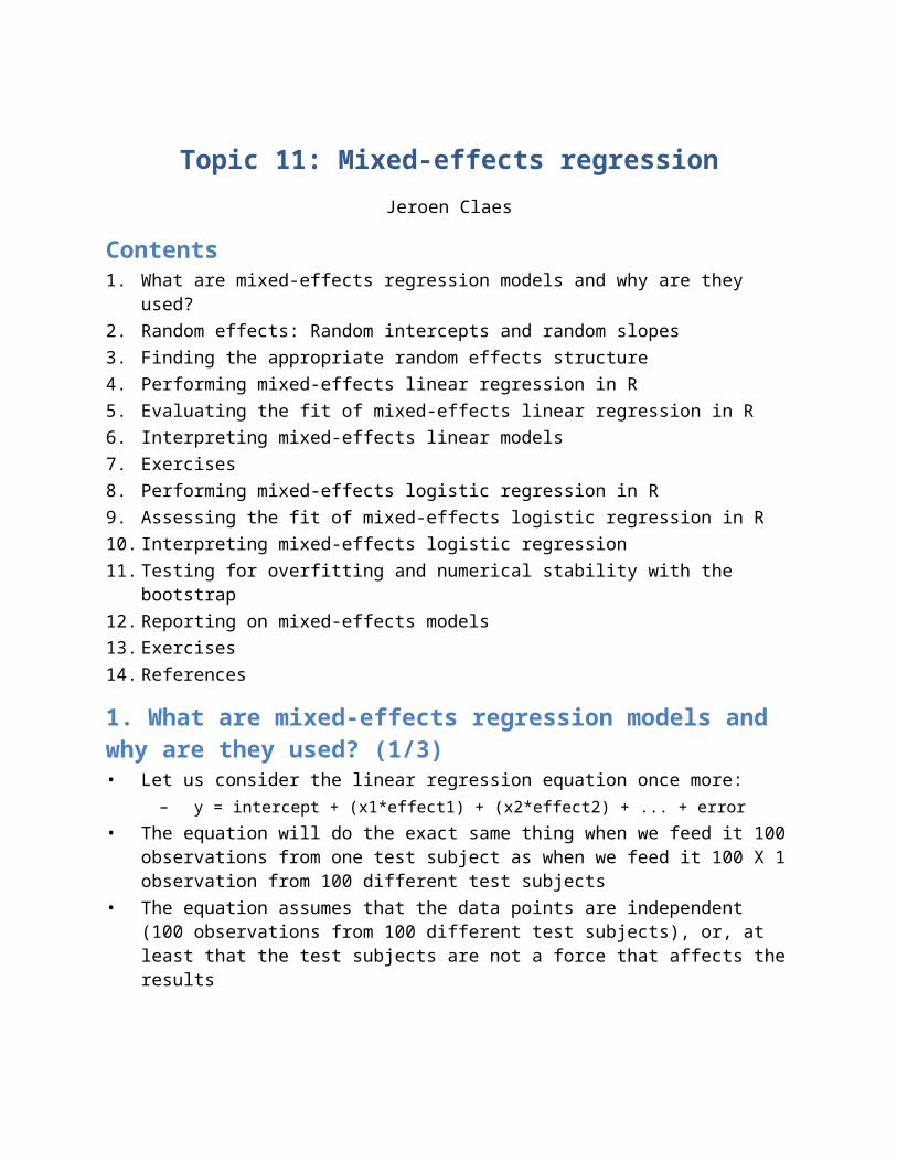
Topic 11: Mixed-effects regressionJeroen Claes

Contents1. What are mixed-effects regression models and why are they used?2. Random effects: Random intercepts and random slopes3. Finding the appropriate random effects structure4. Performing mixed-effects linear regression in R5. Evaluating the fit of mixed-effects linear regression in R6. Interpreting mixed-effects linear models7. Exercises8. Performing mixed-effects logistic regression in R9. Assessing the fit of mixed-effects logistic regression in R10. Interpreting mixed-effects logistic regression11. Testing for overfitting and numerical stability with the bootstrap12. Reporting on mixed-effects models13. Exercises14. References

1. What are mixed-effects regression models and why are they used? (1/3)• Let us consider the linear regression equation once more:

– y = intercept + (x1*effect1) + (x2*effect2) + ... + error• The equation will do the exact same thing when we feed it 100 observations from one

test subject as when we feed it 100 X 1 observation from 100 different test subjects• The equation assumes that the data points are independent (100 observations from

100 different test subjects), or, at least that the test subjects are not a force that affects the results

1. What are mixed-effects regression models and why are they used? (2/3)• Unfortunately, test subjects do affect the results and we should correct for that• More generally, we want to make sure that our analysis generalizes from our sample

to the population it represents• Therefore, we want to have a way of adjusting our model for those aspects of our

investigation that will not be the same when we collect new data• This way, we can measure the effects of our independent variables more precisely and

we can be more sure that the effects that we find are not due to the atypical nature of some aspects of our data

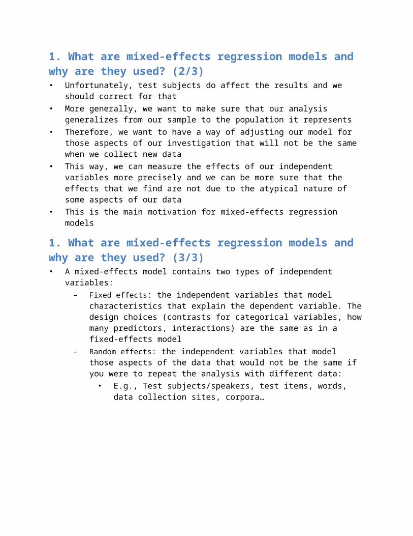
• This is the main motivation for mixed-effects regression models

1. What are mixed-effects regression models and why are they used? (3/3)• A mixed-effects model contains two types of independent variables:

– Fixed effects: the independent variables that model characteristics that explain the dependent variable. The design choices (contrasts for categorical variables, how many predictors, interactions) are the same as in a fixed-effects model

– Random effects: the independent variables that model those aspects of the data that would not be the same if you were to repeat the analysis with different data:

• E.g., Test subjects/speakers, test items, words, data collection sites, corpora…

2. Random effects: Random intercepts and random slopes

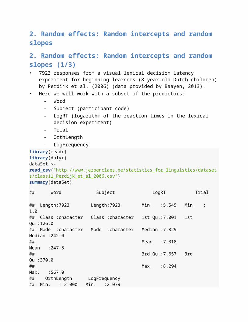
2. Random effects: Random intercepts and random slopes (1/3)• 7923 responses from a visual lexical decision latency experiment for beginning

learners (8 year-old Dutch children) by Perdijk et al. (2006) (data provided by Baayen, 2013).

• Here we will work with a subset of the predictors:– Word– Subject (participant code)– LogRT (logarithm of the reaction times in the lexical decision experiment)– Trial– OrthLength– LogFrequency

library(readr)library(dplyr)dataSet <- read_csv("http://www.jeroenclaes.be/statistics_for_linguistics/datasets/class11_Perdijk_et_al_2006.csv")summary(dataSet)

## Word Subject LogRT Trial

## Length:7923 Length:7923 Min. :5.545 Min. : 1.0 ## Class :character Class :character 1st Qu.:7.001 1st Qu.:126.0 ## Mode :character Mode :character Median :7.329 Median :242.0 ## Mean :7.318

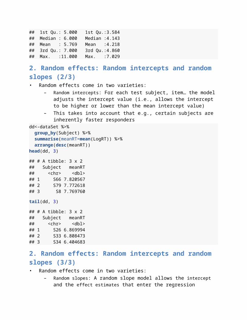
Mean :247.8 ## 3rd Qu.:7.657 3rd Qu.:370.0 ## Max. :8.294 Max. :567.0 ## OrthLength LogFrequency ## Min. : 2.000 Min. :2.079 ## 1st Qu.: 5.000 1st Qu.:3.584 ## Median : 6.000 Median :4.143 ## Mean : 5.769 Mean :4.218 ## 3rd Qu.: 7.000 3rd Qu.:4.860 ## Max. :11.000 Max. :7.029

2. Random effects: Random intercepts and random slopes (2/3)• Random effects come in two varieties:

– Random intercepts: For each test subject, item… the model adjusts the intercept value (i.e., allows the intercept to be higher or lower than the mean intercept value)

– This takes into account that e.g., certain subjects are inherently faster responders

dd<-dataSet %>% group_by(Subject) %>% summarise(meanRT=mean(LogRT)) %>% arrange(desc(meanRT))head(dd, 3)

## # A tibble: 3 x 2## Subject meanRT## <chr> <dbl>## 1 S66 7.820567## 2 S79 7.772618## 3 S8 7.769760

tail(dd, 3)

## # A tibble: 3 x 2## Subject meanRT## <chr> <dbl>## 1 S26 6.869994## 2 S33 6.808473## 3 S34 6.404683

2. Random effects: Random intercepts and random slopes (3/3)• Random effects come in two varieties:

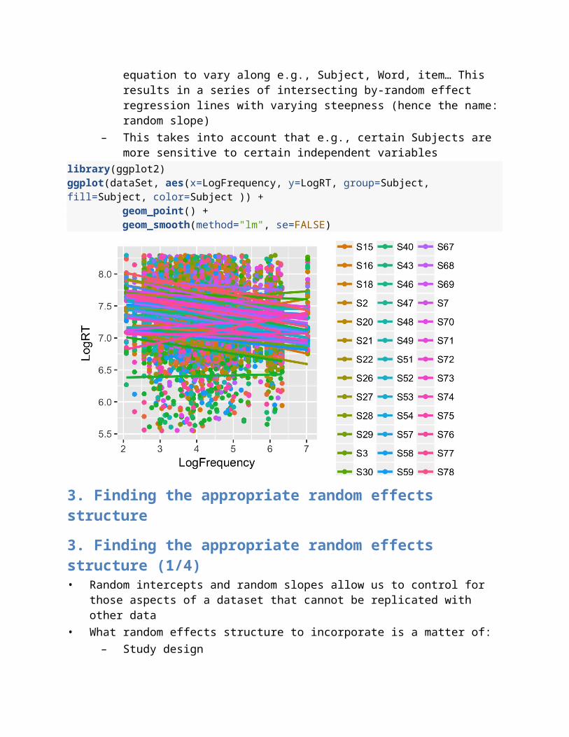
– Random slopes: A random slope model allows the intercept and the effect estimates that enter the regression equation to vary along e.g., Subject, Word, item… This results in a series of intersecting by-random effect regression lines with varying steepness (hence the name: random slope)

– This takes into account that e.g., certain Subjects are more sensitive to certain independent variables

library(ggplot2)ggplot(dataSet, aes(x=LogFrequency, y=LogRT, group=Subject, fill=Subject, color=Subject )) + geom_point() + geom_smooth(method="lm", se=FALSE)

3. Finding the appropriate random effects structure

3. Finding the appropriate random effects structure (1/4)• Random intercepts and random slopes allow us to control for those aspects of a

dataset that cannot be replicated with other data• What random effects structure to incorporate is a matter of:

– Study design– Emperical adequacy and statistical power of the dataset

3. Finding the appropriate random effects structure (2/4)• Study design:

– If you have multiple observations that are tied together by some very fine-grained dimension, it is usually a good idea to include a random effect to control for that dimension (Baayen et al., 2008)

– Some typical use cases:• If you take repeated measures from the same speaker/test subject, you

need a random effect for speaker

• If gather repeated measures for a particular word or test item, you need a random effect for word/test item

• If you have a randomized experiment that involves multiple trials, it is usually a good idea to include a random effect for trial (e.g., number 1-20) to compensate for test fatigue

3. Finding the appropriate random effects structure (3/4)• Study design:

– With two or more random effects, a distinction has to be made between crossed and nested random effects:

• crossed: the random effects are independent from one another. E.g., speaker and word in an experiment in which all/most words were seen by all speakers

• nested: the random effects are not independent. Rather, one can be seen as describing a subcategory of the other. E.g., speaker and word in an experiment in which certain speakers reacted to one set of words, whereas another group of speakers reacted to another set of words

• To evaluate nested random effects, you need more data than to evaluate crossed random effects

3. Finding the appropriate random effects structure (4/4)• Emperical adequacy and statistical power of dataset:

– Random effects make your model more complex. This is especially true for random slopes

– More complex models require larger amounts of data and may not converge. If you get convergence warnings, you may end up with a dodgy model

– As is the case for fixed effects, it makes little sense to keep a random effect in your model when it does little to no explanatory work

3. Finding the appropriate random effects structure: Barr et al. (2013)

3. Finding the appropriate random effects structure: Barr et al. (2013) (1/2)• Using simulated datasets, Barr et al. (2013) argued that researchers should fit what

they called maximal models:– Models should include the most complex random effect structure that is

justified by the study design (as opposed to the most complex random effects structure that is supported by the data) and should not be trimmed down as long as the models converge. This means that, according to Barr et al. (2013) we should attempt to fit random slopes on all of our random intercepts for each fixed effect that we evaluate

• Barr et al. (2013)’s paper has incited many researchers to think that an overly complex random effects structure is a desirable feature of mixed models

3. Finding the appropriate random effects structure: Barr et al. (2013) (2/2)• Bates et al. (2015) and Matuschek et al. (2017) have shown that the type of models

argued for by Barr et al. (2013) quickly result in overfitting, uninterpretable models, and a loss of accuracy when applied to real-life datasets. The key in avoiding these issues lays in finding a random effects structure that is supported by the data:

– You should try to simplify your random effects structure to those random effects that are really required to model your dataset

– You should be careful not to include too many random and fixed effects in your model

• Don’t be surprised if a reviewer who is a fan of catchy slogans tries to be smart and tells you that you should “keep things maximal”. Fake a smile and politely refer to Bates et al. (2015) and Matuschek et al. (2017)

4. Performing mixed-effects linear regression in R

4. Performing mixed-effects linear regression in R (1/4)• As always you need to know your data in and out before you get to the modeling bit.

Zuur et al. (2010) offer a nice overview of the steps you should take before you start modeling and the risks you run when you don’t take those steps

• The assumptions of mixed-effects linear regression are the same as those that we formulated for ‘plain’ linear regression

• You can use a simpler lm model to validate the assumptions, using the techniques we covered in Topic 7

4. Performing mixed-effects linear regression in R (2/4)• Mixed-effects models can be fitted in R using the lme4 package• The use of the mixed-effects linear regression function lmer is very similar to the use

of its fixed-effects variant lm:– You specify a formula– You specify a dataset

4. Performing mixed-effects linear regression in R (3/4)• The formula is a little bit special in mixed-effects models, as you will have to specify

the appropriate random effects structure:– Random intercepts take the following form:

• (1|VariableName)– Random slopes take the following form:

• (1 + FixedEffect | VariableName)– Crossed random effects are additive, just like fixed effects:

• (1|VariableName) + (1|VariableName2)

– Nested random effects are specified as interactions between random effects, they take the following form:

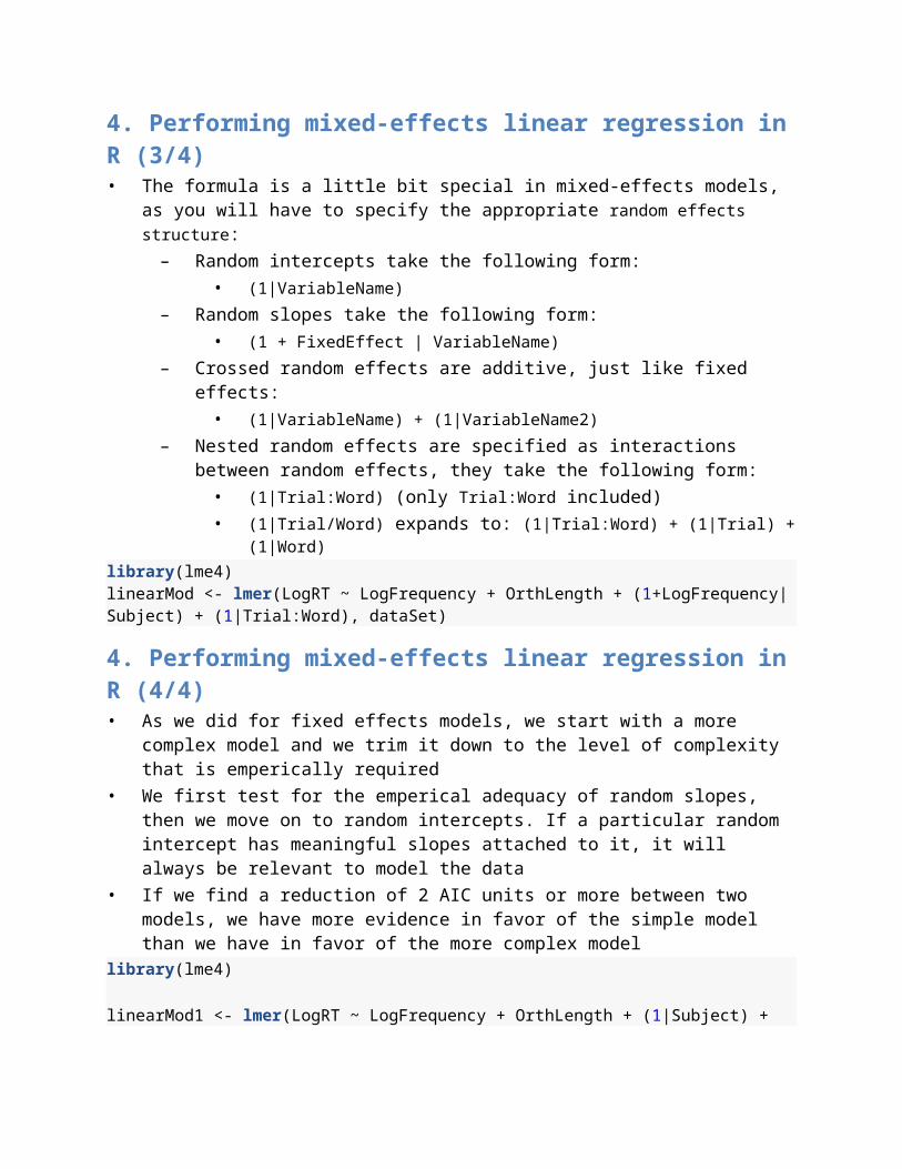
• (1|Trial:Word) (only Trial:Word included)• (1|Trial/Word) expands to: (1|Trial:Word) + (1|Trial) + (1|

Word)library(lme4)linearMod <- lmer(LogRT ~ LogFrequency + OrthLength + (1+LogFrequency|Subject) + (1|Trial:Word), dataSet)

4. Performing mixed-effects linear regression in R (4/4)• As we did for fixed effects models, we start with a more complex model and we trim it

down to the level of complexity that is emperically required• We first test for the emperical adequacy of random slopes, then we move on to

random intercepts. If a particular random intercept has meaningful slopes attached to it, it will always be relevant to model the data

• If we find a reduction of 2 AIC units or more between two models, we have more evidence in favor of the simple model than we have in favor of the more complex model

library(lme4)

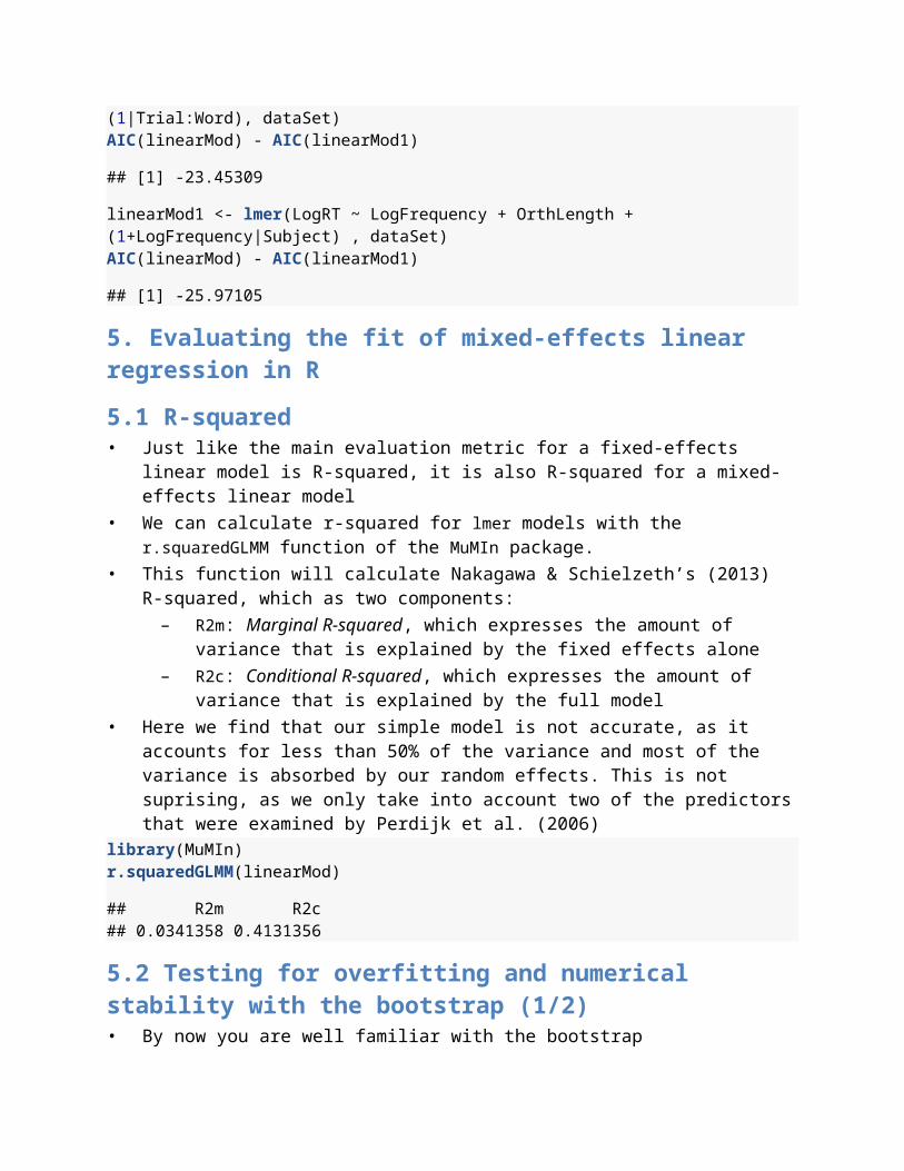
linearMod1 <- lmer(LogRT ~ LogFrequency + OrthLength + (1|Subject) + (1|Trial:Word), dataSet)AIC(linearMod) - AIC(linearMod1)

## [1] -23.45309

linearMod1 <- lmer(LogRT ~ LogFrequency + OrthLength + (1+LogFrequency|Subject) , dataSet)AIC(linearMod) - AIC(linearMod1)

## [1] -25.97105

5. Evaluating the fit of mixed-effects linear regression in R

5.1 R-squared• Just like the main evaluation metric for a fixed-effects linear model is R-squared, it is

also R-squared for a mixed-effects linear model• We can calculate r-squared for lmer models with the r.squaredGLMM function of the

MuMIn package.• This function will calculate Nakagawa & Schielzeth’s (2013) R-squared, which as two

components:– R2m: Marginal R-squared, which expresses the amount of variance that is

explained by the fixed effects alone– R2c: Conditional R-squared, which expresses the amount of variance that is

explained by the full model

• Here we find that our simple model is not accurate, as it accounts for less than 50% of the variance and most of the variance is absorbed by our random effects. This is not suprising, as we only take into account two of the predictors that were examined by Perdijk et al. (2006)

library(MuMIn)r.squaredGLMM(linearMod)

## R2m R2c ## 0.0341358 0.4131356

5.2 Testing for overfitting and numerical stability with the bootstrap (1/2)• By now you are well familiar with the bootstrap• The lme4 package has a build-in function to generate bootstrap confidence intervals

with the percentile method• Bootstrapping is a so-called ‘embarrassingly parallel’ problem, so we can generate a

considerable speed increase by using parallel computing:– Windows users should set the parallel argument to snow– Mac users should set the parallel argument to multicore– ncpus should be set to the amount of CPU cores your computer has. Typically 4

for a recent laptop, 2 for older laptopsintervals <- confint(linearMod, method="boot", boot.type="perc", nsim=1000, parallel="multicore", ncpus=4)

5.2 Testing for overfitting and numerical stability with the bootstrap (2/2)• The interpretation is the same as always, with some extras:

– The rows that are named .sig01 etc. refer to the random effects, in the same order as they appear on the summary. The confidence region is for the standard deviation of the intercepts and for the pairwise correlation coefficients between the random effects (if you have random slopes)

– The row that is named .sigma refers to the residual. The confidence region is for the standard deviation

– Wide confidence intervals point to numerical instability and/or overfitting– Confidence intervals that include zero point to numerical instability and/or

overfitting

6. Interpreting mixed-effects linear models

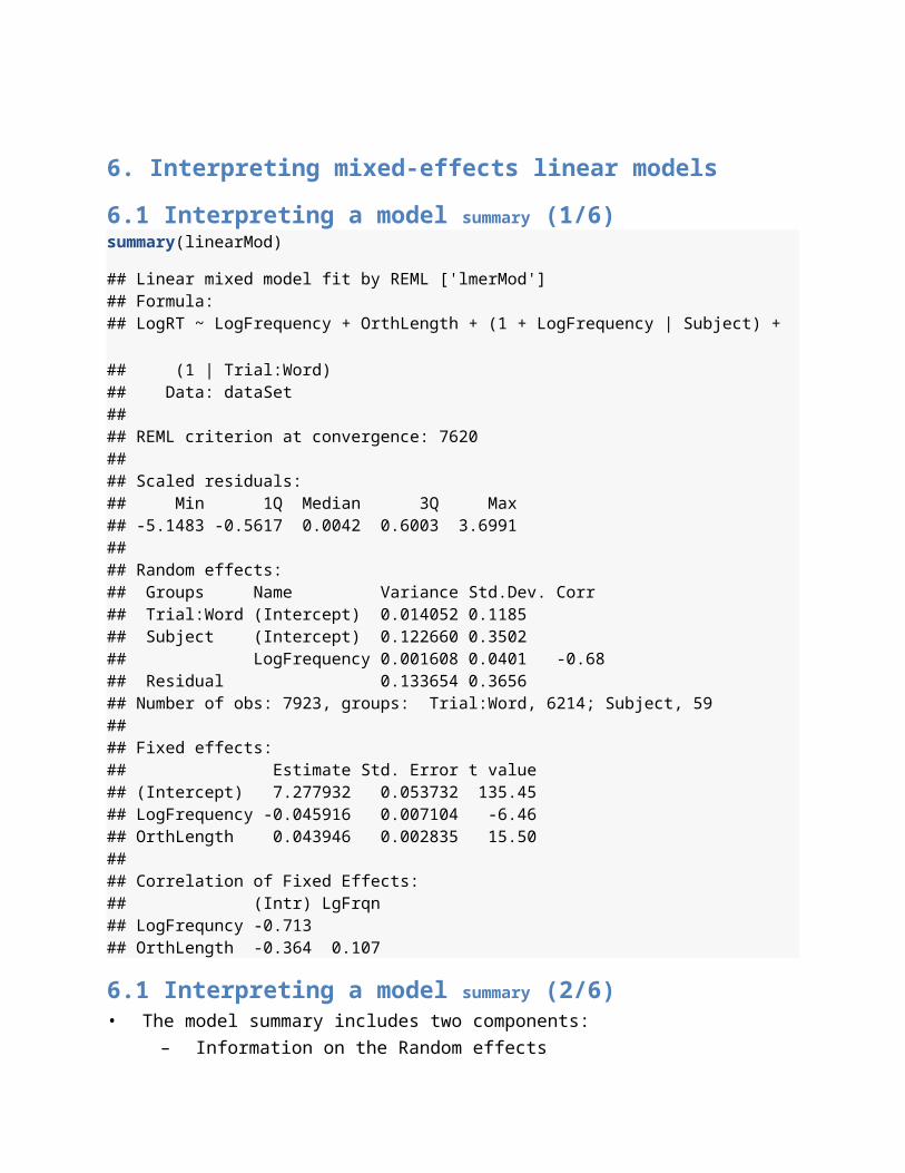
6.1 Interpreting a model summary (1/6)summary(linearMod)

## Linear mixed model fit by REML ['lmerMod']## Formula: ## LogRT ~ LogFrequency + OrthLength + (1 + LogFrequency | Subject) +

## (1 | Trial:Word)## Data: dataSet## ## REML criterion at convergence: 7620## ## Scaled residuals: ## Min 1Q Median 3Q Max ## -5.1483 -0.5617 0.0042 0.6003 3.6991 ## ## Random effects:## Groups Name Variance Std.Dev. Corr ## Trial:Word (Intercept) 0.014052 0.1185 ## Subject (Intercept) 0.122660 0.3502 ## LogFrequency 0.001608 0.0401 -0.68## Residual 0.133654 0.3656 ## Number of obs: 7923, groups: Trial:Word, 6214; Subject, 59## ## Fixed effects:## Estimate Std. Error t value## (Intercept) 7.277932 0.053732 135.45## LogFrequency -0.045916 0.007104 -6.46## OrthLength 0.043946 0.002835 15.50## ## Correlation of Fixed Effects:## (Intr) LgFrqn## LogFrequncy -0.713 ## OrthLength -0.364 0.107

6.1 Interpreting a model summary (2/6)• The model summary includes two components:

– Information on the Random effects– Information on the fixed effects

6.1 Interpreting a model summary (3/6)• Random effects:

– Variance: Variance estimate of the intercepts. Larger variances point to more dispersion in the intercept values

– Std.Dev.: Standard deviation of the intercepts. Larger standard deviations point to more dispersion in the intercept values. If you obtain a low standard deviation and variance estimate, this is an indication that the random intercept may be superfluous

– LogFrequency: Standard deviation and variance of the slope estimates for the different subjects

– Corr: If the model includes random slopes, the summary includes a correlation estimate for the slope and the intercept.

• If you have multiple random slopes attached to the same random intercept, the first correlation coefficient describes the relationship of the slope and the intercept, the following describe the relationships between the random slopes attached to the same intercept

• The value +/-1 should raise suspicion, as it is usually an indication of overparametrization (i.e., that you do not have enough data to evaluate the slope) (Baayen et al., 2008)

– Number of obs: Number of observations. The number of groups that follow allow you to compare the parameters-to-observations ratio. You can have a large number of random effects, but you will usually run into overfitting if you have a random effect for each individual observation

6.1 Interpreting a model summary (4/6)• Fixed effects:

– The interpretation of the fixed effects in a lmer model is identical to the interpretation of the fixed effects in a lm model

– Estimate: Effect size estimates, on the same scale as the dependent variable– Std. Error: Standard error for the effect size estimate. Larger standard

errors point to less certainty regarding the effect size estimate– t-value: t-statistic, which allows us to gauge the certainty associated with

the effect size estimate

6.1 Interpreting a model summary (5/6)• You will have noticed that the output does not contain p-values• This is due to the fact that, in order to go from the t-statistic to a precise p-value, you

need to be able to estimate the degrees of freedom accurately.• At the moment, no agreed upon method exists for estimating the degrees of freedom

implied by the random effects of a linear mixed-effects model: does a random effect with 400 levels counts as 1 degree of freedom or rather as 400? (Bates, 2006; Baayen et al., 2008)

6.1 Interpreting a model summary (6/6)• This means that we have to interpret the t-statistic in an approximate way, which may

be too conservative:– As per a standard t-table, with two degrees of freedom we can accept a result to

be significant in a two-tailed test with alpha = 0.05 when the t-value is more extreme than +/-4.303

– Most of our models will have more degrees of freedom, so if we accept as statistically significant at p < 0.05 t-values more extreme than +/-4.303, we are well in the clear

– For really large datasets (N > 10,000) we could even lower this threshold to t=2 (Baayen et al., 2008: 398, note 1)

• If a reviewer ever demands you to produce p-values, fake a smile, say “thank you” and refer to Baayen et al. (2008) and Bates (2006).

• The lmer function from the lmerTest package will produce precise p-values, but these have been shown to be unreliable in some cases (Li & Redden, 2015)

6.2 Interpreting Random Effects: Individual variation in language processing and production (1/3)• Most studies that use mixed-effects models will approach random effects as control

variables: covariates you include in the model to compensate for potential idiosyncrasies in your data

• If you are interested in the behavior of individuals vs. the overall trend at the level of the speech community, random effects contain a wealth of information, as they allow you to investigate how individuals diverge from the speech community trend (see e.g., Claes, 2016: Chap. 9; Drager & Hay, 2012; Forrest, 2015 for examples)

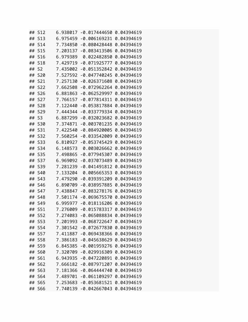
6.2 Interpreting Random Effects: Individual variation in language processing and production (2/3)• You can inspect the coefficients attached to a random variable with coef(model)

$VariableName:– By comparing the (Intercept) column to the intercept we obtain from

summary(linearModel) of the model, we can see how much faster or slower specific subjects respond in comparison to the population mean

– LogFrequency has a by-subject random slope. The coefficients we get for this variable are adjusted for speaker’s increased or decreased sensitivity to frequency.

coef(linearMod)$Subject

## (Intercept) LogFrequency OrthLength## S10 7.296312 -0.053615369 0.04394619## S12 6.938017 -0.017444650 0.04394619## S13 6.975459 -0.006169231 0.04394619## S14 7.734850 -0.080428448 0.04394619## S15 7.203137 -0.083413506 0.04394619

## S16 6.979389 0.022482850 0.04394619## S18 7.429719 -0.071925777 0.04394619## S2 7.435002 -0.051352842 0.04394619## S20 7.527592 -0.047740245 0.04394619## S21 7.257130 -0.026371608 0.04394619## S22 7.662508 -0.072962264 0.04394619## S26 6.881863 -0.062529997 0.04394619## S27 7.766157 -0.077814311 0.04394619## S28 7.122440 -0.053817884 0.04394619## S29 7.444344 -0.033779334 0.04394619## S3 6.887299 -0.032023682 0.04394619## S30 7.374871 -0.003701235 0.04394619## S31 7.422540 -0.084920005 0.04394619## S32 7.560254 -0.033542009 0.04394619## S33 6.810927 -0.053745429 0.04394619## S34 6.148573 0.003026662 0.04394619## S35 7.498865 -0.077945307 0.04394619## S37 6.969092 -0.037073489 0.04394619## S39 7.281239 -0.041491812 0.04394619## S40 7.133204 0.005665353 0.04394619## S43 7.479290 -0.039391209 0.04394619## S46 6.890709 -0.038957885 0.04394619## S47 7.438847 -0.083278176 0.04394619## S48 7.501174 -0.069675570 0.04394619## S49 6.995977 -0.018116206 0.04394619## S51 7.276009 -0.015783317 0.04394619## S52 7.274083 -0.065088834 0.04394619## S53 7.201993 -0.068722647 0.04394619## S54 7.301542 -0.072677830 0.04394619## S57 7.411887 -0.069438366 0.04394619## S58 7.386183 -0.045638629 0.04394619## S59 6.845385 -0.001959276 0.04394619## S60 7.320709 -0.029916309 0.04394619## S61 6.943935 -0.047220891 0.04394619## S62 7.666182 -0.087971207 0.04394619## S63 7.181366 -0.064444740 0.04394619## S64 7.489701 -0.061109297 0.04394619## S65 7.253683 -0.053681521 0.04394619## S66 7.740139 -0.042667043 0.04394619## S67 7.369915 -0.048840537 0.04394619## S68 7.448463 -0.059707719 0.04394619## S69 6.880806 -0.026889241 0.04394619## S7 7.741079 -0.080356099 0.04394619## S70 6.919119 0.010020270 0.04394619## S71 7.568417 -0.046036666 0.04394619## S72 7.517811 -0.062409759 0.04394619## S73 7.404212 -0.041811441 0.04394619## S74 7.133311 -0.052415383 0.04394619## S75 6.821473 -0.002080022 0.04394619## S76 6.596212 0.050816656 0.04394619

## S77 7.498175 -0.084126668 0.04394619## S78 7.510114 -0.072041751 0.04394619## S79 7.793184 -0.061340539 0.04394619## S8 7.856130 -0.083424236 0.04394619

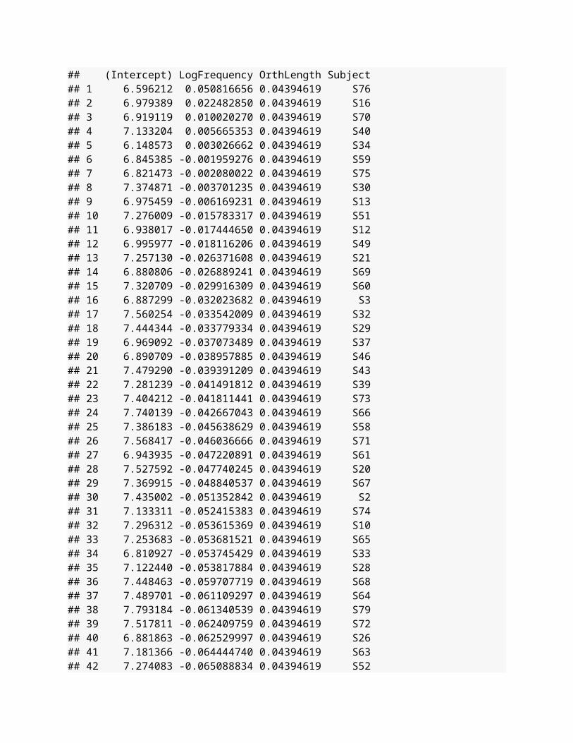
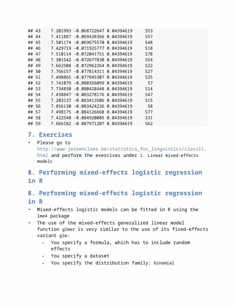
6.2 Interpreting Random Effects: Individual variation in language processing and production (3/3)• Since the coefficients table is a data.frame we can use the dplyr function arrange

to sort the table by order of LogFrequency• The function desc sorts in descending order• This will erase the rownames, so we need to store the Subject IDs in a variable first by

assigning rownames(subjects) to a new column• Sorting the estimates allows us to see that there is a sizeable difference between

subjects when it comes to their reaction to LogFrequency:– For some speakers, there is a positive effect, whereas for most speakers, the

effect is negative– For speakers who are inherently faster (lower intercept values), LogFrequency

tends to have a smaller negative or even a positive effectlibrary(dplyr)subjects<- coef(linearMod)$Subject subjects %>% mutate(Subject=rownames(subjects)) %>% arrange(desc(LogFrequency))

## (Intercept) LogFrequency OrthLength Subject## 1 6.596212 0.050816656 0.04394619 S76## 2 6.979389 0.022482850 0.04394619 S16## 3 6.919119 0.010020270 0.04394619 S70## 4 7.133204 0.005665353 0.04394619 S40## 5 6.148573 0.003026662 0.04394619 S34## 6 6.845385 -0.001959276 0.04394619 S59## 7 6.821473 -0.002080022 0.04394619 S75## 8 7.374871 -0.003701235 0.04394619 S30## 9 6.975459 -0.006169231 0.04394619 S13## 10 7.276009 -0.015783317 0.04394619 S51## 11 6.938017 -0.017444650 0.04394619 S12## 12 6.995977 -0.018116206 0.04394619 S49## 13 7.257130 -0.026371608 0.04394619 S21## 14 6.880806 -0.026889241 0.04394619 S69## 15 7.320709 -0.029916309 0.04394619 S60## 16 6.887299 -0.032023682 0.04394619 S3## 17 7.560254 -0.033542009 0.04394619 S32## 18 7.444344 -0.033779334 0.04394619 S29## 19 6.969092 -0.037073489 0.04394619 S37## 20 6.890709 -0.038957885 0.04394619 S46## 21 7.479290 -0.039391209 0.04394619 S43## 22 7.281239 -0.041491812 0.04394619 S39

## 23 7.404212 -0.041811441 0.04394619 S73## 24 7.740139 -0.042667043 0.04394619 S66## 25 7.386183 -0.045638629 0.04394619 S58## 26 7.568417 -0.046036666 0.04394619 S71## 27 6.943935 -0.047220891 0.04394619 S61## 28 7.527592 -0.047740245 0.04394619 S20## 29 7.369915 -0.048840537 0.04394619 S67## 30 7.435002 -0.051352842 0.04394619 S2## 31 7.133311 -0.052415383 0.04394619 S74## 32 7.296312 -0.053615369 0.04394619 S10## 33 7.253683 -0.053681521 0.04394619 S65## 34 6.810927 -0.053745429 0.04394619 S33## 35 7.122440 -0.053817884 0.04394619 S28## 36 7.448463 -0.059707719 0.04394619 S68## 37 7.489701 -0.061109297 0.04394619 S64## 38 7.793184 -0.061340539 0.04394619 S79## 39 7.517811 -0.062409759 0.04394619 S72## 40 6.881863 -0.062529997 0.04394619 S26## 41 7.181366 -0.064444740 0.04394619 S63## 42 7.274083 -0.065088834 0.04394619 S52## 43 7.201993 -0.068722647 0.04394619 S53## 44 7.411887 -0.069438366 0.04394619 S57## 45 7.501174 -0.069675570 0.04394619 S48## 46 7.429719 -0.071925777 0.04394619 S18## 47 7.510114 -0.072041751 0.04394619 S78## 48 7.301542 -0.072677830 0.04394619 S54## 49 7.662508 -0.072962264 0.04394619 S22## 50 7.766157 -0.077814311 0.04394619 S27## 51 7.498865 -0.077945307 0.04394619 S35## 52 7.741079 -0.080356099 0.04394619 S7## 53 7.734850 -0.080428448 0.04394619 S14## 54 7.438847 -0.083278176 0.04394619 S47## 55 7.203137 -0.083413506 0.04394619 S15## 56 7.856130 -0.083424236 0.04394619 S8## 57 7.498175 -0.084126668 0.04394619 S77## 58 7.422540 -0.084920005 0.04394619 S31## 59 7.666182 -0.087971207 0.04394619 S62

7. Exercises• Please go to http://www.jeroenclaes.be/statistics_for_linguistics/class11.html and

perform the exercises under 1. Linear mixed-effects models

8. Performing mixed-effects logistic regression in R

8. Performing mixed-effects logistic regression in R• Mixed-effects logistic models can be fitted in R using the lme4 package• The use of the mixed-effects generalized linear model function glmer is very similar to

the use of its fixed-effects variant glm:

– You specify a formula, which has to include random effects– You specify a dataset– You specify the distribution family: binomial

• For corpus-linguistic research, it is best to specify the bobyqa optimizer function (a function that does some very technical stuff behind the scenes) rather than the default optimizer

glmer(dependent ~ predictor1 + predictor2 + (1|random), family="binomial", control=glmerControl(optimizer="bobyqa"))

8. Performing mixed-effects logistic regression in R: data• In this class we will be working with the dataset analyzed in Claes(2014, 2016):

– In standard Spanish, the NP of existential haber is a direct object, for which the verb normally does not agree with plural NPs. In many varieties of Spanish, variable agreement can be found

– The data records the following characteristics:• Type: Singular or plural haber• Typical.Action.Chain.Pos: Typical role the referent of the noun

fulfills in events: Heads (entities that are likely to start an action) vs. Tails-Settings (entities that are likely to suffer an action or constitute the setting in which an action takes place)

• Tense: preterit and present vs. all others• Pr.2.Pr: The type of haber clause that was last used by the speaker, up

until a 20-clause lag• Co.2.Pr: The type of haber clause that was last used by the interviewer,

up until a 20-clause lag• Polarity: negation absent vs present• Style: data collection method (interview, reading task, questionnaire

task)• Gender: gender• Age: 21-35 years vs. 55+ years• Education: University vs. less• Noun: lemma of the head noun of the NP• Speaker: Speaker ID

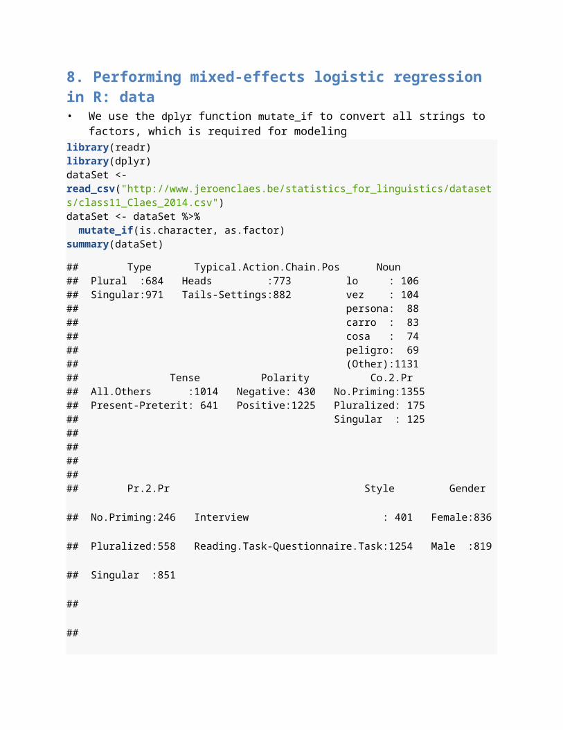
8. Performing mixed-effects logistic regression in R: data• We use the dplyr function mutate_if to convert all strings to factors, which is

required for modelinglibrary(readr)library(dplyr)dataSet <- read_csv("http://www.jeroenclaes.be/statistics_for_linguistics/datasets/class11_Claes_2014.csv")dataSet <- dataSet %>%

mutate_if(is.character, as.factor)summary(dataSet)

## Type Typical.Action.Chain.Pos Noun ## Plural :684 Heads :773 lo : 106 ## Singular:971 Tails-Settings:882 vez : 104 ## persona: 88 ## carro : 83 ## cosa : 74 ## peligro: 69 ## (Other):1131 ## Tense Polarity Co.2.Pr ## All.Others :1014 Negative: 430 No.Priming:1355 ## Present-Preterit: 641 Positive:1225 Pluralized: 175 ## Singular : 125 ## ## ## ## ## Pr.2.Pr Style Gender

## No.Priming:246 Interview : 401 Female:836

## Pluralized:558 Reading.Task-Questionnaire.Task:1254 Male :819

## Singular :851

##

##

##

##

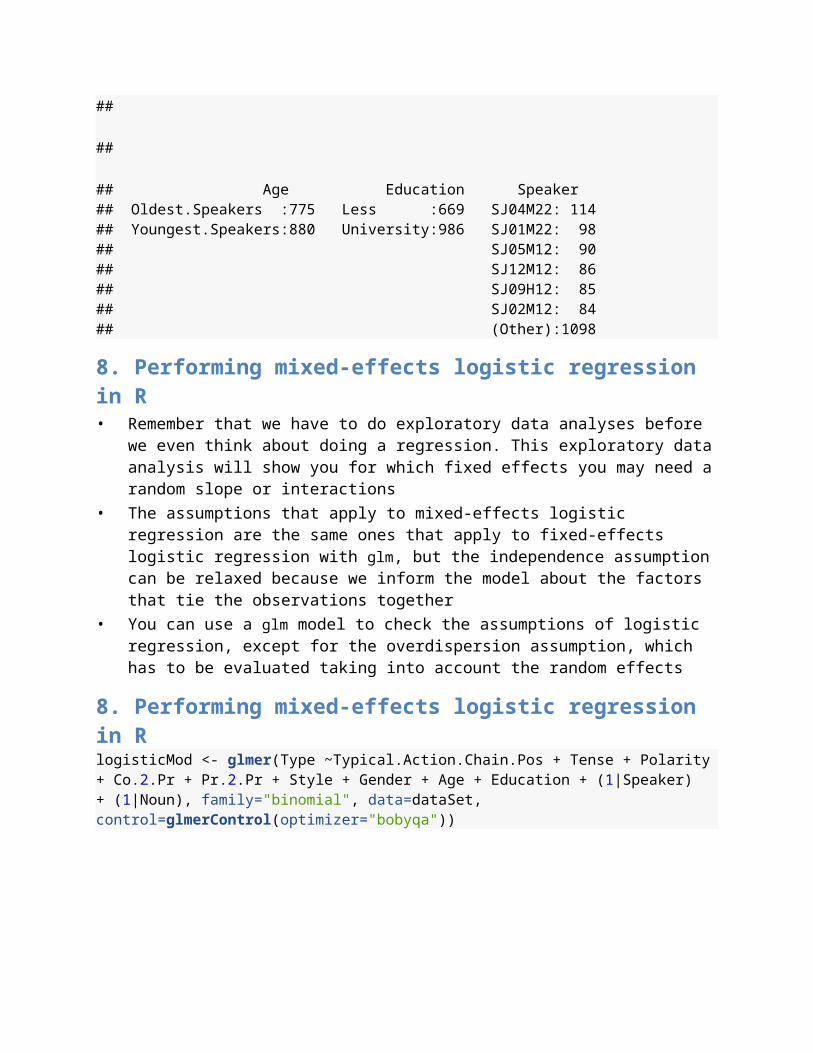
## Age Education Speaker ## Oldest.Speakers :775 Less :669 SJ04M22: 114 ## Youngest.Speakers:880 University:986 SJ01M22: 98 ## SJ05M12: 90 ## SJ12M12: 86 ## SJ09H12: 85 ## SJ02M12: 84 ## (Other):1098

8. Performing mixed-effects logistic regression in R• Remember that we have to do exploratory data analyses before we even think about

doing a regression. This exploratory data analysis will show you for which fixed effects you may need a random slope or interactions

• The assumptions that apply to mixed-effects logistic regression are the same ones that apply to fixed-effects logistic regression with glm, but the independence assumption can be relaxed because we inform the model about the factors that tie the observations together

• You can use a glm model to check the assumptions of logistic regression, except for the overdispersion assumption, which has to be evaluated taking into account the random effects

8. Performing mixed-effects logistic regression in RlogisticMod <- glmer(Type ~Typical.Action.Chain.Pos + Tense + Polarity + Co.2.Pr + Pr.2.Pr + Style + Gender + Age + Education + (1|Speaker) + (1|Noun), family="binomial", data=dataSet, control=glmerControl(optimizer="bobyqa"))

9. Assessing the fit of mixed-effects logistic regression in R

9. Assessing the fit of mixed-effects logistic regression in R (1/3)• To assess the fit of linear regression models, we used R-squared. However, this

measure is not as straighforwardly interpreted in logistic regression as it is in linear regression, where it represents the amount of variance explained

• We can calculate a pseudo-R-squared for glmer models with the r.squaredGLMM function of the MuMIn package.

• This function will calculate Nakagawa & Schielzeth’s (2013) pseudo-R-squared.• Values above 0.50 are indicative of a good fit, as the pseudo-R-squared hardly reaches

the high levels true R-squared reaches in linear regression• As was the case for the mixed-effects linear model, the model returns a marginal and a

conditional estimate.library(MuMIn)r.squaredGLMM(logisticMod)

## R2m R2c ## 0.4804269 0.5594299

9. Assessing the fit of mixed-effects logistic regression in R (2/3)• To assess the discriminative power of logistic regression models,the C-index of

concordance is commonly used (also know as Area under Reciever Operating Characteristic Curve; AUROC), which can be calculated with the somers2 function of the Hmisc package

• The C-index expresses how good the model is at classifying the observations in the two classes. In particular, it expresses the probability that the model will predict the second class in cases where the second class is observed (Harrell, 2015: 257)

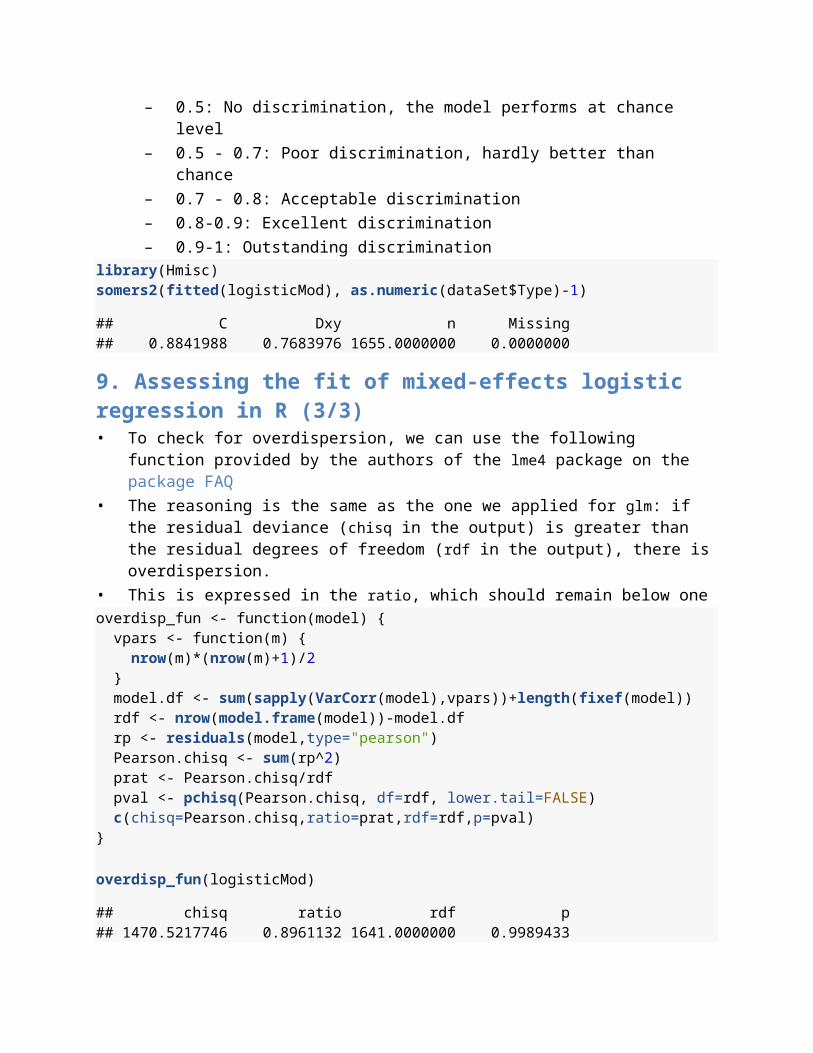
• Hosmer et al. (2013: 177) propose the following classification of C-index values:– 0.5: No discrimination, the model performs at chance level– 0.5 - 0.7: Poor discrimination, hardly better than chance– 0.7 - 0.8: Acceptable discrimination

– 0.8-0.9: Excellent discrimination– 0.9-1: Outstanding discrimination

library(Hmisc)somers2(fitted(logisticMod), as.numeric(dataSet$Type)-1)

## C Dxy n Missing ## 0.8841988 0.7683976 1655.0000000 0.0000000

9. Assessing the fit of mixed-effects logistic regression in R (3/3)• To check for overdispersion, we can use the following function provided by the

authors of the lme4 package on the package FAQ• The reasoning is the same as the one we applied for glm: if the residual deviance

(chisq in the output) is greater than the residual degrees of freedom (rdf in the output), there is overdispersion.

• This is expressed in the ratio, which should remain below oneoverdisp_fun <- function(model) { vpars <- function(m) { nrow(m)*(nrow(m)+1)/2 } model.df <- sum(sapply(VarCorr(model),vpars))+length(fixef(model)) rdf <- nrow(model.frame(model))-model.df rp <- residuals(model,type="pearson") Pearson.chisq <- sum(rp^2) prat <- Pearson.chisq/rdf pval <- pchisq(Pearson.chisq, df=rdf, lower.tail=FALSE) c(chisq=Pearson.chisq,ratio=prat,rdf=rdf,p=pval)}

overdisp_fun(logisticMod)

## chisq ratio rdf p ## 1470.5217746 0.8961132 1641.0000000 0.9989433

10. Interpreting mixed-effects logistic regression

10. Interpreting mixed-effects logistic regression (1/4)summary(logisticMod)

## Generalized linear mixed model fit by maximum likelihood (Laplace## Approximation) [glmerMod]## Family: binomial ( logit )## Formula: Type ~ Typical.Action.Chain.Pos + Tense + Polarity + Co.2.Pr + ## Pr.2.Pr + Style + Gender + Age + Education + (1 | Speaker) + ## (1 | Noun)## Data: dataSet## Control: glmerControl(optimizer = "bobyqa")##

## AIC BIC logLik deviance df.resid ## 1544.2 1620.0 -758.1 1516.2 1641 ## ## Scaled residuals: ## Min 1Q Median 3Q Max ## -9.7218 -0.5353 0.1724 0.4698 3.8881 ## ## Random effects:## Groups Name Variance Std.Dev.## Noun (Intercept) 0.3785 0.6152 ## Speaker (Intercept) 0.2114 0.4598 ## Number of obs: 1655, groups: Noun, 169; Speaker, 24## ## Fixed effects:## Estimate Std. Error z value## (Intercept) -1.1737 0.4226 -2.778## Typical.Action.Chain.PosTails-Settings 0.7694 0.2049 3.755## TensePresent-Preterit 3.1982 0.2097 15.253## PolarityPositive -0.6409 0.1940 -3.304## Co.2.PrPluralized -0.5207 0.3191 -1.632## Co.2.PrSingular 0.1972 0.3477 0.567## Pr.2.PrPluralized -0.8194 0.2441 -3.356## Pr.2.PrSingular 0.2415 0.2370 1.019## StyleReading.Task-Questionnaire.Task 0.2430 0.2831 0.858## GenderMale 0.5167 0.2361 2.189## AgeYoungest.Speakers -0.2996 0.2371 -1.264## EducationUniversity 0.8362 0.2395 3.492## Pr(>|z|) ## (Intercept) 0.005476 ** ## Typical.Action.Chain.PosTails-Settings 0.000174 ***## TensePresent-Preterit < 2e-16 ***## PolarityPositive 0.000954 ***## Co.2.PrPluralized 0.102687 ## Co.2.PrSingular 0.570645 ## Pr.2.PrPluralized 0.000790 ***## Pr.2.PrSingular 0.308158 ## StyleReading.Task-Questionnaire.Task 0.390756 ## GenderMale 0.028611 * ## AgeYoungest.Speakers 0.206208 ## EducationUniversity 0.000480 ***## ---## Signif. codes: 0 '***' 0.001 '**' 0.01 '*' 0.05 '.' 0.1 ' ' 1## ## Correlation of Fixed Effects:## (Intr) T.A.C. TnsP-P PlrtyP C.2.PP C.2.PS P.2.PP P.2.PS SR.T-Q## Ty.A.C.PT-S -0.331

## TnsPrsnt-Pr -0.321 0.228

## PolartyPstv -0.408 0.017 0.025

## C.2.PrPlrlz -0.358 -0.023 0.021 0.014

## C.2.PrSnglr -0.229 -0.079 -0.048 -0.041 0.379

## Pr.2.PrPlrl -0.220 -0.021 -0.001 -0.033 -0.118 -0.038

## Pr.2.PrSngl -0.206 0.014 0.000 -0.048 -0.124 -0.083 0.795

## StylR.T-Q.T -0.447 0.100 0.156 0.129 0.605 0.380 -0.330 -0.355

## GenderMale -0.314 -0.020 0.077 -0.025 0.014 0.028 0.011 -0.017 0.037## AgYngst.Spk -0.250 -0.017 -0.036 0.018 -0.021 -0.003 -0.010 -0.004 -0.085## EdctnUnvrst -0.329 0.021 0.113 0.003 0.007 0.031 -0.005 -0.041 -0.020## GndrMl AgYn.S## Ty.A.C.PT-S ## TnsPrsnt-Pr ## PolartyPstv ## C.2.PrPlrlz ## C.2.PrSnglr ## Pr.2.PrPlrl ## Pr.2.PrSngl ## StylR.T-Q.T ## GenderMale ## AgYngst.Spk 0.000 ## EdctnUnvrst 0.062 0.017

10. Interpreting mixed-effects logistic regression (2/4)• Random effects:

– Variance: Variance estimate of the intercepts. Larger variances point to more dispersion in the intercept values

– Std.Dev.: Standard deviation of the intercepts. Larger standard deviations point to more dispersion in the intercept values. If you obtain a low standard deviation and variance estimate, this is an indication that the random intercept may be superfluous

– If your model includes random slopes, you also get the standard deviation and variance of the slope estimates

– Corr: If the model includes random slopes, the summary includes a correlation estimate for the slope and the intercept.

• If you have multiple random slopes attached to the same random intercept, the first correlation coefficient describes the relationship of the slope and the intercept, the following describe the relationships between the random slopes attached to the same intercept

• The value +/-1 should raise suspicion, as it is usually an indication of overparametrization (i.e., that you do not have enough data to evaluate the slope) (Baayen et al., 2008)

– Number of obs: Number of observations. The number of groups that follow allow you to compare the parameters-to-observations ratio. You can have a large number of random effects, but you will usually run into overfitting if you have a random effect for each individual observation

10. Interpreting mixed-effects logistic regression (3/4)• Fixed effects:

– The interpretation of the fixed effects in a mixed-effects model is the same as in a glm model

– Estimate: Effect size estimates, on the Log Odds (logit) scale– Std. Error: Standard error for the effect size estimate. Larger standard

errors point to less certainty regarding the effect size estimate– z value: z-statistic, which allows us to gauge the certainty associated with

the effect size estimate– Pr(>|z|): In a logistic model, the estimation of the degrees of freedom is less

problematic, so we do get p-values for our effect estimates

10. Interpreting mixed-effects logistic regression (4/4)• Recall that we should apply Occam’s razor to our models before settling down on a

model! You can do this by removing one fixed/random effect at a time and comparing the AIC values of models

11. Testing for overfitting and numerical stability with the bootstrap

11. Testing for overfitting and numerical stability with the bootstrap (1/2)• The lme4 package has a build-in function to generate bootstrap confidence intervals

with the percentile method. This function works in the same way for glmer as for lmer

• Bootstrapping is a so-called ‘embarrassingly parallel’ problem, so we can generate a considerable speed increase by using parallel computing:

– Windows users should set the parallel argument to snow– Mac users should set the parallel argument to multicore– ncpus should be set to the amount of CPU cores your computer has. Typically 4

for a recent laptop, 2 for older laptopsintervals <- confint(logisticMod, method="boot", boot.type="perc", nsim=1000, parallel="multicore", ncpus=4)

11. Testing for overfitting and numerical stability with the bootstrap (2/2)• The interpretation is the same as always, with some extras:

– The rows that are named .sig01 etc. refer to the random effects, in the same order as they appear on the summary. The confidence region is for the standard deviation of the intercepts and for the pairwise correlation coefficients between the random effects (if you have random slopes)

– The row that is named .sigma refers to the residual. The confidence region is for the standard deviation of the slope estimates

– Wide confidence intervals (> 1 Log Odds) point to numerical instability and/or overfitting

– Confidence intervals that include zero point to numerical instability and/or overfitting

• Here we find that Age, and Style have wide confidence regions, which is rather unsurprising given their lack of significance. We should remove these effects from our analysis

.sig01

.sig02

(Intercept)

Typical.Action.Chain.PosTails-Settings

TensePresent-Preterit

PolarityPositive

Co.2.PrPluralized

Co.2.PrSingular

Pr.2.PrPluralized

Pr.2.PrSingular

StyleReading.Task-Questionnaire.Task

GenderMale

AgeYoungest.Speakers

EducationUniversity

12. Reporting on mixed-effects models• You should clearly state all of your data transformation steps and describe your

exploratory analysis• You should clearly explain how you have searched for the appropriate random effects

structure:– First you have searched for random effects using exploratory data analysis

– Then you have trimmed down the random effects using AIC comparisons and single-term deletions

• You should clearly explain how you have searched for interactions• You report the Estimates, Standard Errors, T/Z-values and, for glmer, the p-values of

the fixed effects• You report the standard deviation and variance for the random effects; for random

slopes you also report the correlation coefficient• As for summary statistics, you report:

– AIC– deviance– R-squared– For logistic models, you also report the c-index of concordance

13. Exercises• Please go to http://www.jeroenclaes.be/statistics_for_linguistics/class11.html and

perform the exercises under 2. Logistic mixed-effects models

14. References• Baayen, R. H. (2013). languageR: Data sets and functions with “Analyzing Linguistic

Data: A practical introduction to statistics”. https://cran.r-project.org/web/packages/languageR/index.html.

• Baayen, R. H., Davidson, D. J., Bates, D. M. (2008). Mixed-effects modeling with crossed random effects for subjects and items. Journal of Memory and Language 59(4). 392-412.

• Barr, D. J., Levy, R., Scheepers, C., & Tily, H. J. (2013). Random effects structure for confirmatory hypothesis testing: Keep it maximal. Journal of Memory and Language 68(3). 255-278.

• Bates, D. M. (2006). lmer, p-values and all that. Message send to the R-help mailing list, May 19, 2006. https://stat.ethz.ch/pipermail/r-help/2006-May/094765.html. Consulted May 3, 2018.

• Bates, D., Kliegl, R., Vasishth, S., & Baayen, R. H. (2015). Parsimonious mixed models. Available from: arXiv:1506.04967.

• Claes, J. (2014). A Cognitive Construction Grammar approach to the pluralization of presentational haber in Puerto Rican Spanish. Language Variation and Change 26(2). 219-246.

• Claes, J. (2016). Cognitive, social, and individual constraints on linguistic variation: A case study of presentational haber pluralization in Caribbean Spanish. Berlin/Boston, MA: De Gruyter.

• Drager, K., & Hay, J. (2012). Exploiting random intercepts: Two case studies in sociophonetics. Language Variation and Change 24(1). 59-78.

14. References• Forrest, J. (2015). Community rules and speaker behavior: Individual adherence to

group constraints on (ING). Language Variation and Change 27(3).377-406.• Harrell, F. (2015). Regression modeling strategies: With applications to linear models,

logistic regression, and survival analysis. New York, NY: Springer.• Hosmer, D., Lemeshow, S., Sturdivant, R. (2013). Applied logistic regression. Oxford:

Wiley.• Li, P., & Redden, D. T. (2015). Comparing denominator degrees of freedom

approximations for the generalized linear mixed model in analyzing binary outcome in small sample cluster-randomized trials. BMC Medical Research Methodology 15. Article 38.

• Matuschek, H., Kliegl, R., Vasishth, S., Baayen, R. H., & Bates, D. M. (2017). Balancing Type I error and power in linear mixed models. Journal of Memory and Language, 94(2). 305-315.

• Nakagawa, S, Schielzeth, H. (2013). A general and simple method for obtaining R² from Generalized Linear Mixed-effects Models. Methods in Ecology and Evolution 4. 133–142.

• Perdijk, K., Schreuder, R., Verhoeven, L. and Baayen, R. H. (2006) Tracing individual differences in reading skills of young children with linear mixed-effects models. Manuscript, Radboud University Nijmegen.

• Zuur, A. F., Leno, E. N., & Elphick, C. S. (2010). A protocol for data exploration to avoid common statistical problems. Methods in Ecology and Evolution 1(1). 3-14.