Topic 1: Introduction Sociology 6Z03 McMaster University€¦ · · 2016-09-14Sociology 6Z03 Topic 1: Introduction John Fox McMaster University Fall 2016 John Fox (McMaster University)

Sociology 6Z03Topic 1: Introduction

John Fox

McMaster University

Fall 2016

John Fox (McMaster University) Sociology 6Z03Topic 1: Introduction Fall 2016 1 / 31

Outline

Why study statistics?

Lying with statistics.

Statistical data.


Why Study Statistics?

“Thou shalt not sit with statisticians nor commit a social science.”– W. H. Auden (1907-1973)



Thought Question

Who was W. H. Auden?

A The founding professor of the Department of Sociology at McMaster University.

B A famous poet.

C An early hip-hop artist.

D A prime minister of Canada.

E I don’t know.



Auden notwithstanding, a great deal of interesting and important work in sociology —and in other social sciences, not to mention medical, biological, and natural sciences, andthe popular media — employs statistical methods.

This will be partly demonstrated by the illustrations that I employ during the course ofthe semester and in the illustrations in the text, and partly by your work in other courses.


Why Study Statistics?The Challenger Disaster: Bad Statistical Analysis Can Kill You

The Challenger disaster (from Edward Tufte’s book, Visual Explanations, Cheshire CT:Graphics Press, 1997). Sometimes poor statistical data analysis is costly:

On January 28, 1986, the U. S. space shuttle Challenger exploded shortly after blastoff,killing seven astronauts. See <http://en.wikipedia.org/wiki/File:

Challenger_-_STS-51-L_Explosion.ogg>.


http://en.wikipedia.org/wiki/File:Challenger_-_STS-51-L_Explosion.ogg

http://en.wikipedia.org/wiki/File:Challenger_-_STS-51-L_Explosion.ogg


The cause of the explosion was the failure of rubberO-rings sealing two sections of one of the booster rocketsattached to the shuttle (B and C in the cross-sectionpicture to the right).

This failure, in turn, was caused by the low temperature atthe time of launch which made the O-rings lose theirelasticity.



On the day before the ill-fated launch, engineers at Morton Thiokol, the company thatbuilt the boosters, recommended that the launch be postponed because of the lowforecast temperature for the following day.

Using a graph essentially similar to the one on the next slide, officials at NASA andThiokol examined data concerning O-ring damage that had occurred on previouslaunches; although some of these incidents were serious, none was disastrous.

These officials determined that there was no convincing evidence linking O-ring failure toambient temperature, and they decided to proceed with the launch.

Thus, the Challenger disaster took place even though its cause was identified on the daybefore the accident.



Index of extent of O-ring damage by temperature (degrees F) at time of launch, for shuttlelaunches prior to the Challenger disaster in which O-ring damage occurred. (Source: Adaptedfrom Tufte, Visual Explanations, page 45.)

Temperature (degrees Farenheit) of field joints at time of launch

O−

ring

dam

age

inde

x

●

● ●

●

●● ●

25 30 35 40 45 50 55 60 65 70 75 80 85

04

812

26−29 degree range of forcasted temperatures for the launch of space−shuttle Challenger on January 28, 1986



Thought Question

What does the graph show?

A The extent of O-ring damage is not related to temperature.

B There tends to be more O-ring damage at high temperatures than at low temperatures.

C There tends to be more O-ring damage at low temperatures than at high temperatures.

D The graph doesn’t have enough information to know whether O-ring damage is related totemperature.

E I don’t know.



The problem with the preceding graph is that it doesn’t include launches on which noO-ring damage occurred.

An effective presentation of the data makes the relationship between O-ring damage andtemperature clear.



Index of extent of O-ring damage by temperature (in degrees Farenheit) at time of launch, forall shuttle launches prior to the Challenger disaster. (Source: Redrawn and slightly adaptedfrom Tufte, Visual Explanations, page 45.)

Temperature (degrees Farenheit) of field joints at time of launch

O−

ring

dam

age

inde

x

●

● ●

●

●● ●

● ●●●

● ● ●●

● ● ● ●●

● ● ●

25 30 35 40 45 50 55 60 65 70 75 80 85

04

812

26−29 degree range of forcasted temperatures for the launch of space−shuttle Challenger on January 28, 1986

●

●

some damageno damage



Thought Question

What does the graph show?

A The extent of O-ring damage is not clearly related to temperature.

B There tends to be more O-ring damage at high temperatures than at low temperatures.

C There tends to be more O-ring damage at low temperatures than at high temperatures.

D The graph doesn’t have enough information to know whether O-ring damage is related totemperature.

E I don’t know.



To understand quantitative work in sociology (about half the field), as well as reports inthe popular media (e.g., on the results of polls and social surveys), it is important to havea basic knowledge of statistical methods.

Many occupations require individuals to produce and interpret statistical data, and toanalyze data, typically with the help of a computer. See, e.g.,<http://www.nytimes.com/2009/08/06/technology/06stats.html>.

Statistical reasoning has its own logic and fundamental concepts. It is interesting.

Methods of statistical data analysis and inference are among the most importantintellectual products of the last century.


http://www.nytimes.com/2009/08/06/technology/06stats.html

Lying With Statistics

“Lies, damned lies and statistics.” – attributed to Benjamin Disraeli (1804-1881)

There is a common conception that it is particularly simple to “prove whatever you wantto prove” using statistical data.

I believe that statistics lends itself no more to deception than other forms of argument, andindeed careful analysis of data makes self-deception — if not deception of others — moredifficult.In analyzing data, I am often struck by how hard it is to find what I expect to find, and howfrequently I discover characteristics of data that I did not anticipate. I find it much easier tofool myself when I evaluate non-quantitative evidence.

Fooling others is, however, another matter, but the modes of statistical deception areessentially the same as in any other misleading presentation of “evidence.”


Lying With StatisticsKinds of Lies

Outright lies: At one extreme, you can make up or falsify data.

Consider the following table, published by the British psychologist Sir Cyril Burt (1961), andpurporting to show the relationship between the average IQ scores of children and adults insix “social classes”:

Social ClassAdults’

Mean IQChildren’sMeanI Q

Higher Professional 139.7 120.8Lower Professional 130.6 114.7Clerical 115.9 107.8Skilled 108.2 104.6Semiskilled 97.8 98.9Unskilled 84.9 92.6



A graph of Burt’s “data” reveals the fraud:

90 100 110 120 130 140

9010

011

012

013

0

Adults' Mean IQ

Chi

ldre

n's

Mea

n IQ ●

●

●●

●

● Unskilled

Semiskilled

Skilled

Clerical

Lower Professional

Higher Professional



Thought Question

How can you tell from the graph that Burt’s data were “cooked”?

A We can’t tell that the data were falsified just by looking at the graph.

B It is well known that Cyril Burt committed scientific fraud.

C Real data wouldn’t line up perfectly along a straight line.

D I don’t know.



It is ironic that the quantitative character of the fraud facilitated its detection (see, e.g.,Kamin, The Science and Politics of I. Q., 1974), but one can make up data more cleverly.

Be skeptical when you evaluate a study (and not only of statistical results).The possibility of falsification of data is one of the reasons that replication of results isimportant in science.



Obfuscation: At another extreme, you can take advantage of the ignorance andinsecurity of your audience, overwhelming them with details and procedures that they donot understand.

It is especially confusing when different “experts” use the same data to support opposingconclusions.One shouldn’t expect magic from statistical studies: It is, for example, difficult to drawconvincing causal evidence from observational data.Be critical of the design of statistical (and other) studies.

Partial Truth: And, of course, you can present accurate information partially andselectively to support a conclusion that is not supported by a more complete analysis ofthe available evidence.

Be alert to apparent omissions in a presentation (again, not only of statistical evidence).When data are public, you can subject them to your own analysis


Statistical DataThe Data Table

Statistical data are usually organized as tables in which the rows of the table representunits of observation (such as individuals or countries) and the columns represent variablesor characteristics of the units (such as age, gender, and annual income for individuals, orarea, type of political system, and per-capita income for countries).

Part of an illustrative dataset is shown on the next slide.

The full dataset includes 207 nations. The information in this table was collected around1998.The data are ordered alphabetically, which is not terribly useful.As in many real datasets, some of the information in the data table is missing.



Nation GDP Per Capita, $US Infant Mortality per 1000 Region

Afghanistan 2,848 154 AsiaBosnia 271 13 EuropeCanada 18,943 6 AmericasChile 4,736 13 AmericasChina 582 38 AsiaCongo 1,008 90 AfricaCuba 1,983 9 AmericasGaza Strip missing 37 AfricaIsrael 16,738 7 AsiaLibya 5,498 56 AfricaUnited Kingdom 18,913 6 EuropeUnited States 26,037 7 Americas



Thought Question

In this data table:

A The units of observation are nations and the variables include GDP per capita (averagegross domenstic product per person, in US dollars), infant-mortality rate (number of infantdeaths per 1,000 live births), and region.

B The units of observation are GDP per capita, infant-mortality rate, and region, and thevariables are the nations.

C I don’t know.


Statistical Data

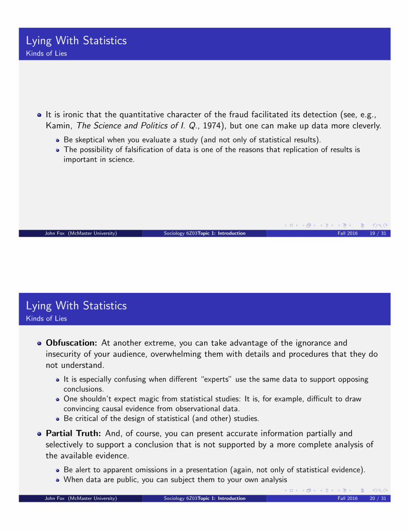
Here is a graph showing the relationship between infant mortality and GDP per capita, withdifferent symbols for the several regions of the world:

0 10000 20000 30000 40000

0

50

100

150

GDP per Capia (US Dollars)

Infa

nt M

orta

lity

Rat

e (p

er 1

000)

●

●

●

●

●

●

●

●

●

●

●

●●

●

●

●

●

●

●

●

●

●

●

●

●

●

●

●

●

●

●

●

●

●

●

●

●

●

●

●

●

●

●

●

●

●

●

●

●

●

●

●

●

●

●

Region

AfricaAmericaAsiaEuropeOceania

Afghanistan

French.Guiana

Gabon

Iraq

Liberia

Libya

Myanmar

Sierra.Leone

Switzerland



Thought Question

What does this graph show?

A As GDP per capita rises, infant mortality also tends to rise.

B As GDP per capita rises, infant mortality tends to decline.

C GDP per capita and infant mortality do not appear to be related.

D I don’t know.


Statistical DataKinds of Data

Two of the variables in the table — GDP per capita and infant-mortality — arequantitative; region, in contrast, is a qualitative, categorical variable.

There are several sorts of quantitative data:

Counts, such as the number of individuals residing in a country. Counts are non-negativeintegers (whole numbers).Amounts, such as GDP per capita. Amounts are also non-negative, but they need not beintegers.

Amounts are also called ratio variables, because it is meaningful to form ratios of two values(i.e., divide one value by another).As the table shows, for example, the per-capita GDP in Canada was US$18,943, while that inChile was $4,736. Thus, Canada had a per-capita GDP that was 18,943/4,736, or 4.0 times, aslarge as that of Chile.The unit of a ratio variable (e.g., the dollar) is arbitrary, but the zero point of the scale (zeroGDP per capita) is not.



Quantitative data (continued):

Relative Frequencies, including proportions, percents, and rates.

Proportions, percents, and many types of rates have both minimum and maximum values.The infant-mortality rate, for example, is defined as

1,000 × number of children dying in their first year

number of live births

and has a minimum of 0 and a maximum of 1,000.Some types of rates, however, can exceed 1,000. For example, the total fertility rate is definedas the average number of children born to a group of 1,000 women surviving through theirchild-bearing years, and typically takes on values well in excess of 1,000.



Quantitative data (continued):

Interval Scales, which have both an arbitrary unit of measurement and an arbitrary zero point.

A simple example is Celsius temperature, because 0 on the Celsius scale does not represent “noheat.”Here we can compare ratios of differences — intervals — of scale scores, but we cannot formratios of the scores themselves.Thus, the temperature difference between 10 and 20 degrees Celsius is the same as between 30and 40 degrees, but 40 is not twice as hot as 20.Some methods for constructing scales of attitudes, judgments, and abilities produce intervalscales.



There are two common types of categorical data:

Qualitative or nominal variables (such as region in the data table) in which there is nointrinsic order to the categories.Ordinal variables, in which the categories have a natural order.

For example, survey respondents are often asked about their degree of agreement with anattitude statement, recording their responses in several ordered categories, such as StronglyAgree, Agree, Neutral, Disagree, Strongly Disagree.



Thought Question

Consider the following two variables: (1) Gender (male and female) and (2) Education(in years).

A Both variables are quantitative variables.

B Both variables are categorical variables.

C Gender is a quantitative variable and education is a categorical variable.

D Gender is a categorical variable and education is a quantitative variable.

E I don’t know.



Important Point

The methods of analysis that are appropriate to statistical data are partly dependent upon thenature of the variables.

Different methods usually apply to qualitative variables, for example, than to quantitativevariables.


Documents

Topic 1: Introduction Sociology 6Z03 McMaster University€¦ · · 2016-09-14Sociology 6Z03 Topic 1: Introduction John Fox McMaster University Fall 2016 John Fox (McMaster University)