Topic 1:

Introduction(Mankiw chapter 1) updated 9/23/09

Intermediate Macroeconomic Theory

slide 2

Learning objectivesThis chapter introduces you to

• the issues macroeconomists study

• the tools macroeconomists use

• some important concepts in macroeconomic analysis

slide 3

Three main variables we will study:1) Gross domestic product, output (GDP)

2) Inflation in the cost of living (CPI)

3) Unemployment rate

We will begin by looking at trends in the data for these, and make initial observations.

slide 4

slide 5

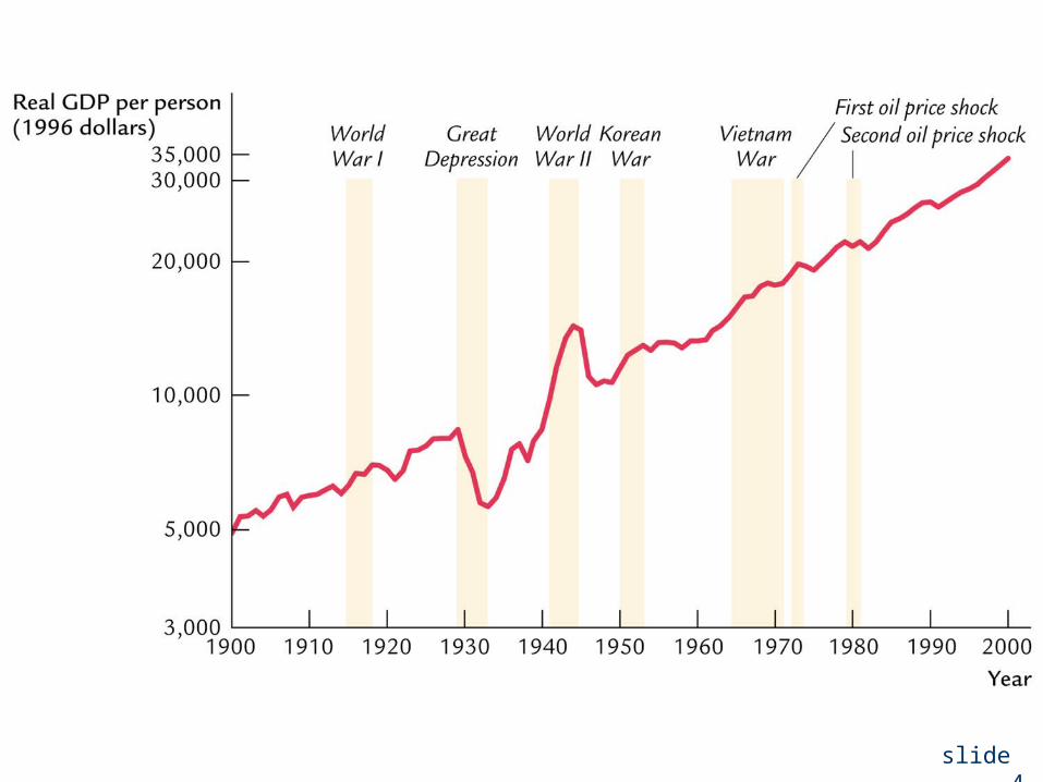
GDP: Observations1. Long-term upward trend. Income more

than doubled over last 30 years.2. Short-run disruptions in the trend:

recessions.

slide 6

slide 7

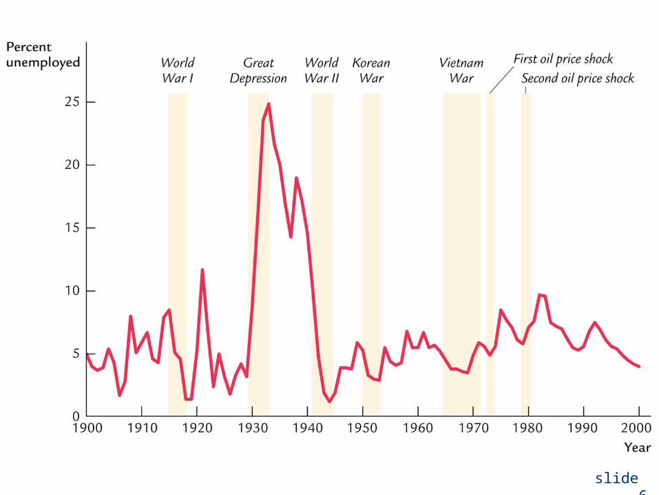
Unemployment: Observations1. Unemployment always positive.2. Fluctuations related to GDP:

unemployment higher during recessions.

slide 8

slide 9

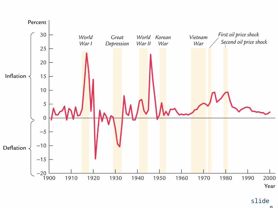
Inflation: Observations1. Inflation can be negative.2. Often high when GDP high, but not

always (see 1970s).

slide 10

How we learn Economics: Models…are simplied versions of a more complex reality

• irrelevant details are stripped away

Used to • show the relationships between economic

variables• explain the economy’s behavior• devise policies to improve economic

performance

slide 11

Example of a model: The supply & demand for new cars

• explains the factors that determine the price of cars and the quantity sold.

• assumes the market is competitive: each buyer and seller is too small to affect the market price

• Variables:Q

d = quantity of cars that buyers demandQ

s = quantity that producers supplyP = price of new carsY = aggregate income

slide 12

The demand for cars

shows that the quantity of cars consumers demand

is related to the price of cars and aggregate income.

demand equation: ( , )dQ D P Y

slide 13

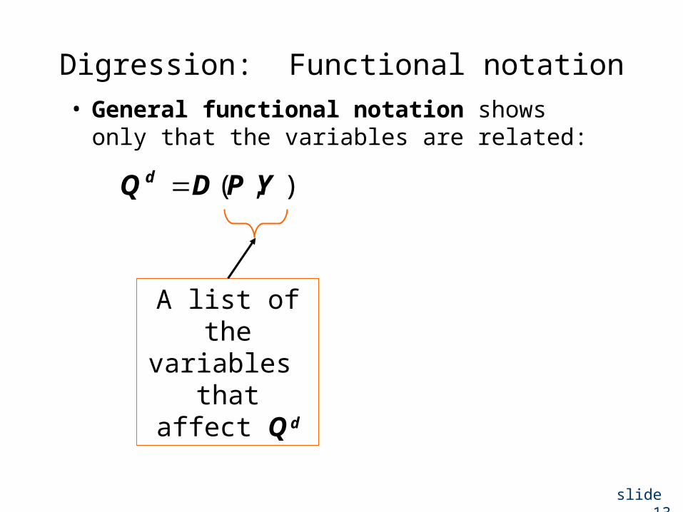
Digression: Functional notation• General functional notation shows only that

the variables are related:

( , )dQ D P Y

A list of the variables

that affect Q d

slide 14

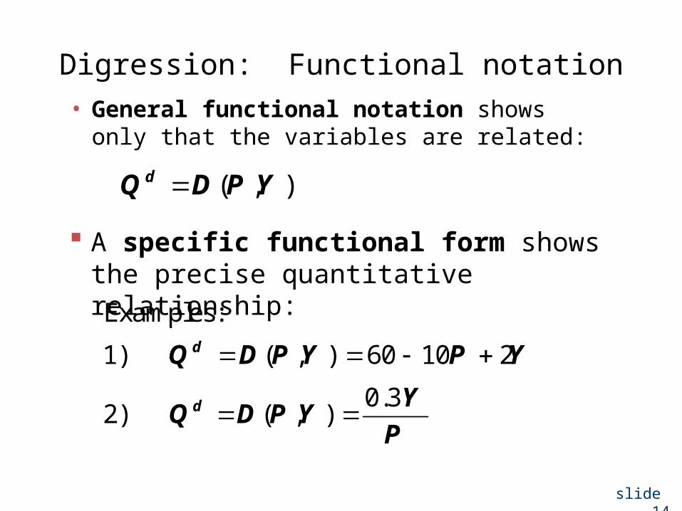
Digression: Functional notation• General functional notation shows only that

the variables are related:

( , )dQ D P Y

A specific functional form shows the precise quantitative relationship:

Examples:

1) ( , ) 60 10 2 dQ D P Y P Y

0.3

2) ( , )d YQ D P Y

P

slide 15

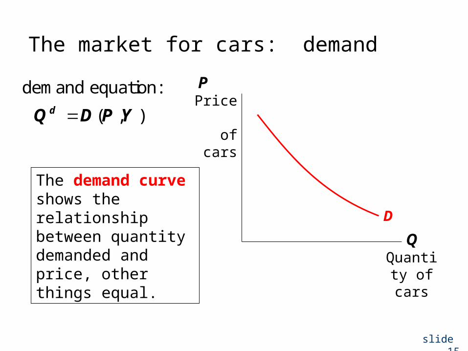
The market for cars: demand

Q Quantit

y of cars

P Price

of cars

D

The demand curve shows the relationship between quantity demanded and price, other things equal.

demand equation:

( , )dQ D P Y

slide 16

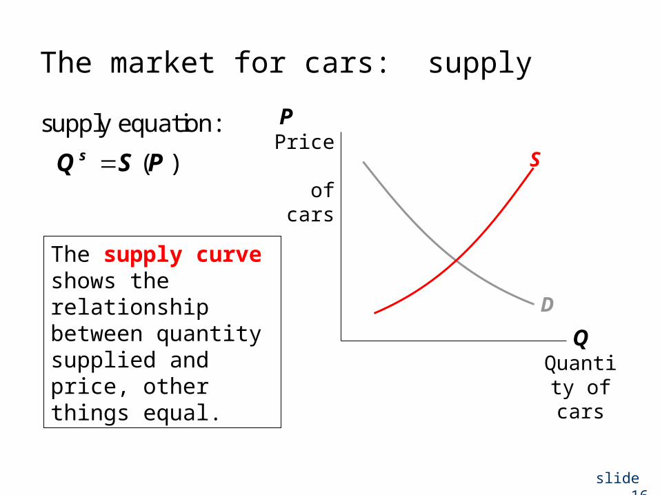
The market for cars: supply

Q Quantit

y of cars

P Price

of cars

D

supply equation:

( )sQ S P S

The supply curve shows the relationship between quantity supplied and price, other things equal.

slide 17

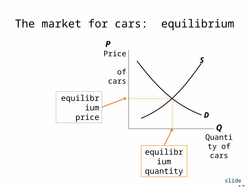
The market for cars: equilibrium

Q Quantit

y of cars

P Price

of cars S

D

equilibrium price

equilibriumquantity

slide 18

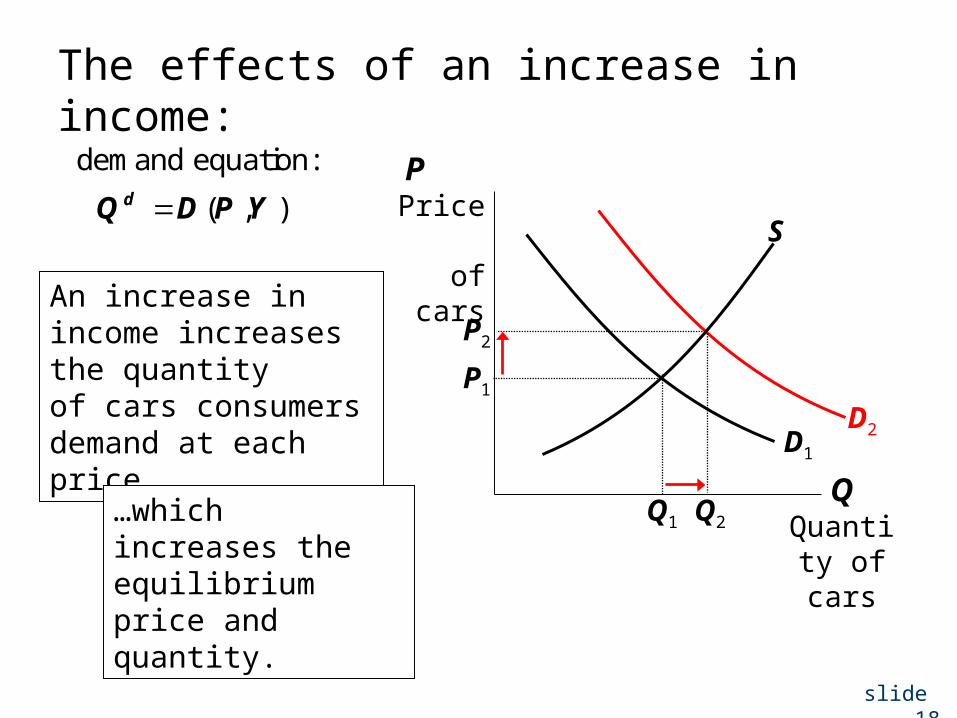
The effects of an increase in income:

D2

Q Quantit

y of cars

P Price

of cars S

D1

Q1

P1

An increase in income increases the quantity of cars consumers demand at each price…

…which increases the equilibrium price and quantity.

P2

Q2

demand equation:

( , )dQ D P Y

slide 19

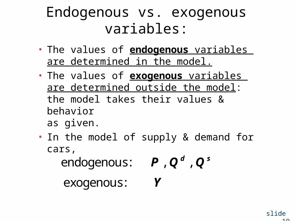
Endogenous vs. exogenous variables:

• The values of endogenous variables are determined in the model.

• The values of exogenous variables are determined outside the model: the model takes their values & behavior as given.

• In the model of supply & demand for cars,

endogenous: , , d sP Q Q

exogenous: Y

slide 20

A Multitude of ModelsNo one model can address all the issues we care about. For example,

If we want to know how a fall in aggregate income affects new car prices, we can use the S/D model for new cars.

But if we want to know why aggregate income falls, we need a different model.

slide 21

A Multitude of Models• So we will learn different models for studying

different issues (unemployment, inflation, growth).

• For each new model, you should keep track of – its assumptions, – which variables are endogenous and exogenous,– which questions it can help us understand,

slide 22

Prices: Flexible Versus Sticky• Market clearing: an assumption that prices are

flexible and adjust to equate supply and demand. • In the short run, many prices are sticky---they

adjust only sluggishly in response to supply/demand imbalances. For example,

– labor contracts that fix the nominal wage for a year or longer

– magazine prices that publishers change only once every 3-4 years

slide 23

Prices: Flexible Versus Sticky• The economy’s behavior depends partly on

whether prices are sticky or flexible:

• If prices are sticky, then demand won’t always equal supply. This helps explain– unemployment (excess supply of labor)– the occasional inability of firms to sell what they

produce

• Long run: prices flexible, markets clear, economy behaves very differently.

slide 24

Outline of the class:• Classical and Growth Theory (ch. 2-8)

How the economy works in the long run, when prices are flexible and markets work well.

• Business Cycle Theory (ch. 9-15)How the economy works in the short run, when prices are sticky. What can policy makers do when things go wrong.

• Microeconomic Foundations (Chaps. 16-17)Incorporate features from microeconomics on the behavior of consumers. (if time permits)