Top Tips from the DB2 Experts Blog - idug.org

1

Top Tips from the DB2 Experts Blog

Session: D01

Chris EatonIBM Toronto Lab

May 07, 2007 09:50 a.m. – 10:50 a.m.

Platform: DB2 LUW

AbstractChris Eaton writes what may be the most popular DB2 blog on the internet. With over 15,000 page views per month and over 250 unique visitors to his blog daily, "An Experts Guide to DB2 Technology" is helping people get their job done. Unlike typical blogs where the authors talk about what they ate for breakfast, Chris' blog is all about providing DB2 users with technical tips and sneak previews of upcoming technology. In this session, Chris will share his top 20 most popular DB2 tips from the postings on his blog over the last year. To get a preview, check it out at http://blogs.ittoolbox.com/database/technology/

2

2

Agenda• Introduction to My Blog• Tips on monitoring your database• Tips on storage management• Tips on efficient SQL• Tips on high availability• My favorite new features in DB2 9 from my blog

Outline:This course will cover the top 20 tips and techniques ranging from new features in DB2 9 to hints on storage management, performance tuning, monitoring your database and advanced diagnostics.

Objectives:Tips on monitoring your databaseTips on storage managementTips on efficient SQLTips on high availabilityMy favorite new features in DB2 9

3

3

What’s a blog?• BLOG comes from weB LOG• Like a journal or a diary• Authors write whatever they want whenever they

want and you can comment on what is written

• Often blogs are socially oriented – what I did yesterday, what I ate for breakfast, etc.

• My blog is all about tips on using DB2 for Linux, UNIX, Windows

Merriam-Webster Online Dictionary

Main Entry: blogPronunciation: 'blog’Function: nounEtymology: short for Weblog: a Web site that contains an online personal journal with reflections, comments, and often hyperlinks provided by the writer - blog·ger noun- blog·ging noun

4

4

My Blog• Hosted on ITtoolbox• Called “An Expert’s Guide to DB2 Technology”

• URL to main pagehttp://blogs.ittoolbox.com/database/technology

• Postings range from 1 to 3 per week• Focused on helping you use DB2 for Linux, UNIX, Windows• Gives you a preview of what’s coming in new releases

5

5

Sign up to get an email whenever I post

a new entry

Comments on blog entries show up here

Popular entries listed here

Latest entries in the center pane

Older postings in the archive

Here is a screen capture of the front page of my blog.

From here you can view recent and archived blog entries, comment on blog entries, see other peoples comments and my most popular entries. If you want to subscribe, you can enter your email address and you will be sent a notice any time I post a new blog entry.

6

6

Statistics about my blog• In 2006

• 180,800 page views (500 page views per day)• 230 unique visitors per day on average• 1100 subscribers

• 92 postings in 2006 in areas like:• What’s new in Viper (DB2 9)

• Partitioning, STMM, Compression, XML, etc• What’s new in 8.2.2• Monitoring your database with SQL• Powerful SQL (OLAP, recursive, select from insert)• and much more …

My blog has become more popular than I ever expected it would be.Makes me feel pressure to keep it updated :-)

7

7

Who is reading this blog?• I had no idea, so I asked people to send me an

email telling me what city they were reading from.• To date I have 194 cities spanning 42 countries

across 6 continents• Using Google maps I have plotted them all at

http://tinyurl.com/2anl6z

Go to the above link to see the current status of my blog community map. See if your city is represented.

8

8

Is your state, city represented?• Missing US states

• Alaska• Hawaii• Idaho• Kansas• Maine• Mississippi• Montana• Nevada

• New Mexico• North Dakota• Rhode Island• South Carolina• South Dakota• Vermont• West Virginia• Wyoming

Here is a screen capture of my blog map that I discussed on the previous slide. This shows just North America and the places people are viewing my blog from. If you go to the URL mentioned on the previous slide you can click on any of these pins to view the city names. You can also zoom in and convert to satellite image (and you may even be able to see your house from space ☺

9

9


10

10

SQL to View Notification Log • Show me all the Critical and Error messages in the last 24 hours

SELECT TIMESTAMP, SUBSTR(MSG,1,400) AS MSG FROM SYSIBMADM.PDLOGMSGS_LAST24HOURSWHERE MSGSEVERITY IN ('C','E') ORDER BY TIMESTAMP DESC

• Show me all the messages in the notify log from the last 3 days

SELECT TIMESTAMP, SUBSTR(MSG,1,400) AS MSGFROM TABLE

( PD_GET_LOG_MSGS( CURRENT TIMESTAMP - 3 DAYS) ) AS PD

ORDER BY TIMESTAMP DESC

There is an administrative view called SYSIBMADM.PDLOGMSGS_LAST24HOURS. This view shows you the messages that exist in the notification log over the last 24 hours. The DDL for this view is as follows:TIMESTAMPTIMEZONEINSTANCENAMEDBPARTITIONNUMDBNAMEPIDPROCESSNAMETIDAPPL_IDCOMPONENTFUNCTIONPROBEMSGNUMMSGTYPEMSGSEVERITYMSG

If you want to view notification log messages that are older then 24 hours then use the PD_GET_LOG_MSGS table function and specify the start time you want to view messages from. The columns returned from the table function are the same as those of the PDLOGMSGS_LAST24HOURS view.

11

11

SQL to View Database History • Show the average and maximum time taken to perform full backups

SELECT AVG(TIMESTAMPDIFF(4,CHAR(TIMESTAMP(END_TIME) - TIMESTAMP(START_TIME)))) AS AVG_BTIME,

MAX(TIMESTAMPDIFF(4,CHAR(TIMESTAMP(END_TIME) - TIMESTAMP(START_TIME)))) AS MAX_BTIME

FROM SYSIBMADM.DB_HISTORYWHERE OPERATION = 'B'

AND OPERATIONTYPE = 'F'

• Show any commands in the recovery history file that failed

SELECT START_TIME, SQLCODE, SUBSTR(CMD_TEXT,1,50)FROM SYSIBMADM.DB_HISTORY

WHERE SQLCODE < 0

The view SYSIBMADM.DB_HISTORY gives you SQL access to the contents of the recovery history file. You no longer need to run LIST HISTORY commands and parse the output. Instead you can run SQL scripts to look for exactly what you need from the recovery history file. The columns in this view that I think are important are (for all columns see the link below)DBPARTITIONNUM SMALLINT Database partition number.START_TIME VARCHAR(14) Timestamp marking the start of a logged event.END_TIME VARCHAR(14) Timestamp marking the end of a logged event.FIRSTLOG VARCHAR(254) Name of the earliest transaction log associated with an event.LASTLOG VARCHAR(254) Name of the latest transaction log associated with an event.BACKUP_ID VARCHAR(24) Backup identifier or unique table identifier.TABSCHEMA VARCHAR(128) Table schema.TABNAME VARCHAR(128) Table name.CMD_TEXT CLOB(2 M) Data definition language associated with a logged event.NUM_TBSPS INTEGER Number of table spaces associated with a logged event.TBSPNAMES CLOB(5 M) Names of the table spaces associated with a logged event.OPERATION CHAR(1) Operation identifier. See Table 332 for possible values.OPERATIONTYPE CHAR(1) Action identifier for an operation. See Table 332 for possible values.OBJECTTYPE CHAR(1) Identifier for the target object of an operation. The possible values are: D for full database, P for table space, and T for table.LOCATION VARCHAR(255) Full path name for files, such as backup images or load input file, that are associated with logged events.DEVICETYPE CHAR(1) Identifier for the device type associated with a logged event. This field determines how the LOCATION field is interpreted. The possible values are: A for TSM, C for client, D for disk, K for diskette, L for local, N (generated internally by DB2), O for other (for other vendor device support), P for pipe, Q for cursor, R for remote fetch data, S for server, T for tape, U for user exit, and X for X/Open XBSA interface.SQLCODE INTEGER SQL return code, as it appears in the SQLCODE field of the SQLCA.SQLSTATE VARCHAR(5) A return code that indicates the outcome of the most recently executed SQL statement, as it appears in the SQLSTATE field of the SQLCA.

Operation values and their associated types can be found herehttp://publib.boulder.ibm.com/infocenter/db2luw/v9/topic/com.ibm.db2.udb.admin.doc/doc/r0022351.htm

12

12

SQL to View Long Running Queries • Show the longest running SQL Statements currently executing in the database, along with

the authid of the person running the query ordered by elapsed time

SELECT ELAPSED_TIME_MIN,SUBSTR(AUTHID,1,10) AS AUTH_ID, AGENT_ID,APPL_STATUS,SUBSTR(STMT_TEXT,1,20) AS SQL_TEXT

FROM SYSIBMADM.LONG_RUNNING_SQLWHERE ELAPSED_TIME_MIN > 0ORDER BY ELAPSED_TIME_MIN DESC

ELAPSED_TIME_MIN AUTH_ID AGENT_ID APPL_STATUS SQL_TEXT---------------- -------- -------- ------------ --------------

6 EATON 878 LOCKWAIT update org set deptn

A very easy to use administrative view is the SYSIBMADM.LONG_RUNNING_SQL view which can quickly show you the longest running SQL statements currently executing in your database. The columns of interest are below

Column name Data type Description or corresponding monitor elementSNAPSHOT_TIMESTAMP TIMESTAMP Time the report was generated.ELAPSED_TIME_MIN INTEGER Elapsed time of the statement in minutes.AGENT_ID BIGINT Application Handle (agent ID)APPL_NAME VARRHAR(256) Application NameAPPL_STATUS VARCHAR(22) Application Status. AUTHID VARCHAR(128) Authorization IDINBOUND_COMM_ADDRESS VARCHAR(32) Inbound Communication AddressSTMT_TEXT CLOB(16 M) SQL Dynamic Statement TextDBPARTITIONNUM SMALLINT The database partition from which the data was retrieved for this row.

13

13

SQL to View Locks • Show the holder and the waiter of any application that is currently waiting on a lock

SELECT SMALLINT(AGENT_ID) AS WAITING_ID,SUBSTR(APPL_NAME, 1,10) AS WAITING_APP,SUBSTR(AUTHID,1,10) AS WAITING_USER,SMALLINT(AGENT_ID_HOLDING_LK) AS HOLDER_ID,LOCK_MODE AS HELD, LOCK_OBJECT_TYPE AS TYPE, LOCK_MODE_REQUESTED AS REQUEST

FROM SYSIBMADM.LOCKWAITS

• Find the holding application, the userid (and client hostname) and the status of the lock holder

SELECT SUBSTR(APPL_NAME, 1,10) AS HOLDING_APP,SUBSTR(PRIMARY_AUTH_ID,1,10) AS HOLDING_USER,SUBSTR(CLIENT_NNAME,1,20) AS HOLDING_CLIENT,APPL_STATUS

FROM SYSIBMADM.SNAPAPPL_INFOWHERE AGENT_ID = 831

The first statement above shows you who is waiting on locks and who is holding the locks that others are waiting on. This information comes from the SYSIBMADM.LOCKWAITS view. If you want to drill down on the holding application, you can get more details out of the SYSIBMADM.SNAPAPPL_INFO view as shown in the second query. Of course you can simply join the two views into a single query but I’ll leave that as an exercise for the student.

Here are the column definitions for the LOCKWAITS view (object types and object modes are fully described herehttp://publib.boulder.ibm.com/infocenter/db2luw/v9/topic/com.ibm.db2.udb.admin.doc/doc/r0022018.htm )Column name Data type Description or corresponding monitor elementSNAPSHOT_TIMESTAMP TIMESTAMP Date and time the report was generated.DB_NAME VARCHAR(128) db_name - Database Name monitor elementAGENT_ID BIGINT Application Handle (agent ID) monitor elementAPPL_NAME VARCHAR(256) Application Name monitor elementAUTHID VARCHAR(128) Authorization ID monitor elementTBSP_NAME VARCHAR(128) tTable Space Name monitor elementTABSCHEMA VARCHAR(128) Table Schema Name monitor elementTABNAME VARCHAR(128) Table Name monitor elementSUBSECTION_NUMBER BIGINT Subsection Number monitor elementLOCK_OBJECT_TYPE VARCHAR(18) Lock Object Type Waited On monitor element. LOCK_WAIT_START_TIME TIMESTAMP Lock Wait Start Timestamp monitor elementLOCK_NAME VARCHAR(32) Lock Name monitor elementLOCK_MODE VARCHAR(10) Lock Mode monitor element. LOCK_MODE_REQUESTED VARCHAR(10) Lock Mode Requested monitor element. AGENT_ID_HOLDING_LK BIGINT Agent ID Holding Lock monitor elementAPPL_ID_HOLDING_LK VARCHAR(128) Application ID Holding Lock monitor elementLOCK_ESCALATION SMALLINT Lock Escalation monitor elementDBPARTITIONNUM SMALLINT

14

14

SQL to View Useful Table Information• A very useful view to see table information like the size of parts of the table (index, table,

xml data)

SELECT SUBSTR(TABSCHEMA,1,10) AS SCHEMA, SUBSTR(TABNAME,1,15) AS TABNAME,INT(DATA_OBJECT_P_SIZE) AS OBJ_SZ_KB, INT(INDEX_OBJECT_P_SIZE) AS INX_SZ_KB,INT(XML_OBJECT_P_SIZE) AS XML_SZ_KB

FROM SYSIBMADM.ADMINTABINFOWHERE TABSCHEMA='EATON'ORDER BY 3 DESC

• Or you can look at the total size of your tables by schema (or by tablespace)

SELECT SUBSTR(TABSCHEMA,1,10) AS SCHEMA, SUM(DATA_OBJECT_P_SIZE) AS OBJ_SZ_KB, SUM(INDEX_OBJECT_P_SIZE) AS INX_SZ_KB, SUM(XML_OBJECT_P_SIZE) AS XML_SZ_KB

FROM SYSIBMADM.ADMINTABINFOGROUP BY TABSCHEMAORDER BY 2 DESC

This is one of my favorite new views in DB2 9. Now I can see many of the related objects for a table and see their sizes with one simple query. For example the first query shows me the size of table data, index data and any XML data for each table in the EATON schema ordered by data size descending. The second query shows me the total size of all the objects for each of my schemas. You can also use this view to see if tables are in any inconsistent states and you can see the dictionary size for compressed tables and/or if the table is using large rids.

Here is the column definitions for this view:TABSCHEMA VARCHAR(128) Schema name.TABNAME VARCHAR(128) Table name.TABTYPE CHAR(1) Table type:DBPARTITIONNUM SMALLINT Database partition number.DATA_PARTITION_ID INTEGER Data partition number.AVAILABLE CHAR(1) State of the tableDATA_OBJECT_L_SIZE BIGINT Data object logical size. DATA_OBJECT_P_SIZE BIGINT Data object physical size. INDEX_OBJECT_L_SIZE BIGINT Index object logical size. INDEX_OBJECT_P_SIZE BIGINT Index object physical size. LONG_OBJECT_L_SIZE BIGINT Long object logical size. LONG_OBJECT_P_SIZE BIGINT Long object physical size. LOB_OBJECT_L_SIZE BIGINT LOB object logical size. LOB_OBJECT_P_SIZE BIGINT LOB object physical size. XML_OBJECT_L_SIZE BIGINT XML object logical size. XML_OBJECT_P_SIZE BIGINT XML object physical size. INDEX_TYPE SMALLINT Indicates the type of indexes currently in use for the table. REORG_PENDING CHAR(1) 'Y' indicates a reorg recommended alter has been applied and a classic (offline) reorg is required.INPLACE_REORG_STATUS VARCHAR(10) Current status of an inplace table reorganization. LOAD_STATUS VARCHAR(12) Current status of a load operation against the table. READ_ACCESS_ONLY CHAR(1) 'Y' if the table is in Read Access Only state. NO_LOAD_RESTART CHAR(1) 'Y' indicates the table is in a partially loaded state.NUM_REORG_REC_ALTERS SMALLINT Number of reorg recommend alter operations INDEXES_REQUIRE_ REBUILD CHAR(1) 'Y' if any of the indexes on the table require a rebuild. LARGE_RIDS CHAR(1) Indicates whether or not the table is using large row IDs (RIDs)LARGE_SLOTS CHAR(1) Indicates whether or not the table is using large slots DICTIONARY_SIZE BIGINT Size of the dictionary, in bytes, used for row compression if a row compression dictionary

15

15

SQL to View Registry Variables • Now you no longer need to log on to the server and run a command line

db2set command to display the value of your registry variables

• Here is an example that shows the value of the registry variableDB2_WORKLOAD

SELECT SUBSTR(REG_VAR_NAME,1,20) AS NAME, DBPARTITIONNUM, SUBSTR(REG_VAR_VALUE,1,20) AS VALUE

FROM SYSIBMADM.REG_VARIABLESWHERE REG_VAR_NAME = 'DB2_WORKLOAD'

Using this new REG_VARIABLES administrative view, you can view (but you cannot update) any of the registry variables that are set on a given server. Simply connect to any database on that server and query this view to see the names and values of any registry variable.

The contents of this view are as follows:DBPARTITIONNUM SMALLINT Logical partition number of each database partition on which thefunction operates.REG_VAR_NAME VARCHAR(256) Name of the DB2 registry variable.REG_VAR_VALUE VARCHAR(2048) Current setting of the DB2 registry variable.IS_AGGREGATE SMALLINT Indicates whether or not the DB2 registry variable is an aggregate variable.AGGREGATE_NAME VARCHAR(256) Name of the aggregate if the DB2 registry variable is currently obtaining its value from a configured aggregate. LEVEL CHAR(1) Indicates the level at which the DB2 registry variable acquires its value.

16

16

SQL to View Top Dynamic SQL• Show the most executed dynamic SQL statement

SELECT SUBSTR(STMT_TEXT,1,50), NUM_EXECUTIONSFROM SYSIBMADM.TOP_DYNAMIC_SQLORDER BY NUM_EXECUTIONS DESCFETCH FIRST ROW ONLY

• Show the dynamic SQL statement that has the longest average execution time

SELECT SUBSTR(STMT_TEXT,1,50), AVERAGE_EXECUTION_TIME_SFROM SYSIBMADM.TOP_DYNAMIC_SQLORDER BY AVERAGE_EXECUTION_TIME_S DESCFETCH FIRST ROW ONLY

This can be one of your most critical new views to reference. It shows you the most important dynamic SQL statements, how many times they are being executed, average execution times, number of sorts per statement. You can use this view as a basis for tuning long running or most frequently executed queries.

The content of the view is:SNAPSHOT_TIMESTAMP TIMESTAMP Timestamp for the report.NUM_EXECUTIONS BIGINT Statement Compilations monitor elementAVERAGE_EXECUTION_TIME_S BIGINT Average execution time.STMT_SORTS BIGINT Statement Sorts monitor elementSORTS_PER_EXECUTION BIGINT Number of sorts per statement execution.STMT_TEXT CLOB(2 M) SQL Dynamic Statement Text monitor elementDBPARTITIONNUM SMALLINT The database partition from which the data was retrieved for this row.

17

17

Finding the Log Hog• Display information about the application that currently has the oldest

uncommitted unit of work open

SELECT AI.APPL_STATUS, SUBSTR(AI.PRIMARY_AUTH_ID,1,10) AS "Authid",SUBSTR(AI.APPL_NAME,1,15) AS "Appl Name",INT(AP.UOW_LOG_SPACE_USED/1024/1024)

AS "Log Used (M)", INT(AP.APPL_IDLE_TIME/60) AS "Idle for (min)", AP.APPL_CON_TIME AS "Connected Since"

FROM SYSIBMADM.SNAPDB DB, SYSIBMADM.SNAPAPPL AP,SYSIBMADM.SNAPAPPL_INFO AI

WHERE AI.AGENT_ID = DB.APPL_ID_OLDEST_XACT AND AI.AGENT_ID = AP.AGENT_ID;

In this example we are looking for the information about the application that is currently the oldest transaction that is holding up the log tail. This transaction represents the total amount of recovery log that must now be scanned in order to perform crash recover. That is we start from the log file with the oldest uncommitted unit of work and read through the log files to the end in order to perform redo and undo recovery in the event of a failure. If you are running out of active log space, it may be because an uncommitted transaction has been sitting there for a long time (maybe someone went out for coffee).

There is a LOT of information in these snapshot tables. Too much to go through in this one slide. So I will leave it to you to read through the documentation on these administrative views. I’m sure you will find useful nuggets of information you can use.

SNAPAPPL_INFOhttp://publib.boulder.ibm.com/infocenter/db2luw/v9/topic/com.ibm.db2.udb.admin.doc/doc/r0021987.htmSNAPAPPLhttp://publib.boulder.ibm.com/infocenter/db2luw/v9/topic/com.ibm.db2.udb.admin.doc/doc/r0021986.htmSNAPDBhttp://publib.boulder.ibm.com/infocenter/db2luw/v9/topic/com.ibm.db2.udb.admin.doc/doc/r0022003.htm

18

18


19

19

Tablespaces in DB2 v8 and prior

8KB

16KB

32KB

Page size

64GB

128GB

256GB

512GB

4KB

Table space size

Row ID (RID) 4 Bytes

4x109 Rows25516M

For tables in all table spaces (regular, temporary, DMS, SMS)

In DB2 releases prior to DB2 9, the row identifier was a 4 byte object. Three bytes for the page number and one byte for the slot number (offset within a page). This means that you could have a maximum of 16 million pages per tablespace and a maximum of 255 rows on a page. Therefore, a page size of 4KB resulted in a maximum tablespace size of 64GB (4k x 16M). Similarly 32KB page size was limited to a 512GB tablespace.

20

20

Large Tablespaces in DB2 9

8KB

16KB

32KB

Page size

2TB

4TB

8TB

16TB

4KB

Table space size

Row ID (RID) 6 Bytes

1.1x1012 Rows512M ~2K

For tables in LARGE table spaces (DMS only)Also all SYSTEM and USER temporary table spaces

New in DB2 9 is a larger Row ID format. This new format applies only to Large DMS tablespaces. Note that the default tablespace type in DB2 9 is now this new large DMS format. The 6 byte rid is made up of a 4 byte page number (giving 512 million pages) and a 2 byte slot resulting in approximately 2000 rows per page. The resulting tablespace sizes thus become 2TB for a 4KB page and up to 16TB for a 32KB page.

Note that with a 4 byte page number we could in fact represent 4 million pages. But in DB2 9, IBM has limited the number of pages per tablespace to 512 million reserving the high 3 bits of the page number for future use (i.e. larger tablespace limits per page size if required).

21

21

Converting Regular Tablespaces to Large Tablespaces • ALTER TABLESPACE tablespace_name CONVERT TO LARGE

• New tables created in this tablespace will use the 6 byte rid format.

• For existing tables you have three options at this point:1. Leave them as they are

• Continue to use the 4 byte rids same size restrictions as prior releases.2. If you want the tables to grow larger than the 3 byte page number

• Reorganize or rebuild the indexes on that table so that those indexes can point to rows beyond the 3 byte page number limit.

• If that's all you need use online index reorganization to convert the indexes to use 6 byte rids

3. If you also want to be able to put more than 255 rows on a page • Reorganize the data pages so that there is room for a two byte slot

number. • To do this you need to use the classic REORG command

You can convert your existing tablespaces to the new larger rid format with the above ALTER TABLESPACE command. To use the larger number of pages requires and index reorg and to put more rows on a page requires a table reorg.

22

22

Automatic Storage• Single point of storage management for a database

• Create database on storage path• CREATE DATABASE DB1 ON C:, D:, E:

• Create tablespaces with no container paths• CREATE TABLESPACE TBSP1

• Tablespaces use storage paths from database• Tablespaces automatically consume space as

needed

Automatic storage (first delivered in DB2 8.2.2) allows for a much simpler storage management configuration. Instead of creating containers and assigning them to individual tablespaces, automatic storage allows for a storage group to be assigned to a database and therefore tablespaces can all draw required storage out of a single storage pool.

Now you only need to monitor the storage allocation in one location and if you run low on space you simply add more storage to the database storage pool.

23

23

Automatic Storage• Default for new databases created in DB2 9• Adding more storage

• ALTER DATABASE ADD STORAGE ON ‘F:’

Non Automatic Storage DB

tsp1 tsp2 tsp3

Automatic Storage DB

tsp1 tsp2 tsp3

Automatic storage is now the default behavior in DB2 9. That is, newly created databases will have a storage pool associated with them and tablespaces created without container paths specified will automatically use this storage pool.

24

24


25

25

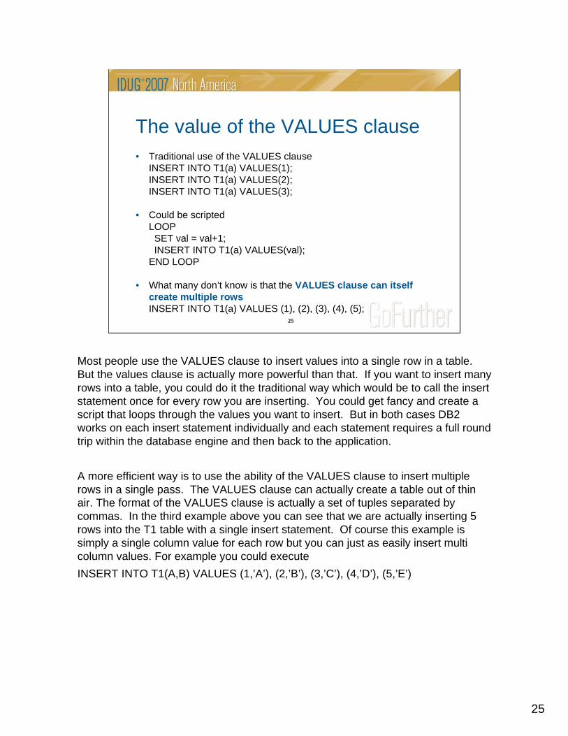
The value of the VALUES clause • Traditional use of the VALUES clause

INSERT INTO T1(a) VALUES(1);INSERT INTO T1(a) VALUES(2);INSERT INTO T1(a) VALUES(3);

• Could be scriptedLOOPSET val = val+1;INSERT INTO T1(a) VALUES(val);

END LOOP

• What many don’t know is that the VALUES clause can itself create multiple rowsINSERT INTO T1(a) VALUES (1), (2), (3), (4), (5);

Most people use the VALUES clause to insert values into a single row in a table. But the values clause is actually more powerful than that. If you want to insert many rows into a table, you could do it the traditional way which would be to call the insert statement once for every row you are inserting. You could get fancy and create a script that loops through the values you want to insert. But in both cases DB2 works on each insert statement individually and each statement requires a full round trip within the database engine and then back to the application.

A more efficient way is to use the ability of the VALUES clause to insert multiple rows in a single pass. The VALUES clause can actually create a table out of thin air. The format of the VALUES clause is actually a set of tuples separated by commas. In the third example above you can see that we are actually inserting 5 rows into the T1 table with a single insert statement. Of course this example is simply a single column value for each row but you can just as easily insert multi column values. For example you could executeINSERT INTO T1(A,B) VALUES (1,’A’), (2,’B’), (3,’C’), (4,’D’), (5,’E’)

26

26

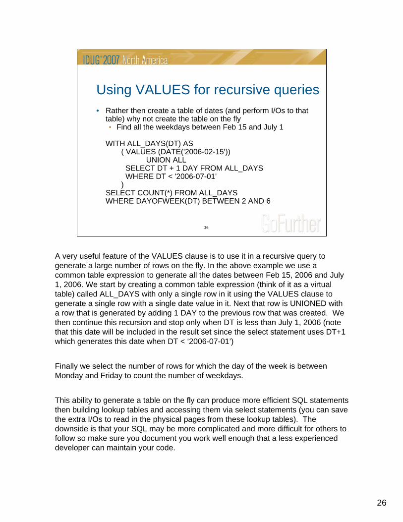
Using VALUES for recursive queries• Rather then create a table of dates (and perform I/Os to that

table) why not create the table on the fly• Find all the weekdays between Feb 15 and July 1

WITH ALL_DAYS(DT) AS( VALUES (DATE('2006-02-15'))

UNION ALLSELECT DT + 1 DAY FROM ALL_DAYSWHERE DT < '2006-07-01'

)SELECT COUNT(*) FROM ALL_DAYS WHERE DAYOFWEEK(DT) BETWEEN 2 AND 6

A very useful feature of the VALUES clause is to use it in a recursive query to generate a large number of rows on the fly. In the above example we use a common table expression to generate all the dates between Feb 15, 2006 and July 1, 2006. We start by creating a common table expression (think of it as a virtual table) called ALL_DAYS with only a single row in it using the VALUES clause to generate a single row with a single date value in it. Next that row is UNIONED with a row that is generated by adding 1 DAY to the previous row that was created. We then continue this recursion and stop only when DT is less than July 1, 2006 (note that this date will be included in the result set since the select statement uses DT+1 which generates this date when DT < ‘2006-07-01’)

Finally we select the number of rows for which the day of the week is between Monday and Friday to count the number of weekdays.

This ability to generate a table on the fly can produce more efficient SQL statements then building lookup tables and accessing them via select statements (you can save the extra I/Os to read in the physical pages from these lookup tables). The downside is that your SQL may be more complicated and more difficult for others to follow so make sure you document you work well enough that a less experienced developer can maintain your code.

27

27

INSERT, UPDATE, DELETE from SELECT

• Find the 50 oldest transactions from the ORDERS table and deletethem

DELETE FROM (SELECT ORDER_ID FROM ORDERS ORDER BY TRANSACTION_DATE FETCH FIRST 50 ROWS ONLY)

• Find any duplicates in a table and delete one of them

DELETE FROM ( SELECT ROWNUMBER() OVER

(PARTITION BY ADDRESS ORDER BYLAST_NAME,FIRST_NAME)

FROM CUSTOMER ) AS ADDR(ROWNUM) WHERE ROWNUM>1

How often does your application first SELECT data and then perform an INSERT/UPDATE/DELETE directly on that row. For example, SELECT the values out of a table, pass that information on to other parts of your application and then Delete that row that you selected. This requires two passes of the data and two round trips from the application to the database and back again. Now you can combine these two statements into a single statement. This not only performs just one trip inside the engine but it also can help avoid locking situations (like deadlocks with other applications).

In the first example above we fetch the 50 oldest orders by sorting the results by transaction_date and fetching the first 50 rows only and this is passed directly to the DELETE statement.

The second example is a very efficient deduplicator statement. We fetch the rows out of the address and assign a row number to each row. The partition by clause resets the row number back to 1 every time the address value changes. Now if there are any rows that have a rownum of 2 or higher then there must have been a duplicate address in the result set. The order by clause lets me decide which address I want to keep (i.e. which address will be assigned the rownum value of 1). In this case I simply decide the address that has the lowest value for last_name,first_name.

28

28

SELECT from INSERT, UPDATE, DELETE

• Insert new rows into a table and pass those rows back to the application • after triggers fire and generated columns are materialized

SELECT * FROM FINAL TABLE (INSERT INTO X VALUES …..)

• Instead of select next ordernum then insert in 2 stmts, do it in 1

SELECT ordernum INTO :ordernumFROM NEW TABLE(INSERT INTO orders(ordernum,…) VALUES(NEXT VALUE FOR orderseq, ...))

• Delete rows from a table and return their values to the application

SELECT * FROM OLD TABLE(DELETE FROM employee WHERE emp_id = 12345)

Similar to the previous slide, here we can now SELECT directly from an INSERT, UPDATE or DELETE statement. Often times we will have an application that inserts values into a table and then immediately selects that row back out to process further (for example to find the value of the generated columns and pass them back to the application. Rather then going back to the database twice, you can now SELECT directly from an INSERT.

The first example shows a simple select of the row(s) that are inserted into table X. The results of the select are the rows inserted after any triggers fire or columns are generated. Note that the SELECT * will return all the columns even if the insert statement is only inserting selected column values and letting other columns default.

The second example is a classic example in which you insert a row using a sequence number to generate the next order number. The select statement returns that order number back to the application (for further processing perhaps) without having to go back into the database engine to retrieve that row.

In the final example we see a SELECT from a DELETE statement. Using the OLD TABLE statement you see the value of the row before the action is taken. So in this case you see the value of the row before the DELETE takes place. This allows you to select a row, return it to the application and delete that row all in a single statement.

29

29

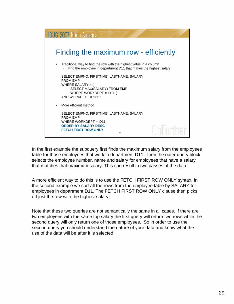
Finding the maximum row - efficiently• Traditional way to find the row with the highest value in a column

• Find the employee in department D11 that makes the highest salary

SELECT EMPNO, FIRSTNME, LASTNAME, SALARYFROM EMPWHERE SALARY = (

SELECT MAX(SALARY) FROM EMPWHERE WORKDEPT = 'D11' )

AND WORKDEPT = 'D11'

• More efficient method

SELECT EMPNO, FIRSTNME, LASTNAME, SALARYFROM EMPWHERE WORKDEPT = 'D11'ORDER BY SALARY DESCFETCH FIRST ROW ONLY

In the first example the subquery first finds the maximum salary from the employees table for those employees that work in department D11. Then the outer query block selects the employee number, name and salary for employees that have a salary that matches that maximum salary. This can result in two passes of the data.

A more efficient way to do this is to use the FETCH FIRST ROW ONLY syntax. In the second example we sort all the rows from the employee table by SALARY for employees in department D11. The FETCH FIRST ROW ONLY clause then picks off just the row with the highest salary.

Note that these two queries are not semantically the same in all cases. If there are two employees with the same top salary the first query will return two rows while the second query will only return one of those employees. So in order to use the second query you should understand the nature of your data and know what the use of the data will be after it is selected.

30

30


31

31

Check the validity of your backups• Utility to check the validity of your backup• Process reads the backup image to ensure it can be

restored

db2ckbkp SAMPLE.0.DB2.NODE0000.CATN0000.20060327164925.001

[1] Buffers processed: #######Image Verification Complete - successful.

If you have trouble sleeping at night because you are thinking about your database backups and if they are really good, here is a way to help you sleep.

The check backup utility db2ckbkp will scan a backup image you pass to it, check the integrity of the pages in the backup and ensure the image is valid to be used in a restore operation. You can also use this utility to dump the backup header information which includes the release of DB2 that was used during the backup, if the image is compressed, if logs are included in the backup and much more.

32

32

Recover Database from only tablespace backups • Rebuild a database from tablespace level backups

• Never take a full backup again

• Restore one tablespace using REBUILD option• Creates “structure” for entire database without the

containers for other tablespaces• Then restore other tablespaces as needed• Then roll forward to point in time

• Opens restored tablespaces for use• Puts other tablespaces not restored into restore

pending state

New to DB2 9 is the ability to completely restore a database with only tablespace level backup images. Prior to DB2 9 a full restore operation required a full database backup image to start with. Now you simply need to restore the tablespaces you want (and of course you must at least restore the catalog tables) and you can then open up the database for access. Tablespaces not restored can be restored later or simply dropped if they are no longer needed.

33

33

Restartable RECOVER command• RECOVER command does restore and rollforward

as one operation• If it fails, prior to DB2 9 it had to start at the restore

operation• As of DB2 9, it will pick up from where it left off

• Even if it was in the middle of roll forward

• When interrupted, you can even change the point in time you want to recover to.

The RECOVER command can now pick up from where it left off and continue processing in the event it is interrupted. If it is the rollforward phase you can interrupt it and change the time to recover to prior to or after the original recovery time. You can move the time back as long as the rollforward has not already passed that point in time. This ability can be very useful in cases where, for example, there is a missing log file which causes the recover command to fail. You can either stop recovery at that point or fix the missing log file problem, reissue the recover command and it will pick up from where it left off and continue the rollforward processing.

34

34

Redirected Restore Script Builder• SET TABLESPACE CONTAINERS command can

be complex to run at a time when you what to finish quickly

• New command

RESTORE DATABASE … REDIRECT GENERATE SCRIPT

• Builds script to run a full redirected restore• Simply edit the script to change the container

paths and run the script

If you have ever had to run a redirected restore, you know how cumbersome it can be. You must first start the redirected restore operation, then run a series of SET TABLESPACE CONTAINER commands to redirect the older tablespaces to new container paths and then finally resume the redirected restore operation. Now in DB2 9 there is an automatic script generator that you can use. It will create all of the commands required to run a redirected restore including all of the SET TABLESPACE CONTIANER commands for each of the tablespaces. All you have to do at this point is edit the script to redefine the container paths and then run the script.

35

35


36

36

Compression• Dictionary based - symbol table for compressing/decompressing data• Dictionary per table stored within the permanent table object (~74KB)• Data resides compressed on pages (both on-disk and in bufferpool)

• Significant I/O bandwidth savings• Significant memory savings• CPU costs: Rows must be decompressed before being processed

for evaluation• Log data from compressed records in compressed format

• Repeating patterns within the data is the key to good compression. Text data tends to compress well because of recurring strings as well as data with lots of repeating characters, leading or trailing blanks

One of my personal favorite new features in DB2 9 is compression. The compression feature looks for repeating patterns in a table (or a partition of a table) and replaces those repeating patterns with a 12bit symbol. The pattern is stored in a dictionary (which is stored within the table itself). The amount of storage savings that we are seeing with DB2 9 compression is in the range of 65% to 75%. That is, a table may be only ¼ of the size after compression.

This can result in significant I/O savings when performing table scans, performing backups/restores or other operations that need to scan large portions of the table.The CPU overhead is relatively low when you take into account the amount of I/O savings you can gain. Overall workloads that are I/O bound are seeing significant performance improvements at the cost of a few extra percentages in terms of CPU utilization.

37

37

CompressionDictionary contains repeated information from the rows in the table

Compression candidates can be across column boundaries or within columns

WhitbyONTL4N5R402

……

opoulos01Dictionary

KatsopoulosZikopoulos …L4N5R4ONTWhitby20000500L4N5R4ONTWhitby10000510

500 …(02)20000Kats(02)10000510Zik

L4N5R4ONTWhitby10000510ZikopoulosL4N5R4ONTWhitby20000500Katsopoulos

PostalCodeProvinceCitySalaryDeptName

The best part of compression is that it can find repeating column values as well as patterns that appear as substrings of column values and patterns that cross column boundaries.

In the example above we see that DB2 can compress the substring ‘opoulos’ from the Name column. It can also compress out the City, Province and PostalCode columns from the table down into one 12bit symbol for each occurrence. This is what results in the high disk savings.

38

38

Real World Example

81% Sm

aller

78% Sm

aller

SALES FactTable

PRODUCTDimension Table

As a real world customer example, Autozone ran through some tests of the compression capabilities of DB2 9 with several of their data warehouse tables. In their test the Sales table shrunk by 81% and their largest dimension table shrunk by 78%.

39

39

Real World Example

42% Faster

In the same tests, Autozone then ran a test workload against the non compressed and compressed data and found that the workload ran 42% faster on the compressed data.

More details on the Autozone tests and quotes from them are available herehttp://www-306.ibm.com/software/swnews/swnews.nsf/n/hhal6qkqt5?OpenDocument&Site=

40

40

New Table Partitioning in DB2 9• What is Table Partitioning ?

• Storing a table in more than one physical object, across one or more table spaces

• Each table space contains a range of the data that can be found very efficiently

• Why?• Increase large table manageability• Increase table capacity limit• Improve SQL performance

41

41

Table Partitioning

64G

Partitioned Table 32K Partitions

A-Z

64G

A-C

64G

D-M

64G

N-Q

64G

R-Z

BackupLoad

Recover

BackupLoad

Recover

BackupLoad

Recover

BackupLoad

Recover

BackupLoad

Recover

BackupLoad

Recover

Single table

In this example you see a single table made up of a single table partition on the left side of the screen. With a 4k Page size in DB2 v8 this table is limited to 64GB in size and contains all the data for that table.

With partitioning you can have up to 32,000 partitions and the data in the table can be broken down and stored in different tablespaces. Each partition can grow up to 64GB and with the new large rid support you can go even higher per partition. The primary benefit is for table maintenance like more granular backup, load, recovery and easy roll-in/roll-out.

42

42

64G

Jan

Table Partitioning

64G

Feb

64G

Mar

64G

Apr

64G

May

64G

Jan

64G

June

ALTER TABLE DETACH

PARTITIONJAN

ALTER TABLEATTACH

JUNE

LOAD

64G

June

Logical View of Fact TableCREATETABLEJUNE

Detaching a partition turns that partition into it’s own table. To attach a new partition you create a table with the same definition, load it with data and then ATTACH it to the partitioned table.

The detach and/or attach commands act virtually instantaneously. Index keys for the detach are physically removed asynchronously in the background but as soon as the detach completes these index keys are logically removed (that is, an index scan will not see these keys). Similarly an attach occurs almost immediately and then the index keys are added with the set integrity command. Both the attach and the set integrity command allow full read/write access to the table while they occur.

43

43

Self Tuning Memory Manager• DB2 9 introduces a revolutionary memory tuning system

called the Self Tuning Memory Manager (STMM)• Works on main database memory parameters

• Sort, locklist, package cache, buffer pools, and total database memory

• Hands-off online memory tuning• Requires no DBA intervention

• Senses the underlying workload and tunes the memory based on need

• Can adapt quickly to workload shifts that require memory redistribution

• Adapts tuning frequency based on workload

STMM in DB2 9 allows for the database to allocate memory to various consumers (bufferpool, sortheap, etc) automatically based on need. This takes the tuning of shared memory out of the hands of the DBA from a day to day basis and allows DB2 to manage the complex calculations of which heap should have which amount of memory assigned to it.

The biggest benefit is that it continuously monitors itself and constantly adjusts memory allocations to maximize the performance of the system over time.

44

44

STMM in action – 2 database on 1 box

0

1000000

2000000

3000000

4000000

5000000

6000000

7000000

0 10000 20000 30000 40000 50000 60000 70000

Time (in seconds)

Mem

ory

(in 4

K P

ages

)

Second databasestarted

Second database stopped

On AIX and Windows (the 2 platforms where this memory sharing is available from the operating system) DB2’s self tuning memory manager (STMM) can share memory resources between to databases or two instances on the same server. In the above graph you see the memory consumed by one database (the pink line). After a period of time a second database on that same server is started and begins to consume memory (the blue line). As shown, the first database will give up memory so that the operating system does not suffer when both databases are running at the same time. After the second database is stopped, the first database reallocates that memory to itself (to it’s benefit).

Without this type of self tuning memory allocations, a fixed allocation would require that the first database under configure itself such that the operating system does not get into trouble when both databases are running simultaneously.

45

45

Summary• If you want:

• snippets of information on using new features• sneak previews of upcoming releases• information on announcements I find interesting

• Then• Subscribe to my blog (you will get 2 or 3 emails

per week).

46

46

Chris EatonIBM

[email protected]

Session: D01Top Tips from the DB2 Experts Blog

Author of

blogs.ittoolbox.com/database/technology

Documents

Top Tips from the DB2 Experts Blog - idug.org