Top performing banks: the benefits to investors

Greg Filbeck & Dianna Preece & Xin Zhao

# Springer Science+Business Media, LLC 2011

Abstract In this study, we examine whether superior accounting performance asreported in the annual ABA Banking Journal Top Performing Banks survey translatesinto higher investor returns. We observe that the announcement effect is morepronounced during the early years of the survey. For the entire survey period and forlater sub-periods in which bank holding companies (BHCs) are ranked based onreturn on equity (ROE), we observe statistically-significant superior holding periodreturns against both the S&P 500 index and in some cases a matched sample. Theseresults include raw and risk-adjusted returns as well as buy and hold abnormalreturns (BHARs). We obtain similar results after controlling for the market return,size, book-to-market ratio, and momentum factors.

Keywords Banks . Bank Holding Companies . Shareholder Returns . AccountingReturnMeasures

JEL G11 . G21

1 Introduction

Over most of the last two decades, bank financial performance has been remarkablyrobust. However, in early 2007 the industry hit a stumbling block with the subprime

J Econ FinanDOI 10.1007/s12197-011-9197-4

G. Filbeck (*) :X. ZhaoBlack Family Professor of Insurance and Risk Management, Sam and Irene Black School of Business,Penn State Erie, 286 Burke, Erie, PA 16563, USAe-mail: mgf11@psu.edu

X. Zhaoe-mail: xuz12@psu.edu

D. PreeceCollege of Business, University of Louisville, Louisville, KY 40292, USAe-mail: dianna.preece@louisville.edu

mortgage crisis. As a result, the banking sector, while improving, continues to facesignificant challenges. Lax lending standards, primarily in the real estate sector, leadto lower returns for many banks. Evidence of industry struggles includes the failureof Washington Mutual Inc., in late September 2008. The bank was sold to J.P.Morgan Chase. Washington Mutual had $307 billion in assets, making it by far thelargest bank failure in U.S. history (Sidel, Enrich and Fitzpatrick, September 26,2008). Washington Mutual, like many other banks, had significant exposure to sub-prime mortgage loans. In addition, PNC received $7.7 billion in federal funds in late2008 and orders to use it to purchase struggling National City, which it did for $5.58billion, a mere $2.23 a share. Perhaps even more remarkable are the September 2008takeovers of mortgage giants Fannie Mae and Freddie Mac by the U.S. governmentand the failure of Lehman Brothers.

As a result of this extraordinary turn of events, the strength of the banking sectoris of even greater concern to those who study and/or invest in bank stocks. The BaselCommittee on Banking Supervision is in the process of implementing capital andliquidity reforms to improve the resiliency of banks. Investors targeting opportunitiesin the stocks of financial institutions must identify those banks and bank holdingcompanies (BHCs) that are likely to earn superior returns despite industrychallenges. Investors need a reliable source of information regarding the healthand performance of financial institutions. A possible source of this information is theABA Banking Journal’s “Top Performing Banks” survey.

The ABA Banking Journal is published by the American Bankers Association.Editors published the first of the annual rankings survey in 1993. The financial

information in the survey is based on FDIC call report data. The 1994 survey states:“Our original intent in ranking the most profitable banks was to develop a list ofbanks whose earnings indicated consistently superior performance in traditionalbanking activities” (p. 36). As such, early surveys did not include BHCs. Beginningin 1999, the ABA opened the survey to include both banks and BHCs. This survey isimportant to investors because it draws attention to banks and BHCs that exhibit thestrongest accounting performance in the industry.

In this study, we examine whether superior accounting performance as reported inthe ABA Banking Journal rankings translates into higher investor returns. Weinvestigate both announcement-related returns associated with the annual survey’srelease as well as survey-to-survey holding period returns, on a raw and risk-adjusted basis.

2 Literature review

In the banking literature, there has been little examination of the question ofwhether strong accounting measures of financial performance translate to highershareholder returns. However, there is much written on the subject regardingindustrial firms. For example, Bernstein (1956) was among the first to warninvestors not to confuse good companies with good stocks. He examines whetherfirms classified as “growth companies” are actually “growth stocks” and concludesthat superior financial results do not necessarily follow being classified as a growthcompany.

J Econ Finan

Peters and Waterman (1982) use growth, size, and innovation as criteria forexcellence in their book, In Search of Excellence: Lessons from America’s Best RunCorporations. Their sample consists of firms that are large, continuously innovative,and superior financial performers (in terms of growth). However, the firms did notdemonstrate “excellence” upon subsequent investigation of share price performance.For example, Clayman (1987) and Kolodny et al. (1989) investigate the stock marketperformance of firms considered excellent by Peters and Waterman. Clayman (1987)finds that a sample of firms that had the worst combination of financial ratios thatwere the criteria used in the Peters and Waterman study significantly outperform, ona risk-adjusted basis, the Peters and Waterman’s excellent firms. She cites theprinciple of mean reversion as a possible explanation for her findings. Kolodny et al.(1989) find no significant differences in the risk-adjusted returns of the “excellent”firms compared with either the market index or a matched sample of firms.

Surveys have focused on other types of financial ratios as criteria for rankings.For example, beginning in 1997, CFO Magazine began ranking firms across 35industries based on the efficiency of working capital management. The CFOMagazine survey focuses on two financial measures: cash conversion efficiencyand days of working capital. Filbeck et al. (2007) find little relationship betweenreturn and the key working capital variables of the firms listed in the CFOMagazine survey.

With respect to banks, Olson and Pagano (2005), in a study of bank mergersduring 1987–2000, find that the acquiring firm’s sustainable growth rate is animportant determinant of the cross-sectional variation in the merged entity’s long-term operating and stock performance.

In the early years of the survey, the ABA used return on assets (ROA) to measurebank performance. However, there has been debate as to whether ROA is anappropriate measure of performance. Cates (1996) argues that asset-based returnmeasures like ROAwere adopted by financial institutions to measure performance inthe 1960s. He contends that in the “Ice Age” (i.e., 1960s) ROAwas an appropriatemeasure because bank revenues and expenses originated on the balance sheet. Inother words, bank returns were derived from making loans and buying securitieswith funds supplied by depositors. However, much of a bank’s profitability, and riskfor that matter, is increasingly associated with off-balance activities. Cates assertsthat asset-based return measures such as ROA are no longer pertinent because “thedenominator is no longer relevant to the numerator.” He argues that return on equity(ROE) is a better measure because shareholders underwrite both the on and off-balance sheet risks of the bank. As such, we argue that ROE is more relevant thanROA as a measure of return, and that shareholder returns will be higher in the sub-periods where ROE is the primary rank order criteria used by the ABA.

It is reasonable to assume that market analysts would incorporate historicaccounting-based metrics as one method in which to evaluate the worthiness of abank or BHC stock in a security recommendation. In addition, investors consider avariety of metrics in their decision-making processes regarding portfolio selections.While analysts are a primary source of information for investors (see Han and Wild1991 and Pownall et al. 1993), investors may also respond to other sources of“news” based on behavioral or “noise” factors. Statman (1999) and other researchershave considered alternative frameworks by which investors approach investment

J Econ Finan

decision making. He points out that some investors are prone to representativeness,employing strategies that chase past winners or associate good or well-runcompanies with good investments. We investigate whether investors pay attentionto the ABA’s list of top performing banks, one method that investors might employto identify firms as “good, or well-run,” in order to make investment decisions.Thus, our paper falls within this vein of research.

Because accounting performance measures should be related to shareholderreturns, we expect long-term returns to be higher for the Top Performing Banks thanfor either the S&P 500 or a matched sample of financial institutions, both on a rawand risk-adjusted return basis. We compare the returns of sample banks on a raw andrisk-adjusted basis to those of a matched-sample of banks and BHCs and to the S&P500. We also calculate long-term buy-and-hold abnormal returns (BHARs). Byinvestigating longer-term performance, we are able to test an ex-ante investmentstrategy. We examine whether an investor, using the survey to establish a portfolioand then rebalancing year-to-year to reflect changes in the survey, can use the TopPerforming Banks list to enhance portfolio returns. In addition, we examine thesample in more detail, considering only new institutions to the survey, banks thatrepeat in the survey or return to the survey and banks that fall off the survey. Thispaper fills a gap in the literature in that it relates accounting measures of success toinvestor returns.

3 The ABA Banking Journal’s top performing banks survey

Our paper is the first to explore the value of the ABA Banking Journal publication tothe investing public. Our work in this area in not unlike other researchers whoinitiate studies that investigate whether a particular survey of admirable/wellmanaged/top performing firms are also investor-worthy. Starting with Clayman(1987)’s work regarding the book “In Search of Excellence,” researchers haveattempted to determine which surveys are worth noticing and which are not. Ourresearch adds to this stream of the literature as we investigate what investors may(or may not) garner from the ABA Top Performing Banks survey. According tothe ABA Banking Journal, their publication has an audited circulation of 34,584.This ranks first in circulation among bank and savings bank publications,representing circulation to 96% of all commercial bank and savings institutions(http://www.ababj.com/images/pdfs/ababjmediakit_11_09.pdf). Ex-ante, we expectinvestors to pay attention to this survey based on its reputation as the leadingpublication in banking.

The criteria for selection to the Top Performing Banks list have evolved over time.The initial ABA ranking was based on a five-year average ROA (net ofextraordinary gains or losses) for banks having no more than 15% core capital anda ratio of total loans to total deposits greater than 30%. Modifications for breakingties were made in 1995 using a five-year average ROE. In addition, a ceiling onloans to total deposits of 125% was established to be eligible for the survey. In the1997 survey, the ABA recognized that ROE was receiving increased attention butdefended its use of ROA, stating “our focus is on individual banks, not BHCs, andon ROA, not ROE, so the rankings do not necessarily pinpoint which institutions

J Econ Finan

provide the highest returns for their investors, nor which banking organizations on aconsolidated basis are most profitable” (p. 37). In 1998, the ABA states “critics ofROA point to the growing importance of off balance-sheet items and claim that sourcesof fee income such as asset management, transaction processing, and investmentproducts have very little relation to average assets” (p. 31).

Finally, in 1999 the ABA made a major change in the financial measure used forrankings: they began using return on average equity (ROAE) for the larger categoryof banks, although ROA remained the benchmark used for smaller institutions(community banks). The ABA also began dividing banks into categories: those over$1B in total assets and those under $1B in total assets.

The categories of financial institutions expanded to three in 2000: banks andBHCs, thrifts, and specialty leaders. The ABA changed the criteria to include onlyinstitutions with assets greater than $1B, thereby excluding community banks fromthe survey. This is interesting in that it was these smaller, traditional bankinginstitutions that were the focus of the early surveys. This shift reflects a 180°turnaround from the ABA in less than 10 years and is indicative of the significantchanges in the banking industry as a whole during that period.

In 2002 banks and thrifts were combined due to the increasing overlap betweenthem. Most recently, in 2005, recognizing the increasing size of financial institutionsthrough growth and consolidation, the minimum floor for inclusion in the surveywas raised to $3B in assets.

The data reported in the ABA surveys are available to the public dating back to2001. However, it is available in a relatively inaccessible form—FDIC call reports.According to the FDIC website, the FDIC collects and stores Reports of Conditionand Income data submitted by all insured national and state nonmember commercialbanks and state-chartered savings banks on a quarterly basis. One of the effects ofthe ABA Banking Journal best performing banks survey is to make call report returndata more accessible to investors, at least for the subset of Top Performing Banks.Call report data are available but traditionally unwieldy to access and navigate.However, accessibility has improved in recent years.1 Given that the financialinformation contained in call reports is public, we examine whether the marketresponds to the more conveniently-packaged “news” in the ABA surveys.

In addition, we investigate whether strong profitability translates into highershareholder returns. We consider whether the market perceives the inclusion ofpreviously unlisted banks or BHCs to the survey as newsworthy. We also considerwhether the market response is greater for banks that repeat in the survey. In thisstudy we link the book value return measures extolled in the ABA’s surveys to actualshareholder returns. We investigate whether the market “notices” industry-specificrankings like those published by the ABA by measuring abnormal returns toincluded firms around the announcement of the Top Performing Banks via the

1 An interagency Call Modernization project was launched in 2001. It was a collaborative effort of theFDIC, the Federal Reserve Board and the Office of the Comptroller of the Currency to improve theprocesses and systems used to collect, validate, store and distribute call report data. Prior to themodernization, call report information was available via magnetic tape. This is relevant to our study in thatthe ABA survey first appears in 1993. The changes to the way the data is distributed occurred sometime in2003. This means that for the bulk of this study period, the data was relatively inaccessible (i.e. tape versusthe internet).

J Econ Finan

survey. We also explore the longer-term holding periods on a raw and risk-adjustedbasis associated with the banks named in the ABA survey.

4 Sample

The Top Performing Banks sample in this study is based on the ABA’s annual survey,the first of which was released to the press July 1, 1993.2 To be included in thesample, the firm must meet the following criteria:

1. The sample firms must have return records on the Center for Research on StockPrices (CRSP) Daily Combined Return File, 301 trading days (i.e., one tradingyear) immediately prior to the announcement date.

2. The sample firms must have return records on the CRSP Daily CombinedReturn File after the announcement date until the press release date of the nextsurvey.

3. The firm must have complete data on S&P’s Research Insight® (CompustatBank Annual file3).

The total number of observations related to banks, thrifts and BHCs named in theABA survey between 1993 and 2009 is 900.4 This sample represents 188 distinctbanks that appear on the ABA list from 1993 to 2009. Of these 188 banks, 60 banksappeared on the ABA list only once, 38 banks appeared only twice, and 90 banksappeared more than twice. Also, in the early years of the survey, many banks did nothave available data on CRSP and Compustat because they were privately held. Infact, because so many banks were privately held, only 75 banks of the 275 listed inthe first subperiod (1993–1998) met the selection criteria for the purpose of thisstudy. Across the 17 years of the survey, there are 597 listings that meet the selectioncriteria. These 597 banks and BHCs, some of which repeat in two or more surveys,constitute the overall sample. Table 1 reports the summary statistics of the TopPerforming Banks sample.

Because the selection criteria underwent significant changes in 1999 and 2001,we divide the sample into three sub-periods: 1993–1998, 1999–2000 and 2001–2009. This sub-period division method (especially for the first sub-period) is alsobased on the fact that prior to 1999, the ABA focused on individual banks, notBHCs. This accounts for the disproportionate increase in the size of total assets after1999. In addition, the mean size of BHCs in the 2001–2009 sub-sample is influencedby the increase in the minimum floor value to $3 billion in 2005. Within the 2001–2009 sub-sample, we also break out results for the period, 2007–2009, This timeperiod is singled out due to the fact that the banking sector was undergoing a periodof extreme turmoil, affecting returns across the industry.

2 The ABA continues to publish the survey each year.3 The Compustat Bank Annual file contains annual accounting data on approximately 638 of the leadingUnited States banking institutions.4 There are a total of 900 announcements during the sample period: 25 announcements for 1993, 50annual announcements during the time period of 1994–1998, 100 annual announcements for the timeperiod 1999–2002, 50 annual announcements in 2003 and 2004, and 25 annual announcements for thetime period 2005–2009.

J Econ Finan

Table

1Descriptiv

eStatistics

Variable

Sam

plesize

Mean

Standarddeviation

Percentile

Min

2550

75Max

a.Descriptiv

estatisticson

whole

sampleandsub-samples

Whole

sample

597

Totalasset(m

illions

$s)

39,673

.49

140,13

5.25

278.12

2,198.95

5,726.96

18,120

.19

1,884,318.00

Year

1993–199

875

TotalAsset

(millions

$s)

5,153.93

10,085

.07

1,008.34

1,919.39

2,717.36

5,057.71

89,155

.93

Previous5-yr

ROA

1.60

0.20

0.62

1.46

1.60

1.75

2.06

Previous5-yr

ROE

19.93

5.43

0.15

17.94

21.42

23.42

32.60

Year

1999–200

018

2

TotalAsset

(millions

$s)

34,242

.41

89,507

.99

1,001.00

1,859.00

5,825.00

27,870

.00

716,93

7.00

Previousyear

ROA

1.46

0.39

0.01

1.22

1.43

1.65

3.62

Previousyear

ROE

18.26

3.80

0.17

16.12

17.67

20.06

36.91

Year

2001–200

934

0

TotalAsset

(millions

$s)

49,295

.78

169,66

9.87

278.12

2,542.87

6,999.54

21,078

.76

1,884,318.00

Previousyear

ROAA

1.55

0.51

0.01

1.25

1.47

1.76

5.42

Previousyear

ROAE

19.51

5.90

0.14

16.77

19.09

21.21

81.23

Year

2007–200

963

TotalAsset

(millions

$s)

85,459

.93

269,66

1.89

3,161.19

5,467.45

12,088

.69

36,059

.01

1,884,318.00

Previousyear

ROAA

1.47

0.48

0.01

1.17

1.40

1.75

2.82

Previousyear

ROAE

16.52

5.50

0.14

13.92

16.68

19.55

29.14

New

Listin

gSam

ple

188

TotalAsset

(millions

$s)

21,090

.45

68,588

.72

1,000.61

1,482.87

2,875.00

9,766.19

716,93

7.00

J Econ Finan

Table

1(con

tinued)

Variable

Sam

plesize

Mean

Standarddeviation

Percentile

Min

2550

75Max

New

Listin

gROESam

ple

165

TotalAsset

(millions

$s)

23,233

.69

72,698

.08

1,000.61

1,482.87

2,875.00

10,539

.90

716,93

7.00

RepeatWinnerSam

ple

318

TotalAsset

(millions

$s)

43,461

.55

151,69

3.36

278.12

2,502.12

6,687.38

19,992

.24

1,884,318.00

ReturnedWinnerSam

ple

87

TotalAsset

(millions

$s)

61,783

.17

181,97

9.87

1,028.53

3,279.46

8,198.88

38,600

.41

1,494,037.00

Loser

Sam

ple

212

TotalAsset

(millions

$s)

42,938

.83

170,03

2.42

1,000.61

1,906.00

4,733.45

19,036

.25

1,884,318.00

b.Descriptiv

estatisticson

topperformingbanksandits

matched

sample

TopPerform

ingBanks

597

MarketCapitalization(m

illions

$s)

5,428.07

14,803.51

19.53

438.39

1,178.78

3,224.81

120,091.45

Loanto

DepositRatio

0.75

0.37

0.00

0.64

0.83

0.97

1.96

Previousyear

ROA

(%)

2.11

0.62

0.56

1.73

2.05

2.45

7.71

Previousyear

ROE(%

)17

.56

4.21

5.03

15.08

17.24

19.16

55.37

Matched

Sam

ple

597

MarketCapitalization(m

illions

$s)

3,750.93

8,452.57

19.70

389.15

1,014.69

2,753.76

73,703.17

Loanto

DepositRatio

0.79

0.36

0.00

0.73

0.87

0.99

1.84

Previousyear

ROA

(%)

1.61

0.80

−4.02

1.25

1.65

1.98

5.97

Previousyear

ROE(%

)11.37

5.96

−38.06

9.42

12.31

14.71

27.84

J Econ Finan

To test how inclusion in (or removal from) the list of Top Performing Banks hasan effect on stock returns, we further divide the sample into five sub-samples: “newlisting,” “new listing ROE,” “repeat winners,” “returned winners,” and “loser” banksamples. The “loser” sample includes those financial institutions that have beendropped from the Top Performing Banks list. We consider these sub-samples in orderto determine if there is one or more groups driving the results. More specifically,investigating these sub-samples allows us to examine whether there are aspects ofthe survey itself that convey more information than the release of the overall survey.One might expect that the true information hits the market the first time a bankappears on the survey (i.e. a new listing). Alternatively, one could argue that it isonly after repeat appearances on the list that an institution is recognized by themarket as superior. These banks have a track record of superior performance.Investors are more assured that the bank’s appearance on the list is not a function ofextraordinary, one-time factors. Also, since we argue that ROE is the more relevantreturn measure, we also consider the sub-sample of newly listed financial institutionsafter 1999 when ROE became the ABA’s performance measure of choice. As such,we look separately at this repeat winner sub-sample. Finally, the loser samplecontains banks that fail to appear in a survey after being listed the previous year. Weexpect that market participants will sell these stocks upon release of the survey andthat the announcement effect will be negative.

The five sub-samples are described as follows:

& New listing sample. The new listing sub-sample contains only firms that are notpreviously listed in the survey. We include all stocks listed in 1993 since it is thefirst year of the survey. For subsequent years, we include only firms that appearon the list for the first time.

& New listing ROE. The new listing ROE sub-sample is based on ROEs of thebanks included in the survey following the 1999 change of the ABA criterion.

& Repeat winners. The repeat winner sub-sample contains only firms that alsoappear in the previous year’s survey.

& Returned winners. The returned winner sub-sample contains firms that hadappeared in a previous year’s survey, dropped off the list and then re-appeared inthe survey.

& Loser sample. The loser sub-sample contains the financial institutions that havebeen deleted from the previous year’s list.

Table 1a reports the average total assets for these sub-samples. As expected, giventhe size criterion changes of the ABA, in general repeat winners and returnedwinners have higher total assets than the new listing banks and loser bank samples.Notice that ROA is approximately 1.5%, and that ROE is slightly less than 20% foreach sub-sample. Assets range from a minimum of $278 million to approximately$1.9 trillion.

Next, we construct a matched sample on the basis of the institutional size, regionand loan-to-deposit ratio. Banks are heavily regulated as well as heavily leveraged.They have federally insured debt (i.e., deposits) and many are perceived as too-big-to-fail. Matching banks and BHCs against traditional industrial firms is thereforeinappropriate. As such, we match the bank stocks of the ranked firms with financialinstitutions in the same region. We retrieve all the bank financial information from

J Econ Finan

the Compustat Bank Annual file each year and divide them into four regions5

(Northeast, South, Pacific and Midwest) according to the headquarter location.For each year, we gather year-end t (year t is the event year when the survey is

released) market capitalization, total loan and total deposit data for all availablebanks and BHCs. We calculate the loan-to-deposit ratio for all available banks eachyear. The potential universe of matching firms consists of all remaining banks andBHCs (i.e. not on the Top Performing Banks list) that are in the same region and alsohave available data from CRSP and the Research Insight® Annual Bank file. If abank or BHC in the sample previously appeared on the ABA list, it is excluded fromthe potential set of matching firms. Finally, for each bank or BHC in the sample, weselect the bank or BHC from the remaining financial institutions with the closestmarket capitalization and loan-to-deposit ratio located in the same region.6 We repeatthe procedure for each study year. Table 1b reports descriptive statistics for the TopPerforming Banks sample and the matched sample. The Top Performing Banks havea slightly larger market capitalization, but a similar average loan-to-deposit ratiocompared to the matched institutions. The larger size of the Top Performing Banks isprimarily driven by the much higher market capitalization in the top quartile of thesample. As expected, the Top Performing Banks have higher previous year ROA andROE, on average, than the matched sample counterparts.

5 Methodology

5.1 Short-run market impacts

We hypothesize that there will be a positive market reaction to the release of theABA best performing banks list. Alternatively, the market may not respond at all tothe announcement, which would indicate that either the market does notincrementally value the information contained in the survey or that the “news”contained in the survey is already fully valued.

The ABA Banking Journal chief editor indicated in a phone conservation that thepublication is typically mailed out around the first of the month in which it is dated(e.g., July 1 for July publication). Typically, recipients get the publication within3 days, but occasionally delays could push delivery out one or more days. The ABAalso posts a digital image of the publication on the ABA website approximately1 week after the publication is mailed. While we identify July 1, 19937 as t=0 for thefirst year of publication, there is some likelihood that a few financial institutions maybe notified in advance of their inclusion in the list. It is possible that bankmanagement might leak the information to the press or to the bank’s shareholders afew days prior to the event date. This would argue for a price run-up leading up to

5 We combine the “Mountain” region and “Territories” into the “Pacific” region due to small sample sizes.6 The ABA uses the loan-to-deposit ratio as a screening criterion for the survey because generallyspeaking, the higher the loan to deposit ratio, the higher the risk of the institution. Banks of similar size,from the same region and with similar loan-to-deposit ratios are likely to be similar with respect to risk. Ifa top performing bank has missing information needed to calculate the loan to deposit ratio, we matchonly on the basis of market capitalization and geographic region.7 The event dates are July 1 from 1993 to 1998, June 1 from 1999 to 2006 and May 1 from 2007 to 2009.

J Econ Finan

the announcement date. The publication may also take a few days to reachrecipients and investors are likely to receive the publication on different days.Therefore, identifying a specific event date is somewhat problematic. Our studyis not unique in this regard. In the extreme, Huberman and Regev (2001) trackedthe stock market reaction over a 15-month “event window” while studying theresponse to EntreMed’s potential development of cancer-curing drugs. Similarly,events such as changes in bond ratings are typically studied over severalannouncement windows leading up to the actual event (e.g., Goh and Ederington1993). We also look at longer event windows based on potential differences in thereceipt of the publication and thus follow the Goh and Ederington methodology foridentifying event windows.

We test the share price response to the release of the survey beginning 15trading days prior to the date of the publication by cumulative abnormal returns(CARs). Expected returns are estimated using the market model during theinterval (−15, +15). Estimates of the parameters are calculated for the period(−326, –71). We follow Dodd and Warner (1983) and employ standard event-study methodology.

5.2 Long-term stock return performance

We also examine the long-term return performance of the Top Performing Bankssample after each publication date. Numerous researchers including Barber and Lyon(1997), Fama (1998), and Loughran and Ritter (1995) have shown that themagnitude, and sometimes even the sign, of the long-run abnormal returns aresensitive to alternative measurement methodologies. To address this issue, weexamine long-run performance using a variety of methodologies.

Initially we test the long-run stock performance of the sample by forming aportfolio consisting of the Top Performing Banks on July 1, 1993. This portfolio is“held” until the release of the next publication, in this case on July 1, 1994, at whichpoint the portfolio is rebalanced to reflect the inclusion of newly listed financialinstitutions and the elimination of banks and BHCs not appearing on the subsequentlist. The sample process is used for subsequent holding periods.

Three types of benchmark portfolios are used to test the abnormal returns of theTop Performing Banks sample: the S&P 500 index and a matched sample. Todetermine abnormal returns, we calculate both the traditional CARs and buy-and-hold abnormal returns (BHARs) over the holding period until the next publicationrelease date. In addition, we calculate a variety of risk-adjusted performancemeasures. Last, we employ the Fama-French 3-factor and 4-factor models to testthe abnormal returns. The methodologies and test results are discussed in thefollowing sections.

5.2.1 Long-term CARs: annualized raw returns

We define Rit as the date t simple return on the Top Performing bank i, E(Rit) as thedate t expected return for the matched bank or BHC and ARit=Rit–E(Rit) as the day tabnormal return. In this case, we use the S&P 500 daily returns, bank portfoliovalue-weighted portfolio returns and stock i’s matched return as E(Rit). Cumulating

J Econ Finan

across T trading days (i.e., T is the number of trading days until the next press releasedate) yields the CAR:

CARiT ¼XT

t¼1

ARit ð1Þ

For each stock in the Top Performing Banks sample, we calculate its CARcompared to the benchmark portfolio over the holding period and use the pairedt-test to determine whether the CAR is significantly different from zero. We reportthe raw returns for the entire time period (the release date of the 1993 publicationto December 31, 2009), for the four sub-periods (1993–1998, 1999–2000, 2001–2009and 2007–2009) and for the five sub-samples (new listing, new listing ROE, repeatwinners, returned winners and “loser” banks).

5.2.2 Risk-adjusted performance measures

We also calculate three risk-adjusted performance measures. The Sharpe reward-to-variability ratio (Sharpe 1966, 1994) is a measure of return per unit of total risk. It isthe appropriate risk-adjusted return measure when the portfolio being analyzed isbeing held by a less diversified investor. Sharpe (1994) argues that for ex-postevaluation of performance, the differential form of the ratio should be used, whichappears below:

Sharpe Index¼ d1sd1

; ð2Þ

where:

d1 mean holding period difference between the Top Performing Banks sample (orS&P 500 or matched sample) and the T-bill return, calculated over each day

sd1 the sample standard deviation of the daily return differences

We also calculate the Treynor reward-to-volatility ratio (Treynor 1965), whichmeasures return per unit of systematic risk. It is the more appropriate measure ofrisk-adjusted return for a diversified investor less exposed to company-specific risk.It is calculated:

Treynor Index ¼ d1b; ð3Þ

where:

d1 the mean holding period difference between the portfolio (or the matchedsample) and the T-bill return, calculated over each day

β portfolio beta, or market beta (βm=1)

Betas are calculated by regressing daily excess returns for both the TopPerforming Banks sample and the matched sample portfolios against market excessreturns. The regressions to calculate the betas match with the holding periods underinvestigation (e.g., the beta calculated for the analysis of the 2005 holding periodwas based on daily return data for the 2005 period).

J Econ Finan

Jensen’s (1968) alpha, indicates whether a portfolio exhibits above or belowaverage risk-adjusted returns on an absolute basis. Jensen’s alpha, α, is the interceptterm of the regression of the excess returns on a portfolio of the Top PerformingBanks against the excess returns of the market:

Rit � Rft ¼ a þ b Rmt � Rft

� �þ eit; ð4ÞA positive (negative) alpha is consistent with a portfolio of undervalued

(overvalued) securities.The information ratio (IR) is defined as the active return divided by tracking error,

where active return is the difference between the return of the portfolio and thereturn of a selected benchmark (i.e., matched firms or S&P 500 Index in this study),and tracking error is the standard deviation of the active return. The IR is:

IR ¼ RP � RB

SD RP � RBð Þ ð5Þ

The information ratio is often used to gauge the active management skill ofmutual fund and hedge fund managers by measuring the expected active return ofthe manager’s portfolio divided by the amount of active risk that the manager takesrelative to the benchmark.

5.2.3 Buy-and-hold Abnormal Returns (BHARs)

Long-term performance is also assessed using BHARs. Building on the work ofRitter (1991) and Barber and Lyon (1997), we argue that BHARs may be used toaddress different issues regarding portfolio performance. A BHAR is the differencebetween the return on a buy-and-hold investment in a bank or BHC of interest lessthe return on a buy-and-hold investment in a similar asset/portfolio. Specifically,BHARiT is calculated as:

BHARiT ¼YT

t¼1

1þ Rit½ ��YT

t¼1

1þ E Ritð Þ½ � ð6Þ

Where:

Rit the daily returns of stock i from Top Performing BanksE(Rit) the expected return of bank i (i.e., the daily returns of a matched bank

from the matched sample)T the number of days in the holding period.

BHARs can overcome several biases inherent in estimating long-term CARs.Barber and Lyon argue that matching sample firms to control for size and book valueof equity to market value of equity (BE/ME) ratios will correct for possible sourcesof misspecification. Because of the special characteristics of banks, we use thematched sample (matched based on the institutional size, region and loan-to-depositratio) as our benchmark portfolio.

For both the Top Performing Banks and their matched sample, daily returns arecalculated and cumulated between survey releases and over all survey periods usingthe geometric mean of the equally-weighted daily returns.

J Econ Finan

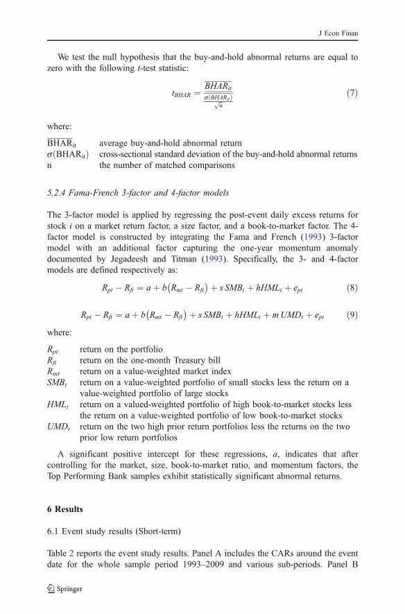
We test the null hypothesis that the buy-and-hold abnormal returns are equal tozero with the following t-test statistic:

tBHAR ¼ BHARit

s BHARitð Þffiffin

pð7Þ

where:

BHARit average buy-and-hold abnormal returns BHARitð Þ cross-sectional standard deviation of the buy-and-hold abnormal returnsn the number of matched comparisons

5.2.4 Fama-French 3-factor and 4-factor models

The 3-factor model is applied by regressing the post-event daily excess returns forstock i on a market return factor, a size factor, and a book-to-market factor. The 4-factor model is constructed by integrating the Fama and French (1993) 3-factormodel with an additional factor capturing the one-year momentum anomalydocumented by Jegadeesh and Titman (1993). Specifically, the 3- and 4-factormodels are defined respectively as:

Rpt � Rft ¼ aþ b Rmt � Rft

� �þ s SMBt þ hHMLt þ ept ð8Þ

Rpt � Rft ¼ aþ b Rmt � Rft

� �þ s SMBt þ hHMLt þ mUMDt þ ept ð9Þwhere:

Rpt return on the portfolioRft return on the one-month Treasury billRmt return on a value-weighted market indexSMBt return on a value-weighted portfolio of small stocks less the return on a

value-weighted portfolio of large stocksHMLt return on a valued-weighted portfolio of high book-to-market stocks less

the return on a value-weighted portfolio of low book-to-market stocksUMDt return on the two high prior return portfolios less the returns on the two

prior low return portfolios

A significant positive intercept for these regressions, a, indicates that aftercontrolling for the market, size, book-to-market ratio, and momentum factors, theTop Performing Bank samples exhibit statistically significant abnormal returns.

6 Results

6.1 Event study results (Short-term)

Table 2 reports the event study results. Panel A includes the CARs around the eventdate for the whole sample period 1993–2009 and various sub-periods. Panel B

J Econ Finan

includes the sub-sample CARs. The results are mixed. The entire survey period (0,1) CAR (i.e. 1993–2009) is 0.23% and is significant at the 5% level. The 1993–1998subperiod event window CAR is 0.84% and is significant at the 1% level. Inaddition, the CAR for the 1993–1998 period overall event window (−15, 15) is2.23% and is also significant at the 1% level. However, for the entire 1993–2009period and the 1999–2000 subperiod, the results are insignificant over the (15, 15)window. In addition, for the subperiod 2001–2009, there is no reaction to the releaseof the survey, although for the entire event window (−15, 15), the reaction isnegative and statistically significant at the 1% level.8 However, upon furtherinvestigation, the result for this sub-period appears to be driven by the 2007–2009period, associated with the recent global financial crisis. It is not surprising that thebanking industry suffered more than the overall market due to the nature of thecrisis. In fact, in the 2007–2009 period the magnitude of the CARs over the entire

8 The run-up (−15, −1) window for the 2001–2009 sub-period is also negative and significant. This resultis largely due to the 2007–2009 period, which also has a significant negative run-up.

Table 2 Cumulative abnormal returns (CARs) around the event date for top performing banks

Whole Sample Year 1993–1998 Year 1999–2000 Year 2001–2009 Year 2007–2009

New Listing New Listing ROE Repeat Winner Returned Winner Loser

Interval CAR t-stat CAR t-stat CAR t-stat CAR t-stat CAR t-stat

Panel A. Cumulative abnormal returns (in percentage) for different sub-periods

(−15, −1) 0.75 2.20b 1.50 1.91 3.88 5.09a −1.48 −3.57a −3.32 −2.35b

(0, 1) 0.23 2.16b 0.84 2.96a 0.42 1.65c 0.02 0.13 0.11 0.33

(2, 15) −0.86 −2.95a −0.10 −0.24 −4.42 −7.14a −0.38 −1.01 −5.73 −5.05a

(−15, 15) 0.12 0.30 2.23 2.90a −0.12 −0.16 −1.84 −2.94a −8.94 −4.26a

Panel B. Cumulative abnormal returns (in percentage) for different sub-samples

(−15, −1) −0.19 −0.33 −0.39 −0.60 1.00 2.10b 0.13 0.14 −0.86 −1.27(0, 1) 0.04 0.22 −0.02 −0.11 0.29 2.09b 0.24 1.07 0.55 2.56b

(2, 15) −1.00 −1.98b −0.86 −1.53 −1.65 −4.15a −1.79 −2.10b −2.37 −3.85a

(−15, 15) −1.15 −1.48 −1.28 −1.45 −0.36 −0.60 −1.41 −1.24 −2.69 −2.64b

Table 2 reports the results of the event study for the Top Performing Banks. Panel A shows the cumulativeabnormal returns (in percent) around the event date for different sub-periods, and Panel B shows thecumulative abnormal returns (in percentage) around the event date for the different sub-samples. We testthe share price response to the release of this survey beginning 15 days prior to the event date bycalculating abnormal returns (ARs) and cumulative abnormal returns (CARs). Expected returns areestimated from the market model. Expected returns are estimated from the market model. Expected returnsare estimated during the interval (−15, 15) and estimates of the parameters are calculated for the tradingday period (−301, –46) using 255 trading day year. We follow Dodd and Warner (1983) and employ event-study methodologya Statistically significant at 1% levelb Statistically significant at 5% levelc Statistically significant at 10% level

J Econ Finan

event window is five times greater than the rest of the sub-period (2001–2006).This implies, not surprisingly, that the financial crisis had a significant impact onbank returns.9

In general, over the entire event window, the Table 2, the results in Panel Aindicate that the survey had the largest share price impact in the period between 1993and 1998. There are at least two possible explanations for the significant results inthe earliest sub-period. First, the survey was new. The early focus was on individualbanks, many of which may have “flown under the radar” of investors and analystsprior to the survey’s initiation. Remember the initial surveys include banks, notBHCs. The institutions included in the early years of the survey are substantiallysmaller than in subsequent years. Also, any survey, including this one, may have agreater impact in the early years (and especially the first year) since the informationis new. Second, smaller banks are less likely to be covered by analysts; so again, thenews may have more impact than if the focus had been on large, money-centerBHCs. In addition, information is more readily available to investors regarding allfirms, including banks, than it was 15 years ago. Investors may rely less on newinformation garnered from industry publications such as the ABA Banking Journalthan in the past.

As indicated in Panel B, over the same interval (−15, 15), the “loser” subsampleexhibits a CAR of −2.69%, which represents a statistically significant loss at the 1%level. Oddly however, the loser sample CAR in the (−1, 0) window is a positive0.55% and is significant at the 5% level. A possible explanation is that investors’reactions are delayed as they process “what’s missing” from one survey to the next.This interpretation is supported by the (2, 15) event window results. The (2, 15)CAR is −2.57%, significant at the 1% level. This implies investors may haveevaluated the firms after the survey release and sold the banks and BHCs in theirportfolios that had fallen off the ABA list.

The lack of statistically-significant abnormal returns of the new listing bankssample seems surprising, but might be explained by the fact that about 44% of ournew listing sub-sample (82 out of 188) is added in 1999 (with the inclusion ofBHCs). On closer inspection we find that over the 1999 (−15, 15) event window, thebanking industry exhibits a −1.8% CAR while the CRSP equally-weighted marketindex exhibits a 3.29% CAR. Thus, the event study results of new listing banks maybe driven by the industry underperformance compared with the market index. Also,the repeat winner sample does exhibit a statistically significant positive CAR of0.29% (significant at the 5% level).

In sum, we find that for the “loser” sub-sample, the event study results indicate aconsistent negative share price response over the entire event window (−15, 15).Based on these findings we conclude that tactical, short-term traders are rewardedshort-selling or by removing any bank or BHC that does not appear in the rankingsafter being a part of the Top Performing Banks survey the previous year (i.e. the“loser” sample). Also, the 2007–2009 period magnifies these findings relative to therest of the subperiod (2001–2006).

9 We have separately examined the period 2001–2006 and the results do not change our overallconclusions. These results are available upon request.

J Econ Finan

In sum, use of the survey itself as a basis for constructing a short-term portfoliodoes produce ambiguous results, but is useful and consistent with respect totwofindings (1) during the early years of the survey, (2) for short-sellers who gain asthe market reacts negatively to those banks that are dropped from the survey.

6.2 Raw and risk-adjusted holding period returns (Long-term)

Tables 3 and 4 report the raw holding-period returns and risk-adjusted returns for theTop Performing Banks sample for different sub-periods and sub-samples, respec-tively. Table 3, Panel A reports the raw holding-period returns for the TopPerforming Banks sample and the benchmark portfolios (i.e. the S&P 500 returns

Table 3 Raw and risk-adjusted returns of the top performing banks sample for the sub-periods

Whole Sample Year1993–1998

Year1999–2000

Year2001–2009

Year2007–2009

Panel A. Cumulative raw returns (%) and CARs (%)

Cumulative raw returns (%)

Top Performing Banks (1) 12.816 18.807 13.159 11.605 −0.263Matched (2) 12.597 24.046 11.259 11.154 −7.550CAR: (1)–(2) 0.220 −5.239b 1.900 −1.205 7.287

S&P 500 Index (3) 1.078 16.745 0.055 −0.012 −5.025CAR: (1)–(3) 11.738a 2.062 13.104a 12.810a 4.762

Panel B. Risk-adjusted performance measures

Sharpe measure

Top Performing Banks (1) 0.017 0.035 0.013 0.017 −0.002Matched (2) 0.015 0.042 0.010 0.014 −0.008S&P 500 Index (3) −0.006 0.055 −0.016 −0.010 −0.015Treynor measure

Top Performing Banks (1) 0.049 0.100 0.055 0.044 −0.006Matched (2) 0.047 0.124 0.050 0.039 −0.026S&P 500 Index (3) −0.008 0.049 −0.021 −0.013 −0.030Jensen’s alpha

Matched as Benchmark 0.027a 0.045 0.010 0.031b 0.021

S&P 500 Index as Benchmark 0.048a 0.029 0.046a 0.054a 0.033

Information ratio

Matched as Benchmark 0.000 −0.009 0.002 0.001 0.008

S&P 500 Index as Benchmark 0.023 0.005 0.022 0.027 0.007

Table 3 reports the raw and risk-adjusted returns of the Top Performing Banks sample compared to S&P500, bank industry and matched sample for different sub-periods. Panel A reports the annualized rawreturns for the Top Performing Banks sample and benchmark portfolios (i.e., S&P 500 returns, bankindustry portfolio returns and matched sample returns). For each stock in the Top Performing Bankssample, we calculate its CAR compared to benchmark portfolio over the holding period and use the pairedt-test to determine whether its CAR is significantly different from zero. Panel B shows calculations for thefour risk-adjusted performance measures: Sharpe measure, Treynor measure, Jensen’s alpha andinformation ratio. (a Statistically significant at 1% level; b Statistically significant at 5% level)

J Econ Finan

and the matched sample returns) over longer holding periods. When cumulative rawreturns for the Top Performing Banks sample are compared to those of the S&P 500, thecumulative raw returns of the former exceed their respective counterpart measures inevery holding period. In addition, in the first sub-period, the Top Performing Bankssample has significantly lower cumulative raw returns (at the 5% level) compared to thematched sample counterparts.

Table 4, Panel A shows that the returns exceed the S&P benchmark returns in allsub-samples as well (significant at the 1% level for each sub-period). Table 4indicates that when the Top Performing Banks sample returns are compared to thoseof the matched sample, cumulative raw returns are positive in all cases except for therepeat winners sample (slightly negative by insignificantly different from zero) and

Table 4 Raw and risk-adjusted returns of the top performing banks sample for the different sub-samples

New ListingSample

New ListingROE Sample

Repeat WinnerSample

Returned WinnerSample

LoserSample

Panel A. Cumulative raw returns (%) and CARs (%)

Cumulative raw returns (%)

Top Performing Banks (1) 10.215 9.866 17.097 5.154 12.130

Matched (2) 5.678 4.097 17.755 4.491 17.618

CAR: (1)–(2) 4.537b 5.769b −0.658 0.662 −5.488b

S&P 500 Index (3) 3.619 2.619 0.714 −3.205 0.653

CAR: (1)–(3) 6.595a 7.248a 16.383a 8.359b 11.476a

Panel B. Risk-adjusted performance measures

Sharpe measure

Top Performing Banks (1) 0.011 0.011 0.028 0.004 0.014

Matched (2) 0.003 0.001 0.025 0.003 0.026

S&P 500 Index (3) 0.000 −0.003 −0.008 −0.014 0.007

Treynor measure

Top Performing Banks (1) 0.045 0.043 0.070 0.012 0.039

Matched (2) 0.014 0.003 0.071 0.009 0.067

S&P 500 Index (3) −0.001 −0.004 −0.009 −0.022 −0.007Jensen’s alpha

Matched as Benchmark 0.010 0.061a 0.043a 0.014 0.024*

S&P 500 Index as Benchmark 0.027b 0.028b 0.067a 0.036b 0.048a

Information ratio

Matched as Benchmark 0.007 0.008 −0.001 0.001 −0.007S&P 500 Index as Benchmark 0.012 0.013 0.036 0.014 0.018

Table 4 reports the raw and risk-adjusted returns of the Top Performing Banks sample compared to S&P500, bank industry and matched sample for different sub-samples. Panel A reports the annualized rawreturns for the Top Performing Banks sample and benchmark portfolios (i.e., S&P 500 returns, bankindustry portfolio returns and matched sample returns). For each stock in the Top Performing Bankssample, we calculate its CAR compared to benchmark portfolio over the holding period and use the pairedt-test to determine whether its CAR is significantly different from zero. Panel B shows calculations for thefour risk-adjusted performance measures: Sharpe measure, Treynor measure, Jensen’s alpha andinformation ratio. (a Statistically significant at 1% level; b Statistically significant at 5% level)

J Econ Finan

the loser sample (negative and significant at the 5% level). Both the new listing andnew listing ROE sub-samples exhibit positive and statistically significant positiveCARS (significant at the 5% level). The new listing ROE and new listing sampleshave excess returns relative to the matched sample of 5.8% and 4.5%, respectively.

These findings indicate that for the longer-term investor, holding a portfolio ofstocks based on the annual Top Performing Banks sample produces statisticallysignificant superior performance relative to holding the S & P 500 portfolio.However, when compared with the portfolio consisting of a matched sample of non-survey listed institutions, only the newly listed survey banks produce a statistically-significant superior return.

The results of the risk-adjusted performance measure comparisons are shownin Panel B of Table 3 (for different sub-periods) and Table 4 (for different sub-samples). When annual holding period returns for the Top Performing Bankssample are compared to those of the S&P 500 on a risk-adjusted basis, the Sharpeand Treynor measures indicate superior performance relative to the S&P 500 andthe matched sample, with the exception of the 1993–1998 time frame against andfor the loser sample.

The Top Performing Banks sample shows a positive and statistically-significantJensen’s alpha over all holding periods except for the earliest subsample and the2007–2009 periods. Table 4 indicates that Jensen’s alpha is positive and significantfor all sub-samples, even surprisingly for the loser sub-sample. The alpha for therepeat winners sub-sample is 0.06% (significant at the 1% level). This result affirmsthe raw return comparisons in Panel A. The Jensen’s alpha is assessed against thematched sample, statistically significant results exist for the Top Performing Bankportfolio for the entire time horizon and for the period 2001–2009—and positive yetstatistically insignificant results across the remaining sub-periods. Against thesubsamples, Jensen’s alpha is statistically significant for the new listings ROE, repeatwinner sample, and the loser sample.

The information ratio allows for an assessment of the active return per unit ofactive risk taken. Against the S & P 500, the information ratio for the entire periodand all sub-periods as well as all subsamples is positive. When active managerialskills are assessed relative to the more appropriate matched benchmark, the newlistings subsample and the new listing ROE subsample exhibit the greatest activereturns per unit of active risk, as measured by the information ratio (0.007 and 0.008,respectively). Thus, active managers gain the greatest active return per unit of activerisk taken by pursuing investment strategies related to these two subsamples.

We report the results of the BHARs for the overall sample, for each sub-period and for each sub-sample in Table 5.10 In general, t-tests indicate that theTop Performing Banks sample generally does not outperform the matched sampleusing the annual buy-and-hold strategy, except for the two new listing sub-samplesand the 2007–2009 sub-period. If we construct a Top Performing Banksinvestment strategy with annual rebalancing which includes only the newly listedbanks, there is a cumulative abnormal return of 5.7% (significant at the 5% level)compared with the matched sample. The new listing ROE sub-sample results in a7.1% return (also statistically significant at the 5% level). Conversely, the losers

10 Results of BHARs for each sample year are omitted for brevity and are available upon request.

J Econ Finan

sub-sample has a statistically significant (at the 10% level) negative BHAR of4.5% compared with the matched sample. This result is similar to our long-termstock performance results.

Table 6 reports the results of the Fama and French regressions for each sub-period, the overall sample period (1993–2009) and for each of the sub-samples. Wereport only the regression intercepts and their respective t-statistics for brevity. Theresults show that except for the loser sub-sample, the regression intercepts arepositive, indicating statistically significant outperformance of the Top PerformingBanks portfolio relative to the overall market. In addition, we see statisticallysignificant intercepts for the 1999–2000 sub-period, the overall sample period, andall sub-samples with the exception of the loser sub-sample.

Our analysis of abnormal returns has yet to consider transaction costs, which weconsider next. We randomly select a bank stock (State Street Corporation, tickersymbol STT) for this purpose. This stock has been listed as a repeat winner in 1999,2000, 2001, 2002, 2003 and 2009 respectively. We retrieve the quote data of thisstock from the NYSE TAQ database for the periods July 1, 1999 to July 31, 1999and July 1, 2009 to July 31, 2009, respectively. Using this data we calculate theaverage bid-ask quoted spread. Our results show that for July 1999, this stock has anaverage bid-ask spread of 53 cents, which is about 0.69% of its share price. Theaverage bid-ask spread for STT in July 2009 is 4.67 cents, which is only about 0.1%of its share price. Since the introduction of stock market decimalization in 2001,numerous researchers have reported continued dramatic decreases in transactioncosts. Our results support this conclusion. Based on this finding, we conclude thatthe abnormal returns in this study are not influenced greatly by transaction costs,especially for the post 2001 holding periods.

Overall, our tests on long-term stock return performance, summarized in Table 7(including only statistically significant results) indicate that the returns and risk-

Table 5 Buy and hold abnormal returns (BHARs) for the top performing banks sample

Year ∏ (1+Rit) ∏ (1+E(Rit)) BHAR t-test

Whole sample 1.106 1.093 0.013 0.96

Year 1993–1998 1.184 1.250 −0.066 −2.12a

Year 1999–2000 1.114 1.082 0.032 1.08

Year 2001–2009 1.088 1.070 0.018 1.15

Year 2007–2009 0.906 0.784 0.122 2.62b

New listing sample 1.075 1.019 0.057 2.17a

New listing ROE sample 1.070 0.999 0.071 2.46a

Repeat winner sample 1.156 1.156 −0.001 −0.03Returned winner sample 1.009 0.978 −0.030 0.38

Loser sample 1.115 1.160 −0.045 −1.71b

Table 5 reports the buy and hold abnormal returns (BHARs) for the Top Performing Banks sample. We testthe null hypothesis that the buy-and-hold abnormal returns are equal to zero using the t-test statistic.a Statistically significant at 5% levelb Statistically significant at 10% level

J Econ Finan

Table

6Regressioninterceptforfama-french

3-and4-factor

mod

elforthetopperformingbanks

Who

leSam

ple

Year

1993–199

8Year

1999–200

0Year

2001–200

9Year

2007–200

9

PanelA:R

pt�Rft¼

aþbRmt�Rft

�� þ

sSM

BtþhH

MLtþe it;

Intercept

Coefficients

0.0111

0.0131

0.0264

0.0102

0.0102

t-value

1.98

b1.00

2.10

b1.53

0.43

PanelB:R

pt�Rft¼

aþbRmt�Rft

�� þ

sSM

BtþhH

MLtþmUMD

tþe it;

Intercept

Coefficients

0.0187

0.0142

0.0347

0.0125

−0.004

5

t-value

3.34

a1.09

2.76

a1.87

c−0

.19

New

Listin

gNew

Listin

gROE

RepeatWinner

ReturnedWinner

Loser

PanelA:R

pt�Rft¼

aþbRmt�Rft

�� þ

sSM

BtþhH

MLtþe it;

Intercept

Coefficients

0.0247

0.0278

0.0186

0.0058

−0.026

4

t-value

2.12

b2.16

b2.84

a0.35

−2.13b

PanelB:R

pt�Rft¼

aþbRmt�Rft

�� þ

sSM

BtþhH

MLtþmUMD

tþe it;

Intercept

Coefficients

0.0333

0.0369

0.0219

0.0169

−0.017

0

t-value

2.85

a2.87

a3.34

a0.31

−1.38

Table6show

stheregression

results

ofFam

a-French3-

and4-factor

modelsfortheTopPerform

ingBanks

sample.The

3-factor

model

isappliedby

regressing

thepo

st-event

daily

excess

returnsforeach

portfolio

onamarketfactor,a

size

factor,and

abook-to-marketfactor.The

4-factor

modelisconstructedby

integratingtheFam

aandFrench(199

3)3-factor

model

with

anadditio

nalfactor

capturingtheone-year

mom

entum

anom

alydocumentedby

JegadeeshandTitm

an(199

3)aStatistically

significantat

1%level

bStatistically

sign

ificantat

5%level

cStatistically

significantat

10%

level

J Econ Finan

adjusted performance of the Top Performing Banks sample outperforms the S&P 500for the entire time horizon with mixed results against the matched sample. The NewListings ROE sample provides the only consistently superior results noted among thesubsamples against both the S & P 500 and the matched sample.

7 Conclusions

In this paper, we investigate the impact of the ABA’s annual Top Performing Bankssurvey on the share price response of listed banks and BHCs as well as the longer-term investment performance of listed institutions. Mixed results are associated withthe shorter-term, initial announcement effect as smaller banking institutions appearto benefit most from the release of the surveys. The first sub-period (1993–1998) isthe only one to exhibit a positive and statistically significant market response duringthe announcement window. A possible explanation for these results is that the“newness” of the survey resulted in more pronounced reactions to the earliersurveys, which consisted primarily of small banks. After dividing the overall sampleof financial institutions based on survey characteristics, we find that there is anegative response to the “loser” bank portfolio, those banks that that have beendropped from the top performing banks list. It appears that investors reject thosebank stocks that are dropped from the list. As such, short-sellers may gain given thatthe market reacts negatively to those banks that no longer meet the ABA’s criteria fortop performing institutions.

Table 7 Summary results of raw and risk-adjusted tests applied to the top performing banks using the S &P 500 and matched sample as a benchmark

Sample Whole 93–99 99–00 01–09 07–09 Newlisting

New listingROE

Repeatwinners

Returnedwinner

Loser

SHORT TERM

CARs + − − −

LONG TERM

Raw-S & P + + + + + + + +

Raw-Match − + + −

Sharpe-S & P + + + + + + + + + +

Sharpe—Match + − + + + + + + + −

Treynor—S & P + + + + + + + + + −

Treynor—Match + + + + − + + − + −

Alpha—S & P + + + + + + + +

Alpha –Match + + + + +

Info—S & P + + + + + + + + + +

Info—Match − + + + + + − + −

BHARs − + + + −

FF—3 factor + + + + + −

FF—4 factor + + + + + +

+ indicates that the Top Performing Bank sample outperformed the benchmark

− indicates that the Top Performing Bank sample underperformed the benchmark

J Econ Finan

The longer-term holding period results are of interest as well. Using an annualrebalancing strategy coinciding with the subsequent survey release, we observestatistically significant holding period returns for firms listed in the annual survey forboth the entire survey period and for the later sub-periods for which ROE is theprimary profitability measure used by the ABA to rank banking institutions. Thesereturns are statistically larger than the S&P 500 index returns, implying that aninvestor may be able to “beat the market” by investing in the ABA’s Top PerformingBanks. However, in general, the performance is no different than that of a matchedsample of financial institutions with the exception of a strategy based on the NewListing ROE subsample. Raw returns, risk-adjusted returns, and BHARs are alsoexamined. The results are robust when controlling for market, size, book-to-marketvalue, and momentum factors.11

References

Anonymous (1993) The most-profitable banks by five-year ROA. ABA Bank J 85(7):48–52Anonymous (1998) Banking’s 50 top performers. ABA Bank J 90(7):30–36Barber B, Lyon J (1997) Detecting long-run abnormal stock returns: the empirical power and specification

of test statistics. J Financ Econ 43:341–372Bernstein P (1956) Growth companies v. growth stocks. Harv Bus Rev 34(5):87–98Cates D (1996) Bank-ranking needs overhaul: ROA and other asset-based measures are over the hill. ABA

Bank J 1:1996Clayman M (1987) In search of excellence—the investor’s viewpoint. Financial Analyst J 43(3):54–63Dodd P, Warner J (1983) On corporate governance. J Financ Econ 11:401–438Fama E (1998) Market efficiency, long-term returns, and behavioral finance. J Financ Econ

49:283–306Fama E, French F (1993) Common risk factors in the returns on stocks and bonds. J Financ Econ

33:3–56Filbeck G, Krueger T, Preece D (2007) CFO’s working capital survey: do selected firms work for

shareholders? Q J Bus Econ 46(1):3–22Goh J, Ederington L (1993) Is a bond downgrade bad news, good news, or no news for stockholders? J

Finance 48(5):2001–2008Han JCY, Wild JJ (1991) Stock price behavior associated with managers’ earnings and revenue forecasts. J

Account Res 29(1):79–95Huberman G, Regev T (2001) Contagion speculation and a cure for cancer: a nonevent that made stock

prices soar. J Finance 56(1):387–396Jegadeesh SA, Titman S (1993) Returns on buying winners and selling losers: implications for stock

market efficiency. J Finance 48:65–91Jensen M (1968) The performance of mutual funds in the period 1945–1964. J Finance 23(2):389–416Kolodny R, Laurence M, Ghosh A (1989) In search of excellence…For whom? J Portf Manag 15(3):56–

60, SpringLoughran T, Ritter JR (1995) The new issues puzzle. J Finance 50(1):23–51Olson G, Pagano M (2005) A new application of sustainable growth: a multi-dimensional framework

for evaluating the long run performance of bank mergers. J Bus Finance Account 32(9,10):1995–2036

Peters TJ, Jr Waterman RH (1982) In search of excellence: lessons from America’s best run companies.HarperCollins Publishers

Pownall G, Wasley C, Waymire G (1993) The stock price effects of alternative types of managementearning forecasts. Account Rev 896–912

Ritter J (1991) The long-run performance of initial public offerings. J Finance 46:3–27

11 Moreover, in the 2007–2009 period associated with the international financial crisis, the Top PerformingBanks sample outpaced all benchmarks for performance on a raw and risk-adjusted basis.

J Econ Finan

Sharpe W (1966) "Mutual Fund Performance," Journal of Business, 39(1):119–138Sharpe W (1994) The Sharpe ratio. J Portf Manag 21(1):49–58Sidel R, Enrich D, Fitzpatrick D (2008) WaMu is seized, sold off to J.P. Morgan, In Largest Failure in U.S.

Banking History, Wall St J, September 26, A-1.Statman M (1999) Behavior finance: past battles and future engagements. Financial Analyst J 55

(6):18–27Treynor J (1965) How to rate management of investment funds. Harv Bus Rev 43(1):63–75

J Econ Finan