Embed Size (px)
Citation preview

Too Close to be Similar:
Product and Price Competition in Retail Gasoline Markets
March 2008
Abstract
We examine how product and pricing decisions of retail gasoline stations depend on localmarket demographics and the degree of competitive intensity in the market. We are able toshed light on the observed empirical phenomenon that proximate gasoline stations price verysimilarly in some markets, but very differently in other markets. Our analysis of productdesign and price competition between firms integrates two critical dimensions of heterogeneityacross consumers: Consumers differ in their locations and in their travel costs, as in modelsof horizontal differentiation. They also differ in their relative preference or valuations forproduct quality dimensions, in terms of the offered station services (such as pay-at-pump,number of service bays or other added services), as in models of vertical differentiation. Wefind that the degree of local competitive intensity and the dispersion in consumer incomesare sufficient to explain variations in the product and pricing choices of competing firms.Closely located retailers who face sufficient income dispersion across consumers in a localmarket may differentiate on product design and pricing strategies. In contrast, retailers thatare farther apart from each other may adopt similar product design and pricing strategies ifthe market is relatively homogeneous on income. Using empirical survey data on prices andstation characteristics gathered across 724 gasoline stations in the St. Louis metropolitanarea, and employing a multivariate logit model that predicts the joint probability of stationswithin a local market differentiating on product design and pricing strategies as a function ofmarket demographics and local competitive intensity, we find strong support for the centralimplications of the theory.
Keywords: Vertical Differentiation, Horizontal Differentiation, Product Competition, PriceCompetition, Spatial Models, Multivariate Logit, Retail Gasoline Markets.
1

1 Introduction
In many markets, firms compete not only on price, but also in the design of their products. This
paper examines the competitive product design and pricing decisions of firms in retail gasoline
markets. We study the following two questions: (1) How do market demographics drive product
and pricing decisions of competing gasoline stations? and (2) How does the degree of local
competition drive the product and pricing decisions of competing gasoline stations?
While gasoline stations sell a frequently purchased homogeneous product, their product de-
sign decision involves the offering of service characteristics such as number of pumping bays,
availability of pay-at-pump, car wash facility, attendant pumping (i.e., full service) etc. at the
retail location. The price of gasoline at a station is posted and easily observed by competing sta-
tions as well as by consumers in the neighborhood. Our interest in this study is to understand
how product design and pricing decisions at competing stations within a local retail market
respond to the local demographic characteristics (such as income), and the intensity of compe-
tition (such as the number of competing firms within the market). There exists some empirical
evidence showing that stations in close geographic proximity show significant price variation
(Png and Reitman 1994). However, there also exists empirical evidence in favor of modest price
variation among closely located firms (Slade 1992). We investigate why gasoline retailers en-
gage in similar pricing decisions in some cases, but not in others. In doing this, we also show
that the firms’ product design choices are simultaneously driven by the same demographic and
competitive factors and that also drive their pricing choices.
We present a model of market competition that explains product and pricing decisions as a
function of local market demographics and the proximity of retailers (that serves as a proxy for
local competitive intensity) in the market. We test the theory using empirical data on product
design and pricing choices of stations in various mutually exclusive, local markets. The paper
examines the interplay of product design and pricing choices of competing firms as it relates
to two distinct types of consumer heterogeneity characteristics: differences across consumers in
their locational preferences (horizontal heterogeneity) and differences across consumers in their
preferences for product quality (vertical heterogeneity). We highlight three general features
that affect competition in retail gasoline markets. First, consumers differ in their locations
and have costs of travel between retailers who are differentiated by their location, as in models
2

of horizontal or locational differentiation (e.g., Hotelling 1929, D’Aspermont, Gabszewicz and
Thisse 1979). Second, consumers also differ in their relative preference or valuation for product
quality, as in models of vertical differentiation (e.g., Mussa and Rosen 1978, Shaked and Sutton
1982, Moorthy 1988). Third, we assume that there exists a positive relationship in retail markets
between the travel/time cost incurred by a consumer and the consumer’s valuation for service
quality. The correlation implies that more affluent consumers, who have higher opportunity
costs of time, incur a higher cost from travel, while also having a higher valuation for product
quality.
The analysis identifies the market conditions under which competing retailers would use
differentiated versus undifferentiated product and pricing strategies. Competing stations in
markets with a higher variation in income (for a given level of competitive intensity) will dif-
ferentiate more in their product design and pricing choices, while stations in local markets with
higher travel costs, and, therefore, lower competitive intensity (for a given level of local income
variation), will differentiate less in their product design and pricing choices. In other words, our
model reconciles the previous empirical findings about whether closely located stations will price
similarly or differently from each other. Our model predicts that among closely located stations,
similar strategies will be observed if they are in markets with little dispersion in incomes, while
different strategies will be observed in markets with high dispersion in incomes.
The empirical analysis uses survey data gathered from the retail gasoline market in the
Saint Louis metropolitan area. The dataset covers 724 gasoline stations, and includes station-
level cross-sectional information on price as well as station characteristics (such as number of
pumping bays, availability of pay-at-pump, car wash facility, attendant pumping, convenience
store, service station facility etc.). The geographic location of each station is coded in Cartesian
coordinates on a map of Saint Louis and also associated with the relevant census tract. The
dataset also includes demographic information about per-capita income, population and other
market characteristics. In the empirical analysis, we operationalize the product design decision
of a firm using two indicator variables, each tracking a different ancillary service that can be
available at the station. We define mutually exclusive census tracts as local markets, and treat
each market as the unit of observation in the empirical analysis. This results in 186 local markets
with two or more stations. For each market defined thus, we compute three outcome measures:
3
(1) the standard deviation of two product design measures across all firms in the market, and
(2) the standard deviation of pricing choices across all firms in the market. We then compute
the following explanatory variables for each market: (1) standard deviation of the incomes in
the local market, and (2) number of firms in the local market divided by its geographic land area
to capture local competitive intensity. A multivariate logit model is estimated to explain the
joint probability of observing the three outcome variables (i.e., two product design outcomes,
plus one pricing outcome) in a local market as a function of the two explanatory variables,
after controlling for extraneous drivers of the three outcomes (as will be explained later). The
econometric model permits the three outcome variables to be correlated with each other. We
validate both of the key predictions of our theory in the empirical analysis, i.e., (1) competing
stations in local markets with a higher variation in income (for a given level of competitive
intensity) show a larger spread in their product design and pricing choices, and (2) stations in
local markets with higher competitive intensity (for a given level of local income variation) show
a larger spread in their product design and pricing choices.
1.1 Related Research
Much of the existing empirical literature has studied either the pricing or the product decisions
of firms in competitive markets. For example, Davis (2005) studies the effects of local market
structure on prices charged at movie theaters, by running a regression of each firm’s price on the
number of rival firms present in the market. Draganska and Jain (2006) study how competitive
firms should price multiple variants within their existing product lines which are taken to be
fixed. Slade (1986) estimates geographic boundaries for retail gasoline markets, using Granger
causality tests to estimate whether temporal price movements in one region of the US have
repercussions in another. Pinkse, Slade and Brett (2002) present an empirical technique to
discriminate between local and global price rivalry between retail gasoline firms using semi-
parametric methods to estimate the matrix of price reaction functions of firms. However, all
these papers above do not analyze the product choices that firms might make in response to
the market characteristics. Furthermore, none of these studies tests the equilibrium predictions
of firm competition at the market-level. Mazzeo (2002) estimates product choice decisions of
firms in the hotel industry, while Seim (2004) models local market entry decisions of video
4

retailers. However, in these studies pricing decisions are not studied. Chan, Padmanabhan
and Seetharaman (2007) estimate an econometric model of location and pricing decisions of
gasoline stations in the Singapore market, but this paper is focused on the planner’s problem
rather than on the outcome of equilibrium competition between firms. To summarize, therefore,
an empirical test of simultaneous product design and pricing decisions of firms in response to
market competition (as in this paper) is missing in the literature.
Anderson, de Palma and Thisse (1996) provide a review of the analytical literature on product
and price competition between firms. However, there is little work on the joint consideration
of vertical and horizontal differentiation and its implication for firm strategies. The paper that
is closest to ours, in this regard, is one by Neven and Thisse (1990), which considers how the
location choices of firms are related to quality differentiation.1 Our paper, however, considers
the effect of the correlation between the location and quality preferences of the consumers on
the product and price choices of firms. Our empirical application pertains to retail gasoline
markets.
The remainder of the paper is organized as follows. Section 2 develops our theoretical
model and derives testable predictions. Section 3 presents the empirical analysis, and section 4
concludes.
2 Model of Product and Price Competition
Consider two gasoline retailers, indexed by j = 1, 2, who compete in a market by selling products
of quality level qj and price pj . While the price pj refers to the price of the basic good — gasoline
— at the gasoline station, the quality level qj refers to the quality of the available services such
as pay-at-pump, number of service bays etc. at the station (for example, a station with a
larger number of ancillary services can be thought of as a higher-quality station). The cost of
providing quality is assumed to be increasing and strictly convex in quality, with the functional
form c(qj) =q2j2 . Both firms are assumed to have a constant marginal cost of production, which
is set to zero without any loss of generality. The two firms are assumed to be at the two ends of
a line segment of unit length.
1Some other papers which model the joint consideration of vertical and horizontal differentiation are Rochet andStole (2002), Desai (2001) and Schmidt-Mohr and Villas-Boas (2007) in the context of product line competition,and Iyer (1998) in the context of quality screening by a manufacturer of competing retailers in a market.
5

We assume a market of unit size, whose consumers are uniformly distributed on the line
segment. The extent of horizontal heterogeneity in the market is captured by this uniform dis-
tribution of consumers on the line. Further, we assume that the consumers are of two types
(i = l, h) (of equal size) when it comes to their valuation (or preference) for product qual-
ity.2 Specifically, let θl and θh = υθl (υ ∈ (1,∞)) denote the valuations of the two segments.3
Therefore, the extent of vertical heterogeneity in the market is represented by the discrete distri-
bution of two consumer types (where υ is a measure of the spread of the discrete distribution).
We assume consumers’ locations to be independent of their valuations for product quality, i.e.,
consumers of both types (i = l, h) are uniformly distributed on the Hotelling line.
Consumers incur travel costs in traveling from their locations to either retailer. A consumer
of type θi is assumed to incur a travel cost of tθi per unit distance, where t ∈ [0,∞). For example,consumer i, who is of type θi and at a distance of xji from retailer j, will incur a travel cost of
tθixji in traveling to retailer j. In this sense, θi simultaneously determines both the consumer’s
valuation for quality, as well as the consumer’s per-unit travel cost, therefore, implying that a
consumer with a higher valuation for quality will also have a higher per-unit travel cost. This can
be understood by thinking of θi as related to the consumer’s income. Higher-income consumers
are likely to have not only higher costs of time (and, hence, higher travel cost per unit of
distance), but also higher valuations for product quality, compared to lower-income consumers.4
The parameter t (which is common across consumers) can be understood as representing the
extent of locational differentiation between the two retailers. Specifically, larger values of t
imply higher locational differentiation and a lower competitive intensity than smaller values.
Each consumer’s maximum potential demand is assumed to be one unit of the product. We
assume that all consumers have a reservation value, r, for one unit of the product.
Given the above assumptions about firms and the market, the surplus — φ(θi, xji) — that
2The equal size assumption is made to simplify the analysis. Assuming unequal sizes does not change any ofthe results presented in this section.
3While we assume two consumer types, the equilibrium results of the paper generalize to a continuum ofconsumer types whose valuations θ are uniformly distributed. Also given the spatial model we consider two firmsand not multiple firms. But in alternative formulations using, for example, the representative consumer model(Perloff and Salop 1985) we could consider multiple firms and we would expect the effect of greater number offirms to be akin to lesser differentiation between the firms.
4Empirical evidence from retail markets provided by Hill and Juster (1985) supports this assertion that higher-income consumers have higher time costs and quality valuations. An earlier study by Maurizi and Kelley (1978)in retail gasoline markets finds an inverse relationship between income and search costs.
6

consumer i — of type θi who is located at a distance xji ∈ [0, 1] from retailer j — gets from
buying at retailer j is given by,5
φ(θi, xji) = θi qj − tθi xji − pj ; j = 1, 2 (1)
where qj is non-negative. Each consumer is assumed to purchase the product that maximizes this
surplus function. However, if the surplus from both products are less than zero, the consumer
is assumed to purchase a competitive substitute.
We analyze the scenario where the entire market is served in equilibrium. Firms play a
two-stage game. In the first stage, the quality levels, qj , are simultaneously chosen by the two
retailers. In the second stage, the prices, pj , are chosen simultaneously by the two retailers,
conditional on their chosen levels of quality (from the first stage). This assumption about
two-stage decision making by firms is governed by the empirical reality that gasoline stations
cannot easily change their service offerings in the short run. Typically, gasoline stations are
built with a given set of station characteristics which are fixed, and pricing decisions are then
taken conditional on the range of services represented in the station. Since this is a multi-
stage game between firms, the equilibrium of the game should satisfy the sub-game perfection
criterion. The demand facing retailer j can be derived using the individual rationality and
incentive compatibility constraints, as shown in equations (2) and (3) below.
θlqj − t θlxjl − pj ≥ 0θhqj − t θh xjh − pj ≥ 0
for j = 1 , 2(2)
In the full market coverage scenario, given that xji is firm j’s demand with consumer type i,
then the corresponding demand of the competing firm is (1− xji). Consequently, the incentivecompatibility constraints are:
5This representation of consumer preferences is in the spirit of Mussa and Rosen (1978). Consider a quasi-linear direct utility function U(X,α(Y (θi))qj) + X0, where X is one unit or none of the focal product, X0 isa numeraire commodity which is measured in the same units as income, Y (θi) is consumer i’s income (whichis increasing in θi), qj is the quality level at retailer j, and α(Y (θi)) is an income-based scale on the product
( ∂α(Y (θi))∂Y (θi)
> 0). Consumers choose their optimal bundle by maximizing utility subject to the budget constraint
pjX+X0 ≤ Y (θi)−τ(Y (θi))xji, where pj is the price paid per-unit of the product, τ(Y (θi)) is the travel cost such
that ∂τ(Y (θi))∂Y (θi)
> 0 and xji is consumer i’s distance from retailer j. Assuming small income effects, the consumer’s
optimization problem will yield an indirect utility form which can be specialized to (1).
7

θl qj − t θl xjl − pj ≥ θl qk − t θl (1− xjl) − pkθh qj − t θh xjh − pj ≥ θh qk − t θh (1− xjh) − pk
for j 6= k ; j , k = 1 , 2(3)
From these conditions we can find the marginal consumers who determine the demand for
each firm. For full market coverage the incentive compatibility constraints are the binding
constraints. Using these constraints to solve firm 1’s demand as x1i =12 +
q1−q22t − p1−p2
2tθiand for
firm 2 it will be x2i = (1−x2i). Let x̄jl and x̄jh represent the distance of the marginal consumerof the low valuation type and high valuation type from firm j. This means that the demand for
firm j isx̄jl+x̄jh
2 . The profit function of firm j is then,
πj = [x̄jl2
+x̄jh2] pj −
q2j2
(4)
We first solve for the pricing stage of the game to find the optimal price of each firm as a function
of the first stage qualities p∗j (q1 , q2). Then we substitute these prices into the profit functions
and solve for the optimal choice of the qualities.
2.1 Analysis and Testable Predictions
This section presents the implications of the model that can be subjected to empirical testing.
We derive the symmetric and the asymmetric equilibria of this two-stage game. Solving for the
first-order conditions with respect to prices chosen in the pricing sub-game, we get pj(qj , s3−j) =23υθl
3t+qj−q3−jυ+1 . Substituting these values into the objective function in (4), one gets the reduced-
form profit functions of the retailers πj(qj , q3−j) which can be used for the optimization with
respect to quality. The first-order conditions of these profit functions can be evaluated for the
best-response functions of each retailer for the other retailer’s quality strategy.
Rj(q3−j) = qj = 2υθl3t− q3−j
9t(υ + 1)− 2υθl (5)
2.2 The Symmetric Equilibrium
Here we examine the conditions for a symmetric equilibrium, in which the two firms are undif-
ferentiated in their chosen quality and price strategies (the details of the analysis are provided
in the Appendix). To begin with note that the full market coverage scenario requires that t be
8

not too large or t < 4υθl3(5v+1) . We find that in markets represented by ts =
2υθl9(υ+1) < t <
4υθl3(5v+1) ,
the equilibrium is unique and symmetric. By solving the best response functions in (5) we get
the quality and price choices in this symmetric equilibrium to be q∗j =2υθl3(υ+1) and p
∗j = 2t
υθl(υ+1) .
Consider the condition t > ts, and observe that the right-hand side of the inequality, ts, increases
with υ. This means that the undifferentiated equilibrium is more likely in markets where the
spread in quality valuations across consumers (υ) is sufficiently low, relative to the locational
differentiation between the retailers (t). Because a consumer’s valuation of product quality can
be seen as being determined by the consumer’s income, a market with the undifferentiated equi-
librium is interpreted to be one where the income variation across consumers is sufficiently low
relative to the locational differentiation between the retailers. When retailers match price and
quality, they compete symmetrically for either consumer type θi (i = l, h). While this protects
their demand in each segment, the disadvantage is that the intensity of price competition is high
when the locational differentiation between retailers is low. When the locational differentiation
is high, however, the retailers are able withstand the effects of such price competition and the
symmetric equilibrium ends up supporting a high enough price. Furthermore, with small differ-
ences in quality valuations across consumers, there are no substantial benefits to the firms from
differentiating their price and quality strategies from each other, which sustains the symmetric
equilibrium.
The symmetric equilibrium quality and price are both increasing in υ. As expected, the
equilibrium price increases in the locational differentiation between the retailers (t), but the
equilibrium quality is independent of t.6 The equilibrium profits of the retailers are given by π∗j =υθl[9t(υ+1)−2υθl]
9(υ+1)2. As expected, the equilibrium profits go up with t. However, a greater spread
in the quality valuations (i.e., larger υ) decreases equilibrium profits if t < 4υθl9(υ+1) . Given that
4υθl3(5v+1) <
4υθl9(υ+1) , this implies that the equilibrium profits are always decreasing in υ in the full
market coverage case. To understand this, note that when the retailers choose their quality levels
in the first stage, their decisions are governed more by the tastes of the high valuation consumers
(because these consumers value quality the most). As the spread in the quality valuations
increases, the retailers’ quality choices become more inclined towards taking advantage of the
high valuation segment and the equilibrium quality levels increase. Furthermore, the equilibrium
6Both price and quality are increasing in θl as well, because as θl increases, the average quality valuation inthe market goes up.
9

quality is independent of t, and so even as the locational differentiation between the retailers
decreases, the chosen quality remains the same. However, as t decreases, the prices that the
retailers can charge goes down. In fact, if t is small enough, the equilibrium profits decreases in
υ. In this sense, for sufficiently small values of t, relative to υ, the intensity of competition under
the symmetric equilibrium increases revealing a force towards differentiation in firm strategies.
2.2.1 The Asymmetric Equilibrium
When the extent of locational differentiation between the retailers (t) becomes sufficiently low,
relative to the spread in quality valuations across consumers (υ), we have the possibility of an
asymmetric equilibrium. We derive an asymmetric equilibrium in which one firm (say, Firm
1) offers higher quality and price (and sells to the higher valuation segment), while the other
firm offers lower quality and price (and sells to the lower valuation segment). In this case, the
demand facing the two retailers can be derived using the following individual rationality and
incentive compatibility constraints.
θhq1 − tθh − p1 ≥ 0 (6)
θlq2 − tθl − p2 ≥ 0 (7)
θhq1 − tθh − p1 ≥ θhq2 − p2 (8)
θlq2 − tθl − p2 ≥ θlq1 − p1 (9)
We derive the equilibrium for the case in which equations (7) and (8) bind.7 From equation
(6), we have p2 = θlq2− tθl and p1 = p2+θh(q1− q2)− tθh. The profit functions of the two firmsare π1 =
p12 −
q212 and π2 =
p22 −
q222 . From this the quality levels can be derived to be q
∗1 =
υθl2 and
q∗2 =θl2 , and the price levels are p
∗1 =
θ2l2 [1 + υ(υ − 1)]− tθl(υ + 1) and p∗2 = θ2l
2 − tθl. From this
it can be noted that the price charged by the high quality, high price retailer (i.e., Retailer 1)
decreases in t and increases in υ, whereas the price charged by the low quality, low price retailer
(i.e., Retailer 2) decreases in t and is independent of υ. In the Appendix, we derive the existence
condition for the asymmetric equilibrium described above. It turns out that the equilibrium
profits of Firm 1 and Firm 2 are positive if t < (υ2−2υ+2)4(υ+1) and t < 1
4 , respectively. Given that
7One can alternatively solve the complementary case in which the binding constraints are (6) and (9). Theinsights from that case are analogous to those reported here.
10

these profits are positive, the condition for the asymmetric equilibrium can be derived, as shown
in the Appendix, to be t < ta = min{ (υ−1)22(υ+1) ,υ2−2υ−24(υ−3) }.8 In other words, the differentiated
equilibrium is likely in markets where the locational differentiation between the retailers (t) is
sufficiently low, relative to the spread in quality valuations across consumers (υ).
2.2.2 Qualitative Summary
Traditional models of spatial competition predict that ex-ante symmetric retailers will choose
symmetric strategies in equilibrium. Such a prediction does not necessarily follow in a market
with both horizontal and vertical heterogeneity across consumers. We find that (1) location
differentiation between retailers (t), and (2) spread in quality valuations across consumers (υ),
jointly determine whether retailers will differentiate themselves on quality and price or not.
Specifically, we show that if υ is sufficiently low relative to t, a symmetric equilibrium obtains,
whereas if t is sufficiently low relative to υ, an asymmetric equilibrium obtains. Said differently,
we find that ex-ante identical retailers located close to each other will engage in differentiated
quality and price strategies when the spread in quality valuations among consumers in the local
market is sufficiently large. This provides an explanation for why closely located gasoline stations
sometimes choose different prices and sometimes do not.
3 Empirical Analysis
In this section, we present an empirical test of the qualitative implication of the theory presented
in the previous section, that pertains to the inter-play of locational differentiation between
retailers and spread in quality valuations in the market in determining equilibrium quality and
pricing outcomes. For this purpose, we use survey data collected from the retail gasoline market
in the Greater Saint Louis metropolitan area. Even though the basic product, i.e., gasoline,
is a homogeneous product, retailers invest on different aspects of product design — which can
be interpreted as the empirical manifestation of quality that is represented in the theoretical
model9 — using a variety of ancillary services, for example, pay-at-pump (i.e., the option to
pay with a credit card at the pump), convenience store, car wash, service bay, full-service (i.e.,
8These conditions imply that for every υ as long as t is small enough, there is an unique asymmetric outcome.And as long as t is large enough, there will be a unique symmetric outcome.
9From this point onwards, product design and product quality will be used inter-changeably.
11

pumping of gasoline by an attendant), the number of pumping bays etc. To the extent that
competing gasoline stations can offer differing levels of such product design characteristics, they
can also end up charging different prices on the same basic product, i.e., gasoline. In this sense,
gasoline stations can differentiate from one another on both quality and price strategies, as in
the theory. The empirical analysis tests the following two implications of the theoretical model
(at the market-level).
1. For a given spread in quality valuations across consumers (υ), whether competing retailers
adopt differentiated (undifferentiated) quality and pricing strategies depends on whether
locational differentiation between retailers (t) is low (high).
2. For a given level of locational differentiation between retailers (t), whether competing
retailers adopt differentiated (undifferentiated) quality and pricing strategies depends on
whether the spread in quality valuations across consumers (υ) is high (low).
In order to undertake the empirical analysis, we need to first identify a suitable number
of local markets, and then create empirical proxies, at the market-level, for (1) the extent of
differentiation in quality strategies across retailers (∆qj), (2) the extent of differentiation in
pricing strategies across retailers (∆pj), (3) spread in quality valuations across consumers (υ),
(4) locational differentiation between retailers (t). Testing the two implications given above
would then involve a statistical test of whether ∆qj and ∆pj both jointly increase as (1) υ
increases (holding t constant), and (2) t decreases (holding υ constant).
Suppose we identify local markets for retail gasoline in geographic space (as will be made clear
later). In the theory we had indicated that θi is related to consumer income, and therefore an
empirical proxy for the spread in quality valuations, υ, is the income spread across consumers in
the local market. Both the standard deviation, and the coefficient of variation, of θi are increasing
in υ, which makes them good empirical proxies for υ. A good empirical proxy for t would be the
number of gasoline stations competing within the market on a per unit geographical area basis,
so that locational differentiation between retailers is likely to be lower as the number of retailers
per unit area is higher. Said differently, the local competitive intensity, which is inversely related
to t, increases with the number of retailers per unit area in the market. An empirical proxy
of ∆qj would be the variance of a composite measure of quality (suitably defined using the
12

station characteristics represented at stations, as will be explained later) across all retailers in
the market, while an empirical proxy of ∆pj would be the variance of price across all retailers
in the market.
3.1 Data Description
We employ survey data,10 collected during 1999, which covers 731 retail gasoline stations in five
counties — Franklin, Jefferson, St. Charles, St. Louis, St. Louis City — in St. Louis, Missouri.
The survey data contain information on retail prices and various service and local market charac-
teristics pertaining to the 731 gasoline stations. We also employ the 2000 U.S census records to
construct information on demographic characteristics of the local markets where these gasoline
stations operate (www.census.gov). Lastly, we collect information on the geometric land areas
of census tracts from the Missouri Census Data Center (www.mcdc2.missouri.edu).
The survey data include, for each gasoline station, the prices of three grades - 87, 89 and
93 octane levels - of gasoline along with station-specific service characteristics, i.e., brand name,
number of gasoline pumps, operating hours, presence of full-service, convenience store, pay-at-
pump facility, car wash, service bay, oil/lube service, and acceptability of credit cards. The
survey data also include information on the visibility of gasoline stations from one another,
specifically, the number of other gasoline stations that are visible from each station and also other
market characteristics such as the traffic flows on streets adjacent to the station and proximity
to freeways. The address of each station is also recorded in the survey data. Using the census
data, which contain demographic information - income, population, age distribution, home value,
education levels etc. - at the level of census tract,11 and by matching gasoline stations’ addresses
with their corresponding census tract on an area map, we construct a demographic profile for
each gasoline station’s local market. Six of the gasoline stations in our survey data are in census
tract groups for which demographic information is unavailable. Therefore, we exclude these
gasoline stations, which leaves us with 724 usable gasoline stations for our empirical analysis.
Using the information in the Missouri Census Data Center web site, we also construct the
geometric land areas of the census tracts in which the gasoline stations are located.
10The survey data was collected by a marketing research firm, New Image Marketing Limited, based in FortMyers, Florida.11Each census tract has multiple — typically one or two, and sometimes three — block groups, and the census
tracks demographics at the level of block group within each census tract.
13

3.2 Empirical Measures
The demographic profile of each gasoline station’s local market is characterized using two mea-
sures, both of which are computed using the income distribution of the appropriate census tract:
AV G measures the average income of the local market, SPREAD measures the standard de-
viation of the income of the local market. The price measure used in the analysis, PRICE, is
the observed (posted) price of self-service gasoline in dollars per gallon. Since 87-octane level is
the most commonly sold grade of gasoline in gasoline markets, and is available at all the gaso-
line stations in our dataset, we operationalize the price measure using the price of this grade
of gasoline. Table 1 reports the descriptive statistics on the demographic profiles and gasoline
prices at the 724 gasoline stations in our dataset.
V ariable Mean Std.Dev. Min. Max.
AVG $ 54,142 $ 21,793 $ 11,944 $ 177,668SPREAD $ 37,914 $ 14,135 $ 6,211 $ 87,366PRICE $ 0.96 $ 0.05 $ 0.86 $ 1.16
Table 1: Descriptive Statistics on Station-Level Demographics and Prices Based on 724 GasolineStations.
It is clear from Table 1 that there is significant cross-station heterogeneity in terms of not
only the average income of the local market being served (AVG), but also the standard deviation
of income in the local market (SPREAD). For example, the standard deviations for AV G and
SPREAD are $21, 793 and $14, 135, respectively, which are 40% and 37% of their respective
averages of $54, 142 and $37, 914. Gasoline prices, however, are observed to show only a modest
amount of variation across the 724 stations, with a coefficient of variation of 0.05.
Measures of relevant station characteristics are as follows: NOZ is a discrete variable, whose
values range from 2 to 8, that captures the number of pumping nozzles at the gasoline station;
PAY is an indicator variable that takes the value 1 if the station has pay-at-pump facility and
0 otherwise; WASH is an indicator variable that takes the value 1 if the station has car wash
facility and 0 otherwise; CONV is an indicator variable that takes the value 1 if the station has
a convenience store and 0 otherwise; BAY is an indicator variable that takes the value 1 if the
station has a service bay and 0 otherwise; FULL is an indicator variable that takes the value
1 if the station has full-service pumps and 0 otherwise; BRAND is an indicator variable that
14

takes the value 1 if the station is a brand-name station (Amoco, Shell or Exxon-Mobil) and 0
otherwise; and HOURS is an indicator variable that takes the value 1 if the station is open 24
hours day and 0 otherwise. Tables 2 and 3 report the observed frequencies of the values of these
indicator variables across the stations in our dataset.
V ariable 1 2 3 4 5 6 7 8 > 8
NOZ 3 69 125 314 44 126 8 32 3
Table 2: Descriptive Statistics on Station Characteristics Based on 724 Gasoline Stations.
V alue PAY WASH CONV BAY FULL BRAND HOURS
0 256 561 182 582 633 420 2261 468 163 542 142 91 304 498
Table 3: Descriptive Statistics on Station Characteristics Based on 724 Gasoline Stations.
From Table 2, it is observed that a majority of gasoline stations (71%) have 4 pumps or
less, with 43% of all stations having exactly 4 pumps. From Table 3, it is observed that 65% of
all stations have pay-at-pump, 29% have car-wash, 75% have a convenience store, 20% have a
service bay, 13% have full-service, and 42% are brand-name stations.
Since the model deals with competition between gasoline stations within markets, we have
to operationalize our empirical measures, and create a dataset, at the level of local markets, and
not at the level of individual gasoline stations. For this purpose, we define local markets for
retail gasoline to be census tracts.12 There are 263 census tracts which collectively account for
the 724 stations in our data. However, 77 of these census tracts contain only one retail gasoline
station. Since these census tracts effectively represent local monopoly markets for retail gasoline,
they are excluded from the analysis (since our analysis pertains to competitive markets). This
results in our retaining a total of 647 gasoline stations from our original set of 724 stations (after
excluding the 77 local monopoly stations), that together represent 186 local markets. These
local markets are, by definition (since they are different census tracts), mutually exclusive, i.e.,12We can alternatively operationalize local markets by observationally classifying stations into different mutually
exclusive markets by using a subjective, but consistent, heuristic. For example, in previous research, markets havebeen defined based on stations that fall within a circle of half a mile or one mile radius. We use census tractson account of their objective definitions in the U.S. census. However, in an earlier version of this paper we hadconstructed markets using a subjective heuristic that involved markets with a half mile radius and the qualitativeresults are similar to what are reported here.
15

different local markets do not share stations in common (as in Bresnahan and Reiss 1991), and
are collectively exhaustive of the St. Louis market. Among these 186 mutually exclusive local
markets, 72 have two gasoline stations, 44 have three stations, 35 have four stations, 15 have
five stations, 8 have six stations, 4 have seven stations, 4 have eight stations, and 4 have nine
stations or more.13
The demographic characteristics, specifically SPREAD, of each of these 186 local markets
are obtained directly from the 2000 US census. We construct a measure NUM , which captures
the number of gasoline stations within the local market. We then scale the variable NUM by
AREA, the geographic land area of the local market. The variable NUM/AREA represents
the density of stations in the local market. This would be a measure of locational differentiation
(or local competitive intensity) among stations within the market area, with a higher value of
NUM/AREA representing lower locational differentiation (and, therefore, higher local compet-
itive intensity) between stations in the local market. As an alternative to NUM/AREA, we also
construct a second measure of locational differentiation, V IS ∈ [0, 1], which captures the relativevisibility of stations within the local market. This is computed as follows: For each station i in
a local market m, we count the total number of stations that are visible from it, say, ni. We
also calculate the theoretical maximum number of stations that can be visible from it, say Ni,
and this will be equal to the total number of stations in the market, nm, minus one. VIS is then
computed as
nmPi=1
ni
nmPi=1
Ni
which becomes
nmPi=1
ni
nm(nm−1) .14 In Table 4, we report the descriptive statistics of
these demographic variables across the 186 local markets in our study. It is clear that SPREAD
shows a lot of variation across local markets, which suggests that markets range from being quite
homogeneous in terms of their income distributions to being very heterogeneous. NUM/AREA
13One question pertaining to the use of the census tract as a measure of local markets is whether stations withina census tract compete more with each other than with stations in adjoining census tracts. Since this is morelikely to be a problem for stations at the periphery of census tracts, we conducted the following analysis: Foreach census tract i, we calculated the centroid of the locations of stations within the tract. Denote this centroidby C(i). We then calculated the average distance of stations within census tract i from C(i). Denote this averagedistance by be d(i). We then identified the peripheral station of census tract i as the station which was farthestfrom centroid C(i). Denote this peripheral station by P (i). Last, we calculated the distance of P (i) from thecentroid of the nearest census tract outside census tract i. Denote this distance by D(i). We found that for 156out of 186 census tracts in our dataset, d(i) < D(i). We could reject the null hypothesis that a peripheral stationis just as likely to be correctly classified as it is to be wrongly classified, in terms of whether the station’s rightfulmarket is its own census tract or not, at the 0.01 level of significance.14For example, suppose a local market has 3 stations. The theoretical maximum visibility is 3 ∗ 2 = 6.
16

also shows a lot of variation across local markets which suggests significant differences across
local markets in terms of local competitive intensities among gasoline stations.
Next, we need the price and product quality differentiation measures at the level of local
markets. We construct these measures by computing the within-market standard deviations
of PRICE as well as the eight station characteristics measures, i.e., NOZ, PAY , WASH,
CONV , BAY , FULL, BRAND, and HOURS across all stations within each local market.
These yield, for each of the 186 local markets in our dataset, a price differentiation mea-
sure PRICEDIF , and eight different quality differentiation measures: NOZDIF , PAYDIF ,
WASHDIF , CONVDIF , BAYDIF , FULLDIF , BRANDDIF and HOURSDIF . In Ta-
ble 5, we report the descriptive statistics of these measures across the 186 local markets in our
study. We can see that the observed range of these measures across local markets is identical — 0
to 0.7071 — for eight of the nine quality differentiation measures, which is because of the binary
aspect of those eight service outcomes. For the remaining service outcome that takes multiple
ordinal values (NOZ), the corresponding differentiation measure (NOZDIF ) is observed to
range up to a larger value (1.1547) across local markets.
V ariable Mean Std.Dev. Min. Max.
SPREAD $38,607 $13,580 $17,003 $85,390NUM/AREA 2.26/sq.mi. 2.26/sq.mi. 0.01/sq.mi. 13.7/sq.mi.
VIS 0.2331 0.3651 0 2
Table 4: Descriptive Statistics on Key Exogenous Variables Based on 186 Local Markets.
V ariable Mean Std.Dev. Min. Max.
PRICEDIF $ 0.023 $ 0.023 $ 0 $ 0.122NOZDIF 1.1417 0.7891 0 1.1547PAYDIF 0.3464 0.2886 0 0.7071
WASHDIF 0.2908 0.2911 0 0.7071CONVDIF 0.2596 0.2888 0 0.7071BAYDIF 0.2543 0.2861 0 0.7071FULLDIF 0.1618 0.2538 0 0.7071BRANDIF 0.4222 0.2686 0 0.7071HOURSDIF 0.3179 0.2903 0 0.7071
Table 5: Descriptive Statistics on Endogenous Variables Based on 186 Local Markets.
17

3.3 Econometric Model
The theoretical model involves two endogenous variables at the local market-level - price differ-
entiation and quality differentiation. The first variable is operationalized using the PRICEDIF
measure. The second variable can be operationalized using any or all of the eight different mea-
sures, NOZDIF , PAYDIF ,WASHDIF , CONVDIF , BAYDIF , FULLDIF , BRANDDIF
and HOURSDIF .
Recall that in the theory, these endogenous variables are functions of two factors: one,
locational differentiation between the competing retailers (t); two, the heterogeneity in quality
valuations across consumers (υ). In the econometric model, these two factors are operationalized
as follows: The locational differentiation between retailers (t) is represented by the explanatory
variable NUM/AREA, which measures the extent of locational proximity between stations
competing in a local market.15 To operationalize heterogeneity in quality valuations (υ), we use
the standard deviation of income of the local market (SPREAD) since the standard deviation
is increasing in υ. According to the predictions of the theory, if we ran an appropriate regression
of the price differentiation variable and the product quality differentiation variable(s) versus the
two explanatory variables (i.e., NUM/AREA and SPREAD), the coefficients of both variables
must be positive and significant in each regression.
We re-code the price differentiation variable as well as the product quality differentiation
variables as taking one of two discrete values - Low (= 0) or High (= 1) - depending on a cut-off
point that is determined as the median of the underlying continuous variables’ observed values
in our dataset. The coding procedure is reported in Table 6.
Having coded each endogenous variable as a binary, discrete outcome, we can use a multi-
variate logit model (Grizzle 1971, Niraj, Padmanabhan and Seetharaman 2008) - specifically,
an nonavariate logit model - to explain the price and quality differentiation outcomes jointly as
functions of the two covariates, NUM/AREA and SPREAD.16 The multivariate logit model
is specified at the level of a local market as shown below.
15An alternative measure of locational differentiation is V IS, which represents the effects of relative visibilityof these stations from each other.16Note that the multivariate logit model is used to explain multiple correlated binary outcomes, as opposed to
the multinomial logit model that is used to explain single multinomial outcomes. Another model that appliesto correlated binary outcomes is the multivariate probit model (Ashford and Sowden 1970). However, unlikethe multivariate logit, it does not have a likelihood function with an analytical closed-form, which renders itcomputationally unattractive.
18

V ariable Low = 0 High = 1 #0s #1s
PRICEDIF $ ≤ 0.015 $ > 0.015 33 153NOZDIF ≤ 1.1547 > 1.1547 32 154PAYDIF ≤ 0.5 > 0.5 74 112
WASHDIF ≤ 0.3790 > 0.3790 90 96CONVDIF = 0 > 0 100 86BAYDIF = 0 > 0 101 85FULLDIF = 0 > 0 130 56BRANDIF ≤ 0.5284 > 0.5284 93 93HOURSDIF ≤ 0.4551 > 0.4551 82 104
Table 6: Binary Coding of Endogenous Variables.
πt(I1t, I2t, ..., I9t) =e
9Pc=1
(αc+Xctβc)Ict+Pc<c0
γcc0IctIc0t
1PI1t=0
.1P
I9t=0e
9Pk=1
(αk+Xktβk)Ikt+Pk<k0
γkk0IktIk0t
, (10)
where πt(I1t, I2t, ..., I9t) is the joint probability associated with the nine endogenous discrete
variables Ic (c = 1. PRICE, 2. NOZDIF , 3. PAYDIF , 4. WASHDIF , 5. CONVDIF ,
6. BAYDIF , 7. FULLDIF , 8. BRANDDIF , 9. HOURSDIF ) in market t, where Ict
is an indicator variable that takes the value 1 if variable c takes the value High in market t
and 0 otherwise, αc is an intercept parameter associated with variable c (capturing the baseline
propensity of a local market to have high differentiation on dimension c),Xct is a two-dimensional
vector of covariates (i.e., NUM/AREA and SPREAD) corresponding to market t, βc is the
corresponding two-dimensional vector of slope parameters capturing the effects of NUM/AREA
and SPREAD on variable c, and γcc0 captures the covariance between endogenous variables Ict
and Ic0t. The appropriateness of the multivariate logit model over, say, nine independent binary
logit models to explain the observed price and quality differentiation outcomes arises on account
of these parameters γcc0 . They capture the correlations in the unobservables between the price
differentiation and quality differentiation measures at the market-level, and therefore yield a
system of simultaneous estimable equations as opposed to a system of independent estimable
equations. Our model would imply that the βc’s are positive.
In order to control for extraneous (i.e., outside the scope of our theory) drivers of observed
price and quality differentiation outcomes within local markets, we construct and include the
19

following additional market-level variables (“controls”) as covariates within the vector Xct in
the multivariate logit model.
1. TRAFFICDIF : This is the standard deviation of the local traffic (TRAFFIC) condi-
tions across all gasoline stations within the local market. TRAFFIC is an ordinal variable
that takes the following 7 values: 1 if jam-packed (less than 15 miles per hour), 2 if very
congested (15-20 miles per hour), 3 if congested but moving (less than speed limit), 4 if
heavy but moving (near speed limit), 5 if moderate but moving (at speed limit), 6 if light
(better than speed limit), and 7 if sporadic. This variable is found to mostly take values of
3, 4 or 5 for gasoline stations in our dataset, with 27%, 36% and 24% of stations showing
values 3, 4 and 5, respectively.
2. FREEWAYMEAN : This is the average value of a station’s proximity to the freeway
(FREEWAY ) across all gasoline stations within the local market. It is possible that sta-
tions closer to a freeway may face more heterogeneous consumer populations. FREEWAY
is an indicator variable that takes the value 1 if the station is within 1 mile from a free-
way, and 0 otherwise. In our dataset, we find that 150 out of the 724 stations have
FREEWAY = 1.
3. GINIOPER and GINIBLDG: The first variable GINIOPER is a Gini index computed
across the operation types (OPER) of all gasoline stations within the local market. OPER
is a nominal variable that takes the value 1 for lessee-dealer, 2 for salary operation, 3 for
open dealer, and 4 for jobber/wholesaler. In our dataset, we find 145, 103, 148 and 328
stations, respectively, to take values 1, 2, 3 and 4 for OPER. Similarly, GINIBLDG is a
Gini index computed across the building ownership types (BLDG) of all gasoline stations
within the local market. BLDG is a nominal variable that takes the value 1 if a major oil
company owns the building, 2 if a non-major or regional oil company owns the building,
3 if a local distributor or oil company owns the building, 4 if the individual who runs the
operation owns the building, and 5 if a real-estate or a non-oil related company owns the
building. In our dataset, we find 187, 62, 228, 148 and 99 stations, respectively, to take
20

values 1, 2, 3, 4 and 5 for BLDG.17
We include TRAFFICDIF , GINIOPER, and GINIBLDG as control variables in the
multivariate logit model using the rationale that the observed differentiation in pricing and
service outcomes in a local market could be, in part, because of observed differences in these
variables. TRAFFICDIF reflects the possibility that persistent differences in traffic conditions
would affect station demand and thereby lead to differences in behavior across the stations. The
two Gini index variables represent the fact that observed differences in station ownership types
and building ownership types could result in differences in station behavior. We also include
FREEWAYMEAN as a control variable to accommodate the possibility that observed price
and service differentiation outcomes could be systematically different in local markets that are
close to the freeway when compared to other markets. In Table 7, we report the descriptive
statistics of these measures across the 186 local markets in our study. We see that all of the
control variables show a good amount of variation across local markets.
V ariable Mean Std.Dev. Min. Max.
TRAFFICDIF 0.6352 0.5206 0 2.1213FREEWAYMEAN 0.1968 0.1581 0 1
GINIOPER 0.4201 0.2186 0 0.75GINIBLDG 0.4774 0.2070 0 0.8
Table 7: Descriptive Statistics on Exogenous Control Variables Based on 186 Local Markets.
While the multivariate logit model captures the interdependencies between the nine market-
level outcomes, it does entail the estimation of a large number of parameters, specifically, 36
γcc0 ’s. Because we have only 186 observations for estimation purposes, this presents an estima-
tion problem. One way around this problem is to reduce the dimensionality of the estimable
parameter space by reducing eight quality dimensions to a smaller number of quality dimen-
sions. For example, we can treat PRICEDIF and, in sequence, one of the eight service quality
differentiation measures, as two simultaneous outcomes in a bivariate (instead of a nonavari-
17The index GINIOPER for a local market is calculated as4P
q=1
Pr(OPER = q)2, where Pr(OPER = q)
represents the fraction of stations within the market with OPER = q. Similarly, GINIBLDG is calculated as5P
q=1
Pr(BLDG = q)2, where Pr(BLDG = q) represents the fraction of stations within the market withBLDG = q.
21

ate) logit model. As an alternative approach, one could recognize that among the eight service
dimensions under analysis, some of the dimensions can directly be seen as a vertical quality
characteristic in the sense that consumers would always like more of this characteristic than less
at equal prices. We classify the five dimensions BRAND, HOURS, NOZ, PAY and FULL
— pertain more directly to quality.18 The remaining three dimensions — CONV , WASH and
BAY can be seen as dimensions which may not only add to consumer perception of station
quality but which in addition also qualify as complementary products for gasoline. Under such
a recognition, one could estimate a trivariate logit model, with PRICEDIF , ∗DIF (where
∗ = BRAND,HOURS,NOZ,PAY or FULL), and ∗ ∗DIF (where ∗∗ = CONV,WASH or
BAY ) as simultaneous outcomes in the model. We take this latter approach, allowing each
of the three outcomes of the multivariate logit model to be a function of NUM/AREA and
SPREAD. This approach involves the estimation of only 3 γcc0 ’s at a time. It also means that
we estimate a total of fifteen different trivariate logit models on our market-level data.
3.4 Estimation and Testing the Predictions
In order to estimate the parameters of the trivariate logit model, we maximize the following
sample likelihood function.
L =186Ym=1
1Yi1=0
1Yi2=0
1Yi3=0
πmt(I1t = i1, I2t = i2, I3t = i3)δmi1i2i3 , (11)
where δmi1i2i3 is an indicator variable that takes the value 1 if local marketm is characterized
by (I1t = i1, I2t = i2, I3t = i3) and the value 0 otherwise (note: I1t stands for PRICEDIF ,
I2t stands for ∗DIF , and I3t stands for ∗ ∗ DIF . The likelihood function is maximized usinggradient-based techniques to obtain estimates of model parameters. Our model’s predictions are
that the slope coefficients (i.e., three pairs of coefficients on NUM/AREA and SPREAD) in
the trivariate logit model must be positive and significant.
3.5 Empirical Results
Our main empirical analysis involves a trivariate logit model, where PRICEDIF , ∗DIF and
∗ ∗ DIF are simultaneously modeled as functions of NUM/AREA and SPREAD. However,
18Png and Reitman (1994) document the importance of the number of pumps as a quality differentiationvariable.
22

we begin with a first-level analysis using a univariate logit model where each outcome among
PRICEDIF, BRANDDIF, HOURSDIF, NOZDIF, PAY DIF, FULLDIF, CONVDIF,
WASHDIF, andBAYDIF are sequentially modeled as functions ofNUM/AREA and SPREAD.
3.5.1 Univariate Logit Results
The results from estimating nine different univariate logit models are reported in Tables 8 and 9.
The coefficients of the key variables are reported in Table 8. In seven out of the nine cases, the
effect of SPREAD is found to be positive and significant (with the strongest effects, in terms of
the estimated magnitude of the coefficient, occurring for HOURSDIF and FULLDIF ), which
is consistent with the implications of the theory. For NOZDIF and PAYDIF , the effect of
SPREAD is found to be insignificant. Further, in seven out of the nine cases, the effect of
NUM/AREA is found to be positive and significant (with the strongest effects, in terms of the
estimated magnitudes of the coefficients, occurring for CONVDIF and FULLDIF ), which is
also consistent with the implications of our theory. For HOURSDIF and WASHDIF, the
effect of NUM/AREA is found to be insignificant. Overall, these results strongly support the
implications of our theory.
The coefficients of the control variables are reported in Table 9. We also find that three of
the control variables — TRAFFICDIF,GINIOPER and GINIBLDG — are found to have the
hypothesized positive effects on the outcome variables.
Outcome Intercept SPREAD/1000 NUM/AREAPRICEDIF -3.0320 (0.8436) 0.0279 (0.0126) 0.0802 (0.0334)BRANDDIF -0.9474 (0.7422) 0.0257 (0.0120) 0.0234 (0.0092)HOURSDIF -2.5774 (0.8208) 0.0447 (0.0136) -0.0112 (0.0734)
NOZDIF -0.4409 (0.7537) -0.0116 (0.0116) 0.0057 (0.0027)PAY DIF -0.5789 (0.7519) -0.0071 (0.0121) 0.0914 (0.0426)FULLDIF -3.6756 (0.9480) 0.0356 (0.0129) 0.1726 (0.0759)CONV DIF -2.7710 (0.8332) 0.0227 (0.0122) 0.2991 (0.0908)WASHDIF -0.2804 (0.7449) 0.0114 (0.0019) -0.1182 (0.0738)BAY DIF -3.2192 (0.8884) 0.0182 (0.0023) 0.1464 (0.0784)
Table 8: Univariate Logit Results - Coefficients of Key Variables ( Standard errors within paren-theses ).
23

Outcome TRAFFICDIF FREEWAYMEAN GINIOPER GINIBLDGPRICEDIF 0.6906 (0.3131) 0.3372 (0.5284) 1.6889 (0.8463) 0.6254 (0.3268)BRANDDIF 0.2450 (0.1236) -0.0623 (0.5626) -1.4985 (1.0834) 0.9007 (0.5366)HOURSDIF 0.3172 (0.1208) -0.2778 (0.5238) 0.8204 (0.4114) 1.1824 (0.5867)
NOZDIF 0.2677 (0.1937) 0.0555 (0.5222) 0.7938 (0.3586) 0.7745 (0.3722)PAY DIF 0.6371 (0.3025) -0.5198 (0.5142) 0.0959 (1.0769) 0.3936 (0.3927)FULLDIF 0.1069 (0.0803) -0.3490 (0.5692) 1.0247 (0.6355) 1.5431 (0.7494)CONVDIF -0.1243 (0.3094) 0.4350 (0.5472) 2.2532 (1.2191) -0.3259 (1.2716)WASHDIF 0.3000 (0.1947) -0.7157 (0.5145) -0.1228 (1.3340) 1.1389 (0.5735)BAYDIF 0.1721 (0.0854) 0.2025 (0.5431) 1.8459 (0.9812) 1.8980 (0.9089)
Table 9: Univariate Logit Results - Coefficients of Control Variables ( Standard errors withinparentheses ).
3.5.2 Trivariate Logit Results
The results from estimating fifteen different specifications of the trivariate logit model are re-
ported in Tables 10 - 14.19 As far as unobserved correlations among outcomes are concerned,
the following pair-wise correlations are found to be positive and significant: (1) PRICEDIF
and CONVDIF (Tables 10, 11, 12, 13, 14), (2) PRICEDIF and BAYDIF (Tables 10, 11, 12,
13), (3) HOURSDIF and WASHDIF (Table 11), (4) HOURSDIF and CONVDIF (Table
11), (5) HOURSDIF and BAYDIF (Table 11), (6) FULLDIF and CONVDIF (Table 14),
(7) PRICEDIF and FULLDIF (Table 14). The following pair-wise correlations are found to
be negative and significant: (1) BRANDDIF and CONVDIF (Table 10), and (2) PAYDIF
andWASHDIF (Table 13). This implies that at least some of the outcome variables are jointly
endogenous for reasons unobserved by the econometrician, and vindicates our employment of
the multivariate logit model (over independent univariate logit models).
In thirty eight out of the forty five cases represented in Tables 10-14, the effect of SPREAD
is found to be positive and significant, which is strongly consistent with the implications of our
theory. For NOZDIF and PAYDIF , the effect of SPREAD is found to be insignificant in all
cases. These findings are all consistent with those obtained using the univariate logit models
earlier (see Tables 8-9).
In thirty six out of the forty five cases represented in Tables 10-14, the effect of NUM/AREA
is found to be positive and significant, which is strongly consistent with the implications of
our theory. For HOURSDIF and WASHDIF , the effect of NUM/AREA is found to be
19Only the coefficients of the key variables are reported in Tables 10-14. The effects of control variables areconsistent with those reported for the univariate logits in Tables 8-9 and are reported in the Appendix.
24

insignificant in all cases. These findings are all qualitatively similar to those obtained using the
univariate logit models earlier (see Tables 8-9).
Overall, the results from the trivariate logit models strongly support the implications of
our theoretical model. Also, three of the control variables — TRAFFICDIF,GINIOPER and
GINIBLDG — are found to have the hypothesized positive effects on the outcome variables,
and these results are also consistent with those obtained using the univariate logit models (see
Tables 8-9).20
Outcome Intercept SPREAD/1000 NUM/AREAMODEL1
PRICEDIF -3.0801 (0.9064) 0.0234 (0.0114) 0.0152 (0.0091)BRANDDIF -1.0635 (0.6474) 0.0307 (0.0026) 0.0746 (0.0036)CONV DIF -2.5838 (0.8572) 0.0232 (0.0111) 0.3103 (0.0948)
γ12 0.0561 (0.3067)γ13 1.0970 (0.3481)γ23 -0.8531 (0.3402)
MODEL2PRICEDIF -3.0111 (0.8736) 0.0287 (0.0128) 0.0820 (0.0338)BRANDDIF -0.9594 (0.8592) 0.0267 (0.0119) 0.0253 (0.0073)WASHDIF -0.2672 (0.8167) 0.0113 (0.0017) -0.1187 (0.0746)
γ12 -0.1427 (0.3195)γ13 0.0341 (0.1729)γ23 -0.0275 (0.2521)
MODEL3PRICEDIF -2.9545 (0.8562) 0.0258 (0.0129) 0.0504 (0.0237)BRANDDIF -0.9988 (0.7058) 0.0272 (0.0120) 0.0324 (0.0169)
BAY DIF -3.1116 (0.7647) 0.0139 (0.0030) 0.1366 (0.0606)γ12 -0.0917 (0.3355)γ13 1.0169 (0.3136)γ23 -0.2269 (0.3257)
Table 10: Trivariate Logit Results - Coefficients of Key Variables ( Standard errors withinparentheses ).
In order to test the robustness of our empirical findings, we also estimate univariate and
trivariate logit models that employ an alternative operationalization of the locational differ-
entiation measure, i.e., V IS, which measures the average relative visibility of stations within
the local market from each other (as explained earlier). The results from using this alterna-
tive operationalization are consistent with those obtained using NUM/AREA, except that the
standard errors associated with the V IS coefficients are uniformly larger, which renders several
of the associated estimates to be statistically insignificant (although they are correctly signed).
Therefore, we choose to report the results obtained using NUM/AREA.21 We also estimate
20These results are reported in the Appendix.21These results obtained using VIS are available from the authors.
25

Outcome Intercept SPREAD/1000 NUM/AREAMODEL4
PRICEDIF -3.0583 (0.8722) 0.0226 (0.0115) 0.0174 (0.0089)HOURSDIF -2.5380 (0.8238) 0.0421 (0.0137) -0.0411 (0.0763)CONVDIF -2.7115 (0.8583) 0.0129 (0.0011) 0.2997 (0.0934)
γ12 0.1330 (0.3364)γ13 1.0716 (0.3478)γ23 0.4584 (0.3445)
MODEL5PRICEDIF -3.0230 (0.8628) 0.0256 (0.0121) 0.0811 (0.0346)HOURSDIF -2.8746 (0.8592) 0.0425 (0.0139) 0.0022 (0.0017)WASHDIF -0.2374 (0.8104) 0.0053 (0.0013) -0.1192 (0.0746)
γ12 0.2391 (0.3314)γ13 -0.0003 (0.1973)γ23 0.6389 (0.3191)
MODEL6PRICEDIF -2.9786 (0.8533) 0.0257 (0.0136) 0.0489 (0.0222)HOURSDIF -2.5331 (0.8482) 0.0434 (0.0141) -0.0569 (0.0750)
BAYDIF -3.3098 (0.9574) 0.0001 (0.0001) 0.1526 (0.0839)γ12 -0.0664 (0.4512)γ13 1.0418 (0.3716)γ23 1.3582 (0.3684)
Table 11: Trivariate Logit Results - Coefficients of Key Variables ( Standard errors withinparentheses ).
linear regression models to explain the same price and service differentiation outcomes, and the
results from these models are qualitatively similar to those obtained using the univariate logit
models (these results are reported in the Appendix).
26

Outcome Intercept SPREAD/1000 NUM/AREAMODEL7
PRICEDIF -2.8831 (0.9199) 0.0225 (0.0113) 0.0166 (0.0086)NOZDIF -0.5201 (0.7251) -0.0094 (0.0119) 0.0036 (0.0017)
CONVDIF -2.8002 (0.8649) 0.0175 (0.0026) 0.2951 (0.0931)γ12 -0.5896 (0.3386)γ13 1.1163 (0.3472)γ23 0.2175 (0.3432)
MODEL8PRICEDIF -2.8957 (0.8732) 0.0266 (0.0127) 0.0843 (0.0344)NOZDIF -0.6671 (0.7655) -0.0094 (0.0119) 0.0242 (0.0069)
WASHDIF -0.3907 (0.7775) 0.0118 (0.0020) -0.1206 (0.0735)γ12 -0.5423 (0.3253)γ13 0.0745 (0.3190)γ23 0.3060 (0.3180)
MODEL9PRICEDIF -2.7989 (0.8224) 0.0240 (0.0120) 0.0512 (0.0206)NOZDIF -0.5149 (1.1868) -0.0089 (0.0020) 0.0112 (0.0016)BAYDIF -3.2267 (0.7246) 0.0128 (0.0013) 0.1344 (0.0804)
γ12 -0.5734 (0.3034)γ13 1.0434 (0.3191)γ23 0.1556 (0.3077)
Table 12: Trivariate Logit Results - Coefficients of Key Variables ( Standard errors withinparentheses ).
Outcome Intercept SPREAD/1000 NUM/AREAMODEL10PRICEDIF -2.8720 (0.9591) 0.0231 (0.0112) 0.0307 (0.0103)PAY DIF -0.6749 (0.7712) -0.0046 (0.0124) 0.0864 (0.0360)
CONVDIF -2.8468 (0.8667) 0.0174 (0.0027) 0.2883 (0.0930)γ12 -0.7323 (0.3503)γ13 1.1431 (0.3494)γ23 0.3507 (0.3476)
MODEL11PRICEDIF -2.8236 (0.8959) 0.0276 (0.0128) 0.0941 (0.0456)PAY DIF -0.3905 (0.7993) -0.0014 (0.0132) 0.0872 (0.0352)
WASHDIF -0.0312 (0.1862) 0.0110 (0.0095) -0.1041 (0.0733)γ12 -0.6583 (0.3399)γ13 -0.0729 (0.3054)γ23 -0.7429 (0.3219)
MODEL12PRICEDIF -2.8133 (0.8648) 0.0248 (0.0120) 0.0651 (0.0268)PAY DIF -0.7092 (0.7619) -0.0030 (0.0125) 0.1093 (0.0544)BAYDIF -3.1170 (0.9107) 0.0124 (0.0028) 0.1385 (0.0807)
γ12 -0.6126 (0.3447)γ13 1.0017 (0.3371)γ23 -0.1476 (0.3654)
Table 13: Trivariate Logit Results - Coefficients of Key Variables ( Standard errors withinparentheses ).
27

Outcome Intercept SPREAD/1000 NUM/AREAMODEL13PRICEDIF -3.0008 (1.1126) 0.0215 (0.0113) 0.0091 (0.0023)FULLDIF -3.9628 (1.0387) 0.0288 (0.0136) 0.0744 (0.0086)CONV DIF -2.6255 (0.9257) 0.0066 (0.0044) 0.2683 (0.0996)
γ12 0.4760 (0.4094)γ13 0.9189 (0.4001)γ23 1.9451 (0.4171)
MODEL14PRICEDIF -2.9373 (0.8304) 0.0227 (0.0108) 0.0516 (0.0255)FULLDIF -3.7034 (0.9685) 0.0311 (0.0132) 0.1676 (0.0779)WASHDIF -3.1544 (1.0081) -0.0029 (0.0148) 0.0755 (0.0410)
γ12 0.4205 (0.4129)γ13 0.8404 (0.3749)γ23 2.5170 (0.4598)
MODEL15PRICEDIF -2.9376 (0.8508) 0.0231 (0.0112) 0.0405 (0.0162)FULLDIF -3.9521 (1.0812) 0.0328 (0.0148) 0.1291 (0.0645)BAY DIF -3.1544 (1.0081) -0.0029 (0.0148) 0.0755 (0.0310)
γ12 0.4205 (0.4129)γ13 0.8404 (0.3749)γ23 2.5170 (0.4598)
Table 14: Trivariate Logit Results - Coefficients of Key Variables ( Standard errors withinparentheses ).
28

4 Conclusion
In many markets, firms compete both in their product design as well as in their price choices.
The literature on imperfect competition has examined the impact of horizontal differences among
consumers (as in models of spatial competition), as well as differences in consumer valuations
for product quality (as in models of vertical differentiation). A variety of retail markets are
characterized by the presence of consumer heterogeneity on both of these dimensions. Retail
gasoline markets present a nice empirical environment to examine the interaction between these
dimensions and their effect on the competitive product design and price choices of firms. In
markets where the locational (horizontal) differentiation between retailers is strong relative to
the diversity in consumers’ valuations for quality, retailers adopt similar strategies. In contrast,
markets with low locational differentiation and substantial vertical heterogeneity drive retailers
towards differentiated behavior.
Using data from the retail gasoline market in Saint Louis, we are able to show that the
degree of local competitive intensity and the dispersion in consumer incomes are sufficient to
explain the variations in the product and pricing choices of competing firms. We show that
the standard deviation of price in a market is positively related to the standard deviation of
per-capita income in that market. In addition, the standard deviation of important quality
characteristics of stations (such as brand name, full service, pay at pump etc.) in a market is
also positively related to the standard deviation of income. The empirical study also finds that
the standard deviation of price and service characteristics are higher for clustered gas stations
which face more direct competition from one another than for stations in less clustered markets.
Thus our study is able to establish how the product and pricing decisions of competitive firms
are jointly affected by some fundamental characteristics of local markets.
29

References
Anderson, S.P., de Palma, A., Thisse, J.F. (1996). Discrete Choice Theory of Product Differ-entiation, The MIT Press.
Ashford, J.R., Sowden, R.R. (1970). Multivariate Probit Analysis, Biometrics, 26, 3, 535-546.
Bresnahan, T.F., Reiss, P.C. (1991). Entry and Competition in Concentrated Markets, Journalof Political Economy, 99, 5, 977-1009.
Chan, T.Y., Padmanabhan, V., Seetharaman, P.B. (2007). An Econometric Model of Locationand Pricing in the Gasoline Market, Journal of Marketing Research, 44, 4, 622-635.
D’Aspremont, C., Gabszewicz, J.J., Thisse, J.F. (1979). On Hotelling’s ’Stability in Competi-tion’, Econometrica, 47, 5, 1145-1150.
Dasgupta, P., Maskin, E. (1986). The Existence of Equilibrium in Discontinuous EconomicGames, The Review of Economic Studies, 53, 1, 1-26.
Davis, P. (2005). The Effect of Local Competition on Retail Prices: The US Motion PictureExhibition Market, Journal of Law and Economics, 48, 2, 677-708.
Desai, P. (2001). Quality Segmentation in Spatial Markets: When does cannibalization affectproduct line design, Marketing Science, 20, 265283.
Draganska, M., Jain, D.C. (2006). Consumer Preferences and Product-Line Pricing Strategies:An Empirical Analysis, Marketing Science, forthcoming.
Grizzle, J.E. (1971). Multivariate Logit Analysis, Biometrics, 27, 4, 1057-1062.
Hill, M.S. (1985). Patterns of Time Use, in Time, Goods and Well-Being, eds. F. ThomasJuster and Frank Stafford, Survey Research Center, University of Michigan, 133-176.
Hotelling, H. (1929). Stability in Competition, Economic Journal, 39, 153, 41-57.
Iyer G. (1998). Coordinating Channels Under Price and Non-price Competition, MarketingScience, 17, 4, 338-355.
Niraj, R., Padmanabhan V., Seetharaman P.B. (2008), A Cross-Category Model of HouseholdsIncidence and Quantity Decisions, forthcoming, Marketing Science.
Maurizi A. and T. Kelly (1978). Prices and Consumer Information: The Benefits of PostingRetail Gasoline Prices, Washington DC: American Enterprise Institute.
Mazzeo, M.J. (2002). Product Choice and Oligopoly Market Structure, The RAND Journal ofEconomics, 33, 2, 221-242.
Moorthy, K.S. (1988). Product and Price Competition in a Duopoly, Marketing Science, 7, 2,141-168.
Mussa, M., Rosen, S. (1978). Monopoly and Product Quality, Journal of Economic Theory,18, 2, 301-317.
30

Neven, D., Thisse, J.F. (1990). On Quality and Variety Competition, in Economic Decision-Making: Games, Econometrics and Optimization, Chapter 9, eds. J.J. Gabszewicz, J.F.Richard and L.A. Wolsey, North Holland.
Perloff J. and S. Salop (1985) “Equilibrium with Product Differentiation” Review of EconomicStudies, 52, 107-20.
Pinkse, J., Slade, M.E., Brett, C. (2002). Spatial Price Competition: A Semiparametric Ap-proach, Econometrica, 70, 3, 1111-1153.
Png, I.P.L., Reitman, D. (1994). Service Time Competition, The RAND Journal of Economics,25, 4, 619-634.
Rochet, J.C., and L.A. Stole (2002). Nonlinear Pricing with Random Participation, Review ofEconomic Studies, 69, 277-311.
Schmidt-Mohr, U. and J. Miguel Villas-Boas (2008). Competitive Product Lines with QualityConstraints, Quantitative Marketing and Economics, 6, 1, 1-16.
Seim, K. (2004). An Empirical Model of Firm Entry with Endogenous Product-Type Choices,Working paper, Graduate School of Business, Stanford University.
Shaked, A., Sutton, J. (1982). Relaxing Price Competition through Product Differentiation,The Review of Economic Studies, 49, 1, 3-13.
Shepard, A. (1991). Price Discrimination and Retail Configuration, The Journal of PoliticalEconomy, 99, 1, 30-53.
Slade, M.E. (1986). Exogeneity Tests of Market Boundaries Applied to Petroleum Products,The Journal of Industrial Economics, 34, 3, 291-303.
Slade, M.E. (1992). Vancouver Gasoline Price Wars: An Empirical Exercise in UncoveringSupergame Strategies, The Review of Economic Studies, 59, 2, 257-276.
31

5 Appendix
5.1 Symmetric Equilibrium
The second-order conditions∂2πj(·)∂q2j
< 0 imply that t > 2υθl9(υ+1)) . In this range, the reduced-form
profit functions are strictly quasi-concave and continuous in qj . From Dasgupta and Maskin(1986), the strict quasi-concavity and the continuity of the reduced-form profit functions aresufficient for the existence of a pure-strategy equilibrium. Consider the range t > 2υθl
9(υ+1)) . Si-multaneously solving the reaction functions results in the unique symmetric equilibrium reportedin the paper.
5.2 Asymmetric Equilibrium
Here we solve for the asymmetric equilibrium of the model, which involves one firm (say, Firm1) offering higher quality and price and selling to the higher valuation segment, while the otherfirm offers lower quality and price and sells to the lower valuation segment. Consider theindividual rationality and the incentive compatibility constraints for this asymmetric equilibriumshown in equations (6)-(9). First, it can be noted that given that each firm is selling to onecomplete segment of consumers, if the incentive compatibility constraint for a firm is binding,then the individual rationality constraint for that firm should be slack. Similarly, if the individualrationality constraint for a firm is binding, the incentive compatibility constraint for that firmmust be slack.
Consider now the case when equations (7) and (8) are the binding constraints, while equations(6) and (9) are slack. From equation (7), we have p2 = θlq2− tθl and p1 = p2+ θh(q1− q2)− tθh.The profit functions of the two firms are π1 =
p12 −
q212 and π2 =
p22 −
q222 , from which the
equilibrium quality choices are q∗1 =θh2 = υθl
2 and q∗2 =θl2 . Therefore, the equilibrium prices
are p∗1 =θ2l2 [1 + υ(υ − 1)] − tθl(υ + 1) and p∗2 = θ2l
2 − tθl. To identify the condition for theexistence of this equilibrium, we use the slack constraints. Specifically, from equation (9) we
have that t < θl2(υ−1)2υ+1 . For the equilibrium quality and price levels, the inequality in equation
(6) is strictly satisfied. Also we require that the equilibrium prices be positive, which impliesthat p∗2 > 0 which implies that t <
θl2 .
We now have to check to ensure that there is no profitable deviation from the equilibriumstrategy for either firm. Let us first look at possible deviations for Firm 2 (the low quality, lowprice firm), given that Firm 1 is at the equilibrium strategy. Consider a general deviation inwhich Firm 2 serves 0 < y2d < 1 high type consumers closest to it, and some 0 < x2d < 1 lowtype consumers. Then y2d is determined by θhq2d− p2d− tθhy2d− [θhq∗1 − p∗1 − tθh(1− y2d)] = 0and x2d is given by θlq − p − tθlx2d = 0. The deviation profits are π2d = p2d(
y2d+x2d2 ) − q22d
2 .We solve first for the optimal p2d and then substitute it in the profits to then solve for theoptimal q2d. The second-order condition for a maximum with respect to q2d implies t >
9υ8(1+2υ) ,
otherwise π2d will be at a minimum of zero. Comparing π2d to the equilibrium profits, itcan be shown that when t > 9υ
8(1+2υ) , the equilibrium profits are always higher and, therefore,this deviation cannot be profitable. Next, consider a deviation in which Firm 2 abandonsthe low type segment and competes only in the high type segment. Again, if 0 < y2d <1, high type consumers along the line closest to it buy from Firm 2, then y2d is given by
32
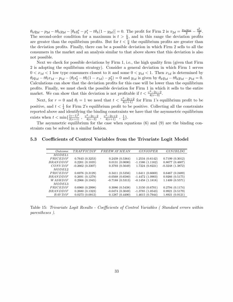
θhq2d − p2d − tθhy2d − [θhq∗1 − p∗1 − tθh(1− y2d)] = 0. The profit for Firm 2 is π2d =p2dy2d2 − q22d
2 .The second-order condition for a maximum is t > υ
8 , and in this range the deviation profitsare greater than the equilibrium profits. But for t < υ
8 the equilibrium profits are greater thanthe deviation profits. Finally, there can be a possible deviation in which Firm 2 sells to all theconsumers in the market and an analysis similar to that above shows that this deviation is alsonot possible.
Next we check for possible deviations by Firm 1, i.e., the high quality firm (given that Firm2 is adopting the equilibrium strategy). Consider a general deviation in which Firm 1 serves0 < x1d < 1 low type consumers closest to it and some 0 < y1d < 1. Then x1d is determined byθlq1d − tθlx1d − p1d − (θls∗2 − tθl(1− x1d)− p∗2) = 0 and y1d is given by θhq1d − tθhy1d − p1d = 0.Calculations can show that the deviation profits for this case will be lower than the equilibriumprofits. Finally, we must check the possible deviation for Firm 1 in which it sells to the entiremarket. We can show that this deviation is not profitable if t < υ2−2υ−2
4(υ−3) .
Next, for r = 0 and θl = 1 we need that t <υ2−2υ+24(υ+1) for Firm 1’s equilibrium profit to be
positive, and t < 14 for Firm 2’s equilibrium profit to be positive. Collecting all the constraints
reported above and identifying the binding constraints we have that the asymmetric equilibrium
exists when t < min{ (υ−1)22(υ+1) ,υ2−2υ−24(υ−3) , υ2−2υ+2
4(υ+1) , 14}.
The asymmetric equilibrium for the case when equations (6) and (9) are the binding con-straints can be solved in a similar fashion.
5.3 Coefficients of Control Variables from the Trivariate Logit Model
Outcome TRAFFICDIF FREEWAYMEAN GINIOPER GINIBLDGMODEL1
PRICEDIF 0.7643 (0.3253) 0.2439 (0.5364) 1.2534 (0.6142) 0.7199 (0.3012)BRANDDIF 0.2201 (0.1035) 0.0131 (0.0690) -1.1586 (1.1162) 0.8677 (0.4607)CONVDIF -0.2662 (0.3307) 0.3793 (0.5649) 1.7224 (0.8221) -0.3248 (1.3872)MODEL2
PRICEDIF 0.6976 (0.3129) 0.3411 (0.5356) 1.6411 (0.6669) 0.6467 (0.2489)BRANDDIF 0.2691 (0.1279) -0.0568 (0.6580) -1.4472 (1.0903) 0.9266 (0.5175)WASHDIF 0.2966 (0.1945) -0.7188 (0.5313) -0.1458 (1.1818) 1.1409 (0.5571)MODEL3
PRICEDIF 0.6960 (0.2998) 0.3086 (0.5438) 1.3150 (0.6701) 0.2794 (0.1174)BRANDDIF 0.2680 (0.1323) -0.0474 (0.3049) -1.3785 (1.0543) 0.9921 (0.5179)
BAYDIF 0.0273 (0.0912) 0.1287 (0.4490) 1.4615 (0.7944) 1.8921 (0.9121)
Table 15: Trivariate Logit Results - Coefficients of Control Variables ( Standard errors withinparentheses ).
33

Outcome TRAFFICDIF FREEWAYMEAN GINIOPER GINIBLDGMODEL4
PRICEDIF 0.7575 (0.3251) 0.2540 (0.5509) 1.2215 (0.6850) 0.6953 (0.2593)HOURSDIF 0.3142 (0.1111) -0.3345 (0.5263) 0.5592 (0.2568) 1.2059 (0.6076)CONV DIF -0.3425 (0.3307) 0.4108 (0.5649) 1.9027 (0.8221) -0.6246 (1.3872)MODEL5
PRICEDIF 0.6754 (0.3149) 0.3528 (0.5702) 1.6492 (0.6499) 0.5637 (0.2394)HOURSDIF 0.2402 (0.1119) -0.1898 (0.5295) 0.7697 (0.4330) 1.0022 (0.5069)WASHDIF 0.2611 (0.1980) -0.6928 (0.5281) -0.2451 (1.4812) 0.9932 (0.3618)MODEL6
PRICEDIF 0.6941 (0.3302) 0.3050 (0.5435) 1.3498 (0.6042) 0.2681 (0.1603)HOURSDIF 0.3059 (0.1504) -0.3582 (0.5788) 0.3379 (0.2374) 0.7755 (0.3435)
BAYDIF -0.0794 (0.4471) 0.2389 (0.6163) 1.4454 (0.7861) 1.5958 (0.8161)
Table 16: Trivariate Logit Results - Coefficients of Control Variables ( Standard errors withinparentheses ).
Outcome TRAFFICDIF FREEWAYMEAN GINIOPER GINIBLDGMODEL7
PRICEDIF 0.8184 (0.3304) 0.2554 (0.5646) 1.3682 (0.6327) 0.8508 (0.3395)NOZDIF 0.3685 (0.2032) 0.0780 (0.4913) 0.9262 (0.4677) 0.8736 (0.4599)
CONV DIF -0.3292 (0.3306) 0.3729 (0.5679) 1.9092 (0.8971) -0.5442 (1.3566)MODEL8
PRICEDIF 0.7307 (0.3182) 0.3627 (0.5518) 1.8209 (0.6584) 0.7135 (0.2373)NOZDIF 0.3332 (0.3026) 0.1478 (0.4895) 1.0230 (0.4805) 0.7735 (0.3374)
WASHDIF 0.2706 (0.1008) -0.7291 (0.5128) -0.2106 (0.8733) 1.0792 (0.5233)MODEL9
PRICEDIF 0.7381 (0.2965) 0.3226 (0.5299) 1.4765 (0.6806) 0.3643 (0.1116)NOZDIF 0.3538 (0.3012) 0.0913 (0.5671) 0.9596 (0.4029) 0.8054 (0.3774)BAYDIF -0.0003 (0.3786) 0.1279 (0.2256) 1.5019 (0.7430) 1.8085 (0.8856)
Table 17: Trivariate Logit Results - Coefficients of Control Variables ( Standard errors withinparentheses ).
Outcome TRAFFICDIF FREEWAYMEAN GINIOPER GINIBLDGMODEL10PRICEDIF 0.8957 (0.3353) 0.1601 (0.6327) 1.2718 (0.6069) 0.8077 (0.3970)PAY DIF 0.7762 (0.3162) -0.5148 (0.5227) 0.2065 (1.2250) 0.5127 (0.2856)
CONV DIF -0.3715 (0.3334) 0.4174 (0.5653) 1.9410 (0.8474) -0.5377 (1.2925)MODEL11PRICEDIF 0.8085 (0.3244) 0.2531 (0.5794) 1.7359 (0.7509) 0.7096 (0.3092)PAY DIF 0.8257 (0.3207) -0.6286 (0.5263) 0.3227 (1.1305) 0.6956 (0.3334)
WASHDIF 0.4319 (0.3044) -0.8217 (0.4518) -0.0839 (1.1957) 1.2426 (0.6063)MODEL12PRICEDIF 0.7951 (0.3338) 0.2434 (0.5689) 1.3984 (0.6657) 0.3232 (0.1173)PAY DIF 0.7500 (0.3122) -0.4819 (0.5185) 0.3862 (1.2359) 0.5248 (0.2637)BAYDIF 0.0379 (0.4001) 0.1153 (0.5544) 1.5503 (0.7405) 1.8534 (0.9678)
Table 18: Trivariate Logit Results - Coefficients of Control Variables ( Standard errors withinparentheses ).
34

Outcome TRAFFICDIF FREEWAYMEAN GINIOPER GINIBLDGMODEL13PRICEDIF 0.7584 (0.3300) 0.3027 (0.5635) 1.2424 (0.6134) 0.5988 (0.2542)FULLDIF 0.1160 (0.4032) -0.6903 (0.6516) -0.0761 (1.6407) 1.8850 (0.9218)CONV DIF -0.3474 (0.3536) 0.6340 (0.6462) 1.9754 (0.9597) -1.0756 (1.3333)MODEL14PRICEDIF 0.6942 (0.3163) 0.4159 (0.5399) 1.5745 (0.7635) 0.4261 (0.2299)FULLDIF -0.0332 (0.3163) -0.4006 (0.5839) 0.7338 (0.4394) 1.4171 (0.7854)WASHDIF 0.2958 (0.2881) -0.7049 (0.5130) -0.1568 (0.9773) 1.1027 (0.5773)MODEL15PRICEDIF 0.6924 (0.3197) 0.3533 (0.5415) 1.3488 (0.6015) 0.2220 (0.1795)FULLDIF -0.0358 (0.3145) -0.6405 (0.6677) -0.0669 (0.6982) 0.6895 (0.2893)BAYDIF 0.0289 (0.0573) 0.4248 (0.6428) 1.5493 (0.7848) 1.5699 (0.7980)
Table 19: Trivariate Logit Results - Coefficients of Control Variables ( Standard errors withinparentheses ).
35
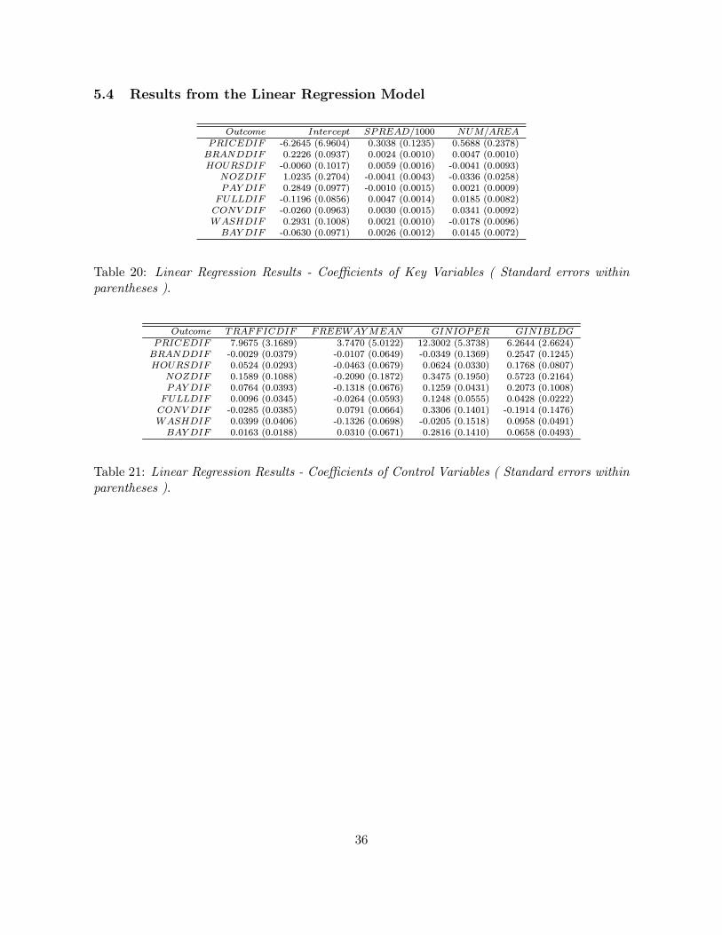
5.4 Results from the Linear Regression Model
Outcome Intercept SPREAD/1000 NUM/AREAPRICEDIF -6.2645 (6.9604) 0.3038 (0.1235) 0.5688 (0.2378)BRANDDIF 0.2226 (0.0937) 0.0024 (0.0010) 0.0047 (0.0010)HOURSDIF -0.0060 (0.1017) 0.0059 (0.0016) -0.0041 (0.0093)
NOZDIF 1.0235 (0.2704) -0.0041 (0.0043) -0.0336 (0.0258)PAY DIF 0.2849 (0.0977) -0.0010 (0.0015) 0.0021 (0.0009)FULLDIF -0.1196 (0.0856) 0.0047 (0.0014) 0.0185 (0.0082)CONV DIF -0.0260 (0.0963) 0.0030 (0.0015) 0.0341 (0.0092)WASHDIF 0.2931 (0.1008) 0.0021 (0.0010) -0.0178 (0.0096)BAY DIF -0.0630 (0.0971) 0.0026 (0.0012) 0.0145 (0.0072)
Table 20: Linear Regression Results - Coefficients of Key Variables ( Standard errors withinparentheses ).
Outcome TRAFFICDIF FREEWAYMEAN GINIOPER GINIBLDGPRICEDIF 7.9675 (3.1689) 3.7470 (5.0122) 12.3002 (5.3738) 6.2644 (2.6624)BRANDDIF -0.0029 (0.0379) -0.0107 (0.0649) -0.0349 (0.1369) 0.2547 (0.1245)HOURSDIF 0.0524 (0.0293) -0.0463 (0.0679) 0.0624 (0.0330) 0.1768 (0.0807)
NOZDIF 0.1589 (0.1088) -0.2090 (0.1872) 0.3475 (0.1950) 0.5723 (0.2164)PAY DIF 0.0764 (0.0393) -0.1318 (0.0676) 0.1259 (0.0431) 0.2073 (0.1008)FULLDIF 0.0096 (0.0345) -0.0264 (0.0593) 0.1248 (0.0555) 0.0428 (0.0222)CONVDIF -0.0285 (0.0385) 0.0791 (0.0664) 0.3306 (0.1401) -0.1914 (0.1476)WASHDIF 0.0399 (0.0406) -0.1326 (0.0698) -0.0205 (0.1518) 0.0958 (0.0491)BAYDIF 0.0163 (0.0188) 0.0310 (0.0671) 0.2816 (0.1410) 0.0658 (0.0493)
Table 21: Linear Regression Results - Coefficients of Control Variables ( Standard errors withinparentheses ).
36