Page 1 of 26

Too Big to Fail: Large Samples and the P-Value Problem

Abstract

The Internet has provided IS researchers with the opportunity to conduct studies with extremely large samples, frequently well over 10,000 observations. There are many advantages to large samples, but researchers using statistical inference must be aware of the p-value problem associated with them. In very large samples, p-values go quickly to zero, and solely relying on p-values can lead the researcher to claim support for results of no practical significance. In a survey of large sample IS research, we found that a significant number of papers rely on a low p-value and the sign of a regression coefficient alone to support their hypotheses. This research commentary recommends a series of actions the researcher can take to mitigate the p-value problem in large samples and illustrates them with an example of over 300,000 camera sales on eBay. We believe that addressing the p-value problem will increase the credibility of large sample IS research as well as provide more insights for readers.

Introduction Advances in technology have brought us the ability to collect, transfer, and store large datasets.

Thanks to this, a growing number of empirical studies published in the information systems and

related fields now rely on very large samples. Some samples include tens of thousands of

observations: For example, Pavlou and Dimoka (2006) use “over 10,000 publicly available

feedback text comments… in eBay”; Overby and Jap (2009) use “108,333 used vehicles offered

in the wholesale automotive market”; Forman, Ghose and Wiesenfeld (2008) “collected data on

… [175,714] reviews from Amazon”; Goldfarb and Lu (2006) report “For our analysis, we have

… 784,882 [portal visits]”, and finally, Ghose and Yao (2011) use “3.7 million records,

encompassing transactions for the Federal Supply Service (FSS) of the U.S. Federal government

in fiscal year 2000.”

Page 2 of 26

With such large samples, some approaching the population itself, conclusions based on

small-sample statistical inferences can be ineffective at best and misleading at worst. In this

paper we try to answer a few important questions that researchers and consumers of large sample

studies should be aware of. These include how do large-sample studies approach statistical

modeling and inference? What are the advantages of large samples and what are the problems of

using small sample inference in this realm?

A key issue with applying small-sample statistical inference to large samples is that even

minuscule effects can become statistically significant. The increased power leads to a dangerous

pitfall as well as to a huge opportunity. The issue is one that statisticians have long been aware

of: “the p-value problem.” Chatfield (1995) comments, “The question is not whether differences

are ‘significant’ (they nearly always are in large samples), but whether they are interesting.

Forget statistical significance, what is the practical significance of the results?” The increased

power of large samples means that researchers can detect smaller, subtler and more complex

effects, but relying on p-values alone can lead to claims of support for hypotheses of little or no

practical significance.

This paper is organized as follows: We start by explaining how and why p-values quickly

approach zero as sample sizes increase, and discuss the potential pitfalls when relying solely on

p-values and coefficient signs in large sample studies. Next, we survey the IS literature for

current practices employed in large sample studies. We examine the extent of the p-value

problem as well as identify practices that take advantage of large samples for improving

inference. We continue by describing practices from other disciplines as well as introducing

Page 3 of 26

methods for mitigating the deflated p-value problem. Finally, we discuss ways to take advantage

of large samples.

The p-value Problem in Large Samples Statistical inference is based on the notion of the null hypothesis. Under the null hypothesis, a

parameter of interest is set to a particular value1, typically zero, which represents the “no effect”

relative to the effect the researcher is testing for. For example, a hypothesis of a positive

regression coefficient requires defining the null hypothesis that the coefficient is 0 for “no effect”

or negative for the “opposite effect.” A non-directional hypothesis requires defining the null

hypothesis that the coefficient is zero. The large sample challenge arises from representing “no

effect” by a particular number (such as zero); when our estimate becomes so precise, even

deviations such as 3E-052 from the null value are identified as statistically significant. More

formally, p-values that are based on consistent estimators have the following limiting behavior

under H0:β = 0:2

lim𝑛→∞

𝑝-value = lim𝑛→∞

𝑃���̂� − 𝛽� < 𝜀� = �0 if β≠01 if β=0

�

In other words, the limiting distribution of the estimator β� has all its mass on the

population parameter 𝛽. Hence, unless the population parameter 𝛽 is exactly equal to the null

value with an infinite number of decimals (in which case the p-value will approach 1), the p-

value will approach 0. Because in real studies the population parameter is typically not a round

1 Or a range of values 2 The result holds for any value k specified in H0: β = 𝑘

Page 4 of 26

figure, a large sample will yield p-values that are near zero. The appendix illustrates this property

for a linear regression coefficient.

A p-value measures the distance between the data and the null hypothesis using an

estimate of the parameter of interest. The distance is typically measured in units of standard

deviations of that estimate (standard errors). For example, tests for a regression coefficient 𝛽1 are

based on the distance of 𝛽1 from zero in units of standard errors. Consistent estimators have

standard errors that shrink as the sample size increases. With a very large sample, the standard

error becomes extremely small, so that even minuscule distances between the estimate and the

null hypothesis become statistically significant. As Tukey (1991) put it, in the context of

comparing groups A and B: “Are the effects of A and B different? They are always different –

for some decimal place.” Cohen (1990) says “A little thought reveals a fact widely understood

among statisticians: The null hypothesis, taken literally (and that’s the only way you can take it

in formal hypothesis testing), is always false in the real world….If it is false, even to a tiny

degree, it must be the case that a large enough sample will produce a significant result and lead

to its rejection. So if the null hypothesis is always false, what’s the big deal about rejecting it?”

We are not suggesting that IS researchers abandon hypothesis testing altogether; after all,

in any given context, there is no guarantee that we always have “a large enough sample” to

produce statistically significant results. The foregoing observations on the null hypothesis are

intended to move our focus from relying solely on statistical significance to consideration of

practical significance and effect size. In other words, with extremely large samples, we should go

beyond rejecting a null hypothesis based on the sign of the coefficient (positive or negative) and

the p-value. Rather, researchers should be cautious in assessing whether the small p-value is just

Page 5 of 26

an artifact of the large sample size, and carefully quantify the magnitude and sensitivity of the

effect. In other words, conclusions based on significance and sign alone, claiming that the null

hypothesis is rejected, are meaningless unless interpreted in light of the actual magnitude of the

effect size.3

In what follows, we conduct a brief survey of how other fields have tried or are trying to

deal with this problem. We then examine the current practice in our own field, and propose

actionable recommendations for IS researchers, illustrating them using a large sample of camera

sales on eBay.

The leap from statistical significance to managerial and policy implications is

therefore not warranted.

The p-Value Problem in Other Fields Statisticians have long been divided in their views on using p-values, regardless of sample size.

One stream in statistics rejects the use of hypothesis testing altogether and advocates moving to

estimation, where one reports point estimates and confidence intervals (Hubbard and Armstrong

2006). Those who are not opposed to hypothesis testing stress the need to focus on practical

significance rather than statistical significance. When more complex models are constructed,

marginal analysis can be used for identifying and illustrating practical magnitude.

In empirical economics, a common practice is to report confidence intervals, or,

depending on the context, to be more conservative and report only one of its bounds (Cannon

and Cipriani 2006, Disdier and Head 2008, Goolsbee and Guryan 2006). Whereas the p-value

3 With a sufficiently large sample tests of model assumptions will tend to indicate a violation even for very small deviations. Common tests for heteroscedasticity include the Breusch-Pagan and White tests. The Durbin-Watson is often used to test for serial correlation. Pairwise correlations are examined for checking multicollinearity. In these tests, the null hypothesis states that the assumption is met (no violation).. A researcher relying only on statistical significance will tend to perform various model and data modifications to address the assumption violations that may be unwarranted.

Page 6 of 26

only describes the probability that the null hypothesis can be rejected given a true effect, the

confidence interval (CI) gives a range for the actual magnitude of the parameter of interest. As

the sample size increases, a typical CI will become narrower. In other words, while the

information that p-values convey does not scale up to large samples, the information contained in

confidence intervals does, as the range estimate becomes more precise. This property means that

even if the researcher is unsure whether the sample is too large for using p-values, relying on a

CI is always safe.

Some econometricians have a different suggestion about ever-decreasing p-values: adjust

the threshold p-value downward as the sample size grows (Greene 2002, Leamer 1978). The

argument is that instead of claiming significance when p<5%, for instance, with very large

samples the threshold should be 1%, 0.1%, or even smaller. However, to our knowledge, this

approach has not been used and there have been no proposed rules-of-thumb in terms of how

such adjustments should be made.

Large sample studies in IS: A survey of current practice At a recent seminar at one of our universities, a researcher presented a paper with nearly 10,000

observations and discussed the regression results solely on the basis of statistical significance;

there was no mention of effect sizes or caveats relating to the sample size. This approach appears

to be common practice. We reviewed articles in MIS Quarterly, Information Systems Research

and Management Science between 2004-2010 along with abstracts from the Workshop on

Information Systems and Economics and symposia on Statistical Challenges in Electronic

Commerce Research to see to what extent IS researchers recognized the issues in analyzing large

Page 7 of 26

samples.4

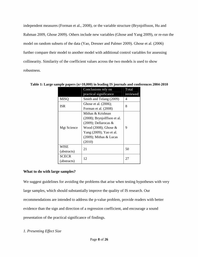
In Table 1 we find that about half of the recent papers with large samples rely almost

exclusively on low p-values and the sign of the coefficient. More specifically, this percentage is

50% for recent papers with sample sizes over 10,000 in the two leading IS journals, MIS

Quarterly and Information Systems Research; and 57% of large sample papers in two IS

conferences (WISE and SCECR). It is interesting to note that compared to ISR and MISQ, all

reviewed papers in Management Science – a more general publication – report practical

significance.

Our overall conclusion is that information systems research that is based on large

samples might be over-relying on p-values to interpret findings.

In reviewing the literature, we found only a few mentions of the large sample issue and

its effect on p-values; we also saw little recognition that the authors’ low p-values might be an

artifact of their large sample sizes. Authors who recognized the “large sample, small p-values”

issue addressed it by one of the following approaches: reducing the significance level threshold5

Gefen and Carmel

2008

(which does not really help), by re-computing the p-value for a small sample (

), or by focusing on practical significance and commenting about the uselessness of

statistical significance (Mithas and Lucas 2010).

In some cases, authors report confidence intervals (Dellarocas and Wood 2008, Overby

and Jap 2009), and marginal effects charts appear in a few papers (Moon and Sproull 2008).

Authors of several of the papers conducted robustness/sensitivity analysis, modifying the 4 Only abstracts are available for the two conference series so we have more confidence in the results for the two journals. 5 “The significance level deemed appropriate was the smallest value reported by the SPSS package for the analysis in question. For large-scale analysis this was p <0.0000, and for analysis with hundreds of variables this was p<0.000.” (Jones et al., 2004); “because we have a very large number of observations, we adopt a conservative approach and report results as statistically significant only when they are significant at the 5% level or better.” (Forman et al., 2008)

Page 8 of 26

independent measures (Forman et al., 2008), or the variable structure (Brynjolfsson, Hu and

Rahman 2009, Ghose 2009). Others include new variables (Ghose and Yang 2009), or re-run the

model on random subsets of the data (Yao, Dresner and Palmer 2009). Ghose et al. (2006)

further compare their model to another model with additional control variables for assessing

collinearity. Similarity of the coefficient values across the two models is used to show

robustness.

Table 1: Large sample papers (n>10,000) in leading IS journals and conferences 2004-2010

Conclusions rely on practical significance

Total reviewed

MISQ Smith and Telang (2009) 4

ISR Ghose et al. (2006); Forman et al. (2008)

8

Mgt Science

Mithas & Krishnan (2008); Brynjolffson et al. (2009); Dellarocas & Wood (2008); Ghose & Yang (2009); Yao et al. (2009); Mithas & Lucas (2010)

9

WISE (abstracts) 21 50

SCECR (abstracts)

12 27

What to do with large samples? We suggest guidelines for avoiding the problems that arise when testing hypotheses with very

large samples, which should substantially improve the quality of IS research. Our

recommendations are intended to address the p-value problem, provide readers with better

evidence than the sign and direction of a regression coefficient, and encourage a sound

presentation of the practical significance of findings.

1. Presenting Effect Size

Page 9 of 26

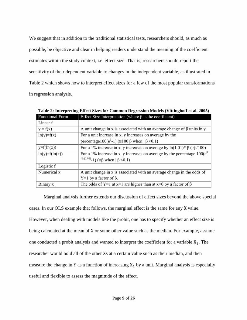
We suggest that in addition to the traditional statistical tests, researchers should, as much as

possible, be objective and clear in helping readers understand the meaning of the coefficient

estimates within the study context, i.e. effect size. That is, researchers should report the

sensitivity of their dependent variable to changes in the independent variable, as illustrated in

Table 2 which shows how to interpret effect sizes for a few of the most popular transformations

in regression analysis.

Table 2: Interpreting Effect Sizes for Common Regression Models (Vittinghoff et al. 2005) Functional Form Effect Size Interpretation (where β is the coefficient) Linear f y = f(x) A unit change in x is associated with an average change of β units in y ln(y)=f(x) For a unit increase in x, y increases on average by the

percentage100(eβ-1) (≅100 β when | β|<0.1) y=f(ln(x)) For a 1% increase in x, y increases on average by ln(1.01)* β (≅β/100) ln(y)=f(ln(x)) For a 1% increase in x, y increases on average by the percentage 100(eβ

*ln(1.01)-1) (≅β when | β|<0.1) Logistic f Numerical x A unit change in x is associated with an average change in the odds of

Y=1 by a factor of β. Binary x The odds of Y=1 at x=1 are higher than at x=0 by a factor of β

Marginal analysis further extends our discussion of effect sizes beyond the above special

cases. In our OLS example that follows, the marginal effect is the same for any X value.

However, when dealing with models like the probit, one has to specify whether an effect size is

being calculated at the mean of X or some other value such as the median. For example, assume

one conducted a probit analysis and wanted to interpret the coefficient for a variable X1. The

researcher would hold all of the other Xs at a certain value such as their median, and then

measure the change in Y as a function of increasing X1 by a unit. Marginal analysis is especially

useful and flexible to assess the magnitude of the effect.

Page 10 of 26

For nonlinear models, which are quite common in IS research, marginal analysis is a

more robust way – and sometimes the only way — to interpret effect size, compared to looking

at the p-value or magnitude of the coefficient. As an example, if we have X1 and X12 as the

explanatory variables for Y, it is incorrect to directly interpret the marginal effect of X1 solely

based on its coefficients, because we cannot hold X12 constant and at the same time increase X1

by one unit.

Reporting the effect size does not have to be done strictly in terms of 1 unit / percentage

change in X leading to a certain unit / percentage change in Y. In fact for the general reader, it

would be especially useful if the researcher can translate effects into something that is easy to

understand. Suppose a researcher finds that eating an apple a day reduces the chance of falling ill

from 3% to 2%. One could say “each additional apple consumed per day reduces the chances of

going to the doctor on average by 33% ,” and that “including an apple a day in your diet is likely

to reduce your risk of becoming ill from 3% to 2%.” This interpretation is much more

informative because (1) it shows the point of comparison (X=0, no apple); (2) the traditional

sense of the effect size ((3%-2%)/3%=33%); and (3) the relative magnitude of the effect size

(going from 3% to 2%).

This hypothetical example also illustrates that the practical significance of a research

finding depends on the domain and the point of view of the reader. A change in the chance of

falling ill from 3% to 2% may be very significant for policy makers when they look at the whole

population, and it may be also significant for someone who is highly health-conscious, but not so

much for someone who is not that concerned about health. Such interpretations are not only more

Page 11 of 26

straightforward, but they also facilitate the transfer of research results from researchers to the

general readership.

2. Reporting Confidence Intervals We recommend that IS researchers working with large samples report effect sizes using

confidence intervals, an approach often used in empirical economics research as discussed

previously. There are a number of major benefits to reporting confidence intervals over p-values

and coefficient signs. First, confidence intervals address the problem that motivated this paper:

the tendency of large-sample IS research to rely on low p-values and the direction of a regression

coefficient to support the researcher’s propositions. Second, when researchers report the

confidence intervals for a particular variable across different studies, it becomes much easier to

conduct meta-analysis, synthesize prior studies, and help advance scientific knowledge of the

relevant IS field. This is particularly true when the CI is for elasticities (that is, the percentage

change in Y for each 1% change in X). An example can be found in de Leeuw (1971) from the

labor economics literature.

When the researcher has a particular parameter value of interest k, such as based on prior

research, then a confidence interval for the coefficient will give an indication of the closeness of

the coefficient not only to k but also to other values in the vicinity of k6. Because a large sample

results in tighter confidence interval, the CI’s thresholds are especially informative of the

(unknown) parameter’s magnitude and range.

6 Alternatively, the researcher may use a series of values for 𝑘 (𝑘1, 𝑘2, 𝑘3, … ), and sequentially test hypotheses 𝛽 = 𝑘1; 𝛽 = 𝑘2; …. This is akin to a series of sensitivity tests around 𝑘, and will yield similar results as the confidence interval approach. We thank an anonymous reviewer for this insight.

Page 12 of 26

Last but not least, empirical IS researchers tend to conduct multiple robustness checks for

their models by comparing multiple model specifications. With CIs, one can go beyond the

argument that “results are qualitatively similar”, and quantitatively compare the range of

estimates. Examples of the use of a CI or one of its bounds can be found in many papers in

different empirical fields (Black and Strahan 2002, Goolsbee 2000, Goolsbee and Guryan 2006,

Iglesias and Riboud 1988, Vissing-Jørgensen 2002).

We advocate using the most conservative bound of the confidence interval and reporting

that the researchers are, for example, 95% confident that the independent variable has the

calculated impact on the dependent variable. This kind of statement is easy for the reader to

interpret and corresponds to the frequent use across a variety of fields of the probability of a

Type I error of 5% without falling into the p-value pitfall.

3. Using Charts Given the importance of statistical inference in IS research, we present an approach that helps

avoid the p-value problem that arises in large sample studies, while maintaining the framework

that researchers are familiar with. We build on a few intuitive notions: First, drawing a smaller

sample will yield “familiar” significance levels. Second, drawing multiple samples gives

additional information about variability in those results. Third, samples of increasing size will

display the p-value deflation problem. We integrate these notions into four charts:

A Confidence Interval (CI) Chart displays the confidence interval as a function of the

sample size, ranging from very small to the maximal large sample size itself. This plot

emphasizes the magnitude of the coefficient and its shrinking standard error.

Page 13 of 26

The Coefficient/p-value/sample-size (CPS) Chart displays curves of the coefficient of

interest and its associated p-value for different samples sizes, ranging from very small to the

maximal large sample size itself. This chart is based on repeatedly drawing samples of increasing

sizes, re-running the statistical model on each sample, computing the coefficient and p-values of

interest and plotting them on a chart. An algorithm for generating this chart is given in Table 3

(Stata code is available online at http://goo.gl/hfNj4).

A 1% Significance Threshold Chart that shows the sample size at which each variable’s

coefficient becomes significant at the 1% level. It can be used to determine subsample sizes for

checking robustness.

The Monte-Carlo CPS Chart expands the CPS chart by drawing multiple samples from

each sample size. While this chart can be more computationally intensive, it gives the added

information about the distribution of the coefficients and the p-values as the sample size

increases (Stata code is available online at http://goo.gl/vBvJO).

Table 3: Algorithm for generating CPS chart For a sample of size n, and a CPS chart based on k increasing sample sizes:

1. Choose the minimum sample size n0 that is reasonable for fitting the model; 2. Randomly draw a sample of size n0 from the large dataset; 3. Fit the model of interest to this sample, and retain the estimated coefficients, their standard errors,

and the p-values; 4. Increase the last sample size by adding round(n/k) more observations, drawn randomly from the

remaining dataset; 5. Repeat steps (3)-(4) until the full original dataset is used; 6. Finally, create a line plot of the coefficients vs. the sample size (on the x-axis), and in another

panel the p-value(s) vs. the sample size.

It should be noted, however, that producing these charts can be computationally

intensive, so they are most appropriate for models that are straightforward and easy to estimate.

We illustrate some of these proposals using a real dataset from eBay auctions.

Page 14 of 26

Example: Camera Sales on eBay To illustrate the p-value issue that arises in large samples, and the different proposed solutions

(including our CPS and Monte Carlo CPS charts), we use a large sample (n=341,136) of eBay

auctions for digital cameras between August 2007 and January 2008. Summary statistics for the

main variables of interest are in Table 4.

For illustration purposes, we draw on a simple model from earlier studies of auction data

such as the one by Lucking-Reiley et al. (2007)7

.

0 1 2 3

4 5

ln *ln( ) * *ln( ) ( ) (controls)

Price minimumBid reserve sellerFeedbackDuration

β β β ββ β ε

= + + ++ + +

Suppose we have the following four hypotheses regarding price determinants:

H1: Higher minimum bids lead to higher final prices (𝛽1>0) H2: Auctions with reserve price will sell for higher prices (𝛽2>0) H3: Duration affects price (𝛽4≠0) H4: The higher the seller feedback, the higher the price (𝛽3>0)

Table 4: Variable descriptions and summary statistics

Variables Descriptions Mean Standard Deviation minimumBid Minimum bid of the auction 40.9 79 Reserve 1 if seller set a reserve price for

the auction; 0 otherwise 0.035 0.183

sellerFeedback Sellers’ feedback score at time of listing

44074.8 93126.7

Duration Duration of auctions in days 4.12 2.6 Control variables: dummies for camera type, brand, condition, and product lines.

We start by estimating the regression equation using the full sample (n=341,136). Results

are shown in Table 5. The approach of considering only the coefficient sign and the significance

7 This model is for illustration purpose only. All hypotheses and tests are conditional on the fact that the auction is actually successful – i.e. the product is actually sold.

Page 15 of 26

level would lead to the rejection of all four hypotheses, which is not necessarily warranted given

the magnitude of the coefficients. Of course, whether a coefficient magnitude is practically

significant depends on the context and on the stakeholder (e.g., for a seller interested in a single

auction, or the auction house interested in large volumes of auctions).

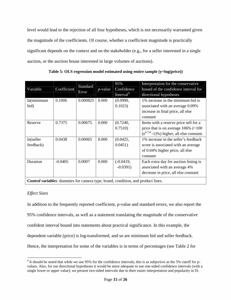
Table 5: OLS regression model estimated using entire sample (y=log(price))

Effect Sizes In addition to the frequently reported coefficient, p-value and standard errors, we also report the

95% confidence intervals, as well as a statement translating the magnitude of the conservative

confident interval bound into statements about practical significance. In this example, the

dependent variable (price) is log-transformed, and so are minimum bid and seller feedback.

Hence, the interpretation for some of the variables is in terms of percentages (see Table 2 for

8 It should be noted that while we use 95% for the confidence intervals, this is as subjective as the 5% cutoff for p-values. Also, for our directional hypotheses it would be more adequate to use one-sided confidence intervals (with a single lower or upper value); we present two-sided intervals due to their easier interpretation and popularity in IS.

Variable Coefficient Standard Error

p-value 95% Confidence Interval8

Interpretation for the conservative bound of the confidence interval for directional hypotheses

ln(minimum bid)

0.1006 0.000825 0.000 (0.0990, 0.1023)

1% increase in the minimum bid is associated with an average 0.09% increase in final price, all else constant

Reserve 0.7375 0.00675 0.000 (0.7240, 0.7510)

Items with a reserve price sell for a price that is on average 106% (=100 (e0.724 -1)%) higher, all else constant.

ln(seller feedback)

0.0438 0.00065 0.000 (0.0425, 0.0451)

1% increase in the seller’s feedback score is associated with an average of 0.04% higher price, all else constant

Duration -0.0405 0.0007 0.000 (-0.0419, -0.0391)

Each extra day for auction listing is associated with an average 4% decrease in price, all else constant

Control variables: dummies for camera type, brand, condition, and product lines.

Page 16 of 26

interpreting coefficient magnitudes in linear and logistic regression with various

transformations).

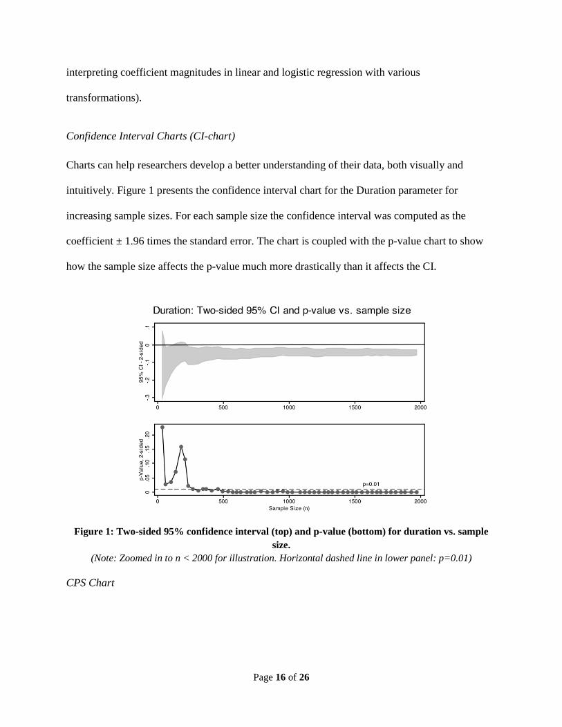
Confidence Interval Charts (CI-chart) Charts can help researchers develop a better understanding of their data, both visually and

intuitively. Figure 1 presents the confidence interval chart for the Duration parameter for

increasing sample sizes. For each sample size the confidence interval was computed as the

coefficient ± 1.96 times the standard error. The chart is coupled with the p-value chart to show

how the sample size affects the p-value much more drastically than it affects the CI.

Figure 1: Two-sided 95% confidence interval (top) and p-value (bottom) for duration vs. sample

size. (Note: Zoomed in to n < 2000 for illustration. Horizontal dashed line in lower panel: p=0.01)

CPS Chart

Page 17 of 26

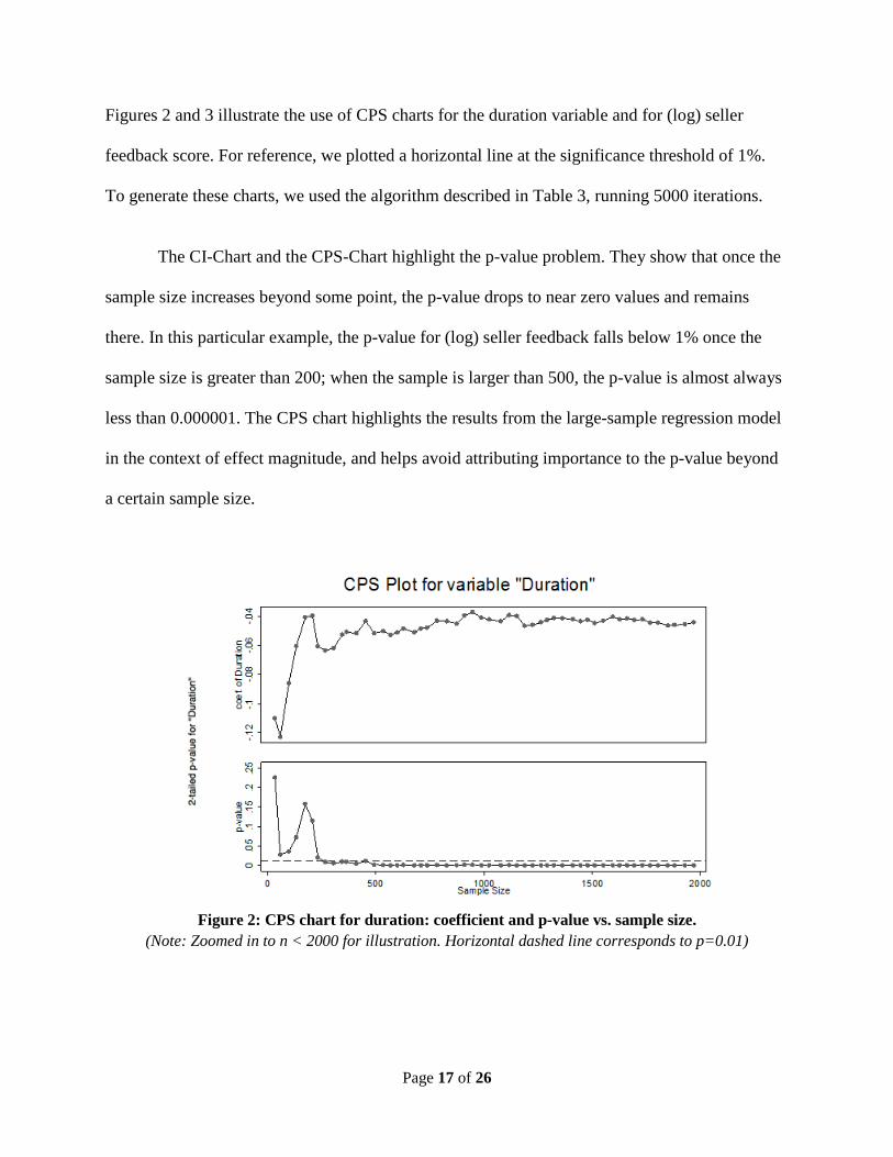
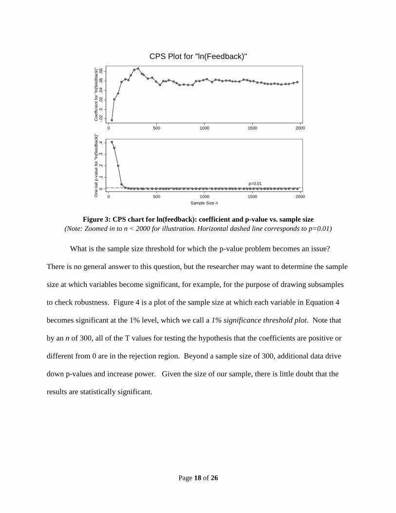
Figures 2 and 3 illustrate the use of CPS charts for the duration variable and for (log) seller

feedback score. For reference, we plotted a horizontal line at the significance threshold of 1%.

To generate these charts, we used the algorithm described in Table 3, running 5000 iterations.

The CI-Chart and the CPS-Chart highlight the p-value problem. They show that once the

sample size increases beyond some point, the p-value drops to near zero values and remains

there. In this particular example, the p-value for (log) seller feedback falls below 1% once the

sample size is greater than 200; when the sample is larger than 500, the p-value is almost always

less than 0.000001. The CPS chart highlights the results from the large-sample regression model

in the context of effect magnitude, and helps avoid attributing importance to the p-value beyond

a certain sample size.

Figure 2: CPS chart for duration: coefficient and p-value vs. sample size.

(Note: Zoomed in to n < 2000 for illustration. Horizontal dashed line corresponds to p=0.01)

Page 18 of 26

Figure 3: CPS chart for ln(feedback): coefficient and p-value vs. sample size

(Note: Zoomed in to n < 2000 for illustration. Horizontal dashed line corresponds to p=0.01)

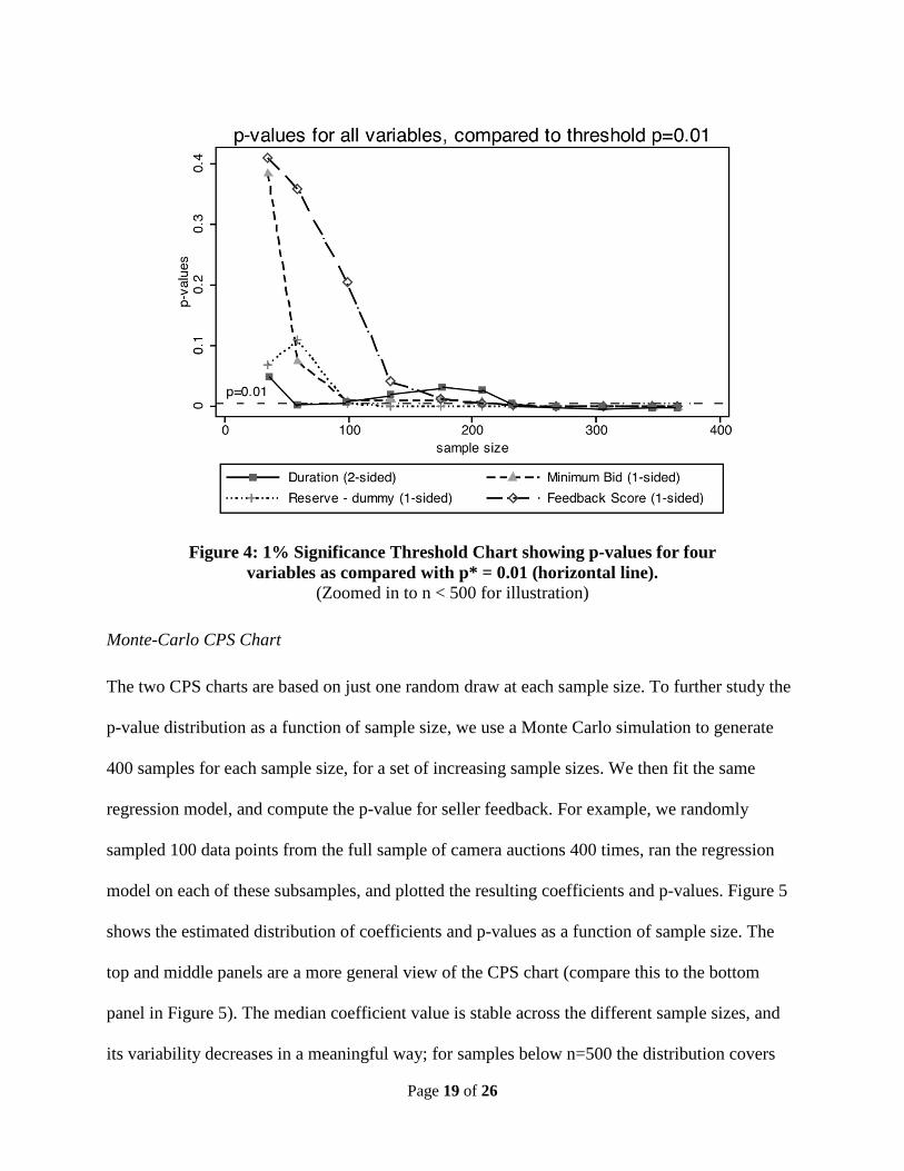
What is the sample size threshold for which the p-value problem becomes an issue?

There is no general answer to this question, but the researcher may want to determine the sample

size at which variables become significant, for example, for the purpose of drawing subsamples

to check robustness. Figure 4 is a plot of the sample size at which each variable in Equation 4

becomes significant at the 1% level, which we call a 1% significance threshold plot. Note that

by an n of 300, all of the T values for testing the hypothesis that the coefficients are positive or

different from 0 are in the rejection region. Beyond a sample size of 300, additional data drive

down p-values and increase power. Given the size of our sample, there is little doubt that the

results are statistically significant.

-.02

0.0

2.0

4.0

6.0

8C

oeffi

cien

t for

"ln(

feed

back

)"

0 500 1000 1500 2000

p=0.01

0.1

.2.3

.4O

ne-ta

il p-

valu

e fo

r "ln

(feed

back

)"

0 500 1000 1500 2000Sample Size n

CPS Plot for "ln(Feedback)"

Page 19 of 26

Figure 4: 1% Significance Threshold Chart showing p-values for four

variables as compared with p* = 0.01 (horizontal line). (Zoomed in to n < 500 for illustration)

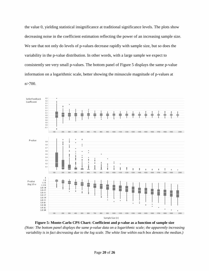
Monte-Carlo CPS Chart The two CPS charts are based on just one random draw at each sample size. To further study the

p-value distribution as a function of sample size, we use a Monte Carlo simulation to generate

400 samples for each sample size, for a set of increasing sample sizes. We then fit the same

regression model, and compute the p-value for seller feedback. For example, we randomly

sampled 100 data points from the full sample of camera auctions 400 times, ran the regression

model on each of these subsamples, and plotted the resulting coefficients and p-values. Figure 5

shows the estimated distribution of coefficients and p-values as a function of sample size. The

top and middle panels are a more general view of the CPS chart (compare this to the bottom

panel in Figure 5). The median coefficient value is stable across the different sample sizes, and

its variability decreases in a meaningful way; for samples below n=500 the distribution covers

Page 20 of 26

the value 0, yielding statistical insignificance at traditional significance levels. The plots show

decreasing noise in the coefficient estimation reflecting the power of an increasing sample size.

We see that not only do levels of p-values decrease rapidly with sample size, but so does the

variability in the p-value distribution. In other words, with a large sample we expect to

consistently see very small p-values. The bottom panel of Figure 5 displays the same p-value

information on a logarithmic scale, better showing the minuscule magnitude of p-values at

n>700.

Figure 5: Monte-Carlo CPS Chart: Coefficient and p-value as a function of sample size

(Note: The bottom panel displays the same p-value data on a logarithmic scale; the apparently increasing variability is in fact decreasing due to the log scale. The white line within each box denotes the median.)

Page 21 of 26

Taking Advantage of Large Samples Large samples provide opportunities to conduct more powerful data analysis and inference

compared to small samples. In this section, we highlight some ways of exploiting large samples,

with reference to some published papers that already do so.

One major opportunity with large samples is the detection and quantification of small or

complex effects. Examples include non-linear relationships, such as higher-order polynomials

and interaction terms (Asvanund et al. 2004, Forman et al. 2008, Ghose and Yang 2009). In such

cases the interpretation of effects must take into account the additional coefficients (e.g., X2 or

X1*X2). Moreover, with a large sample, interactions that involve a categorical variable can be

studied by splitting the data into the separate categories and fitting separate models (Asvanund et

al. 2004, Forman et al. 2008, Gefen and Carmel 2008, Ghose 2009, Gordon, Loeb and Sohail

2010, Li and Hitt 2008, Mithas and Lucas 2010, Overby and Jap 2009, Yao et al. 2009). In

general, a large sample often provides sufficient data for conducting analyses on subsamples of

interest while maintaining sufficient power in each subsample. For example, a researcher might

analyze subsamples by geographic area or by product type, with special interest in particular

categories.

A large sample also enables the researcher to incorporate many control variables into the

model without worrying about power loss (Forman et al. 2008, Ghose 2009, Mithas and Lucas

2010), thereby reducing concerns for alternative explanations and strengthen the main arguments

if results remain consistent.

If a researcher would like to validate the predictive power of her causal model, it is easier

to do so with a large sample (Shmueli 2010, Shmueli and Koppius 2011). The researcher would

Page 22 of 26

remove a random portion of the sample before analysis begins, estimate the causal model (on the

reduced sample), and then generate predictions of the dependent variable for the excluded

“holdout set” of observations. The closeness of the predictions to the actual dependent variable

values gives an indication of the predictive power of her model.

Some effects are so rare that they are encountered only with a very large sample. This is

one of the main uses of large samples in industry in applications such as fraud detection. While

research tends to focus on the “average behavior”, with large samples we can expand scientific

endeavors into the “rare events” realm, which are often important. One example is Dellarocas

and Wood (2008). In addition to their main analysis, the authors look more carefully at negative

and neutral ratings on eBay, which account for a small percentage of ratings on the site.

Conclusions The purpose of this commentary is to highlight a significant challenge in IS research that may

reduce the credibility of our findings. Larger samples provide great opportunities for empirical

researchers, but also create potential problems in interpreting statistical significance. The

challenge is to take advantage of these large samples without falling victim to deflating p-values.

In particular we recommend that IS researchers modeling large samples should not simply rely

on the direction of a regression coefficient and a low p-value to support their hypotheses.

Instead, we suggest several approaches to the p-value problem: reporting effect sizes and

confidence intervals, reporting conservatively using, for example, the minimum point of the

confidence interval, and using various plots for interpreting the data along with Monte Carlo

simulations. As IS researchers increasingly gain access to large datasets, we hope that this

Page 23 of 26

commentary will stimulate an ongoing discussion on the advantages and challenges of

conducting large sample research in information systems.

Appendix: Why the p-Value Approaches 0 for Large Samples Traditionally, empirical research papers in IS explicitly discuss and elaborate on what a statistician would call the alternative hypothesis, for example, that females use smart phones for texting more than males or that a higher starting bid in an online auction is associated with a higher final price for the goods being auctioned, implicitly implying that the null hypothesis is the “opposite” scenario. Underlying all statistical testing is the null hypothesis which always includes the case of “no effect,” for example, that there are no differences between groups or that there is no association among variables.

The null hypothesis either contains only the non-directional “no effect” scenario or it contains both the “no effect” scenario and the “opposite” directional scenario. The researcher hypothesizing that a coefficient in a regression equation is positive is trying to reject the null hypothesis that the coefficient is 0 or negative, i.e., rejecting the no effect and negative coefficient scenarios. When a researcher reports that the coefficient of the regression equation is positive and statistically significant at the .05 level, there is only a 5% chance that she would have observed this result or one more extreme (i.e., a larger positive coefficient) if in fact the coefficient is 0 or negative.

Consider a researcher who conducts an online survey of college students to test the alternative hypothesis that female students use their smart phones for texting more than male students. The implied null hypothesis is that either there is no gender effect or that male students use their smart phones for texting more than female students. The researcher’s survey displays a line on the respondent’s computer anchored by 0% and 100% on either end, and asks the respondent to click at the percentage of their smart phone use that is for texting. If male and females actually text the same amount, the first problem is accurately measuring the responses from the continuous line where the respondents click on their responses. As Tukey (1991) put it: “Are the effects of A (females) and B (males) different? They are always different---for some decimal place.” Cohen (1990) says “A little thought reveals a fact widely understood among statisticians: The null hypothesis, taken literally (and that’s the only way you can take it in formal hypothesis testing), is always false in the real world….If it is false, even to a tiny degree, it must be the case that a large enough sample will produce a significant result and lead to its rejection. So if the null hypothesis is always false, what’s the big deal about rejecting it?” We are not suggesting that IS researchers abandon hypothesis testing; these observations on the null hypothesis are intended to move our focus from relying solely on statistical significance to consideration of practical significance and effect size.

Large samples are advantageous because of the statistical power that they provide. Yet researchers should also realize that a by-product of increasing the sample size is that the p-value itself will easily go to zero. The p-value for testing a non-directional hypothesis regarding a linear regression coefficient is calculated by: [1] -value 2*(1 ( , ))p df T= − Φ

where Φ is the cumulative student’s t-distribution, df is the residual degrees of freedom, and T is the

absolute value of the observed t-statistic9

βσ

β

ˆˆ0ˆ −

=T, given by .

This T statistic is an increasing function of the sample size n, because the standard error in the denominator decreases in n. In the case of a single independent variable, it is straightforward to see the effect of the sample size on the standard error:

9 Source: Buis, M. L. (2007). Stata tip 53: Where did my p-values go? Stata Journal, 7(4), 584-586.

Page 24 of 26

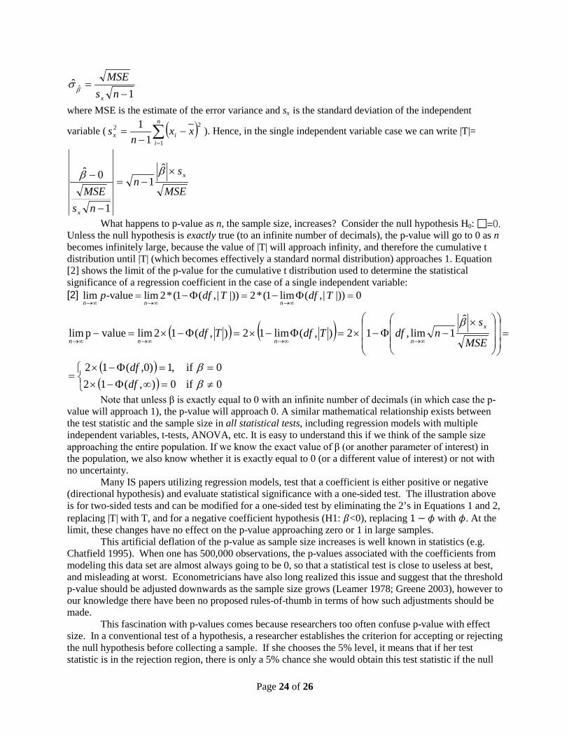
1ˆ ˆ

−=

nsMSE

xβ

σ

where MSE is the estimate of the error variance and sx is the standard deviation of the independent

variable ( ( )∑=

−−

=n

iix xx

ns

1

22

11 ). Hence, in the single independent variable case we can write |T|=

MSE

sn

nsMSE

x

x

×−=

−

− ββ ˆ1

1

0ˆ

What happens to p-value as n, the sample size, increases? Consider the null hypothesis H0: =0. Unless the null hypothesis is exactly true (to an infinite number of decimals), the p-value will go to 0 as n becomes infinitely large, because the value of |T| will approach infinity, and therefore the cumulative t distribution until |T| (which becomes effectively a standard normal distribution) approaches 1. Equation [2] shows the limit of the p-value for the cumulative t distribution used to determine the statistical significance of a regression coefficient in the case of a single independent variable: [2] lim -value lim 2*(1 ( ,| |)) 2*(1 lim ( ,| |)) 0

n n np df T df T

→∞ →∞ →∞= − Φ = − Φ =

( ) ( )( )( )

≠=∞Φ−×==Φ−×

=

=

×−Φ−×=Φ−×=Φ−×=−

∞→∞→∞→∞→

0 if0),(120 if,1)0,(12

ˆ1lim,12),(lim12),(12limvalueplim

ββ

β

dfdf

MSE

sndfTdfTdf

x

nnnn

Note that unless β is exactly equal to 0 with an infinite number of decimals (in which case the p-value will approach 1), the p-value will approach 0. A similar mathematical relationship exists between the test statistic and the sample size in all statistical tests, including regression models with multiple independent variables, t-tests, ANOVA, etc. It is easy to understand this if we think of the sample size approaching the entire population. If we know the exact value of β (or another parameter of interest) in the population, we also know whether it is exactly equal to 0 (or a different value of interest) or not with no uncertainty.

Many IS papers utilizing regression models, test that a coefficient is either positive or negative (directional hypothesis) and evaluate statistical significance with a one-sided test. The illustration above is for two-sided tests and can be modified for a one-sided test by eliminating the 2’s in Equations 1 and 2, replacing |T| with T, and for a negative coefficient hypothesis (H1: 𝛽<0), replacing 1 − 𝜙 with 𝜙. At the limit, these changes have no effect on the p-value approaching zero or 1 in large samples.

This artificial deflation of the p-value as sample size increases is well known in statistics (e.g. Chatfield 1995). When one has 500,000 observations, the p-values associated with the coefficients from modeling this data set are almost always going to be 0, so that a statistical test is close to useless at best, and misleading at worst. Econometricians have also long realized this issue and suggest that the threshold p-value should be adjusted downwards as the sample size grows (Leamer 1978; Greene 2003), however to our knowledge there have been no proposed rules-of-thumb in terms of how such adjustments should be made.

This fascination with p-values comes because researchers too often confuse p-value with effect size. In a conventional test of a hypothesis, a researcher establishes the criterion for accepting or rejecting the null hypothesis before collecting a sample. If she chooses the 5% level, it means that if her test statistic is in the rejection region, there is only a 5% chance she would obtain this test statistic if the null

Page 25 of 26

hypothesis is true. If, instead, she chose the 1% level and the test statistic is in the rejection region, then there is only a 1% chance she would get this result if the null hypothesis is true. The p-value indicates the probability that one would observe the test statistic (or a more extreme value) given the null hypothesis is true. The p-value says nothing about the strength of the effect under investigation. A p-value<.001 does not imply a stronger relationship between variables than a p-value<.01.

As an example, Thompson (1989) presents a table of results with fixed effect sizes showing increasing levels of statistical significance as the sample size increases. The level of statistical significance increases, but the strength of the relationship in the table remains constant. The result becomes statistically significant somewhere between 13 and 23 observations in the sample, but the effect size is fixed.

Researchers in many fields seem to regard a test statistic that allows them to reject the null hypothesis at the 5% level as magical proof of the relationship they believe exists between independent and dependent variables. A focus on a particular level of significance has led to suggestions that we have become so obsessed with 5% that we have forgotten to look at the practical significance of our findings (Carver 1978, Sawyer and Peter 1983, Ziliak and McCloskey 2008).

References

Asvanund, A., K. Clay, R. Krishnan, M.D. Smith. 2004. An empirical analysis of network externalities in peer-to-peer music-sharing networks. Information Systems Research. 15 155-174.

Black, S.E., P.E. Strahan. 2002. Entrepreneurship and bank credit availability. The Journal of Finance. 57(6) 2807-2833.

Brynjolfsson, E., Y.J. Hu, M.S. Rahman. 2009. Battle of the retail channels: How product selection and geography drive cross-channel competition. Management Science. 55(11) 1755-1765.

Cannon, E., G.P. Cipriani. 2006. Euro-illusion: A natural experiment. Journal of Money Credit and Banking. 38(5) 1391.

Carver, R.P. 1978. The case against statistical significance testing. Harvard Educational Review. 48(3) 378-399.

Chatfield, C. 1995. Problem solving: A statistician's guide. Chapman & Hall/CRC. Cohen, J. 1990. Things i have learned (so far). American Psychologist. 45(12) 1304-1312. de Leeuw, F. 1971. The demand for housing: A review of cross-section evidence. Review of Economics &

Statistics. 53(1) 1. Dellarocas, C., C.A. Wood. 2008. The sound of silence in online feedback: Estimating trading risks in the

presence of reporting bias. Management Science. 54(3) 460-476. Disdier, A., K. Head. 2008. The puzzling persistence of the distance effect on bilateral trade. Rev. Econ.

Statist. 90(1) 37-48. Forman, C., A. Ghose, B. Wiesenfeld. 2008. Examining the relationship between reviews and sales: The

role of reviewer identity disclosure in electronic markets. Information Systems Research. 19(3) 291-313.

Gefen, D., E. Carmel. 2008. Is the world really flat? A look at offshoring at an online programming marketplace. MIS Quarterly. 32(2) 367-384.

Ghose, A. 2009. Internet exchanges for used goods: An empirical analysis of trade patterns and adverse selection 1. MIS Quarterly. 33(2) 263-292.

Ghose, A., M. Smith, R. Telang. 2006. Internet exchanges for used books: An empirical analysis of product cannibalization and welfare impact. Information Systems Research. 17(1) 3.

Ghose, A., Y. Yao. 2011. Using Transaction Prices to Re-Examine Price Dispersion in Electronic Markets. Information Systems Research 22(2) 1-17.

Ghose, A., S. Yang. 2009. An empirical analysis of search engine advertising: Sponsored search in electronic markets. Management Science. 55(10) 1605-1622.

Page 26 of 26

Goldfarb, A., Q. Lu. 2006. Household-specific regressions using clickstream data. Statistical science. 21(2) 247-255.

Goolsbee, A. 2000. What happens when you tax the rich? Evidence from executive compensation. J. Polit. Economy. 108(2) 352.

Goolsbee, A., J. Guryan. 2006. The impact of internet subsidies in public schools. Review of Economics & Statistics. 88(2) 336-347.

Gordon, L., M.P. Loeb, T. Sohail. 2010. Market value of voluntary disclosures concerning information security. Management Information Systems Quarterly. 34(3) 567-594.

Greene, W. 2002. Econometric analysis. Prentice Hall Upper Saddle River, NJ. Hubbard, R., J. Armstrong. 2006. Why we don't really know what statistical significance means: A major

educational failure. Journal of Marketing Education. 28 114-120. Iglesias, F.H., M. Riboud. 1988. Intergenerational effects on fertility behavior and earnings mobility in

spain. Review of Economics & Statistics. 70(2) 253. Leamer, E. 1978. Specification searches: Ad hoc inference with nonexperimental data. John Wiley &

Sons Inc. Li, X., L. Hitt. 2008. Self selection and information role of online product reviews. Information Systems

Research. 19(4) 456-474. Lucking-Reiley, D., D. Bryan, N. Prasad, D. Reeves. 2007. Pennies from ebay: The determinants of price

in online auctions. The Journal of Industrial Economics. 55(2) 223-233. Mithas, S., M. Krishnan. 2008. Human capital and institutional effects in the compensation of information

technology professionals in the united states. Management Science. 54(3) 415-428. Mithas, S., H.C. Lucas, Jr. 2010. Are foreign it workers cheaper? U.S. Visa policies and compensation of

information technology professionals. Management Science. 56(5) 745-765. Moon, J.Y., L.S. Sproull. 2008. The role of feedback in managing the internet-based volunteer work

force. Information Systems Research. 19(4) 494-515. Overby, E., S. Jap. 2009. Electronic and physical market channels: A multiyear investigation in a market

for products of uncertain quality. Management Science. 55(6) 940. Pavlou, P., A. Dimoka. 2006. The nature and role of feedback text comments in online marketplaces:

Implications for trust building, price premiums, and seller differentiation. Information Systems Research. 17(4) 392-414.

Sawyer, A., J. Peter. 1983. The significance of statistical significance tests in marketing research. J. Marketing Res. 20(2) 122-133.

Shmueli, G. 2010. To explain or to predict? Statistical science. 25(3) 289-310. Shmueli, G., O. Koppius. 2011. Predictive analytics in information systems research. Management

Information Systems Quarterly. 35(3) 553-572. Smith, M.D., R. Telang. 2009. Competing with free: The impact of movie broadcasts on dvd sales and

internet piracy 1. MIS Quarterly. 33(2) 321-338. Thompson, B. 1989. Statistical significance, result importance, and result generalizability: Three

noteworthy but somewhat different issues. Measurement and evaluation in Counseling and Development. 22(1) 2-6.

Tukey, J. 1991. The philosophy of multiple comparisons. Statistical science. 6(1) 100-116. Vissing-Jørgensen, A. 2002. Limited asset market participation and the elasticity of intertemporal

substitution. J. Polit. Economy. 110(4) 825-853. Vittinghoff, E., D. Glidden, S.C. Shiboski, C.E. McCulloch. 2005. Regression methods in biostatistics:

Linear, logistic, survival, and repeated measures models. Springer-Verlag, New York, NY. Yao, Y., M. Dresner, J. Palmer. 2009. Private network edi vs. Internet electronic markets: A direct

comparison of fulfillment performance. Management Science. 55(5) 843-852. Ziliak, S., D. McCloskey. 2008. The cult of statistical significance. University of Michigan Press.