Embed Size (px)
Citation preview

UNIVERSITÄT DER BUNDESWEHR MÜNCHEN
Fakultät für Elektrotechnik und Informationstechnik
Tomographic Two-Color-Pyrometry of the Wire Arc Spray
Process regarding Particle Temperature and in-flight Particle
Oxidation
Stefan Kirner
Vollständiger Abdruck der von der Fakultät für Elektrotechnik und Informationstechnik der
Universität der Bundeswehr München zur Erlangung des akademischen Grades eines
Doktor Ingenieur
(Dr.-Ing.)
genehmigte Dissertation.
1. Gutachter: Prof. Dr.-Ing. Jochen Schein
Universität der Bundeswehr München
2. Gutachter Prof. Dr.-Ing. habil. Thomas Klassen
Helmut-Schmidt-Universität – Universität der Bundeswehr Hamburg
Vorsitzender des
Promotionsausschusses:
Prof. Dr.-Ing. Klaus Landes
Universität der Bundeswehr München
Die Dissertation wurde am 23.06.2017 bei der Universität der Bundeswehr München eingereicht und
durch die Fakultät für Elektrotechnik und Informationstechnik am 03.04.2018 angenommen. Die
mündliche Prüfung fand am 25.04.2018 statt.

Danksagung
Diese Dissertation entstand während meiner Tätigkeit als wissenschaftlicher Mitarbeiter am
Institut für Plasmatechnik und Mathematik an der Universität der Bundeswehr München.
Obwohl die Erstellung einer Dissertation ein „Privatvergnügen“ und eine Einzelarbeit ist, kann
dies nicht ohne Hilfe aus dem Institut und der Familie gelingen. Deshalb möchte ich mich im
Folgenden bei allen bedanken, die mich dabei auf irgendeine Weise unterstützt haben.
Zunächst möchte ich Professor Jochen Schein für die Überlassung des interessanten Themas
und die stetige Unterstützung vor und während meiner Promotion danken. Durch sein Vertrauen
in meine Arbeit und seine unerschütterliche Rückendeckung hat er mir die Möglichkeit
gegeben, Projekte in vielen unterschiedlichen Gebieten der Plasmatechnik zu bearbeiten, zu
präsentieren und zu verteidigen. Durch diese bestmögliche Ausbildung wurde ich hervorragend
auf den Einstieg in die Industrie vorbereitet und konnte ab der ersten Arbeitswoche nicht nur
durch fachliches Wissen überzeugen.
Außerdem möchte ich mich bei seinem Vorgänger, Professor Klaus Landes, bedanken. Er hat
mich auf meinem Weg zur Promotion ständig begleitet und stand mir mit Rat und Tat zur Seite.
Es war eine Ehre für mich, dass er die Betreuung meiner Bachelorarbeit und meiner
Diplomarbeit übernommen hat und jetzt letztendlich durch die Übernahme des Vorsitzes bei
der Verteidigung meiner Promotion auch beim vorerst letzten Schritt meiner akademischen
Karriere dabei ist.
Bei Professor Thomas Klassen bedanke ich mich für die Übernahme des Koreferats.
Eine weitere Person, die entscheidend an meinem Werdegang beteiligt war, ist Dr. Günter
Forster – der Meister „Yoda“, die gute Seele des Labors. Ohne seine fachliche Hilfe, seine
aufmunternden Worte und seine schier unerschütterliche Geduld wäre ich wahrscheinlich in so
manchem Motivationstief versunken und hätte meine Arbeit nicht vollendet. Er war es, der
mich überhaupt erst auf die Idee zu promovieren gebracht hat und seiner stetigen Unterstützung
ist es zu verdanken, dass diese Arbeit fertiggestellt wurde.
Dr. Stephan Zimmermann alias „Zimbo“ danke ich für die Hilfe bei der Durchführung der
LDA- und DPV-Messungen. Zimbo stand mir immer mit guten Ratschlägen zur Seite und
konnte mir bei vielen elektronischen und messtechnischen Problemen weiterhelfen. Dr. Jochen
Zierhut alias Jozi sage ich Danke für die vielen interessanten Gespräche beim Mittagessen, die
mir einen Einblick in industrielles und kundennahes Arbeiten gegeben haben. Ein besonderer
Dank gilt auch Dr. Karsten Hartz-Behrend, der durch seine straffe Projektkoordination immer
dafür gesorgt hat, dass ich den Blick für das Wesentliche nicht verliere.
Meinen promovierenden „Mitstreitern“ Marina und Marvin Kühn-Kauffeldt, Mathias Pietzka,
Stefan Eichler und Matthias Bredack danke ich für die freundschaftliche Zusammenarbeit und
die Unterstützung bei dem ein oder anderen fachlichen Problem. Unvergesslich bleiben die

regelmäßigen Schweißlabor-Kaffeerunden, bei denen über z.T. abstruse physikalische Theorien
philosophiert wurde (dI/dt - Schallmauer).
Ein außerordentlicher Dank gilt meinem Laborkumpel Michal Szulc. Mit ihm habe ich so
manche Überstunde geschoben, um ausufernde Versuchspläne durchzuarbeiten und somit
anfangs aussichtlose Projekte doch noch zu retten. Sein großes fachliches Wissen im Bereich
der Plasmatechnik und seine Gabe, sich immer und überall für andere Zeit zu nehmen, sind eine
Bereicherung für das gesamte Institut.
Ein weiterer Dank gilt der Instituts-Werkstatt unter der Leitung von Ulrich Bayrle. Ihre präzise
Arbeitsweise und ihr fachliches Wissen auf dem Gebiet der Mechanik haben so manchen
unmöglich erscheinenden Versuchsaufbau möglich gemacht. Neben ihrer hervorragenden
Arbeit haben sie mit viel Witz und Spaß für ein lockeres und angenehmes Arbeitsklima gesorgt.
Außerdem danke ich Silva Schein für die Anfertigung der vielen Schliffe sowie Cornelia
Budach und Dagmar Bergel für die Hilfe bei der Überwindung so mancher bürokratischen
Hürde.
Meiner Familie möchte ich für alles danken. Danke Mama und Papa, dass ihr mich immer und
bei allem unterstützt habt. Egal, welchen Weg ich eingeschlagen habe, auf euch konnte ich mich
verlassen.
Der größte Dank gilt meiner lieben Frau Carmen. Durch ihre unerschütterliche Rückendeckung
und ihre motivierende Art hat sie einen erheblichen Anteil am Gelingen dieser Arbeit. Ich weiß,
dass du in den letzten Jahren viel für mich zurückstecken musstest und hoffe, dass ich dir das
irgendwann zurückgeben kann. Ich danke dir auch für meinen letzten Motivationsschub – Maja
und Antonia. Die Geburt unserer wunderbaren Töchter hat so manches arbeitstechnische
Problem relativiert und mir eine gelassenere Sicht auf die Dinge gelehrt. Ihr drei seid der Grund,
weshalb ich die Promotion erfolgreich abgeschlossen habe. Danke!
Abstract
Thermal spraying methods are processes which provide high energy for the melting and
atomizing of powder, rod or wire shaped feedstock materials that are finally applied to a
substrate. The coating can improve surface properties, such as wear resistance and corrosion
protection of mechanical components, and add functional properties. In addition to a careful
substrate preparation, the physical properties of the coating particles are decisive for the quality
of the coating. Temperature, size, rate and velocity represent the classical quantities, which can
be measured in situ using various diagnostics.
Since many industrially used coating methods, such as for example wire arc spraying, are used
under atmospheric conditions, another quality-determining parameter is the degree of
oxidation. This particle property cannot be measured by established diagnostics and must
therefore be qualitatively derived from the above mentioned quantities or subsequently be
measured by means of destructive methods (microsections, EDX, etc.).
For these reasons the aim of this work is the development and testing of a diagnostic for the in-
flight measurement of particle oxidation.
This innovative measurement method detects the entire particle plume from different directions
using a 2D two-color-pyrometry and allows the calculation of spatially resolved three-
dimensional temperature and intensity distributions based on a tomographic evaluation method.
By additionally using measurements of the particle velocities (Laser-Doppler-Anemometry)
and particle sizes (Particle Shape Imaging) the surface emissivity of the particles along the
spraying direction can be calculated, which in turn allows quantitative conclusions on the
degree of particle oxidation.
Investigations on the wire arc spraying process have shown that the particle plume can be
assumed to be optically thin and is thus suited for emission tomography. In addition, particle
oxidation degrees could be measured which tend to correlate well with oxide contents in
finished coatings. Especially in the case of using nitrogen as atomizing gas, the oxide content
in the layer can be predicted very well with the aid of the in-flight measured emissivities.


Kurzfassung
Bei thermischen Beschichtungsverfahren handelt es sich um Prozesse, die hohe Energie zum
Aufschmelzen und Zerstäuben von Grundmaterial, das pulver-, stab- oder drahtförmig vorliegt,
zur Verfügung stellt. um dieses letztendlich auf ein Substrat auftragen zu können. Durch die
Beschichtung können Oberflächeneigenschaften, wie z. B. Verschleiß- und Korrosionsschutz
von mechanischen Bauteilen, verbessert und funktionelle Eigenschaften hinzugefügt werden.
Ausschlaggebend für die Qualität einer Schicht sind neben einer sorgfältigen
Substratpräparation die physikalischen Eigenschaften der Beschichtungspartikel. Temperatur,
Größe, Rate und Geschwindigkeit stellen die klassischen Größen dar, die mit Hilfe diverserer
Diagnostiken in situ gemessen werden können.
Da viele industriell angewendete Beschichtungsverfahren, wie beispielsweise das
Lichtbogendrahtspritzen, unter Atmosphäre angewendet werden, ist eine weitere
qualitätsbestimmende physikalische Größe der Oxidationsgrad der Partikel. Diese
Partikeleigenschaft kann von keiner bekannten etablierten Diagnostik gemessen werden und
muss folglich von den zuvor genannten Größen qualitativ abgeleitet oder im Nachhinein mit
Hilfe von destruktiven Methoden (Schliffbild, EDX, etc.) ermittelt werden.
Aus diesen Gründen ist das Ziel dieser Arbeit die Entwicklung und Erprobung einer Diagnostik
zur in situ Messung der Partikeloxidation.
Bei dieser innovativen Messmethode wird der gesamte Partikelstrahl aus unterschiedlichen
Richtungen mit Hilfe einer 2D Zwei-Farben-Pyrometrie erfasst. Basierend auf einer
tomografischen Auswertemethode, werden ortsaufgelöste dreidimensionale Temperatur- und
Intensitätsverteilungen berechnet. Durch die zusätzliche Messung der
Partikelgeschwindigkeiten (Laser-Doppler-Anemometrie) und -größen (Particle Shape
Imaging) kann der Oberflächenemissionsgrad der Partikel entlang der Spritzachse berechnet
werden, die wiederum quantitative Rückschlüsse auf den Oxidationsgrad der Partikel zulässt.
Die Untersuchungen am Lichtbogendrahtspritzprozess haben gezeigt, dass der Partikelstrahl als
optisch dünn angenommen werden kann und folglich für die Emissionstomografie geeignet ist.
Außerdem konnten Partikeloxidationsgrade gemessen werden, die gut mit in Schichten
gemessenen Oxidgehalten korrelieren. Besonders bei der Verwendung von Stickstoff als
Zerstäubergas kann der Oxidgehalt in der Schicht mit Hilfe der in situ gemessenen
Emissionsgrade sehr gut vorhergesagt werden.


TABLE OF CONTANTS i
1 Introduction ...................................................................................................................... 1
1.1 Thermal spraying – State of the art ............................................................................ 2
1.1.1 Process overview .................................................................................................... 3
1.1.2 Formation of thermal sprayed coatings .................................................................. 5
1.1.3 Particle diagnostics ................................................................................................. 7
1.2 Need of further research ........................................................................................... 16
2 Two-color-pyrometry ..................................................................................................... 17
2.1 Theoretical bases of thermal radiation and two-color-pyrometry ............................ 17
2.2 Technical realization................................................................................................. 20
2.2.1 Experimental setup ............................................................................................... 20
2.2.2 Camera, interference filter and beam splitter selection ........................................ 21
2.2.3 Optical properties ................................................................................................. 25
2.2.4 Temperature calculation ....................................................................................... 29
2.2.5 Calibration of the two-color-pyrometer ................................................................ 31
3 Tomographic measurement of the temperature distribution ..................................... 39
3.1 Fundamentals of tomography ................................................................................... 39
3.2 Properties of the wire arc spray plume regarding tomography ................................ 43
3.3 Technical realization................................................................................................. 48
3.3.1 Experimental setup ............................................................................................... 48
3.3.2 Data processing .................................................................................................... 49
4 In situ particle oxidation measurement ........................................................................ 54
4.1 Oxidation of metal particles ..................................................................................... 54
4.2 Principle of oxidation measurement ......................................................................... 56
5 General experimental settings and pretests ................................................................. 59
5.1 Wire arc spray system............................................................................................... 59
5.2 Measurement of the plasma expansion ..................................................................... 60
5.3 Particle Shape Imaging measurements ..................................................................... 61
5.4 Laser Doppler Anemometry and DPV measurements ............................................. 64
5.5 Coating generation and evaluation ........................................................................... 65

ii TABLE OF CONTANTS
6 Results ............................................................................................................................. 69
6.1 Voltage and current measurements .......................................................................... 69
6.2 Plasma expansion ..................................................................................................... 70
6.3 Test coatings ............................................................................................................ 71
6.4 Particle size, rate and velocity .................................................................................. 74
6.5 Optical thickness of the spray plume ....................................................................... 81
6.6 Tomographic measurements .................................................................................... 83
7 Discussion ........................................................................................................................ 98
7.1 Particle size and velocity measurements .................................................................. 98
7.2 Tomographic two-color-pyrometry measurements ................................................ 101
8 Conclusion..................................................................................................................... 109
9 References ..................................................................................................................... 111
A Appendix ....................................................................................................................... 122
A.1 Two-color-pyrometry ............................................................................................. 122
A.2 Tomographic measurement of the temperature distribution .................................. 127
A.3 General experimental settings and pretests ............................................................ 128
A.4 Results .................................................................................................................... 129
A.5 Nomenclature ......................................................................................................... 133
Introduction 1
1 Introduction
In 2011 the term Industry 4.0 was used for the first time by Kagermann et al. [1] in order to
describe the industrial change that takes place in German industry. They even go so far to say
that Industry 4.0 is the fourth industrial revolution, after the application of mechanical
production facilities using water and steam power, the introduction of mass production using
electrical power and the automation by means of electrical and information technology [2].
Industry 4.0 describes the networking of all human and mechanical participants on the value
chain of a product form the development to the recycling [2]. Apart from the progressing
automation, intelligent control and decision mechanism are applied in order to optimize and
control the industrial production in real time [1]. Due to the extensive funding provided by the
“Bundesministerium für Bildung und Forschung” Industry 4.0 is on everyone lips and a popular
new field of research. However, there are also critical voices saying for example,
“We may not have known it was called Industry 4.0, but we've been doing it for years.”
Heinz Jörg Fuhrmann, CEO of Salzgitter [3]
Also in thermal spraying the meaning of Industry 4.0 is nothing new, since the automation and
networking of processes is an important research topic that has been pursued for years. One
example is the control of the wire arc spray process using artificial neuronal networks [4]. Such
control methods are indispensable for the automation and may be an important step to keep
away workers from the spraying chamber with its harmful ultrafine particle fumes [5]. Even in
the case that the manual operating of thermal spray processes is unavoidable, information
technology could be a possibility to improve the process in real time and support workers. The
institute for “Plasmatechnik and Mathematik” at the “Universität der Bundewehr München” for
example plans a research project, in which conceivable uses of a head-mounted display will be
investigated. This intelligent system should help the worker to plan the coating task, support
him during the spraying process by means of real-time monitoring and log the measured data
in order to facilitate the quality control [6].
The prerequisite for all these developments is a fundamental understanding of the process and
the coating quality determining parameters. Since the most influencing parameters are the
in-flight properties of the particles, most of the available diagnostics for thermal spraying are
developed in order to measure particle velocity, size, rate or temperature. Other properties like
for example the oxidation can only be derived from these results and be qualitatively evaluated.
Before the need of developing an innovative diagnostic for the in-flight oxidation measurement
can be formulated more precise, a detailed overview of existing thermal spraying processes, of
the coating formation and of established particle diagnostics is given in the next chapters.

2 Introduction
1.1 Thermal spraying – State of the art
In Europe the expression thermal spraying is standardized by DIN EN 657 [7]. According to
this definition thermal spraying is a group of coating processes in which metallic or nonmetallic
feedstock is partly or completely molten, atomized and finally sprayed on a pretreated substrate
surface. For this purpose special equipment and peripheral devices are necessary in order to
provide energy, feedstock, gas and other additional media. Figure 1 shows the principle setup
for thermal spraying.
By coating the surfaces of components they can be improved according to functional
performance, wear resistance, life time and production costs [8]. This is possible because base
materials which are easy to work and more economical are coated with high performance
materials [9]. The feedstock used for thermal spraying is usually in the form of powder, wires
or rods [10] and is made of metals, alloys, ceramics, or cermets [9]. The classification of coating
techniques can according to [11] be done by coating thickness and substrate temperature. As
Figure 2 shows, thermal spraying covers a wide range of coating thicknesses and substrate
temperatures and can consequently be used for many different applications.
A current example that combines many of the above listed advantages is the coating of engine
cylinder bores. In this application the cylinder bores of aluminum or magnesium engines are
thermally sprayed in order to reduce friction and to decrease fuel consumption [12, 13]. By
applying the thermal sprayed coating directly on the cylinder bores it is no longer necessary to
put in iron liners and consequently an additional weight reduction can be achieved, besides the
reduction due to the use of aluminum or magnesium as engine base material [14]. In addition
the process related porosities, exposed by honing, serve as oil reservoir and thus are the source
for decreased friction [13]. The thermal spray processes that can be used for this special
application are high velocity oxygen fuel (HVOF) spraying [12], atmospheric plasma spraying
(APS) [12, 13, 15] and wire arc spraying [12–14].
Figure 1: Principle setup for thermal spraying, consisting of a spray gun that is supplied with
energy, gas and additional media (cooling water, …) in order to melt and atomize the
feedstock. The resulting particles are accelerated and sprayed on a pretreated substrate.

Introduction 3
In the next chapter a classification of the different thermal spraying processes is done and the
most important ones are presented in detail. Additionally the evaluation of thermal sprayed
coatings is discussed and an overview about the most important particle diagnostics is given.
1.1.1 Process overview
The “established” literature divides the thermal spray processes into combustion and electric
discharge techniques [8, 10, 16, 17]. The two techniques differ only in the way how the energy
for fusing the feedstock is provided.
A special thermal spray process that cannot be assigned to one of the both classifications is
cold-gas spraying. Responsible is the type of energy input to the particles. At cold spraying the
unmolten particles are accelerated with a high velocity cold gas stream. As soon as the particles
strike the substrate they are immediately slowed down and the high kinetic energy is
transformed to thermal energy leading to plastic deformation and coating generation. [18, 19]
The first “real” documented thermal spray process was invented by Max Ulrich Schoop at the
beginning of the 20th century [20]. This nowadays called flame spraying process is – as the
name indicates – a combustion process whereby a flame created by burning acetylene and
oxygen serves as heat source. The feedstock, usually provided as wire, is fed axially into the
flame and the resulting molten particles are atomized by a surrounding stream of compressed
air. [8]
A more sophisticated form of the flame spray process is the high velocity oxygen fuel (HVOF)
spraying. In contrast to usual flame spraying the combustion of oxygen and a gaseous or liquid
fuel takes place in a separate chamber. The injection in this chamber is done with high pressures
and high gas flows (e.g. 0.55 to 0.83 MPa, 28 l/h kerosene and 61400 l/h oxygen: “WokaJet-
Figure 2: Classification of thermal spraying among other coating processes regarding
coating thickness and substrate temperature. Adopted from [11].
4 Introduction
410” from the company “Oerlikon metco” [21]) so that the resulting flame expands
supersonically through a long Laval nozzle. The feedstock is injected as powder into the flame,
depending on the construction either axial or radial. [22]
One of the most variable spraying techniques concerning the choice of feedstock material is
plasma spraying. This electric discharge process provides high gas temperatures and velocities
and is usually operated with inert gas, which in turn prevents oxidation [16]. The main feature
of every plasma torch is at least one electric arc that is struck between a cathode and an anode.
In the case of the simplest setup the cathode is a pointed tungsten cylinder and the anode a
tungsten coated copper tube that serves as nozzle at once. The process gas flowing between
cathode and anode is heated by the arc and leaves the gun through the nozzle as plasma jet [23,
24]. Depending on the setup the powdery feedstock is injected internal axial, internal radial or
external radial [16]. Regarding the number of anodes and cathodes and their arrangement many
different torch setups are commercially available. The constructions range from simple one-
cathode/one-anode guns and three-cathode/one-anode [25, 26] guns to one-cathode/three-
anodes guns [27] and one cathode/five anodes guns [28].
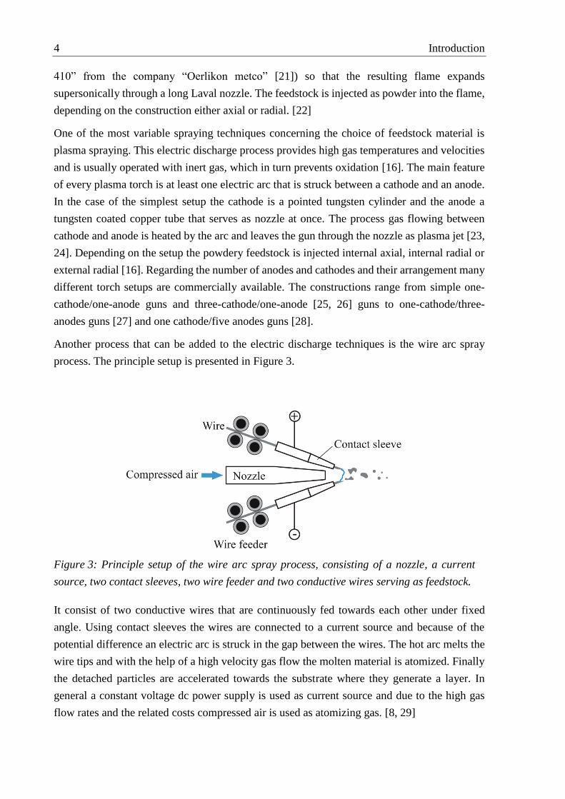
Another process that can be added to the electric discharge techniques is the wire arc spray
process. The principle setup is presented in Figure 3.
It consist of two conductive wires that are continuously fed towards each other under fixed
angle. Using contact sleeves the wires are connected to a current source and because of the
potential difference an electric arc is struck in the gap between the wires. The hot arc melts the
wire tips and with the help of a high velocity gas flow the molten material is atomized. Finally
the detached particles are accelerated towards the substrate where they generate a layer. In
general a constant voltage dc power supply is used as current source and due to the high gas
flow rates and the related costs compressed air is used as atomizing gas. [8, 29]
Figure 3: Principle setup of the wire arc spray process, consisting of a nozzle, a current
source, two contact sleeves, two wire feeder and two conductive wires serving as feedstock.

Introduction 5
Since the wires function as electrodes and feedstock at the same time the melting of the
complete coating material is guaranteed and consequently high coating efficiencies can be
reached. This advantage leads unavoidably to a problem that is topic of many research works.
Due to the different arc attachment on cathode (constricted) and anode (diffuse) the melting of
the wires and therefore the particle generation differs [30, 30, 31]. This asymmetric melting
behavior results in different temperature, velocity and size distributions between particles
detached form the cathode and particles detached form the anode [32–35]. Another negative
effect concerning the particle generation is the periodic fluctuation and re-ignition of the arc
caused by the periodic removal of the molten material [35]. Liao et al. [36] showed for example
that because of the fluctuations there are bimodal particle distributions both for the cathode wire
and the anode wire. An interesting approach to solve this problem is the use of pulsed current
controlling the arc movement [37].
All these research studies about wire arc spraying show that the particle generation is influenced
by many process parameters and that the resulting particles can vary with respect to
temperature, velocity and size. For this reason the wire arc spray process is an ideal
measurement object for particle diagnostics and is used in this work to test the developed
tomographic two-color-pyrometry.
1.1.2 Formation of thermal sprayed coatings
Every formation of thermal sprayed coatings starts with the particles generated from the
feedstock. In the case of wire- or rod-shaped feedstock there are process related less unmolten
particles presents than in the case of powdery feedstock [8]. The atomized particles are
transported by a stream of gas, whose influences they are exposed to during their flight time. If
the thermal spray process is performed in atmosphere the particles are additionally influenced
by the surrounding air and the oxygen, respectively [38]. Since the temperature of the particles
is above the melting point oxidation takes place very fast using metallic feedstock. In order to
clarify the influence of the temperature on the oxidation, the Arrhenius law [39, 40] presented
in Equation 1.1 can be used.
aE
RTk Ae
1.1
Using this equation the rate k of a chemical reaction with the activation energy aE can be
calculated. Besides the activation energy the rate depends on the gas constant R , the
temperature T and the frequency factor A . Whereby A takes the number of collisions with
the correct geometry into account [39] and is in turn slightly temperature dependent [8]. To
illustrate the significant influence of the temperature on the oxidation of metal particles, the
factor exp aE RT for iron depending on the temperature is presented in Figure 4. Therefore
the activation energy of iron 246.8 kJ molaE validated by Wilson et al. [41] is used. As we

6 Introduction
can see by increasing the temperature from 1850 K to 2150 K, the oxidation rate increases
approximately by one order of magnitude
Oxidation always occurs at the surface of a material and propagates inside through diffusion of
metal and oxygen into the oxide layer [41, 42]. However Deshpande et al. [43] and Espie et al.
[44] determined that there are both: a thin oxide sheet on the surface of the particles and oxide
inclusions within the particles. Responsible for the oxide fractions within the particles is
convective movement of the liquid oxides and metals resulting in continuous mixing [8, 43–
45]. Regarding small particles this effect may lead to complete oxidation as can be seen in the
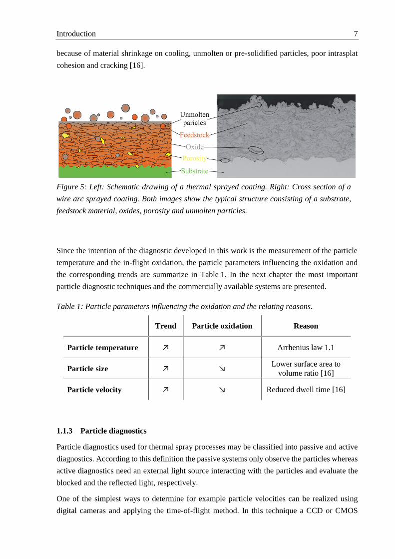
cross section presented in Figure 5.
The first molten particles that strike the substrate surface spread over and fill out the free spaces
of the surface. Consequently it is important to clean and to roughen the substrate surface in
order to achieve a good adhesion [8]. The cooling of the particles happens very fast because of
the great mass of the substrate compared to the particles and thus the impact of the following
particles takes place on a solid underground [46]. Through the continuously impact and
flattening of the particles a lamellar structure is formed. The principle setup of a thermal sprayed
coating is presented in Figure 5 on the left side. For comparison on the right side of Figure 5 a
cross section of a wire arc sprayed coating is illustrated. Besides the lamellar structure of the
feedstock, porosity, oxides and unmolten particles can be seen. The oxides are present in form
of so called oxide strings [16], solidified oxide droplets and oxide trapped inside the particles
[43]. As Li et al. [47] investigated for HVOF spraying of MCrAlY material there is, besides the
in-flight-oxidation, a second oxidation mechanism leading to oxide strings. This so called
post-impact oxidation is caused by the oxidation of the flattened particle surfaces taking place
until the next particles strike. The porosity within the coating occurs among other things
0.0E+00
1.0E-06
2.0E-06
3.0E-06
4.0E-06
5.0E-06
1850 1950 2050 2150 2250 2350 2450
exp(-
Ea
/RT
)
T [K]
Figure 4: Proportional factor exp(-Ea/RT) for the calculation of the iron oxidation rate
depending on the temperature T. For the calculation Ea=246.8 kJ/mol validated by Wilson et
al. [41] was used. R stands for the gas constant.
Introduction 7
because of material shrinkage on cooling, unmolten or pre-solidified particles, poor intrasplat
cohesion and cracking [16].
Since the intention of the diagnostic developed in this work is the measurement of the particle
temperature and the in-flight oxidation, the particle parameters influencing the oxidation and
the corresponding trends are summarize in Table 1. In the next chapter the most important
particle diagnostic techniques and the commercially available systems are presented.
Trend Particle oxidation Reason
Particle temperature ↗ ↗ Arrhenius law 1.1
Particle size ↗ ↘ Lower surface area to
volume ratio [16]
Particle velocity ↗ ↘ Reduced dwell time [16]
1.1.3 Particle diagnostics
Particle diagnostics used for thermal spray processes may be classified into passive and active
diagnostics. According to this definition the passive systems only observe the particles whereas
active diagnostics need an external light source interacting with the particles and evaluate the
blocked and the reflected light, respectively.
One of the simplest ways to determine for example particle velocities can be realized using
digital cameras and applying the time-of-flight method. In this technique a CCD or CMOS
Figure 5: Left: Schematic drawing of a thermal sprayed coating. Right: Cross section of a
wire arc sprayed coating. Both images show the typical structure consisting of a substrate,
feedstock material, oxides, porosity and unmolten particles.
Table 1: Particle parameters influencing the oxidation and the relating reasons.
8 Introduction
camera acquires images of the spray plume, whereby the exposure time is chosen in a way that
the flying particles leave bright traces on the images. With the help of the trace length
determined using image processing methods, the image scale and the adjusted exposure time
the velocity of single particles can finally be calculated. It is obvious that this method can only
be applied to thermal spray processes that generate luminous particles. Matz et al. [48] for
example used the PVI-system from the company “Zierhut Messtechnik GmbH” to investigate
the influence of the nozzle setup on particle velocities in wire arc spraying.
Another particle diagnostic using a digital camera is the SprayWatch from the company “Oseir”
[49]. Compared to the PVI this system additionally enables the measurement of particle
temperatures applying the principle of two-color-pyrometry. To acquire particle images at two
different wavelength bands two small stripes of the CCD sensor are covered with different
filters. In order to combine velocity and temperature measurement the camera records an image
with short exposure time followed by an image with long exposure time. The short exposed
image (part without filter in front) shows the typical particle traces and can be evaluated by
means of the time-of-flight method. The long exposed image (double-stripe part) is used to
calculate particle temperatures by means of two-color-pyrometry. Additionally the SprayWatch
can be transformed to an active diagnostic by applying a high power pulsed laser diode module
called HiWatch. This option enables the measurement of non-luminous particles such as
cold-sprayed particles [50, 51].
Vattulainen et al. [52] present another possibility to measure particle velocities and
temperatures using a single camera. In their setup a custom double mirror is used to record the
flying particles at two different wavelength bands. The first surface of the mirror reflects
radiation in the visible band the second surface in the near-IR band. The resulting images show
two overlapping traces for each particle that can in turn be evaluated by means of the
time-of-flight method and two-color-pyrometry.
The PVI as well as the SprayWatch and the diagnostic developed by Vattulainen et al. [52] are
easy to handle and to adjust but because of the projection of the spray plume on single two
dimensional sensors the information in direction of observation gets lost. As a consequence one
velocity component of the particle trajectories is missing and no statements can be made about
the three dimensional expansion of the spray plume.
In [53] a new measurement technique is suggested in order to remedy this lack of information
by using several cameras positioned around the spray plume simultaneously acquiring images
with short exposure times. With the help of image processing methods and a so called sinus-fit
the position and the three dimensional trajectories of single particles can be calculated. The
principle setup for the so called tomographic particle localization and velocity measurement is
presented on the left side of Figure 6. An example for a measured particle trajectory distribution
is shown on the right side.

Introduction 9
Another passive particle diagnostic is the DPV-system from the company “Tecnar”. The
function of this diagnostic is well described in [54–57] and can be explained based on Figure 7.
The particles flying through the measurement volume of the DPV are projected onto the
entrance of a fiber, which in turn is covered with a two-slit photomask. The optical signal is
parallelized and divided with the help of a lens and a dichroitic mirror. Using two interference
filters with different central wavelengths and two lenses the signal is projected onto
photodetector 1 and photodetector 2.
On the right side of Figure 7 the signals received by the two photodetectors are illustrated. As
can be seen the signals generated by one particle show two peaks, which in turn can be used to
determine the time t needed to cover the distance s between the two slits. The particle
Figure 6: Principle setup for tomographic particle localization and velocity measurement
(left) and an example for a particle trajectory distribution (right) measured with this
diagnostic. Both adopted from [53].
Figure 7: Schematic drawing of the DPV setup and the voltage signals received from the
photodetectors. According to [54, 55].
10 Introduction
velocity is finally given by P iv M s t , where
iM stands for the image scale of the sensor
head. For the determination of the particle temperatures again the principle of
two-color-pyrometry is used, whereby the assumption is made that the particles behave like
gray bodies meaning that their emissivities are independent on the wavelength. With the help
of the temperature and the energy detected in one channel the particle diameter can be calculated
assuming spherical particles and doing an energy correction for particles that are not fully seen
in both slits [57]. Because for this method the emissivity of the particles has to be known, a
complex calibration of the DPV has to be performed using a powder with known size
distribution [54, 55].
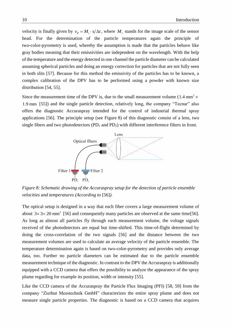
Since the measurement time of the DPV is, due to the small measurement volume ( 21.4 mm
1.9 mm [55]) and the single particle detection, relatively long, the company “Tecnar” also
offers the diagnostic Accuraspray intended for the control of industrial thermal spray
applications [56]. The principle setup (see Figure 8) of this diagnostic consist of a lens, two
single fibers and two photodetectors (PD1 and PD2) with different interference filters in front.
The optical setup is designed in a way that each fiber covers a large measurement volume of
about 33 3 20 mm [56] and consequently many particles are observed at the same time[56].
As long as almost all particles fly through each measurement volume, the voltage signals
received of the photodetectors are equal but time-shifted. This time-of-flight determined by
doing the cross-correlation of the two signals [56] and the distance between the two
measurement volumes are used to calculate an average velocity of the particle ensemble. The
temperature determination again is based on two-color-pyrometry and provides only average
data, too. Further no particle diameters can be estimated due to the particle ensemble
measurement technique of the diagnostic. In contrast to the DPV the Accuraspray is additionally
equipped with a CCD camera that offers the possibility to analyze the appearance of the spray
plume regarding for example its position, width or intensity [55].
Like the CCD camera of the Accuraspray the Particle Flux Imaging (PFI) [58, 59] from the
company “Zierhut Messtechnik GmbH” characterizes the entire spray plume and does not
measure single particle properties. The diagnostic is based on a CCD camera that acquires
Figure 8: Schematic drawing of the Accuraspray setup for the detection of particle ensemble
velocities and temperatures (According to [56]).

Introduction 11
images with long exposure time (320 ms [58]) and approximates the smoothed emission of the
spray plume with ellipses. Because of the quickly available information of the whole spray
plume and the low technical effort (only one single camera, no calibration), this diagnostic is
perfectly qualified for online control of thermal spray processes. Hartz-Behrend et al. [4] for
example applied the PFI as sensor in order to control the wire arc spray process using artificial
neural networks. For research purposes the PFI is not suitable, since selected particle properties
have to be known in order to be able to identify the parameters influencing for example the
coating formation.
An example for an active particle diagnostic based on digital cameras is the Particle Image
Velocimetry (PIV). In this method two consecutive laser flashes illuminate the measurement
volume of the diagnostic and the camera acquires either two single images or one
double-exposed image synchronized with the laser. The images are evaluated using particle
tracking, auto-correlation or cross-correlation methods in order to calculate the spatial distance
between matching particle pairs. By means of known exposure time a two dimensional particle
trajectory field can finally be determined. [60]
The disadvantage of measuring only two velocity components can be solved by tomographic
3D-PIV [61]. Here three dimensional particle distributions are reconstructed by means of
tomography using several images simultaneously recorded form different directions. The three
dimensional trajectory distribution again is calculated with the help of 3D cross-correlation and
the known exposure time.
A more complex technique to measure particle velocities is the Laser Doppler Anemometry
(LDA). This laser based diagnostic adopted from experimental fluid mechanics is usually
applied for point wise velocity measurement of a flow using tracer particles [62, 63]. Since in
the case of thermal spraying “tracer particles” are process related present anyway and their
properties are of particular interest concerning coating formation, the transfer of LDA is
obvious. The principle setup of an LDA-system designed for thermal spray applications is
shown in Figure 9 on the left side. This setup already used for the measurement of particle
velocities during the plasma-spray process [64] was developed by Mayr [65] and Reusch [66],
and is also used in this work. On the right side of Figure 9 an enlargement of the measurement
volume including the wave, velocity and observation direction vectors is shown. The
measurement volume is generated by crossing two laser beams under the angle . In the
crossing zone an interference pattern develops that interacts with the flying through particles.
The scattered light is collected by a lens and projected onto a photo multiplier, which in turn
generates a voltage signal. Since the particle sizes in thermal spraying range from several µm
up to some 10 µm the scattering mechanisms occurring are Mie-scattering and normal optical
reflection, refraction and diffraction [66]. The simplest way to explain the LDA is the
interference fringe model that is strictly speaking only valid for particles smaller than the
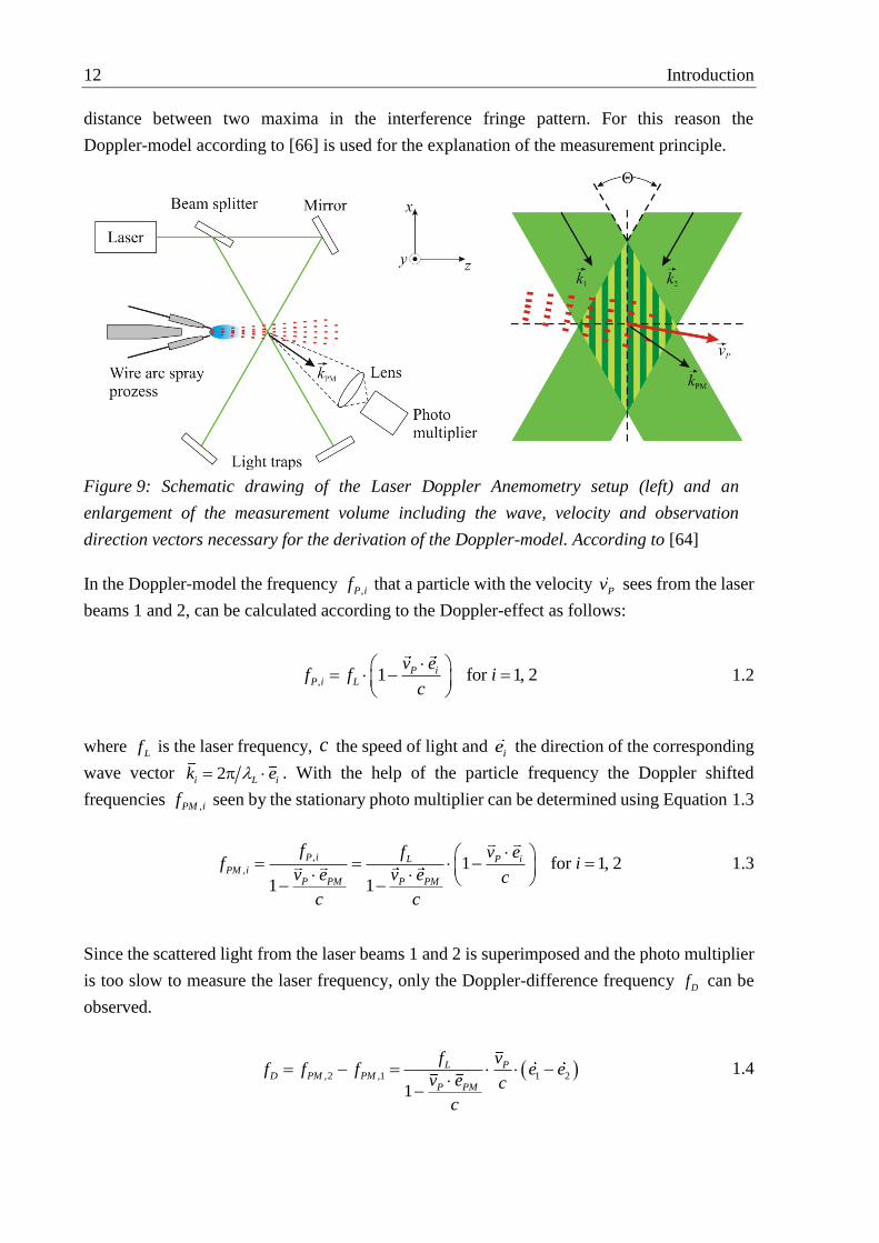
12 Introduction
distance between two maxima in the interference fringe pattern. For this reason the
Doppler-model according to [66] is used for the explanation of the measurement principle.
In the Doppler-model the frequency ,P if that a particle with the velocity Pv sees from the laser
beams 1 and 2, can be calculated according to the Doppler-effect as follows:
, 1 for 1, 2P iP i L
v ef f i
c
1.2
where Lf is the laser frequency, c the speed of light and
ie the direction of the corresponding
wave vector 2i L ik e . With the help of the particle frequency the Doppler shifted
frequencies ,PM if seen by the stationary photo multiplier can be determined using Equation 1.3
,
, 1 for 1, 2
1 1
P i L P iPM i
P PM P PM
f f v ef i
v e v e c
c c
1.3
Since the scattered light from the laser beams 1 and 2 is superimposed and the photo multiplier
is too slow to measure the laser frequency, only the Doppler-difference frequency Df can be
observed.
,2 ,1 1 2
1
L PD PM PM
P PM
f vf f f e e
v e c
c
1.4
Figure 9: Schematic drawing of the Laser Doppler Anemometry setup (left) and an
enlargement of the measurement volume including the wave, velocity and observation
direction vectors necessary for the derivation of the Doppler-model. According to [64]
Introduction 13
As velocities of thermal spray particles are much smaller than the speed of light ( 1Pv c ),
Equation 1.4 can be simplified as follows:
1 2L
D P
ff v e e
c 1.5
This equation is independent on the observation direction PMe . Using
L Lf c and calculating
1 2e e with the geometrical relations in Figure 9, Df is given by
,
12sin
2D P x
L
f v
1.6
Finally the velocity component in x -direction can be determined by solving Equation 1.6 for
,P xv and extracting Df out of the voltage signal measured with the photo multiplier. Besides
particle velocities also particle rates dn dt can be measured using LDA. The limitations of the
presented LDA-diagnostic are the determination of only the velocity component that is
perpendicular to the fringe pattern and the point wise measurement technique. The disadvantage
of missing velocity components can be solved through applying an additional pair of crossing
laser beams, whose interference pattern is turned 90° compared to the first one [62]. However,
the point wise measurement remains and consequently the time consuming scanning of a
measurement pattern is necessary in order to achieve three dimensional information of the spray
plume.
Another laser based method to measure particle velocities and rates is the Laser-Two-Focus
(L2F) diagnostic. L2F in principle works like a light barrier, whereby the scattered light of
particles flying through the measurement volumes of two focused laser beams is measured. By
using the distance between the two laser points and the measured time delay, the particle
velocity component perpendicular to the laser beams can be determined.
All above mentioned diagnostics, except the DPV, are not able to measure the particle size.
Even the DPV only derives the size from measured particle emissions, whereby a complex
calibration procedure is necessary and spherical particles are assumed. A diagnostic that enables
the direct determination of the particle size is the Phase Doppler Anemometry (PDA). The setup
of this diagnostic is similar to the LDA setup, with the sole difference that a second detector
(lens & photo multiplier) positioned under a different elevation angle additionally observes the
measurement volume. If the particles are spherical both detectors measure the same LDA-burst
time shifted. This time is equal to a phase difference, which in turn is proportional to the radius
of the particles. In summary the PDA enables the point wise measurement of single particle
velocities and sizes, whereby the particles have to be spherical. [67]
14 Introduction
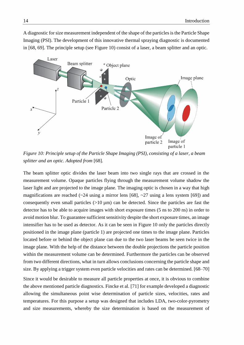
A diagnostic for size measurement independent of the shape of the particles is the Particle Shape
Imaging (PSI). The development of this innovative thermal spraying diagnostic is documented
in [68, 69]. The principle setup (see Figure 10) consist of a laser, a beam splitter and an optic.
The beam splitter optic divides the laser beam into two single rays that are crossed in the
measurement volume. Opaque particles flying through the measurement volume shadow the
laser light and are projected to the image plane. The imaging optic is chosen in a way that high
magnifications are reached (~24 using a mirror lens [68], ~27 using a lens system [69]) and
consequently even small particles (>10 µm) can be detected. Since the particles are fast the
detector has to be able to acquire images with short exposure times (5 ns to 200 ns) in order to
avoid motion blur. To guarantee sufficient sensitivity despite the short exposure times, an image
intensifier has to be used as detector. As it can be seen in Figure 10 only the particles directly
positioned in the image plane (particle 1) are projected one times to the image plane. Particles
located before or behind the object plane can due to the two laser beams be seen twice in the
image plane. With the help of the distance between the double projections the particle position
within the measurement volume can be determined. Furthermore the particles can be observed
from two different directions, what in turn allows conclusions concerning the particle shape and
size. By applying a trigger system even particle velocities and rates can be determined. [68–70]
Since it would be desirable to measure all particle properties at once, it is obvious to combine
the above mentioned particle diagnostics. Fincke et al. [71] for example developed a diagnostic
allowing the simultaneous point wise determination of particle sizes, velocities, rates and
temperatures. For this purpose a setup was designed that includes LDA, two-color-pyrometry
and size measurements, whereby the size determination is based on the measurement of
Figure 10: Principle setup of the Particle Shape Imaging (PSI), consisting of a laser, a beam
splitter and an optic. Adopted from [68].

Introduction 15
absolute scattered laser light. By using this combination of diagnostics important results
concerning the plasma particle interaction could be obtained.
After the comprehensive explanation of the particle diagnostics used in industry and in research
and development, in the next chapter the reasons are discussed, why further research on this
topic is still necessary. For a better overview the known diagnostics and their measured
quantities are summarized in Table 2.
Diagnostic v s T dn/dt Dimension Comment
PVI 2D
SprayWatch 2D
Vattulainen [52] 2D
Kirner [53] 3D
DPV 0D
Accuraspray 0D Particle ensemble
measurement
PFI 2D Qualitative evaluation of
the whole spray plume
PIV 2D Possibility of 3D
measurement
LDA 0D
L2F 0D
PDA 0D
PSI 0D
Fincke [71] 0D
Table 2: Summary of the known particle diagnostics and their measured quantities (v:
particle velocity, s: size, T: particle surface temperature, dn/dt: particle rate). The
geometrical dimension of the results are listed, too.

16 Introduction
1.2 Need of further research
Besides the adhesion and the porosity, the oxide content is one of most important factors
influencing the quality of metallic thermal sprayed coatings. Negative effects of oxides included
in coatings are for example decreased hardness or decreased cohesion between splats leading
to reduced toughness and cracking [72, 73]. However, there are not only disadvantages, oxides
may also increase the bonding to the substrate [72] or improve the resistance to compressive
loading [74]. Since in-flight oxidation of the particles mainly contributes to the oxide content
[43, 44, 72] the in-situ measurement of particle properties is indispensable for process control
and evaluation. As it can be seen on the basis of Table 1 the velocity as well as the size and the
temperature of the particles influence the in-flight oxidation. Consequently all three parameters
have to be known in order to draw reliable conclusions concerning the degree of oxidation. As
it can be seen in Table 2 there are only two diagnostics that are able to measure all necessary
particle parameters at once. On the one hand the DPV requiring a complex calibration and on
the other hand the experimental setup of Fincke et al. [71] designed for research. Of course also
other methods could be combined, but it is obvious that in any case a point by point
measurement is necessary to get the velocity, the size and the temperature. And in order to
achieve spatial resolved data of the whole spray plume the time consuming scanning of a
measurement pattern is unavoidable. Furthermore even determined particle velocities, sizes and
temperatures only allow qualitative or comparing statements regarding the oxidation, since it is
very difficult to estimate the chemical influence of the process gas and the surrounding
environment.
For these reasons, the aim of this work is the development of a diagnostic enabling the
quantitative determination of particle in-flight oxidation along the spraying direction. The idea
behind this innovative measurement technique is based on two-color-pyrometry. By observing
the spray plume at two different wavelength bands and assuming gray body behavior an average
surface temperature can be calculated. With the help of the known temperature and the
intensities measured at one of the two wavelength bands, finally the change in emissivity caused
by oxidation can be estimated. Further particle parameters that are needed as input for the model
are measured with established diagnostics.
The recording and evaluation of the raw data is done by means of tomography. Through the
combination of two-color-pyrometry and tomography three dimensional intensity and
temperature distributions can be determined. The application of tomography on a thermal spray
plume consisting of opaque particles is a completely new approach. In the past tomographic
measurement techniques in thermal spraying have only been used for the investigation of
plasma jets [75, 76].
Two-color-pyrometry 17
2 Two-color-pyrometry
The two-color-pyrometry is an optical method for the contactless measurement of surface
temperatures of solid bodies. In this measuring procedure the radiation of an object is observed
at two different narrow wavelength regions and it is assumed that the emissivities of the surface
at these two wavelengths are approximately similar. For the physical understanding of
two-color-pyrometry the theoretical bases of thermal radiation have to be known. In the
following chapter these are summarized and explained.
2.1 Theoretical bases of thermal radiation and two-color-pyrometry
The thermal radiation coming up against a body interacts in three different ways. It is partially
reflected by the surface (reflectivity ), partially absorbed by the body (absorptivity ) and
partially transmitted through the body (transmissivity ). Since the incident radiation has to be
the sum of the interacting radiation, the following relation can be written:
1 2.1
The thermal radiation of bodies has been described for the first time by Gustav Kirchhoff [77].
He showed that the radiation absorbed by a body in thermal equilibrium is emitted in the same
scale. This legality can be expressed by the absorptivity and the emissivity :
2.2
A special king of radiation is the so called black body radiation. A black body absorbs the whole
incident radiation, so that and are equal zero and it follows for and :
1 2.3
Josef Stefan [78] and Ludwig Boltzmann [79] discovered the dependence of the thermal
radiated power of a black body on the temperature. They postulated that the power P emitted
over the whole wavelength region by the surface A of a black body is the product precisely of
this surface, the Stefan-Boltzmann-constant and the fourth power of the absolute
temperature T of the black body.
4P AT 2.4
The first one describing the thermal radiation in dependence on the temperature and the
wavelength was Wilhelm Wien [80]. The Wien distribution law[81] exactly describes the
spectrum of the thermal radiation of a black body for short wavelengths, however for long
18 Two-color-pyrometry
wavelengths the law does not fit experimental data. The spectral exitance depending on the
temperature T and the wavelength can be calculated using Equation 2.5 [81].
1
52
1,
exps
CM T
C
T
2.5
Where 2
1 2C hc , 2 /C hc k , h is Planck’s constant, c is the speed of light and k is the
Boltzmann constant. The discrepancy in the Wien distribution law for long wavelengths could
be solved by Planck’s law. This law, postulated by Max Planck in the year 1900, describes the
spectral exitance sM of a black body depending on his temperature T at a single wavelength
[82–84]:
1
52
1,
exp 1s
CM T
C
T
2.6
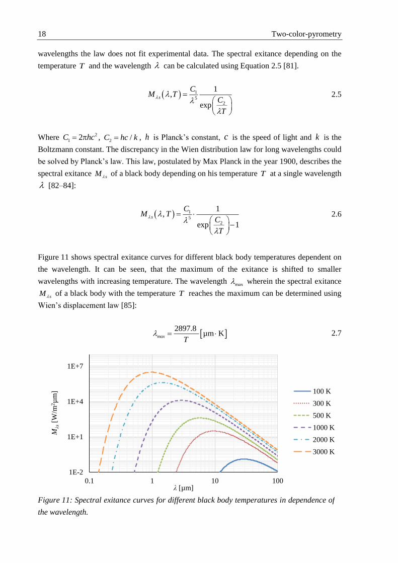
Figure 11 shows spectral exitance curves for different black body temperatures dependent on
the wavelength. It can be seen, that the maximum of the exitance is shifted to smaller
wavelengths with increasing temperature. The wavelength max wherein the spectral exitance
sM of a black body with the temperature T reaches the maximum can be determined using
Wien’s displacement law [85]:
2897.8
µm KmaxT
2.7
1E-2
1E+1
1E+4
1E+7
0.1 1 10 100
Mλs
[W/m
2µ
m]
λ [µm]
100 K
300 K
500 K
1000 K
2000 K
3000 K
Figure 11: Spectral exitance curves for different black body temperatures in dependence of
the wavelength.

Two-color-pyrometry 19
A black body is idealized and does in reality not exist in this form. The behavior of a black
body surface can e.g. be approximated by a narrow opening of a cavity in a metal cylinder [85].
For real bodies the absorptivity, the transmissivity, the reflectivity and the emissivity depend
on the direction, the wavelength, the temperature [86] and on surface properties like e.g.
roughness [87]. Figure 12 shows the principle behavior of the black, gray and real body
emissivity depending on the wavelength. As we can see, the emissivity of a black body is
constant and equals one, the emissivity of a gray body is also constant, but since the
transmissivity and the reflectivity are not equal zero, the emissivity is smaller than one. The
real body emissivity is also smaller than one and in general changes with the wavelength and
the temperature. Accordingly for a real body the spectral exitance has to be multiplied by the
emissivity to get the spectral radiant exitance ,M T :
, , ,sM T T M T 2.8
Since it is difficult and sometimes impossible to measure the emissivity, it is necessary to use
a measurement method for the determination of the surface temperature that works
independently on this parameter. The most important technique used in industry and research
is the two-color-pyrometry. In the following chapters the principle of two-color-pyrometry and
the technical realization in the context of this work are explained.
The basic principle of the two-color-pyrometry is the observation of the measurement object at
two different wavelengths 1 and
2 . For each wavelength the spectral radiant exitance has to
be calculated and divided by each other, resulting in the quotient Q :
1 1
2 2
, ,
, ,
s
s
T M TQ T
T M T
2.9
By the assumption that the observed object behaves like a gray body it follows
0
0.2
0.4
0.6
0.8
1
0.1 1 10 100 1000
ε(λ
)
λ [µm]
black body
gray body
real body
Figure 12: Principle emissivities of a black, a gray and a real body depending on the
wavelength.
20 Two-color-pyrometry
1 2, ,T T 2.10
and consequently the emissivities in Equation 2.9 can be canceled. The remaining
Equation 2.11 for the determination of the quotient Q just depends on the temperature T .
5 22
2
5 21
1
exp 1
exp 1
C
TQ T
C
T
2.11
Because Equation 2.11 cannot directly be solved for T , measured intensity quotients have to
be compared with quotients calculated with Equation 2.11.
2.2 Technical realization
In the following chapters the technical realization of the two-color-pyrometry is discussed.
Particularly the setup, the selection of the components, the optical properties, the temperature
calculation method and the calibration of the system are presented in detail.
2.2.1 Experimental setup
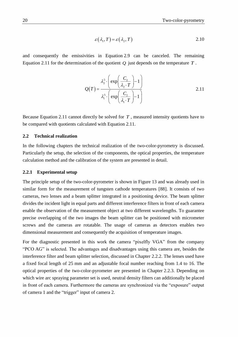
The principle setup of the two-color-pyrometer is shown in Figure 13 and was already used in
similar form for the measurement of tungsten cathode temperatures [88]. It consists of two
cameras, two lenses and a beam splitter integrated in a positioning device. The beam splitter
divides the incident light in equal parts and different interference filters in front of each camera
enable the observation of the measurement object at two different wavelengths. To guarantee
precise overlapping of the two images the beam splitter can be positioned with micrometer
screws and the cameras are rotatable. The usage of cameras as detectors enables two
dimensional measurement and consequently the acquisition of temperature images.
For the diagnostic presented in this work the camera “pixelfly VGA” from the company
“PCO AG” is selected. The advantages and disadvantages using this camera are, besides the
interference filter and beam splitter selection, discussed in Chapter 2.2.2. The lenses used have
a fixed focal length of 25 mm and an adjustable focal number reaching from 1.4 to 16. The
optical properties of the two-color-pyrometer are presented in Chapter 2.2.3. Depending on
which wire arc spraying parameter set is used, neutral density filters can additionally be placed
in front of each camera. Furthermore the cameras are synchronized via the “exposure” output
of camera 1 and the “trigger” input of camera 2.
Two-color-pyrometry 21
2.2.2 Camera, interference filter and beam splitter selection
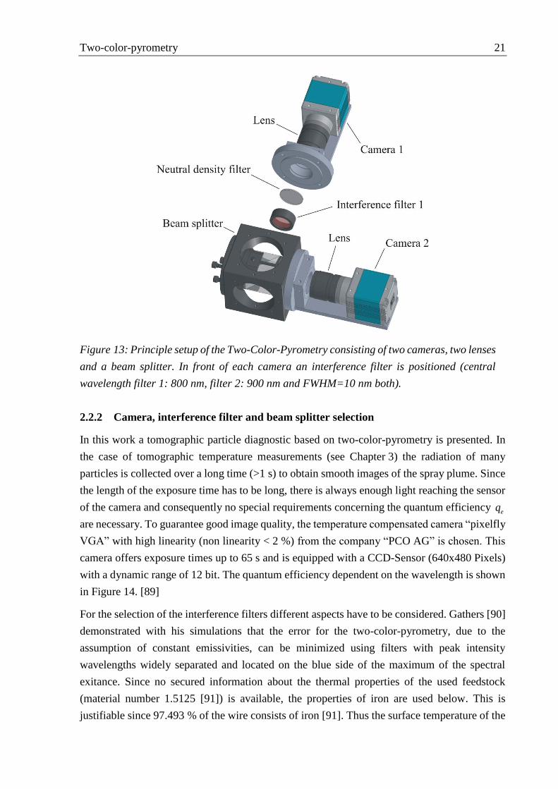
In this work a tomographic particle diagnostic based on two-color-pyrometry is presented. In
the case of tomographic temperature measurements (see Chapter 3) the radiation of many
particles is collected over a long time (>1 s) to obtain smooth images of the spray plume. Since
the length of the exposure time has to be long, there is always enough light reaching the sensor
of the camera and consequently no special requirements concerning the quantum efficiency eq
are necessary. To guarantee good image quality, the temperature compensated camera “pixelfly
VGA” with high linearity (non linearity < 2 %) from the company “PCO AG” is chosen. This
camera offers exposure times up to 65 s and is equipped with a CCD-Sensor (640x480 Pixels)
with a dynamic range of 12 bit. The quantum efficiency dependent on the wavelength is shown
in Figure 14. [89]
For the selection of the interference filters different aspects have to be considered. Gathers [90]
demonstrated with his simulations that the error for the two-color-pyrometry, due to the
assumption of constant emissivities, can be minimized using filters with peak intensity
wavelengths widely separated and located on the blue side of the maximum of the spectral
exitance. Since no secured information about the thermal properties of the used feedstock
(material number 1.5125 [91]) is available, the properties of iron are used below. This is
justifiable since 97.493 % of the wire consists of iron [91]. Thus the surface temperature of the
Figure 13: Principle setup of the Two-Color-Pyrometry consisting of two cameras, two lenses
and a beam splitter. In front of each camera an interference filter is positioned (central
wavelength filter 1: 800 nm, filter 2: 900 nm and FWHM=10 nm both).
22 Two-color-pyrometry
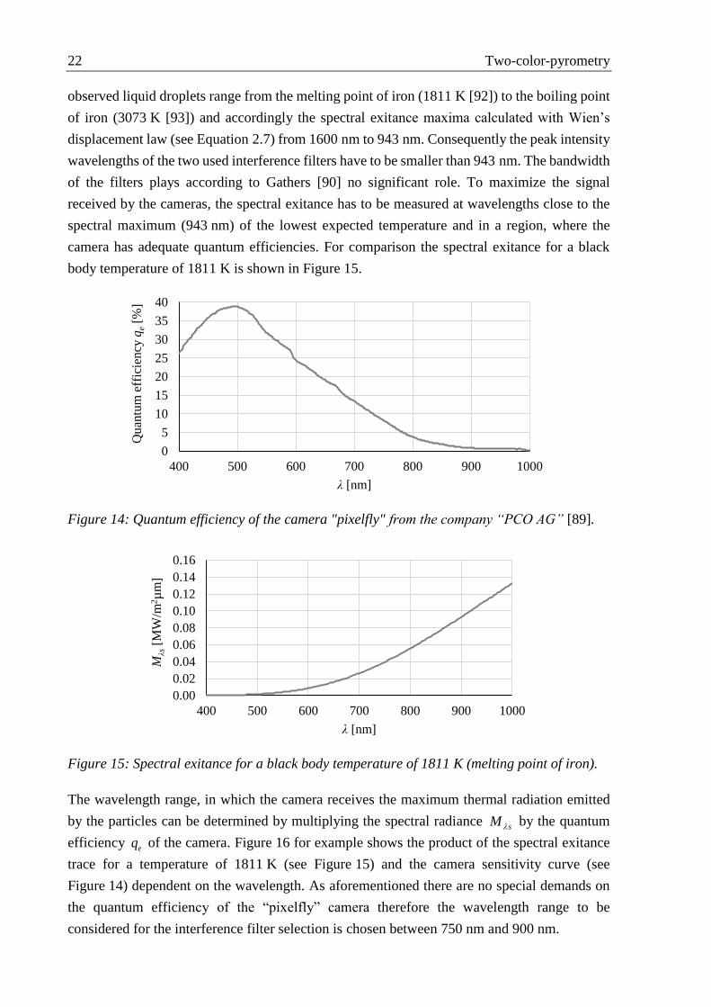
observed liquid droplets range from the melting point of iron (1811 K [92]) to the boiling point
of iron (3073 K [93]) and accordingly the spectral exitance maxima calculated with Wien’s
displacement law (see Equation 2.7) from 1600 nm to 943 nm. Consequently the peak intensity
wavelengths of the two used interference filters have to be smaller than 943 nm. The bandwidth
of the filters plays according to Gathers [90] no significant role. To maximize the signal
received by the cameras, the spectral exitance has to be measured at wavelengths close to the
spectral maximum (943 nm) of the lowest expected temperature and in a region, where the
camera has adequate quantum efficiencies. For comparison the spectral exitance for a black
body temperature of 1811 K is shown in Figure 15.
The wavelength range, in which the camera receives the maximum thermal radiation emitted
by the particles can be determined by multiplying the spectral radiance sM by the quantum
efficiency eq of the camera. Figure 16 for example shows the product of the spectral exitance
trace for a temperature of 1811 K (see Figure 15) and the camera sensitivity curve (see
Figure 14) dependent on the wavelength. As aforementioned there are no special demands on
the quantum efficiency of the “pixelfly” camera therefore the wavelength range to be
considered for the interference filter selection is chosen between 750 nm and 900 nm.
0
5
10
15
20
25
30
35
40
400 500 600 700 800 900 1000
Qu
antu
m e
ffic
ien
cy q
e[%
]
λ [nm]
0.00
0.02
0.04
0.06
0.08
0.10
0.12
0.14
0.16
400 500 600 700 800 900 1000
Mλs
[MW
/m2µ
m]
λ [nm]
Figure 14: Quantum efficiency of the camera "pixelfly" from the company “PCO AG” [89].
Figure 15: Spectral exitance for a black body temperature of 1811 K (melting point of iron).
Two-color-pyrometry 23
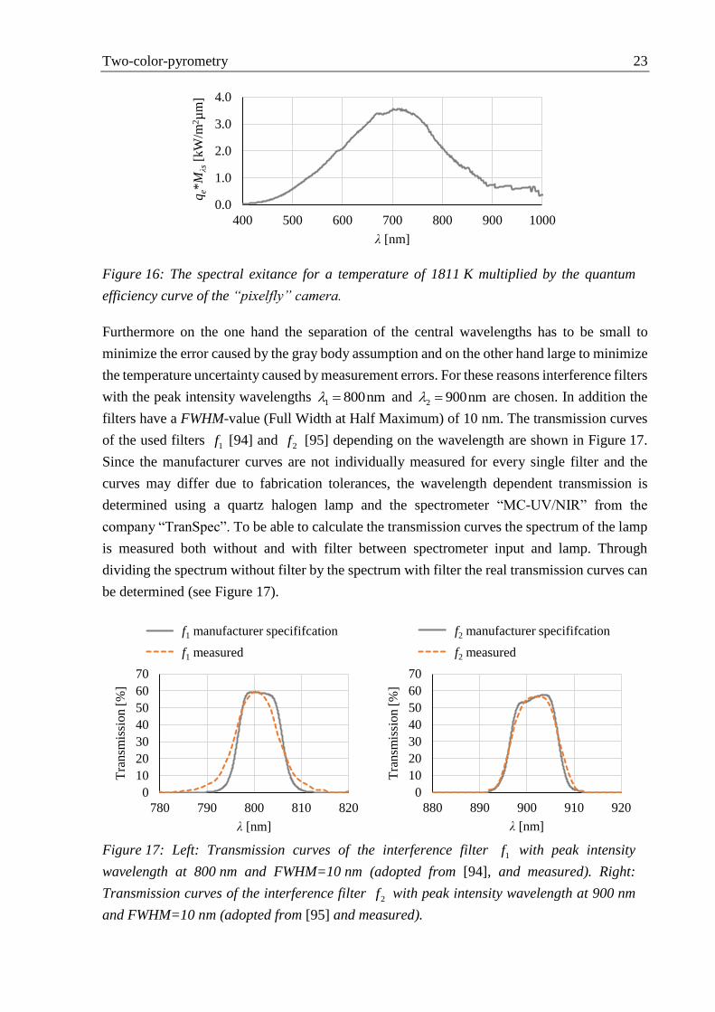
Furthermore on the one hand the separation of the central wavelengths has to be small to
minimize the error caused by the gray body assumption and on the other hand large to minimize
the temperature uncertainty caused by measurement errors. For these reasons interference filters
with the peak intensity wavelengths 1 800nm and
2 900nm are chosen. In addition the
filters have a FWHM-value (Full Width at Half Maximum) of 10 nm. The transmission curves
of the used filters 1f [94] and
2f [95] depending on the wavelength are shown in Figure 17.
Since the manufacturer curves are not individually measured for every single filter and the
curves may differ due to fabrication tolerances, the wavelength dependent transmission is
determined using a quartz halogen lamp and the spectrometer “MC-UV/NIR” from the
company “TranSpec”. To be able to calculate the transmission curves the spectrum of the lamp
is measured both without and with filter between spectrometer input and lamp. Through
dividing the spectrum without filter by the spectrum with filter the real transmission curves can
be determined (see Figure 17).
0.0
1.0
2.0
3.0
4.0
400 500 600 700 800 900 1000
qe*
Mλs
[kW
/m2µ
m]
λ [nm]
0
10
20
30
40
50
60
70
780 790 800 810 820
Tra
nsm
issi
on
[%
]
λ [nm]
f₁ manufacturer specification
f₁ measured
f1 manufacturer specififcation
f1 measured
0
10
20
30
40
50
60
70
880 890 900 910 920
Tra
nsm
issi
on
[%
]
λ [nm]
f2 manufacturer specification
f₁ measured
f2 manufacturer specififcation
f2 measured
Figure 16: The spectral exitance for a temperature of 1811 K multiplied by the quantum
efficiency curve of the “pixelfly” camera.
Figure 17: Left: Transmission curves of the interference filter 1f with peak intensity
wavelength at 800 nm and FWHM=10 nm (adopted from [94], and measured). Right:
Transmission curves of the interference filter 2f with peak intensity wavelength at 900 nm
and FWHM=10 nm (adopted from [95] and measured).
24 Two-color-pyrometry
The measurement error GBE caused by the gray body assumption is defined by the ratio of the
temperature error (real measuredT T ) and the measured temperature [96]. For the following
considerations the Wien approximation (see Equation 2.7) has to be solved for T resulting in
Equation 2.12 and for the determination of measuredT the ration
2 1/ has to be set one.
Furthermore it is assumed that the transmission curves of the interference filters are Dirac
functions.
2
2 1
5,1 2 1
5
,2 1 2
1 1
ln s
s
C
TM
M
2.12
The resulting Equation 2.13 [96, 97] (see derivation in the Appendix A.1) for GBE only depends
on the emissivities, the real temperature realT and the two central wavelengths
1 and 2 of the
interference filters.
1
2
2
1 2
,ln
,
1 1
real
real
realreal measuredGB
measured
TT
TT TE
TC
2.13
Taking the emissivities of liquid iron at 800 nm 800 nm, 1811K 0.3788 and at 900 nm
900 nm, 1811K 0.3687 calculated according to Watanabe et al. [98], the error due to gray
body assumption is 2.42 %GBE .
For the calculation of the temperature uncertainty caused by measurement errors the spectral
exitances in Equation 2.12 are approximated by the corresponding measured intensities I and
the ratio of the emissivities is set one:
2
2 1
5
1 1
5
2 2
1 1
ln
C
TI
I
2.14
The temperature error T can be estimated through the first order terms of a Taylor series as
long as the variations 1I and
2I of the measured intensities are small [99, 100]:
1 2
1 2
T TT I I
I I
2.15
Two-color-pyrometry 25
Equation 2.16 [96] (see Appendix A.1) presents the solution of Equation 2.15. It describes the
relative temperature error /T T dependent on the temperature T , the measured intensities,
their variations and the central wavelengths 1 and
2 .
1 2 1 2
2 2 1 1 2
T T I I
T C I I
2.16
As Equation 2.16 shows the measurement uncertainties (1 1/I I and
2 2/I I ) are amplified by
a factor that only depends on the temperature and the wavelengths of the used interference
filters. Choosing a wide separation of the central wavelengths decreases this factor and
consequently the relative temperature error, too. For the used interference filters (800 nm and
900 nm) and the expected temperatures (1811 K to 3073 K) the factor is between 0.9062 and
1.5378. Assuming a worst case measurement uncertainty of 50 countsI per pixel and an
80 % utilization of the dynamic range (“pixelfly” 12 bit) the temperature error ranges from
2.77 % to 4.69 %.
The last optical element that has to be chosen carefully is the beam splitter. Therefore a cube
optimized for the NIR region from the company “QIOPTIQ” with an edge length of 30 mm is
chosen. The beam splitter has a broadband antireflective-coating “ARB 2 NIR”, that guarantees
residual reflections smaller than 0.5 % in a wavelength region between 750 nm and 1050 nm
[101]. This special kind of coating is necessary to avoid multiple reflections between the sensor
surface and the beam splitter surface (see Figure 13).
2.2.3 Optical properties
The sector of the spray plume that can be analyzed using the two-color-pyrometer depends on
the measurement volume of the diagnostic. Particles in this volume appear in focus on the
acquired images and can be correctly evaluated. As Figure 18 shows, the dimension of the
measurement volume depends on the depth of field (DOF), the width W and the height H of the
object plane (green).
A point light source positioned in the object plane of a lens is exactly imaged to the image plane
or to be more precise to the sensor of the camera. If the source is moved out of focus it appears
as round spot, the so called circle of confusion (CoC). As long as the size of the CoC is smaller
than a pixel the image appears as if the object would be located in the object plane.
Consequently for the calculation of the DOF the diameter of the CoC has to be smaller than the
edge length of a pixel [102, 103].
The dimension of the DOF is restricted by the near limit ND and the far limit
FD relating to
the position of the lens. According to [103–106] ND ,
FD and DOF can be calculated using
Equation 2.17, 2.18 and 2.19. The limits depend on the object distance oS , the focal distance
f , the f-Number N and the diameter cd of the circle of confusion.

26 Two-color-pyrometry
2
2 ( )
oN
c o
S fD
f Nd S f
2.17
2
2 ( )
oF
c o
S fD
f Nd S f
2.18
F NDOF D D 2.19
The diagram in Figure 19 presents the DOF dependent on the object distance for the “pixelfly”
camera. The DOF in the diagram is calculated for the focal length 25 mmf , the f-Number
16N and the circle of confusion diameter 9.9 µmcd (edge length of a pixel [89]). As can
clearly be seen, the DOF increases with increasing object distance.
0
100
200
300
400
500
600
0 200 400 600 800 1000
DO
F[m
m]
So [mm]
Figure 18: Measurement volume of the two-color-pyrometer dependent on the depth of view
(DOF) and the object plane dimensions (green).
Figure 19: Depth of field (DOF) dependent on the object distance oS for the “pixelfly”.

Two-color-pyrometry 27
The calculated DOF for the object distance of the experimental setup (see Chapter 3.3.1) is
listed in Table 3. The width W and the height H of the object plane are dependent on the
resolution w h , the pixel edge length cd , the object distance
0S and the focal length f . The
dimensions can be calculated using Equation 2.20 and 2.21. In addition they are listed in
Table 3, too.
oc
S fW w d
f
2.20
oc
S fH h d
f
2.21
As it can be seen in Figure 18 the width and the height of the measurement volume changes
outside the object plane. In order to estimate if this distortion can be neglected the following
calculations are necessary. Figure 20 shows the geometrical relations for an object G
positioned directly in the object plane oS (green) and in the near limit
ND of the DOF (red).
If the object is positioned in the object plane it is projected to the image plane iS and the size
B of the image can be determined using Equation 2.22.
0
iSB G
S 2.22
The same object located in the near limit of the DOF namely is perceived to be in focus but is
stretched in the image plane iS compared to the image B . In order to be able to calculate the
Figure 20: Optical imaging of an object G exactly located in the object plane 0S and of the
same object located in the near DOF limit ND , whereat the image distance
iS (sensor
position) is constant. NB presents the blurred image and B the image in focus.

28 Two-color-pyrometry
extension NB of the blurred image, the distance
NX (see Figure 20) has to be determined with
the following equation:
N i
N
GX S
D 2.23
With the help of NX and B it follows for
NB :
2
NN
B XB
2.24
Finally the relation of NB to B can be determined using Equation 2.25.
1
12
N o
N
B S
B D
2.25
To get the relation of FB to B only
ND in Equation 2.25 has to be replaced by FD . All results
concerning the measurement volume of the experimental setup presented in this chapter are
listed in Table 3.
Pixel edge length [µm] 9.9
Resolution w × h 640 480
Object distance .. [mm] 625
Object plane width W [mm] 152.06
Object plane height H [mm] 114.05
Near limit of the depth of field ND [mm] 542.50
Far limit of the depth of field FD [mm] 737.08
Depth of field DOF [mm] 194.58
NB B 1.08
FB B 0.92
The values in the last two rows show that objects located in the near and far limit of the depth
of field are enlarged for 8 % and minimized for 8 %, respectively. This geometrical error may
Table 3: Important optical properties of the experimental setup dependent on the pixel edge
length of the “pixelfly” camera, the resolution of the camera and the object distance 0S .

Two-color-pyrometry 29
be negligible since the expansion of the measurement object (spray plume) is significantly
smaller than the DOF (see Chapter 3.3.2).
2.2.4 Temperature calculation
The real intensities 1I and
2I detected by the cameras with the two different interference filters
in front can be calculated using Equation 2.26 and 2.27.
1 1 1 / 1, , with 2e
s
e s s eI T K q f T M T d FWHM
2.26
2 2 2 / 2, , with 2e
s
e s s eI T K q f T M T d FWHM
2.27
Therefore the camera quantum efficiency eq and the transmission curves of the filters
1f and
2f have, besides the spectral radiant exitance, to be taken into account. Since the transmission
curves of the filters are not a Dirac function, the integral with respect to on the interval s
to e has to be formed. Furthermore calibration factors
1K and 2K , that include different
uncertainties, are necessary. One of the main problems responsible for the need of calibration
factors is the use of manufacturer data concerning the transmission curves of the filters (see
Figure 17) and the quantum efficiency of the camera (see Figure 14). As the exchange of the
components with nominally the same characteristic has shown, there is a large deviation and
the manufacturer data may only be used for reference. Further problems that have to be taken
into account are possible shifts of the central wavelengths caused by a tilt of the interference
filters [107] and the wavelength dependent reflection and transmission curves (50 % ± 3 %
[108]) of the beam splitter. Since the results of the integrals of Equation 2.26 and 2.27 indicate
the emitted power per square meter and the measured intensities are dimensionless quantities,
the calibration factors 1K and
2K must have the unit 2m W .
As already mentioned in Chapter 2.1 the assumption is made that the observed objects behave
like grey bodies and consequently the emissivities equal one and only depend on the
temperature:
, T T 2.28
By forming the quotient of 1I and
2I the emissivities can be canceled so that the resulting
Equation 2.29 only depends on the temperature, whereas the quotient of the calibration factors
can be written as 1 2/K K K .

30 Two-color-pyrometry
1
1
2
2
,
,
e
s
e
s
e s
e s
q f M T dI T
Q T KI T
q f M T d
2.29
Because from 1f ,
2f and eq only single values and no functions are available, the integrals in
Equation 2.29 cannot be solved and have to be approximated with the so called Riemann sum
[109]. The quotient Q dependent on T can finally be calculated using Equation 2.30.
2 /
1 1 1 1
2 /
2 /
2 2 2 2
2 /
,
,
FWHM
e s
i FWHM
FWHM
e s
i FWHM
q i f i M i T
Q T K
q i f i M i T
2.30
The constant step size has to be chosen small in order to minimize the error. The evaluation
of the data has shown that a step size of 0.5nm is sufficient for a good approximation of
the integrals. Figure 21 shows the quotient Q dependent of the temperature T calculated for
the transmission curves 1f and
2f , the quantum efficiency eq of the “pixelfly” camera and a
calibration factor of 0.1828K .
In order to determine a 2D-temperature distribution, the intensities measured by camera 1 have
to be divided by the ones measured by camera 2 (mQ ). As Equation 2.30 cannot be solved for
the temperature, the measured quotients mQ on position x and y of the quotient image have
to be compared with the calculated quotient Q T in order to determine the measured
temperature ,mT x y . If Q T is equal ,mQ x y it follows ,mT x y T .
0.0
0.2
0.4
0.6
0.8
1.0
1.2
1000 1500 2000 2500 3000 3500 4000
Q
T [K]
Figure 21: Quotient Q dependent on the temperature T calculated for the transmission
curves 1f and
2f , the quantum efficiency qe of the “pixelfly” camera, a calibration factor
of K = 0.1828 and a step size of Δλ=0.5 nm .

Two-color-pyrometry 31
2.2.5 Calibration of the two-color-pyrometer
For the estimation of the calibration factor K the miniature quartz halogen lamp “L7390A”
(tungsten filament) and a precision current source with four different levels are used. To be able
to calibrate the two-color-pyrometer the temperatures of the lamp for the four current values
have to be known. Therefore the spectra of the four levels (Figure 22) are measured using the
spectrometer “Aryelle” from the company “LBS-Berlin”.
The dimensionless recorded spectral intensity I of the lamp can be described by the
following equation:
0, , ,sI T k T M T 2.31
In this connection 0k [m³W-1] is a proportional factor that takes the geometrical dependence of
the radiation into account and , T is the emissivity of the lamp (tungsten filament). As the
results of Dmitriev et al. [110] and Larrabee et al. [111] in Figure 23 show, the emissivity of
tungsten for the estimated temperatures (2000 K – 3000 K) and the observed wavelength region
(500 nm – 800 nm) is almost constant. Thus , T and 0k can be summarized to the
proportional factor TH [m³W-1]. From Equation 2.6 and 2.31 it finally follows for ,I T :
0
20000
40000
60000
80000
100000
120000
140000
500 550 600 650 700 750 800
I (λ
, T
)
λ [nm]
Level 1
Level 2
Level 3
Level 4
Figure 22: Spectra of the miniature halogen lamp at four different current levels measured
with the spectrometer “Aryelle”

32 Two-color-pyrometry
1
52
1,
exp 1T
CI T H
C
T
2.32
The unknown parameter TH and T in this equation are determined by fitting Equation 2.32 to
the N measured discrete values ,i iI T by means of the least-square method. Therefore the
sum of square residuals R is calculated:
21
1 2
51
1, exp 1
2
N
i i T
i i i
C CR I T H
T
2.33
Since Equation 2.33 is a non-linear least-square problem, the Levenberg-Marquardt (LM)
algorithm is used for the calculation of the parameter vector ,TH Tp [112]. For this
iterative technique the Jacobian Matrix J of ,I T has to be determined (see Equation 2.34):
1 1, ,
, ,
, ,
T
i i
T
N N
T
I T I T
H T
I T I T
H T
I T I T
H T
IJ
p 2.34
with
1
5
2
, 1
exp 1
i
T i
i
I T C
H C
T
2.35
0.00
0.20
0.40
0.60
0.80
500 550 600 650 700 750 800
ε(λ
,2400 K
)
λ [nm]
Dmitriev
Larrabee
Figure 23: Emissivity of tungsten for 2400 K dependent on the wavelength measured by
Dmitriev et al. [110] and Larrabee et al. [111].

Two-color-pyrometry 33
and
2
1 2 2 2
6 2
,exp exp 1
i
T
i i i
I T C C C CH
T T T T
2.36
At the beginning of the LM method the starting point 0 0,TH T0p has to be chosen.
Subsequently in every iteration step the correction vector ,TH T pδ , that minimizes the
sum R of square residuals, has to be found. To get pδ the following system of linear equations
has to be solved:
T T pJ J E δ J ε 2.37
with µ as damping term, E as identity matrix and 1 1 , ... , , ... ,i i N NI I I I I I
as error vector. In Equation 2.37 TJ J can be combined to N and TJ to F and it follows:
pN E δ F 2.38
so that
212 1
11 1 12 1
12 21 1122
11
and T
NF F
N F N TT H
N N NN
N
. 2.39
The algorithm has to be repeated until the chosen abort criterion is fulfilled. The used starting
points and parameters are presented in the following listing of the complete algorithm:
1. Choosing starting point 0p (for all calculations
0
3 -11 m WTH and 0 10000 KT was
chosen)
2. Calculation of Rold, N and F using oldp and Equation 2.33 - Equation 2.37
3. Choosing damping term (for all calculation 1 was chosen)
4. Calculation of pδ using N, F, oldp and Equation 2.39
5. Calculation of new old pp p δ and newR using
newp
6. If new oldR R then double ,
old newR R and go to step 4
If new oldR R then
newoldp = p , old newR R and go to step 3
7. The iterations from step 3 to step 6 are done until new oldR R (local minimum of the
sum of square residuals R is reached)
34 Two-color-pyrometry
The diagram in Figure 24 shows the evolution of TnewH and
newT for the spectrum of level 1
dependent on the iteration step. The trends of the graphs indicate the convergence of the
algorithm and show that there is no significant change after 8 iterations.
In Table 4 the calculated temperatures refT and proportional factors TH for the four levels are
listed. At level 1 the algorithm was canceled after 11 iterations, at level 2 after 14 iteration, at
level 3 after 20 iterations and at level 4 after 19 iterations.
Level Current [A] KrefT 3 1[m W ]TH
1 4.82 2190 6.39·10-8
2 5.42 2351 6.82·10-8
3 6.11 2530 7.34·10-8
4 6.92 2723 8.12·10-8
The example in Figure 25 shows the measured spectrum (blue) of the halogen lamp at current
level 1 and the corresponding calculated spectrum (red). It can be seen that Equation 2.32 using
the calculated parameters of Table 4 is a good approximation for the measured values.
0
2000
4000
6000
8000
10000
0.00E+00
1.00E-08
2.00E-08
3.00E-08
4.00E-08
5.00E-08
6.00E-08
7.00E-08
8.00E-08
9.00E-08
0 2 4 6 8
T[K
]
HT
[m3W
-1]
Iteration No.
HTnew Tnew
Figure 24: Convergence of the parameters TnewH and
newT for the fit to the lamp spectrum
measured at current level 1 after nine iterations.
Table 4: Calculated temperatures refT and proportional factorsTH for the four different
current levels of the halogen lamp.

Two-color-pyrometry 35
As the two-color-pyrometer enables two dimensional measurements and consequently the
complete camera sensors are used, the calibration has to be done for every pixel. Responsible
therefore is the dependence of the transmittance and the reflectance of the beam splitter cube
on the incidence angle of light [113] and the reduction of the image brightness from the
periphery towards the center due to natural and optical vignetting [114, 115]. For this reason an
experimental setup, as shown in Figure 26, was arranged that consists of a holder for the
two-color-pyrometer and a device to move the calibration lamp. The vertical movement is done
by a hand driven linear axle and the horizontal movement by a stepper driven linear axle.
0
5000
10000
15000
20000
25000
500 550 600 650 700 750 800
I(λ
, T
)
λ [nm]
Level 1 Fit Level 1
Figure 25: Measured spectrum (blue) ,i iI T of the miniature halogen lamp at current
level 1 and the corresponding calculated spectrum (red) ,iI T
Figure 26: Experimental setup for the calibration of the two-color-pyrometer, consisting of
the calibration lamp that can be moved horizontal and vertical using a stepper motor driven
axle and a hand driven linear axle.
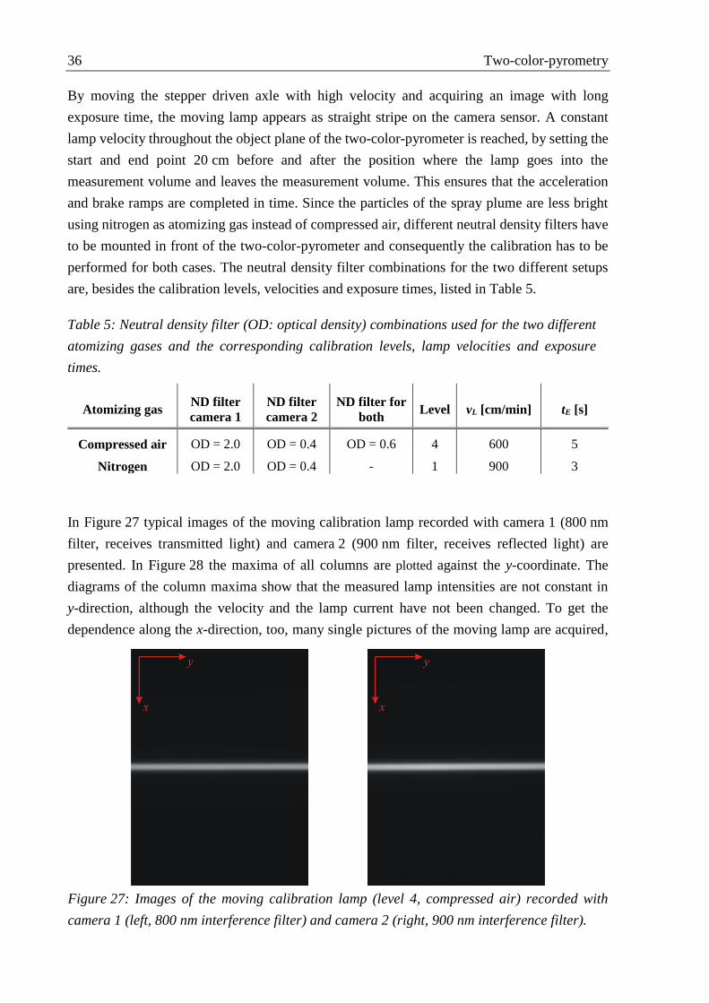
36 Two-color-pyrometry
By moving the stepper driven axle with high velocity and acquiring an image with long
exposure time, the moving lamp appears as straight stripe on the camera sensor. A constant
lamp velocity throughout the object plane of the two-color-pyrometer is reached, by setting the
start and end point 20 cm before and after the position where the lamp goes into the
measurement volume and leaves the measurement volume. This ensures that the acceleration
and brake ramps are completed in time. Since the particles of the spray plume are less bright
using nitrogen as atomizing gas instead of compressed air, different neutral density filters have
to be mounted in front of the two-color-pyrometer and consequently the calibration has to be
performed for both cases. The neutral density filter combinations for the two different setups
are, besides the calibration levels, velocities and exposure times, listed in Table 5.
Atomizing gas ND filter
camera 1
ND filter
camera 2
ND filter for
both Level vL [cm/min] tE [s]
Compressed air OD = 2.0 OD = 0.4 OD = 0.6 4 600 5
Nitrogen OD = 2.0 OD = 0.4 - 1 900 3
In Figure 27 typical images of the moving calibration lamp recorded with camera 1 (800 nm
filter, receives transmitted light) and camera 2 (900 nm filter, receives reflected light) are
presented. In Figure 28 the maxima of all columns are plotted against the y-coordinate. The
diagrams of the column maxima show that the measured lamp intensities are not constant in
y-direction, although the velocity and the lamp current have not been changed. To get the
dependence along the x-direction, too, many single pictures of the moving lamp are acquired,
Table 5: Neutral density filter (OD: optical density) combinations used for the two different
atomizing gases and the corresponding calibration levels, lamp velocities and exposure
times.
Figure 27: Images of the moving calibration lamp (level 4, compressed air) recorded with
camera 1 (left, 800 nm interference filter) and camera 2 (right, 900 nm interference filter).
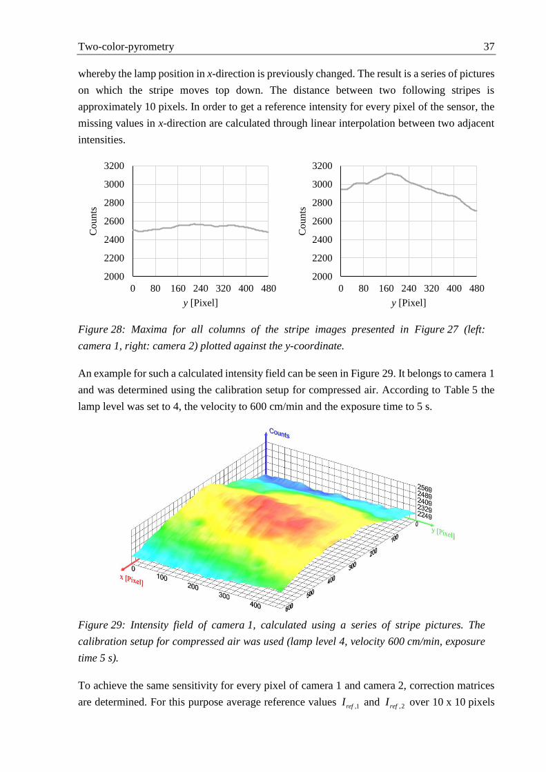
Two-color-pyrometry 37
whereby the lamp position in x-direction is previously changed. The result is a series of pictures
on which the stripe moves top down. The distance between two following stripes is
approximately 10 pixels. In order to get a reference intensity for every pixel of the sensor, the
missing values in x-direction are calculated through linear interpolation between two adjacent
intensities.
An example for such a calculated intensity field can be seen in Figure 29. It belongs to camera 1
and was determined using the calibration setup for compressed air. According to Table 5 the
lamp level was set to 4, the velocity to 600 cm/min and the exposure time to 5 s.
To achieve the same sensitivity for every pixel of camera 1 and camera 2, correction matrices
are determined. For this purpose average reference values ,1refI and ,2refI over 10 x 10 pixels
2000
2200
2400
2600
2800
3000
3200
0 80 160 240 320 400 480
Co
un
ts
y [Pixel]
2000
2200
2400
2600
2800
3000
3200
0 80 160 240 320 400 480
Counts
y [Pixel]
Figure 28: Maxima for all columns of the stripe images presented in Figure 27 (left:
camera 1, right: camera 2) plotted against the y-coordinate.
Figure 29: Intensity field of camera 1, calculated using a series of stripe pictures. The
calibration setup for compressed air was used (lamp level 4, velocity 600 cm/min, exposure
time 5 s).

38 Two-color-pyrometry
located in the middle of the intensity fields are calculated and subsequently the value of every
pixel is divided by the corresponding reference value (camera 1: ,1refI and camera 2: ,2refI ). In
Figure 30 the correction factor matrix for camera 1 calculated using the intensity field in
Figure 29 is presented. The intensity fields and the corresponding correction factor fields for
camera 2 and for the two-color-pyrometer setup used for nitrogen are shown in the
Appendix A.1.
Because of the per-element multiplication of the raw images by the correction factor matrices
before the temperature determination, it is sufficient to calculate a single calibration factor K
that is valid for the complete quotient image (see Chapter 2.2.4). For this purpose Equation 2.30
has to be solved for K , and T has to be set to refT according to the used calibration level (see
Table 4). Furthermore refQ T is given by the ratio of ,1refI and ,2refI . The final expression for
the determination of the calibration factor is summed up in Equation 2.40.
2 /
2 2 2 2,1 2 /
2 /
,21 1 1 1
2 /
,
,
FWHM
e sref i FWHM
FWHM
refe s
i FWHM
q i f i M i TI
KI
q i f i M i T
2.40
In Table 6 the calibration factors for the two-color-pyrometer setups used for compressed air
and nitrogen are listed.
Atomizing gas Level Calibration factor K [m²/W]
Compressed air 4 0.1828
Nitrogen 1 0.1236
Figure 30: Correction factors for camera 1, calculated using the intensity field in Figure 29
and the average intensity ,1refI located in the middle of the intensity field.
Table 6: Calculated calibration factors for the compressed air setup and the nitrogen setup.

Tomographic measurement of the temperature distribution 39
3 Tomographic measurement of the temperature distribution
In order to obtain a 3D temperature distribution of the spray plume, the two-color-pyrometer
has to be combined with a tomographic recording and evaluation technique. The fundamentals
of tomography and the technical realization, including the experimental setup and the data
processing, are explained in the following chapters. Furthermore the requirements on the wire
arc spray plume, that have to be fulfilled to enable tomographic investigations, are discussed.
For convenience the fundamentals of tomography are discussed on the basis of a single cross
section of the measurement object.
3.1 Fundamentals of tomography
The aim of tomography is the reconstruction of three dimensional objects using
two-dimensional distributions of measured values acquired from different directions. The
foundations for tomography were laid by the mathematician Johann Radon in 1917 with the
Radon-Transformation [116, 117]. With his work [118] he proved the existence of a projection
value ,p i that can be calculated through integrating a function ,f x y along a straight line
,iL . As long as ,f x y is steady and becomes zero within a circle with endless radius it
follows:
,
, ,
iL
p i f x y ds
3.1
As illustrated in Figure 31, ,iL is defined by the angle between the straight line and the
x -axis and the distance i to the center point.
For the generation of the projection values two different acquisition methods that depend on
the properties of the observed object, can be used. The first one, that is well-known from
Computed Tomography (CT) in human medicine, is the so called transmission tomography (see
Figure 32 left). Here the object is illuminated with an X-ray source and the transmitted light is
projected onto a detector [116]. In contrast, for emission tomography no additional light source
Figure 31: Principle of the Radon-transformation: Calculation of a value p through
integrating a function f(x,y) along a straight line given by the angle and the distance i.

40 Tomographic measurement of the temperature distribution
is necessary. The precondition for this is an object that is luminous and optically thin. A
schematic drawing of such an object is shown in Figure 32 on the right side. Optically thin
means that light emitted from any place can leave the object without being absorbed [119, 120]
and consequently information of the whole object receives the detector. Since the particles are
luminous and the radiation carries the temperature information, only emission tomography can
be considered for the wire arc spray process. The optical depth of the spray plume is discussed
in Chapter 3.2.
To be able to solve the inverse problem of Equation 3.1 and to compute ,f x y , many
projections from different directions are necessary (see Figure 33).
For this reason the detector has to be moved around the object and an image has to be acquired
in every angle step . To avoid recording of redundant information, the last measurement
position should be at an angle of 180 . Consequently the number of projection directions
k is given by Equation 3.2:
Figure 32: Principle methods for the tomographic projection generation. Left: object is
illuminated and the transmitted light is projected onto the detector. Right: optically thin and
luminous objects can be projected onto the detector without external light source.
Figure 33: Tomographic acquisition technique: The detector has to be moved around the
object and images have to be recorded in defined angle steps.

Tomographic measurement of the temperature distribution 41
180
k
3.2
Since the used detector (CCD-Sensor) measures discrete spatial values (pixels), it is obvious to
divide the cross section into cells, too. Figure 34 shows the discretization of the projections and
the cross section, including all variables and parameters necessary to describe the mathematical
problem.
Figure 34: Discretization of the projections and the cross section including all necessary
variables and parameters for the mathematical description of the inverse reconstruction
problem.

42 Tomographic measurement of the temperature distribution
To discretize the function ,f x y a quadratic grid with an edge length of n cells is applied.
The 2N n resulting values nf are used to calculate the M k n projection values
ip , which
number depends on the projection direction number l (l ll ) and the edge length n of the
quadratic grid. For the determination of ip all sub-areas of the cells, that relate to the
corresponding beam (blue lines in Figure 34), have to be taken into account. Therefore for every
projection i the N weights ,i jw have to be known. They can be calculated using Equation 3.3
,
sub-area of cell relating to projection
area of cell i j
j iw
j 3.3
As an example the weight 5,6lnw is marked green in Figure 34. An detailed description for the
systematic calculation of the weights is given in [121]. The value of a single projection value
can finally be determined with Equation 3.4.
,
1
for 1N
i i j j
j
p w f i M
3.4
By summarizing the M projections to the column vector
T
1, , Mp p p 3.5
the N values jf to the column vector
T
1, , Nf f f 3.6
and the weights to the M N matrix
1,1 1,
,1 ,
N
M M N
w w
w w
W 3.7
the set of linear equations (see Equation 3.4) can be expressed as presented in Equation 3.8:
with , and M M N N
p f
p f
W
W 3.8
Tomographic measurement of the temperature distribution 43
Since the aim of tomography is the reconstruction of the cross section and the distribution
,f x y , respectively, Equation 3.8 has to be solved for the vector f . The direct solution is
only possible if M N and if the inverse of W exists. But even if this conditions are fulfilled,
the resolution of the cross section is usually high and consequently W is large so that the direct
inversion places high demands on the processing power of computers [116]. Because of these
reasons, iterative methods are used to calculate the vector f . In this work the so called
algebraic reconstruction technique (ART) is applied to solve the tomographic problem. This
iterative ART is based on the Kaczmarz’s method [122] and can be written as follows:
11 T
Tfor 1
mm m i i
i
i i
w f pf f w i M
w w
3.9
The derivation of this equation is well defined in [116]. In every iteration step m the previous
cross section values 1m
f
are corrected -timesM using the projections ip and the
corresponding rows iw of the weight matrix W . The structure of the vector
iw is presented in
Equation 3.10.
,1 ,2 ,, , ,i i i i Nw w w w 3.10
Through applying the iterative ART it became possible to reconstruct cross sections with high
resolution and satisfactory convergence after a few iterations. The relatively fast convergence
of the algorithm could only be achieved by rearrangement of the projection indices i in one
iteration step m . It is well known in literature [123] that large angles between projections used
for the ART are good for the performance of the algorithm. Exemplary results for the
convergence are shown in Chapter 3.3.2.
As already mentioned at the beginning of this chapter the mathematical fundamentals of
tomography are only explained for the reconstruction of a single cross section using one column
of the CCD-sensor. But through stacking the cross sections calculated for all columns, a 3D-
distribution of the observed object can be created.
3.2 Properties of the wire arc spray plume regarding tomography
The tomographic two-color-pyrometry presented in this work is developed to determine three
dimensional intensity and particle temperature distributions of the wire arc spray plume.
Therefore long exposure times are necessary to guarantee a sufficiently high number of particles
on every position of the spray plume. The resulting images (see Figure 40) are very smooth and
can be used for the tomographic reconstruction.
44 Tomographic measurement of the temperature distribution
As mentioned in the previous chapter tomography is usually performed by screening an object
with an X-ray source and measuring the percentage that is not absorbed. Another way to do
tomography is the so called emission tomography. To be able to apply this method the observed
object has to be luminous and optically thin. Plasma jets for example used for thermal spraying
fulfill these requirements and have successfully been investigated using optical emission
tomography. Landes et al. [76] for example proved the triple symmetry of a “TRIPLEX II”
torch and Hlína et al. [75] calculated time resolved three dimensional plasma temperature
distributions.
In this work the measurement object is the spray plume of the wire arc spray process and the
fast moving particles, respectively. Since the particles are molten steel droplets, they are opaque
and only the light emitted from the surface can be measured. Remedy for this problem is
provided by observing no single particles but an ensemble of particles. By integrating over a
long time (>1 s) it should be guaranteed that a sufficient number of particles flies through every
point of the measurement volume so that the acquired smooth 2D images reflect statistical
particle distributions.
In addition it is necessary that the light emitted from the particles receives the detector without
being shadowed by other particles. To be able to prove this condition the parameter optical
thickness can be introduced. This dimensionless quantity is usually used to express the
radiation losses in a medium. According to [124] the relation between the source intensity totI
and the received intensity recI can be written as follows:
rec totI I e 3.11
In the case of the particle plume totI is the radiation of all particles sent to the detector and
recI
is the radiation that is received by the detector. To be able to do tomographic reconstructions
the wire arc spray plume has to be optically thin ( 1 [119, 120]).
For the determination of , spatially resolved particle rates measured by Laser Doppler
Anemometry, mean particle velocities measured by the DPV and mean particle sizes measured
by Particle Shape Imaging are used. Figure 35 for example shows a particle rate cross section
of the spray plume located 70 mm in front of the wire tips. The process parameters were set to
28.9 V, 4 m/min and 4 bar. Compressed air was used as atomizing gas.
An observation channel divided into equal-sized cubes is used in order to estimate the amount
of shadowed particles. In Figure 35 an example for such a channel is marked (white squares)
and in Figure 36 above three of these cubes and the transiting particles are enlarged in a
principle drawing. With the help of the spatially-resolved particle rates, the total number of
particles per second /ndN dt flying through the area of the n th white square in z -direction
can be calculated. As shown in Figure 36 above it is assumed that all particles go through the

Tomographic measurement of the temperature distribution 45
cubes one after the other and consequently the time ,P nt between two following particles for
channel n can be calculated as follows:
1
,n
P n
dNt
dt
3.12
Since the particle velocity variation in the xy-plane is negligible and the particle size cannot be
measured spatially-resolved, it is assumed that all particles have the same velocity Pv and the
same radius Pr . Furthermore only the velocity in z -direction ,P zv can be measured using the
DPV and consequently ,P xv and ,P yv have to be negligible, too.
The timing of the particle movement is presented in Figure 36 below. The diagram shows a
time line for every cube presented in Figure 36 above. Whereby a high pulse, whose length Pt
is given by Equation 3.13, represents the appearance of a particle.
,
2 PP
P z
rt
v 3.13
The dashed frame marked in the diagram shows the observation window. Its length is given by
the duration of stay of the particles in the cubes and can be calculated by Equation 3.14 using
the cube edge length Cl and the particle velocity ,P zv .
Figure 35: Spatially resolved particle rates measured by Laser Doppler Anemometry (see
Chapter 5.4). Cross section of the spray plume located 70 mm in front of the wire tips.
Process parameters: 28.9 V, 4 m/min, 4 bar and compressed air.

46 Tomographic measurement of the temperature distribution
,
CC
P z
lt
v 3.14
By moving the time lines with small time steps t through the stationary observation window,
the total emitted intensity totI can be calculated and the probably absorbed intensity absI can
be estimated. It has to be taken into account that all particles located in previous cubes and all
particles located in the same cube overlap the actual observed particle with a certain probability.
This probability may be expressed by Equation 3.15.
2
2
PPC
C
rL
l
3.15
Figure 36: Above: Principle drawing of three cubes taken of the observation channel and the
corresponding transiting particles. Below: Temporal connections of the transiting particles
illustrated in a diagram with marked observation window (dashed frame).

Tomographic measurement of the temperature distribution 47
The factor PCL describes the percentage of the observation channel side that is shadowed by a
particle with the radius Pr .
For the example presented in Figure 36 the total intensity of the particles located in the
observation channel is given by 06totI I and the absorbed intensity can be calculated as
follows:
0 0 0 0
1st particle in green cube 2nd p. in green cube 1st p. in red cube 3rd p. in red cube
2 3 5abs PC PC PC PCI L I L I L I L I 3.16
Since it is assumed that all particles in one cross section of the spray plume have the same
temperature and emissivity, the intensity emitted by all of them is equal and can be expressed
with 0I . Finally the optical thickness can be determined through calculating the received
intensity recI and solving Equation 3.11 for :
ln tot
tot abs
I
I I
3.17
The principle structure of the implemented algorithm is illustrated with the help of the program
flow chart in Figure 120 (Appendix A.2). As it can be seen in Figure 37 the algorithm converges
and the resulting optical depth is independent of the chosen edge length of the observation
channel cubes. Detailed results are presented in Chapter 6.5 and are discussed in Chapter 7.
0
0.02
0.04
0.06
0.08
0.1
0.12
0 0.0001 0.0002 0.0003 0.0004 0.0005
τ
t [s]
lc=0.5 mm lc=0.75 mm lc=0.96 mm lc=1.5 mmlC=0.5 mm lC=0.75 mm lC=0.96 mm lC=1.5 mm
Figure 37: Optical depths calculated using the developed algorithm and the LDA results
shown in Figure 35. The observation channel is located at x=0 and its edge length is varied.

48 Tomographic measurement of the temperature distribution
3.3 Technical realization
To be able to apply the tomographic evaluation technique presented in Chapter 3.1, an adequate
experimental setup is required for the acquisition of the raw data. Furthermore these images
have to be pre-processed in order to calculate three dimensional intensity distributions and in
the next step three dimensional temperature distributions. In the following chapters the
experimental setup and the complete data processing are explained in detail.
3.3.1 Experimental setup
A CAD-drawing of the experimental setup used for the tomographic image acquisition is
presented in Figure 38. The two-color-pyrometer module described in Chapter 2.2 is mounted
onto a rotating disk using an optical rail to extant the object distance to 625 mm. The rotation
of the ball bearing mounted disk is enabled by a mechanism consisting of a gear while, a shaft
and a stepper motor. The spray gun has to be located in such a way that the particles fly through
the whole in the middle of the disk and the gear wheel.
Figure 38: CAD-drawing of the experimental setup used for the tomographic measurements.
The setup consists of a TCP-Module mounted onto a rotating disk via an optical rail. The
disk is driven by a mechanism consisting of a gear wheel, a shaft and a stepper motor. The
wire arc gun is positioned in such a way, that the spray plume goes through the whole in the
middle of the rotating disk.
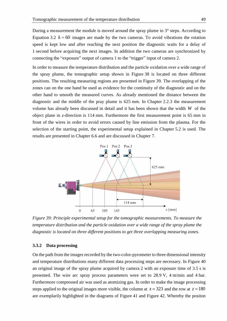
Tomographic measurement of the temperature distribution 49
During a measurement the module is moved around the spray plume in 3° steps. According to
Equation 3.2 60k images are made by the two cameras. To avoid vibrations the rotation
speed is kept low and after reaching the next position the diagnostic waits for a delay of
1 second before acquiring the next images. In addition the two cameras are synchronized by
connecting the “exposure” output of camera 1 to the “trigger” input of camera 2.
In order to measure the temperature distribution and the particle oxidation over a wide range of
the spray plume, the tomographic setup shown in Figure 38 is located on three different
positions. The resulting measuring regions are presented in Figure 39. The overlapping of the
zones can on the one hand be used as evidence for the continuity of the diagnostic and on the
other hand to smooth the measured curves. As already mentioned the distance between the
diagnostic and the middle of the pray plume is 625 mm. In Chapter 2.2.3 the measurement
volume has already been discussed in detail and it has been shown that the width W of the
object plane in z-direction is 114 mm. Furthermore the first measurement point is 65 mm in
front of the wires in order to avoid errors caused by line emission from the plasma. For the
selection of the starting point, the experimental setup explained in Chapter 5.2 is used. The
results are presented in Chapter 6.6 and are discussed in Chapter 7.
3.3.2 Data processing
On the path from the images recorded by the two-color-pyrometer to three dimensional intensity
and temperature distributions many different data processing steps are necessary. In Figure 40
an original image of the spray plume acquired by camera 2 with an exposure time of 3.5 s is
presented. The wire arc spray process parameters were set to 28.9 V, 4 m/min and 4 bar.
Furthermore compressed air was used as atomizing gas. In order to make the image processing
steps applied to the original images more visible, the column at 323x and the row at 180z
are exemplarily highlighted in the diagrams of Figure 41 and Figure 42. Whereby the positon
Figure 39: Principle experimental setup for the tomographic measurements. To measure the
temperature distribution and the particle oxidation over a wide range of the spray plume the
diagnostic is located on three different positions to get three overlapping measuring zones.

50 Tomographic measurement of the temperature distribution
323x is chosen because it is the middle of the spray plume, and 180z because of the hot
pixel that is present in this row.
The first image processing step is the convolution of the original images by a 3 3 median
filter [125], in order to remove the hot pixels and to reduce the noise. As it can be seen with the
aid of the orange trace in Figure 42, the peak (hot pixel) in the gray signal is successfully
removed using the median filter. Another filter that is used to smooth the pictures is a 3 3
mean filter [125]. Due to this filter the processed traces have significantly reduced signal noise
and can finally be multiplied pixel per pixel with the corresponding correction factor matrix
(see Chapter 2.2.5). The effect of the correction factor matrix is most in evidence comparing
the original and the processed curves in Figure 41. The processed trace is amplified from
approximately 0z to 80 and from approximately 240z to 480, in between the values are
scaled down. In the last step a 50 Pixel wide stripe is added to the upper and the lower border
of the original images, whereby the intensity of the pixels in a single row of the stripe is equal
to the mean value of the neighboring 10 pixels in the processed image. The extension to a
resolution of 740 480 is necessary, in order to be able to choose a region of sufficient range
for the tomographic reconstruction.
Figure 40: Original image of the spray plume acquired by camera 2 of the
two-color-pyrometer with an exposure time of 3.5 s. The process parameters were set to
28.9 V, 4 m/min and 4 bar. Compressed air was used as atomizing gas.
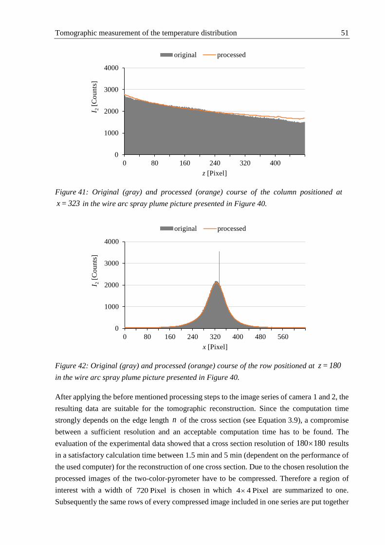
Tomographic measurement of the temperature distribution 51
After applying the before mentioned processing steps to the image series of camera 1 and 2, the
resulting data are suitable for the tomographic reconstruction. Since the computation time
strongly depends on the edge length n of the cross section (see Equation 3.9), a compromise
between a sufficient resolution and an acceptable computation time has to be found. The
evaluation of the experimental data showed that a cross section resolution of 180 180 results
in a satisfactory calculation time between 1.5 min and 5 min (dependent on the performance of
the used computer) for the reconstruction of one cross section. Due to the chosen resolution the
processed images of the two-color-pyrometer have to be compressed. Therefore a region of
interest with a width of 720 Pixel is chosen in which 4 4 Pixel are summarized to one.
Subsequently the same rows of every compressed image included in one series are put together
0
1000
2000
3000
4000
0 80 160 240 320 400
I 2[C
ou
nts
]
z [Pixel]
original processed
0
1000
2000
3000
4000
0 80 160 240 320 400 480 560
I 2[C
ou
nts
]
x [Pixel]
original processed
Figure 41: Original (gray) and processed (orange) course of the column positioned at
x = 323 in the wire arc spray plume picture presented in Figure 40.
Figure 42: Original (gray) and processed (orange) course of the row positioned at z = 180
in the wire arc spray plume picture presented in Figure 40.

52 Tomographic measurement of the temperature distribution
in a new picture. An example for such an image is presented on the left side of Figure 43. It
contains the projection values in the Cartesian Radon space [116] dependent on the index i and
the projection angle l . Before the projection values can be used for the tomographic
reconstruction additional processing steps have to be applied. At first the projection images are
blurred using a 3 3 mean filter, second a correction of the rotation axis is performed [126]
and finally the intensities in every row are scaled so that every row total is equal. The last step
is necessary because of the sequential acquisition of the images and the spray plume fluctuations
that may consequently be recorded.
With the projection values and the weights calculated according to [121] all values are available
to calculate the cross sections using Equation 3.9. Figure 43 for example shows the cross
section resulting from the projection image besides, and Figure 44 shows the development of
the intensity 2I located in the middle of this cross section. It can clearly be seen that the value
converges and does not significantly change after the 6th iteration. To guarantee the
convergence even in the fringes of the cross section the number of iterations was set to 10.
Furthermore the diagram in Figure 44 shows that in the case of this reconstruction the
computation lasted approximately 3 min.
Finally with the help of the cross section of camera 2 presented in Figure 43, the corresponding
cross section of camera 1 and the calculated quotients (Figure 21), the temperature image can
be determined. Therefore the cross section of camera 1 has to be divided pixel per pixel by the
cross section of camera 2 and the resulting quotients have to be compared with the calculated
ones. In Figure 45 the temperature image is presented, whereby the scale determined
experimentally using a ruler is used in order to get the dimensions in mm. The temperature
Figure 43: Projection values in the Cartesian Radon space and the corresponding calculated
cross section in the Cartesian space. The projections are taken from the same image series
as the original picture in Figure 40.
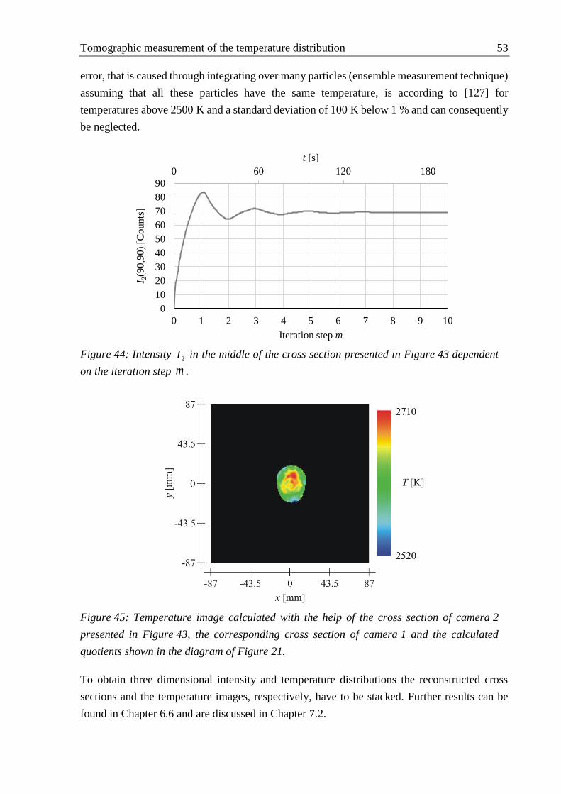
Tomographic measurement of the temperature distribution 53
error, that is caused through integrating over many particles (ensemble measurement technique)
assuming that all these particles have the same temperature, is according to [127] for
temperatures above 2500 K and a standard deviation of 100 K below 1 % and can consequently
be neglected.
To obtain three dimensional intensity and temperature distributions the reconstructed cross
sections and the temperature images, respectively, have to be stacked. Further results can be
found in Chapter 6.6 and are discussed in Chapter 7.2.
0 60 120 180
0
10
20
30
40
50
60
70
80
90
0 1 2 3 4 5 6 7 8 9 10
t [s]
I 2(9
0,9
0)
[Coun
ts]
Iteration step m
Figure 44: Intensity 2I in the middle of the cross section presented in Figure 43 dependent
on the iteration step m .
Figure 45: Temperature image calculated with the help of the cross section of camera 2
presented in Figure 43, the corresponding cross section of camera 1 and the calculated
quotients shown in the diagram of Figure 21.

54 In situ particle oxidation measurement
4 In situ particle oxidation measurement
The aim of this work is the development of a diagnostic allowing quantitative conclusions on
the particle oxidation along the spraying direction. On the basis of the three dimensional
intensity and temperature distributions measured by tomographic pyrometry, the estimation of
emissivities depending on the oxidation is performed. In the following sections brief
descriptions of the oxidation mechanism of steel and the resulting optical properties are given.
And finally within this framework the principle of oxidation measurement is explained.
4.1 Oxidation of metal particles
Since the used feedstock material is mild steel and consists to 97.493 % [91] of iron, it may be
justifiable to explain the particle oxidation behavior and the resulting optical properties by
means of iron. On the one hand this has the advantage that chemical reactions of materials
consisting of only one element are easier to handle and on the other hand that there is a lot of
research concerning the high temperature oxidation of pure metals and iron, respectively. As
the iron-oxygen phase diagram in Figure 46 [128] shows, iron above 570 °C exposed to oxygen
forms a multi-layer oxide scale consisting of FeO (Wustite), 3 4Fe O (Magnetite) and
2 3Fe O
(Haematite). Since the iron diffusion coefficient of FeO is much larger than of the other oxides
[129], the Wustite layer is predominant and much thicker [130].
Figure 46: Iron-oxygen phase diagram, showing the different oxide and iron phases
dependent on the temperature. Adopted from [128].
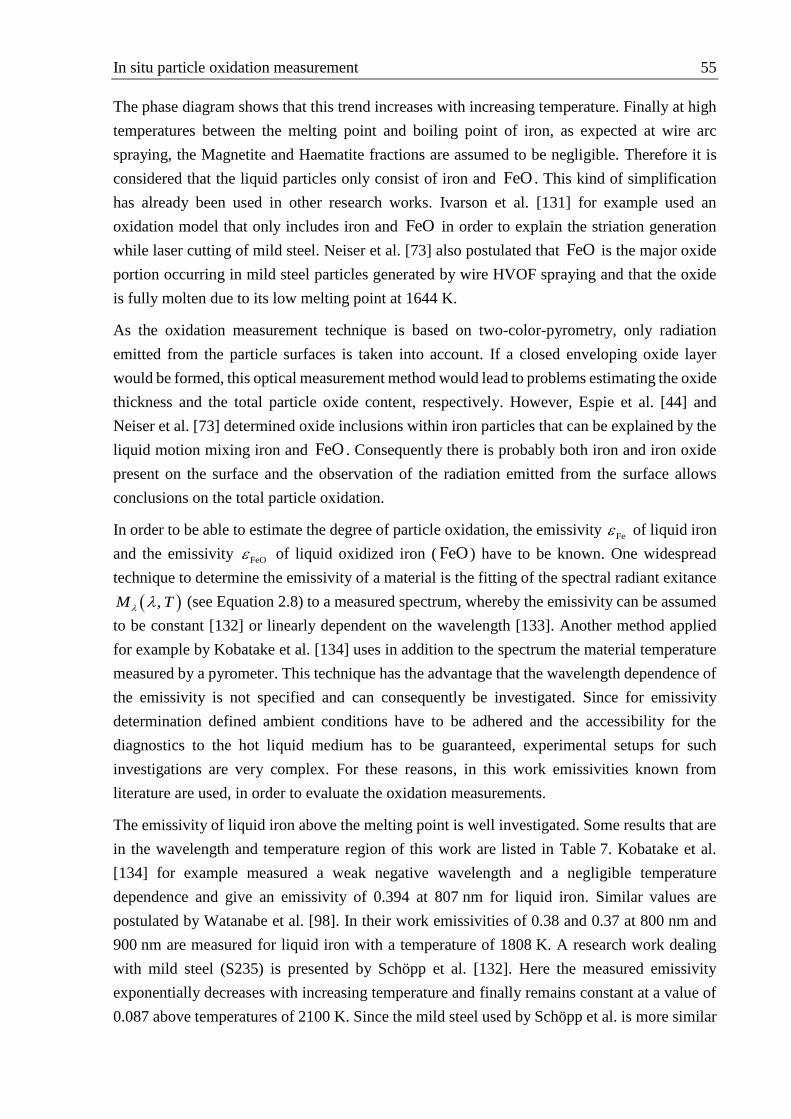
In situ particle oxidation measurement 55
The phase diagram shows that this trend increases with increasing temperature. Finally at high
temperatures between the melting point and boiling point of iron, as expected at wire arc
spraying, the Magnetite and Haematite fractions are assumed to be negligible. Therefore it is
considered that the liquid particles only consist of iron and FeO . This kind of simplification
has already been used in other research works. Ivarson et al. [131] for example used an
oxidation model that only includes iron and FeO in order to explain the striation generation
while laser cutting of mild steel. Neiser et al. [73] also postulated that FeO is the major oxide
portion occurring in mild steel particles generated by wire HVOF spraying and that the oxide
is fully molten due to its low melting point at 1644 K.
As the oxidation measurement technique is based on two-color-pyrometry, only radiation
emitted from the particle surfaces is taken into account. If a closed enveloping oxide layer
would be formed, this optical measurement method would lead to problems estimating the oxide
thickness and the total particle oxide content, respectively. However, Espie et al. [44] and
Neiser et al. [73] determined oxide inclusions within iron particles that can be explained by the
liquid motion mixing iron and FeO . Consequently there is probably both iron and iron oxide
present on the surface and the observation of the radiation emitted from the surface allows
conclusions on the total particle oxidation.
In order to be able to estimate the degree of particle oxidation, the emissivity Fe of liquid iron
and the emissivity FeO of liquid oxidized iron ( FeO ) have to be known. One widespread
technique to determine the emissivity of a material is the fitting of the spectral radiant exitance
,M T (see Equation 2.8) to a measured spectrum, whereby the emissivity can be assumed
to be constant [132] or linearly dependent on the wavelength [133]. Another method applied
for example by Kobatake et al. [134] uses in addition to the spectrum the material temperature
measured by a pyrometer. This technique has the advantage that the wavelength dependence of
the emissivity is not specified and can consequently be investigated. Since for emissivity
determination defined ambient conditions have to be adhered and the accessibility for the
diagnostics to the hot liquid medium has to be guaranteed, experimental setups for such
investigations are very complex. For these reasons, in this work emissivities known from
literature are used, in order to evaluate the oxidation measurements.
The emissivity of liquid iron above the melting point is well investigated. Some results that are
in the wavelength and temperature region of this work are listed in Table 7. Kobatake et al.
[134] for example measured a weak negative wavelength and a negligible temperature
dependence and give an emissivity of 0.394 at 807 nm for liquid iron. Similar values are
postulated by Watanabe et al. [98]. In their work emissivities of 0.38 and 0.37 at 800 nm and
900 nm are measured for liquid iron with a temperature of 1808 K. A research work dealing
with mild steel (S235) is presented by Schöpp et al. [132]. Here the measured emissivity
exponentially decreases with increasing temperature and finally remains constant at a value of
0.087 above temperatures of 2100 K. Since the mild steel used by Schöpp et al. is more similar

56 In situ particle oxidation measurement
to the mild steel used in this work than pure iron (compare Table 8 and Table 10), an emissivity
of 0.087 is assumed for the wire arc spray particles that are not oxidized.
The emissivity of oxidized metals in general is higher than the emissivity of pure metals [135].
This predication for example is proved by Muller et al. [133]. In their work they measure the
emissivity of laser molten iron in a highly oxidizing environment by means of 2D single-band
pyrometry and spectral pyrometry. For oxidized iron they determined an emissivity of
approximately 0.7 remaining constant for temperatures above 2100 K.
Apart from the different absolute values, all works listed above measured emissivities that are
independent of the temperature in the expected temperature region (>2100 K). Furthermore it
is obvious that the emissivity of liquid oxidized iron is significantly higher than the emissivity
of liquid pure iron and mild steel, respectively. For these reasons and because of the fact that
the two-color-pyrometry measures at two defined wavelengths – consequently wavelength
dependence does not matter – the determination of an emissivity increase can be interpreted as
material change due to oxidation.
Material/phase Emissivity Wavelength Temperature Reference
Iron/liquid 0.394 807 nm 1600 K to 1950 K [134]
Iron/liquid 0.38, 0.37 800 nm, 900 nm 1808 K [98]
S235/liquid 0.087 650 nm to 850 nm >2100 K [132]
FeO/liquid ~0.7 500 nm to 700 nm >2100 K [133]
Chemical element C N Mn P S Cu
Mass fraction [%] 0.17 0.012 1.4 0.035 0.035 0.55
4.2 Principle of oxidation measurement
As mentioned in the previous chapter the temperature dependence of the spectral emissivity is
negligible for the observed materials and temperature regions. Since the two-color-pyrometry
works at two defined wavelength bands and enables the temperature determination, emissivity
changes that can only accompany with material changes can be measured. For this purpose a
simplified model using the results of the tomographic two-color-pyrometry is introduced.
Figure 47 for example shows the 3D intensity reconstruction of the wire arc spray plume
Table 7: Measured emissivities of iron and oxidized iron taken from literature.
Table 8: Chemical analysis of the mild steel “S235” (material reference 1.0038) [136] used
by Schöpp et al. [132].

In situ particle oxidation measurement 57
(28.9 V, 4 m/min, 4 bar, CA) recorded using camera 1 (800 nm). For every cross section in the
xy-plane the total measured intensities 1,totI and 2,totI can be calculated with Equation 4.1
1, , , 1
1
2, , , 2
1
N
tot i C i i
i
N
tot i C i i
i
I z A t I T
I z A t I T
4.1
whereby ,iA is the luminous surface of particle i approximated by Equation 4.2, ,C it is its
dwell time in a cross section (see Equation 3.14) and 1 iI T and 2 iI T are the measured
intensities taking the optical sensitivities into account (see Equation 2.26 and 2.27).
2
PA r 4.2
Assuming that all N particles flying through a cross section have the same size, velocity,
temperature and emissivity, Equation 4.1 can be transformed to Equation 4.3.
i,
/ 1,2
,
with 2 and for 1, 2
e
s
tot C i e i s avg
s e
I z N A t z z K q f M T z d
FWHM i
4.3
Figure 47: 3D intensity reconstruction of the wire arc spray plume (28.9 V, 4 m/min, 4 bar,
compressed air) recorded using camera 1 (800 nm interfernce filter). For every cross section
total intensities 1,totI and average temperatures avgT can be calculated.

58 In situ particle oxidation measurement
In addition it is assumed that the particles are not further atomized so that their number N can
be calculated using the wire feed rate wv , the wire radius
wr , the exposure time expt of the
cameras and the particle radius Pr , whereby both wires have to be taken into account:
2
3
24
3
w exp w
P
v t rN
r
4.4
Besides the total intensities and the average temperatures measured by means of the
tomographic two-color-pyrometry, the particle diameter is measured using a PSI diagnostic (see
Chapter 5.3) and the particle velocity is measured using the DPV (see Chapter 5.4). The last
missing parameters necessary for the calculation of the emissivities are the calibration factors
1K and 2K 1 J . These parameters can be estimated by Equation 4.5 using the reference
intensities of the calibration lamp measured in Chapter 2.2.5, the edge length 0.24 mmCl of
a pixel in the image plane, the lamp velocity lampv (see Table 5) and the corresponding reference
temperatures (see Table 4). The emissivities refT of the tungsten calibration lamp are
approximated using the values determined by Watanabe et al. [98]. Therefore the mean value
between the emissivity at 800 nm and 900 nm is calculated
,
2
for 1, 2
,e
s
ref i
i
CC ref i s ref
lamp
IK i
ll T qe f M T d
v
4.5
The calibration factors for the two different setups (compressed air and nitrogen) and the
parameters used for the calculation are listed in Table 9. With the help of 1K and
2K finally the
material dependent emissivity along the spraying direction z can be determined using
Equation 4.6
,
/
,
with and for 1, 2
e
s
i tot
C i i s avg
s e i
I zz
N A t z K qe f M T z d
FWHM i
4.6
ref KT ref1 T ref2 T refT 1ref,I 2ref,I 1 1 JK 2 1 JK
2723 0.400187 0.383802 0.3919945 2561 3024 2419670716 13234368881
2190 0.41671 0.383802 0.400256 1560 3260 10811961403 87441550979
Table 9: Calibration factors 1K and
2K calculated for the compressed air setup (level 4) and
the nitrogen setup (level 1). Emissivities of tungsten are calculated according to [98].

General experimental settings and pretests 59
5 General experimental settings and pretests
To test the innovative diagnostic presented in this thesis, the wire arc spray process is chosen.
In order to evaluate the results of the diagnostic and to prove the boundary conditions, in situ
analysis of the particle plume using different diagnostics are done and test coatings are
generated. In the following chapter the general experimental settings of the process and the used
established diagnostics are presented.
5.1 Wire arc spray system
The used wire arc spray system consist of the Gas Metal Arc Welding (GMAW) power supply
“Phoenix” from the company “EWM” and the spray gun “ArcJetOne” from the company
“T-Spray”. To be able to use the power source for the wire arc spray process, it is equipped
with a second wire feeder. As usual for GMAW the power supply offers a constant voltage with
fixed wire feed rate and is direct current operating, whereby one wire serves as cathode and the
other one as anode. As described in [137] such a constant voltage supply offers a self-regulating
feature that guarantees a constant wire-workpiece distance and wire-wire distance, respectively.
In addition the mild steel wire “SW 70S G3” (material reference 1.5125) with a diameter of
1.6 mm from the company “EWM” is used as feedstock. The chemical analysis of the material
is listed in Table 10.
Chemical element C Si Mn P S
Mass fraction [%] 0.08 0.9 1.5 0.015 0.012
To achieve different particle temperatures, sizes and velocities and consequently different
particle oxidations, the most influencing parameters are varied. The investigated wire feed rates,
voltages, gas types and pressures are listed in Table 11. As already mentioned in Chapter 1.1.1
the wire arc spray process is voltage controlled and the current is proportional to the wire feed
rate.
Wire feed rate [m/min] 3, 4, 5
Voltage [V] 28.9 V, 33.0 V, 38.8
Gas Compressed air (CA), Nitrogen (N2)
Gas pressure [bar] 3, 4, 5
Base parameter 28.9 V, 4 m/min, 4 bar
Table 10: Chemical analysis of the used mild steel wire “SW 70S G3” (material reference
1.5125) from the company “ewm” [91].
Table 11: Investigated parameters of the wire arc spray process.
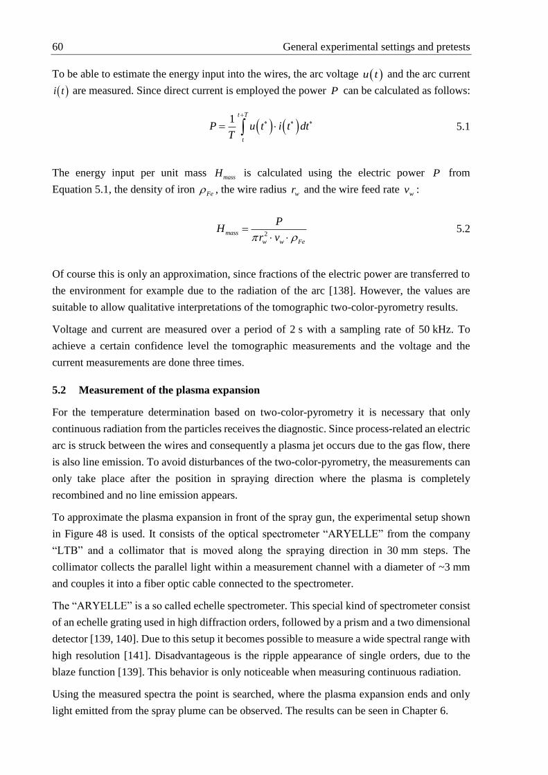
60 General experimental settings and pretests
To be able to estimate the energy input into the wires, the arc voltage u t and the arc current
i t are measured. Since direct current is employed the power P can be calculated as follows:
1
t T
t
P u t i t dtT
5.1
The energy input per unit mass massH is calculated using the electric power P from
Equation 5.1, the density of iron Fe , the wire radius
wr and the wire feed rate wv :
2mass
w w Fe
PH
r v
5.2
Of course this is only an approximation, since fractions of the electric power are transferred to
the environment for example due to the radiation of the arc [138]. However, the values are
suitable to allow qualitative interpretations of the tomographic two-color-pyrometry results.
Voltage and current are measured over a period of 2 s with a sampling rate of 50 kHz. To
achieve a certain confidence level the tomographic measurements and the voltage and the
current measurements are done three times.
5.2 Measurement of the plasma expansion
For the temperature determination based on two-color-pyrometry it is necessary that only
continuous radiation from the particles receives the diagnostic. Since process-related an electric
arc is struck between the wires and consequently a plasma jet occurs due to the gas flow, there
is also line emission. To avoid disturbances of the two-color-pyrometry, the measurements can
only take place after the position in spraying direction where the plasma is completely
recombined and no line emission appears.
To approximate the plasma expansion in front of the spray gun, the experimental setup shown
in Figure 48 is used. It consists of the optical spectrometer “ARYELLE” from the company
“LTB” and a collimator that is moved along the spraying direction in 30 mm steps. The
collimator collects the parallel light within a measurement channel with a diameter of ~3 mm
and couples it into a fiber optic cable connected to the spectrometer.
The “ARYELLE” is a so called echelle spectrometer. This special kind of spectrometer consist
of an echelle grating used in high diffraction orders, followed by a prism and a two dimensional
detector [139, 140]. Due to this setup it becomes possible to measure a wide spectral range with
high resolution [141]. Disadvantageous is the ripple appearance of single orders, due to the
blaze function [139]. This behavior is only noticeable when measuring continuous radiation.
Using the measured spectra the point is searched, where the plasma expansion ends and only
light emitted from the spray plume can be observed. The results can be seen in Chapter 6.

General experimental settings and pretests 61
5.3 Particle Shape Imaging measurements
For the oxidation approximation using the model presented in Chapter 4.2, the particle sizes
have to be known. Since the Particle Shape Imaging diagnostic enables the direct measurement
of particle sizes, it is used in this work. The experimental setup of the PSI is presented in
Figure 49. In contrast to the PSI diagnostics developed in [68, 142], a short arc lamp is used as
light source. With the help of two deflection mirrors and two lenses (focal length of 100 mm)
two light beams are focused and crossed in order to form the measurement volume. Particles
flying through the intersected area shadow the light and are projected onto an image intensifier
from different directions. The imaging optic in each optical axis consist of two lenses (focal
length of 100 mm) and three deflection mirrors. Its principle optical path without the deflection
mirrors is shown in Figure 50. Since the light of the short arc lamp covers the whole visible
spectrum, all lenses are achromatic lenses. To be able to restrict the extension of the
measurement volume an adjustable aperture is positioned in the image plane of the first lens,
which generates a one-to-one projection. By means of the second lens a magnification of
approximately six is reached. To realize the resulting long image distance the light paths are
deflected to a second plane, in which an image intensifier and a high speed camera are located.
As already mentioned in Chapter 1.1.3 the image intensifier (“Quantum Leap” from the
company “Stanford Computer Optics”) provides short exposure times at sufficient sensitivity
in order to avoid motion blur. Its principle setup and function are well described in [143] and
are not discussed further in this work. To digitalize the pictures appearing on the phosphor
screen of the image intensifier, a high-speed camera equipped with an objective is used,
whereby both devices are synchronized via the “exposure out” signal of the camera. In all
Figure 48: Experimental setup for the approximation of the plasma expansion. The setup
consist of the optical spectrometer “ARYELLE” from the company “LTB” and a collimator
that is moved along the spraying direction in 30 mm steps.
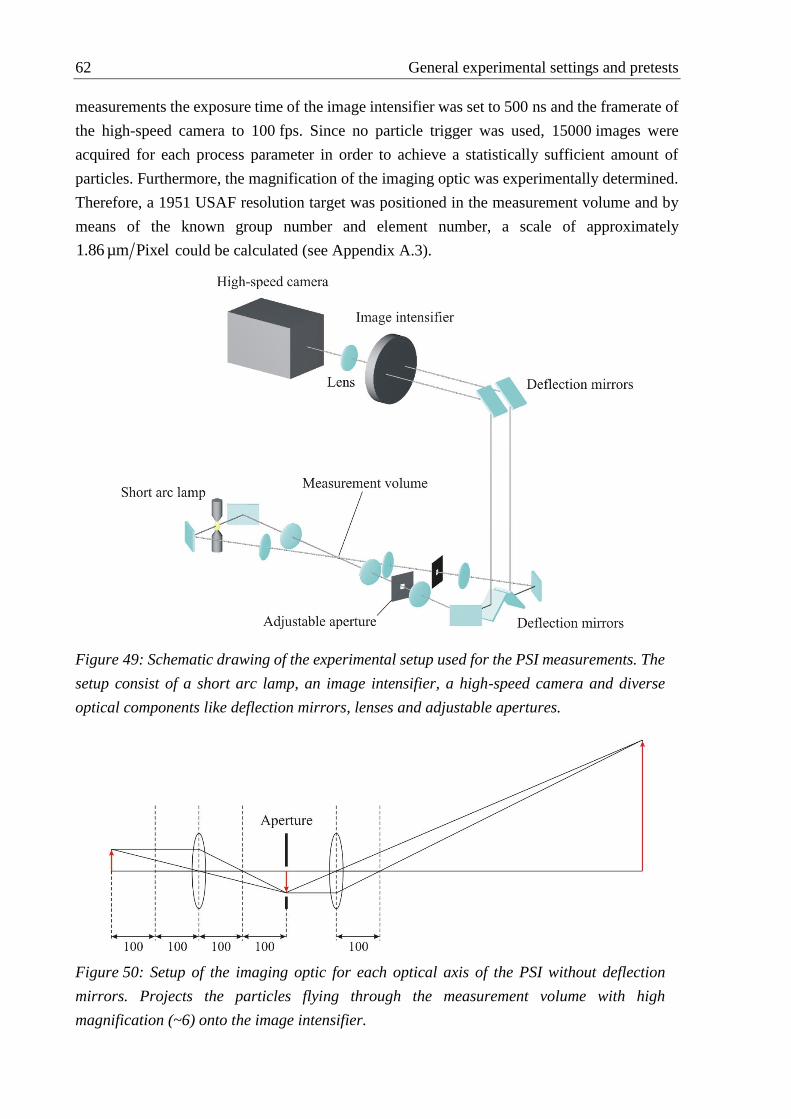
62 General experimental settings and pretests
measurements the exposure time of the image intensifier was set to 500 ns and the framerate of
the high-speed camera to 100 fps. Since no particle trigger was used, 15000 images were
acquired for each process parameter in order to achieve a statistically sufficient amount of
particles. Furthermore, the magnification of the imaging optic was experimentally determined.
Therefore, a 1951 USAF resolution target was positioned in the measurement volume and by
means of the known group number and element number, a scale of approximately
1.86 µm Pixel could be calculated (see Appendix A.3).
Figure 49: Schematic drawing of the experimental setup used for the PSI measurements. The
setup consist of a short arc lamp, an image intensifier, a high-speed camera and diverse
optical components like deflection mirrors, lenses and adjustable apertures.
Figure 50: Setup of the imaging optic for each optical axis of the PSI without deflection
mirrors. Projects the particles flying through the measurement volume with high
magnification (~6) onto the image intensifier.

General experimental settings and pretests 63
Figure 51 shows typical original images and processed images of particles flying through the
measurement volume of the PSI. Initially all images are processed the same way: a background
image is subtracted, the images are binarized using a threshold value and filtered using a median
filter, objects are searched and those contacting the frame of the region of interest (ROI) are
removed. Through comparing the size of the particles and their position in the ROI, it is proved
if both images belong to the same particle and if it is located within the measurement volume,
respectively. Since the exposure time of the image intensifier is relatively long, fast particles
(Figure 51 below) in contrast to slow particles (Figure 51 above) cause motion blur.
Consequently, the determination of the particle diameter has to be performed in two different
ways. If the vertical extension of the particles is 1.2 times larger than the horizontal extension,
the horizontal extension is used as particle diameter. If this is not the case, an area equal circle
is calculated. In addition, it is possible to determine the exact position of the particles within
the measurement volume using the relative position of a particle pair to each other and the
position within the ROI. Since only particle sizes are needed in this work, the determination of
the particle position is not discussed at this point. Figure 52 exemplarily shows particle diameter
distributions measured for compressed air at 28.9 V, 4 bar, 3 m/min and 5 m/min, respectively.
Figure 51: Original images (left) and processed images (right) of particles flying through the
measurement volume. The both images above show a slow particle the both images below a
fast particle that causes motion blur.
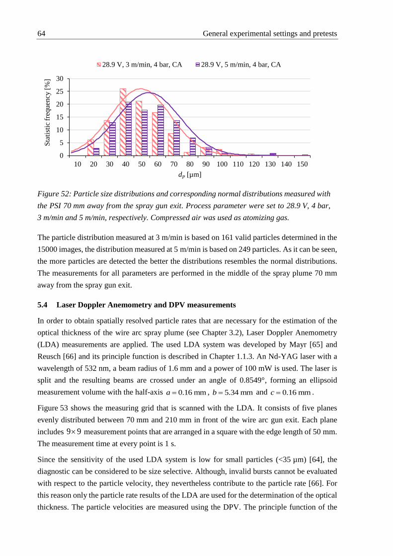
64 General experimental settings and pretests
The particle distribution measured at 3 m/min is based on 161 valid particles determined in the
15000 images, the distribution measured at 5 m/min is based on 249 particles. As it can be seen,
the more particles are detected the better the distributions resembles the normal distributions.
The measurements for all parameters are performed in the middle of the spray plume 70 mm
away from the spray gun exit.
5.4 Laser Doppler Anemometry and DPV measurements
In order to obtain spatially resolved particle rates that are necessary for the estimation of the
optical thickness of the wire arc spray plume (see Chapter 3.2), Laser Doppler Anemometry
(LDA) measurements are applied. The used LDA system was developed by Mayr [65] and
Reusch [66] and its principle function is described in Chapter 1.1.3. An Nd-YAG laser with a
wavelength of 532 nm, a beam radius of 1.6 mm and a power of 100 mW is used. The laser is
split and the resulting beams are crossed under an angle of 0.8549°, forming an ellipsoid
measurement volume with the half-axis 0.16 mma , 5.34 mmb and 0.16 mmc .
Figure 53 shows the measuring grid that is scanned with the LDA. It consists of five planes
evenly distributed between 70 mm and 210 mm in front of the wire arc gun exit. Each plane
includes 9 9 measurement points that are arranged in a square with the edge length of 50 mm.
The measurement time at every point is 1 s.
Since the sensitivity of the used LDA system is low for small particles (<35 µm) [64], the
diagnostic can be considered to be size selective. Although, invalid bursts cannot be evaluated
with respect to the particle velocity, they nevertheless contribute to the particle rate [66]. For
this reason only the particle rate results of the LDA are used for the determination of the optical
thickness. The particle velocities are measured using the DPV. The principle function of the
0 20 40 60 80 100 120 140
0
0.005
0.01
0.015
0.02
0.025
0
5
10
15
20
25
30
10 20 30 40 50 60 70 80 90 100 110 120 130 140 150
Sta
tist
ic f
requen
cy [
%]
dP [µm]
28.9 V, 3 m/min, 4 bar, CA 28.9 V, 5 m/min, 4 bar, CA
Figure 52: Particle size distributions and corresponding normal distributions measured with
the PSI 70 mm away from the spray gun exit. Process parameter were set to 28.9 V, 4 bar,
3 m/min and 5 m/min, respectively. Compressed air was used as atomizing gas.

General experimental settings and pretests 65
DPV is described in Chapter 1.1.3. Its measurement volume is positioned in the center of the
spray plume. The first measurement point is located 70 mm in front of the wire arc spray gun
exit and the following five measurement points are located downstream with a distance of
35 mm.
The results of the LDA and the DPV are used for the estimation of the optical thickness and the
calculation of the material dependent oxidation of the particles. Detailed results are presented
in Chapter 6.
5.5 Coating generation and evaluation
In order to be able to validate the tomographic oxidation measurements, test coatings are
generated and evaluated. Therefore, copper substrates are coated by moving the spray gun in
meandering shape across them (see Figure 54). The procedure is repeated six times and the
velocity of the gun is 0.67 m/s. To get several mesh points along the spraying direction the
coatings for every parameter set are produced at the distances 65 mm, 105 mm, 145 mm,
185 mm and 225 mm. For one parameter set and one distance always three substrates are coated
in order to compensate the rejects due to destruction while generating the cross sections. For
the evaluation of the coatings, scanning electron microscope (SEM) photographs (1000 times
magnification, 8 bit dynamic range) of the cross sections are used. Figure 55 a) shows a SEM
image of a coating produced with a voltage of 33 V, a wire feed rate of 4 m/min and a pressure
of 4 bar.
For the determination of the area fractions of pores, oxides and steel feedstock, several image
processing steps are applied. This method is widespread in thermal spraying and is for example
Figure 53: Measuring grid scanned with the Laser Doppler Anemometry. The grid consists
of five planes including 9 9 measurement points.
Figure 54: Meander-shaped movement of the spray gun across three copper substrates. The
test coatings are generated in order to evaluate the tomographic oxidation measurements.
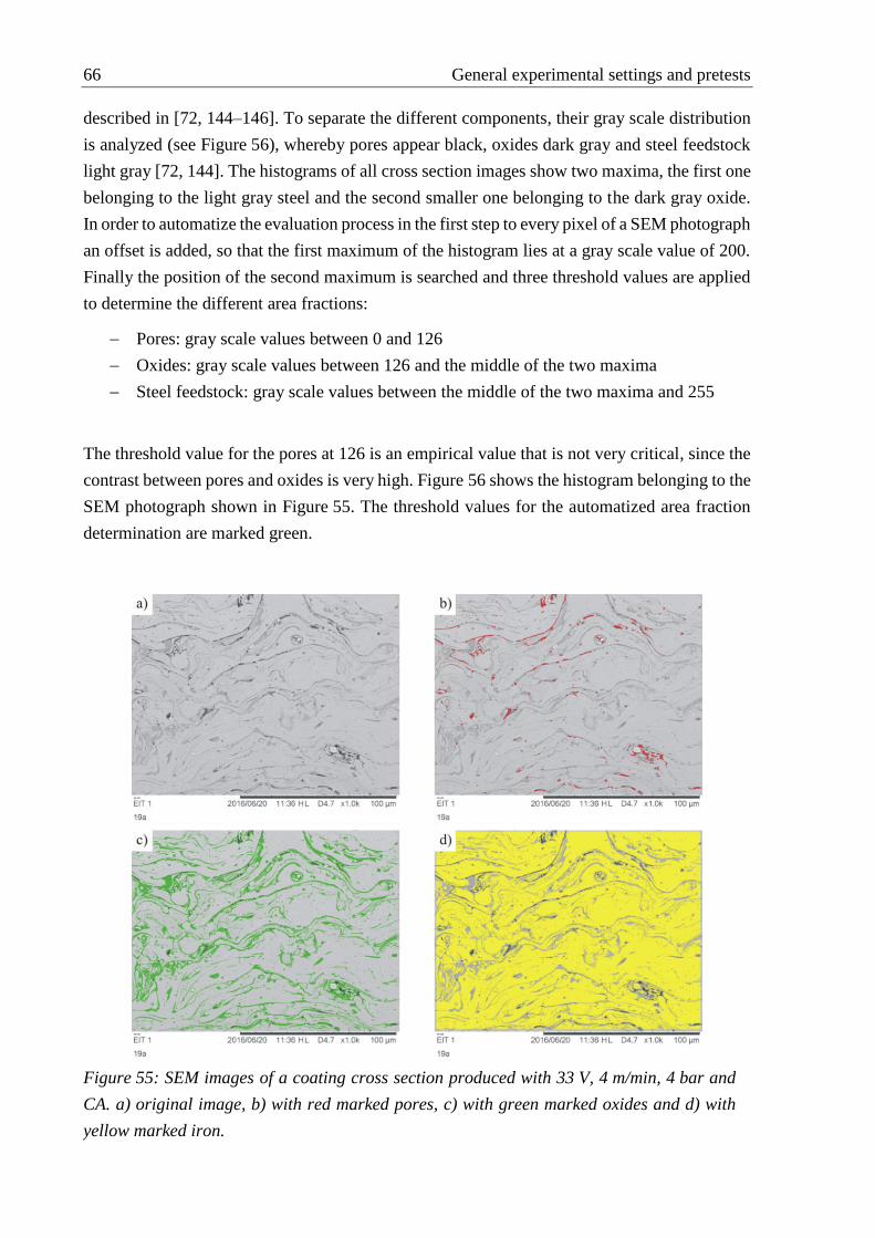
66 General experimental settings and pretests
described in [72, 144–146]. To separate the different components, their gray scale distribution
is analyzed (see Figure 56), whereby pores appear black, oxides dark gray and steel feedstock
light gray [72, 144]. The histograms of all cross section images show two maxima, the first one
belonging to the light gray steel and the second smaller one belonging to the dark gray oxide.
In order to automatize the evaluation process in the first step to every pixel of a SEM photograph
an offset is added, so that the first maximum of the histogram lies at a gray scale value of 200.
Finally the position of the second maximum is searched and three threshold values are applied
to determine the different area fractions:
Pores: gray scale values between 0 and 126
Oxides: gray scale values between 126 and the middle of the two maxima
Steel feedstock: gray scale values between the middle of the two maxima and 255
The threshold value for the pores at 126 is an empirical value that is not very critical, since the
contrast between pores and oxides is very high. Figure 56 shows the histogram belonging to the
SEM photograph shown in Figure 55. The threshold values for the automatized area fraction
determination are marked green.
Figure 55: SEM images of a coating cross section produced with 33 V, 4 m/min, 4 bar and
CA. a) original image, b) with red marked pores, c) with green marked oxides and d) with
yellow marked iron.
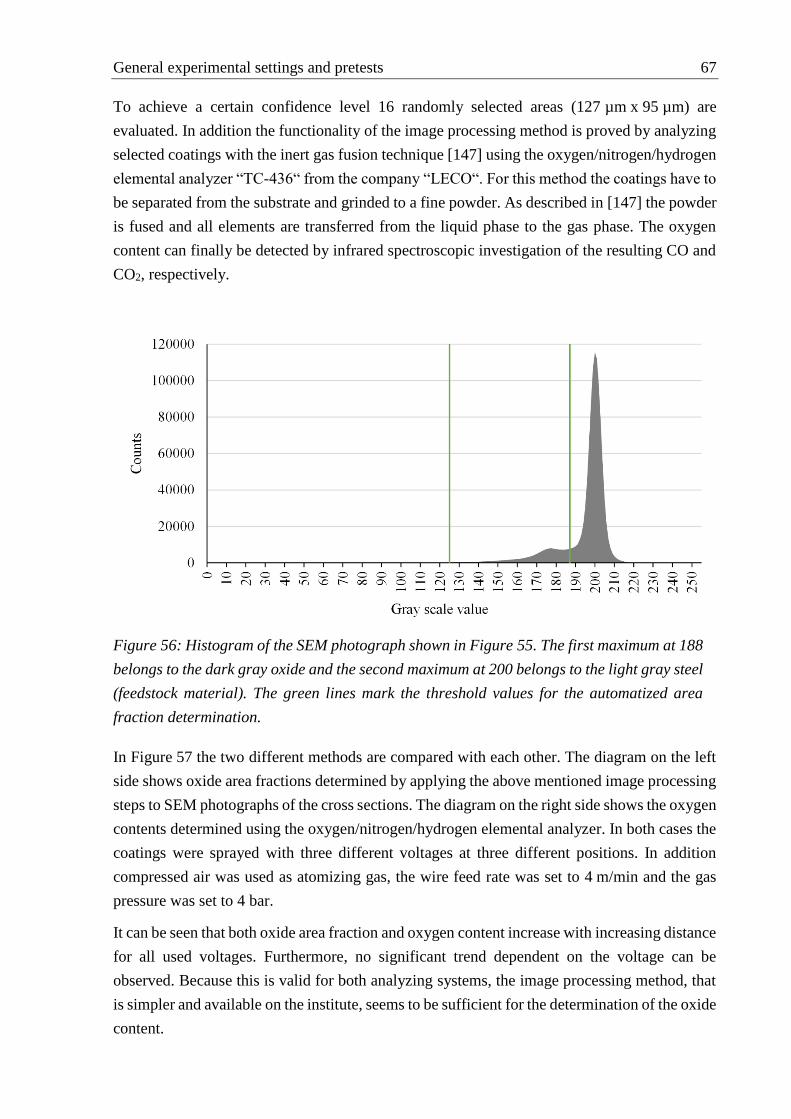
General experimental settings and pretests 67
To achieve a certain confidence level 16 randomly selected areas (127 µm x 95 µm) are
evaluated. In addition the functionality of the image processing method is proved by analyzing
selected coatings with the inert gas fusion technique [147] using the oxygen/nitrogen/hydrogen
elemental analyzer “TC-436“ from the company “LECO“. For this method the coatings have to
be separated from the substrate and grinded to a fine powder. As described in [147] the powder
is fused and all elements are transferred from the liquid phase to the gas phase. The oxygen
content can finally be detected by infrared spectroscopic investigation of the resulting CO and
CO2, respectively.
In Figure 57 the two different methods are compared with each other. The diagram on the left
side shows oxide area fractions determined by applying the above mentioned image processing
steps to SEM photographs of the cross sections. The diagram on the right side shows the oxygen
contents determined using the oxygen/nitrogen/hydrogen elemental analyzer. In both cases the
coatings were sprayed with three different voltages at three different positions. In addition
compressed air was used as atomizing gas, the wire feed rate was set to 4 m/min and the gas
pressure was set to 4 bar.
It can be seen that both oxide area fraction and oxygen content increase with increasing distance
for all used voltages. Furthermore, no significant trend dependent on the voltage can be
observed. Because this is valid for both analyzing systems, the image processing method, that
is simpler and available on the institute, seems to be sufficient for the determination of the oxide
content.
Figure 56: Histogram of the SEM photograph shown in Figure 55. The first maximum at 188
belongs to the dark gray oxide and the second maximum at 200 belongs to the light gray steel
(feedstock material). The green lines mark the threshold values for the automatized area
fraction determination.

68 General experimental settings and pretests
0
5
10
15
20
25
30
35
65 105 145
Ox
ide
area
fra
ctio
n [
%]
z [mm]
28.9 V, 4 m/min, 4 bar
33 V, 4 m/min, 4 bar
38.8 V, 4 m/min 4 bar
0
1
2
3
4
5
6
65 105 145
O2
con
ten
t [%
]
z [mm]
28.9 V, 4 m/min, 4 bar
33 V, 4 m/min, 4 bar
38.8 V, 4 m/min 4 bar
Figure 57: Left: Oxide area fractions determined using SEM photographs of cross sections.
Right: Oxygen contents determined using the oxygen/nitrogen/hydrogen elemental analyzer
“TC-436“. In both cases the coatings are sprayed with three different voltages at three
different distances. Compressed air was used as atomizing gas, the wire feed rate was set to
4 m/min and the gas pressure was set to 4 bar.
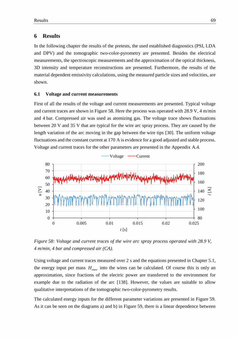
Results 69
6 Results
In the following chapter the results of the pretests, the used established diagnostics (PSI, LDA
and DPV) and the tomographic two-color-pyrometry are presented. Besides the electrical
measurements, the spectroscopic measurements and the approximation of the optical thickness,
3D intensity and temperature reconstructions are presented. Furthermore, the results of the
material dependent emissivity calculations, using the measured particle sizes and velocities, are
shown.
6.1 Voltage and current measurements
First of all the results of the voltage and current measurements are presented. Typical voltage
and current traces are shown in Figure 58. Here the process was operated with 28.9 V, 4 m/min
and 4 bar. Compressed air was used as atomizing gas. The voltage trace shows fluctuations
between 20 V and 35 V that are typical for the wire arc spray process. They are caused by the
length variation of the arc moving in the gap between the wire tips [30]. The uniform voltage
fluctuations and the constant current at 170 A is evidence for a good adjusted and stable process.
Voltage and current traces for the other parameters are presented in the Appendix A.4.
Using voltage and current traces measured over 2 s and the equations presented in Chapter 5.1,
the energy input per mass massH into the wires can be calculated. Of course this is only an
approximation, since fractions of the electric power are transferred to the environment for
example due to the radiation of the arc [138]. However, the values are suitable to allow
qualitative interpretations of the tomographic two-color-pyrometry results.
The calculated energy inputs for the different parameter variations are presented in Figure 59.
As it can be seen on the diagrams a) and b) in Figure 59, there is a linear dependence between
80
100
120
140
160
180
200
0
10
20
30
40
50
60
70
80
0 0.005 0.01 0.015 0.02 0.025
i[A
]
u[V
]
t [s]
Voltage Current
Figure 58: Voltage and current traces of the wire arc spray process operated with 28.9 V,
4 m/min, 4 bar and compressed air (CA).

70 Results
the process voltage and the heat input. This connection is valid both for compressed air and
nitrogen at a wire feed rate of 4 m/min. Changing the pressure does not affect the energy input
per mass. The results presented in Figure 59 c) measured at 28.9 V and 4 m/min show an almost
constant heat input of approximately 4750 kJ/g independent of the adjusted pressure. Finally
the influence of the wire feed rate is illustrated in Figure 59 d). An increasing wire feed rate at
28.9 V, 4 bar and compressed air leads to a decreasing energy input per mass, whereby the
relation seems to be inversely proportional.
6.2 Plasma expansion
To be sure that the recombination plasma occurring at the wire arc spray gun exit does not affect
the measurements with the tomographic two-color-pyrometry, its expansion is investigated by
means of spectroscopy. Therefore the spectrum in front of the gun is measured at different
positions using the spectrometer “ARYELLE”. Since the most electric power is implemented
4000
4500
5000
5500
6000
6500
7000
7500
25 30 35 40
Hm
ass
[J/g
]
Voltage [V]
4 m/min, 4 bar, CA
4000
4500
5000
5500
6000
6500
7000
7500
25 30 35 40
Hm
ass
[J/g
]
Voltage [V]
4 m/min, 4 bar, N2
4000
4500
5000
5500
6000
6500
7000
7500
2.5 3.5 4.5 5.5
Hm
ass
[J/g
]
Pressure [bar]
28.9 V, 4 m/min, CA
4000
4500
5000
5500
6000
6500
7000
7500
2.5 3.5 4.5 5.5
Hm
ass
[J/g
]
Feed rate [m/min]
28.9 V, 4 bar, CA
Figure 59: Energy inputs per mass calculated using the equations presented in Chapter 5.1.
a) 4 m/min, 4 bar, CA and changing voltage. b) 4 m/min, 4 bar, N2 and changing voltage. c)
28.9 V, 4 m/min, CA and changing pressure. d) 28.9 V, 4 bar, CA and changing feed rate.
a) b)
c) d)

Results 71
at high voltages and the plasma expansion is considered to be proportional to the arc power, the
spectra are measured at 38.8 V, 4 m/min and 4 bar using compressed air as atomizing gas. The
diagram in Figure 60 shows the spectra measured at three different positions along the spraying
direction. The intensity of the spectrum measured directly at the position of the wire tips (0 mm,
primary axis) is two orders of magnitude higher than the spectrum measured 30 mm in front of
the tips. Furthermore, it only shows emission lines what in turn is evidence for the presence of
plasma. The further away the measurements are performed the lower the amount of line
emission gets. At a distance of 30 mm and 60 mm the measurements between 700 nm and
900 nm only show continuous spectra coming from the thermal radiation of the particles.
Furthermore, it should be noted that the ripple appearance of the spectra originates from the
special setup of the spectrometer (see Chapter 5.2). In conclusion measurements with the
tomographic two-color-pyrometry can be applied at a distance of 60 mm without the fear of
being disturbed by line emission of the recombination plasma.
6.3 Test coatings
To be able to evaluate the in-flight particle oxidation measurements test coatings are generated
for all parameter variations at different positions along the spraying axis. In Figure 61 scanning
electron microscope (SEM) photographs of a cross section are exemplarily presented. Both
coatings were sprayed 65 mm in front of the spray gun exit with a voltage of 33 V, a feed rate
of 4 m/min and a pressure of 4 bar. For the coating on the left side compressed air was used as
atomizing gas, for the coating on the right side nitrogen. Both cross sections show the lamellar
structure, whereby the oxide content (dark gray) of the compressed air coating is significantly
higher than the oxide content of the nitrogen coating. Furthermore, the coating sprayed with
0
50
100
150
200
250
300
0
5000
10000
15000
20000
25000
30000
300 400 500 600 700 800 900
Coun
ts
Coun
ts
λ [nm]
0 mm (primary axis) 30 mm (secondary axis) 60 mm (secondary axis)
Figure 60: Spectrum of the wire arc spray process measured at different positions in front of
the wire tips using the spectrometer “ARYELLE”. The blue curve belongs to the primary axis,
the red and green curves to the secondary axis. The process parameters were set to 38.8 V,
4 m/min and 4 bar. Compressed air was used as atomizing gas.
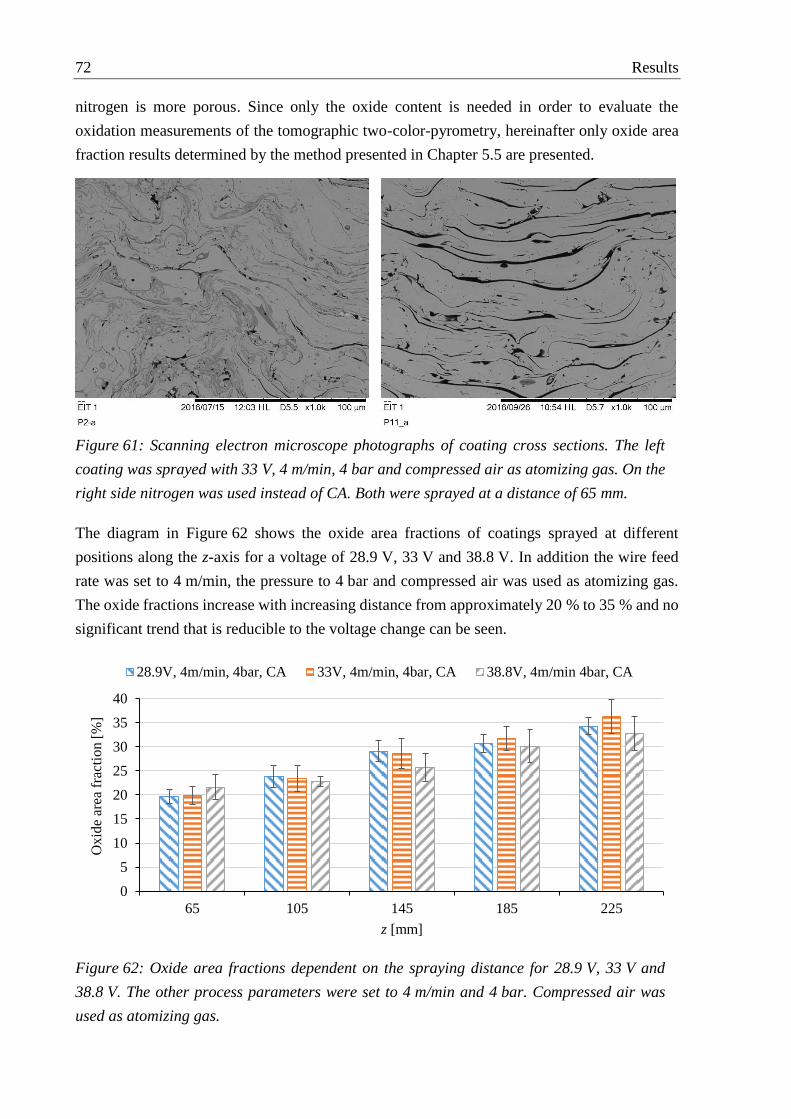
72 Results
nitrogen is more porous. Since only the oxide content is needed in order to evaluate the
oxidation measurements of the tomographic two-color-pyrometry, hereinafter only oxide area
fraction results determined by the method presented in Chapter 5.5 are presented.
The diagram in Figure 62 shows the oxide area fractions of coatings sprayed at different
positions along the z-axis for a voltage of 28.9 V, 33 V and 38.8 V. In addition the wire feed
rate was set to 4 m/min, the pressure to 4 bar and compressed air was used as atomizing gas.
The oxide fractions increase with increasing distance from approximately 20 % to 35 % and no
significant trend that is reducible to the voltage change can be seen.
0
5
10
15
20
25
30
35
40
65 105 145 185 225
Ox
ide
area
fra
ctio
n [
%]
z [mm]
28.9V, 4m/min, 4bar, CA 33V, 4m/min, 4bar, CA 38.8V, 4m/min 4bar, CA
Figure 61: Scanning electron microscope photographs of coating cross sections. The left
coating was sprayed with 33 V, 4 m/min, 4 bar and compressed air as atomizing gas. On the
right side nitrogen was used instead of CA. Both were sprayed at a distance of 65 mm.
Figure 62: Oxide area fractions dependent on the spraying distance for 28.9 V, 33 V and
38.8 V. The other process parameters were set to 4 m/min and 4 bar. Compressed air was
used as atomizing gas.
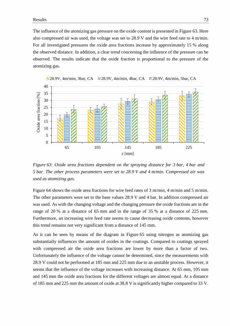
Results 73
The influence of the atomizing gas pressure on the oxide content is presented in Figure 63. Here
also compressed air was used, the voltage was set to 28.9 V and the wire feed rate to 4 m/min.
For all investigated pressures the oxide area fractions increase by approximately 15 % along
the observed distance. In addition, a clear trend concerning the influence of the pressure can be
observed. The results indicate that the oxide fraction is proportional to the pressure of the
atomizing gas.
Figure 64 shows the oxide area fractions for wire feed rates of 3 m/min, 4 m/min and 5 m/min.
The other parameters were set to the base values 28.9 V and 4 bar. In addition compressed air
was used. As with the changing voltage and the changing pressure the oxide fractions are in the
range of 20 % at a distance of 65 mm and in the range of 35 % at a distance of 225 mm.
Furthermore, an increasing wire feed rate seems to cause decreasing oxide contents, however
this trend remains not very significant from a distance of 145 mm.
As it can be seen by means of the diagram in Figure 65 using nitrogen as atomizing gas
substantially influences the amount of oxides in the coatings. Compared to coatings sprayed
with compressed air the oxide area fractions are lower by more than a factor of two.
Unfortunately the influence of the voltage cannot be determined, since the measurements with
28.9 V could not be performed at 185 mm and 225 mm due to an unstable process. However, it
seems that the influence of the voltage increases with increasing distance. At 65 mm, 105 mm
and 145 mm the oxide area fractions for the different voltages are almost equal. At a distance
of 185 mm and 225 mm the amount of oxide at 38.8 V is significantly higher compared to 33 V.
0
5
10
15
20
25
30
35
40
65 105 145 185 225
Ox
ide
area
fra
ctio
n [
%]
z [mm]
28.9V, 4m/min, 3bar, CA 28.9V, 4m/min, 4bar, CA 28.9V, 4m/min, 5bar, CA
Figure 63: Oxide area fractions dependent on the spraying distance for 3 bar, 4 bar and
5 bar. The other process parameters were set to 28.9 V and 4 m/min. Compressed air was
used as atomizing gas.

74 Results
6.4 Particle size, rate and velocity
In this chapter the results of the PSI, the LDA and the DPV measurements are presented. The
determined particle sizes, rates and velocities are used in the next two chapters in order to
approximate the optical thickness of the wire arc spray plume and to calculate the material
dependent emissivity of the particles.
0
5
10
15
20
25
30
35
40
65 105 145 185 225
Ox
ide
area
fra
ctio
n [
%]
z [mm]
28.9V, 3m/min, 4bar, CA 28.9V, 4m/min, 4bar, CA 28.9V, 5m/min, 4bar, CA
0
5
10
15
20
25
65 105 145 185 225
Ox
ide
area
fra
ctio
n [
%]
z [mm]
28.9V, 4m/min, 4bar, N₂ 33V, 4m/min, 4bar, N₂ 38.8V, 4m/min 4bar, N₂
Figure 64: Oxide area fractions dependent on the spraying distance for 3 m/min, 4 m/min
and 5 m/min. The other process parameters were set to 28.9 V and 4 bar. Compressed air
was used as atomizing gas.
Figure 65: Oxide area fractions dependent on the spraying distance for 28.9 V, 33 V and
38.8 V. The other process parameters were set to 4 m/min and 4 bar. Nitrogen was used as
atomizing gas.

Results 75
Since for all following calculations mean values of the particle radii are used, no further particle
size distributions are presented. The diagrams in Figure 66 show the mean particle sizes for the
different investigated parameter combinations. Diagram a) illustrates the influence of the
voltage, whereby compressed air was used, the feed rate was set to 4 m/min and the pressure to
4 bar. As it can be seen, the particle radius slightly increases from approximately 22 µm at
28.9 V to 22.9 µm at 33 V. Increasing the voltage to 38.8 V leads to an increased radius of
~25 µm. Using nitrogen as atomizing gas apparently does not affect the particle size. The
particle radius at 33 V, 4 m/min and 4 bar is almost equal for compressed air and nitrogen. The
measurements with nitrogen again could not be performed at all three voltage parameters, since
the process was unstable and the PSI had to be protected from unmolten wire pieces. The
influence of the pressure is presented in diagram c). Between 3 bar and 4 bar the mean particle
radius slightly decreases, whereas at a pressure of 5 bar the radius strongly decreases to ~20 µm.
19
20
21
22
23
24
25
26
25 30 35 40
r P[µ
m]
Voltage [V]
4 m/min, 4 bar, CA
19
20
21
22
23
24
25
26
25 30 35 40
r P[µ
m]
Voltage [V]
4 m/min, 4 bar, Nitrogen
19
20
21
22
23
24
25
26
2.5 3.5 4.5 5.5
r P[µ
m]
Pressure [bar]
28.9 V, 4 m/min, CA
19
20
21
22
23
24
25
26
2.5 3.5 4.5 5.5
r P[µ
m]
Feed rate [m/min]
28.9 V, 4 bar, CA
Figure 66: Particle radii measured with the Particle Shape Imaging diagnostic. a) 4 m/min,
4 bar, CA and changing voltage. b) 4 m/min, 4 bar, N2 and changing voltage. c) 28.9 V,
4 m/min, CA and changing pressure. d) 28.9 V, 4 bar, CA and changing feed rate.
a) b)
c) d)

76 Results
Diagram d) in Figure 66 shows the mean particle radii for a wire feed rate of 3 m/min, 4 m/min
and 5 m/min. The voltage was set to 28.9 V and the pressure to 4 bar. In addition compressed
air was used as atomizing gas. The results indicate that there is no clear trend between the wire
feed rate and the mean particle size. From 3 m/min to 4 m/min the radius slightly decreases,
whereas at 5 m/min the size in turn strongly declines to approximately 24.7 µm
To be able to estimate the optical thickness, particle rates were measured using the LDA. In the
following, for reasons of simplicity only 2D particle rate distributions in the xy-plane, 70 mm
in front of the wire arc spray gun exit are presented. The images in Figure 67 show the spatial
resolved particle rates measured at 28.9 V, 33 V and 38.8 V. The other parameters in turn were
set to the base parameters and compressed air was used as atomizing gas. Besides the oval
appearance of the spray plume cross sections, it can be observed that with increasing voltage
the wire arc spray plume spreads. Furthermore the maximum particle rate in the middle
increases from 28.9 V to 33 V, whereas from 33 V to 38.8 V it decreases again.
As can be seen in Figure 68, through increasing the gas pressure the spray plume gets
constricted and the maximum particle rate in the middle increases. In addition the oval form of
the cross section turns to a more round appearance. Besides the usage of compressed air, the
other parameters for these measurements were set to 4 m/min and 4 bar.
The influence of the wire feed rate is illustrated in Figure 69. With increasing wire feed rate the
maximum and the total particle rates increase. Furthermore the shape of the cross sections again
gets more round with increasing wire feed rate.
Using nitrogen instead of compressed air leads to lower particle rates and a round appearance
of the spray plume in the xy-plane. The corresponding 2D particle rates for 33 V and 38.8 V are
presented in Figure 70. The pressure was set to 4 bar, the feed rate to 4 m/min. For reasons of
comparability the space resolved particle distribution for compressed air measured at 33 V,
4 m/min and 4 bar is shown on the right side of Figure 70.
Figure 67: Particle rates for a changing voltage measured with the LDA in the xy-plane at
z=70 mm. The other parameters were set to 4 m/min, 4bar and compressed air was used.

Results 77
Figure 68: Particle rates for a changing pressure measured with the LDA in the xy-plane at
z=70 mm. The other parameters were set to 28.9 V, 4 m/min and compressed air was used.
Figure 69: Particle rates for a changing wire feed rate measured with the LDA in the xy-plane
at z=70 mm. The other parameters were set to 28.9 V, 4 bar and compressed air was used.
Figure 70: Particle rates for a changing voltage and nitrogen measured with the LDA in the
xy-plane at z=70 mm. The other parameters were set to 4 m/min and 4 bar. For comparison
the particle rate distribution for compressed air and 33 V is illustrated on the right side.

78 Results
The particle velocities measured with the DPV are necessary both for the optical thickness
calculations and for the particle emissivity determinations. To minimize the experimental
efforts the particle velocities are only measured in the middle of the spray plume on six points
along the spraying axis. Finally the particle velocity ,P zv dependent on the z-coordinate is
approximated by fitting a polynomial of third order to the measurement points.
The diagram in Figure 71 shows the particle velocities depending on the z-coordinate for a
changing voltage. The wire feed rate was set to 4 m/min and the pressure to 4 bar. In addition
compressed air was used as atomizing gas. As it can be seen, at the beginning the velocities
increase and finally from 130 mmz decrease. Furthermore at the beginning at 70 mmz
the velocities are separated from each other by about 5 m/s, whereby the velocity increases with
decreasing voltage. However, at the end the velocities are closer to each other and the influence
of the voltage is maintained when the measured value for 28.9 V at 190 mm is considered as
outlier. The polynomial fits for a voltage of 33 V and a voltage of 38.8 V have satisfactory
coefficients of determination above 0.99. At 28.9 V the coefficient is only 0.97 due to the outlier
at 190mmz .
How the diagram in Figure 72 shows, the influence of the atomizing gas pressure on the particle
velocity is significant. The velocity using 4 bar is over the whole observed distance
approximately 15 to 20 m/s higher than at a pressure of 3 bar. The difference between 4 bar and
5 bar increases from ~8 m/s at 65 mm to almost 15 m/s at 220 mm. As with the changing
vP,z = 0.00002708z3 - 0.01376485z2 + 2.05280177z + 47.54068017
R² = 0.97074337
vP,z = 0.00001345z3 - 0.00820004z2 + 1.39629705z + 65.45298330
R² = 0.99886512
vP,z = 0.00001546z3 - 0.00941131z2 + 1.62269057z + 49.75661043
R² = 0.99764244
100
110
120
130
140
150
160
65 85 105 125 145 165 185 205 225
v P,z
[m/s
]
z [mm]
28.9V, 4m/min, 4bar, CA 33V, 4m/min, 4bar, CA 38.8V, 4m/min, 4bar, CA
Figure 71: Particle velocities depending on the z-coordinate for a changing voltage and the
corresponding third order polynomial fits with its coefficients of determination. The other
parameters were set to 4 m/min, 4 bar and compressed air was used.
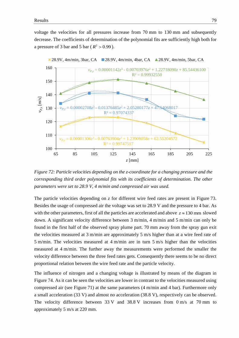
Results 79
voltage the velocities for all pressures increase from 70 mm to 130 mm and subsequently
decrease. The coefficients of determination of the polynomial fits are sufficiently high both for
a pressure of 3 bar and 5 bar ( 2 0.99R ).
The particle velocities depending on z for different wire feed rates are present in Figure 73.
Besides the usage of compressed air the voltage was set to 28.9 V and the pressure to 4 bar. As
with the other parameters, first of all the particles are accelerated and above 130 mmz slowed
down. A significant velocity difference between 3 m/min, 4 m/min and 5 m/min can only be
found in the first half of the observed spray plume part. 70 mm away from the spray gun exit
the velocities measured at 3 m/min are approximately 5 m/s higher than at a wire feed rate of
5 m/min. The velocities measured at 4 m/min are in turn 5 m/s higher than the velocities
measured at 4 m/min. The further away the measurements were performed the smaller the
velocity difference between the three feed rates gets. Consequently there seems to be no direct
proportional relation between the wire feed rate and the particle velocity.
The influence of nitrogen and a changing voltage is illustrated by means of the diagram in
Figure 74. As it can be seen the velocities are lower in contrast to the velocities measured using
compressed air (see Figure 71) at the same parameters (4 m/min and 4 bar). Furthermore only
a small acceleration (33 V) and almost no acceleration (38.8 V), respectively can be observed.
The velocity difference between 33 V and 38.8 V increases from 0 m/s at 70 mm to
approximately 5 m/s at 220 mm.
vP,z = 0.00001306z3 - 0.00763904z2 + 1.23909058z + 62.55204572
R² = 0.99747517
vP,z = 0.00002708z3 - 0.01376485z2 + 2.05280177z + 47.54068017
R² = 0.97074337
vP,z = 0.00001142z3 - 0.00703976z2 + 1.22718090z + 85.54436100
R² = 0.99932550
100
110
120
130
140
150
160
65 85 105 125 145 165 185 205 225
v P,z
[m/s
]
z [mm]
28.9V, 4m/min, 3bar, CA 28.9V, 4m/min, 4bar, CA 28.9V, 4m/min, 5bar, CA
Figure 72: Particle velocities depending on the z-coordinate for a changing pressure and the
corresponding third order polynomial fits with its coefficients of determination. The other
parameters were set to 28.9 V, 4 m/min and compressed air was used.

80 Results
vP,z = 0.00001099z3 - 0.00715255z2 + 1.26948894z + 71.44999610
R² = 0.99732338
vP,z = 0.00002708z3 - 0.01376485z2 + 2.05280177z + 47.54068017
R² = 0.97074337
vP,z = 0.00000836z3 - 0.00557333z2 + 1.02836285z + 76.74248577
R² = 0.99951213
100
110
120
130
140
150
160
65 85 105 125 145 165 185 205 225
v P,z
[m/s
]
z [mm]
28.9V, 3m/min, 4bar, CA 28.9V, 4m/min, 4bar, CA 28.9V, 5m/min, 4bar, CA
vP,z = 0.00001066z3 - 0.00561834z2 + 0.86568708z + 80.40874100
R² = 0.99459022
vP,z = 0.00000494z3 - 0.00282246z2 + 0.41985584z + 98.83269248
R² = 0.99973395
100
110
120
130
140
150
160
65 85 105 125 145 165 185 205 225
v P,z
[m/s
]
z [mm]
33V, 4m/min, 4bar, N₂ 38.8V, 4m/min, 4bar, N₂
Figure 73: Particle velocities depending on the z-coordinate for a changing wire feed rate
and the corresponding third order polynomial fits with its coefficients of determination. The
other parameters were set to 28.9 V, 4 bar and compressed air was used.
Figure 74: Particle velocities depending on the z-coordinate for a changing voltage and the
corresponding third order polynomial fits with its coefficients of determination. The other
parameters were set to 4 m/min, 4 bar and nitrogen was used.
Results 81
6.5 Optical thickness of the spray plume
For the determination of the optical thickness the 2D particle rate distributions measured with
the LDA are used (see Chapter 6.4). The example in Figure 75 shows such spatially resolved
particle rates in the xy-plane including nine observation channels located in 5 mm steps along
the x-axis. By means of these channels the optical thickness, depending on the distance to the
middle of the spray plume, is calculated using the algorithm presented in Chapter 3.2. Since the
variation of the optical thickness depending on the z-coordinate is negligible, only the LDA
results at 70 mmz are shown in the following. Furthermore the evaluation of only one
observation direction is sufficient, since the spray plume is almost rotationally symmetric.
The diagram in Figure 76 shows the optical thickness depending on x for a changing voltage.
The other parameters again are set to the base parameters, 4 m/min and 4 bar. In addition
compressed air was used as atomizing gas. The optical thickness curves for all three voltages
resemble a Gaussian distribution, whereby the maxima are located at 0 mmx . Furthermore,
increasing the voltage leads to an increasing optical thickness. The highest optical thickness of
0.045 is reached for a voltage of 38.8 V.
The results for a changing pressure, 28.9 V, 4 m/min and compressed air are presented in
Figure 77. Again the curves are similar to Gaussian distributions and the maxima belong to the
channel passing through the middle of spray plume. Increasing the pressure results in a
decreasing optical thickness. The maximum value was determined for a pressure of 3 bar and
is 0.035 .
The influence of the wire feed rate on the optical thickness is shown by means of the diagram
in Figure 78. The other parameters again were set to the base parameters. All three curves show
Figure 75: Example for a spatially resolved particle rate distribution measured with the LDA
including the nine observation channels used for the optical thickness determination.

82 Results
the typical Gaussian form with the maxima at 0 mmx . No significant trend concerning the
feed rate can be recognized, since the values for 3 m/min and 4 m/min are almost equal and the
values for 5 m/min are higher.
0.00
0.01
0.02
0.03
0.04
0.05
-25 -20 -15 -10 -5 0 5 10 15 20 25
τ
x [mm]
28.9V, 4m/min, 4bar, CA 33V, 4m/min, 4bar, CA 38.8V, 4m/min, 4bar, CA
0.00
0.01
0.02
0.03
0.04
0.05
-25 -20 -15 -10 -5 0 5 10 15 20 25
τ
x [mm]
28.9V, 4m/min, 3bar, CA 28.9V, 4m/min, 4bar, CA 28.9V, 4m/min, 5bar, CA
0.00
0.01
0.02
0.03
0.04
0.05
-25 -20 -15 -10 -5 0 5 10 15 20 25
τ
x [mm]
28.9V, 3m/min, 4bar, CA 28.9V, 4m/min, 4bar, CA 28.9V, 5m/min, 4bar, CA
Figure 76: Optical thickness at z 70 mm dependent on the x-coordinate for a changing
voltage. The other parameters were set to the base parameters (4 m/min, 4 bar, CA).
Figure 77: Optical thickness at z 70 mm dependent on the x coordinate for a changing
pressure. The other parameters were set to the base parameters (28.9 V, 4 m/min, CA).
Figure 78: Optical thickness at z 70 mm dependent on the x coordinate for a changing
wire feed rate. The other parameters were set to the base parameters (28.9 V, 4 bar, CA).

Results 83
Using nitrogen instead of compressed air does not significantly affect the optical thickness. The
curve calculated for 33 V, 4 m/min and 4 bar is presented in Figure 79. It resembles a Gaussian
distribution, whereby the maximum value of 0.027 is located at 0 mmx .
6.6 Tomographic measurements
Important results that can be achieved with the tomographic two-color-pyrometry are the
three-dimensional intensity reconstructions. Since the intensities according to Equation 4.3
depend on the particle rate, velocity, size, temperature and emissivity, the 3D reconstructions
only allow qualitative conclusions. For reasons of clarity in the following only the
reconstructions for camera 1 (800 nm) are presented. They are made up of the single
measurements at the three positions shown in Figure 39 and are presented using eight
isosurfaces and a filled contour grid plane located at 60 mmz .
For the 3D intensity distribution shown in Figure 80 the process was operated at the base
parameters. The shape of the spray plume resembles an oval cylinder with a slightly downwards
pronounced bulge. The maximum intensity was measured in the middle of the spray plume at
60 mmz . Furthermore the extension of the outer isosurface is over the whole measured
distance almost constant. How the reconstruction in Figure 81 shows, increasing the voltage to
33 V leads to a much more pronounced bulge, whereby the maximum at 60 mmz increases
and shifts upwards. The effect on the shape of the spray plume for a further increase of the
voltage to 38.8 V is presented in Figure 82. The widening of the bulge proceeds and a second
lower maximum appears below the first one, whereby the larger upper maximum is again
smaller than the maximum measured at 33 V. Finally it seems that increasing the voltage leads
to the splitting of the spray plume into an upper and a bottom part merging with increasing
distance to the wire arc gun exit.
0.00
0.01
0.02
0.03
0.04
0.05
-25 -20 -15 -10 -5 0 5 10 15 20 25
τ
x [mm]
33V, 4m/min, 4bar, N₂
Figure 79: Optical thickness at z 70 mm dependent on the x-coordinate for nitrogen, 33 V,
4 m/min and 4 bar.
84 Results
Figure 80: 3D intensity reconstruction measured with camera 1 (800 nm) at 28.9 V,
4 m/min, 4 bar and compressed air as atomizing gas.
Figure 81: 3D intensity reconstruction measured with camera 1 (800 nm) at 33 V, 4 m/min,
4 bar and compressed air as atomizing gas.
Figure 82: 3D intensity reconstruction measured with camera 1 (800 nm) at 38.8 V, 4 m/min,
4 bar and compressed air as atomizing gas.

Results 85
Hereafter the influence of the atomizing gas pressure is presented. Figure 83 shows the 3D
reconstruction of the spray plume for a pressure of 3 bar, Figure 84 the 3D reconstruction of
the spray plume for a pressure of 5 bar. For both measurements the wire feed rate was set to
4 m/min and the voltage to 28.9 V. Furthermore compressed air was used as gas. It can be seen
that the expansion of the spray plume in radial direction increases with decreasing pressure,
consequently the maximum at 3 bar ( 1,max 104I ) is much smaller than maximum at 5 bar
( 1,max 199I ). In summary it can be said that increasing the pressure leads to the constriction
of the spray plume.
Figure 83: 3D intensity reconstruction measured with camera 1 (800 nm) at 28.9 V, 4 m/min,
3 bar and compressed air as atomizing gas.
Figure 84: 3D intensity reconstruction measured with camera 1 (800 nm) at 28.9 V, 4 m/min,
5 bar and compressed air as atomizing gas.
86 Results
For the 3D intensity distributions presented in Figure 85 and Figure 86 the process was operated
with 3 m/min and 5 m/min, respectively. The other parameters again were set to the base
parameters. Comparing the results measured at 3 m/min, 4 m/min (see Figure 80) and 5 m/min
it is noticeable that the form at 60 mmz does not significantly change. All in all it remains
oval with a slightly downwards pronounced bulge. However, the expansion of the isosurfaces
increases with increasing wire feed rate, what also becomes apparent on the rising maxima.
Figure 85: 3D intensity reconstruction measured with camera 1 (800 nm) at 28.9 V, 3 m/min,
4 bar and compressed air as atomizing gas.
Figure 86: 3D intensity reconstruction measured with camera 1 (800 nm) at 28.9 V, 5 m/min,
4 bar and compressed air as atomizing gas.

Results 87
Using nitrogen instead of compressed air strongly affects the shape of the wire arc spray plume.
In Figure 87 and Figure 88 the 3D reconstructions for nitrogen measured at a voltage of 33 V
and 38.8 V are presented. Here the bulge is very pronounced and the extension of the
isosurfaces in spraying direction is comparatively low. In contrary to compressed air, increasing
the voltage causes a shift of the maximum at 60 mmz downwards. Comparing the
reconstructions for compressed air and for nitrogen it has to be taken into a count that the
maximum of the legend has been changed from 200 to 40.
Figure 87: 3D intensity reconstruction measured with camera 1 (800 nm) at 33 V, 4 m/min,
4 bar and nitrogen as atomizing gas.
Figure 88: 3D intensity reconstruction measured with camera 1 (800 nm) at 38.8 V, 4 m/min,
4 bar and nitrogen as atomizing gas.

88 Results
Besides the 3D intensity reconstructions 3D temperature distributions are calculated. A typical
temperature cross section measured in the yz-plane of the spray plume at 0 mmx for the base
parameters is presented in Figure 89. Here the temperatures range from 2500 K to 2860 K,
whereby the standard deviation is small. Due to these small temperature differences and the
inhomogeneity of the distributions, the 3D presentation of the temperature reconstructions is
not very informative. For these reasons only temperature cross sections in the xy-plane at
70 mmz are exemplarily shown. These 2D temperature images are in turn used in order to
calculate the average particle temperatures along the spraying direction necessary for the
material dependent emissivity determination.
The temperature cross sections for 28.9 V, 33 V and 38.8 V are presented in Figure 90. It can
be seen that increasing the voltage leads to an increase of the particle temperature. The average
temperature is 2663 K for a voltage of 28.9 V, 2736 K for a voltage of 33 V and 2821 K for a
voltage of 38.8 V.
Figure 91 shows the 2D temperature images at 70 mmz for a changing pressure and the base
parameters (4 m/min, 4 bar and CA). To highlight the influence of the changed parameter on
the temperature, different temperature regions for the legend are chosen. Thus it becomes clear
that with increasing pressure the temperatures decrease, whereby the difference between the
average temperatures at 3 bar ( 2676 KavgT ) and 5 bar ( 2631 KavgT ) is rather low.
As the images in Figure 92 show the particle temperatures also decrease with increasing wire
feed rate. With an average temperature of 2703 K at 3 m/min and an average temperature of
2598 K the effect again is very marked.
Figure 89: Temperature cross sections of the spray plume measured in the yz-plane at
x 0 mm for the base parameters 28.9 V, 4m/min, 4 bar and CA as gas.
Results 89
Figure 90: Temperature cross sections of the spray plume measured in the xy-plane at
z 70 mm for a changing voltage and the base parameters 4m/min, 4 bar and CA as gas.
Figure 91: Temperature cross sections of the spray plume measured in the xy-plane at
z 70 mm for a changing pressure and the base parameters 28.9 V, 4m/min and CA as gas.
Figure 92: Temperature cross sections of the spray plume measured in the xy-plane at
z 70 mm for a changing feed rate and the base parameters 29.9 V, 4 bar and CA as gas.
90 Results
Using nitrogen as atomizing gas instead of compressed air leads to lower particle temperatures.
The average temperatures of the distributions presented in Figure 93 are 2592 K for 33 V and
2722 K for 38.8 V. The trend of increasing particle temperatures with increasing voltage
remains unchanged using nitrogen.
As already mentioned in Chapter 4.2, for the calculation of the material dependent emissivities
some assumptions have to be made. First of all, it has to be assumed that all particles in the
whole measurement volume have the same particle size and are consequently not further
atomized. The used particle radii Pr measured with the PSI in the middle of the spray plume at
70 mmz and the from this calculated numbers of particles N (see Equation 4.4) are listed
in Table 12.
Parameter set m minwv expt s µmPr N
28.9 V, 4 m/min, 4 bar, CA 4 3.5 22.0 18410455
33 V, 4 m/min, 4 bar, CA 4 3.5 22.8 18410455
38.8 V, 4 m/min, 4 bar, CA 4 3.5 25.1 14336000
28.9 V, 4 m/min, 3 bar, CA 4 3.5 22.4 21036814
28.9 V, 4 m/min, 5 bar, CA 4 3.5 20.3 28000000
28.9 V, 3 m/min, 4 bar, CA 3 3.5 22.2 15777611
28.9 V, 5 m/min, 4 bar, CA 5 3.5 24.7 17920000
33 V, 4 m/min, 4 bar, Nitrogen 4 2.4 22.6 12624312
Figure 93: Temperature cross sections measured in the xy-plane at z 70 mm for nitrogen
and a changing voltage. The feed rate was set to 4 m/min, the pressure to 4 bar.
Table 12: Particle radii for the different parameter sets measured using the PSI and the
corresponding numbers of particles (see Equation 4.4) necessary for the emissivity
calculations. The wire radius for all measurements was 0.8 mm.

Results 91
The second assumption is that the velocity of the particles only depends on the z-coordinate and
is constant in the whole xy-plane. The particle velocity for a single cross section can finally be
approximated using the polynomial fits of third order determined in Chapter 6.4.
Furthermore, the total intensities of a cross section and the average temperatures have to be
calculated using the 3D intensity and temperature distributions. Since the tomographic
two-color-pyrometry measurements are applied at three overlapping positions (see
Chapter 3.3.1, Figure 39) the results initially have to be merged. Figure 94 for example shows
the average temperatures measured for the base parameters at the three overlapping
measurement positions that are shown in Figure 39. The single values along the z-axis are
determined by calculating the mean values of the corresponding 2D temperature distributions.
Examples for such temperature images can be seen in Figure 89 to Figure 93. To obtain a
continuous temperature curve, the mean values in the overlapping regions are calculated and
the resulting curve is smoothed over 20 neighboring values (see Figure 95). The same procedure
is applied to the total intensities, which are determined through summing over all intensities of
a cross section. The example in Figure 96 shows the total intensities measured with camera 1
at the three overlapping positions. The parameters in turn were set to the base parameters
28.9 V, 4 m/min, 4 bar and compressed air. The resulting smoothed continuous intensity curve
is illustrated in Figure 97.
Finally the smoothed average intensity curves, the smoothed temperature curves, the particle
velocities measured with the DPV and the particle radii measured with the PSI are used in order
to calculate the material dependent emissivities by means of Equation 4.6.
For reasons of clarity, the raw data of all other parameter sets are not shown. In the following
only the average temperature and emissivity curves calculated using the respective three
measurements are presented, whereby the error bars represent the standard deviation.
2580
2590
2600
2610
2620
2630
2640
2650
2660
60 80 100 120 140 160 180 200 220 240
Ta
vg[K
]
z [mm]
Position 1 Position 2 Position 3
Figure 94: Average particle temperatures measured at three overlapping positions (see
Figure 39). The parameters were set to the base parameters 28.9 V, 4 m/min, 4 bar and CA.
92 Results
2580
2590
2600
2610
2620
2630
2640
2650
2660
60 80 100 120 140 160 180 200 220 240
Ta
vg[K
]
z [mm]
35000
40000
45000
50000
55000
60000
60 80 100 120 140 160 180 200 220 240
I 1,t
ot[C
ou
nts
]
z [mm]
Position 1 Position 2 Position 3
35000
40000
45000
50000
55000
60000
60 80 100 120 140 160 180 200 220 240
I 1,t
ot[C
ou
nts
]
z [mm]
Figure 95: Average particle temperatures determined by calculating the mean values in the
overlapping regions of the curves in Figure 94 and subsequent smoothing over 20 values.
Figure 96: Total intensities measured with camera 1 at three overlapping positions (see
Figure 39). The parameters were set to the base parameters 28.9 V, 4 m/min, 4 bar and CA.
Figure 97: Total intensities determined by calculating the mean values in the overlapping
regions of the curves in Figure 96 and subsequent smoothing over 20 values.

Results 93
The diagram in Figure 98 shows the average temperature curves dependent on the z-coordinate
for compressed air and three different voltages. The remaining process parameters were set to
4 m/min and 4 bar. Initially at 70 mmz the temperature for 28.9 V is 2650 K. Along the
observed distance it decreases by 50 K. The average temperatures measured for 33 V are greater
than the temperatures measured at 28.9 V, at the beginning by 75 K at the end by 50 K. The
highest temperatures are reached for 38.8 V. Here the temperatures decrease from
approximately 2810 K to approximately 2660 K. To conclude, it can be noted that on the one
hand the average temperatures decrease with increasing distance to the spray gun and on the
other hand the temperatures increase with increasing process voltage.
The influence of the atomizing gas pressure is illustrated by means of the diagram in Figure 99.
At the first measurement point the difference between the average temperatures is
approximately 25 K, whereby increasing the pressure leads to decreasing temperatures.
Furthermore, all three temperature curves drop and are finally almost equal at 225 mmz .
The average temperature curves measured for a wire feed rate of 3 m/min, 4 m/min and 5 m/min
are presented in Figure 100. Besides compressed air the base parameters were used in order to
operate the wire arc spray process. As it can be seen, with increasing wire feed rate the average
particle temperature decreases. All three curves again decline along the spraying direction,
whereby the temperature drop from ~2710 K to ~2640 K measured for 3 m/min is greatest.
Figure 101 shows the average temperature curves measured when operating the process with
nitrogen instead of compressed air. Since the measurements using nitrogen could only be
performed one times, no error bars are included. It becomes clear that the temperatures for
nitrogen are lower than for compressed air (see Figure 98). At 33 V the difference is
approximately 150 K, at 38.8 V it is approximately 85 K. The relation between the temperature
2500
2550
2600
2650
2700
2750
2800
2850
70 90 110 130 150 170 190 210 230
Ta
vg [
K]
z [mm]
28.9V, 4m/min, 4bar, CA 33V, 4m/min, 4bar, CA 38.8V, 4m/min, 4bar, CA
Figure 98: Average particle temperatures dependent on the z-coordinate for compressed air
and a changing voltage. The remaining process parameters were set to 4 m/min and 4 bar.

94 Results
and the voltage remains, just like the relation between the temperature and the distance to the
spray gun exit.
2500
2550
2600
2650
2700
2750
2800
2850
70 90 110 130 150 170 190 210 230
Ta
vg[K
]
z [mm]
28.9V, 4m/min, 3bar, CA 28.9V, 4m/min, 4bar, CA 28.9V, 4m/min, 5bar, CA
2500
2550
2600
2650
2700
2750
2800
2850
70 90 110 130 150 170 190 210 230
Ta
vg[K
]
z [mm]
28.9V, 3m/min, 4bar, CA 28.9V, 4m/min, 4bar, CA 28.9V, 5m/min, 4bar, CA
Figure 99: Average particle temperatures dependent on the z-coordinate for compressed air
and a changing pressure. The remaining process parameters were set to 28.9 V and 4 m/min.
Figure 100: Average particle temperatures dependent on the z-coordinate for compressed
air and a changing feed rate. The remaining process parameters were set to 28.9 V and 4 bar.

Results 95
Finally the emissivities along the spraying direction can be calculated using the results
presented in Chapter 6.4 and Chapter 6.5. The emissivity curves do not include error bars, since
the standard deviations of the tomographic and pyrometry results are too small to be seen. The
diagram in Figure 102 shows the emissivities for compressed air and a changing voltage. The
remaining parameters were set to the standard parameters 4 m/min and 4 bar. Independent of
the voltage, the emissivities increase from 70 mmz to 170 mmz by approximately 0.8 and
subsequently remain almost constant. Furthermore the emissivities measured for 28.9 V are
slightly higher than the emissivities measured at 33 V and 38.8 V.
2500
2550
2600
2650
2700
2750
2800
2850
70 90 110 130 150 170 190 210 230
Ta
vg [
K]
z [mm]
33V, 4m/min, 4bar, N₂ 38.8V, 4m/min, 4bar, N₂
0.00
0.10
0.20
0.30
0.40
70 90 110 130 150 170 190 210 230
ε
z [mm]
28.9V, 4m/min, 4bar, CA 33V, 4m/min, 4bar, CA 38.8V, 4m/min, 4bar, CA
Figure 101: Average particle temperatures dependent on the z-coordinate for nitrogen and a
changing voltage. The remaining process parameters were set to 4 m/min and 4 bar.
Figure 102: Average particle emissivities dependent on the z-coordinate for compressed air
and a changing voltage. The remaining process parameters were set to 4 m/min and 4 bar.
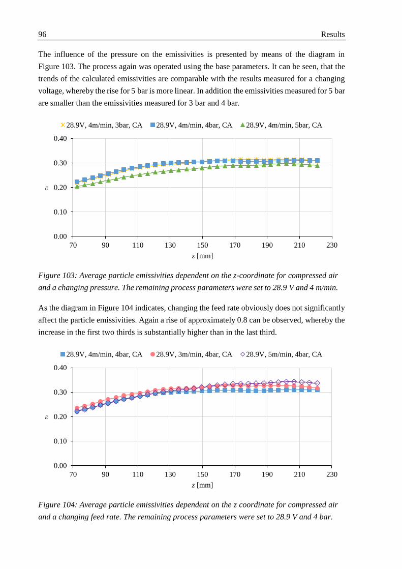
96 Results
The influence of the pressure on the emissivities is presented by means of the diagram in
Figure 103. The process again was operated using the base parameters. It can be seen, that the
trends of the calculated emissivities are comparable with the results measured for a changing
voltage, whereby the rise for 5 bar is more linear. In addition the emissivities measured for 5 bar
are smaller than the emissivities measured for 3 bar and 4 bar.
As the diagram in Figure 104 indicates, changing the feed rate obviously does not significantly
affect the particle emissivities. Again a rise of approximately 0.8 can be observed, whereby the
increase in the first two thirds is substantially higher than in the last third.
0.00
0.10
0.20
0.30
0.40
70 90 110 130 150 170 190 210 230
ε
z [mm]
28.9V, 4m/min, 3bar, CA 28.9V, 4m/min, 4bar, CA 28.9V, 4m/min, 5bar, CA
0.00
0.10
0.20
0.30
0.40
70 90 110 130 150 170 190 210 230
ε
z [mm]
28.9V, 4m/min, 4bar, CA 28.9V, 3m/min, 4bar, CA 28.9V, 5m/min, 4bar, CA
Figure 103: Average particle emissivities dependent on the z-coordinate for compressed air
and a changing pressure. The remaining process parameters were set to 28.9 V and 4 m/min.
Figure 104: Average particle emissivities dependent on the z coordinate for compressed air
and a changing feed rate. The remaining process parameters were set to 28.9 V and 4 bar.
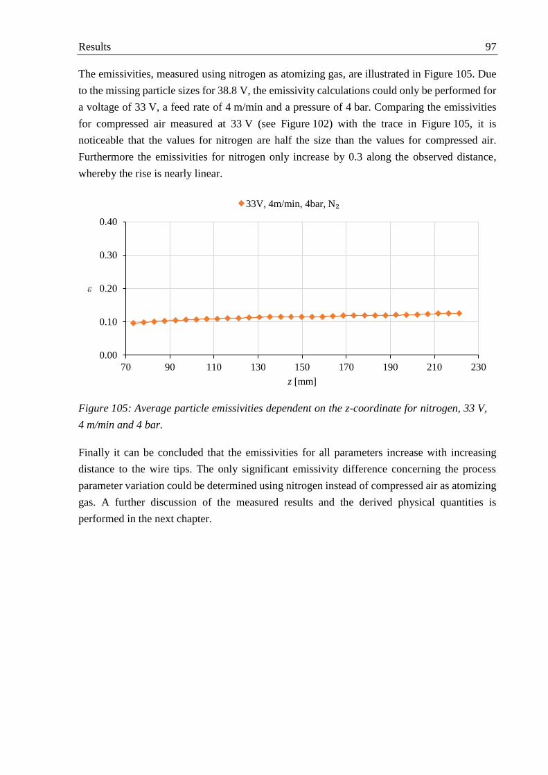
Results 97
The emissivities, measured using nitrogen as atomizing gas, are illustrated in Figure 105. Due
to the missing particle sizes for 38.8 V, the emissivity calculations could only be performed for
a voltage of 33 V, a feed rate of 4 m/min and a pressure of 4 bar. Comparing the emissivities
for compressed air measured at 33 V (see Figure 102) with the trace in Figure 105, it is
noticeable that the values for nitrogen are half the size than the values for compressed air.
Furthermore the emissivities for nitrogen only increase by 0.3 along the observed distance,
whereby the rise is nearly linear.
Finally it can be concluded that the emissivities for all parameters increase with increasing
distance to the wire tips. The only significant emissivity difference concerning the process
parameter variation could be determined using nitrogen instead of compressed air as atomizing
gas. A further discussion of the measured results and the derived physical quantities is
performed in the next chapter.
0.00
0.10
0.20
0.30
0.40
70 90 110 130 150 170 190 210 230
ε
z [mm]
33V, 4m/min, 4bar, N₂
Figure 105: Average particle emissivities dependent on the z-coordinate for nitrogen, 33 V,
4 m/min and 4 bar.

98 Discussion
7 Discussion
To be able to estimate possible error sources of the in-flight oxidation determination all single
measurement results that contribute to the model have to be verified. According to Equation 4.6
the particle sizes, the particle velocities and the particle temperatures are among other things
necessary for the calculation of the emissivity. Furthermore the tomographic
two-color-pyrometry results including the temperature and emissivity measurements are
discussed.
7.1 Particle size and velocity measurements
The particle sizes are measured by means of PSI (see Chapter 5.3 and Chapter 6.4), whereby
the measurement volume is located in the middle of the spray plume 70 mm in front of the wire
tips. Since it is difficult to find values for the particle size in literature that are measured using
the same nozzle geometry, the same feedstock and the same process parameters, the accuracy
of the PSI results can only qualitatively be evaluated. First of all the influence of the process
voltage on the particle size is discussed. As shown in Figure 66 and listed in Table 12, for
28.9 V a mean particle radius of 22 µm and for 33 V a mean particle radius of 22.8 µm was
measured, whereas for 38.8 V the radius increases to 25 µm. According to Kelkar et al. [148]
the size of droplets detached from the cathode depends on the electromagnetic pinch effect (first
term on the left hand side of Equation 7.1), the aerodynamic drag (second term), the weight
force (third term) and the surface tension (right hand side).
4
2 2 30 1 4cos
4 2 2 3
: radius of the spherical droplet
: radius of the wire
: drag coefficient
, : density of the atomizing gas and the wire, respectively
: relative
d g rel drop
d
g
rel
aI C v A a g a
b
a
b
C
v
velocity between the gas and the droplet
: cross section area of the droplet
: angle between the wires
: surface tension
dropA
7.1
Because on the anode in contrast to the cathode long non current-carrying sheets are formed,
the size of the anode particles is only influenced by the gas flow and the surface tension
(Equation 7.2).
21
2d g rel drop dropC v A l 7.2

Discussion 99
Since with increasing voltage the heat input (see Figure 59) and consequently the particle
temperatures (see Figure 98) increase, the temperature dependent surface tension that keeps
liquid material attached decreases [149]. Furthermore, the current rises with increasing voltage
leading to an increase of the electromagnetic force. To conclude, these two effects should cause
smaller particles and consequently, the increase of the particle radius from 22 µm for 28.9 V to
25 µm for 38.8 V can only be explained with changed flow conditions. How the typical high
speed images of the wire arc spray process illustrated in Figure 106 show, there are significant
detachment differences between operating the process with 28.9 V and operating the process
with 38.8 V. At 28.9 V the particle replacement is concentrated between the two tips, whereas
the replacement at 38.8 V is shifted outwards. Since the flow velocity probably decreases with
increasing distance to the spraying axis, the atomization of the detached particles decreases for
higher voltages and consequently the discrepancy between Kelkar’s model and the measured
particle sizes can be explained.
The influence of the pressure on the particle size seems to be easier to explain. Using again the
model of Kelkar et al., it is obvious that with increasing gas flow and consistent other process
parameters the particle size decreases. This trend was for example measured by Liao et al. [36]
using copper as anode wire and steel as cathode wire and vice versa in order to be able to
separate the collected anode and cathode particles with the help of a magnet. The size
distributions, determined using a particle size analyzer, show both for steel particles detached
from the anode and the steel particles detached from the cathode a decreasing particle size for
an increasing pressure. For 2.8 bar they measured a mean anode particle diameter of 52 µm and
a mean cathode particle diameter of 44 µm, for a pressure of 4.9 bar 39 µm and 28 µm The
other process parameters used by Liao (200 A, 30 V) are comparable to the base parameters. In
this work for 3 bar an average particle diameter of 44.8 µm was determined, for 4 bar a diameter
of 44 µm and for 5 bar a mean particle diameter of 40.6 µm. Consequently the trend of
decreasing particle sizes with increasing pressure could be confirmed.
In the case of a changing wire feed rate, the different influences on the particle size are more
complex to explain. On the one hand the flow keeps constant and on the other hand the amount
of material to be fused, the current and the voltage (see Appendix A.4) change with changing
Figure 106: High speed images of the wire arc spray process acquired for 28.9 V and 38.8 V.
The other parameters were set to the base parameters and compressed air was used as gas.

100 Discussion
feed rate. Based on the velocity measurements presented in Figure 73, the mean particle radius
for 4 bar should be smaller than the radii measured for 3 bar and 5 bar, whereby the values for
3 bar in turn should be between 4 bar and 5 bar. Looking at diagram d) in Figure 66 this trend
can be confirmed, although the difference between the mean particle radii measured for
3 m/min and 4 m/min might be too low.
For the usage of nitrogen as gas, a voltage of 33 V, a feed rate of 4 m/min and a pressure of
4 bar the measured mean particle radius is 22.6 µm. This value is almost equal to the radius
measured using compressed air and the same parameters (22.8 µm). Since nitrogen causes a
higher surface tension than oxygen [150] the detached particles should be larger. Another
indicator therefore are again the velocity measurements (Figure 74). For a voltage of 33 V the
velocities using nitrogen are approximately 10 m/s lower than the velocities measured using
compressed air. The too small average particle radius for nitrogen may be caused by the image
processing steps applied to the PSI images. Since it is more likely that great particles touch the
fringe of the region of interest and therefore are ignored, they are underrepresented what in turn
is more pronounced for using nitrogen as atomizing gas.
In summary, the mean particle radii for all investigated parameters are between 20.3 µm and
25.1 µm (compare Table 12). Due to this small variation and the all in all accordance of the
velocity trends and the particle sizes trends, the measured mean particle radii are suitable for
the emissivity calculations.
The measured particle velocities again can only qualitatively be evaluated, because no particle
velocity investigations using the same arc spray gun and consequently the same nozzle
configuration could be found in literature. Comparable measurements are performed by
Newbery et al. [33] using laser two-focus velocimetry (L2F). Results of their work are presented
in Figure 107. The velocities were measured in the middle of the spray plume at a voltage of
34 V, a feed rate of 1 g/s (≙ 3.8 m/min) and a pressure of 2.8 bar. As atomizing gas compressed
air was used. Since the influence of the voltage on the particle velocity is less than the influence
of the pressure, the most comparable parameters of this work are 28.9 V, 4 m/min and 3 bar
(also presented in Figure 107). The velocities measured by Newbery slightly increase from
104 m/s at 70 mm to 109 m/s at 120 mm and subsequently decrease to 103 m/s at 200 mm.
Responsible for the lower velocities may be the higher voltage and the lower pressure. The
increasing and subsequently decreasing particle velocitiy along the spraying direction is also
observed by Hale et al. [32] for spraying aluminum and Tillmann et al. [151] for spraying
massive steel wires. The simulations and the measurements of Prehm [152] show that the gas
velocity steadily declines with increasing distance to the wire tips and consequently the
detached particles are accelerated until they reach the gas velocity and are subsequently slowed
down.
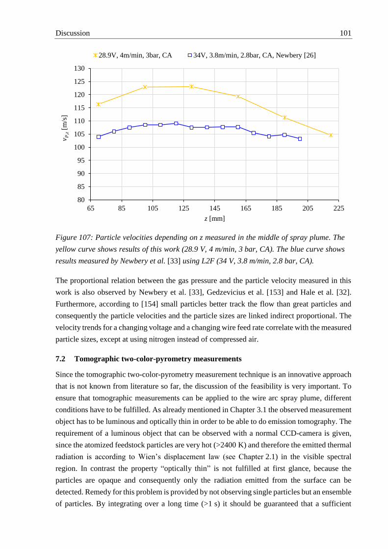
Discussion 101
The proportional relation between the gas pressure and the particle velocity measured in this
work is also observed by Newbery et al. [33], Gedzevicius et al. [153] and Hale et al. [32].
Furthermore, according to [154] small particles better track the flow than great particles and
consequently the particle velocities and the particle sizes are linked indirect proportional. The
velocity trends for a changing voltage and a changing wire feed rate correlate with the measured
particle sizes, except at using nitrogen instead of compressed air.
7.2 Tomographic two-color-pyrometry measurements
Since the tomographic two-color-pyrometry measurement technique is an innovative approach
that is not known from literature so far, the discussion of the feasibility is very important. To
ensure that tomographic measurements can be applied to the wire arc spray plume, different
conditions have to be fulfilled. As already mentioned in Chapter 3.1 the observed measurement
object has to be luminous and optically thin in order to be able to do emission tomography. The
requirement of a luminous object that can be observed with a normal CCD-camera is given,
since the atomized feedstock particles are very hot (>2400 K) and therefore the emitted thermal
radiation is according to Wien’s displacement law (see Chapter 2.1) in the visible spectral
region. In contrast the property “optically thin” is not fulfilled at first glance, because the
particles are opaque and consequently only the radiation emitted from the surface can be
detected. Remedy for this problem is provided by not observing single particles but an ensemble
of particles. By integrating over a long time (>1 s) it should be guaranteed that a sufficient
80
85
90
95
100
105
110
115
120
125
130
65 85 105 125 145 165 185 205 225
v P,z
[m/s
]
z [mm]
28.9V, 4m/min, 3bar, CA 34V, 3.8m/min, 2.8bar, CA, Newbery [26]
Figure 107: Particle velocities depending on z measured in the middle of spray plume. The
yellow curve shows results of this work (28.9 V, 4 m/min, 3 bar, CA). The blue curve shows
results measured by Newbery et al. [33] using L2F (34 V, 3.8 m/min, 2.8 bar, CA).

102 Discussion
number of particles flies through every point of the measurement volume so that the acquired
smooth 2D images reflect statistical particle distributions. The preconditions for this are a
stationary and an optically thin spray plume, whereby the property optically thin ensures that
the radiation of almost all particles receives the detector without being shaded by other particles.
The stability of the wire arc spray process can be proved by the voltage and current
measurements. As Figure 122 to Figure 129 in the Appendix A.4 show, the voltage and current
traces do not show any short circuits or other long-lasting disturbances. All current and voltage
fluctuations take place in a period of less than 5 ms and are consequently averaged over the
integration time. The optical thickness of the spray plume is determined through using the LDA,
PSI and DPV measurements as input for the model developed in Chapter 3.2. Since the
calculated optical thickness for all used parameters is below 0.05 (see Chapter 6.5), the
condition optically thin ( 1 [119, 120]) is fulfilled in any case.
Besides this theoretical considerations, the 3D reconstructions itself are evidence for an
optically thin spray plume, since they do not show any artifacts caused by too high optical
thickness. Looking for example at the computerized tomography (CT) used in medicine, an
object that is not optically thin for the X-Ray radiation is given by metal. If there is metal in the
body of a patient e.g. in the form of solid amalgam tooth fillings, so called strike artifacts can
be seen in the reconstructions [116]. An example for such an erroneous CT image is presented
on the left side of Figure 108. For comparison on the right side a reconstructed cross section of
the spray plume that does not show any artifacts is illustrated.
To conclude, the wire arc spray plume is suitable for tomographic investigations, whereby it
has to be noted that only the radiation emitted from the surface can be reconstructed and hence
only surface temperatures can be determined.
The structure of the 3D intensity reconstructions (Figure 80 to Figure 88) presented in the
previous chapter depends according to Equation 4.3 on the particle size, velocity rate,
temperature and emissivity. Because of the interdependence of all these different parameters
Figure 108: Left: CT image of the tooth region showing strike artifacts caused by solid
amalgam fillings (adopted from [116]). Right: cross section of the reconstructed spray plume
without any artifacts.
Discussion 103
the 3D reconstructions only allow qualitative conclusions. Thus for example the intensity
distributions for a changing pressure show a strong constriction of the spray plume with
increasing pressure, which in turn is confirmed by the LDA results presented in Figure 68.
Consequently, the intensity distributions for a changing pressure seem to be strongly connected
to the spatial resolved particle rates. Also in the case of a changing wire feed rate the
reconstructed intensities seem to be proportional to the particle rate, since both the rates
measured with the LDA (see Figure 69) and the intensities measured with the tomography
strongly increase with increasing feed rate. Finally it can be stated that the tomographic 3D
intensity reconstruction is a useful tool in order to visualize the expansion of the spray plume.
More interesting is the processing of the obtained intensity data. By voxel vice dividing of the
two intensity distributions measured with the two-color-pyrometry and comparing the results
with calculated quotients, spatial resolved temperature distributions can be determined (see
Chapter 3.3.2). As already mentioned, the 3D visualization of the temperature distributions is
not very informative, because the deviation of the temperatures is low and the distributions are
not very homogenous (compare Figure 89). However, the cross sections in the xy-plane are
suitable to show the general influence of the different parameters on the particle temperature.
Furthermore, the cross sections are used in order to calculate the average temperatures along
the spraying direction that in turn are necessary for the emissivity calculation.
Looking at the average temperatures determined for a changing voltage (see Figure 98), it is
obvious that increasing the voltage leads to an increasing particle temperature. The reason for
this behavior is the heat input that according to Figure 59 a) declines proportional to the rising
voltage. After the heated and molten particles are detached they are atomized and are exposed
to various influences. On the one hand they are heated due to exothermic oxidation [33, 72] and
on the other hand they are cooled down due to convection and radiation losses [32, 34]. As the
temperature traces for all three voltages decrease with increasing distance to the wire tips, the
heat loses due to convection and radiation generally seem to be higher than the heating due to
oxidation. It can be noted that the temperature drop for high initial temperatures is greater than
for low temperatures. Responsible therefore may be the higher heat transfer caused by the
higher difference temperature.
The influence of the gas pressure on the average particle temperature is according to Figure 99
not significant. Increasing the pressure from 3 bar to 5 bar causes a temperature difference of
approximately 50 K at a distance of 70 mm. The reason for this temperature difference may be
on the one hand the decreasing gas temperatures for an increasing pressure and on the other
hand the decreasing particle sizes for an increasing pressure leading to a larger effective surface
and consequently to more heat losses due to radiation an convection. The heat input for the
three investigated pressures is according to Figure 59 c) almost constant. A small temperature
drop along the spraying direction can be observed again.

104 Discussion
To explain the influence of the wire feed rate on the average particle temperature again the
calculated heat inputs per mass can be used. Figure 59 d) shows an indirect proportional relation
between the feed rate and the heat input. This connection can also be found at the measured
average temperatures (see Figure 100).
Using nitrogen instead of compressed air strongly affects the average particle temperatures.
Comparing the traces for nitrogen in Figure 101 with the traces for compressed air in Figure 98,
it can be seen that the temperatures using nitrogen are ~150 K lower for 33 V and ~80 K lower
for 38.8 V. A possible explanation therefore are, besides the lower oxidation using nitrogen [33,
72], the differences in heat input. The results presented in Figure 59 show that the heat input
for nitrogen at 33 V is approximately 10 % lower than the heat input for compressed air at 33 V
and that the input for nitrogen at 38.8 V is approximately 8 % lower than the heat input for
compressed air at 38.8 V. Responsible for the lower electric energy input are the higher
dissociation energy and ionization energy of nitrogen compared to oxygen [155] leading to a
higher electrical resistance of the arc and consequently to a lower current at the same voltage.
To be able to estimate if the measured average temperatures are in a plausible range, the results
have to be compared with data from literature. The measured particle temperatures are again
most likely comparable with the results obtained by Newbery et al. [33]. The temperature
determination in their work is performed using a two-color pyrometer that is calibrated with the
help of a tungsten ribbon standard. They measured the temperature along the spraying direction
for a voltage of 34 V, a feed rate of 3.8 m/min and pressure of 2.8 bar. Compressed air was used
as atomizing gas. Because the voltage is the most temperature influencing parameter, the
parameters used in this work that should cause the most comparable temperatures are a voltage
of 33 V, a feed rate of 4 m/min and a pressure of 4 bar. The results measured in this work and
the results measured by Newbery et al. are presented in Figure 109. The temperatures from
Newbery et al. decrease from 2638 K at 70 mm to 2539 K at 200 mm and are approximately
100 K lower than the temperatures measured in this work. Since the voltage used by Newbery
et al. is higher and the feed rate and the pressure are lower, the measured temperatures should
according to the above discussed trends actually be higher. As Newbery et al. mention,
responsible for the too low temperatures is the underestimation up to 250 K caused by the
assumption that the steel particles have the same emissivity ratio as tungsten at the two widely
separated filter wavelengths (950 nm and 1350 nm). Taking this underestimation into account
the temperatures of Newbery et al. are above the temperatures measured in this work and
therefore would better match to the discussed tendencies.
All in all it can be noted that the measured particle temperatures are in good agreement with
literature and that the determined trends fit well together with the current and voltage
measurements. Finally, the tomographic two-color-pyrometry is a suitable diagnostic allowing
average particle temperature determination along the spraying direction without the need of
scanning the whole spray plume.

Discussion 105
Besides the application of the tomographic measurement technique on the wire arc spray plume,
the in-flight determination of material depended emissivities is the innovative approach of this
work. Using the model presented in Chapter 4 and the tomographic two-color-pyrometry, the
PSI and the DPV results as input, the average particle emissivities can be calculated. Since all
emissivities measured at a wavelength of 800 nm (see Figure 102 to Figure 105) are between
0.1 and 0.35, the emissivity of liquid S235 above 2100 K (S235 0.087 compare Table 7)
measured by Schöpp et al. [132] seems to be the most suitable value for the iron based feedstock
material used in this work. Furthermore for the emissivity of liquid FeO (FeO 0.7 compare
Table 7) the value of Muller et al. [133] has to be used to discuss the results, because no other
values could be found in literature for temperatures above 2100 K.
Assuming that the unoxidized material and the dominating oxide FeO are mixed continuously
and thus the surface is measure for the degree of oxidation of the whole particle, the in-flight
oxide content depending on z can be estimated by Equation 7.3.
S235
FeO S235
100 %ox
zC z
7.3
To be able to evaluate the in-flight oxide content, it is assumed that the oxide area fractions
presented in Chapter 6.3 represent the absolute oxide content of the test coatings and that these
oxides are only caused by particle in-flight oxidation and not by the post-oxidation of the splat
surfaces. This assumption may be justified, since the wire arc spray process is a process with
high deposition rates leading to short times between the impingement of two consecutive
2500
2550
2600
2650
2700
2750
70 90 110 130 150 170 190 210 230
Ta
vg [
K]
z [mm]
33V, 4m/min, 4bar, CA 34V, 3.8m/min, 2.8bar, CA, Newbery [26]
Figure 109: Particle temperatures depending on z measured in the middle of spray plume.
The orange curve shows results of this work. The blue curve shows results measured by
Newbery et al. [33] using a two-color pyrometer.

106 Discussion
particles. Furthermore, the dwell time of the particles in the gas stream is compared to other
thermal spray process (e.g. HVOF) long [43], whereby the degree of in-flight oxidation is high.
The diagrams in Figure 110 to Figure 113 show the comparison of the test coating oxide
contents and the particle oxide contents for the different investigated parameter sets. With
compressed air as atomizing gas, the measured particle oxide contents tend to be higher than
the oxide contents determined for the test coatings. Furthermore in contrast to the coating oxide
contents, the particle oxide contents do not linearly increase, but slowly go into saturation. Both
observations are evidence that the feedstock material and the oxides do not continuously mix.
Instead, it is assumed that the oxidation on the particle surfaces initially progresses fast and
subsides with increasing oxide shell. Nevertheless, the relative increase of the particle oxide
contents along the observed distance is in good agreement with the increase of the oxide
contents of the test coatings. However, it is not possible to measure the trend of the changing
parameters. For example, the proportional relations between the pressure and the oxide content
and the feed rate and the oxide content cannot be found in the in-flight oxidation measurements.
As Figure 113 shows, the particle oxide contents calculated for nitrogen as atomizing gas are
significantly smaller than the corresponding test coating oxide contents. Responsible therefore
is most probably the too low particle size measured with the PSI (see discussion in Chapter 7.1).
Through inserting Equation 4.4 into Equation 4.6 it can be seen that the emissivity and
consequently the particle oxide content are direct proportional to the particle radius. To clarify
the influence of the particle size, the particle oxide content trace calculated for a 45 % increased
particle radius is presented in Figure 113. Apart from that, both the slope of the original particle
oxide contents and the slope of the modified particle oxide contents are in good agreement with
the slope of the coating oxide contents. Due to the significant lower degree of oxidation no
saturation can be observed.
To conclude, the tomographic two-color-pyrometry in combination with particle size and
velocity measurements offers the possibility of in-flight oxidation measurements. The results
are in good agreement with the oxide contents of sprayed coatings. To obtain more precise
results it may be necessary to perform spatial resolved particle size and velocity measurements
along the spraying direction.

Discussion 107
45 65 85 105 125 145 165 185 205 225 245
0
5
10
15
20
25
30
35
40
45
0
5
10
15
20
25
30
35
40
45
65 105 145 185 225
Oxid
e co
nte
nt
[%]
z [mm]
28.9 V, coatings 33 V, coatings 38.8 V, coatings
28.9 V, particles 33 V, particles 38.8 V, particles
45 95 145 195 245
0
5
10
15
20
25
30
35
40
45
0
5
10
15
20
25
30
35
40
45
65 105 145 185 225
Oxid
e co
nte
nt
[%]
z [mm]
3 bar, coatings 4 bar, coatings 5 bar, coatings
3 bar, particles 4 bar, particles 5 bar, particles
Figure 110: Comparison of test coating oxide contents and in-flight measured particle oxide
contents. The process was operated with CA, 4 m/min, 4 bar and three different voltages.
Figure 111: Comparison of test coating oxide contents and in-flight measured particle oxide
contents. The process was operated with CA, 28.9 V, 4 m/min and three different pressures.
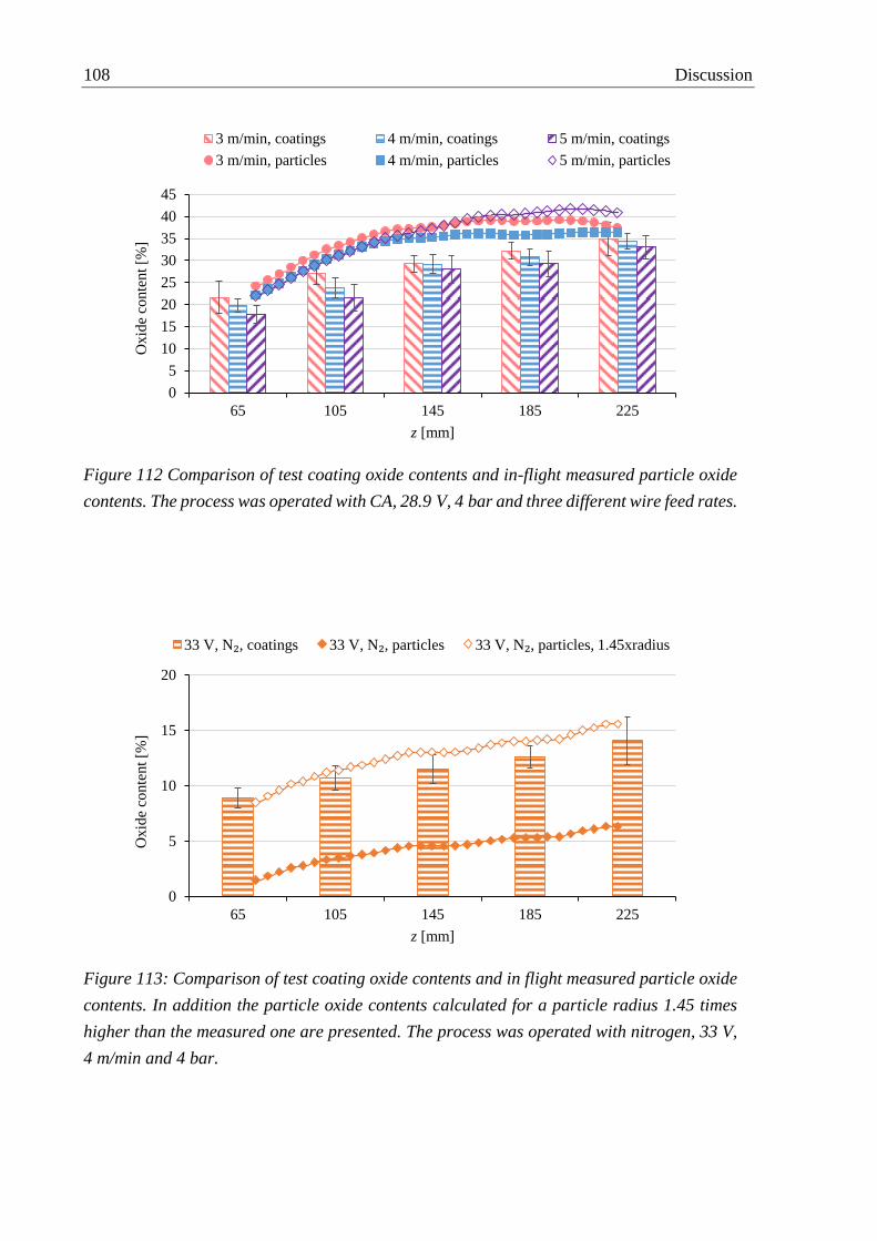
108 Discussion
45 95 145 195 245
0
5
10
15
20
25
30
35
40
45
0
5
10
15
20
25
30
35
40
45
65 105 145 185 225
Oxid
e co
nte
nt
[%]
z [mm]
3 m/min, coatings 4 m/min, coatings 5 m/min, coatings
3 m/min, particles 4 m/min, particles 5 m/min, particles
45 95 145 195 245
0
2
4
6
8
10
12
14
16
18
20
0
5
10
15
20
65 105 145 185 225
Oxid
e co
nte
nt
[%]
z [mm]
33 V, N₂, coatings 33 V, N₂, particles 33 V, N₂, particles, 1.45xradius
Figure 112 Comparison of test coating oxide contents and in-flight measured particle oxide
contents. The process was operated with CA, 28.9 V, 4 bar and three different wire feed rates.
Figure 113: Comparison of test coating oxide contents and in flight measured particle oxide
contents. In addition the particle oxide contents calculated for a particle radius 1.45 times
higher than the measured one are presented. The process was operated with nitrogen, 33 V,
4 m/min and 4 bar.
Conclusion 109
8 Conclusion
Thermal spraying is the generic term for processes that provide a high amount of energy in
order to melt and atomize feedstock material that is finally accelerate towards a substrate to be
coated. Due to the broad available power range, a great variety of feedstock materials and their
combinations can be used to improve the surface properties of the base material. Decisive for
the quality of a coating are the proper selection of materials and gases as well as a conscientious
substrate preparation. Important parameters that cannot be proved beforehand and that may
change during the coating process are the properties of the atomized particles. The velocity, the
size, the temperature and the rate influence for example the adhesion to the substrate, the
cohesion between the splats or the hardness of the coating. A key factor that is strongly
connected to the before-mentioned coating properties is the oxide content, whereby a high
amount of oxides depending on the requirements on the coating can both be desirable or
undesirable. The oxide content in turn strongly depends on the in-flight oxidation of the
particles and consequently on their temperature, size and velocity. For the measurement of these
properties many diagnostics for industry and for research purpose are available and known.
However, the determination of the particle in-flight oxidation based on these diagnostics and
their results can only be done qualitatively, since the influence of the used process gases and
the surrounding environment is not taken into account. For these reasons the approach of this
work is the development of a thermal spraying diagnostic allowing quantitative conclusions on
the in-flight particle oxidation.
The innovative diagnostic combines two-color-pyrometry with tomographic recording and
evaluation techniques. Observing the spray plume at two different wavelength bands from
different directions enables the determination of three dimensional intensity and temperature
distributions. The measured total intensity along the spraying direction depends on the particle
rate, velocity, size, temperature and emissivity. Since the emissivities for the used feedstock
material and the resulting oxides are known form literature and the temperature and the
intensities are measured using the tomographic two-color-pyrometry, it is possible to determine
the in-flight particle oxide content. Whereby the velocities and sizes have to be measured using
the established diagnostics DPV and PSI.
The two-color-pyrometry setup consist of a beam splitter and two CCD-cameras with different
interference filters in front. All components are chosen in a way that the error due the
assumption of gray body behavior and the error caused by measurement uncertainties are low.
Furthermore, for every pixel of the cameras a calibration factor is determined using a moving
tungsten calibration lamp, whose temperature is spectroscopically measured.
The two-color-pyrometry module is moved around the spray plume and acquires images in
defined angle steps with a long exposure time (>1 s). By applying the so called algebraic
reconstruction technique on the raw data three dimensional intensity distributions for the two
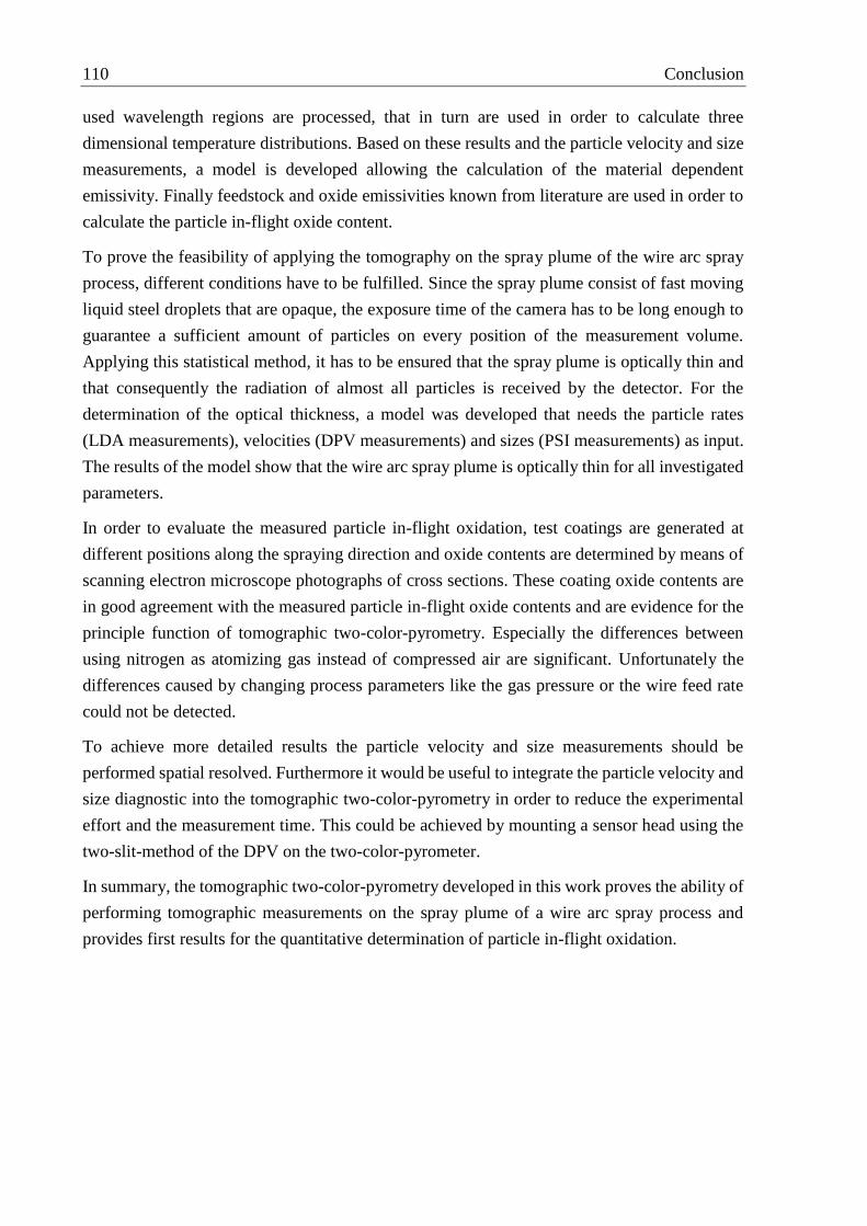
110 Conclusion
used wavelength regions are processed, that in turn are used in order to calculate three
dimensional temperature distributions. Based on these results and the particle velocity and size
measurements, a model is developed allowing the calculation of the material dependent
emissivity. Finally feedstock and oxide emissivities known from literature are used in order to
calculate the particle in-flight oxide content.
To prove the feasibility of applying the tomography on the spray plume of the wire arc spray
process, different conditions have to be fulfilled. Since the spray plume consist of fast moving
liquid steel droplets that are opaque, the exposure time of the camera has to be long enough to
guarantee a sufficient amount of particles on every position of the measurement volume.
Applying this statistical method, it has to be ensured that the spray plume is optically thin and
that consequently the radiation of almost all particles is received by the detector. For the
determination of the optical thickness, a model was developed that needs the particle rates
(LDA measurements), velocities (DPV measurements) and sizes (PSI measurements) as input.
The results of the model show that the wire arc spray plume is optically thin for all investigated
parameters.
In order to evaluate the measured particle in-flight oxidation, test coatings are generated at
different positions along the spraying direction and oxide contents are determined by means of
scanning electron microscope photographs of cross sections. These coating oxide contents are
in good agreement with the measured particle in-flight oxide contents and are evidence for the
principle function of tomographic two-color-pyrometry. Especially the differences between
using nitrogen as atomizing gas instead of compressed air are significant. Unfortunately the
differences caused by changing process parameters like the gas pressure or the wire feed rate
could not be detected.
To achieve more detailed results the particle velocity and size measurements should be
performed spatial resolved. Furthermore it would be useful to integrate the particle velocity and
size diagnostic into the tomographic two-color-pyrometry in order to reduce the experimental
effort and the measurement time. This could be achieved by mounting a sensor head using the
two-slit-method of the DPV on the two-color-pyrometer.
In summary, the tomographic two-color-pyrometry developed in this work proves the ability of
performing tomographic measurements on the spray plume of a wire arc spray process and
provides first results for the quantitative determination of particle in-flight oxidation.
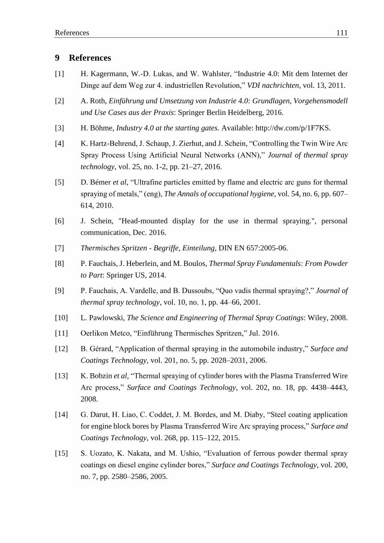
References 111
9 References
[1] H. Kagermann, W.-D. Lukas, and W. Wahlster, “Industrie 4.0: Mit dem Internet der
Dinge auf dem Weg zur 4. industriellen Revolution,” VDI nachrichten, vol. 13, 2011.
[2] A. Roth, Einführung und Umsetzung von Industrie 4.0: Grundlagen, Vorgehensmodell
und Use Cases aus der Praxis: Springer Berlin Heidelberg, 2016.
[3] H. Böhme, Industry 4.0 at the starting gates. Available: http://dw.com/p/1F7KS.
[4] K. Hartz-Behrend, J. Schaup, J. Zierhut, and J. Schein, “Controlling the Twin Wire Arc
Spray Process Using Artificial Neural Networks (ANN),” Journal of thermal spray
technology, vol. 25, no. 1-2, pp. 21–27, 2016.
[5] D. Bémer et al, “Ultrafine particles emitted by flame and electric arc guns for thermal
spraying of metals,” (eng), The Annals of occupational hygiene, vol. 54, no. 6, pp. 607–
614, 2010.
[6] J. Schein, "Head-mounted display for the use in thermal spraying.", personal
communication, Dec. 2016.
[7] Thermisches Spritzen - Begriffe, Einteilung, DIN EN 657:2005-06.
[8] P. Fauchais, J. Heberlein, and M. Boulos, Thermal Spray Fundamentals: From Powder
to Part: Springer US, 2014.
[9] P. Fauchais, A. Vardelle, and B. Dussoubs, “Quo vadis thermal spraying?,” Journal of
thermal spray technology, vol. 10, no. 1, pp. 44–66, 2001.
[10] L. Pawlowski, The Science and Engineering of Thermal Spray Coatings: Wiley, 2008.
[11] Oerlikon Metco, “Einführung Thermisches Spritzen,” Jul. 2016.
[12] B. Gérard, “Application of thermal spraying in the automobile industry,” Surface and
Coatings Technology, vol. 201, no. 5, pp. 2028–2031, 2006.
[13] K. Bobzin et al, “Thermal spraying of cylinder bores with the Plasma Transferred Wire
Arc process,” Surface and Coatings Technology, vol. 202, no. 18, pp. 4438–4443,
2008.
[14] G. Darut, H. Liao, C. Coddet, J. M. Bordes, and M. Diaby, “Steel coating application
for engine block bores by Plasma Transferred Wire Arc spraying process,” Surface and
Coatings Technology, vol. 268, pp. 115–122, 2015.
[15] S. Uozato, K. Nakata, and M. Ushio, “Evaluation of ferrous powder thermal spray
coatings on diesel engine cylinder bores,” Surface and Coatings Technology, vol. 200,
no. 7, pp. 2580–2586, 2005.
112 References
[16] ASM International, J.R. Davis & Associates, Handbook of thermal spray technology.
Materials Park, OH: ASM International, 2004.
[17] J. Ružbarský and A. Panda, Plasma and Thermal Spraying: Springer International
Publishing, 2016.
[18] H. Assadi, F. Gärtner, T. Stoltenhoff, and H. Kreye, “Bonding mechanism in cold gas
spraying,” Acta Materialia, vol. 51, no. 15, pp. 4379–4394, 2003.
[19] T. Stoltenhoff, H. Kreye, and H. J. Richter, “An analysis of the cold spray process and
its coatings,” Journal of thermal spray technology, vol. 11, no. 4, pp. 542–550, 2002.
[20] S. Siegmann and C. Abert, “100 years of thermal spray: About the inventor Max Ulrich
Schoop,” Proceedings of the fifth workshop RIPT (Les Rencontres Internationales sur
la Projection Thermique), vol. 220, pp. 3–13, 2013.
[21] Oerlikon Metco, “Hochgeschwindigkeits-Flammspritzen (HVOF),”
[22] B. Irving, R. Knight, and R. W. Smith, “The HVOF process-The hottest topic in the
thermal spray industry,” Welding Journal, vol. 72, pp. 25–30, 1993.
[23] J. L Marqués, G. Forster, and J. Schein, “Multi-electrode plasma torches: motivation
for development and current state-of-the-art,” The Open Plasma Physics Journal, vol.
2, no. 1, 2009.
[24] J. Schein, J. Zierhut, M. Dzulko, G. Forster, and K. D. Landes, “Improved Plasma
Spray Torch Stability Through Multi‐Electrode Design,” Contributions to Plasma
Physics, vol. 47, no. 7, pp. 498–504, 2007.
[25] K. D. Landes, "Plasma spray apparatus for spraying powdery or gaseous material"
US5225652 A, 1993
[26] P. Haslbeck, “Entwicklung eines Dreikathoden-Plasmaspritzbrenners unter
Anwendung adaptierter plasmadiagnostischer Methoden,” Ph.D. Thesis, Universität
der Bundeswehr München, Neubiberg, 1995.
[27] M. Dzulko, “Entwicklung des Mehranoden DC-Plasmagenerators „Delta Gun“,” Ph.D.
Thesis, Universität der Bundeswehr München, Neubiberg, 2007.
[28] T. Schläfer, A. Wank, C. Schmengler, and K. Müller-Roden, “PENTA: A novel high
spray rate APS gun,” in Thermal Spray: Proceedings of the International Thermal
Spray Conference, 2017.
[29] H.-D. Steffens, Z. Babiak, and M. Wewel, “Recent developments in arc spraying,”
IEEE Transactions on Plasma Science, vol. 18, no. 6, pp. 974–979, 1990.
[30] N. A. Hussary and J. V. Heberlein, “Atomization and particle-jet interactions in the
wire-arc spraying process,” Journal of thermal spray technology, vol. 10, no. 4, pp.
604–610, 2001.

References 113
[31] N. A. Hussary and J. V. Heberlein, “Effect of system parameters on metal breakup and
particle formation in the wire arc spray process,” Journal of thermal spray technology,
vol. 16, no. 1, pp. 140–152, 2007.
[32] D. L. Hale, W. D. Swank, and D. C. Haggard, “In-flight particle measurements of twin
wire electric arc sprayed aluminum,” Journal of thermal spray technology, vol. 7, no.
1, pp. 58–63, 1998.
[33] A. P. Newbery, P. S. Grant, and R. A. Neiser, “The velocity and temperature of steel
droplets during electric arc spraying,” Surface and Coatings Technology, vol. 195, no.
1, pp. 91–101, 2005.
[34] A. Pourmousa, J. Mostaghimi, A. Abedini, and S. Chandra, “Particle size distribution
in a wire-arc spraying system,” Journal of thermal spray technology, vol. 14, no. 4, pp.
502–510, 2005.
[35] T. Watanabe, T. Sato, and A. Nezu, “Electrode phenomena investigation of wire arc
spraying for preparation of Ti-Al intermetallic compounds,” Thin Solid Films, vol. 407,
no. 1, pp. 98–103, 2002.
[36] H. L. Liao, Y. L. Zhu, R. Bolot, C. Coddet, and S. N. Ma, “Size distribution of particles
from individual wires and the effects of nozzle geometry in twin wire arc spraying,”
Surface and Coatings Technology, vol. 200, no. 7, pp. 2123–2130, 2005.
[37] A. Atzberger et al, “Thermische Plasmen: Einfluss der Strommodulation und der
verwendeten Prozessgase auf den Lichtbogendrahtspritzprozess,” Thermal Spray
Bulletin, vol. 68, no. 2, pp. 114–121, 2016.
[38] P. Fauchais, “Understanding plasma spraying,” Journal of Physics D: Applied Physics,
vol. 37, no. 9, pp. R86, 2004.
[39] J. Kotz, P. Treichel, and J. Townsend, Chemistry and Chemical Reactivity: Cengage
Learning, 2008.
[40] C. Law, Combustion Physics: Cambridge University Press, 2010.
[41] D. B. Wilson, T. A. Steinberg, and J. M. Stoltzfus, “Thermodynamics and kinetics of
burning iron,” in Flammability and Sensitivity of Materials in Oxygen-Enriched
Atmospheres: Eighth Volume: ASTM International, 1997.
[42] D. Young, High Temperature Oxidation and Corrosion of Metals: Elsevier Science,
2016.
[43] S. Deshpande, S. Sampath, and H. Zhang, “Mechanisms of oxidation and its role in
microstructural evolution of metallic thermal spray coatings—Case study for Ni–Al,”
Surface and Coatings Technology, vol. 200, no. 18–19, pp. 5395–5406, 2006.

114 References
[44] G. Espie et al, “In-flight oxidation of iron particles sprayed using gas and water
stabilized plasma torch,” Surface and Coatings Technology, vol. 195, no. 1, pp. 17–28,
2005.
[45] V. V. Sobolev and J. M. Guilemany, “Effect of oxidation on droplet flattening and
splat-substrate interaction in thermal spraying,” Journal of thermal spray technology,
vol. 8, no. 4, pp. 523–530, 1999.
[46] S. Sampath and X. Jiang, “Splat formation and microstructure development during
plasma spraying: deposition temperature effects,” Materials Science and Engineering:
A, vol. 304, pp. 144–150, 2001.
[47] C.-J. Li and W.-Y. Li, “Effect of sprayed powder particle size on the oxidation behavior
of MCrAlY materials during high velocity oxygen-fuel deposition,” Surface and
Coatings Technology, vol. 162, no. 1, pp. 31–41, 2003.
[48] M.-M. Matz and M. Aumiller, “Practical Comparison of Cylindrical Nozzle and De
Laval Nozzle for Wire Arc Spraying,” J Therm Spray Tech, vol. 23, no. 8, pp. 1470–
1477, 2014.
[49] E. Hämäläinen et al, “Imaging Diagnostics in Thermal Spraying-SprayWatch System,”
in Thermal spray surface engineering via applied research: Proceedings of the 1st
International Thermal Spray Conference, 8-11 May, 2000, Montréal, Québec, Canada,
Materials Park, OH: ASM International, 2000.
[50] F. Raletz, G. Ezo’o, M. Vardelle, and M. Ducos, “Characterization of cold-sprayed
nickel-base coatings,” in Thermal spray: Advances in technology and application:
proceedings of the International Thermal Spray Conference, Materials Park, OH: ASM
International, 2004.
[51] S. Yoon, C. Lee, H. Choi, and H. Jo, “Kinetic spraying deposition behavior of bulk
amorphous NiTiZrSiSn feedstock,” Materials Science and Engineering: A, vol. 415,
no. 1–2, pp. 45–52, 2006.
[52] J. Vattulainen, E. Hämäläinen, R. Hernberg, P. Vuoristo, and T. Mäntylä, “Novel
method for in-flight particle temperature and velocity measurements in plasma
spraying using a single CCD camera,” Journal of thermal spray technology, vol. 10,
no. 1, pp. 94–104, 2001.
[53] S. Kirner, G. Forster, and J. Schein, “Tomographic Particle Localization and Velocity
Measurement,” Journal of thermal spray technology, 2014.
[54] M. Krauss, D. Bergmann, U. Fritsching, and K. Bauckhage, “In-situ particle
temperature, velocity and size measurements in the spray forming process,” Materials
Science and Engineering: A, vol. 326, no. 1, pp. 154–164, 2002.

References 115
[55] G. Mauer, R. Vaßen, and D. Stöver, “Comparison and Applications of DPV-2000 and
Accuraspray-g3 Diagnostic Systems,” J Therm Spray Tech, vol. 16, no. 3, pp. 414–
424, 2007.
[56] C. Moreau, J.-F. Bisson, R. S. Lima, and B. R. Marple, “Diagnostics for advanced
materials processing by plasma spraying,” Pure and Applied Chemistry, vol. 77, no. 2,
pp. 443–462, 2005.
[57] Tecnar Automation Ltd, “DPV EVOLUTION: Product Manual, Edition 1,” 2012.
[58] J. Zierhut, “Entwicklung von Diagnostikverfahren zur Optimierung von
Plasmaspritzsystemen,” Ph.D. Thesis, Institut für Plasmatechnik und Mathematik,
Universität der Bundeswehr München, Neubiberg, 2000.
[59] J. Zierhut, K. D. Landes, W. Krommer, and P. Heinrich, “Particle Flux Imaging(PFI)
in-situ diagnostics for thermal coating process,” in Thermal Spray: Surface
Engineering via Applied Research : Proceedings of the 1st International Thermal
Spray Conference, Materials Park, OH: ASM International, 2000, pp. 63–66.
[60] F.-W. Bach et al, “Particle image velocimetry in thermal spraying,” 2nd International
Conference on Spray Deposition and Melt Atomization and the 5th International
Conference on Spray Forming, vol. 383, no. 1, pp. 146–152, 2004.
[61] G. E. Elsinga, B. Wieneke, F. Scarano, and A. Schröder, “Tomographic 3D-PIV and
applications,” in Particle image velocimetry: Springer, 2007, pp. 103–125.
[62] C. Baukal, Industrial Combustion Testing: CRC Press, 2010.
[63] C. Tropea, A. Yarin, and J. Foss, Springer Handbook of Experimental Fluid
Mechanics: Springer, 2007.
[64] G. Mauer et al, “Investigation and Comparison of In-Flight Particle Velocity During
the Plasma-Spray Process as Measured by Laser Doppler Anemometry and DPV-
2000,” J Therm Spray Tech, vol. 22, no. 6, pp. 892–900, 2013.
[65] W. Mayr, “Bestimmung der lokalen Geschwindigkeits- und Grössenverteilungen von
Partikeln im Plasmastrahl mittels Laser-Doppler-Anemometrie,” Ph.D. Thesis,
Fachbereich Elektrotechnik, Hochschule der Bundeswehr München, Neubiberg, 1983.
[66] A. Reusch, “Die Entwicklung eines Laser-Doppler-Meßsystems und seine Anwendung
bei Verfahren des thermischen Beschichtens,” Ph.D. Thesis, Institut für Plasmatechnik
und Mathematik, Universität der Bundeswehr München, Neubiberg, 1995.
[67] P. Lehmann, In-process Laser-Messmethoden auf der Grundlage der Fourieranalyse:
expert-Verlag, 2003.

116 References
[68] T. Streibl, “Entwicklung eines bildgebenden Partikeldiagnostikverfahrens zur
Untersuchung Thermischer Spritzprozesse,” Ph.D. Thesis, Institut für Plasmatechnik
und Mathematik, Universität der Bundeswehr München, Neubiberg, 2002.
[69] S. Zimmermann, “Particle Shape Imaging (PSI) – eine innovative Methode der
Partikeldiagnostik bei thermischen Beschichtungsverfahren,” Ph.D. Thesis, Institut für
Plasmatechnik und Mathematik, Universität der Bundeswehr München, Neubiberg,
2007.
[70] T. Streibl, K. D. Landes, and G. Forster, “PSI: new diagnostics for the determination
of particle size and shape in thermal spray processes,” in Thermal Spray: Surface
Engineering via Applied Research : Proceedings of the 1st International Thermal
Spray Conference, Materials Park, OH: ASM International, 2000, pp. 67–70.
[71] J. R. Fincke, W. D. Swank, and C. L. Jeffery, “Simultaneous Measurement of Particle
Size, Velocity, and Temperature in Thermal Plasmas,” Plasma Science, IEEE
Transactions on, vol. 18, no. 6, pp. 948–957, 1990.
[72] A. P. Newbery and P. S. Grant, “Oxidation during electric arc spray forming of steel,”
Journal of materials processing technology, vol. 178, no. 1, pp. 259–269, 2006.
[73] R. A. Neiser, M. F. Smith, and R. C. Dykhuizen, “Oxidation in wire HVOF-sprayed
steel,” Journal of thermal spray technology, vol. 7, no. 4, pp. 537–545, 1998.
[74] K. Voleník, V. Novák, J. Dubský, P. Chráska, and K. Neufuss, “Properties of alloy
steel coatings oxidized during plasma spraying,” Materials Science and Engineering:
A, vol. 234–236, pp. 493–496, 1997.
[75] J. Hlína and J. Šonský, “Time-resolved tomographic measurements of temperatures in
a thermal plasma jet,” Journal of Physics D: Applied Physics, vol. 43, no. 5, p. 55202,
2010.
[76] K. D. Landes, G. Forste, J. Zierhut, M. Dzulko, and D. Hawley, “Computer tomography
of plasma jets–applied on a TRIPLEX II torch,” in Thermal spray: Advances in
technology and application: proceedings of the International Thermal Spray
Conference, Materials Park, OH: ASM International, 2004.
[77] G. Kirchhoff, “Ueber das Verhältniss zwischen dem Emissionsvermögen und dem
Absorptionsvermögen der Körper für Wärme und Licht,” Ann. Phys. Chem, vol. 185,
no. 2, pp. 275–301, 1860.
[78] J. Stefan, Über die Beziehung zwischen der Wärmestrahlung und der Temperatur.
Wien, vol. 79.
[79] L. Boltzmann, “Ableitung des Stefan'schen Gesetzes, betreffend die Abhängigkeit der
Wärmestrahlung von der Temperatur aus der electromagnetischen Lichttheorie,” Ann.
Phys, vol. 258, no. 6, pp. 291–294, 1884.
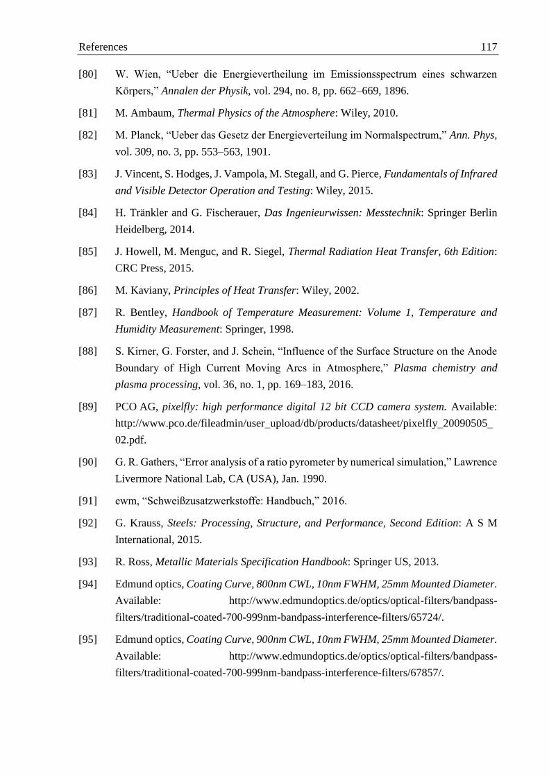
References 117
[80] W. Wien, “Ueber die Energievertheilung im Emissionsspectrum eines schwarzen
Körpers,” Annalen der Physik, vol. 294, no. 8, pp. 662–669, 1896.
[81] M. Ambaum, Thermal Physics of the Atmosphere: Wiley, 2010.
[82] M. Planck, “Ueber das Gesetz der Energieverteilung im Normalspectrum,” Ann. Phys,
vol. 309, no. 3, pp. 553–563, 1901.
[83] J. Vincent, S. Hodges, J. Vampola, M. Stegall, and G. Pierce, Fundamentals of Infrared
and Visible Detector Operation and Testing: Wiley, 2015.
[84] H. Tränkler and G. Fischerauer, Das Ingenieurwissen: Messtechnik: Springer Berlin
Heidelberg, 2014.
[85] J. Howell, M. Menguc, and R. Siegel, Thermal Radiation Heat Transfer, 6th Edition:
CRC Press, 2015.
[86] M. Kaviany, Principles of Heat Transfer: Wiley, 2002.
[87] R. Bentley, Handbook of Temperature Measurement: Volume 1, Temperature and
Humidity Measurement: Springer, 1998.
[88] S. Kirner, G. Forster, and J. Schein, “Influence of the Surface Structure on the Anode
Boundary of High Current Moving Arcs in Atmosphere,” Plasma chemistry and
plasma processing, vol. 36, no. 1, pp. 169–183, 2016.
[89] PCO AG, pixelfly: high performance digital 12 bit CCD camera system. Available:
http://www.pco.de/fileadmin/user_upload/db/products/datasheet/pixelfly_20090505_
02.pdf.
[90] G. R. Gathers, “Error analysis of a ratio pyrometer by numerical simulation,” Lawrence
Livermore National Lab, CA (USA), Jan. 1990.
[91] ewm, “Schweißzusatzwerkstoffe: Handbuch,” 2016.
[92] G. Krauss, Steels: Processing, Structure, and Performance, Second Edition: A S M
International, 2015.
[93] R. Ross, Metallic Materials Specification Handbook: Springer US, 2013.
[94] Edmund optics, Coating Curve, 800nm CWL, 10nm FWHM, 25mm Mounted Diameter.
Available: http://www.edmundoptics.de/optics/optical-filters/bandpass-
filters/traditional-coated-700-999nm-bandpass-interference-filters/65724/.
[95] Edmund optics, Coating Curve, 900nm CWL, 10nm FWHM, 25mm Mounted Diameter.
Available: http://www.edmundoptics.de/optics/optical-filters/bandpass-
filters/traditional-coated-700-999nm-bandpass-interference-filters/67857/.

118 References
[96] J. Thevenet, M. Siroux, and B. Desmet, “Measurements of brake disc surface
temperature and emissivity by two-color pyrometry,” Applied Thermal Engineering,
vol. 30, no. 6, pp. 753–759, 2010.
[97] E. C. Pyatt, “Some consideration of the errors of brightness and two-colour types of
spectral radiation pyrometer,” British Journal of Applied Physics, vol. 5, no. 7, p. 264,
1954.
[98] H. Watanabe, M. Susa, H. Fukuyama, and K. Nagata, “Phase (liquid/solid) dependence
of the normal spectral emissivity for iron, cobalt, and nickel at melting points,”
International journal of thermophysics, vol. 24, no. 2, pp. 473–488, 2003.
[99] H. Friedrich and F. Pietschmann, Numerische Methoden: ein Lehr- und Übungsbuch:
De Gruyter, 2010.
[100] T. Peifer and P. Profos, Handbuch der industriellen Messtechnik: Oldenbourg
Industrieverlag, 2008.
[101] Qioptiq Photonics GmbH u. Co. KG, Dünne Schichten – Datenblatt: ARB 2 NIR –
Breitband-Antireflex-Coating. Available: https://www.qioptiq-
shop.com/out/Graphics/en/00109153_0.pdf.
[102] S. Battiato, A. Bruna, G. Messina, and G. Puglisi, Image Processing for Embedded
Devices: Bentham Science Publishers, 2010.
[103] K. Kraus, Photogrammetry: Geometry from Images and Laser Scans: Bod Third Party
Titles, 2007.
[104] M. Katz, Introduction to Geometrical Optics: World Scientific, 2002.
[105] J. Watson and O. Zielinski, Subsea Optics and Imaging: Elsevier Science, 2013.
[106] L. Stroebel, View Camera Technique: Taylor & Francis, 1999.
[107] G. Meurant, Physical Optics and Light Measurements: Elsevier Science, 1989.
[108] Qioptiq Photonics GmbH u. Co. KG, LINOS Produkte: News & Highlights 2011.
Available: http://www.qioptiq.com/company-brochures.html.
[109] T. Vialar, Handbook of mathematics: Books on Demand, 2015.
[110] V. D. Dmitriev and G. K. Kholopov, “Spectral emissivity of a tungsten strip in the
visible and near infrared,” J Appl Spectrosc, vol. 6, no. 4, pp. 283–286, 1967.
[111] R. D. Larrabee, “The spectral emissivity and optical properties of tungsten,” Technical
report 328, Research Laboratory of Electronics, Massachusetts Institute of Technology,
Massachusetts, 1957.

References 119
[112] M. I. A. Lourakis, “A brief description of the Levenberg-Marquardt algorithm
implemented by levmar,” Institute of Computer Science, Foundation for Research and
Technology - Hellas (FORTH), Heraklion, Crete, GREECE, 2005.
[113] J. Li, Optical Delay Interferometers and Their Application for Self-coherent Detection:
KIT Scientific Publishing, 2013.
[114] M. Burke, Image Acquisition: Handbook of machine vision engineering: Springer
Netherlands, 2012.
[115] T. Matsuyama, S. Nobuhara, T. Takai, and T. Tung, 3D Video and Its Applications:
Springer London, 2012.
[116] T. M. Buzug, Computed tomography: From photon statistics to modern cone-beam CT.
Berlin: Springer, 2008.
[117] A. Ramm and A. Katsevich, The Radon Transform and Local Tomography: Taylor &
Francis, 1996.
[118] J. Radon, “Über die Bestimmung von Funktionen durch ihre Integralwerte längs
gewisser Mannigfaltigkeiten,” Berichte über die Verhandlungen der Königlich
Sächsischen Gesellschaft der Wissenschaften zu Leipzig. Mathematisch-Physische
Klasse, no. 69, pp. 262–277, 1917.
[119] A. Fridman, Plasma Chemistry: Cambridge University Press, 2008.
[120] A. Fridman and L. Kennedy, Plasma Physics and Engineering: Taylor & Francis, 2004.
[121] A. Bappert, “Tomographische Bildverarbeitung zur lokalen Bestimmung der
Emissionskoeffizienten von Plasmastrahlen,” Diplomarbeit, Institut für Grundgebiete
der Elektrotechnik, Universität der Bundeswehr München, Neubiberg, 1995.
[122] S. Kaczmarz, “Angenäherte auflösung von systemen linearer gleichungen,” Bulletin
International de l’Academie Polonaise des Sciences et des Lettres, vol. 35, pp. 355–
357, 1937.
[123] G. T. Herman, Image reconstruction from projections: The fundamentals of
computerized tomography. San Francisco: Academic Press, 1980.
[124] H. Karttunen, P. Kröger, H. Oja, M. Poutanen, and K. Donner, Fundamental
Astronomy: Springer Berlin Heidelberg, 2007.
[125] Digital Image Processing: Tata McGraw Hill Education, 2011.
[126] S. Kirner, “Bestimmung lokaler Gleichgewichts-Temperaturen thermischer Plasmen
mittels tomografischer Emissionsspektroskopie,” Diplomarbeit, Lehrstuhl für
Messsystem- und Sensortechnik, Technische Universität München, München, 2010.

120 References
[127] J. Fincke, D. Haggard, and W. Swank, “Particle temperature measurement in the
thermal spray process,” Journal of thermal spray technology, vol. 10, no. 2, pp. 255–
266, 2001.
[128] N. Birks, G. Meier, and F. Pettit, Introduction to the High Temperature Oxidation of
Metals: Cambridge University Press, 2006.
[129] D. J. Young, High temperature oxidation and corrosion of metals: Elsevier, 2008.
[130] A. Khanna, Introduction to High Temperature Oxidation and Corrosion: ASM
International, 2002.
[131] A. Ivarson, J. Powell, J. Kamalu, and C. Magnusson, “The oxidation dynamics of laser
cutting of mild steel and the generation of striations on the cut edge,” Journal of
materials processing technology, vol. 40, no. 3-4, pp. 359–374, 1994.
[132] H. Schöpp et al, “Temperature and emissivity determination of liquid steel S235,”
Journal of Physics D: Applied Physics, vol. 45, no. 23, p. 235203, 2012.
[133] M. Muller, R. Fabbro, H. El-Rabii, and K. Hirano, “Temperature measurement of laser
heated metals in highly oxidizing environment using 2D single-band and spectral
pyrometry,” Journal of laser applications, vol. 24, no. 2, p. 22006, 2012.
[134] H. Kobatake, H. Khosroabadi, and H. Fukuyama, “Normal spectral emissivity
measurement of liquid iron and nickel using electromagnetic levitation in direct current
magnetic field,” Metallurgical and Materials Transactions A, vol. 43, no. 7, pp. 2466–
2472, 2012.
[135] T. Burakowski and T. Wierzchon, Surface Engineering of Metals: Principles,
Equipment, Technologies: CRC Press, 1998.
[136] Salzgitter Flachstahl, “S235JR,” 2010.
[137] S. Ozcelik, K. Moore, and D. Naidu, Modeling, Sensing and Control of Gas Metal Arc
Welding: Elsevier Science, 2003.
[138] J. Hu and H.-L. Tsai, “Heat and mass transfer in gas metal arc welding. Part I: The arc,”
International journal of heat and mass transfer, vol. 50, no. 5, pp. 833–846, 2007.
[139] Lasertechnik Berlin, “Manual ARYELLE - Spectrograph Series,” 2009.
[140] R. Neuhauser, Anwendungen der laserinduzierten Plasmaspektroskopie (LIPS) in der
industriellen Überwachung von Schwermetall-Aerosolemissionen: Utz, Wiss, 1999.
[141] E. Loewen and E. Popov, Diffraction Gratings and Applications: Taylor & Francis,
1997.
[142] S. Zimmermann and K. Landes, “A particle image shape imaging (PSI) investigation
of particles in a plasma jet,” 2nd International Conference on Spray Deposition and
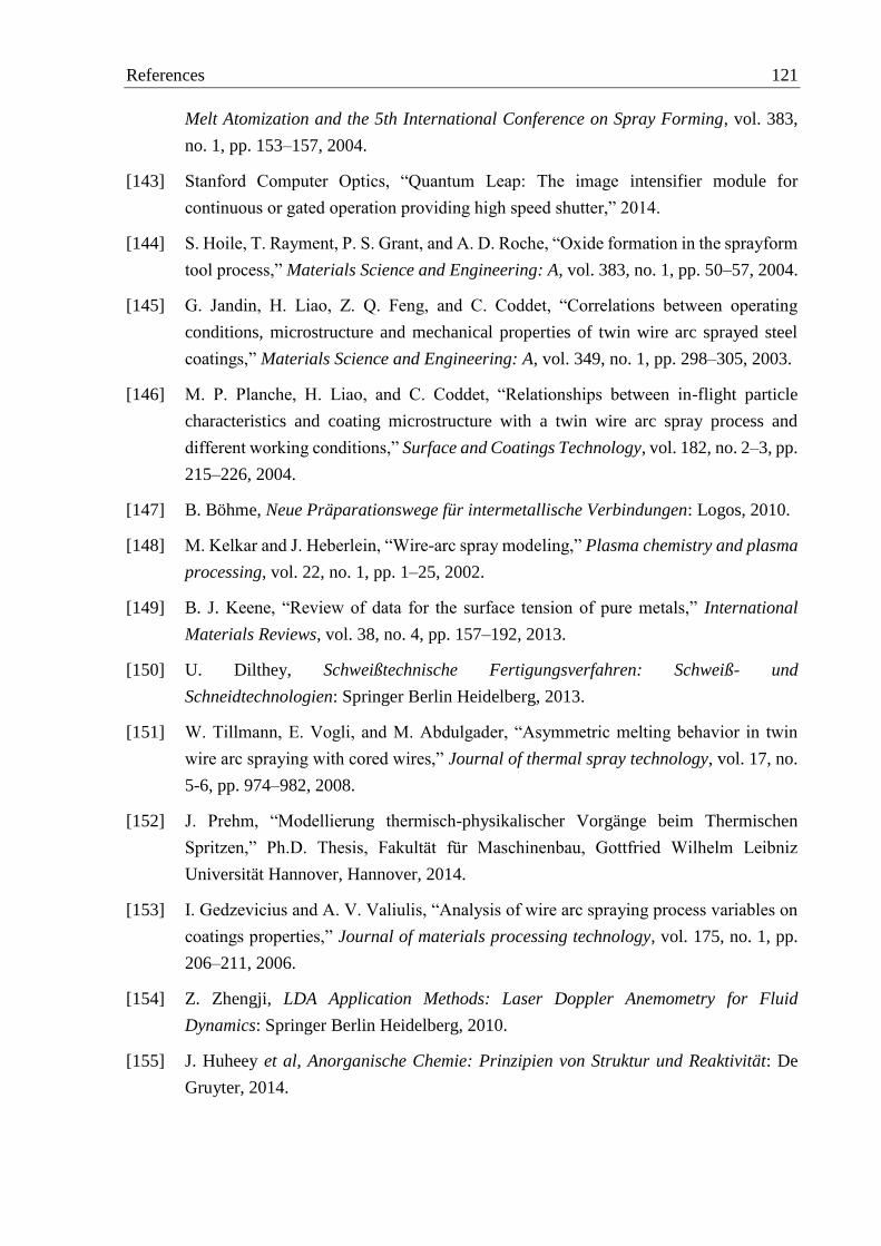
References 121
Melt Atomization and the 5th International Conference on Spray Forming, vol. 383,
no. 1, pp. 153–157, 2004.
[143] Stanford Computer Optics, “Quantum Leap: The image intensifier module for
continuous or gated operation providing high speed shutter,” 2014.
[144] S. Hoile, T. Rayment, P. S. Grant, and A. D. Roche, “Oxide formation in the sprayform
tool process,” Materials Science and Engineering: A, vol. 383, no. 1, pp. 50–57, 2004.
[145] G. Jandin, H. Liao, Z. Q. Feng, and C. Coddet, “Correlations between operating
conditions, microstructure and mechanical properties of twin wire arc sprayed steel
coatings,” Materials Science and Engineering: A, vol. 349, no. 1, pp. 298–305, 2003.
[146] M. P. Planche, H. Liao, and C. Coddet, “Relationships between in-flight particle
characteristics and coating microstructure with a twin wire arc spray process and
different working conditions,” Surface and Coatings Technology, vol. 182, no. 2–3, pp.
215–226, 2004.
[147] B. Böhme, Neue Präparationswege für intermetallische Verbindungen: Logos, 2010.
[148] M. Kelkar and J. Heberlein, “Wire-arc spray modeling,” Plasma chemistry and plasma
processing, vol. 22, no. 1, pp. 1–25, 2002.
[149] B. J. Keene, “Review of data for the surface tension of pure metals,” International
Materials Reviews, vol. 38, no. 4, pp. 157–192, 2013.
[150] U. Dilthey, Schweißtechnische Fertigungsverfahren: Schweiß- und
Schneidtechnologien: Springer Berlin Heidelberg, 2013.
[151] W. Tillmann, E. Vogli, and M. Abdulgader, “Asymmetric melting behavior in twin
wire arc spraying with cored wires,” Journal of thermal spray technology, vol. 17, no.
5-6, pp. 974–982, 2008.
[152] J. Prehm, “Modellierung thermisch-physikalischer Vorgänge beim Thermischen
Spritzen,” Ph.D. Thesis, Fakultät für Maschinenbau, Gottfried Wilhelm Leibniz
Universität Hannover, Hannover, 2014.
[153] I. Gedzevicius and A. V. Valiulis, “Analysis of wire arc spraying process variables on
coatings properties,” Journal of materials processing technology, vol. 175, no. 1, pp.
206–211, 2006.
[154] Z. Zhengji, LDA Application Methods: Laser Doppler Anemometry for Fluid
Dynamics: Springer Berlin Heidelberg, 2010.
[155] J. Huheey et al, Anorganische Chemie: Prinzipien von Struktur und Reaktivität: De
Gruyter, 2014.

122 Appendix
A Appendix
A.1 Two-color-pyrometry
Derivation of the measurement error GBE (Equation A.2) caused by the gray body assumption.
For the calculation of the temperature the Wien approximation is used (Equation A.1).
2
2
5,1 2 1
5
,2 1 2
1 1
1
ln s
s
C
TM
M
A.1
1 15 5
,1 ,12 1 12 2
2 1 ,2 2 2 ,2 2
15
,1 12
2 ,2 2
2
2
1 1 1 1ln ln
1 1
1 1ln
1
1 1
1
real measuredGB
measured
s s
s s
s
s
T TE
T
M MC C
M M
MC
M
C
1 15 5
,1 ,12 1 12
1 ,2 2 2 1 ,2 2
15
,1 12
2 ,2 2
22 2
2 2 1
1 1ln ln ln
1 1ln
1
1 1 1 1ln
1 1
s s
s s
s
s
M MC
M M
MC
M
C C
15
,1 12
,2 2 2
15 5
,1 ,12 1 12
2 1 ,2 2 ,2 2
1
2
2
1 2
1 1ln
1
1 1ln ln
1
,ln
,
1 1
s
s
s s
s s
real
real
real
MC
M
M MC
M M
TT
T
C
A.2

Appendix 123
Derivation of the temperature uncertainty (Equation A.4) caused by measurement errors. Again
for the calculation of the temperature the Wien approximation is used (Equation A.3), whereby
the spectral radiant exitance is replaced by the measured intensities 1I and
2I .
2
2 1
5
1 1
5
2 2
1 1
ln
C
TI
I
A.3
1 2
1 2
5 5 5 5
2 2 1 2 2 12 2 15 5 5 2 5
2 1 1 1 2 2 2 1 1 1 2 2
1 22 25 5
1 1 1 1
5 5
2 2 2 2
1
5
1 1
5
2 2
1 1 1 1 1 1
ln ln
1
ln
T TT I I
I I
I IC C I
I I I II I
I I
I I
TI
I
I
2
2 121 25
1 125
2 2 2 1
1 2 1 1 2 2
2 2 1 1 2 1 2 2
1 11
1 1ln
CTI
I II
CI
T T I T I
T C I C I
A.4
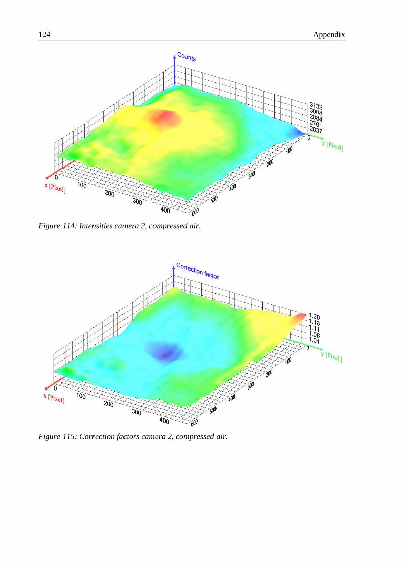
124 Appendix
Figure 114: Intensities camera 2, compressed air.
Figure 115: Correction factors camera 2, compressed air.
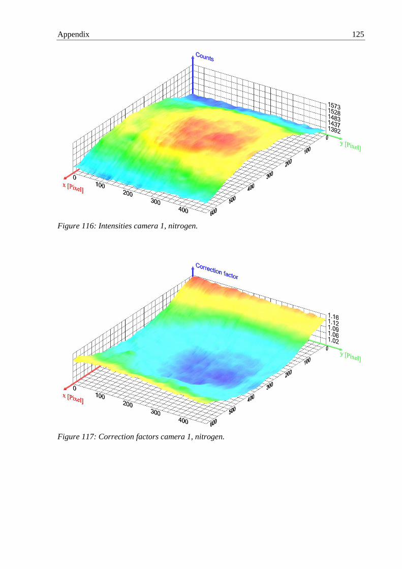
Appendix 125
Figure 116: Intensities camera 1, nitrogen.
Figure 117: Correction factors camera 1, nitrogen.

126 Appendix
Figure 118: Intensities camera 2, nitrogen.
Figure 119: Correction factors camera 2, nitrogen.

Appendix 127
A.2 Tomographic measurement of the temperature distribution
Figure 120: Program flow chart for the determination of the total intensity totI sent to the
detector and the absorbed intensity absI .

128 Appendix
A.3 General experimental settings and pretests
Equations (A.5 and A.6) for the calculation of the PSI scale using group number 5, element 1
of the 1951 USAF resolution target (see Figure 121).
32 Line pairs
Group number 5, element 1: mm
A.5
2.5 Line pairs 1000 µm µm
1.8632 Line pairs 42 Pixel Pixel
S A.6
Figure 121: Image of the 1951 USAF resolution target acquired by the PSI-diagnostic.

Appendix 129
A.4 Results
0
50
100
150
200
250
0
10
20
30
40
50
60
70
80
0 0.5 1 1.5 2
i[A
]
u[V
]
t [s]
Voltage Current
0
50
100
150
200
250
0
10
20
30
40
50
60
70
80
0 0.5 1 1.5 2i
[A]
u[V
]
t [s]
Voltage Current
0
50
100
150
200
250
0
10
20
30
40
50
60
70
80
0 0.5 1 1.5 2
i[A
]
u[V
]
t [s]
Voltage Current
Figure 122: Voltage and current traces of the wire arc spray process operated with 28.9 V,
4 m/min, 4 bar and compressed air (CA).
Figure 123: Voltage and current traces of the wire arc spray process operated with 33 V,
4 m/min, 4 bar and compressed air (CA).
Figure 124: Voltage and current traces of the wire arc spray process operated with 38.8 V,
4 m/min, 4 bar and compressed air (CA).
130 Appendix
0
50
100
150
200
250
0
10
20
30
40
50
60
70
80
0 0.5 1 1.5 2
i[A
]
u[V
]
t [s]
Voltage Current
0
50
100
150
200
250
0
10
20
30
40
50
60
70
80
0 0.5 1 1.5 2i
[A]
u[V
]
t [s]
Voltage Current
0
50
100
150
200
250
0
10
20
30
40
50
60
70
80
0 0.5 1 1.5 2
i[A
]
u[V
]
t [s]
Voltage Current
Figure 125: Voltage and current traces of the wire arc spray process operated with 28.9 V,
4 m/min, 3 bar and compressed air (CA).
Figure 126: Voltage and current traces of the wire arc spray process operated with 28.9 V,
4 m/min, 5 bar and compressed air (CA).
Figure 127: Voltage and current traces of the wire arc spray process operated with 28.9 V,
3 m/min, 4 bar and compressed air (CA).
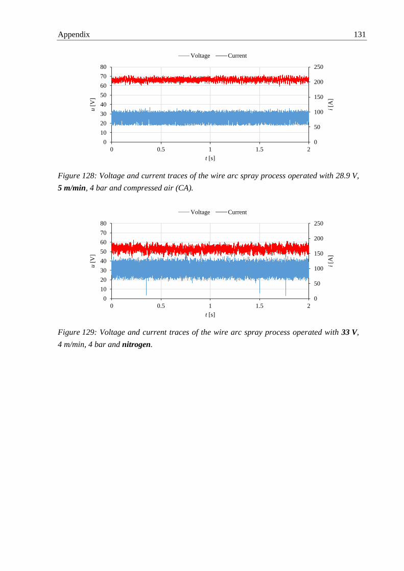
Appendix 131
0
50
100
150
200
250
0
10
20
30
40
50
60
70
80
0 0.5 1 1.5 2
i[A
]
u[V
]
t [s]
Voltage Current
0
50
100
150
200
250
0
10
20
30
40
50
60
70
80
0 0.5 1 1.5 2
i[A
]
u[V
]
t [s]
Voltage Current
Figure 128: Voltage and current traces of the wire arc spray process operated with 28.9 V,
5 m/min, 4 bar and compressed air (CA).
Figure 129: Voltage and current traces of the wire arc spray process operated with 33 V,
4 m/min, 4 bar and nitrogen.

132 Appendix
ffk
0
20
40
60
80
100
120
140
160
180
0
2000
4000
6000
8000
10000
12000
300 400 500 600 700 800 900
Counts
Counts
λ [nm]
0 mm (primary axis) 30 mm (secondary axis) 60 mm (secondary axis)
Figure 130: Spectrum of the wire arc spray process measured at different positions in front
of the wire tips using the spectrometer “ARYELLE”. The blue curve belongs to the primary
axis, the red and green curves to the secondary axis. The process parameters were set to
28.9 V, 4 m/min and 4 bar. Compressed air was used as atomizing gas.
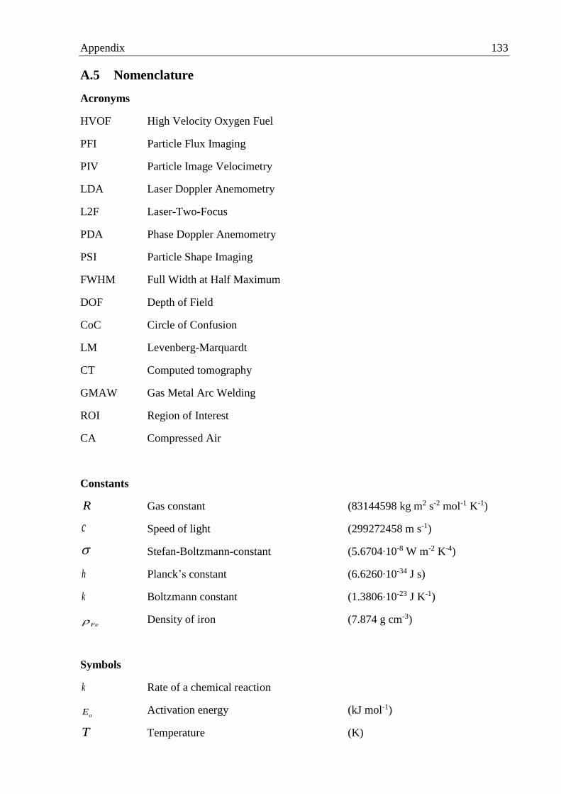
Appendix 133
A.5 Nomenclature
Acronyms
HVOF High Velocity Oxygen Fuel
PFI Particle Flux Imaging
PIV Particle Image Velocimetry
LDA Laser Doppler Anemometry
L2F Laser-Two-Focus
PDA Phase Doppler Anemometry
PSI Particle Shape Imaging
FWHM Full Width at Half Maximum
DOF Depth of Field
CoC Circle of Confusion
LM Levenberg-Marquardt
CT Computed tomography
GMAW Gas Metal Arc Welding
ROI Region of Interest
CA Compressed Air
Constants
R Gas constant (83144598 kg m2 s-2 mol-1 K-1)
c Speed of light (299272458 m s-1)
Stefan-Boltzmann-constant (5.6704∙10-8 W m-2 K-4)
h Planck’s constant (6.6260∙10-34 J s)
k Boltzmann constant (1.3806∙10-23 J K-1)
Fe Density of iron (7.874 g cm-3)
Symbols
k Rate of a chemical reaction
aE Activation energy (kJ mol-1)
T Temperature (K)

134 Appendix
A Frequency factor or surface area (Hz, m2)
Angle (°)
Pf Doppler frequency (Hz)
Pv Particle velocity (m s-1)
Lf Laser frequency (Hz)
L Laser wavelength (nm)
k Wave vector
PMf Doppler shifted frequency (Hz)
Df Doppler-difference frequency (Hz)
, ,x y z Cartesian coordinates (m or Pixel)
dn dt Particle rate (s-1)
Reflectivity
Absorptivity
Transmissivity
Emissivity
P Power (W)
wavelength (nm)
sM Spectral exitance (W m-3)
1C First radiation constant (J m2 s-1)
2C Second radiation constant (m K-1)
M Spectral radiant exitance (W m-3)
1 2, Peak intensity wavelengths (nm)
Q Calculated two-color-pyrometry quotient
mQ Measured two-color-pyrometry quotient
eq Quantum efficiency
1 2,f f Transmission curves of interference filters
GBE Measurement error
1 2, ,I I I Measured or calculated intensities
W Width of the object plane (mm)
H Height of the object plane (mm)

Appendix 135
DOF Depth of field (mm)
,N FD D Nera and far DOF limits (mm)
oS Object distance (mm)
f Focal length (mm)
N f-Number or number of measurements
cd Diameter of the CoC (µm)
w Width of the CCD sensor (Pixel)
h Height of the CCD sensor (Pixel)
G Dimension of an object (mm)
iS Image distance (mm)
B Dimension of an image (mm)
,N FB B Dimension of blurred images (mm)
in the near and far DOF
NX Distance (mm)
1 2,K K Calibration factors (m2 W-1)
K Quotient of the calibration factors
Wavelength step (nm)
0k Proportional factor (m3 W-1)
TH Proportional factor (m3 W-1)
R Sum of square residuals
p Paramter vector
J Jacobi matrix
i Control variable
P Correction vector
Damping term
E Identity matrix
Error vector
,N F Auxiliary matrices
refT Reference temperature (K)
Lv Calibration lamp velocity (cm min-1)

136 Appendix
exp,Et t Exposure time (s)
,1 ,2,ref refI I Average reference values
p Projection value
Projection angle (°)
,iL Integration direction
,f x y 2D intensity distribution
Angle step (°)
k Number of projections directions
n Edge length of a cross section (Pixel)
N Number of cells in a cross section
M Number of projections
,i jw Weight of projection i and cell j
p Projection vector
f Intensity vector
W Weight matrix
m Iteration step
Optical thickness
totI Source intensity
recI Received intensity
ndN dt Particle rate flying through channel n (s-1)
,P nt Time between following particles (s)
Pr Particle radius (µm)
, ,y ,z, ,P x P Pv v v Particle velocity components (m/s)
Pt Particle time pulse (s)
Cl Channel cube edge length (m)
Ct Particle duration of stay in a cube (s)
t Time step (s)
absI Absorbed intensity
PCL Particle overlapping probability
0I Intensity emitted by one particle

Appendix 137
Fe Emissivity of liquid iron
FeO Emissivity of liquid oxidized iron
1, 2,,tot totI I Total measured intensities from particles
flying through a cross section
,iA Luminous area of particle number i (m2)
N Number of particles
flying through a cross section
avgT Average temperature (K)
wv Wire federate (m min-1)
wr Wire radius (mm)
1 2,K K Calibration factors (J-1)
u Voltage (V)
i Electric current (A)
T Time period (s)
massH Energy input per unit mass (J/g)
oxC In-flight oxide content of the particles


![Optical Pyrometry of Fireballs of Metalized Explosives · forrapidinitiationofparticlecombustion[8–13].Whilethe particle dynamics and combustion immediately after the chargedetonationandinthenearfieldhaverecentlybeen](https://img.pdfslide.us/doc/110x75/5f085be27e708231d4219e34/optical-pyrometry-of-fireballs-of-metalized-explosives-forrapidinitiationofparticlecombustion8a13whilethe.jpg)