Tomographic imaging of foam - torus.math.uiuc.edutorus.math.uiuc.edu/jms/Papers/foams/tomogr.pdf · Fig.4.Left. Atypicalimagefromtheexperimentalsetup.Inthiscasetheobjectis acylinderwithneedlesinside.Atransparentplexiglascylinderenclosestheneedles.Published

Tomographic imaging of foam

M.R. Fetterman, E. Tan, L. Ying, R.A, Stack,D.L. Marks, S. Feller, E. Cull, J.M. Sullivan,

D.C. Munson, Jr., S.T. Thoroddsen and D.J. Brady

Beckman Institute, University of Illinois at Urbana-Champaign,Urbana, IL [email protected]

http://www.phs.uiuc.edu

Abstract: The morphology of three-dimensional foams is of interestto physicists, engineers, and mathematicians. It is desired to image the3-dimensional structure of the foam. Many different techniques havebeen used to image the foam, including magnetic resonance imaging,and short-focal length lenses. We use a camera and apply tomographicalgorithms to accurately image a set of bubbles. We correct for thedistortion of a curved plexiglas container using ray-tracing.c© 2000 Optical Society of AmericaOCIS codes: (100.6960) Tomography; (100.6950) Tomographic image processing

References and links1. Denis Weaire, Stefan Hutzler,The Physics of Foams, (Oxford University, Oxford, 1999).2. D. J. Durian, D. A. Weitz, D. J. Pine, “Multiple Light-Scattering Probes of Foam Structure andDynamics,” Science 252 686 (1991).

3. C. Monnereau, M. Vignes-Adler, “Optical Tomography of Real Three-Dimensional Foams,” Jour-nal of Colloid and Interface Science 202 45-53 (1998).

4. C. Monnereau, M. Vignes-Adler, “Dynamics of 3D Real Foam Coarsening,” Phys. Rev. Lett. 80(23) 5228-5231 (1998).

5. C. P. Gonatas, J. S. Leigh, A. G. Yodh, J. A. Glazier, B. Prause,”Magnetic Resonance Images ofCoarsening Inside a Foam,” Phys. Rev. Lett. 75 (3) 573-576 (1995).

6. H.P. Hiriyannaiah, “Computed Tomography for Medical Imaging,” IEEE Signal Processing Mag-azine, 42-59, (March 1997).

7. L.A. Feldkamp, L.C. Davis, J.W. Kress, “Practical Cone-beam Algorithm,” J. Opt. Soc. Am. A1 (6) 612-619 (1984).

8. D. Marks, R.A. Stack, D.J. Brady, D.C. Munson Jr., “Visible Cone-Beam Tomography With aLensless Interferometric Camera,” Science 284 2164-2166 (1999).

9. D.L. Marks, R.A. Stack, D.J. Brady, D.C. Munson Jr., “Cone-beam Tomography with a digitalcamera,” Appl. Opt. (in review) 2000.

10. VTK Toolkit, http://www.kitware.com/vtk.html

11. H.K. Tuy, SIAM J. Appl. Math 43 546 (1983).12. M. Born, E. Wolf, Principles of Optics, (Cambridge University Press, Cambridge, 1980).13. P. Soille, Morphological Image Processing: Principles and Applications, (Springer, Heidelberg,1999).

14. S.A. Koehler, S. Hilgenfeldt, H.A. Stone, “A Generalized View of Foam Drainage: Experimentand Theory,” Langmuir (http://pubs.acs.org/journals/langd5) 16 (15) 6327-6341 (2000).

1 Introduction

Light’s interaction with soap bubbles creates colorful patterns that vividly illustratethe rudimentary principle of wave interference. But there is a lot more to learn aboutsoap bubbles. In a cluster they serve as a model for many cellular systems occurring innature. At low liquid content, they are organized into an intricate network of polyhedralfoam adhering to certain geometric rules discovered by Plateau more than a century ago

(C) 2000 OSA 28 August 2000 / Vol. 7, No. 5 / OPTICS EXPRESS 186#23156 - $15.00 US Received July 19, 2000; Revised August 22, 2000

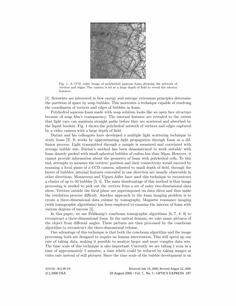
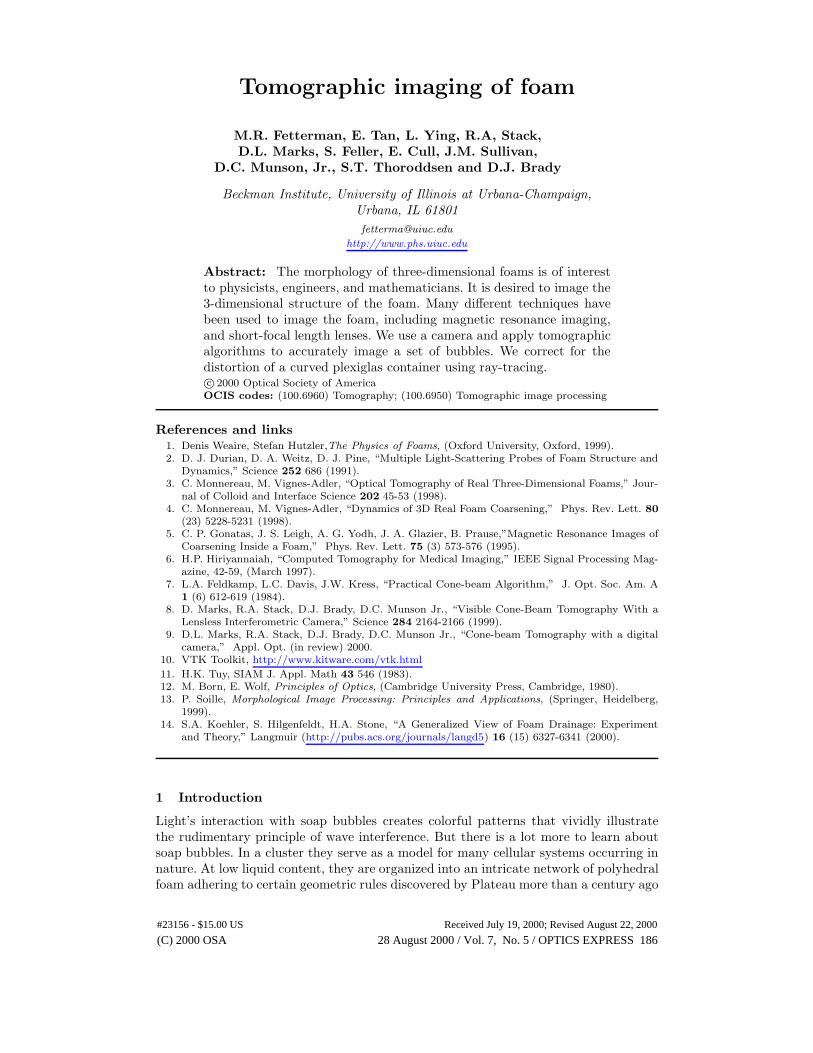
Fig. 1. A CCD video image of polyhedral aqueous foam showing the network ofvertices and edges. The camera is set at a large depth of field to reveal the interiorfeatures.

[1]. Scientists are interested in how energy and entropy extremum principles determinethe partition of space by soap bubbles. This motivates a technique capable of resolvingthe coordinates of vertices and edges of bubbles in foam.

Polyhedral aqueous foam made with soap solution looks like an open face structurebecause of soap film’s transparency. The internal features are revealed to the extentthat light rays can maintain straight paths before they are scattered and absorbed bythe liquid borders. Fig. 1 shows the polyhedral network of vertices and edges capturedby a video camera with a large depth of field.

Durian and his colleagues have developed a multiple light scattering technique tostudy foam [2]. It works by approximating light propagation through foam as a dif-fusion process. Light transmitted through a sample is measured and correlated withaverage bubble size. Durian’s method has been demonstrated to work suitably withfoam densely packed with small spherical bubbles of radius less than 50µm. However, itcannot provide information about the geometry of foam with polyhedral cells. To thisend, attempts to measure the vertices’ position and their connectivity would succeed byscanning a focal plane of a CCD camera, adjusted to small depth of field, through thelayers of bubbles; internal features concealed in one direction are usually observable inother directions. Monnereau and Vignes-Adler have used this technique to reconstructa cluster of up to 50 bubbles [3, 4]. The main disadvantage of this method is that imageprocessing is needed to pick out the vertices from a set of noisy two-dimensional dataslices. Vertices outside the focal plane are superimposed on data slices and thus makethe resolution process difficult. Another approach to the foam imaging problem is tocreate a three-dimensional data volume by tomography. Magnetic resonance imaging(with tomographic algorithms) has been employed to examine the interior of foam withvarious degrees of success [5].

In this paper, we use Feldkamp’s conebeam tomographic algorithms [6, 7, 8, 9] toreconstruct a three-dimensional foam. In the optical domain, we take many pictures ofthe object from different angles. These pictures are then processed by the conebeamalgorithm to reconstruct the three-dimensional volume.

One advantage of this technique is that both the conebeam algorithm and the imageprocessing both are designed to require no human intervention. This will speed up ourrate of taking data, making it possible to analyze larger and more complex data sets.The time scale of this technique is also important. Currently we are taking 1 scan in atime of approximately 5 minutes, a time which could be reduced by taking images atvideo rate instead of still pictures. Since the time scale of the bubble development is on


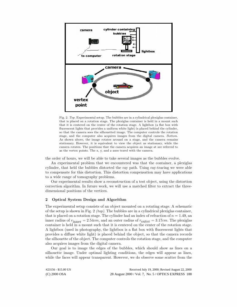
Fig. 2. Top. Experimental setup. The bubbles are in a cylindrical plexiglas container,that is placed on a rotation stage. The plexiglas container is held in a mount suchthat it is centered on the center of the rotation stage. A lightbox (a flat box withfluorescent lights that provides a uniform white light) is placed behind the cylinder,so that the camera sees the silhouetted image. The computer controls the rotationstage, and the computer also acquires images from the digital camera. Bottom.As shown above, the image rotates around on a stage, and the camera remainsstationary. However, it is equivalent to view the object as stationary, while thecamera rotates. The positions that the camera acquires an image at are referred toas the vertex points. The x, y, and z axes travel with the camera.

the order of hours, we will be able to take several images as the bubbles evolve.An experimental problem that we encountered was that the container, a plexiglas

cylinder, that held the bubbles distorted the ray path. Using ray-tracing we were ableto compensate for this distortion. This distortion compensation may have applicationsto a wide range of tomography problems.

Our experimental results show a reconstruction of a test object, using the distortioncorrection algorithm. In future work, we will use a matched filter to extract the three-dimensional positions of the vertices.

2 Optical System Design and Algorithm

The experimental setup consists of an object mounted on a rotating stage. A schematicof the setup is shown in Fig. 2 (top). The bubbles are in a cylindrical plexiglas container,that is placed on a rotation stage. The cylinder had an index of refraction of n = 1.49, aninner radius of rinner = 2.54cm, and an outer radius of router = 3.17cm. The plexiglascontainer is held in a mount such that it is centered on the center of the rotation stage.A lightbox (used in photography, the lightbox is a flat box with fluorescent lights thatprovides a diffuse white light) is placed behind the object, so that the camera recordsthe silhouette of the object. The computer controls the rotation stage, and the computeralso acquires images from the digital camera.

Our goal is to image the edges of the bubbles, which should show as lines on asilhouette image. Under optimal lighting conditions, the edges will appear as lines,while the faces will appear transparent. However, we do observe some scatter from the


Fig. 3. Top. The angular notation used in this paper. Consider a particular voxeland vertex point. We write α for the angle in the vertex plane, β for the anglenormal to the vertex plane, and r for the vector that connects the center of thevertex path to the voxel. Bottom. Angular notation, continued. For a given image,recorded by a camera, Ψy and Ψz refer to the coordinates on the camera. It isnecessary to find a mapping function between the camera coordinates Ψy and Ψz,and the points in the reconstructed voxel space, which are denoted by the angles α,β, and the vector r.

faces of the bubbles.As the object rotates through N steps, an image is taken at each step. Although the

object is rotated, one may picture the object as stationary, and the camera as rotatingabout it Fig. 2 (bottom). Each camera position is referred to as a vertex point Pφ, whereφ describes the angle of the vertex point from the center of the vertex path. The vertexpoints are all in a circle. The algorithms described here do not require a circular vertexpath, but we choose to use one for experimental simplicity. This circle, referred to as thevertex path, lies on the vertex plane. The point V is an arbitrary vertex point, whichwill be referred to later. The axes are defined such that the x,y, and z axes travel withthe camera. The x axis points towards the center of the vertex path [8]. The y axis is inthe vertex plane but normal to the vertex path, and the z axis is normal to the vertexplane.

The angular coordinate notation used in this paper is shown in Fig. 3. Consider acertain voxel, and the angles that it makes with respect to a vertex point such as V .We refer to α as the angle in the vertex plane, and β as the angle normal to the vertexplane. The coordinate r connects the center of the vertex path to the voxel. Note thatfor a given voxel, the values of α and β change, depending on which vertex point we areconsidering, but the value of r remains constant.

For a given image, recorded by a camera, Ψy and Ψz refer to the coordinates on thecamera. These coordinates are not angles, although each value of Ψ does correspondto an angle projecting out from the camera. It is necessary to find a mapping functionbetween the camera coordinates Ψy and Ψz, and the points in the reconstructed voxelspace, which are denoted by the angles α, β, and a distance coordinate.

Typical images are shown in Fig. 4. Fig. 4 (left) shows an image of a test object,


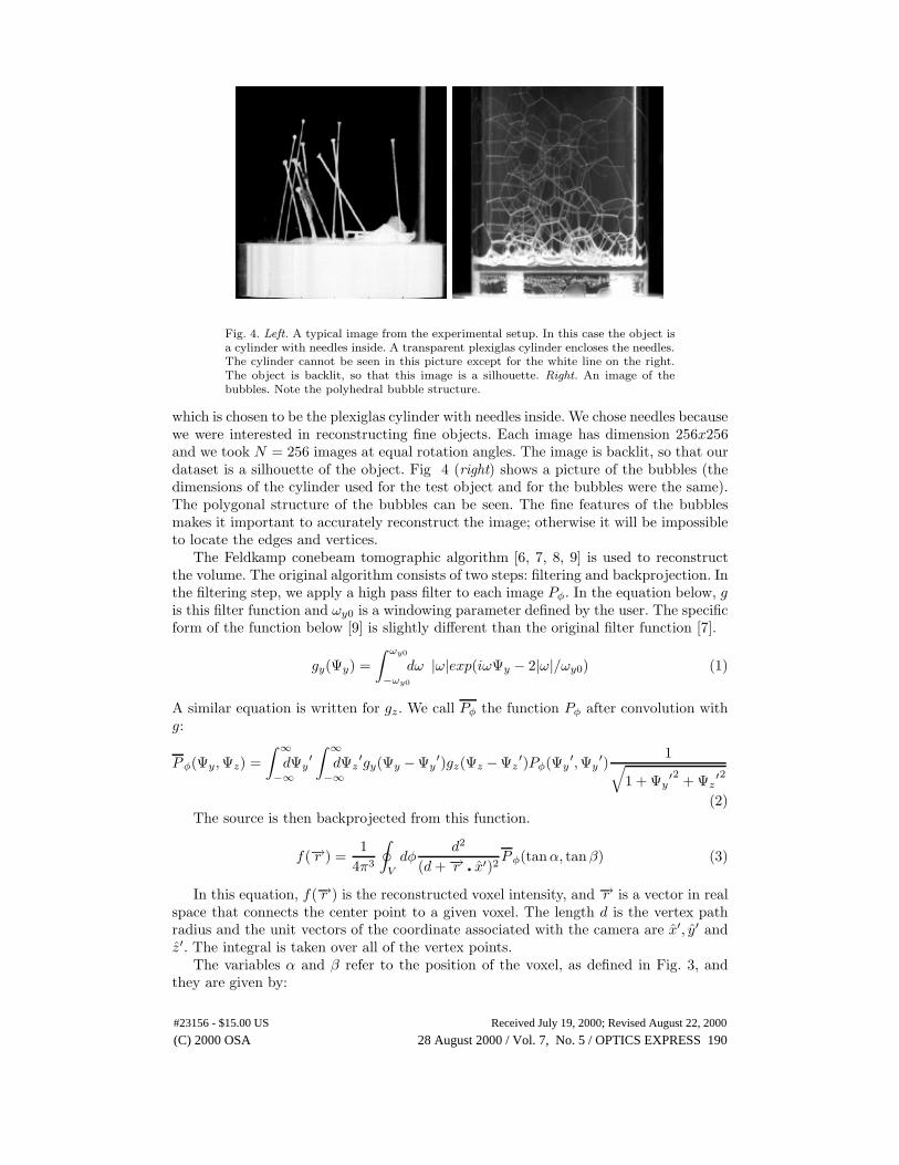
Fig. 4. Left. A typical image from the experimental setup. In this case the object isa cylinder with needles inside. A transparent plexiglas cylinder encloses the needles.The cylinder cannot be seen in this picture except for the white line on the right.The object is backlit, so that this image is a silhouette. Right. An image of thebubbles. Note the polyhedral bubble structure.

which is chosen to be the plexiglas cylinder with needles inside. We chose needles becausewe were interested in reconstructing fine objects. Each image has dimension 256x256and we took N = 256 images at equal rotation angles. The image is backlit, so that ourdataset is a silhouette of the object. Fig 4 (right) shows a picture of the bubbles (thedimensions of the cylinder used for the test object and for the bubbles were the same).The polygonal structure of the bubbles can be seen. The fine features of the bubblesmakes it important to accurately reconstruct the image; otherwise it will be impossibleto locate the edges and vertices.

The Feldkamp conebeam tomographic algorithm [6, 7, 8, 9] is used to reconstructthe volume. The original algorithm consists of two steps: filtering and backprojection. Inthe filtering step, we apply a high pass filter to each image Pφ. In the equation below, gis this filter function and ωy0 is a windowing parameter defined by the user. The specificform of the function below [9] is slightly different than the original filter function [7].

gy(Ψy) =∫ ωy0

−ωy0

dω |ω|exp(iωΨy − 2|ω|/ωy0) (1)

A similar equation is written for gz. We call Pφ the function Pφ after convolution withg:

Pφ(Ψy,Ψz) =∫ ∞

−∞dΨy

′∫ ∞

−∞dΨz

′gy(Ψy −Ψy′)gz(Ψz −Ψz

′)Pφ(Ψy′,Ψy

′)1√

1 + Ψy′2 +Ψz

′2

(2)The source is then backprojected from this function.

f(−→r ) = 14π3

∮V

dφd2

(d+−→r � x′)2Pφ(tanα, tanβ) (3)

In this equation, f(−→r ) is the reconstructed voxel intensity, and −→r is a vector in realspace that connects the center point to a given voxel. The length d is the vertex pathradius and the unit vectors of the coordinate associated with the camera are x′, y′ andz′. The integral is taken over all of the vertex points.

The variables α and β refer to the position of the voxel, as defined in Fig. 3, andthey are given by:


α = arctan−→r � y′

d+−→r � x′ (4)

β = arctan−→r � z′

d+−→r � x′ (5)

We refer to Eq.4 and Eq.5 as the mapping equations, because they define how thethree-dimensional voxel space is to be mapped into the two-dimensional plane of theimage. Writing Eq.3 as the tan of the arctan of the angle in Eq.4 may seem somewhatcircular, but it is convenient to work with the angle α

Eq.3 may be evaluated in two ways: the voxel oriented method or the pixel orientedmethod. In the voxel oriented method, which we use in this paper, every voxel is con-sidered. Then, for each voxel, we sum over all pixels. In the pixel oriented method,the rays originating from each pixel are projected through space, and their intersectionwith the voxel space is calculated. The difference between the voxel-oriented methodand the pixel-oriented method is one of computational preference and convenience only,and does not appear in the Feldkamp equations.

3 Distortion Compensation

Our goal was to image the bubbles, which have very fine features. The bubbles mustbe contained in a cylinder, and this cylinder distorts the light rays. Using ray tracingtechniques. we compensate for this distortion, and recover the correct three-dimensionalreconstruction. First we discuss the approach to compensating for a generalized distor-tion, and then we discuss the specific case of the plexiglas cylinder.

3.1 Distortion compensation for an arbitrary refractive index profile

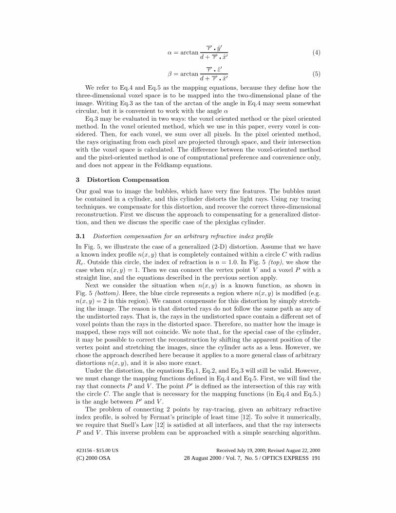
In Fig. 5, we illustrate the case of a generalized (2-D) distortion. Assume that we havea known index profile n(x, y) that is completely contained within a circle C with radiusRc. Outside this circle, the index of refraction is n = 1.0. In Fig. 5 (top), we show thecase when n(x, y) = 1. Then we can connect the vertex point V and a voxel P with astraight line, and the equations described in the previous section apply.

Next we consider the situation when n(x, y) is a known function, as shown inFig. 5 (bottom). Here, the blue circle represents a region where n(x, y) is modified (e.g.n(x, y) = 2 in this region). We cannot compensate for this distortion by simply stretch-ing the image. The reason is that distorted rays do not follow the same path as any ofthe undistorted rays. That is, the rays in the undistorted space contain a different set ofvoxel points than the rays in the distorted space. Therefore, no matter how the image ismapped, these rays will not coincide. We note that, for the special case of the cylinder,it may be possible to correct the reconstruction by shifting the apparent position of thevertex point and stretching the images, since the cylinder acts as a lens. However, wechose the approach described here because it applies to a more general class of arbitrarydistortions n(x, y), and it is also more exact.

Under the distortion, the equations Eq.1, Eq.2, and Eq.3 will still be valid. However,we must change the mapping functions defined in Eq.4 and Eq.5. First, we will find theray that connects P and V . The point P ′ is defined as the intersection of this ray withthe circle C. The angle that is necessary for the mapping functions (in Eq.4 and Eq.5.)is the angle between P ′ and V .

The problem of connecting 2 points by ray-tracing, given an arbitrary refractiveindex profile, is solved by Fermat’s principle of least time [12]. To solve it numerically,we require that Snell’s Law [12] is satisfied at all interfaces, and that the ray intersectsP and V . This inverse problem can be approached with a simple searching algorithm.


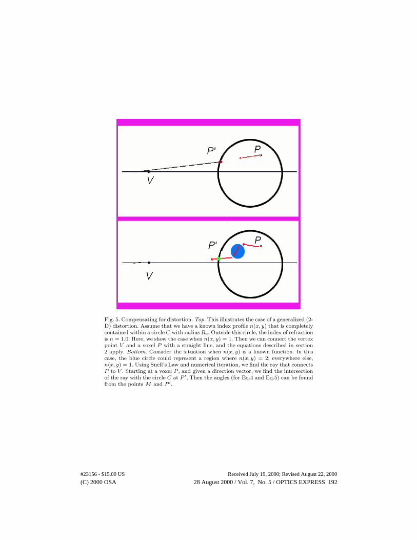
Fig. 5. Compensating for distortion. Top. This illustrates the case of a generalized (2-D) distortion. Assume that we have a known index profile n(x, y) that is completelycontained within a circle C with radiusRc. Outside this circle, the index of refractionis n = 1.0. Here, we show the case when n(x, y) = 1. Then we can connect the vertexpoint V and a voxel P with a straight line, and the equations described in section2 apply. Bottom. Consider the situation when n(x, y) is a known function. In thiscase, the blue circle could represent a region where n(x, y) = 2; everywhere else,n(x, y) = 1. Using Snell’s Law and numerical iteration, we find the ray that connectsP to V . Starting at a voxel P , and given a direction vector, we find the intersectionof the ray with the circle C at P ′, Then the angles (for Eq.4 and Eq.5) can be foundfrom the points M and P ′.


Fig. 6. This shows one step in the construction to find the ray that connects thevoxel to the vertex point. Note that this is a two-dimensional calculation. In thisstep, we project a ray from the voxel towards the vertex point. Using Snell’s law,we find the angle of refraction that occurs when the ray intersects the inner radiusof the cylinder. Not shown is the next step, in which we calculate the refraction ofthe ray at the outer air-cylinder interface.

We start from the voxel, P , and assume a direction vector. We shoot a trial ray intothe volume, and measure the distance between the ray and the vertex point V . Thenwe iterate the initial direction vector until the ray intersects the vertex point.

3.2 Distortion compensation for the specific case of the plexiglas cylinder

The plexiglas cylinder is easy to model because it is an exact circle in the x − y plane.Thus, we can solve for the exact angles, rather than modeling the refractive index profileon a grid. Assume that the cylinder has inner radius R1, outer radius R2, and index ofrefraction n. Because the cylinder has no curvature in the plane normal to the vertexplane, Eq.5 remains unchanged. Eq.4 must be changed because the distortion will alterthe angle α. This is now a two-dimensional problem.

Fig. 6 is a diagram in which we show one step in the construction used to solve forthe ray path. This diagram represents the general case in which we have a voxel withposition −→r inside a circle, and a direction vector. We wish to find the point N ′ at whichthis ray will intersect the circle, as well as the output direction vector. The point N ′ isfound by following the initial direction vector until the circle is intersected. The radiusconnecting N ′ with the center of the circle C makes a 90◦ angle with the tangent to thecircle. Thus, we can find the angle γ, and then using Snell’s Law, find the angle χ. Inthis case we take the inner index of refraction as n1 and the outer index of refraction asn2. Note that we are considering a cylinder with a given thickness, so that we will repeatthis calculation twice. The first time, we will assume that the cylinder has n1 = 1.0 (air)inside, and n2 = 1.49 (plexiglas) outside. The second time, after finding the point N ′,we will then assume that the cylinder has plexiglas inside and air outside. The point atwhich this ray intersects the x-axis is then found.

In Fig. 7, we show a ray tracing diagram with several rays plotted. This representsthe result of the calculation described above, as well as the searching algorithm to find


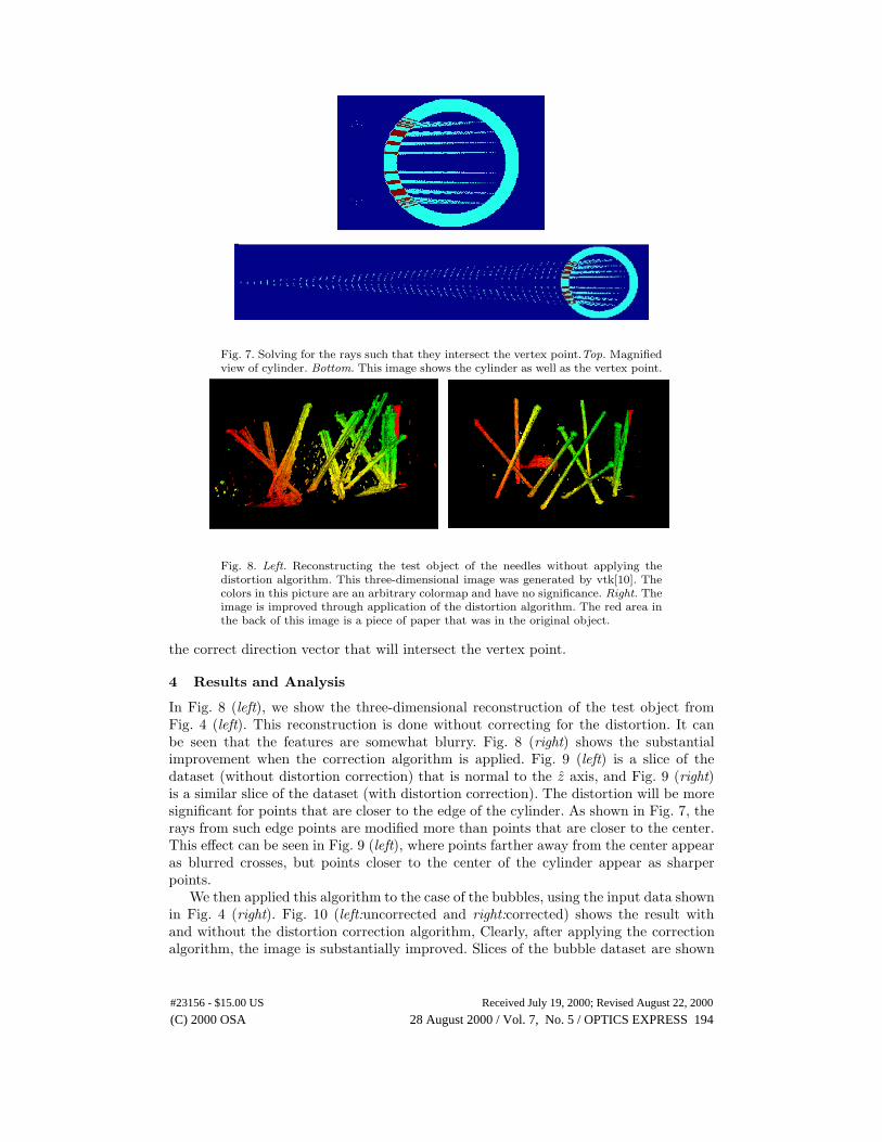
Fig. 7. Solving for the rays such that they intersect the vertex point.Top. Magnifiedview of cylinder. Bottom. This image shows the cylinder as well as the vertex point.

Fig. 8. Left. Reconstructing the test object of the needles without applying thedistortion algorithm. This three-dimensional image was generated by vtk[10]. Thecolors in this picture are an arbitrary colormap and have no significance. Right. Theimage is improved through application of the distortion algorithm. The red area inthe back of this image is a piece of paper that was in the original object.

the correct direction vector that will intersect the vertex point.

4 Results and Analysis

In Fig. 8 (left), we show the three-dimensional reconstruction of the test object fromFig. 4 (left). This reconstruction is done without correcting for the distortion. It canbe seen that the features are somewhat blurry. Fig. 8 (right) shows the substantialimprovement when the correction algorithm is applied. Fig. 9 (left) is a slice of thedataset (without distortion correction) that is normal to the z axis, and Fig. 9 (right)is a similar slice of the dataset (with distortion correction). The distortion will be moresignificant for points that are closer to the edge of the cylinder. As shown in Fig. 7, therays from such edge points are modified more than points that are closer to the center.This effect can be seen in Fig. 9 (left), where points farther away from the center appearas blurred crosses, but points closer to the center of the cylinder appear as sharperpoints.

We then applied this algorithm to the case of the bubbles, using the input data shownin Fig. 4 (right). Fig. 10 (left:uncorrected and right:corrected) shows the result withand without the distortion correction algorithm, Clearly, after applying the correctionalgorithm, the image is substantially improved. Slices of the bubble dataset are shown


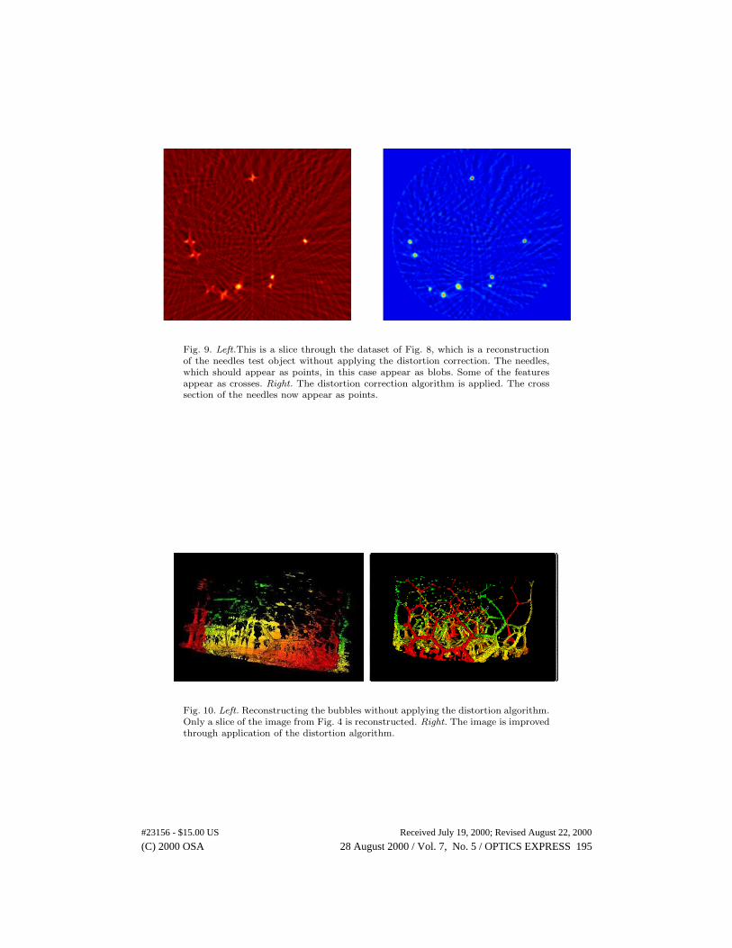
Fig. 9. Left.This is a slice through the dataset of Fig. 8, which is a reconstructionof the needles test object without applying the distortion correction. The needles,which should appear as points, in this case appear as blobs. Some of the featuresappear as crosses. Right. The distortion correction algorithm is applied. The crosssection of the needles now appear as points.

Fig. 10. Left. Reconstructing the bubbles without applying the distortion algorithm.Only a slice of the image from Fig. 4 is reconstructed. Right. The image is improvedthrough application of the distortion algorithm.


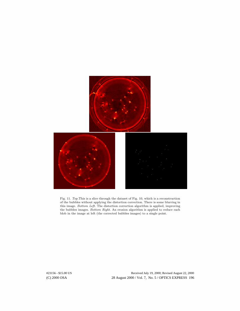
Fig. 11. Top.This is a slice through the dataset of Fig. 10, which is a reconstructionof the bubbles without applying the distortion correction. There is some blurring inthis image. Bottom Left. The distortion correction algorithm is applied, improvingthe bubbles images. Bottom Right. An erosion algorithm is applied to reduce eachblob in the image at left (the corrected bubbles images) to a single point.


in Fig. 11 (top:uncorrected and bottom left:corrected).As in the example of the needles,the closer the points are to the center of the cylinder (in the uncorrected image), theless they are distorted. For studying the foam, it will be important to have a completeset of data that includes the points closest to the cylinder edge, so that this correction isnecessary. The improvement with this correction algorithm seems quite clear, althoughthe corrected image still shows some blurring for points close to the edge of the cylinder.The image may be further improved with image processing. In Fig. 11 (bottom right),we show an erosion [13] algorithm applied to the data of Fig. 11 (bottom left).

5 Conclusions

In this paper we show reconstruction of a three-dimensional foam. The foam is re-constructed using tomography algorithms. Using an algorithm that incorporates raytracing, we are able to compensate for the distortion induced by a plexiglas cylinder. Itis shown that this algorithm improves the images for the case of a test object, as wellas for the bubbles. This distortion correction algorithm may be useful in various areasof tomography.

One area of future work will include improving the initial images. This could includeredesign of the container, with thinner walls, to reduce or eliminate the distortion prob-lem. Although this would improve our foam imaging, it is noted that part of our goalwas to study the computational correction of optical distortion. The illumination of thePlateau borders could also be improved. In [14], the authors dissolve fluorescein salt intheir foaming solution and illuminate with ultra-violet light. With this technique, thePlateau borders fluoresce and there is no stray light.

We are currently analyzing the 3-dimensional data set to reveal the exact polyhedralconfiguration and its evolution. This work includes signal processing techniques such asmatched filtering.

We thank the reviewers for helpful comments. E. Tan, S.T. Thoroddsen, and J.M.Sullivan are supported by NASA Grant NAG3-2122 under the Microgravity FluidPhysics Program.


Documents

Tomographic imaging of foam - torus.math.uiuc.edutorus.math.uiuc.edu/jms/Papers/foams/tomogr.pdf · Fig.4.Left. Atypicalimagefromtheexperimentalsetup.Inthiscasetheobjectis acylinderwithneedlesinside.Atransparentplexiglascylinderenclosestheneedles.Published