Embed Size (px)
Citation preview
Tomographic image quality of rotating slat versus
parallel hole collimated SPECT
Roel Van Holen1 , Steven Staelens1,2, Stefaan Vandenberghe1
1 ELIS Department, MEDISIP, IBBT, Ghent University, IBBT, IBiTech, Ghent,
Belgium2 Molecular Imaging Center Antwerp, Faculty of Medicine, Antwerp University,
Antwerp, Belgium
E-mail: [email protected]
Abstract. Parallel and converging hole collimators are most frequently used in
nuclear medicine. Less common is the use of rotating slat collimators for Single Photon
Emission Computed Tomography (SPECT). The higher photon collection efficiency,
inherent to the geometry of rotating slat collimators results in much lower noise in
the data. However, plane integrals contain spatial information in only one direction,
whereas line integrals provide two-dimensional information. It is not a trivial question
whether the initial gain in efficiency will compensate for the lower information content
in the plane integrals. Therefore, a comparison of the performance of parallel hole and
rotating slat collimation is needed. This study compares SPECT with rotating slat
and parallel hole collimation in combination with MLEM reconstruction with accurate
system modeling and correction for scatter and attenuation. A contrast-to-noise study
revealed an improvement of a factor 2 to 3 for hot lesions and more than a factor of 4 for
cold lesion. Furthermore, a clinically relevant case of heart lesion detection is simulated
for rotating slat and parallel hole collimators. In this case, rotating slat collimators
outperform the traditional parallel hole collimators. We conclude that rotating slat
collimators are a valuable alternative for parallel hole collimators.
1. Introduction
Single Photon Emission Computed Tomography (SPECT) relies on the detection of
gamma rays that result from the decay of radioisotopes, administered to the patient.
Unlike optical photons, high energy photons or gamma rays can not be focussed by
traditional lenses. In order to extract directional information from isotropically emitted
gamma rays, collimators are used instead. Their task is to absorb all photons, not
traveling according to the collimator-imposed direction. As a result, only photons
traveling in the required direction will pass the collimator. A major drawback is that
only a limited amount of photons reach the detector. This low sensitivity typically
results in noisy SPECT images.
The most common collimator used in nuclear medicine is the parallel hole (PH)
collimator. It is constructed as a slab of highly attenuating material (lead or tungsten)
Tomographic image quality of rotating slat versus parallel hole collimated SPECT 2
with a numerous amount of closely packed long, parallel holes. A PH collimator makes
direct one-to-one projection images of the source on the detector. Therefore, the FOV
of a parallel hole collimator is equal to the size of the detector. This property makes
this type of collimator generally applicable in clinical practice. In brain SPECT studies
and sometimes in cardiac studies, the large FOV is not required. Focussing collimators
are then used to obtain higher sensitivity and better spatial resolution. In fan-beam
collimators the holes are tilted toward a focal line while cone-beam collimators have their
holes focussed to a point. Because the focal line of a fan-beam collimator is parallel to
the axis of rotation of the camera, we only have a magnification effect in the transaxial
direction and no magnification in axial direction. On the other hand, projections made
with a conebeam collimator are magnified both in axial and transaxial direction. Finally,
pinhole and multi-pinhole collimators are often used, especially in pre-clinical SPECT
systems. Pinhole-based systems can obtain very good spatial resolution and sensitivity
at the cost of a decreased FOV. All the aforementioned types of collimation however
suffer from the same trade-off between sensitivity, spatial resolution and FOV. For a
discussion on the most common SPECT collimators with respect to these three criteria,
the reader is referred to the excellent overview papers by Wieczorek (Wieczorek and
Goedicke 2006), Accorsi (Accorsi 2006) and Moore (Moore et al 1992).
!"#
$"
!"
#"
$
Figure 1. The geometry of a rotating slat collimator.
Rotating slat (RS) collimators (figure 1), which are the subject of this paper, break
with the traditional collimators described above. They fundamentally differ in the
sense that instead of line integrals, they measure plane integrals. Furthermore, rotating
slat collimators exhibit a different resolution/sensitivity relationship (Vandenberghe et
al 2006). RS collimation has been used in combination with solid state detectors in
the SOLSTICE (SOLid STate Imager with Compact Electronics) design proposed by
Gagnon (Gagnon et al 2001, Griesmer et al 2001). Due to the rotating slat design,
only a limited number of detector elements is required to fill a strip area which reduces
the cost. A similar design has been published by Entine (Entine et al 1979) about 20
years ago, combining a CdTe detector with a parallel plate collimator. Before this, the
Tomographic image quality of rotating slat versus parallel hole collimated SPECT 3
design of a linear detector has been proposed independently by Keyes (Keyes 1975) and
Tosswill (Tosswill 1977). Traditional rectangular SPECT detectors have been studied in
combination with rotating slat collimators by Webb, who found an increased sensitivity
of about a factor of 40 for the rotating slat concept (Webb et al 1992). Due to the
different nature of the data measured by this collimator, other reconstruction techniques
have to be used to reconstruct images. Analytic reconstruction methods for planar
and tomographic acquisitions have been derived by Lodge (Lodge et al 1995, Lodge et
al 1996). A 3D iterative reconstruction algorithm for the SOLSTICE camera has been
proposed by Wang (Wang et al 2004) and by Zeng (Zeng et al 2003).
A drawback of reconstructing plane integral data measured by a rotating slat collimator,
to 3D images is the much longer computation time needed compared to a parallel hole
reconstruction. This problem was solved in an earlier paper with the development
of a reconstruction method that uses two updates per iteration, one in plane integral
space and one in sinogram space (Van Holen et al 2007). Among different MLEM
implementations to reconstruct plane integral data, this method was found to be the
fastest. Furthermore, it maintains image quality.
Planar RS imaging with Filtered Back-Projection (FBP) reconstruction has previously
been studied by Lodge (Lodge et al 1995). Their work shows an advantage in signal-to-
noise ratio (SNR) over a PH collimator for sparse activity distributions and an enhanced
contrast in small hot spots. A previous comparison of planar image quality, using
accurate system modeling in an iterative reconstruction, indicates improved contrast-
to-noise ratios up to a factor 3, even in large objects approaching the size of the field-
of-view (FOV) of the camera (Van Holen et al 2008). In the tomographic case, FBP
reconstructed SPECT images with a RS collimator again confirmed improved noise
characteristics for small objects (smaller than 10 cm) and showed improved contrast only
for small regions of high tracer uptake (Lodge et al 1996). In (Wang et al 2004), next to
better hot spot contrast, also an increased contrast was found for cold lesions. However,
in this study, the SOLSTICE detector was used and the image quality improvement
was not only due to collimation with slats but also due to the combined effect of small
detector width, better collimator resolution and solid state detector material. Moreover,
in this comparison, no model for depth-dependent detector blurring was used in the
reconstruction. Finally, in (Zhou et al 2010), where analytical collimator models were
used, a comparable performance of PH and RS collimation was found, depending on
object size and object distance.
In this paper, realistic measurements are simulated and all detector and collimator
parameters will be matched in order to make a comparison between RS and PH
collimation. This also implies that an attenuating medium will be present and accurately
modeled. Therefore, we first need to validate whether classical scatter and attenuation
correction techniques can be applied to plane integral reconstruction. After the
development of an appropriate attenuation correction technique for the tomographic
image reconstruction of plane integral data, we will compare image quality to a parallel
hole collimator with identical field-of-view by means of a contrast-to-noise analysis.
Tomographic image quality of rotating slat versus parallel hole collimated SPECT 4
Next, a realistic Tc-99m-MIBI scan will be simulated on both a SPECT scanner
equipped with RS and PH collimators to demonstrate the use of slat collimation in
clinical practice.
Tomographic image quality of rotating slat versus parallel hole collimated SPECT 5
2. Materials and Methods
2.1. Monte Carlo simulation models
Geant4 Application for Tomographic Emission (GATE) (Santin et al 2003) was used to
simulate the rotating slat and the parallel hole acquisitions. The detector was identical
for both systems and was modeled as a pixelated solid state detector consisting of
192×192 individual CdZnTe (CZT) pixels of 1.8 mm×1.8 mm. The thickness of the
CZT was set to 5 mm. The energy resolution of the CZT was set to 5% at 140keV. To
make the efficiency of the detector independent of the collimator type, the active area
of one pixel was set to be only 1.5 mm×1.5 mm. With g = 1.5 mm, the collimator septa
have a width of 0.3 mm thickness.
The RS collimator of figure 1 was simulated as 193 parallel lead slats of height
h = 40 mm, placed in between two neigbouring pixel rows. The thickness of a slat was set
to 0.3 mm while the length was equal to the length W of the detector (W = 345.6 mm).
The PH collimator had the same height and thickness as the RS collimator and was
matched to the pixelated detector. This resulted in a parallel hole collimator with
square holes of 1.5 mm×1.5 mm. The collimator resolution is thus matched for both
collimators and is 5 mm at 10 cm collimator distance. The RS collimator/detector
(a) (b)
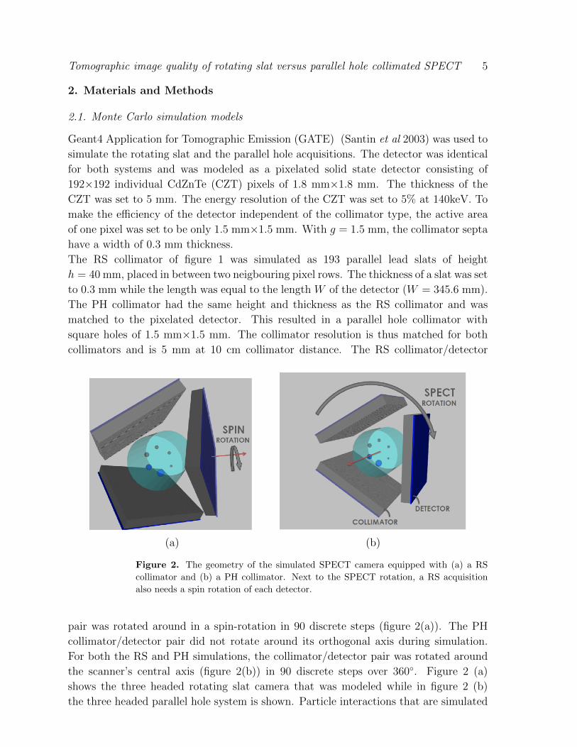
Figure 2. The geometry of the simulated SPECT camera equipped with (a) a RS
collimator and (b) a PH collimator. Next to the SPECT rotation, a RS acquisition
also needs a spin rotation of each detector.
pair was rotated around in a spin-rotation in 90 discrete steps (figure 2(a)). The PH
collimator/detector pair did not rotate around its orthogonal axis during simulation.
For both the RS and PH simulations, the collimator/detector pair was rotated around
the scanner’s central axis (figure 2(b)) in 90 discrete steps over 360◦. Figure 2 (a)
shows the three headed rotating slat camera that was modeled while in figure 2 (b)
the three headed parallel hole system is shown. Particle interactions that are simulated
Tomographic image quality of rotating slat versus parallel hole collimated SPECT 6
include photo-electric effect, Compton and Raleigh scattering, electron ionization and
Bremsstrahlung.
2.2. Scatter estimation
The Dual Energy Window (DEW) scatter estimation technique (Koral et al 1990) was
used to correct for scatter in both the data acquired with a RS collimator and the PH
collimator. According to this method, the scatter estimate is calculated as follows:
gEST = k
(gSW
wMW
wSW
), (1)
with gSW the data measured in the scatter window. Since Tc-99m will be used
throughout this study, the width of our main energy window wMW was chosen 14 keV
around 140 keV and wSW , the width of the scatter window was chosen 10 keV and was
located around 125 keV.
To investigate whether the DEW scatter correction technique will also be valid for RS
collimation, two cylindrical phantoms filled with Tc-99m in water, were simulated in
GATE. Their respective diameters were 20 cm and 35 cm, while their height was fixed at
20 cm. The rotation radius (distance from center of rotation to collimator) was 17.5 cm
and 22.5 cm respectively. The respective activities were 3.7 MBq and 11.3 MBq while
13.5 minutes of acquisition time were simulated. Both cylinders were placed in the
center of the field of view and aligned with the scanner’s central axis.
Thanks to the history tracking of the detected events, GATE flags every detection that
scattered in the phantom. Consequently, the true scatter distribution gTRUE is known.
In order to study the feasibility of a spectral based scatter estimation correction, we
looked at the energy spectra of respectively PH collimated data and RS collimated
data. For both the small and large cylinder, detections originating from a spherical
region with 10 cm diameter in the center of the phantom were selected to generate
an energy spectrum. To study the spatial dependency of the spectrum also detections
originating from a spherical region at a peripheral position, offset from the center by
10 cm in both transaxial dimensions and by 5 cm along the scanner’s central axis, were
selected in the large cylinder to generate a third energy spectrum. For comparison, the
three spectra were generated for both PH and RS. As a quantitative validation, the
estimated scatter fraction was compared to the true scatter fraction. No attempt is
made to make a validation of spatial distributions at the level of the projections.
2.3. Attenuation correction
2.3.1. Implementation Since the data are affected by attenuation, we need a method to
compensate for the loss of photons at larger depths. An attenuation correction method
which fully models the attenuation along each possible ray of projection as used by
Zeng et al. (Zeng et al 1991) is used for the reconstruction of the PH data. However,
for RS data, this method is only possible in a fully 3D reconstruction algorithm which
directly maps image to the plane integrals using one single system matrix. Since our
Tomographic image quality of rotating slat versus parallel hole collimated SPECT 7
!"##$%&'()*$+',)--./+$'01&2')3'4$&$56)%'
70.%'#)&16)%'
(a)
(b)
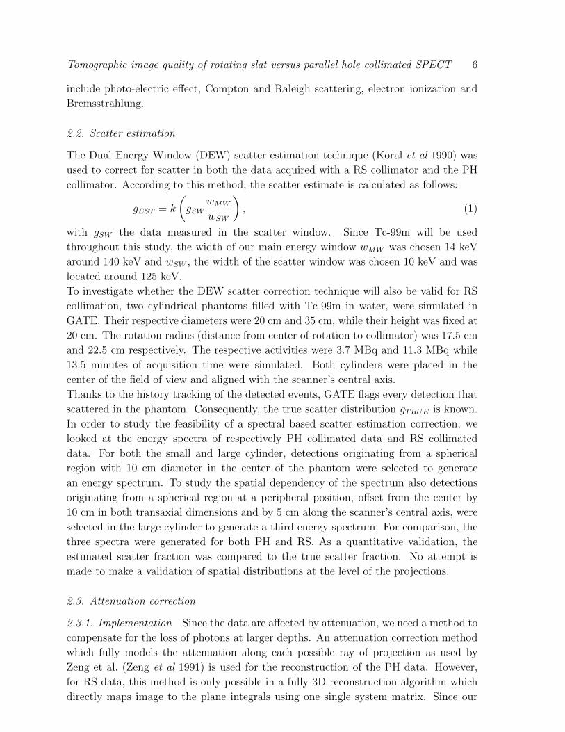
Figure 3. (a) One of the possible paths along which attenuation has to be calculated.
This calculation needs to be repeated for every path in the fan, for every voxel, every
spin and every SPECT angle. (b) The sensitivity weighted intersection lengths for all
possible paths of detection for one voxel at one spin angle.
reconstruction method splits the system matrix in two separate ones, the original paths
of detection are lost and this method can not be applied. Furthermore, tracing every
possible ray for every spin and SPECT angle would be too tedious. Therefore, we base
ourselves on Chang’s attenuation correction method (Chang 1978) which calculates an
average attenuation factor at each voxel. However, where Chang calculates the mean
attenuation value over all SPECT angles for every voxel, our method will calculate an
average attenuation coefficient c over all spin angles φ for every voxel (x, y, z) and for
Tomographic image quality of rotating slat versus parallel hole collimated SPECT 8
every SPECT angle θ:
c(x, y, z, θ) = (1
Φ
Φ∑i=0
exp(−(ML)φi)−1, (2)
with (ML)φi the mean attenuation-length product for spin angle φi. The calculation of
(ML)φi was done by tracing 100 paths connecting the voxel of interest with equidistant
points, sampling the detector. In figure 3 (a) one of such paths is displayed. The ray
tracing, using Siddon’s algorithm (Siddon 1985), returned the intersection lengths of
these rays with the attenuation image voxels. Sensitivity weighting of the intersection
lengths with cos3 α, with α the incidence angle, yielded a map of weighted intersection
lengths for a certain voxel (figure 3 (b)). Finally, multiplication with the µ value of the
intersected voxel and averaging over all possible paths resulted in (ML)φi .
Since our system matrix rotates the image according to the appropriate SPECT
angle before applying sensitivity and resolution modeling, we can use the factors c to
compensate the rotated image for attenuation. In this way, an approximate attenuation
compensation is performed, calculated with every SPECT angle as an average over all
spin angles.
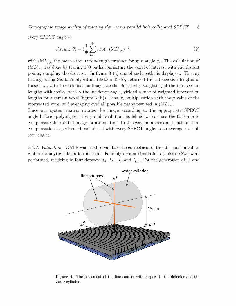
2.3.2. Validation GATE was used to validate the correctness of the attenuation values
c of our analytic calculation method. Four high count simulations (noise<0.8%) were
performed, resulting in four datasets Id, Id,0, Iy and Iy,0. For the generation of Id and
Figure 4. The placement of the line sources with respect to the detector and the
water cylinder.
Tomographic image quality of rotating slat versus parallel hole collimated SPECT 9
Iy, line sources aligned with respectively the d- and y-axis of the scanner (figure 4)
were simulated with a cylindrical water phantom present. The camera was spun over
360 degrees. Binning the recorded data according to the source position resulted in the
datasets Id and Iy. Id,0 and Iy,0 were generated in a similar way with the only difference
being the absence of the water cylinder. Since the detector was rotated over all spin
angles there exists the following relation between datasets I and I0:
I = I01
Φ
Φ∑i=0
exp(−(ML)φi)), (3)
II0
should thus be equal to the reciprocal of the attenuation values c.
A validation at the level of reconstructed images is also performed by simulating a
dataset with and without attenuating medium. The XCAT software phantom (Segars
et al 2010) was used to simulate a clinically realistic measurement of a patient injected
with Tc-99m-MIBI, used for the assessment of heart perfusion and/or viability. For
the purpose of investigating the attenuation correction, the XCAT simulation was
performed, once without and once with the XCAT attenuation map presents. The
images were then reconstructed first without and then with attenuation correction. The
reconstruction of the simulated dataset without attenuation present served as the gold
standard image and the reconstructed dataset with attenuation is reconstructed without
and with attenuation correction. Both of these latter reconstructions are then compared
to the gold standard. For reference, this study was performed with both PH and RS
collimation. More details on the XCAT simulation can be found in section 2.6 while
image reconstruction is detailed in the next section (2.4).
2.4. Image reconstruction
Image reconstruction of the PH data was performed with plain MLEM, including
attenuation correction as proposed by Zeng et al. (Zeng et al 1991) . Scatter correction
is performed by adding gEST to the forward projection at each MLEM iteration.
For the purpose of reconstruction of the plane integral data collected by the RS
collimator, we used a previously proposed split-matrix method for accelerated image
reconstruction (Van Holen et al 2007), (Zeng and Gagnon 2004). This method does
not model the process to go from plane integrals to image in one single step, but splits
the process in two separate steps. The process of plane integration is thus split in two
subsequent line integrations. The first line integration to go from sinograms to plane
integral data is modeled by A and the second (matrix B) models the step to go from
image to sinograms. The resulting system matrix AB is used in an MLEM algorithm:
f̂kt+1
=f̂kt∑
iBki
∑j Aij
∑i
Bki
∑j
Aijgj∑
iAij∑
k Bkif̂kt+ gEST
. (4)
The following iterative process is followed by this algorithm: in a first step, an initial
image estimate f̂kt
is forward projected with system matrix B to a sinogram estimate.
Next, this sinogram estimate is forward projected using A. For the purpose of scatter
Tomographic image quality of rotating slat versus parallel hole collimated SPECT 10
correction, gEST is added to the forward projection. This final forward projection is
compared to the plane integral data gj. The resulting plane integral update is projected
backward using At and immediately projected backward with Bt to image space where it
serves as an update image. After updating and normalizing the original image estimate,
the next iteration can start.
In the first part of the system matrix (B), which transforms image space to sinogram
space, we model the depth dependent sensitivity as the mean sensitivity in a plane
parallel to the detector. Furthermore, depth dependent resolution is also modeled in
B. Attenuation compensation is also applied at this level. System matrix A involves
a mapping from sinogram to plane integral space. At this level, we do not include any
sensitivity modeling nor resolution modeling. No regularisation, inter-update filtering
or post-filtering was applied in any of the reconstructions.
2.5. Monte Carlo simulations of realistic acquisitions
2.5.1. Image quality phantom For the purpose of a contrast-to-noise comparison, the
image quality phantom (Standard Jaszczak PhantomTM), shown in figure 2 is simulated
containing 4 hot spheres (diameters: 9.9 mm, 12.4 mm, 15.4 mm, 19.8 mm) and two
cold spheres (diameters: 24.8 mm and 31.3 mm). The activity concentration is set in
order to have a sphere-to-background activity ratio of 8:1 in the hot spheres. The total
activity in the phantom was 370 Mbq. The phantom is simulated to be filled with water
with an attenuation coefficient µ of 0.154 cm−1 at 140 keV. For the purpose of noise
calculation, ten realizations of each dataset were simulated. The rotation radius of the
detector was 15 cm and the acquisition time was set to 8 minutes.
2.5.2. Influence of system modeling The data generated by the Monte Carlo simulation
resulted in a one dataset for RS and one for PH. For image reconstruction, we use the
algorithm of equation 4. The data are all reconstructed with attenuation correction as
explained in section 2.4. In order to investigate the influence of resolution and sensitivity
modeling in the system matrix, the two datasets are reconstructed in three different
ways: (i) without any modeling, thus using a simple line integral model (no model); (ii)
with resolution modeling (RM) and (iii) both with resolution and sensitivity modeling
(RSM). Since for a PH collimator the sensitivity is constant over the FOV, reconstruction
RM and RSM will produce equal results. Image quality is then investigated on the basis
of contrast recovery and noise. The hot- and cold spot contrast recovery are defined
as (Kessler et al 1984):
CRC(%) =
ml−mb
mb
C − 1× 100 (5)
with C being the real contrast in the phantom, in our case C = 8 for the hot spots
and C = 0 for the cold spots. ml and mb are the mean lesion and background activity,
averaged over ten realizations. The noise coefficient (%) is calculated as
NC(%) =σpmp
× 100. (6)
Tomographic image quality of rotating slat versus parallel hole collimated SPECT 11
Here, σp and mp respectively are the pixel standard deviation and pixel mean throughout
ten realizations of the simulation, averaged over all pixels in a background region of
interest.
We evaluated the cold and hot lesion contrast recovery, CRCc and CRCh, averaged over
respectively the two cold and the four hot lesions at a NC of 25%.
2.5.3. Image quality improvement After investigating the influence of using an accurate
system model orthogonal slices through the 3D images, reconstructed with the RM
method, will be shown for both the PH and RS collimator at equal NC. Also, 1D
profiles through the lesions will be drawn. Next, the contrast-to-noise was plotted for all
lesions to investigate the contrast-to-noise properties. This will especially be interesting
to study the convergence properties. For the PH acquisition, the same simulation as
described before is repeated in order to study the difference in imaging time to reach
equal contrast-to-noise behavior for both collimators.
2.6. Simulation of a realistic Tc99m-MIBI scan
The XCAT software was used to simulate a measurement of a patient injected with Tc-
99m-MIBI. Realistic organ uptake values which have been published before have been
used (Jaszczak et al 1996). Background, lungs, liver and heart-wall respectively were
assigned activity concentrations of 0.0075 MBq/ml, 0.0048 MBq/ml, 0.07 MBq/ml and
0.15 MBq/ml. One defect (2.8 ml) was simulated in the left ventricular anterolateral wall
with an activity concentration of 0.0075 MBq/ml. Total activity in the XCAT phantom
was 49 MBq. The PH and RS scanners were modeled as described in section 2.1, with
the only difference of rotation radius (23 cm) and acquisition time (810 seconds). The
data were binned for PH in 96×96 detector bins for 90 SPECT bins while the RS data
were binned in 96 detector bins, 90 SPECT and 90 spin angle bins. The rotation radius
was 23 cm. Since the lesion is simulated, we know the exact location of where it should
be in the reconstructed images. Therefore, the simulated lesion location is chosen as
the lesion ROI (ROIl). A reference region of interest is chosen in the anteroseptal wall
in order to calculate the CRC. Noise is calculated in a background region of interest in
the lungs.
3. Results
3.1. Scatter Estimation
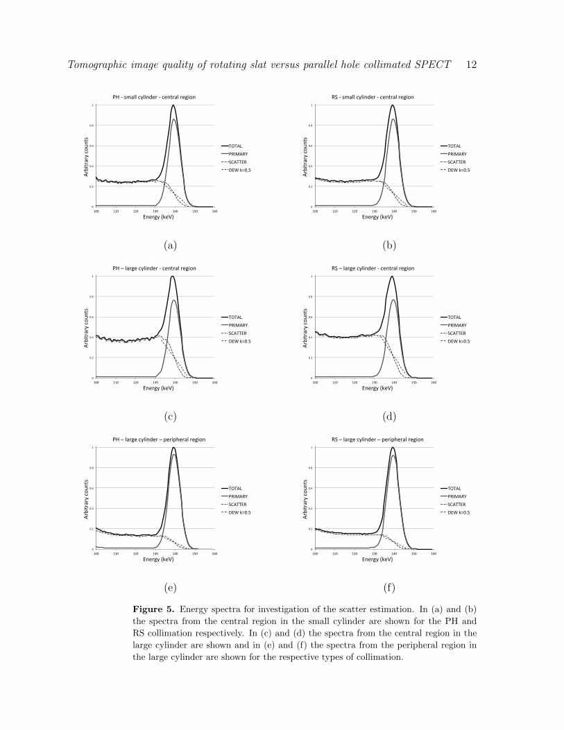
In figure 5 the spectra for the central regions in the small (figure 5 (a) and (b)) and
large cylinder (figure 5 (c) and (d)) are shown together with the spectra obtained for
the peripheral region in the large cylinder (figure 5 (e) and (f)) for both the PH and RS
collimator. A study of these spectra shows that the spectral distribution of scattered
photons for the RS collimator are comparable to the PH collimated scatter distribution.
A comparison of the estimated scatter fraction to the true scatter fraction in table 1
Tomographic image quality of rotating slat versus parallel hole collimated SPECT 12
!"
!#$"
!#%"
!#&"
!#'"
("
(!!" ((!" ($!" ()!" (%!" (*!" (&!"
+,+-."
/012-03"
45-++60"
768"9:!;*"
PH -‐ small cylinder -‐ central region
Energy (keV)
Arbitrary coun
ts
!"
!#$"
!#%"
!#&"
!#'"
("
(!!" ((!" ($!" ()!" (%!" (*!" (&!"
+,+-."
/012-03"
45-++60"
768"9:!#*"
RS -‐ small cylinder -‐ central region
Energy (keV)
Arbitrary coun
ts
(a) (b)
!"
!#$"
!#%"
!#&"
!#'"
("
(!!" ((!" ($!" ()!" (%!" (*!" (&!"
+,+-."
/012-03"
45-++60"
768"9:!#*"
PH – large cylinder -‐ central region
Energy (keV)
Arbitrary coun
ts
!"
!#$"
!#%"
!#&"
!#'"
("
(!!" ((!" ($!" ()!" (%!" (*!" (&!"
+,+-."
/012-03"
45-++60"
768"9:!#*"
RS – large cylinder -‐ central region
Energy (keV)
Arbitrary coun
ts
(c) (d)
!"
!#$"
!#%"
!#&"
!#'"
("
(!!" ((!" ($!" ()!" (%!" (*!" (&!"
+,+-."
/012-03"
45-++60"
768"9:!#*"
PH – large cylinder – peripheral region
Energy (keV)
Arbitrary coun
ts
!"
!#$"
!#%"
!#&"
!#'"
("
(!!" ((!" ($!" ()!" (%!" (*!" (&!"
+,+-."
/012-03"
45-++60"
768"9:!#*"
RS – large cylinder – peripheral region
Energy (keV)
Arbitrary coun
ts
(e) (f)
Figure 5. Energy spectra for investigation of the scatter estimation. In (a) and (b)
the spectra from the central region in the small cylinder are shown for the PH and
RS collimation respectively. In (c) and (d) the spectra from the central region in the
large cylinder are shown and in (e) and (f) the spectra from the peripheral region in
the large cylinder are shown for the respective types of collimation.
Tomographic image quality of rotating slat versus parallel hole collimated SPECT 13
learns that the error made by the DEW scatter estimation technique makes small errors
which are comparable for PH and RS.
PH RS
True Estimated True Estimated
small central 21.8 22.6 21.9 22.7
large central 33.4 32.7 33.8 35.0
large peripheral 11.7 12.2 12.8 13.1
Table 1. Comparison of ectimated and true scatter fractions (%)
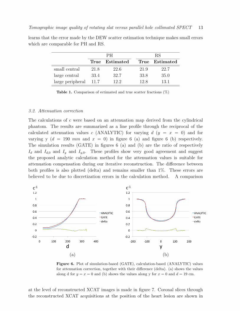
3.2. Attenuation correction
The calculations of c were based on an attenuation map derived from the cylindrical
phantom. The results are summarized as a line profile through the reciprocal of the
calculated attenuation values c (ANALYTIC) for varying d (y = x = 0) and for
varying y (d = 190 mm and x = 0) in figure 6 (a) and figure 6 (b) respectively.
The simulation results (GATE) in figures 6 (a) and (b) are the ratio of respectively
Id and Id,0 and Iy and Iy,0. These profiles show very good agreement and suggest
the proposed analytic calculation method for the attenuation values is suitable for
attenuation compensation during our iterative reconstruction. The difference between
both profiles is also plotted (delta) and remains smaller than 1%. These errors are
believed to be due to discretization errors in the calculation method. A comparison
(a) (b)
Figure 6. Plot of simulation-based (GATE), calculation-based (ANALYTIC) values
for attenuation correction, together with their difference (delta). (a) shows the values
along d for y = x = 0 and (b) shows the values along y for x = 0 and d = 19 cm.
at the level of reconstructed XCAT images is made in figure 7. Coronal slices through
the reconstructed XCAT acquisitions at the position of the heart lesion are shown in
Tomographic image quality of rotating slat versus parallel hole collimated SPECT 14
!"#$%&!'$("!# !"#$%&#'()*+&(,%+'-%..*-,%+'
(a) (b)
!"#$%&'()*&+,)%-,..(-+,)%
!"
!#$"
!#%"
!#&"
!#'"
!#("
!#)"
!#*"
!#+"
!#,"
$"
!" (!" $!!" $(!" %!!" %(!" &!!" &(!"
-./0"12340350"
67"
4."67"
!"#$%"&'(()*
+",(-.$/0
1*2"3&
4#*
(c) (d)
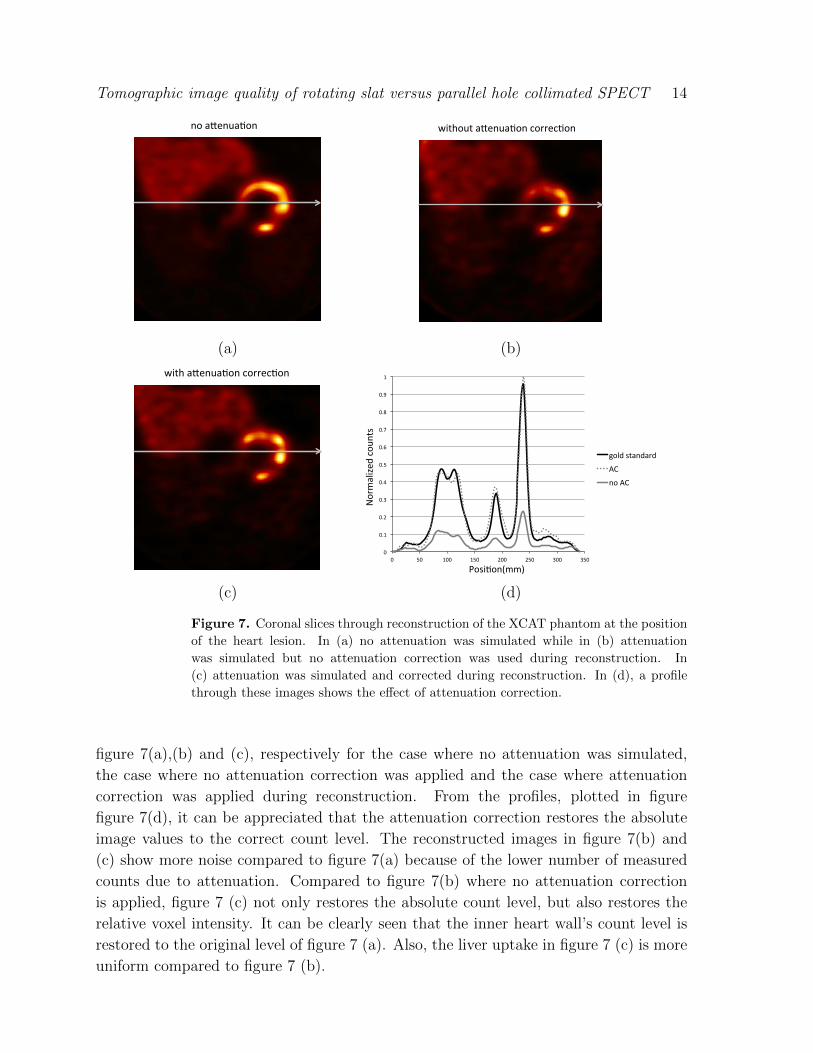
Figure 7. Coronal slices through reconstruction of the XCAT phantom at the position
of the heart lesion. In (a) no attenuation was simulated while in (b) attenuation
was simulated but no attenuation correction was used during reconstruction. In
(c) attenuation was simulated and corrected during reconstruction. In (d), a profile
through these images shows the effect of attenuation correction.
figure 7(a),(b) and (c), respectively for the case where no attenuation was simulated,
the case where no attenuation correction was applied and the case where attenuation
correction was applied during reconstruction. From the profiles, plotted in figure
figure 7(d), it can be appreciated that the attenuation correction restores the absolute
image values to the correct count level. The reconstructed images in figure 7(b) and
(c) show more noise compared to figure 7(a) because of the lower number of measured
counts due to attenuation. Compared to figure 7(b) where no attenuation correction
is applied, figure 7 (c) not only restores the absolute count level, but also restores the
relative voxel intensity. It can be clearly seen that the inner heart wall’s count level is
restored to the original level of figure 7 (a). Also, the liver uptake in figure 7 (c) is more
uniform compared to figure 7 (b).
Tomographic image quality of rotating slat versus parallel hole collimated SPECT 15
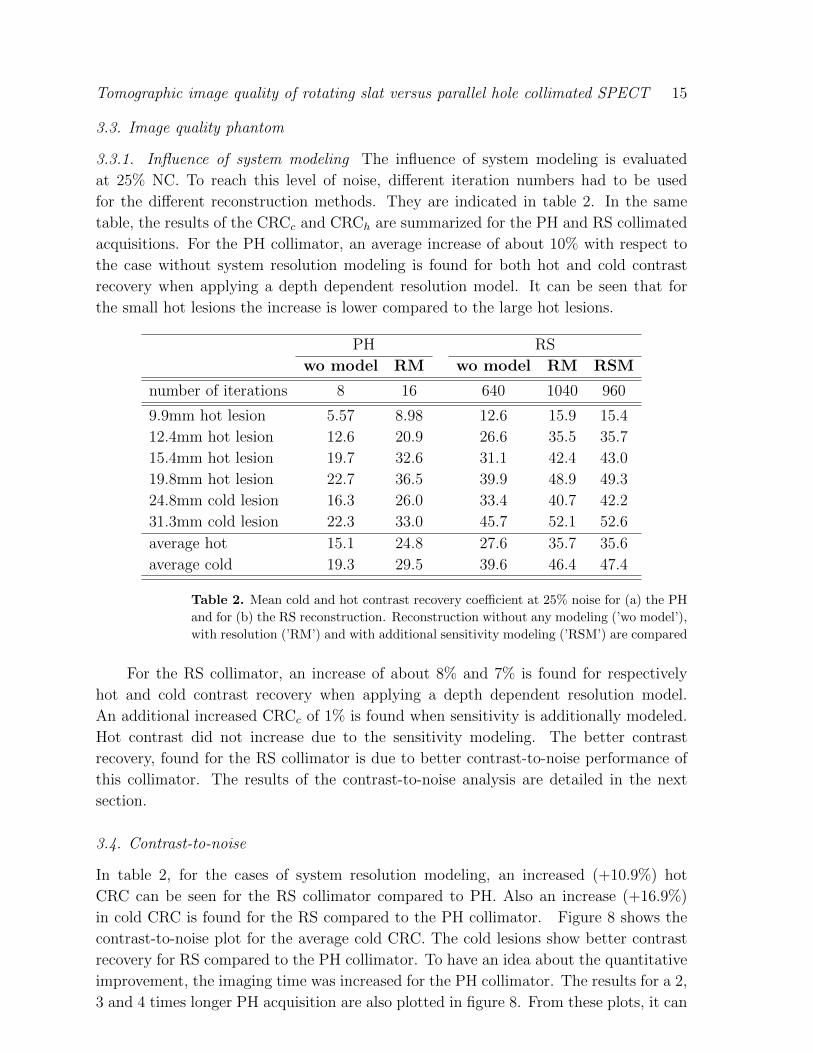
3.3. Image quality phantom
3.3.1. Influence of system modeling The influence of system modeling is evaluated
at 25% NC. To reach this level of noise, different iteration numbers had to be used
for the different reconstruction methods. They are indicated in table 2. In the same
table, the results of the CRCc and CRCh are summarized for the PH and RS collimated
acquisitions. For the PH collimator, an average increase of about 10% with respect to
the case without system resolution modeling is found for both hot and cold contrast
recovery when applying a depth dependent resolution model. It can be seen that for
the small hot lesions the increase is lower compared to the large hot lesions.
PH RS
wo model RM wo model RM RSM
number of iterations 8 16 640 1040 960
9.9mm hot lesion 5.57 8.98 12.6 15.9 15.4
12.4mm hot lesion 12.6 20.9 26.6 35.5 35.7
15.4mm hot lesion 19.7 32.6 31.1 42.4 43.0
19.8mm hot lesion 22.7 36.5 39.9 48.9 49.3
24.8mm cold lesion 16.3 26.0 33.4 40.7 42.2
31.3mm cold lesion 22.3 33.0 45.7 52.1 52.6
average hot 15.1 24.8 27.6 35.7 35.6
average cold 19.3 29.5 39.6 46.4 47.4
Table 2. Mean cold and hot contrast recovery coefficient at 25% noise for (a) the PH
and for (b) the RS reconstruction. Reconstruction without any modeling (’wo model’),
with resolution (’RM’) and with additional sensitivity modeling (’RSM’) are compared
For the RS collimator, an increase of about 8% and 7% is found for respectively
hot and cold contrast recovery when applying a depth dependent resolution model.
An additional increased CRCc of 1% is found when sensitivity is additionally modeled.
Hot contrast did not increase due to the sensitivity modeling. The better contrast
recovery, found for the RS collimator is due to better contrast-to-noise performance of
this collimator. The results of the contrast-to-noise analysis are detailed in the next
section.
3.4. Contrast-to-noise
In table 2, for the cases of system resolution modeling, an increased (+10.9%) hot
CRC can be seen for the RS collimator compared to PH. Also an increase (+16.9%)
in cold CRC is found for the RS compared to the PH collimator. Figure 8 shows the
contrast-to-noise plot for the average cold CRC. The cold lesions show better contrast
recovery for RS compared to the PH collimator. To have an idea about the quantitative
improvement, the imaging time was increased for the PH collimator. The results for a 2,
3 and 4 times longer PH acquisition are also plotted in figure 8. From these plots, it can
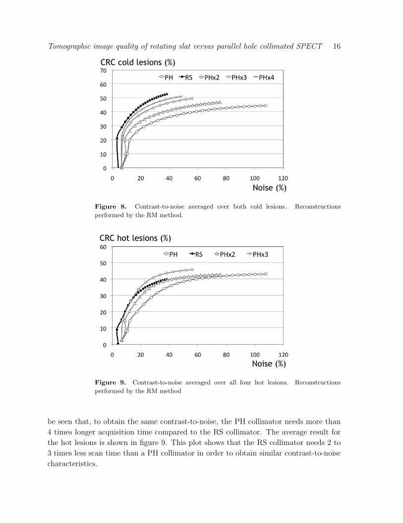
Tomographic image quality of rotating slat versus parallel hole collimated SPECT 16
CRC cold lesions (%)
Noise (%)
Figure 8. Contrast-to-noise averaged over both cold lesions. Reconstructions
performed by the RM method.
CRC hot lesions (%)
Noise (%)
Figure 9. Contrast-to-noise averaged over all four hot lesions. Reconstructions
performed by the RM method
be seen that, to obtain the same contrast-to-noise, the PH collimator needs more than
4 times longer acquisition time compared to the RS collimator. The average result for
the hot lesions is shown in figure 9. This plot shows that the RS collimator needs 2 to
3 times less scan time than a PH collimator in order to obtain similar contrast-to-noise
characteristics.
Tomographic image quality of rotating slat versus parallel hole collimated SPECT 17
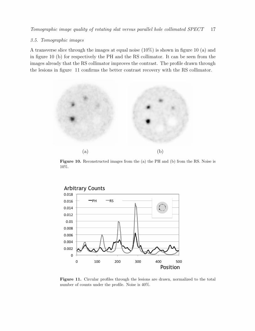
3.5. Tomographic images
A transverse slice through the images at equal noise (10%) is shown in figure 10 (a) and
in figure 10 (b) for respectively the PH and the RS collimator. It can be seen from the
images already that the RS collimator improves the contrast. The profile drawn through
the lesions in figure 11 confirms the better contrast recovery with the RS collimator.
(a) (b)
Figure 10. Reconstructed images from the (a) the PH and (b) from the RS. Noise is
10%.
Arbitrary Counts
Position
Figure 11. Circular profiles through the lesions are drawn, normalized to the total
number of counts under the profile. Noise is 40%.
Tomographic image quality of rotating slat versus parallel hole collimated SPECT 18
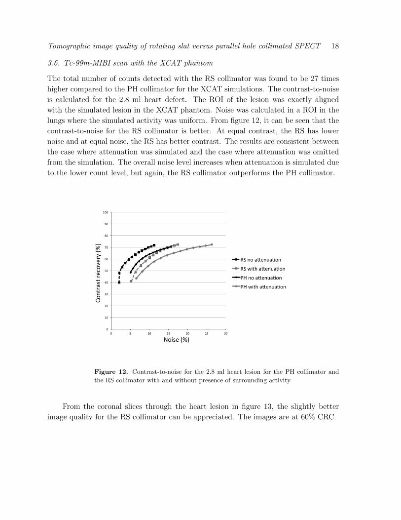
3.6. Tc-99m-MIBI scan with the XCAT phantom
The total number of counts detected with the RS collimator was found to be 27 times
higher compared to the PH collimator for the XCAT simulations. The contrast-to-noise
is calculated for the 2.8 ml heart defect. The ROI of the lesion was exactly aligned
with the simulated lesion in the XCAT phantom. Noise was calculated in a ROI in the
lungs where the simulated activity was uniform. From figure 12, it can be seen that the
contrast-to-noise for the RS collimator is better. At equal contrast, the RS has lower
noise and at equal noise, the RS has better contrast. The results are consistent between
the case where attenuation was simulated and the case where attenuation was omitted
from the simulation. The overall noise level increases when attenuation is simulated due
to the lower count level, but again, the RS collimator outperforms the PH collimator.
!"
#!"
$!"
%!"
&!"
'!"
(!"
)!"
*!"
+!"
#!!"
!" '" #!" #'" $!" $'" %!"
,-"./"012.304/."
,-"5678"012.304/."
9:"./"012.304/."
9:"5678"012.304/."
Noise (%)
Contrast re
covery (%
)
Figure 12. Contrast-to-noise for the 2.8 ml heart lesion for the PH collimator and
the RS collimator with and without presence of surrounding activity.
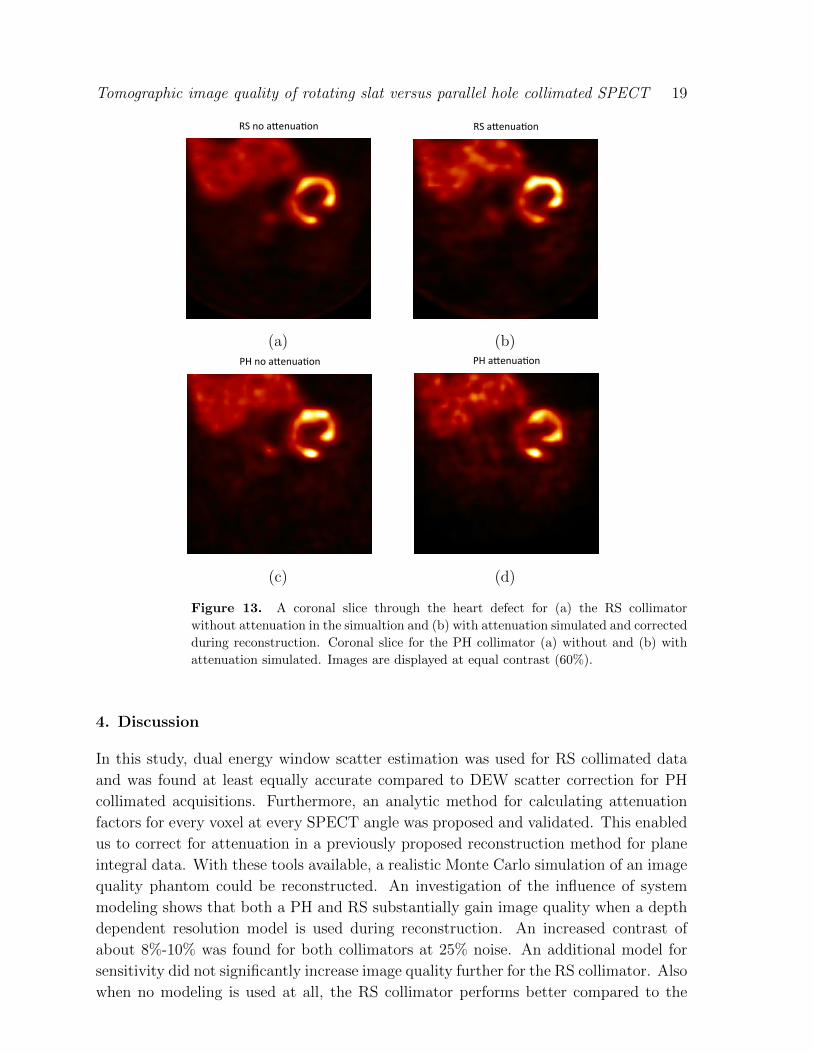
From the coronal slices through the heart lesion in figure 13, the slightly better
image quality for the RS collimator can be appreciated. The images are at 60% CRC.
Tomographic image quality of rotating slat versus parallel hole collimated SPECT 19
!"#$%#&'($)&*%$# !"#$%&'($)*'#
(a) (b)!"#$%#&'($)&*%$# !"#$%&'($)*'#
(c) (d)
Figure 13. A coronal slice through the heart defect for (a) the RS collimator
without attenuation in the simualtion and (b) with attenuation simulated and corrected
during reconstruction. Coronal slice for the PH collimator (a) without and (b) with
attenuation simulated. Images are displayed at equal contrast (60%).
4. Discussion
In this study, dual energy window scatter estimation was used for RS collimated data
and was found at least equally accurate compared to DEW scatter correction for PH
collimated acquisitions. Furthermore, an analytic method for calculating attenuation
factors for every voxel at every SPECT angle was proposed and validated. This enabled
us to correct for attenuation in a previously proposed reconstruction method for plane
integral data. With these tools available, a realistic Monte Carlo simulation of an image
quality phantom could be reconstructed. An investigation of the influence of system
modeling shows that both a PH and RS substantially gain image quality when a depth
dependent resolution model is used during reconstruction. An increased contrast of
about 8%-10% was found for both collimators at 25% noise. An additional model for
sensitivity did not significantly increase image quality further for the RS collimator. Also
when no modeling is used at all, the RS collimator performs better compared to the
Tomographic image quality of rotating slat versus parallel hole collimated SPECT 20
PH collimator (20% higher cold contrast and 12% higher contrast at 25% noise). These
findings are consistent with the findings of Wang (Wang et al 2004). The improvements
found by Lodge (Lodge et al 1996), where FBP was used as a reconstruction algorithm,
were more modest. Therefore, we believe that it is not the modeling, but the nature of
MLEM, which includes a statistical model of the data, that favors the RS collimation.
While in FBP, all noisy projections are simply backprojected and added in image space
for every spin and every SPECT angle, MLEM tries to find a maximum likelihood
solution by iteratively correcting an initial estimate with a smooth correction term.
The contrast-to-noise investigation shows that SPECT images obtained with a rotating
slat collimator in combination with iterative reconstruction and accurate modeling
provide a better contrast-to-noise trade-off compared to images obtained with an
equivalent PH collimator. In terms of imaging time, equal average cold contrast-to-
noise is found in a more than 4 times shorter scan time for the RS collimated detector.
For the contrast-to-noise, averaged over the hot lesions, the results show a 2 to 3 times
improvement in terms of acquisition time. This study thus not only shows better hot
spot contrast recovery, which was also found by Lodge (Lodge et al 1996), but also
proves better cold spot contrast recovery, which is consistent with the results obtained
by Wang (Wang et al 2004). These results were obtained however with a slat collimated
solid-state strip detector, but in that study, no depth dependent resolution was modeled
and no attenuation compensation was used. Also, it was unclear whether the improved
contrast-to-noise was due to the better solid state detector or due to the slat collimator.
This study indicates the improvement is due to the collimator. We need to note however
that an effective sensitivity gain could be lower when more detectors are used or when
smaller rotation radii are possible. Due to the extra rotation needed by the RS design,
more space is needed compared to a PH system with equal size detectors not to let the
detectors run in to each other while spinning.
The case study of the Tc-99m-MIBI scan with the XCAT phantom shows that in a
clinical setting, where a larger scan radius has to be used and where there is more
activity throughout the FOV, the RS collimator still reaches better image quality.
5. Conclusion
In this paper, an attenuation correction method for the reconstruction of plane integral
data was developed in order to study the tomographic image quality with respect to
a parallel hole collimator. Furthermore, a standard scatter correction method was
validated. For a standard image quality phantom, better image quality was obtained
for both hot and cold lesions. In the clinically realistic case of a Tc-99m-MIBI scan
of a heart defect, the rotating slat collimator also obtains better images. Therefore,
tomographic rotating slat is an interesting alternative for existing collimation.
Tomographic image quality of rotating slat versus parallel hole collimated SPECT 21
Acknowledgments
Research funded by a the Fund for Scientific Research Flanders (FWO, Belgium) and
by the Ghent University.
References
Accorsi R 2006 High-efficiency, high-resolution SPECT techniques for cardiac imaging Proceedings of
Science .
Chang L 1978 A method for attenuation correction in radionuclide computed tomography IEEE
Transactions on Nuclear Science 25 638–643.
Entine G, Luthmann R, Mauderli W, Fitzgerald L, Williams C and Tosswill C 1979 Cadmium Telluride
gamma camera IEEE Transactions on Nuclear Science 26 552–558.
Gagnon D, Zeng G, Links M, Griesmer J and Valentino F 2001 in ‘Nuclear Science Symposium
Conference Record’ Vol. 2 pp. 1156–1160.
Griesmer J, Kline B, Grosholz J, Parnham K and Gagnon D 2001 in ‘Nuclear Science Symposium
Conference Record’ Vol. 2 pp. 1050–1054.
Jaszczak R, Gilland D, McConnick J, Scarfone C and Coleman R 1996 The effect of truncation reduction
in fan beam transmission for attenuation correction of cardiac SPECT IEEE Transactions on
Nuclear Science 43 2255–2262.
Kessler R, Ellis J and Eden M 1984 Analysis of tomographic scan data: limitations imposed by
resolution and background Journal of Computer Assisted Tomography 8 514–22.
Keyes W 1975 Correspondence: The fan-beam gamma camera Physics in Medicine and Biology 20 489–
493.
Koral K, Swailem F, Buchbinder S, Clinthorne N, Rogers W and Tsui B 1990 SPECT dual-energy-
window Compton correction: scatter multiplier required for quantification. Journal of Nuclear
Medicine 31 90–98.
Lodge M, Binnie D, Flower M and Webb S 1995 The experimental evaluation of a prototype rotating
slat collimator for planar gamma camera imaging Physics in Medicine and Biology 40 427–448.
Lodge M, Webb S, Flower M and Binnie D 1996 A prototype rotating slat collimator for single photon
emission computed tomography IEEE Transactions on Medical Imaging 15 500–511.
Moore S, Kouris K and Cullum I 1992 Collimator design for single photon emission tomography
European Journal of Nuclear Medicine 19 138–150.
Santin G, Strul D, Lazaro D, Simon L, Krieguer M, Vieira Martins M, Breton V and Morel C 2003
GATE, a Geant4-based simulation platform for PET and SPECT integrating movement and
time management IEEE Transactions on Nuclear Science 50 1516–1521.
Segars W, Sturgeon G, Mendonca S, Grimes J and Tsui B 2010 4D XCAT phantom for multimodality
imaging research Medical Physics 37 4902–4915.
Siddon R 1985 Fast calculation of the exact radiological path for a three-dimensional CT array. Medical
Physics 12 252–255.
Tosswill C 1977 Computerized rotating laminar collimation imaging system US patent application 646
(granted December 1977) pp. 917–967.
Van Holen R, Vandenberghe S, Staelens S and Lemahieu I 2007 Fast 3D image reconstruction for
rotating slat collimated gamma cameras. Proceedings 9th International Meeting on Fully Three-
Dimensional Image Reconstruction in Radiology and Nuclear Medicine pp. 390–392.
Van Holen R, Vandenberghe S, Staelens S and Lemahieu I 2008 Comparing planar image quality of
rotating slat and parallel hole collimation: influence of system modeling Physics in Medicine
and Biology 53 1989–2002.
Vandenberghe S, Staelens S, Byrne C L, Soares E J, Lemahieu I and Glick S J 2006 Reconstruction of
Tomographic image quality of rotating slat versus parallel hole collimated SPECT 22
2d pet data with monte carlo generated system matrix for generalized natural pixels. Physics
in Medicine and Biology 51 3105–3125.
Wang W, Hawkins W and Gagnon D 2004 3D RBI-EM reconstruction with spherically-symmetric basis
function for SPECT rotating slat collimator Physics in Medicine and Biology 49 2273–2292.
Webb S, Binnie D, Flower M and Ott R 1992 Monte Carlo modeling of the performace of a rotating
slit collimator for improved planar gamma camera imaging Physics in Medicine and Biology
37 1095–1108.
Wieczorek H and Goedicke A 2006 Analytical model for SPECT detector concepts IEEE Transactions
on Nuclear Science 53 1102–1112.
Zeng G, Gagnon D, Natterer F, Wang W, Wrinkler M and Hawkins W 2003 Local tomography property
of residual minimization reconstruction with planar integral data IEEE Transactions on Nuclear
Science 50.
Zeng G, Gullberg G, Tsui B and Terry J 1991 Three-dimensional iterative reconstruction algorithms
with attenuation and geometric point response correction IEEE Transactions on Nuclear Science
38 693–702.
Zeng G L and Gagnon D 2004 Image reconstruction algorithm for a SPECT system with a convergent
rotating slat collimator IEEE Transactions on Nuclear Science 51 142–148.
Zhou L, Defrise M, Vunckx K and Nuyts J 2010 Comparison between parallel hole and rotating
slat collimation: Analytical noise propagation models IEEE Transactions on Medical Imaging
29 2038–2052.