Tomislav Globan Vladimir Ar Petar Sorić Inflation in New EU …web.efzg.hr/repec/pdf/Clanak 14-05.pdf · · 2014-10-23importance of domestic vs. foreign inflation determinants

F E B – W O R K I N G P A P E R S E R I E S 1 4 - 0 5

Page 1 of 31

J. F. Kennedy sq. 6 10000 Zagreb, Croatia Tel +385(0)1 238 3333

http://www.efzg.hr/wps [email protected]

WORKING PAPER SERIES

Paper No. 14-05

Tomislav Globan

Vladimir Arčabić Petar Sorić

Inflation in New EU Member States: A Domestically or

Externally Driven Phenomenon?

http://www.efzg.hr/wps

mailto:[email protected]

http://www.efzg.hr/default.aspx

http://www.unizg.hr/


Page 2 of 31

Inflation in New EU Member States: A Domestically or Externally Driven

Phenomenon?

Tomislav Globan [email protected]

Faculty of Economics and Business University of Zagreb Trg J. F. Kennedy 6

10 000 Zagreb, Croatia

Vladimir Arčabić [email protected]

Faculty of Economics and Business University of Zagreb

Trg J. F. Kennedy 6 10 000 Zagreb, Croatia

Petar Sorić

[email protected] Faculty of Economics and Business

University of Zagreb Trg J. F. Kennedy 6

10 000 Zagreb, Croatia

The views expressed in this working paper are those of the author(s) and not necessarily represent those of the Faculty of Economics and Business – Zagreb. The paper has not undergone formal review or approval. The paper is published to

bring forth comments on research in progress before it appears in final form in an academic journal or elsewhere.

Copyright October 2014 by Tomislav Globan, Vladimir Arčabić & Petar Sorić All rights reserved.

Sections of text may be quoted provided that full credit is given to the source.





Page 3 of 31

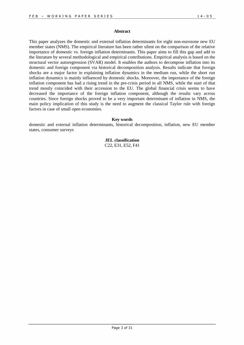
Abstract

This paper analyzes the domestic and external inflation determinants for eight non-eurozone new EU

member states (NMS). The empirical literature has been rather silent on the comparison of the relative

importance of domestic vs. foreign inflation determinants. This paper aims to fill this gap and add to

the literature by several methodological and empirical contributions. Empirical analysis is based on the

structural vector autoregression (SVAR) model. It enables the authors to decompose inflation into its

domestic and foreign component via historical decomposition analysis. Results indicate that foreign

shocks are a major factor in explaining inflation dynamics in the medium run, while the short run

inflation dynamics is mainly influenced by domestic shocks. Moreover, the importance of the foreign

inflation component has had a rising trend in the pre-crisis period in all NMS, while the start of that

trend mostly coincided with their accession to the EU. The global financial crisis seems to have

decreased the importance of the foreign inflation component, although the results vary across

countries. Since foreign shocks proved to be a very important determinant of inflation in NMS, the

main policy implication of this study is the need to augment the classical Taylor rule with foreign

factors in case of small open economies.

Key words

domestic and external inflation determinants, historical decomposition, inflation, new EU member

states, consumer surveys

JEL classification

C22, E31, E52, F41


Page 4 of 31

1. Introduction

During the Great Moderation period, inflation was rather stable in the vast majority of developed

countries. At the same time, the emerging economies of Central and Eastern Europe (CEE) frequently

recorded even double-digit inflation figures (see e.g. Hammermann and Flanagan (2009) for an

overview of inflation differentials in CEE countries). The necessity of thorough inflation analysis in

those countries has been even more accentuated with regards to recent economic developments.

Namely, Vašíček (2009) as well as Franta, Saxa and Šmídková (2010) provide fresh evidence that

inflation persistence in some New EU Member States (NMS) is much higher than in the eurozone

economies. As they suggest, this may lead to severe problems with fulfilling the Maastricht criterion

on inflation. Additionally, almost all NMS have witnessed a growth in total external trade relative to

GDP during the crisis period. This has made their economies more vulnerable to external shocks in the

global economic conditions (demand-pull inflation) or in commodity prices (cost-push inflation).

However, the empirical literature has been rather silent on the comparison of the relative importance

of domestic vs. foreign factors driving inflation. One of the rare empirical studies of that kind is

Mihailov, Rumler and Scharler (2011a), who make an effort to estimate the New Keynesian Phillips

curve (NKPC) for 10 OECD countries using the Generalized Method of Moments (GMM). The

authors start from the Galí and Monacelli (2005) open-economy NKPC model (comprising inflation

expectations, output gap and the effective terms of trade vis-à-vis the rest of the world), and consider

several alternative model specifications. For the majority of the observed countries, the external

factors (terms of trade) turned out to be more important for inflation than the domestic one (output

gap).

To the best of the authors’ knowledge, the only study formally comparing the relevance of domestic

and external inflation drivers in the CEE economies is the one by Mihailov, Rumler and Scharler

(2011b). They estimate the NKPC for 12 NMS (within the 2004 and 2007 enlargements), repeating the

exact same empirical exercise as in Mihailov, Rumler and Scharler (2011a). Their results strongly

point out the superiority of the original Galí and Monacelli (2005) model, which also enables the

comparison of the relative importance of domestic factors (output gap) and foreign determinants

(terms of trade) in explaining the inflation generating process. The authors obtain rather diverse

results, explicating them by the size effect. Namely, the domestic inflation component is found to be

dominant in the four largest sample countries (Poland, Hungary, the Czech Republic and Bulgaria).

On the other hand, the majority of the remaining (mostly smaller) countries exhibit a mainly

externally-driven inflation generating process.

This paper analyzes the domestic and external inflation determinants for eight non-eurozone NMS:

Bulgaria, Croatia, the Czech Republic, Hungary, Latvia, Lithuania, Poland, and Romania. It aims to

shed some light on the underexplored phenomenon of NMS inflation and contribute to “revealing”

inflation either as a dominantly domestically or externally driven phenomenon in small open

economies.

This study adds to the literature by several methodological and empirical contributions. First of all, it

comprises a much wider set of explanatory variables than the NKPC framework of Mihailov, Rumler

and Scharler (2011b). To be specific, several domestic variables (inflation expectations, output gap,

M1, and the nominal effective exchange rate) and external factors (eurozone output gap, EURIBOR

and Brent Crude oil price) are considered. Second, Mihailov, Rumler and Scharler (2011b) base their

analysis on a static NKPC regression, inspecting the importance of domestic and external inflation

determinants by mere comparison of their estimated regression coefficients. Contrary to that, this

paper bases its empirical analysis on the structural vector autoregression (SVAR) model, enabling the

authors to examine the temporal interdependence of the observed variables. The aggregate domestic

and external inflation components are extracted through the forecast error variance decomposition.

The link between each of the two components and actual inflation is examined through the historical

decomposition and rolling-window correlations.

The existing studies of the inflation generating process in NMS have been criticized due to short

macroeconomic time series, which poses the question of their results' robustness (Benkovskis 2008).


Page 5 of 31

The robustness issue has been even more scrutinized due to exogenous shocks such as the EU

accession or the recent Great Recession. It is precisely the rolling-window correlation analysis within

the SVAR model which enables the researcher to investigate the possible effect of the above

mentioned extreme events on the relevance of domestic/external inflation components. Additionally, it

enables the researcher to analyze whether the relative importance of the two inflation components is

stable in the analyzed period, or has the relationship been altered by the process of economic

integration with the EU, trade openness and international competition.

Results of this analysis indicate that foreign shocks are a major factor in explaining inflation dynamics

in the medium run in the majority of the analyzed NMS, while the short run inflation dynamics is

mainly under the influence of domestic shocks. Moreover, the importance of the foreign inflation

component in most NMS started to rise in the mid-2000s, coinciding with the time those countries

joined the EU. The global financial crisis seems to have decreased the importance of the foreign

inflation component, although the results vary across countries. Since foreign shocks proved to be very

important in driving inflation in NMS, the main policy implication of this study is the need to augment

the classical Taylor rule with foreign factors in case of small open economies.

The paper is conceptualized as follows. Section 2 offers a brief review of the prevailing inflation

theories and the main inflation determinants they point to. Section 3 presents the analyzed dataset and

the applied SVAR methodology, thoroughly explaining the identified structural relationships between

the observed variables. Section 4 reveals the obtained empirical results. Finally, section 5 provides

concluding remarks.

2. Theoretical aspects and literature review

Modern macroeconomic models almost unavoidably employ the NKPC as the workhorse model for

any kind of inflation analysis. Therefore this study also starts from the following NKPC specification:

1

~ tttt Ey (1)

where t is the actual inflation rate, is the output gap, is the output elasticity to marginal cost,

1ttE stands for inflation expectations, while and are the model parameters.1

The above NKPC model has often been augmented in the literature by several domestic and external

variables. The following section offers an overview on the main theoretical underpinnings and the

relevant empirical findings regarding the “geographical” segregation of inflation sources.

2.1. The global output gap hypothesis

The traditional approach to modeling inflation is country-centric. It postulates that the actual inflation

rate is a derivative of the domestic economic conditions (excess demand/economic slack), while the

external influences are modeled solely by the exchange rate or import prices (Borio and Filardo 2007).

However, the empirical literature in the last decade has altered the prevailing paradigm to a globe-

centric one, fully acknowledging the inflation sensitivity to global economic conditions. Borio and

Filardo (2007) augment the Phillips curve by global output gap for as many as 15 industrialized

countries and find strong evidence in favor of the globalization effect. This finding is not firmly

corroborated by other studies. For instance, Calza (2009), inter alia, reviews the voluminous literature

on this topic. The author stresses that the global output gap has mostly not been found significant for

the US inflation, just as for the OECD countries (Pain et al. 2006; Ihrig et al. 2007).

1 Technical details and the full derivation of NKPC can be found in e.g. Galí and Gertler (1999).


Page 6 of 31

However, the impact of global output gap on inflation in emerging economies (particularly the CEE

ones analyzed in this study) is still an underexplored phenomenon. This paper aims to fill that niche.

2.2. Exchange rate pass-through effect

The exchange rate pass-through (ERPT) is defined as the exchange rate influence on domestic

inflation. The mechanism itself is rather straightforward: exchange rate appreciation directly causes

the import prices to fall and export prices to rise. The final effect on the aggregate domestic price level

depends on various factors. For example, Takhtamanova (2010) pinpoints four main factors

determining the ERPT extent: the degree of openness of the economy, the fraction of flexible-price

firms, central bank credibility, and the degree of ERPT at the microeconomic (company) level.

ERPT is particularly interesting in the case of CEE countries, like the ones analyzed in this study.2

Namely, several authors empirically confirm that the ERPT is much stronger in the emerging

economies than it is in the developed ones. For instance, Calvo (2001) finds that the ERPT effect is as

much as four times stronger in emerging economies. Ca' Zorzi, Hahn and Sánchez (2007) elaborate

that premise further, proving that the ERPT is more accentuated in those emerging economies which

record higher inflation rates.

2.3. Oil price pass-through effect

The large impact of commodity prices on inflation was firstly recognized during the 1970s stagflation

period, which seriously undermined the Phillips curve as the then prevailing theoretical inflation

specification model. However, the addressed relationship has weakened over time.

For instance, Chen (2009) observes the oil price pass-through for 19 industrialized economies and

finds that, almost without exception, the oil price-inflation link is weaker today than it was in the

1970s.

The oil price shocks are passed-through into inflation in a direct and indirect manner. The direct effect

refers to a price change of refined oil products (e.g. fuel) that are regularly bought by consumers. The

indirect impact is inherent through a change in production costs due to an oil price shock. Álvarez et

al. (2011) add another dimension to the pass-through process: a second-round effect characterized by a

shift in inflation expectations, which ultimately feeds into actual inflation developments. The above

authors analyze all three effects for the euro area and Spain. They find that the direct impact has

gained significance over the last decade due to the rising demand for refined oil products. On the other

hand, the indirect and second-round effects have diminished.

Post-transition economies are much more energy intensive than the developed ones. To corroborate

this claim, Stavrev (2006) and Égert (2011) analyze the CPI weight of energy consumption and find

that the NMS consume 40 to 100 percent more energy than the core EU member states. This finding is

in line with Petrović, Mladenović and Nojković (2011), who find that the transition process in

European countries has altered in a way that the demand shocks lose their significance, while the

supply shocks such as the oil prices begin to dominate. With that in mind, it would be expected that

the commodity price shocks have a strong impact on inflation dynamics in NMS. This firmly

substantiates the necessity of including oil price shocks in the inflation specification model for the

countries analyzed in this study.

2.4. Inflation as a monetary phenomenon

One of the pivotal monetary models of inflation is the “excess money” model (Juselius 1992),

establishing the aggregate money demand relation. To be specific, Juselius (1992) finds a stationary

cointegration relationship between real money holdings, aggregate domestic demand, Danish bond

rate, and Danish deposit rate. Her empirical findings point out to a small, but significant effect of

excess money on Danish inflation. She also considers several external inflation determinants (German

2 For instance, see Tica and Posedel (2009) for a nonlinear examination of the ERPT in Croatia.


Page 7 of 31

inflation and German 3-month Treasury bill interest rate), finding strong evidence of their dominance

in comparison to any domestic factor.

In the context of NMS economies, it is worthwhile mentioning the study of Vizek and Broz (2007),

who apply an analogous model for Croatia and find that excess money significantly feeds into

inflation. Again, its relative importance in comparison to supply side factors and exchange rate is

rather weak.

Apart from the “excess money” model, one should certainly consult the “P-star” when modelling the

monetary determinants of inflation. The P-star model (Hallman et al. 1991) defines the price gap (the

difference between the equilibrium and actual price level) as a function of real money holdings, money

velocity and equilibrium output.3

3. Data and methodology

This section covers the dataset description, as well as the main methodological specificities.

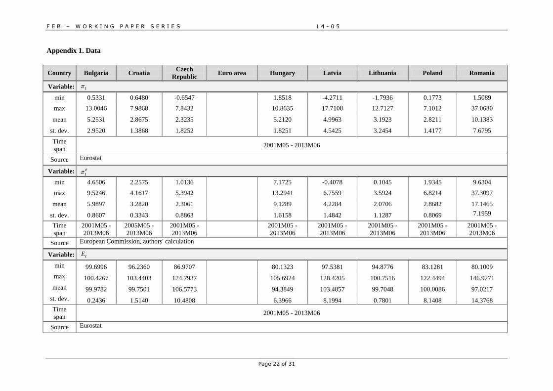
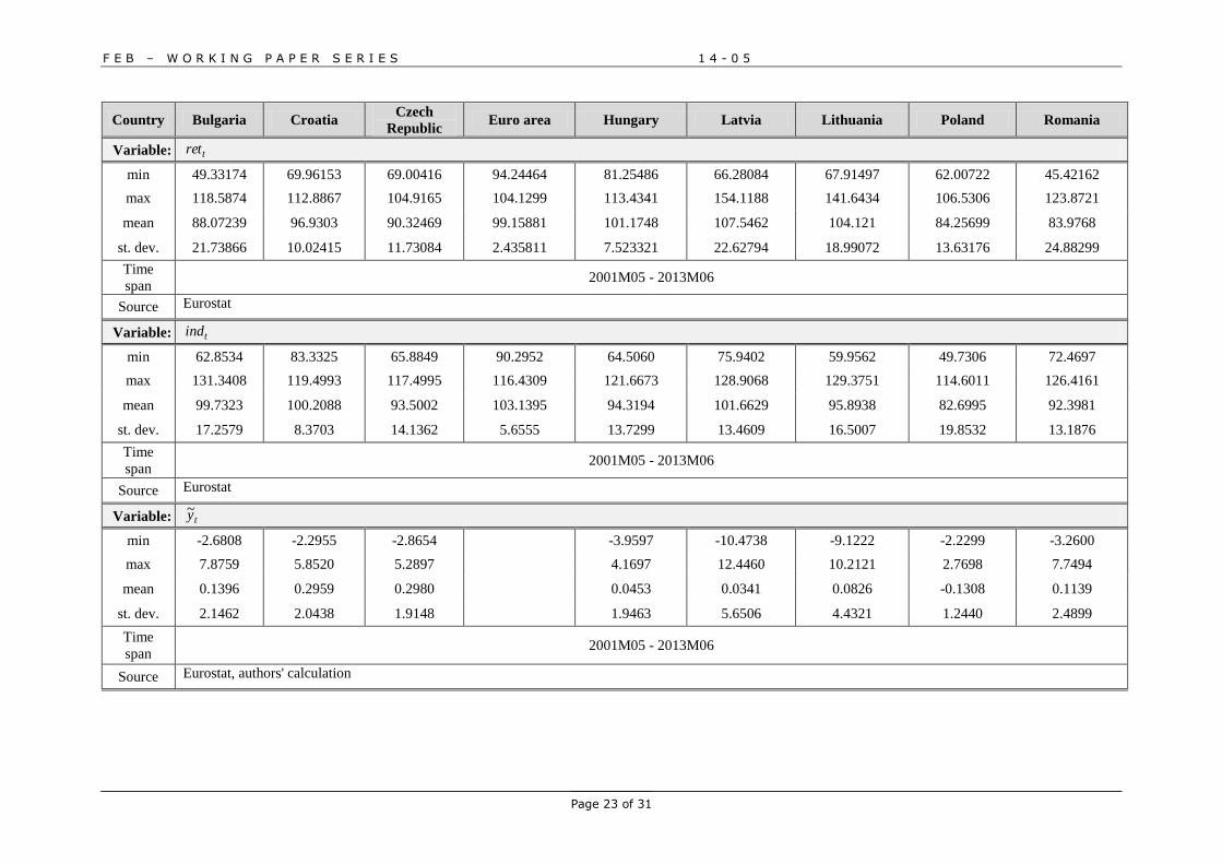
3.1. Data

The dataset analyzed in this paper comprises the following variables for each of the eight NMS: yearly

HICP inflation rate, t ; four domestic inflation determinants (output gap, ; inflation expectations

based on consumer surveys, , 1M monetary aggregate in natural logarithms, tM ; and the nominal

effective exchange rate (17 trading partners)4, ); and three external inflation determinants (the

eurozone output gap, ; crude oil spot price in dollars per barrel, ; and the eurozone 3-month

money market interest rate, *

ti ). All the observed variables are of monthly frequencies, spanning from

2001M05 to 2013M06, subject to data availability (for details see appendix 1). All variables are

seasonally adjusted using TRAMO/SEATS method. The data sources and descriptive statistics for all

the observed variables are also given in appendix 1.

3.1.1. Output gap calculation

Output gaps for both the eurozone and NMS have been calculated using GDP data. However, GDP for

all analyzed countries is available only on the quarterly basis. To deal with this issue, GDP data has

been interpolated, based on a state-space algorithm with the Kalman smoothing procedure. Industrial

production ( ind ) and retail ( ret ) have been used as regressors.

In order to calculate the output gaps, the Baxter-King (BK) filter (Baxter and King 1999) was

employed on the interpolated GDP.5 Therefore, in measuring the output gap, all fluctuations higher

than six and lower than 96 months were eliminated. The original BK filter has missing data at the

beginning and the end of the sample. To deal with this problem, the missing data was backcasted and

forecasted with an AR(12) model, as proposed by Stock and Watson (1999).

3 There is a voluminous body of literature on the P-star model. The reader may consult e.g. Belke and Polleit

(2006), Ozdemir and Saygili (2009) or Czudaj (2011) or for empirical verifications of the model. 4 Nominal effective exchange rate is obtained as a weighted geometric average of the bilateral exchange rates

against the currencies of 17 competing countries. 5 Besides the Baxter-King, the Hodrick-Prescott (HP) filter was also used for robustness check. However,

qualitatively, the results are very similar. The only difference is that the HP filter-based output gap is more

volatile, so results are not as smooth as with the BK filter. To conserve space, only the results estimated with the

BK filter are presented in the paper. However, the results with the HP filter are available upon request.


Page 8 of 31

3.1.2. Extracting inflation expectations

Consumer surveys (CS) represent qualitative examinations of consumers’ views on the relevant micro-

and macroeconomic variables. The CS question of particular interest here is the one targeting

consumers’ expectations regarding inflation dynamics in the following year.

Q6 By comparison with the past 12 months, how do you expect that consumer prices will develop in

the next 12 months? They will …

a) increase more rapidly, b) increase at the same rate, c) increase at a slower rate, d) stay about

the same, e) fall, f) don’t know.

Let a , b , c , d , and e be the fractions of respondents declaring that prices in the following year will

increase more rapidly, increase at the same rate, stay about the same, increase at a slower rate, and fall,

respectively. Having these data at hand, the researchers have several alternative routines for obtaining

numerical indicators of the expected inflation.

The most commonly used quantification method is established by Carlson and Parkin (CP) (1975),

who assume that a , b , c , d , and e can be represented by the corresponding areas under the

standardized normal density curve. Another viable route would be to employ the Pesaran (1987) and

Smith and McAleer (1995) approach, which does not model expected inflation as a function of

consumers’ subjective probability distribution. On the contrary, it sees inflation expectations as a

function of a specific nonlinear regression model. Nardo (2003) highlights several major pitfalls of

both mentioned procedures, so this paper chooses a less restrictive route and follows an approach

introduced by Theil (1952) and Batchelor (1986). They extract the difference between the fraction of

consumers who expect growing prices ( tttt cbaU ) and the percentage of those anticipating a

price decline ( tt eD ). Batchelor (1986) additionally scales the stated difference in order to obtain

inflation expectations.

tttt DUE 12 , (2)

where is the scaling factor obtained by assuming the long-term unbiasedness of expectations.

t

t

t

ttE 12 , (3)

where tπ is the actual inflation rate in time t . Thus the final expression for the economy-wide

inflation expectations is given by:

tt

t

tt

t

t

tt DUDU

E

12 . (4)

Since CS questions are conceptualized to reflect consumers’ economic attitudes at the 12 months' time

horizon (see Q6), tπ is also analyzed as the year-on-year rate of change.

3.2. Methodology

In order to measure the importance of foreign and domestic shocks to inflation, a structural vector

autoregression (SVAR) model with long run restrictions was applied. Firstly, the following reduced

VAR model was estimated:


Page 9 of 31

∑

(5)

where is a vector of constants, are the estimated matrices of coefficients, is a

vector of error terms, and is a vector of variables, which in this specific case comprises the

following variables in this order:

(6)

where are oil prices, is the eurozone output gap,

is the eurozone interest rate, is the

domestic output gap, is the nominal effective exchange rate, is the M1 monetary aggregate,

is the survey-based expected inflation and is the actual inflation. The justification for all the

included variables is given in section 2. The SVAR model was estimated using long run restrictions

such as in Blanchard and Quah (1989). However, most authors define only aggregate shocks in small

scale SVAR models with two or three variables (Blanchard and Quah 1989, Clarida and Galí 1994,

Galí 1999). Contrary to this approach, De Vita and Kyaw (2008) and Ying and Kim (2001) use larger

VAR systems to identify foreign and domestic determinants of capital flows. Building on these

assumptions, one can represent inflation as a function of a larger number of shocks, which can be

written as:

(7)

where the first three variables represent the foreign supply, demand and monetary shock, respectively.

The last variable is a composite domestic shock represented by . The structural shocks are

unobservable, so additional identifying assumptions are needed to uncover structural shocks from the

data. Equation (8) presents the SVAR model in the matrix form along with the imposed long run

restrictions to identify foreign and domestic shocks:

[

]

[ ]

[

]

(8)

Three foreign shocks in the model (supply, demand and monetary shock) are identified using the

following assumptions:

1. Oil prices are determined by the supply and demand on the world market. Therefore, they are

exogenous to both eurozone shocks (output gap and interest rate), as well as to all domestic shocks in

the long run. Thus, . This restriction identifies the supply shock.

2. Foreign variables are unaffected by domestic shocks in the long run, which is a valid

assumption in the case of small open economies. This assumption implies that , for . This restriction separates foreign from domestic shocks.

3. Real variables are unaffected by monetary shocks in the long run. This means that the

eurozone output gap does not react to a shock in the eurozone nominal interest rate in the long run,

thus . This restriction identifies the foreign demand and monetary shock.

4. Since foreign shocks are well identified, all other shocks are domestic. Five remaining

domestic shocks

are not individually identified, but they comprise the composite


Page 10 of 31

domestic shock which is a sum of all five remaining shocks. Restrictions on the domestic shocks are

placed in the form of a lower triangular matrix in order to obtain a just identified system. Examples for

this approach can be found in the literature, e.g. Galí (1999) or Francis and Ramey (2005).6

Given that the foreign shocks have been identified, while the domestic shocks have not, the analysis is

conducted on composite foreign and domestic shocks. Specifically, inflation can be written as a sum

of all eight shocks:

(9)

The composite foreign shock contains the foreign supply, demand and monetary shock, while the

composite domestic shock contains five remaining unidentified shocks. Inflation can therefore be

written as:

(10)

where

, and

.

Two separate models have been estimated for each analyzed country: DVAR as the benchmark model

and LVAR for the purpose of robustness check. In the DVAR models all I(1) variables were

differenced to satisfy the stationarity condition. Since macroeconomic time series in CEE countries of

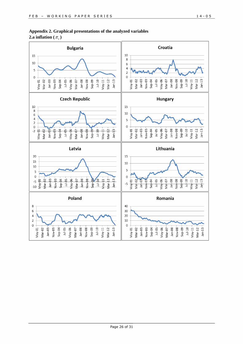
interest are rather volatile (see appendix 2 for graphical presentations of all the analyzed variables), it

is often very hard to detect the true order of integration. In order to tackle this issue, four different unit

root tests have been applied to determine the degree of integration of each variable: the Augmented

Dickey-Fuller (ADF) test, Kwiatkowski-Phillips-Schimdt-Shin (KPSS), Phillips-Perron (PP) test and

the Ng-Perron (NP) test. The obtained results are summarized in Table 1.

However, the LVAR models have been estimated with all the variables in levels. This model serves as

a robustness check and as an indicator of the DVAR’s appropriateness. The number of lags in each

VAR was chosen according to the Akaike information criterion.7

The importance of foreign and domestic shocks is analyzed by the forecast error variance

decomposition and historical decomposition of foreign and domestic shocks.8 Forecast error variance

decomposition shows the relative importance of each shock in the model. Historical decomposition

presents similar information, but in a different manner. It reveals the dynamics of inflation in absence

of all the shocks but one. Therefore, historical decomposition reproduces the time series of inflation,

which is only under the influence of foreign shocks, while the domestic ones are abstracted and vice

versa.

4. Results

The ADF test is conducted utilizing the Dolado, Jenkinson and Sosvilla-Rivero (1990) general-to-

specific approach, as well as the KPSS and Phillips-Perron tests. The results are summarized in Table

1. Since the obtained results obviously differ to some extent, the following estimation strategy was

pursued: a prevailing conclusion for each analyzed variable was drawn. E.g., if three out of four tests

indicated that the series is I(1), it was treated as such (i.e., it was differenced in the DVAR analysis). If

there was a tie (two I(0) vs. two I(1) decisions), the analyzed variable was also differenced in order not

to obtain spurious results.

6 In both papers authors estimate the augmented SVAR which only identifies a technology shock. All other

shocks are assumed to be non-technology shocks, which are not explicitly identified. 7 After estimating the reduced VAR, multivariate portmanteau (Q) autocorrelation test for 12 lags was applied.

In several cases, the number of lags in the VAR proposed by Akaike information criterion was insufficient to

resolve the autocorrelation issues. In those cases one additional lag was included in the model, which completely

resolved the autocorrelation problems. 8 Since the direction of the relationship between variables is not of a primary interest for this study, the impulse

response functions are not reported, but are available upon request.


Page 11 of 31

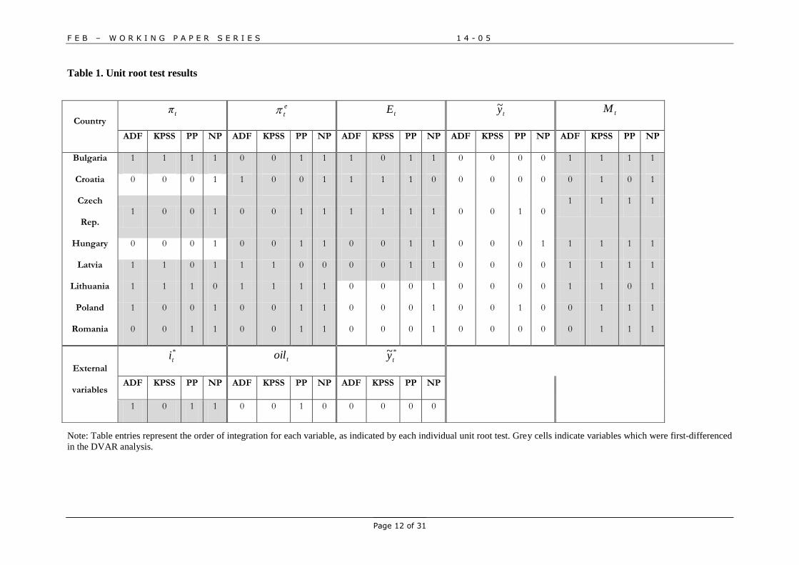
A glimpse at Table 1 reveals that e

t and tM can be treated as nonstationary for all observed

countries, while ty~ is uniformly stationary. The remaining variables exhibit rather mixed trending

properties. In some countries they are 0I , while in some they are 1I .9 The analysis is continued

through a structural DVAR model, where all the 1I time series are first-differenced.

4.1. Benchmark model

Figure 1 displays the forecast error variance decomposition of inflation in eight non-eurozone NMS in

order to measure the relative importance of two respective components (DOMESTIC and FOREIGN)

in determining the inflation variance.10

9 All the analyzed variables are stationary in first differences. The obtained unit root test results for differenced

data are left out here for brevity purposes but can easily be obtained from the authors upon request. 10

The period of analysis for every individual conutry corresponds to the data availability of monetary aggregate

M1 (given in Appendix 2).


Page 12 of 31

Table 1. Unit root test results

Note: Table entries represent the order of integration for each variable, as indicated by each individual unit root test. Grey cells indicate variables which were first-differenced

in the DVAR analysis.

Country tπ

e

t tE ty~ tM

ADF KPSS PP NP ADF KPSS PP NP ADF KPSS PP NP ADF KPSS PP NP ADF KPSS PP NP

Bulgaria 1 1 1 1 0 0 1 1 1 0 1 1 0 0 0 0 1 1 1 1

Croatia 0 0 0 1 1 0 0 1 1 1 1 0 0 0 0 0 0 1 0 1

Czech

Rep. 1 0 0 1 0 0 1 1 1 1 1 1 0 0 1 0

1 1 1 1

Hungary 0 0 0 1 0 0 1 1 0 0 1 1 0 0 0 1 1 1 1 1

Latvia 1 1 0 1 1 1 0 0 0 0 1 1 0 0 0 0 1 1 1 1

Lithuania 1 1 1 0 1 1 1 1 0 0 0 1 0 0 0 0 1 1 0 1

Poland 1 0 0 1 0 0 1 1 0 0 0 1 0 0 1 0 0 1 1 1

Romania 0 0 1 1 0 0 1 1 0 0 0 1 0 0 0 0 0 1 1 1

External

variables

*

ti toil *~ty

ADF KPSS PP NP ADF KPSS PP NP ADF KPSS PP NP

1 0 1 1 0 0 1 0 0 0 0 0


Page 13 of 31

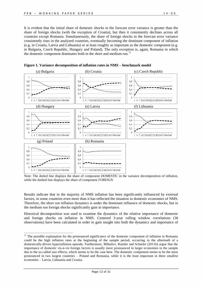
It is evident that the initial share of domestic shocks in the forecast error variance is greater than the

share of foreign shocks (with the exception of Croatia), but then it consistently declines across all

countries except Romania. Simultaneously, the share of foreign shocks in the forecast error variance

consistently rises in the analyzed countries, eventually becoming the dominant component of inflation

(e.g. in Croatia, Latvia and Lithuania) or at least roughly as important as the domestic component (e.g.

in Bulgaria, Czech Republic, Hungary and Poland). The only exception is, again, Romania in which

the domestic component dominates both in the short and medium run.11

Figure 1. Variance decomposition of inflation rates in NMS – benchmark model

(a) Bulgaria (b) Croatia (c) Czech Republic

(d) Hungary (e) Latvia (f) Lithuania

(g) Poland (h) Romania

Note: The dotted line displays the share of component DOMESTIC in the variance decomposition of inflation,

while the dashed line displays the share of component FOREIGN.

Results indicate that in the majority of NMS inflation has been significantly influenced by external

factors, in some countries even more than it has reflected the situation in domestic economies of NMS.

Therefore, the short run inflation dynamics is under the dominant influence of domestic shocks, but in

the medium run foreign shocks significantly gain in importance.

Historical decomposition was used to examine the dynamics of the relative importance of domestic

and foreign shocks on inflation in NMS. Centered 3-year rolling window correlations (36

observations) have been calculated in order to gain insight into both the dynamics and importance of

11

The possible explanation for the pronounced significance of the domestic component of inflation in Romania

could be the high inflation rates at the beginning of the sample period, occurring in the aftermath of a

domestically-driven hyperinflation episode. Furthermore, Mihailov, Rumler and Scharler (2011b) argue that the

importance of domestic vis-à-vis foreign factors is usually more pronounced in larger economies in the sample

due to the so-called size effects, which seems to be the case here. The domestic component seems to be the most

pronounced in two largest countries – Poland and Romania, while it is the least important in three smallest

economies – Latvia, Lithuania and Croatia.


Page 14 of 31

domestic and foreign components of inflation. It has been calculated for FOREIGN and t , as well as

for DOMESTIC and t .

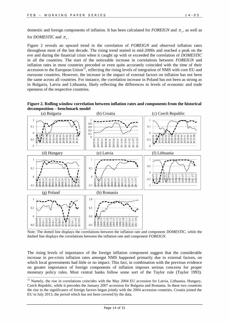
Figure 2 reveals an upward trend in the correlation of FOREIGN and observed inflation rates

throughout most of the last decade. The rising trend started in mid-2000s and reached a peak on the

eve and during the financial crisis when it caught up with or exceeded the correlation of DOMESTIC

in all the countries. The start of the noticeable increase in correlations between FOREIGN and

inflation rates in most countries preceded or even quite accurately coincided with the time of their

accession to the European Union12

, reflecting the rising levels of integration of NMS with core EU and

eurozone countries. However, the increase in the impact of external factors on inflation has not been

the same across all countries. For instance, the correlation increase in Poland has not been as strong as

in Bulgaria, Latvia and Lithuania, likely reflecting the differences in levels of economic and trade

openness of the respective countries.

Figure 2. Rolling window correlation between inflation rates and components from the historical

decomposition – benchmark model




Note: The dotted line displays the correlations between the inflation rate and component DOMESTIC, while the

dashed line displays the correlations between the inflation rate and component FOREIGN.

The rising levels of importance of the foreign inflation component suggest that the considerable

increase in pre-crisis inflation rates amongst NMS happened primarily due to external factors, on

which local governments had little or no impact. This fact, in combination with the previous evidence

on greater importance of foreign components of inflation imposes serious concerns for proper

monetary policy rules. Most central banks follow some sort of the Taylor rule (Taylor 1993). 12

Namely, the rise in correlations coincides with the May 2004 EU accession for Latvia, Lithuania, Hungary,

Czech Republic, while it precedes the January 2007 accession for Bulgaria and Romania. In these two countries

the rise in the significance of foreign factors began jointly with the 2004 accession countries. Croatia joined the

EU in July 2013, the period which has not been covered by the data.


Page 15 of 31

Typically, the Taylor rule sets the optimal interest rate as a function of inflation, real interest rate and

the output gap. For example, Galí (2009) proposes the following Taylor rule for the open economy:

(11)

where is the equilibrium real interest rate, is domestic inflation and represents the output

gap. Following the Taylor rule, and are non-negative coefficients. Full stabilization of domestic

prices requires the following condition:

. (12)

However, this rule stabilizes domestic prices, such as the GDP deflator. For open economies, imported

prices are also important; therefore HICP would be a more reasonable policy target. The findings of

greater importance of foreign in comparison to domestic shocks suggest that in case of small open

economies the Taylor rule should be augmented by foreign determinants of domestic inflation. In the

model in this study, all the three foreign shocks (supply, demand and nominal) proved to be important

in explaining domestic inflation.

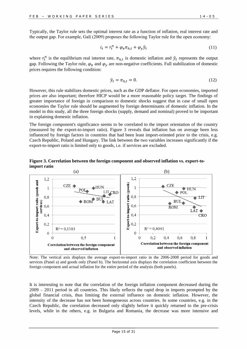
The foreign component's significance seems to be correlated to the import orientation of the country

(measured by the export-to-import ratio). Figure 3 reveals that inflation has on average been less

influenced by foreign factors in countries that had been least import-oriented prior to the crisis, e.g.

Czech Republic, Poland and Hungary. The link between the two variables increases significantly if the

export-to-import ratio is limited only to goods, i.e. if services are excluded.

Figure 3. Correlation between the foreign component and observed inflation vs. export-to-

import ratio

(a) (b)

Note: The vertical axis displays the average export-to-import ratio in the 2006-2008 period for goods and

services (Panel a) and goods only (Panel b). The horizontal axis displays the correlation coefficient between the

foreign component and actual inflation for the entire period of the analysis (both panels).

It is interesting to note that the correlation of the foreign inflation component decreased during the

2009 – 2011 period in all countries. This likely reflects the rapid drop in imports prompted by the

global financial crisis, thus limiting the external influence on domestic inflation. However, the

intensity of the decrease has not been homogeneous across countries. In some countries, e.g. in the

Czech Republic, the correlation decreased only slightly before it quickly returned to the pre-crisis

levels, while in the others, e.g. in Bulgaria and Romania, the decrease was more intensive and


Page 16 of 31

permanent.13

The behavior of inflation components could also be linked to domestic policy decisions.

For instance, in Poland, the decrease in the significance of the foreign component coincided with the

onset of the global financial crisis, to which the Polish authorities responded with a fiscal and

monetary expansion, accompanied by the 15 percent depreciation of the domestic currency (zloty).

This shifted the demand away from imports towards domestic products (Blanchard, Amighini and

Giavazzi 2010).

4.2. Robustness checks

In order to test the robustness of results obtained by the benchmark model, LVAR models have been

estimated. There is an obvious need for such robustness check for at least two reasons. First, the

results in the literature often differ depending on the use of DVAR or LVAR.14

However, Fernald

(2007) argues that both models should yield the same results. Opposite results occur in the presence of

structural breaks in the data, which generate false low frequency correlations. The second reason for

the use of LVAR is purely statistical. As was already mentioned, some variables in the DVAR model

were differenced although the unit root test results were not entirely conclusive.15

To check whether

this approach is reasonable, LVAR has been estimated. If both DVAR and LVAR yield similar results,

then the obtained inferences are robust across specifications, meaning that applying first differences in

several disputable cases was reasonable.

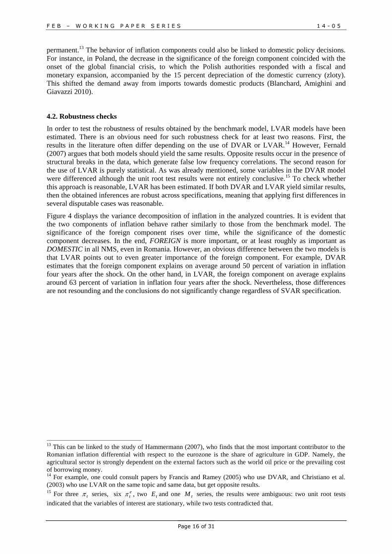
Figure 4 displays the variance decomposition of inflation in the analyzed countries. It is evident that

the two components of inflation behave rather similarly to those from the benchmark model. The

significance of the foreign component rises over time, while the significance of the domestic

component decreases. In the end, FOREIGN is more important, or at least roughly as important as

DOMESTIC in all NMS, even in Romania. However, an obvious difference between the two models is

that LVAR points out to even greater importance of the foreign component. For example, DVAR

estimates that the foreign component explains on average around 50 percent of variation in inflation

four years after the shock. On the other hand, in LVAR, the foreign component on average explains

around 63 percent of variation in inflation four years after the shock. Nevertheless, those differences

are not resounding and the conclusions do not significantly change regardless of SVAR specification.

13

This can be linked to the study of Hammermann (2007), who finds that the most important contributor to the

Romanian inflation differential with respect to the eurozone is the share of agriculture in GDP. Namely, the

agricultural sector is strongly dependent on the external factors such as the world oil price or the prevailing cost

of borrowing money. 14

For example, one could consult papers by Francis and Ramey (2005) who use DVAR, and Christiano et al.

(2003) who use LVAR on the same topic and same data, but get opposite results. 15

For three t series, six et , two tE and one tM series, the results were ambiguous: two unit root tests

indicated that the variables of interest are stationary, while two tests contradicted that.


Page 17 of 31

Figure 4. Variance decomposition of inflation rates in NMS – LVAR model




Note: The dotted line displays the share of component DOMESTIC in the variance decomposition of inflation,

while the dashed line displays the share of component FOREIGN.

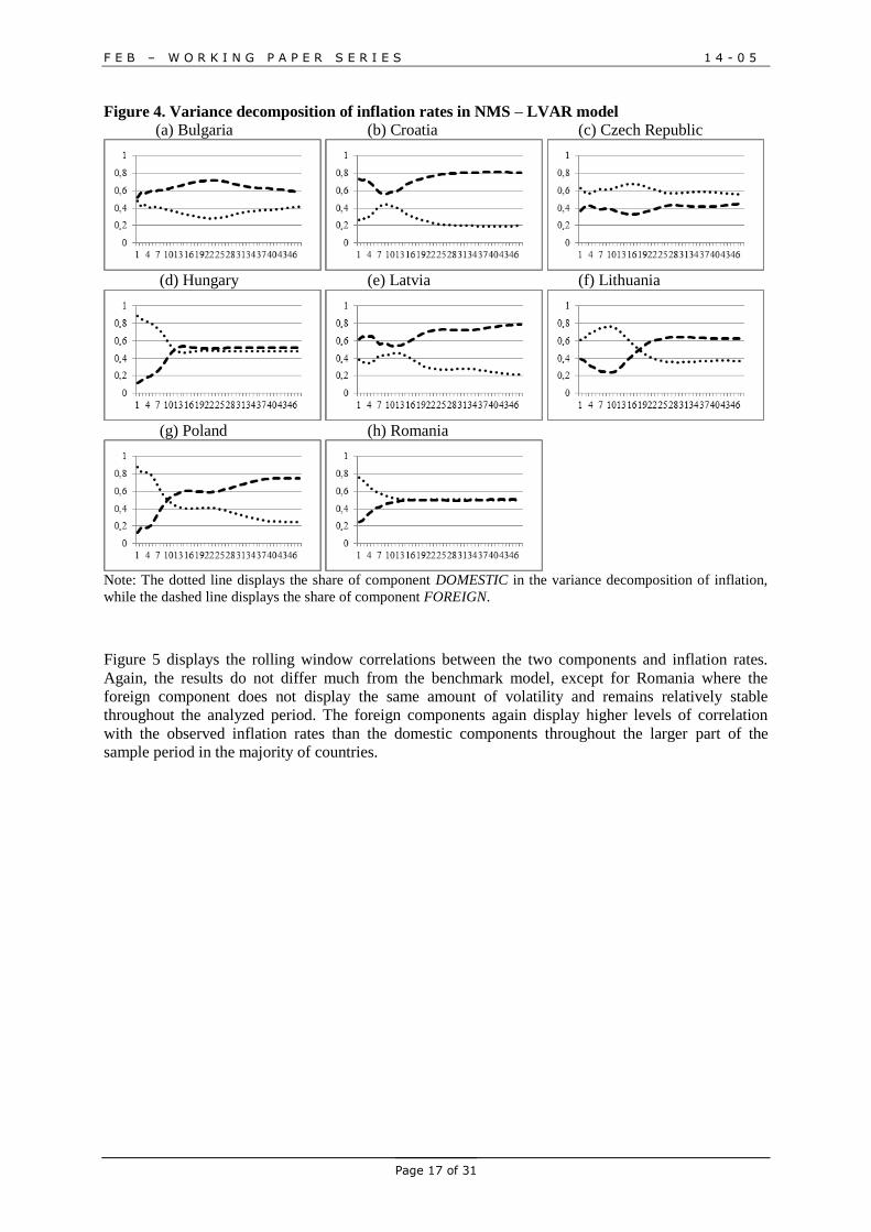
Figure 5 displays the rolling window correlations between the two components and inflation rates.

Again, the results do not differ much from the benchmark model, except for Romania where the

foreign component does not display the same amount of volatility and remains relatively stable

throughout the analyzed period. The foreign components again display higher levels of correlation

with the observed inflation rates than the domestic components throughout the larger part of the

sample period in the majority of countries.


Page 18 of 31

Figure 5. Rolling window correlation between inflation rates and components from the historical

decomposition – LVAR model




Note: The dotted line displays the correlations between the inflation rate and component DOMESTIC, while the

dashed line displays the correlations between the inflation rate and component FOREIGN.

5. Conclusion

This paper analyzed the importance of foreign and domestic determinants of inflation in case of the

New EU Member States. The empirical and theoretical approach taken in this paper is innovative in

several ways. First, it takes into account a much wider set of explanatory variables than the typical

new Keynesian Phillips curve framework. Second, inflation determinants are observed in a dynamic

SVAR framework. Finally, conclusions on the impact of structural changes such as the EU

enlargement and global financial crisis can be drawn using historical decomposition and rolling

window correlation.

The obtained results indicate that foreign shocks are either dominant or of similar importance as

domestic factors in explaining inflation dynamics in the medium run for the majority of the NMS. The

increasing importance of foreign shocks is clearly evident in all the NMS, and this conclusion is robust

across specifications. This means that, throughout the analyzed period, inflation in NMS has been

influenced severely by external factors, in some countries even more than by the situation in domestic

economies. However, the short run inflation dynamics is better explained by domestic factors.

The importance of foreign shocks started to increase in mid-2000s, which coincided with the time

when most of the analyzed countries joined the EU. On the other hand, the global financial crisis has

had an inverse impact. It caused a significant decline in importance of foreign shocks between 2009

and 2011 in most NMS. At the same time, domestic factors became more important in explaining

inflation. A possible explanation for this phenomenon is the relative openness of the analyzed

countries measured by their export to import ratio. More open countries experienced a rapid growth in


Page 19 of 31

the foreign component of inflation after their EU accession, while less open countries recorded a more

stable structure of both foreign and domestic components of inflation.

Finally, taking into account the fact that the foreign component proved to be very important in

explaining inflation, it could be concluded that the classical Taylor rule for conducting monetary

policy should be augmented by foreign determinants in case of small open economies, such as the

NMS.

Based on these conclusions, two promising areas of further research arise. The first one concerns

building an acceptable monetary policy rule for small open economies. As it is shown in this paper,

foreign driving factors of inflation should also be incorporated into such a policy rule. The second

fruitful area of research would be to extend the conclusions from this paper on measuring economic

costs of joining EMU in the case of the analyzed NMS. Namely, since foreign factors dominantly

drive domestic inflation, giving up monetary independence should not deviate much from the main

goal of central banks – price stability.


Page 20 of 31

References

Álvarez, L.J., Hurtado, S., Sánchez, I., and Thomas, C. 2011. “The impact of oil price changes on

Spanish and euro area consumer price inflation.” Economic Modelling 28, No. 1-2: 422-431.

Batchelor, R.A. 1986. “Quantitative v. qualitative measures of inflation expectations.” Oxford Bulletin

of Economics and Statistics No. 48: 99-120.

Baxter, M., and King, R. G. 1999. “Measuring business cycles: approximate band-pass filters for

economic time series.” Review of economics and statistics 81, No. 4: 575-593.

Belke, A., and Polleit, T. 2006. “Money and Swedish Inflation.” Journal of Policy Modeling 28, No.

8: 931-942.

Benkovskis, K. 2008. “The role of inflation expectations in the new EU member states: consumer

survey results.” The Czech journal of economics and finance 58, No.7-8: 298-317.

Blanchard, O., Amighini, A., and Giavazzi, F. 2010. “Macroeconomics: A European Perspective.” 1st

edition. Financial Times/ Prentice Hall.

Blanchard, O. and Quah, D. 1989. “The Dynamic Effects of Aggregate Demand and Supply

Disturbances.” American Economic Review 79, No. 4: 655-73.

Borio, C.E.V., and Filardo, A. 2007. “Globalization and inflation: new cross-country evidence on the

global determinants of domestic inflation.” BIS working papers 227, Bank for international

settlements.

Ca’ Zorzi. M.; Hahn, E.; and Sánchez, M. 2007. “Exchange Rate Pass-Through in Emerging

Markets.” The IUP Journal of Monetary Economics, IUP Publications 0, No.4: 84-102.

Calvo, G. 2001. “Capital market and the exchange rate: with special reference to the dollarization

debate in Latin America.” Journal of Money, Credit and Banking 33, No.2: 312-34.

Calza, A. 2009. “Globalization, domestic inflation and global output gaps: evidence from the euro

area.” International finance 12, No. 3: 301-320.

Carlson J.A., and Parkin M. 1975. “Inflation expectations.” Economica 42, No. 166: 123-138.

Chen, S.S. 2009. “Oil price pass-through into inflation.” Energy Economics 31, No. 1: 126-133.

Christiano, L.; Eichenbaum M.; and Vigfusson R. 2003. “What happens after a technology shock?”

NBER Working Paper no. 9819

Clarida, R., and Galí, J. 1994. “Sources of Real Exchange Rate Fluctuations: How Important are

Nominal Shocks?” NBER Working Paper No. 4658.

Czudaj, R. 2011. “P-star in Times of Crisis - Forecasting Inflation for the Euro Area.” Economic

Systems 35, No. 3: 390-407.

De Vita, G., and Kyaw, K. S. 2008. “Determinants of capital flows to developing countries: a

structural VAR analysis.” Journal of Economic Studies 35, No. 4: 304-322.

Dolado, J.; Jenkinson,T.; and Sosvilla-Rivero,S. 1990. "Cointegration and Unit Roots." Journal of

Economic Surveys 4, No. 3: 249-273.

Égert, B. 2011. "Catching-up and inflation in Europe: Balassa-Samuelson, Engel's Law and other

culprits." Economic Systems 35, No. 2: 208-229.

Fernald, J. G. 2007. “Trend breaks, long-run restrictions, and contractionary technology

improvements.” Journal of Monetary Economics 54, No. 8: 2467-2485.

Francis, N., and Ramey, V. A. 2005. “Is the technology-driven real business cycle hypothesis dead?

Shocks and aggregate fluctuations revisited.” Journal of Monetary Economics 52, No.8: 1379-

1399.

Franta, M.; Saxa, B.; and Šmídková, K. 2010. “The role of inflation persistence in the inflation

process in the new EU member states.” Czech journal of economics and finance 60, No. 6: 480-

500.

Galí, J. 1999. “Technology, employment, and the business cycle: Do technology shocks explain

aggregate fluctuations?” American Economic Review 89, No. 1: 249–271.

Galí, J. 2009. “Monetary Policy, inflation, and the Business Cycle: An introduction to the new

Keynesian Framework.” Princeton University Press.

Galí, J., and Gertler, M. 1999. “Inflation Dynamics: A structural Econometric analysis.” Journal of

Monetary Economics 44, No.2: 195-222.

Galí, J., and Monacelli, T. 2005. "Monetary Policy and Exchange Rate Volatility in a Small Open

Economy." Review of Economic Studies 72, No. 3: 707-734.

http://ideas.repec.org/a/icf/icfjmo/v05y2007i4p84-102.html

http://ideas.repec.org/a/icf/icfjmo/v05y2007i4p84-102.html


Page 21 of 31

Hallman, J.J.; Porter, R.D.; and Small, D.H. 1991. “Is the Price Level Tied to the M2 Monetary

Aggregate in the Long Run?” American Economic Review 81, No. 4: 841-858.

Hammermann, F., 2007. “Nonmonetary determinants of inflation in Romania: a decomposition.” Kiel

Working Paper No. 1322.

Hammermann, F., and Flanagan, M. 2009. “What explains inflation differentials across transition

economies?” Economics of Transition 17, No.2: 297–328.

Hodrick, R. J., and Prescott, E. C. 1997. “Postwar US business cycles: an empirical

investigation.” Journal of Money, credit, and Banking 19, No.1: 1-16.

Ihrig, J.; Kamin, S. B.; Lindner, D.; and Marquez, J. 2007. “Some Simple Tests of the Globalization

and Inflation Hypothesis.” International Finance Discussion Papers, Board of Governors of the

Federal Reserve System, No. 891.

Juselius, K. 1992. “Domestic and foreign effects on prices in an open economy: The case of

Denmark.” Journal of policy modelling 14, No. 4: 401-428.

Mihailov, A.; Rumler, F.; and Scharler, J. 2011a. “The Small Open-Economy New Keynesian Phillips

Curve: Empirical Evidence and Implied Inflation Dynamics.” Open Economies Review 22, No.2:

317-337.

Mihailov, A.; Rumler, F.; and Scharler, J. 2011b. “Inflation Dynamics in the New EU Member States:

How Relevant Are External Factors?” Review of International Economics 19, No. 1: 65-76.

Nardo, M. 2003. “The quantification of qualitative survey data: a critical assessment.” Journal of

Economic Surveys 17, No. 5: 645-668.

Ozdemir, K.A. and Saygili, M. 2009. “Monetary pressures and Inflation Dynamics in Turkey:

Evidence from P-Star Model.” Emerging Markets Finance and Trade 45, No.6: 69-86.

Pain, N.; Koske, I.; and Sollie, M. 2006. “Globalisation and Inflation in the OECD Economies.”

OECD Economics Department Working Papers, No. 524, OECD Publishing.

Pesaran, H. M. 1987. “The Limits to rational expectations.” Oxford. Basil Blackwell.

Petrović, P.; Mladenović, Z.; and Nojković, A. 2011. “Inflation triggers in Transition Economies:

Their Evolution and Specific Features.” Emerging Markets Finance and Trade 47, No. 5: 101-124.

Smith J. and Mcaleer M. 1995. “Alternative procedures for converting qualitative response data to

quantitative expectations: an application to Australian manufacturing.” Journal of Applied

Econometrics 10, No. 2: 165-185.

Stavrev, E. 2006. “Driving forces of inflation in the new EU8 countries.” Czech journal of economics

and finance 56, No. 5-6: 246-257.

Stock, J. H., and Watson, M. W. 1999. “Business cycle fluctuations in US macroeconomic time

series.” Handbook of macroeconomics, 1, 3-64.

Takhtamanova, Y.F. 2010. “Understanding changes in exchange rate pass-through.” Journal of

Macroeconomics 32, No. 4: 1118-1130.

Taylor, J. B. 1993. Discretion versus policy rules in practice. Carnegie-Rochester conference series on

public policy.” Vol. 39. North-Holland.

Theil H. 1952. “On the time shape of economic microvariables and the Munich business test.” Review

of the International Statistical Institute 20: 105-120.

Tica, J., and Posedel, P. 2009. “Threshold Model of the Exchange Rate Pass-Through Effect.“ Eastern

European Economics 47, No. 6: 43-59.

Vašíček, B. 2009. “Inflation dynamics and the new Keynesian Phillips curve in the EU-4.” William

Davidson Institute Working Paper, No. 971.

Vizek, M., and Broz, T. 2007. “Modeling inflation in Croatia.” Emerging markets finance and trade

45, No. 6: 87-98.

Ying, Y. H., and Kim, Y. 2001. “An empirical analysis on capital flows: the case of Korea and

Mexico.” Southern Economic Journal 67, No. 4: 954-968.


Page 22 of 31

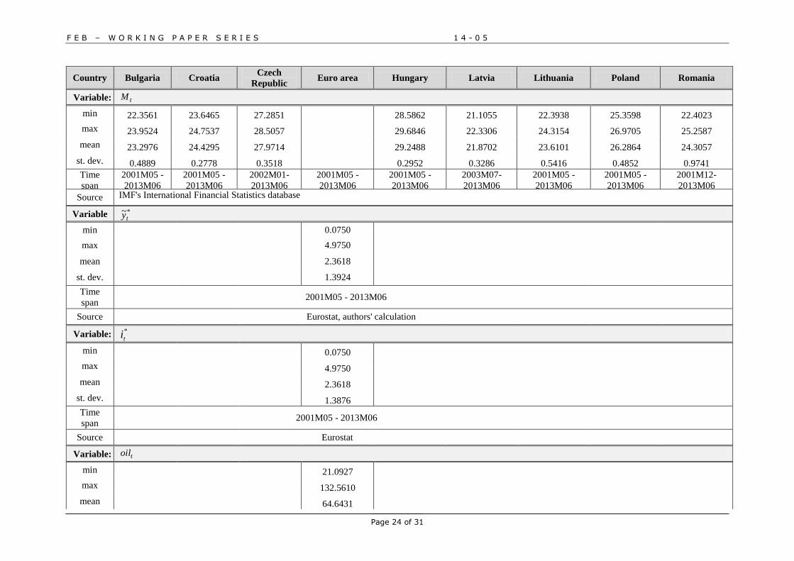
Appendix 1. Data

Country Bulgaria Croatia Czech

Republic Euro area Hungary Latvia Lithuania Poland Romania

Variable: t

min 0.5331 0.6480 -0.6547 1.8518 -4.2711 -1.7936 0.1773 1.5089

max 13.0046 7.9868 7.8432 10.8635 17.7108 12.7127 7.1012 37.0630

mean 5.2531 2.8675 2.3235 5.2120 4.9963 3.1923 2.8211 10.1383

st. dev. 2.9520 1.3868 1.8252 1.8251 4.5425 3.2454 1.4177 7.6795

Time

span 2001M05 - 2013M06

Source Eurostat

Variable: et

min 4.6506 2.2575 1.0136

7.1725 -0.4078 0.1045 1.9345 9.6304

max 9.5246 4.1617 5.3942 13.2941 6.7559 3.5924 6.8214 37.3097

mean 5.9897 3.2820 2.3061 9.1289 4.2284 2.0706 2.8682 17.1465

st. dev. 0.8607 0.3343 0.8863 1.6158 1.4842 1.1287 0.8069 7.1959

Time

span

2001M05 -

2013M06

2005M05 -

2013M06

2001M05 -

2013M06

2001M05 -

2013M06

2001M05 -

2013M06

2001M05 -

2013M06

2001M05 -

2013M06

2001M05 -

2013M06

Source European Commission, authors' calculation

Variable: tE

min 99.6996 96.2360 86.9707

80.1323 97.5381 94.8776 83.1281 80.1009

max 100.4267 103.4403 124.7937 105.6924 128.4205 100.7516 122.4494 146.9271

mean 99.9782 99.7501 106.5773 94.3849 103.4857 99.7048 100.0086 97.0217

st. dev. 0.2436 1.5140 10.4808 6.3966 8.1994 0.7801 8.1408 14.3768

Time

span 2001M05 - 2013M06

Source Eurostat


Page 23 of 31



Variable: tret

min 49.33174 69.96153 69.00416 94.24464 81.25486 66.28084 67.91497 62.00722 45.42162

max 118.5874 112.8867 104.9165 104.1299 113.4341 154.1188 141.6434 106.5306 123.8721

mean 88.07239 96.9303 90.32469 99.15881 101.1748 107.5462 104.121 84.25699 83.9768

st. dev. 21.73866 10.02415 11.73084 2.435811 7.523321 22.62794 18.99072 13.63176 24.88299

Time

span 2001M05 - 2013M06

Source Eurostat

Variable: tind

min 62.8534 83.3325 65.8849 90.2952 64.5060 75.9402 59.9562 49.7306 72.4697

max 131.3408 119.4993 117.4995 116.4309 121.6673 128.9068 129.3751 114.6011 126.4161

mean 99.7323 100.2088 93.5002 103.1395 94.3194 101.6629 95.8938 82.6995 92.3981

st. dev. 17.2579 8.3703 14.1362 5.6555 13.7299 13.4609 16.5007 19.8532 13.1876

Time

span 2001M05 - 2013M06

Source Eurostat

Variable: ty~

min -2.6808 -2.2955 -2.8654

-3.9597 -10.4738 -9.1222 -2.2299 -3.2600

max 7.8759 5.8520 5.2897

4.1697 12.4460 10.2121 2.7698 7.7494

mean 0.1396 0.2959 0.2980

0.0453 0.0341 0.0826 -0.1308 0.1139

st. dev. 2.1462 2.0438 1.9148

1.9463 5.6506 4.4321 1.2440 2.4899

Time

span 2001M05 - 2013M06

Source Eurostat, authors' calculation


Page 24 of 31



Variable: tM

min 22.3561 23.6465 27.2851

28.5862 21.1055 22.3938 25.3598 22.4023

max 23.9524 24.7537 28.5057 29.6846 22.3306 24.3154 26.9705 25.2587

mean 23.2976 24.4295 27.9714 29.2488 21.8702 23.6101 26.2864 24.3057

st. dev. 0.4889 0.2778 0.3518 0.2952 0.3286 0.5416 0.4852 0.9741

Time

span

2001M05 -

2013M06

2001M05 -

2013M06

2002M01-

2013M06

2001M05 -

2013M06

2001M05 -

2013M06

2003M07-

2013M06

2001M05 -

2013M06

2001M05 -

2013M06

2001M12-

2013M06

Source IMF's International Financial Statistics database

Variable *ty~

min

0.0750

max

4.9750

mean

2.3618

st. dev.

1.3924

Time

span 2001M05 - 2013M06

Source

Eurostat, authors' calculation

Variable: *

ti

min

0.0750

max

4.9750

mean

2.3618

st. dev.

1.3876

Time

span 2001M05 - 2013M06

Source

Eurostat

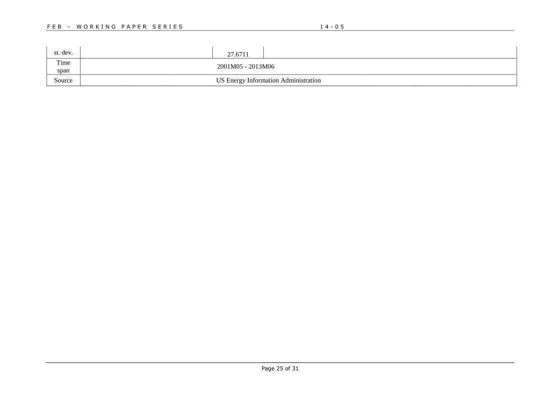
Variable: toil

min

21.0927

max

132.5610

mean

64.6431


Page 25 of 31

st. dev.

27.6711

Time

span 2001M05 - 2013M06

Source

US Energy Information Administration


Page 26 of 31

Appendix 2. Graphical presentations of the analyzed variables

2.a inflation ( t )


Page 27 of 31

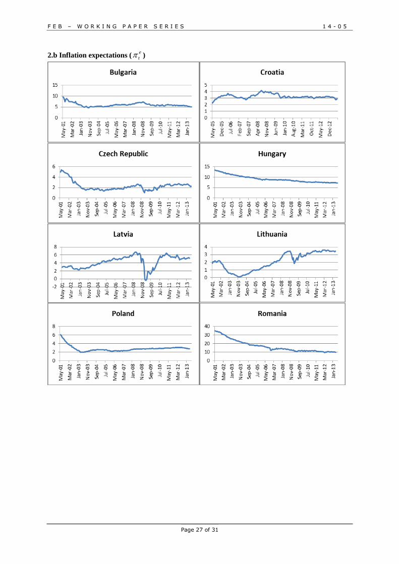
2.b Inflation expectations (e

t )


Page 28 of 31

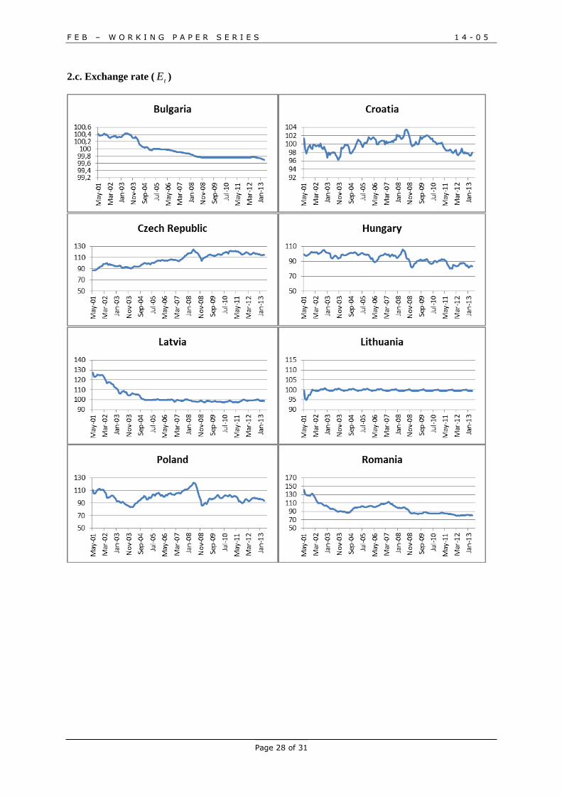
2.c. Exchange rate ( tE )


Page 29 of 31

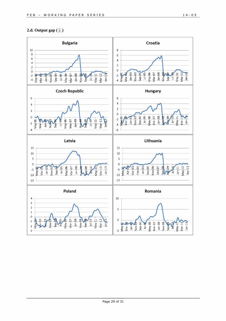
2.d. Output gap ( ty~ )


Page 30 of 31

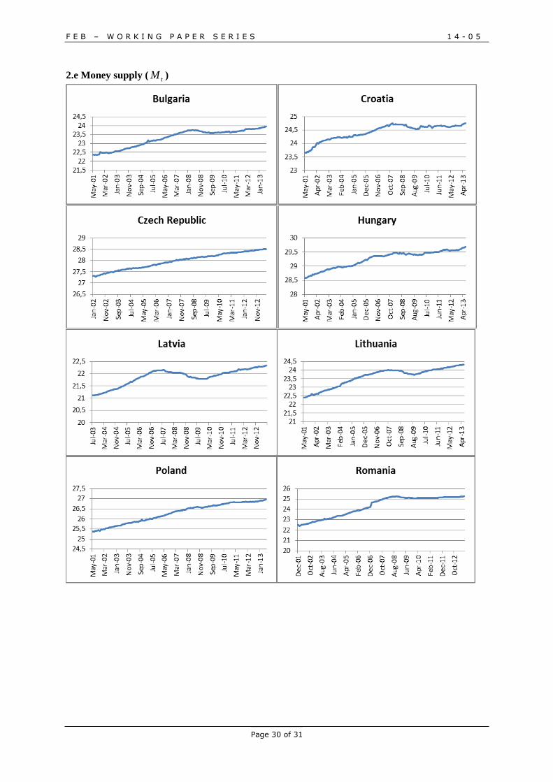
2.e Money supply ( tM )


Page 31 of 31

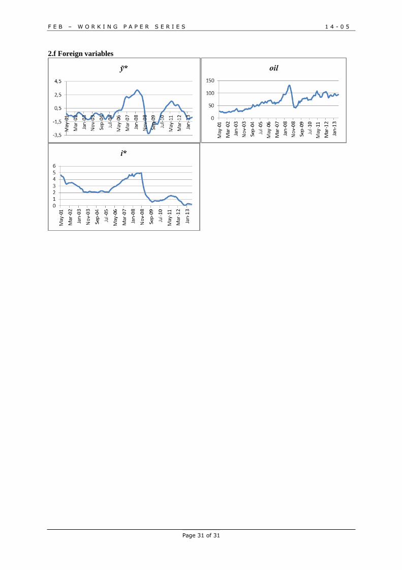
2.f Foreign variables

Documents

Tomislav Globan Vladimir Ar Petar Sorić Inflation in New EU …web.efzg.hr/repec/pdf/Clanak 14-05.pdf · · 2014-10-23importance of domestic vs. foreign inflation determinants