1

Being Surprised by the Unsurprising:

Earnings Seasonality and Stock Returns

Tom Y. Chang*, Samuel M. Hartzmark†, David H. Solomon* and Eugene F. Soltes‡

March 2015

Abstract: We present evidence consistent with markets failing to properly price information in

seasonal earnings patterns. Firms with historically larger earnings in one quarter of the year

(“positive seasonality quarters”) have higher returns when those earnings are usually announced.

Analysts have more positive forecast errors in positive seasonality quarters, consistent with the

returns being driven by mistaken earnings estimates. We show that investors appear to

overweight recent lower earnings following positive seasonality quarters, leading to pessimistic

forecasts in the subsequent positive seasonality quarter. The returns are not explained by a

number of risk-based explanations, firm-specific information, increased volume, or idiosyncratic

volatility.

*University of Southern California, †Chicago Booth School of Business ‡ Harvard Business School

Contact at tychang@marshall.usc.edu, samuel.hartzmark@chicagobooth.edu, dhsolomo@marshall.usc.edu and

esoltes@hbs.edu respectively. We would like to thank Joey Engelberg, Wayne Ferson, Dick Roll, Kelly Shue, Eric

So, Richard Thaler, and seminar participants at Arizona State University, DePaul University, the University of

Toronto, the USC Finance Brownbag, the NBER Behavioral Economics Meetings, Fuller and Thaler Asset

Management, the Southern California Finance Conference, and the USC/UCLA/UCI Finance Day.

2

1. Introduction

“Day-to-day fluctuations in the profits of existing investments, which are obviously of an

ephemeral and non-significant character, tend to have an altogether excessive, and even an

absurd, influence on the market. It is said, for example, that the shares of American companies

which manufacture ice tend to sell at a higher price in summer when their profits are seasonally

high than in winter when no one wants ice.” -John Maynard Keynes (1936)-

Many firms have predictably greater earnings at some points in the year than others,

usually due to the underlying cyclical nature of the firm’s business. To avoid misidentifying

seasonal patterns as genuine earnings news, the accounting literature has long examined

seasonally-adjusted earnings, often by methods like subtracting off same-quarter earnings from

prior years (e.g. Bernard and Thomas (1990) among others). Despite much attention on

identifying seasonal earnings, relatively less consideration has been given to how earnings

seasonality itself is priced. One likely reason for this divergence is that correcting for seasonal

patterns seems fairly straightforward. The fact that ice cream producers generate more earnings

in summer and snow-blower shops generate more earnings in winter would strike most people as

obvious to the point of being trite. Earnings seasonality thus seems to be tailor-made as an

example of an event whose reliability means that it is not news that should move prices in the

sense of Samuelson (1965).

Nevertheless, there is a growing body of evidence that many similarly obvious repeating

firm events are associated with puzzling abnormal returns. Abnormal returns are evident in

months forecasted to have earnings announcements, dividends, stock splits, stock dividends,

special dividends, and increases in dividends.1 Given these results, a natural question that arises

is what sorts of information are investors good at incorporating into prices. A standard

1 The returns in expected earnings announcement months are explored in Beaver (1968), Frazzini and Lamont

(2006), Savor and Wilson (2011), and Barber, George, Lehavy and Trueman (2013). Hartzmark and Solomon

(2013) document high returns in months with an expected dividend. Bessembinder and Zhang (2014) document high

returns in months predicted to have stock splits, stock dividends, special dividends, and increases in dividends.

3

information acquisition view posits that investors should have no issues measuring earnings

seasonality as it is both easy to interpret and repeated frequently for each firm in a timely

manner, thereby allowing ample opportunities for learning. However, from a behavioral

perspective the apparent simplicity of seasonal adjustments can be deceptive: while identifying

seasonal quarters may be easy, correcting for this variation can be considerably more difficult.

Repeated events that may appear to be well-understood are often less likely to attract the careful

attention of investors. Consequently, investors are prone to display biases when making

decisions related to such events.

In this paper, we present evidence of abnormal returns consistent with markets failing to

properly price information contained in seasonal patterns of earnings. Some companies have

earnings that are consistently higher in one quarter of the year relative to others, which we call a

positive seasonality quarter. We find that companies earn significant abnormal returns in months

when they are likely to announce earnings from a positive seasonality quarter.

Consider the example of Borders Books, which traded from 1995 to 2010. Borders Books

had a highly seasonal business, with a large fraction of earnings in the 4th

quarter, partly as a

result of Christmas sales. Out of Borders’ 63 quarterly earnings announcements, the 14 largest

were all 4th

quarter earnings. Not only did these quarters have high levels of earnings, but they

also had high earnings announcement returns – the average monthly market-adjusted return for

Borders’ 4th

quarter announcements was 2.27%, compared with -3.40% for all other quarters.

Earnings seasonality is a persistent property of the firm’s business, and thus an investor could

easily forecast when these high returns would occur. We show that the pattern in earnings

announcements returns for Borders holds in general for seasonal firms – high earnings

announcement returns can be forecast using past information about seasonal patterns in earnings.

4

To measure earnings seasonality, we rank a company’s quarterly earnings

announcements over a five year period beginning one year before portfolio formation. We then

calculate the average rank in the previous five years of the upcoming quarter. The highest

possible seasonality in quarter three, for instance, would be a company where the previous five

announcements in quarter three were the largest out of the 20 announcements considered.

A portfolio of companies with expected earnings announcements in the highest quintile

of earnings seasonality earns abnormal returns of 65 basis points per month relative to a four

factor model, compared with abnormal returns of 31 basis points per month for the lowest

seasonality quintile. This difference is statistically significant at the 1% level, and unlike many

anomalies it becomes stronger when the portfolio is value weighted (abnormal returns of 55 basis

points for the difference portfolio, with a t-statistic of 3.14). As the base returns in expected

earnings announcement months are generally positive due to the earnings announcement

premium (Frazzini and Lamont (2006)), another way of interpreting this finding is that the

earnings announcement premium is larger in months when earnings are expected to be higher.

The nature of the earnings seasonality measure makes it unlikely that these returns are

driven by seasonal firms having different fixed loadings on risk factors. In the first place, the

portfolio of highly seasonal firms does not show higher volatility than the portfolio of negative

seasonal firms. If earnings are higher than average in one month then they will be lower than

average in other months of the year, so firms tend to cycle through both the long and short sides

of the portfolio. To emphasize this point, we redo the analysis sorting only on whichever of the

firm’s four announcements had the highest and lowest seasonality, regardless of level (ensuring

we are only sorting on time-series variation within each firm) and the results are very similar. In

order for risk to explain the results, it must be that firms are more risky in months of positive

5

seasonality than other months. It is also worth noting that the risk cannot simply be coming from

increased exposure to the standard four factors, as the regressions already control for this.

We examine a number of alternative risk-based explanations, and fail to find support for

them. Savor and Wilson (2011) argue that the earnings announcement premium is driven by a

common earnings announcement risk factor. We show that the seasonality effect is not driven by

positive seasonality quarters having a greater exposure to a common source of earnings

announcement risk – when we include a portfolio of all firms with an earnings announcement,

exposure to this factor does not drive the results.

We also provide positive evidence of investor mistakes by examining analyst forecast

errors. If seasonality returns were only driven by risk, as in a discount rate explanation, it is not

clear why analyst forecast errors would be related to firm seasonality, thus the forecasts should

only relate to cash flows. Instead, we find that analyst forecast errors are more positive in

positive seasonality quarters. For firms that shift between high and low quintiles of seasonality,

the median forecast error in positive seasonal quarters is 7% of the overall shift in earnings

between high and negative seasonal quarters. Thus analysts on average correctly forecast 93% of

the seasonal shift in earnings, suggesting that they are underreacting to seasonality, not ignoring

it altogether. To the extent that individual investors may either make the same mistakes as

analysts, or may simply take analysts’ mistaken forecasts at face value, the portfolio returns are

consistent with mispricing rather than risk.

When we examine daily characteristic adjusted returns around earnings announcements,

we find that most of the abnormal returns occur in the short event window surrounding the

announcement. This pattern is consistent with investors and analysts being positively surprised

6

by the earnings news. This also suggests that the returns to seasonality are not driven by the same

factors that make earnings announcement returns high overall. The general returns to earnings

announcement months tend to accrue in the pre-announcement period, which Johnson and So

(2014) argue is driven by liquidity provision. Finally, we do not observe either a drift or a

reversal subsequent to the positive returns of the announcement, suggesting the price response is

capturing a permanent shift in returns due to information that was not incorporated in the price

prior to the announcement.

We hypothesize that the effects of seasonality are a result of investors incorrectly

processing patterns in data when forming estimates of future earnings. The availability heuristic

(Tversky and Kahneman (1973)) describes the theory that individuals estimate probabilities

according to the ease with which instances of an event can be brought to mind. As one example

of this, the recency effect describes how individuals are more likely to remember recent

information than old information (Murdock Jr (1962), Davelaar et al. (2005)). If an upcoming

quarter has positive seasonality, the level of earnings in the three most recent announcements

was likely lower than the announcement four quarters ago. If investors suffer from a recency

effect, they will be more likely to overweight recent lower earnings compared to the higher

earnings from the same quarter last year. This would cause them to be overly pessimistic about

the upcoming announcement, leading to greater positive surprises.

Consistent with a recency effect, we find that the seasonality effect is larger when

earnings in the three most recent announcements (typically 3, 6 and 9 months before portfolio

formation) were lower relative to earnings 12 months ago. This suggests that when the recent

news has been of a larger decrease in earnings relative to the positive seasonal quarter, investors

are more pessimistic when the positive seasonal quarter arrives. On the other hand, if there are

7

lower earnings before the seasonal quarter 12 months ago (typically 15, 18 and 21 months before

portfolio formation), this does not generate a spread in returns. This suggests that the recency of

low earnings is important in generating underreaction to seasonality. The seasonality effect is not

present when the firm has broken an earnings record in the past 12 months, an event which is

also likely to make the prospect of continuing good news salient to investors.

Earnings seasonality effects are not explained by other variables that have been

associated with the earnings announcement premium. Frazzini and Lamont (2006) argue that the

increase in turnover in earnings months drives the earnings announcement premium, and is

associated with increased investor attention. While positive seasonal months have more turnover

than negative seasonal months, there is no relationship between the increase in turnover and the

returns to seasonality, suggesting that the volume increase does not drive the returns. Barber,

George, Lehavy and Trueman (2013) show that earnings announcement returns are related to the

increase in idiosyncratic volatility. By contrast, returns to seasonality are similar between firms

with high and low expected idiosyncratic volatility, suggesting that the effects are distinct.

We also conduct a number of tests to show that seasonality is not simply proxying for

other time-series effects within the firm, including overall return seasonality (Heston and Sadka

(2008)), momentum, short-term reversals, or the dividend month premium (Hartzmark and

Solomon (2013)). The returns to seasonality also survive explicitly controlling for other

determinants of earnings changes, including past earnings surprises (Bernard and Thomas

(1990)), firm financial condition (Piotroski (2000)), and high accruals (Sloan (1996)). Earnings

seasonality is not some general driver of returns, as it does not forecast higher returns outside of

earnings months. The seasonality effect does not appear to be due to a tendency of firms to

engage in more earnings management in highly seasonal quarters. Seasonality is also unlikely to

8

be proxying for some recent information about the firm, however arising. Seasonality is highly

persistent across years, and lagging the measure by up to ten years produces similar results.

Overall, our results are consistent with investors not fully pricing in information

contained in earnings seasonality. The existence of abnormal returns around historically high

earnings levels points towards an emerging and puzzling stylized fact about asset returns, namely

that predictably recurring firm events tend to be associated with abnormal returns.

2. Related Literature

This paper contributes to several literatures in finance. Firstly, it is related to a number of

papers that document high returns during recurring and predictable time-series changes within

the firm. In addition to the reactions to firm-level events mentioned earlier, firms also have high

returns at increments of 12 months (Heston and Sadka (2008)). These findings about recurring

events are related to price responses to various one-off changes in prices and volumes, including

one month returns (Jegadeesh (1990)), 2 to 12 month returns (Jegadeesh and Titman (1993)), 3

to 5 year returns (DeBondt and Thaler (1985), and recent spikes in volume (Gervais, Kaniel and

Mingelgrin (2002)). We contribute to this literature by identifying a new anomaly based on

repeated and predictable variation in earnings levels.

Second, our paper also contributes to the literature examining underreaction and

information processing constraints. A number of papers have documented how prices can react

to information with a delay if investors have limited attention. Hirshleifer, Lim and Teoh (2009)

document that investors are more likely to underreact to earnings news on days with many

competing announcements, consistent with the announcements competing for limited total

investor attention. Da, Gurun and Warachka (2013) show that momentum in stock returns is

9

related to the tendency of investors to underreact to information that arrives in small increments.

Hirshleifer, Lim and Teoh (2011) argue that models of limited attention can explain post-

earnings announcement drift, the accrual anomaly, the profitability anomaly and the cash flow

anomaly. Our paper contributes to this literature by showing that an excessive focus on recent

events can cause investors to pay insufficient attention to longer term patterns in earnings, giving

another basis for information processing constraints.

Finally, this paper is related to the literature that examines how market participants form

estimates of firm earnings. A number of papers have explored how markets do not appear to

correctly forecast the autocorrelation of earnings news (Bernard and Thomas (1990), Ball and

Bartov (1995)). This finding is related to the apparent underreaction to earnings news, evidenced

by the post-earnings announcement drift (Ball and Brown (1968), Bernard and Thomas (1989,

1990), among others). Bernard and Thomas (1990) document that the underreaction to earnings

is significantly different at the 4th quarter horizon relative quarters 1 to 3. Johnston, Leone,

Ramnath and Yang (2012) provide evidence that markets and analysts fail to incorporate

predictable periodic changes in the length of firm fiscal quarters, another example of inattention

to recurring firm changes. So (2014) shows that firm revisions to earnings announcement dates

predict future news and returns. We extend this literature by directly evaluating the market’s

reaction to long-term patterns in earnings seasonality, and find evidence consistent with mistaken

estimates of the effect of seasonal patterns on current earnings.

Most related to the current work, Salomon and Stober (1994) examine the response to

earnings surprises depending on the seasonality of firm sales. They find evidence of higher

returns around high sales announcements after controlling for the level of the ex-post surprise,

and argue that this is due to resolution of uncertainty. We expand on this by examining the asset-

10

pricing implications of seasonality in a portfolio setting using only tradable ex-ante information

and controlling for known determinants of returns. We directly examine the role of idiosyncratic

risk and find it does not drive the returns, and instead we provide evidence of an alternative

explanation, namely biased cash-flow forecasts.

3. Analysis – Earnings Seasonality and Returns

3.1 Data

The data for earnings come from the Compustat Fundamentals Quarterly File. The data

on stock prices come from the Center for Research in Securities Prices (CRSP) monthly stock

file. Unless otherwise noted, in our return tests we consider stocks listed on the NYSE, AMEX

or NASDAQ exchanges, and consider only common stock (CRSP share codes 10 or 11). We also

exclude stocks that have a price less than $5 or a missing value of market capitalization at the

end of the previous month before returns are being measured. The data on analyst forecasts

come from the I/B/E/S detail file, and we consider forecasts of quarterly earnings per share. Data

on the excess market return, risk-free rate, SMB, HML and UMD portfolios come from Ken

French’s website.

3.2 Constructing measures of seasonality

To capture the level of earnings seasonality, we wish to measure the extent to which

earnings in a given quarter tend to be higher than other quarters. Conceptually, this includes both

a question of how often earnings are higher in a given quarter, and by how much they are higher

on average in a given quarter. The main measure we construct prioritizes the first component,

counting companies as having positive seasonality if they regularly have high earnings in a given

11

quarter. In the internet appendix we show the effect of measures using the size of the gap in

earnings across quarters, and find that both drive returns.

To construct our main measure of predicted seasonality in quarter t, we use 5 years of

earnings data from quarter t-23 to t-4. We compute firm earnings per share (excluding

extraordinary items) adjusted for stock splits.4 We then rank the 20 quarters of earnings data

from largest to smallest. We require non-missing values for all 20 quarters of earnings in order to

construct the measure. The main measure, earnrank, for quarter t is taken as the average rank of

quarters t-4, t-8, t-12, t-16, and t-20 – in other words, the average rank of same fiscal quarter

taken from previous years. A high value of earnrank means that historically the current quarter

of the year has larger earnings than other quarters, while a low rank of earnrank means that the

current quarter is low relative to other quarters. A firm whose earnings are randomly distributed

will tend to be in the middle of the distribution of earnrank.

While there are other ways one could measure seasonality, the current variable has

several advantages. Firstly, earnrank is not affected by the existence of negative earnings in

some periods, unlike measures that involve percentage changes in earnings. Second, it is

relatively invariant to the existence of large outliers in earnings numbers, such as from a single

very bad quarter. Third, by ranking earnings over several years, earnrank is less sensitive to

trends in overall earnings growth. If each quarter were only ranked relative to other quarters that

year, then companies with uniformly growing earnings would appear to have the maximum

possible seasonality in the 4th

quarter. By contrast, under the current measure, the rankings of the

4th

quarters would be 4, 8, 12, 16 and 20, giving an average rank of 12. This is considerably less

4 The main results of the paper are robust to alternative measures of earnings, such as total earnings, raw earnings

per share, earnings per share divided by assets per share, or earnings per share divided by share price.

12

than the maximum rank of 18, and empirically only 0.35 standard deviations above the median

value (11) and 0.45 standard deviations above the mean (10.85). In Table I Panel A, we present

summary statistics for the main variables used in the paper.

Given that firms either tend to cycle between extreme quintiles (if they have seasonal

shifts in earnings) or stay within the middle quintiles (if they have stable earnings over the

seasons), a question arises as to what type of firms have seasonal patterns in general. To examine

this, in Table II we take as the dependent variable the change in earnrank between a firm’s

highest and lowest announcement over the calendar year (for firms with 4 announcements). We

then examine how this varies with stock characteristics from the previous year – log market

capitalization and share turnover from the last month of the previous year, log book-to-market

ratio, accruals (Sloan 1996) and the log of firm age.

The results are presented in Table II. They indicate that seasonal shifts in earnings are

more common for large firms, value firms, old firms, low turnover firms, and firms with higher

accruals. All of these results are statistically significant at the 1% level when clustered by firm

and year (although market capitalization loses significance when date and industry fixed effects

are added). All these results are considerably reduced in magnitude when industry fixed effects

are added (using dummies for 48 industries from Fama and French (1997)), consistent with

industry factors being a significant driver of seasonal patterns in earnings. Because the main

examination of return differences is between firms in the extreme quintiles, the characteristics in

Table II do not obviously directly impact the returns to the portfolio, as general drivers of

seasonal shifts are likely to be common to both positive and negative seasonality firm/month

observations.

13

The requirement of 5 years of earnings data to form earnrank means that our sample will

be tilted somewhat towards older firms, though again this is true for both positive and negative

seasonality observations. It does however mean that the results may not generalize to young

firms who lack sufficient data to compute earnrank. Nonetheless, Table II implies that the

extreme quintiles are more likely to be filled with older firms, and hence the firms for which we

do not have earnrank data seem less likely to have large seasonal patterns anyway.

3.3 Seasonality and the Earnings Announcement Premium

We first examine whether information about earnings seasonality is incorporated into

stock prices. To do this, we examine stock returns in months when firms are predicted to have an

earnings announcement and sort based on the historical level of seasonality in earnings that

quarter. If the market has not fully incorporated the fact that earnings tend to be higher in certain

quarters, then the revelation of actual earnings will result in price movements. By contrast, if

markets are correctly forecasting the effect of seasonality, then the higher earnings in a given

quarter will not result in different stock returns.

Since the timing of an announcement may contain information, such as when a firm

delays an earnings announcement due to bad news (Frazzini and Lamont (2006)), we do not

condition ex-post on whether a firm has an earnings announcement in the month in question.

Instead, we predict whether a firm will have an earnings announcement in the current month,

based on whether or not it had an earnings announcement 12 months ago. The portfolio of all

stocks predicted to have an earnings announcement has abnormally positive returns, which is the

earnings announcement premium in Frazzini and Lamont (2006).

14

To examine the effects of earnings seasonality, we first condition on the existence of an

earnings announcement 12 months ago, and then sort firms into quintiles based on the level of

earnrank. As a result, all earnings information is a least 11 months old at the time of portfolio

formation. We form portfolios of returns for each quintile of earnrank, using breakpoints

calculated from the market distribution of earnrank in that month, with quintile 5 being firms

where earnings in the upcoming announcement were historically larger than other months. We

only include months where the portfolio has at least 10 firms, and in the case of the difference

portfolio, where both the long and short leg have at least 10 firms. It is worth emphasizing that

due to the earnings announcement premium all of the quintiles of earnrank are predicted to have

positive abnormal returns. The main question of interest then is whether seasonality causes larger

returns relative to other earnings announcements.

We consider this question in Table III Panel A. For the equal-weighted portfolio, the

highest seasonality quintile earns returns of 175 basis points per months, compared with 146

basis points per month for the lowest seasonality quintile. The gap is larger when value-

weighted portfolios are formed, with the positive seasonality quintile having returns of 176 basis

points per month, compared with 137 basis points per month for the lowest seasonality quintile.

Importantly, the positive seasonality portfolio is not more volatile. The negative

seasonality portfolio actually has the same or a slightly higher standard deviation of monthly

portfolio returns (5.28 equal weighted, 5.18 value weighted) than the positive seasonality

portfolio (5.14 equal weighted, 5.18 value weighted). This militates against some simple risk-

based explanations of the difference in portfolio returns, inasmuch as the higher returns to the

positive seasonality portfolio do not expose the investor to greater volatility. The various

snapshots of percentiles from the return distribution do not indicate that the positive seasonality

15

portfolio is more exposed to extreme negative returns, such as the crash risk associated with

momentum (Daniel and Moskowitz (2013)). The lowest monthly return is -18.0% for the equal-

weighted difference portfolio, and -14.9% for the value-weighted difference portfolio (compared

with maximums of 10.2% and 18.4% respectively).

In Table III Panel B, we examine the returns to seasonality in a panel setting. We again

sort firms into quintiles based on their level of earnrank for the upcoming announcement, and

then examine the average 3-day characteristic-adjusted return over the actual earnings

announcement date. The characteristic-adjusted returns are computed similar to Daniel,

Grinblatt, Titman and Wermers (1997) by subtracting off the returns of a value-weighted

portfolio matched on quintiles of market capitalization, ratio of book value of equity to market

value of equity (book to market ratio) and cumulative stock return from 12 months ago to 2

months ago (momentum). We compute this return not only for the upcoming announcement, but

for the subsequent four announcements. In each case, we compare whether the returns in quintile

5 are significantly different from those in quintile 1 by taking a sample of only those two

quintiles and regressing returns on a dummy variable for quintile 5, clustering by firm and date

(equivalent to a t-test but allowing for clustering).

The results confirm those of Panel A – firms in the positive seasonality quintile have

significantly higher returns than firms in the negative seasonality quintile. Consistent with firms

being likely to switch quintiles as seen in Table I, these returns have the opposite sign for the

following announcement. In addition, they retain the original sign and similar magnitude in four

quarters time, when the seasonality will be back to a similar level.

16

While Table III Panel A indicates that the positive seasonality portfolio does not have

higher volatility or skewness, these are not the only (or indeed the most important) measures of

risk. It may be that positive seasonality firm-months are exposed to other economy-wide risks

that investors care about. To test this, we examine the abnormal returns to earnings

announcement premium portfolios sorted on earnings seasonality, relative to a four factor model

controlling for excess market returns, size, book-to-market (Fama and French (1993)) and

momentum (Carhart (1997)). The returns of the earnings seasonality quintile portfolios are

regressed on the excess returns of the market, as well as the SMB, HML and UMD portfolios.

The results are presented in Table IV Panel A. This examines whether the returns to

portfolios formed on earnrank are explained by exposure to standard factors. For equal weighted

portfolios, the lowest seasonality quintile has a four factor alpha of 30.6 basis points per month

(with a t-statistic of 3.35), while the highest seasonality quintile portfolio has an alpha of 65.3

basis points per month (with a t-statistic of 6.98). The long-short portfolio has abnormal returns

of 34.7 basis points per month, with a t-statistic of 3.13. As in Panel A, the effects are stronger

when value weighted portfolios are used. The negative seasonality portfolio has abnormal returns

of 35.8 basis points (with a t-statistic of 2.77), while the positive seasonality portfolio has

abnormal returns of 90.9 basis points per month (with t-statistic of 6.03). The difference portfolio

has abnormal returns of 55.1 basis points per month, with a t-statistic of 3.14.

It is worth noting that the effect is driven by the long side of the portfolio. This is unusual

among anomalies, where a number of effects are concentrated in the short side (Stambaugh, Yu

and Yuan (2012)). Further, the largest distinction is between the highest seasonality quintile and

the remainder, with quintiles 1-4 showing similar abnormal returns to each other. The fact that

the majority of the anomaly comes from the firms with historically high earnings in the current

17

quarter is something we will return to when examining the possibility of investors being

pessimistic about the upcoming positive seasonality quarter due to a recency effect. The

abnormal returns are not monotonic across the quintiles, however. This may be due to the fact

that firms with little seasonal variation (those in the middle quintiles) tend to be younger and

smaller firms which have higher earnings announcement returns for other reasons. The main

variable of interest, however, is the difference between high and low levels of earnrank, which

will be less sensitive to firm characteristics. We return to this question shortly.

Secondly, the difference portfolios in Panel A have relatively low loadings on most of the

standard factors, having small and statistically insignificant loadings on excess market returns,

and UMD, and moderately but negative loadings on SMB and HML (meaning that the portfolio

tilts towards somewhat towards large growth firms).5 These low factor loadings arise because

firms with a seasonal pattern in earnings tend to cycle between the two extreme portfolios. For

instance, if a firm has unusually high earnings in the March quarter, it is more likely that it will

have unusually low earnings in some other quarter (relative to a firm with smooth earnings).

To emphasize this point, in Panel B we form portfolios that sort only on variation in

earnrank within the same firm over the course of a year. Specifically, for each firm that has four

values of earnrank in a given year, we compute where each earnrank value lies in the

distribution of firms that month. We then rank the firm’s four predicted earnings announcements

according to whichever had the highest, second highest, second lowest and lowest percentile

value of earnrank that year. Since all information in earnrank is at least 12 months old, this is

5 As a robustness check, we also compute the time series changes in factor loadings between positive seasonal

months using and surrounding earnings announcements using daily betas calculated as in Lewellen and Nagel

(2006). The changes in betas are generally negative and small in magnitude (between -0.080 and 0.006, depending

on the factor in question and the model). This supports the conclusion that positive seasonal months are not more

exposed to common factors known to explain returns.

18

computable by an investor before the start of the year over which returns are measured. The

resulting portfolios now include every firm in every portfolio once per year, and thus any

variation in seasonality is only coming from variation within the firm, rather than cross-sectional

variation from the types of firms that tend to have positive seasonality at some point in time.

Because the long and short portfolios cycle through the same set of firms, any fixed loadings on

factors will cancel out over time, and only time-varying exposure to factors will remain.

The results are shown in Table IV Panel B. The abnormal returns are similar to those in

Panel A – the equal-weighted difference portfolio has abnormal returns of 33.3 basis points (t-

statistic of 3.40) while the value-weighted difference portfolio has abnormal returns of 65.9 basis

points (t-statistic of 3.91). When within-firm variation is examined, the alphas are now

monotonic across the four announcements suggesting that the non-monotonicity in Panel B is

likely related to fixed firm characteristics.

The results in Panels A and B indicate that the abnormal returns are not driven by fixed

loadings on the market, SMB, HML or UMD. In addition, the abnormal returns cannot be

explained by positive seasonal months having consistently higher loadings on the factors being

controlled for (Mkt-Rf, SMB, HML and UMD). For instance, if firms always have a higher

market beta in positive seasonal months relative to negative seasonal months, then the difference

portfolio will buy firms in their high beta months and short them in their low beta months. As a

result, the difference portfolio will have a positive market beta, but the four-factor regression will

control for this, and hence it will not contribute towards the alpha.

More generally, because abnormal returns are evident using only within-firm variation,

the results are also not driven by fixed loadings on any other omitted factors, regardless of their

19

source. The results could however be driven by time-varying exposure to a risk source that we

are not measuring (e.g. something other than the market, SMB, HML and UMD), with firms

become riskier in positive seasonality months relative to negative seasonality months. We return

to this question in sections 4.1 and 4.4.

3.4 Effect of Earnings Seasonality versus other Seasonal Variables

While the previous table documents that seasonality is associated with abnormal returns

relative to a four-factor model, it is possible that by sorting on seasonality we are selecting for

some other anomaly that drives returns. Of particular concern are factors that involve predictable

changes in the firm over time. These include the dividend month premium (Hartzmark and

Solomon (2013)), where firms have abnormally high returns in months when they are predicted

to pay a dividend, and return seasonality (Heston and Sadka (2008)), where returns 12, 24, 36, 48

and 60 months ago positively predict returns in the current month. We also examine the effect of

other variables known to affect returns – log market capitalization, log book-to-market ratio,

momentum (returns from 12 months ago to 2 months ago) and last month’s return.

In addition, we wish to examine whether the effect of earnings seasonality is limited to

months with a predicted earnings announcement. If positive seasonality is associated with a

general period of increased exposure to economy-wide risks not specifically related to earnings,

then the higher returns may be evident in other months surrounding the positive seasonality

announcement.

We test these possibilities in Table V by examining the effect of earnings seasonality

using Fama Macbeth cross-sectional regressions – in each month, we run a cross-sectional

regression of stock returns on stock characteristics, then the time-series average and t-statistic

20

associated with each of the regression coefficients is computed. We consider two versions of the

regression. In columns 1-4, we consider only the cross-section of firms that had an earnings

announcement 12 months ago, and thus are predicted to have an earnings announcement in the

current month. The earnrank variable shows a significant predictive ability in a univariate

specification, with a coefficient of 0.034 and a t-statistic of 2.78. Since the standard deviation of

earnrank is 2.85, this means that a one standard deviation in seasonality corresponds to an

increase in returns during earnings months of 9.6 basis points. When additional controls are

included in column 2 for predicted dividends, Heston and Sadka (2008) seasonality, log market

cap, log book-to-market, momentum and one-month reversal, the coefficient is unchanged at

0.034 with a t-statistic of 2.95. The results are similar in columns 3 and 4 when the percentile

value of earnrank is used instead of the raw value.

In columns 4-8 we consider the cross-section of all firm-month observations, and include

a dummy variable for predicted earnings that we interact with the measure of seasonality. In this

specification, seasonality is matched to the predicted earnings month (i.e. 12 months after the

measure is formed) and the subsequent two months (13 and 14 months afterwards, respectively).

Column 5 is the all-firm equivalent of the univariate regression, including only seasonality, a

dummy for predicted earnings, and the interaction between the two. The regression shows that

only the interaction of predicted earnings and seasonality shows a significant positive effect, with

a coefficient of 0.051 and a t-statistic of 3.71. Earnings seasonality has a somewhat negative

effect in non-earnings months, although this effect becomes only marginally significant with the

inclusion of controls in column 5. The results are again similar if earnrank is measured as a

percentile. Seasonality does not seem to be proxying for other drivers of returns, nor does it

predict high returns outside of months with a predicted earnings announcement.

21

3.5 Earnings Seasonality and Delayed Reaction to Firm Specific Information

While the results in subsection 3.3 and 3.4 suggest that the seasonality effect is not

proxying for some fixed property of firms, it is possible that seasonality is correlated with other

recent firm-specific information that is announced in earnings months. This may relate to some

other property of earnings (such as earnings growth or post earnings announcement drift), or any

other number of changes in the firm. Earnrank is already constructed using 5 years of data and

then lagged one year before portfolios are formed, so by its nature it contains information from a

long time period, but it is still possible that information flows over this period drive the results.

Rather than trying to control for each possible type of firm-specific information, we test a

common prediction of such theories: namely, that firm-specific information should become less

relevant over time. As seasonality is a property of the firm’s underlying business model, it is

likely to be quite persistent over time. In addition, the timing of earnings announcements is

strongly persistent over time (Frazzini and Lamont (2006)), meaning that long-term earnings

information is still reasonably predictive of the timing of current announcements.

To test whether firm-specific information explains our results, we lag the earnrank

measure over different lengths of time. We show this in Table VI. In Panel A, we consider the

effects of seasonality from the same quarter of the year, but lagged in various multiples of 12

months when forming portfolios. This retains the prediction of seasonality for the current

quarter, but omits more and more of the recent earnings news of the firm. We examine lags of up

to ten years. While this restriction conditions on firms having a longer time series of data, the

resulting selection effect is equal between the long and short legs of the portfolio, so it should not

mechanically increase or decrease the returns to the difference portfolio.

22

The results show that statistically significant abnormal returns are evident even when

using information that is at least 10 years old (i.e. the earnrank measure is computed using

information from 10 years to 14 years before the portfolio formation date). The equal-weighted

difference portfolio has positive returns that are significant at a 5% level or more at every annual

horizon up to 10 years, while the value-weighted portfolio drops below the 5% level only at the

10 year mark. A curious aside is that the main effects actually get slightly larger when lagged

two and three years (54-55 basis points equal weighted, 64-68 basis points value-weighted). 6

In Panel B, we consider another prediction of delayed response to firm-specific earnings

information. In particular, if our results are driven by seasonality in earnings, then earnrank

should positively predict returns for the same quarter as the measure, but not have the same

results for other quarters. If positive seasonality effects were driven by a slow response to some

other correlated earnings news (such as earnings growth or post earnings announcement drift),

the effect should be similar when lagged at other multiples of 3 months, and indeed ought to be

stronger for horizons less than 12 months. When earnrank is lagged 3 months (i.e. using the

most recent earnings information), there is no spread in returns. At 6 months the returns are

similar when equal weighted but smaller and insignificant when value weighted. At 9 months,

the spread is significantly negative when value weighted, but not when equal weighted.

These results are difficult to reconcile with seasonality measuring some firm-specific

information flows that are common to recent earnings announcements – earnings information

6 The fact that the big increase comes from excluding earnings information from 12 to 23 months ago suggests that

earnings levels at this specific time may have contaminating factors. This is consistent with the fact that abnormally

high earnings from 4 quarters ago (roughly 12 months ago) tend to forecast low current month returns, as the post-

earnings announcement drift reverses at the 4th

quarter horizon (Bernard and Thomas (1990)).

23

shows persistent effects at long multiples of 12 months (consistent with a seasonality effect), but

generates weaker and different patterns at other horizons.

4. Explaining the Seasonality Effect – Risk versus Mistaken Earnings Forecasts

4.1 Earnings Announcement Risk and Analyst Forecast Errors

Perhaps the most standard potential explanation for the higher expected returns in

positive seasonality months is that they represent compensation for risk. While the regressions in

sub-sections 3.3 suggest that the patterns in returns are not driven by fixed factor loadings, the

announcements themselves may cause exposure to risks. Specifically, it is possible that

announcing a larger proportion of total annual earnings may make the stock more exposed to

announcement risk.

The most obvious way through which announcement risk could explain the results would

be if seasonality were associated with greater exposure to a systematic risk factor. This

systematic announcement risk must be separate from market returns during that month, as the

four factor regressions already control for different market betas across the long (positive

seasonal) and short (negative seasonal) portfolios. For idiosyncratic announcement risk to be

associated with higher returns, investors must be somehow prevented from diversifying this

idiosyncratic risk away by holding a portfolio of seasonal firms. This is assumed in Barber et al.

(2013) (who examine the relationship between idiosyncratic risk and earnings announcement

returns) and Johnson and So (2014) (who examine the returns to liquidity provision in the lead-

up to earnings announcements). In this view, the higher returns and lower volatility of the

portfolio of positive seasonal firms is not actually obtainable by the investor, as they can only

hold some subset of the firms (and thus face idiosyncratic risk). Whether or not investors are so

24

constrained is a separate question, and one beyond the scope of this paper. We return to the

question of whether idiosyncratic risk can explain the seasonality effect in section 5.1.

Table III Panel A indicates that the portfolio of highly seasonal firms does not have more

volatile returns than the portfolio of negative seasonal firms. While this does not conclusively

rule out a greater exposure to particular sources of risk, it does suggest that any systematic risk

exposure is being offset by lower risk exposure elsewhere such that the overall volatility is not

different.

Nonetheless, systematic risk factors related to earnings announcements are not

implausible. Savor and Wilson (2011) argue that there is a systematic component to earnings

announcement risk, and that the portfolio of firms with expected earnings announcements

represents a priced factor that proxies for the systematic component of earnings announcement

risk. If highly seasonal firms have more exposure to this overall earnings announcement risk

factor, this could be driving the pattern we document in returns.

We explore this possibility in Table VII. The regressions are similar to those in Table II,

taking portfolios of firms sorted on earnings rank, but in addition to the standard four factors

(excess market return, SMB, HML and UMD) we also include the excess returns of an equal-

weighted portfolio of all firms with a predicted earnings announcement that month (EARNRF).

This is designed to capture the overall fluctuation in returns for firms announcing earnings that

month, thereby proxying for the exposure to announcement risk.

The results indicate that exposure to an overall earnings risk factor does not drive the

seasonality effect. The difference in alphas (now a five-factor alpha, including exposure to the

overall earnings announcement factor) between positive and negative seasonality portfolios is

25

still large and significant: 34 basis points in Panel A when equal weighted (with a t-statistic of

3.00) and 48 basis points when value weighted in Panel B (with a t-statistic of 2.67). These

numbers are similar to those in Table IV (35 and 55 basis points respectively), indicating that

adding in an earnings risk factor does not explain the seasonality effect. This conclusion is

reinforced by the fact that the seasonality difference portfolio does not have any significant

loading on the earnings risk portfolio in either the equal-weighted or value-weighted tests. In

untabulated results, we show that different proxies for earnings risk (such as a value-weighted

portfolio of earnings announcement firms, or a difference portfolio between expected announcers

and non-announcers) produce similar spreads in abnormal returns.

More broadly, if seasonality returns are driven entirely by compensation for risk, then

market participants should not show a more positive average ex post surprise when cash flows

are announced. Earnings risk operates only through the discount rate channel – investors require

higher returns in positive seasonal months because of risk in these months, not because they are

more positively surprised on average by cash flows. In the case of earnings, we can test the latter

possibility quite cleanly because of the existence of analysts’ forecasts of earnings. Since these

are only forecasts of cash flows, the mean level of the surprise should not be affected by

seasonality under a risk-based explanation. There may be greater variability in forecast errors in

months where earnings are larger, but any increase in the mean level of forecast error is prima

facie evidence that analysts are relatively more pessimistic in months of positive seasonality.

In Table VIII we test whether analysts tend to be more positively surprised by firm

earnings in positive seasonality quarters. The unit of observation is at the firm-date level, and the

main dependent variable is the forecast error associated with the median quarterly earnings per

26

share forecast, taken over all analysts making forecasts between 3 and 90 days before the

earnings announcement.

The measure of forecast error is calculated as (Actual EPS – Forecast EPS) / Price (t-3).

In Panel A, we regress the panel of firm-date observations of earnrank and various controls. In

columns 1-4 we add controls for the log number of estimates being made, the standard deviation

of forecasts (divided by the price three days before the announcement, with the variable set to

zero if there is only one analyst), a dummy variable for cases whether there is only one analyst

making a forecast, the log market capitalization in the previous month, the log book to market

ratio, stock returns for the previous month, stock returns for the previous two to twelve months

cumulated, as well as the previous four forecast errors.

In the univariate specification in column 1, the coefficient on earnrank is 0.032, with a t-

statistic of 11.43 when clustered by firm and day. This shows that the earnings forecast error is

more positive when seasonality is high. In columns 2-4 we show that the effect of seasonality

survives the addition of firm-level controls, with a coefficient of 0.012 and a t-statistic of 5.19

when all firm controls are used. In column 5-7, we add date and firm fixed effects to control for

omitted variables related to overall firm differences and time-series changes in the overall

analyst mistakes. The effects are substantially similar, indicating that the effect of seasonality on

forecast errors is not simply due to the types of firms likely to be highly seasonal or the periods

of the sample when positive seasonality is more common. Table VIII is consistent with investors

and analysts being more positively surprised by firm cash flows during positive seasonality

quarters, and does not support explanations based on earnings risk.

27

To obtain a sense of the magnitude of these forecast errors, one can compare the forecast

error in positive seasonal quarters with the overall change in earnings between high and negative

seasonal quarters. This gives an estimate of the fraction of the overall change in earnings due to

seasonality that analysts are missing. To do this, we take firms that were in the highest quintile of

seasonality in the current quarter, and were also in the lowest quintile of seasonality at some

point in the past 12 months. For each of these firms, we compute the fraction of the seasonal shift

that was forecast as follows:

𝐹𝑟𝑎𝑐𝑡𝑖𝑜𝑛 𝐹𝑜𝑟𝑒𝑐𝑎𝑠𝑡

= [𝐻𝑖𝑔ℎ 𝑆𝑒𝑎𝑠𝑜𝑛𝑎𝑙𝑖𝑡𝑦 𝑀𝑒𝑑𝑖𝑎𝑛 𝐸𝑃𝑆 𝐹𝑜𝑟𝑒𝑐𝑎𝑠𝑡 − 𝐿𝑜𝑤 𝑆𝑒𝑎𝑠𝑜𝑛𝑎𝑙𝑖𝑡𝑦 𝐴𝑐𝑡𝑢𝑎𝑙 𝐸𝑃𝑆]

[𝐻𝑖𝑔ℎ 𝑆𝑒𝑎𝑠𝑜𝑛𝑎𝑙𝑖𝑡𝑦 𝐴𝑐𝑡𝑢𝑎𝑙 𝐸𝑃𝑆 − 𝐿𝑜𝑤 𝑆𝑒𝑎𝑠𝑜𝑛𝑎𝑙𝑖𝑡𝑦 𝐴𝑐𝑡𝑢𝑎𝑙 𝐸𝑃𝑆]

Among firms that shifted from the low quintile of seasonality to the high quintile of seasonality,

the median fraction forecast was 0.93, meaning that analysts correctly forecast 93% of the

seasonal shift in earnings but missed 7%. This reinforces the notion that the returns in positive

seasonal quarters are consistent with an underreaction to information in seasonality, but that this

does not imply that seasonality is ignored altogether.

In Panel B, we examine how analyst forecast errors vary over the subsequent four

quarters. Similar to Table III Panel B, we sort firms into quintiles and examine the difference

between the highest and lowest rank of earnrank. We again find that the difference between the

quintiles is highly significant in quarter t, and also in quarter t+4. Interesting, forecast errors are

also more positive in quarter t+3, a result for which we do not have a clear explanation.

4.2 Daily Returns

28

To further understand what is driving the returns that we observe in an earnings month,

we examine the daily returns surrounding earnings announcements. There are various

mechanisms surrounding earnings announcements that have been found to impact returns and

each of these suggest the returns will appear in different portions of the month. Barber et al.

(2013) and Johnson and So (2014) show that the earnings announcement premium is actually

concentrated prior to the earnings announcement itself. Thus if we are capturing a variant of this

effect we expect the returns to be concentrated several days before the announcement. The

returns at the monthly horizon may also be capturing effects after the initial announcement due

to post earnings announcement drift. To the extent that seasonality is proxying for a predictable

positive surprise, we expect to see returns concentrated at the announcement itself. While a

concentration of returns on the announcement day would also be consistent with a risk

explanation, the evidence in Section 3 suggests that this is not the driver of returns.

To test these predictions we examine characteristic-adjusted returns around earnings

announcements. Similar to Daniel, Grinblatt, Titman and Wermers (1997) we assign each stock

to a quintile based on size, book value, and momentum (using returns from t-20 to t-250). We

take the daily return for the stock and subtract the average return for the stocks in the market that

match these three quintiles. Where possible we use the filters from DellaVigna and Pollet (2009)

to identify the earnings announcement day.

Table IX presents the results and shows that returns are concentrated directly around the

earnings announcement itself. The first three columns show the average characteristic returns by

day for the highest quintile of seasonality, the lowest quintile and the middle three quintiles.

Similar to Barber et al. (2013) we find that the positive abnormal returns surrounding earnings

announcements in general begin several days before the earnings announcement itself. These

29

returns contain both the impact of the earnings announcement premium as well as that of

seasonality, so in order to see the impact of seasonality further tests are needed.

The fourth column in Table IX examines the difference in characteristic adjust return

from the top quintile and the bottom quintile of seasonality (similar to the portfolio sorts in Table

III). The largest return occurs on the announcement day itself, earning roughly 10 basis points

with a t-statistic of 3.37. Adding up the coefficients from t-2 to t+1 yields roughly 26 basis points

of returns. Comparing this to the equal weighted portfolio result of 35 basis points in Table III,

this suggests that most of the returns due to seasonality are related to the announcement itself.

The final column shows regression estimates of daily abnormal returns on earnings seasonality.

On each day surrounding an earnings announcement the characteristic-adjusted return is

regressed on earnrank. The coefficients that are both economically and statistically significant

are clustered around the announcement from t-2 to t+1. The largest effect occurs on the

announcement date itself and the second largest occurs on the day after the announcement. The

differential returns to seasonality are limited to a shorter period around the announcement,

consistent with a predictable positive surprise in earnings occurring in seasonal quarters.

4.2 Underreaction to Seasonality, the Recency Effect and Levels of Recent Earnings

The second broad class of explanation for seasonality affecting stock returns is that

markets are underweighting information contained in past seasonality information. If investors

do not fully account for the fact that earnings are predictably higher in certain quarters, then they

may be positively surprised when upcoming earnings are at high levels. The results in Table VIII

are consistent with analysts being more positively surprised in positive seasonal quarters.

Though this does not necessarily mean that other investors are also more surprised, it does

30

suggest the possibility of a common reaction of positive surprise by financial market participants

which may be driving the high returns.

As Ball and Bartov (1995) note, finding mistakes in investors’ reactions to particular

earnings announcements does not mean that investors are ignoring earnings news entirely. The

same is true of seasonality – we document that investors are not properly pricing seasonal

patterns in earnings, but this does not mean that seasonality is being ignored altogether. Our

results also do not require that investors are being especially naïve - the problem of precisely

estimating seasonal effects for each firm is far from straightforward. Nonetheless, our results

suggest that whatever seasonality correction is being applied is insufficient, leading to

predictable patterns in announcement returns.

While underreaction provides a potential explanation distinct from risk, it is somewhat

unsatisfying without a further understanding of why investors are underreacting. Underreaction

as an explanation becomes more compelling if it can be combined with an understanding of the

psychological reason for the underreaction. This is particularly important in light of the Fama

(1998) critique that apparent underreactions are about as common as apparent overreactions.

In this case, psychology provides a potential basis for the underreaction to earnings

seasonality. Tversky and Kahneman (1973) argue that individuals estimate probabilities

according to the ease with which instances of the particular event can be brought to mind, which

they call the availability heuristic. As a consequence, events which can be easily recalled will be

given higher probabilities. Tversky and Kahneman (1973) describe various attributes that may

make a particular event more likely to be recalled, one of which is the recency of data. Their

theory builds on an earlier literature in studies of memory, which documented a finding known

31

as the serial position effect (Murdock Jr (1962), Davelaar et al. (2005) that individuals have

different tendencies to remember items in a list. In particularly, people are more likely to recall

the last items (the recency effect) as well as the first item (the primacy effect). Between them, the

recency effect and the availability heuristic imply that investors are more likely to recall recent

earnings announcements, and more likely to overweight those announcements when forming

estimates of the likely distribution of future firm earnings.

Seasonality as we measure it represents a long-run statement about the relative size of

earnings in the upcoming quarter relative to other quarters of the year. Mechanically, if the firm

has relatively higher earnings in the upcoming quarter then it must have relatively lower earnings

in the other quarters of the year. If the historical pattern in earnings continues as before, then

firms in the positive seasonality portfolio will typically have announced large earnings 12

months ago, but lower earnings over the subsequent three announcements. If investors suffer

from a recency effect, then the three most recent announcements may be more salient when

forming expectations of the upcoming earnings announcement. On average this will cause

investors to be too pessimistic in highly seasonal quarters.

This explanation generates additional testable predictions. Firms with a positive

seasonality quarter will on average have three recent announcements that are lower than the

announcement 12 months ago. Importantly, if the recency effect is driving the seasonality

returns, then the returns should be higher when subsequent announcements actually were lower

ex post. This is the necessary basis for the investor underreaction. If the ex-post news since the

positive seasonal quarter was actually good, then a recency effect would not cause investors to be

overly pessimistic about the upcoming positive seasonal quarter.

32

We test this prediction in Tables X and XI, by examining how the seasonality effect is

impacted by recent earnings news. In Table X, we examine whether the returns in the seasonality

long/short portfolio depend on how much earnings have decreased since the same quarter

announcement last year. We form a two-way sort of stocks. The first sort is similar to before −

whether or not the firm is above or below the median earnings rank that month. For the second

sort, we define a new variable based on the difference between the average of the three most

recent earnings announcements before portfolio formation and the announcement 12 months ago

(with earnings scaled by firm assets per share). We then split stocks according to whether they

are above or below the median of this measure.

Table X presents these results. In Panel A, consistent with the predictions of the recency

effect, when recent earnings are more negative relative to earnings 12 months ago, the

seasonality effect is larger. The long/short seasonality portfolio among firms with lower earnings

in the most recent announcements earns abnormal returns of 66 basis points equal weighted and

79 basis points value weighted, both significant at the 1% level. By contrast, the long/short

seasonality portfolio has lower returns when implemented among firms whose recent earnings

were higher – 28 basis points equal weighted, and 3 basis points value weighted. The double

difference is statistically significant at the 1% level for both equal- and value-weighted

portfolios. Similar results are obtained (not tabulated) if we instead sort on the gap only between

the last earnings announcement and the announcement 12 months ago.

One possible concern with the previous regressions is that by conditioning on low recent

earnings we are somehow just selecting for firms that are more seasonal overall. To address this

possibility, in Panel B we perform a placebo version of the same regression. We use a similar

double sort as before, but for the second sorting variable we compute the gap between the three

33

earnings announcements before the announcement 12 months ago. In other words, the gap is

computed using announcements that are on average 15, 18 and 21 months before portfolio

formation, instead of in Panel A where they are on average 3, 6 and 9 months before portfolio

formation. If the recency effect is driving our results, low earnings in this period should not

produce the same spread in returns. This double sort produces a gap in returns that is smaller in

magnitude, statistically insignificant when value weighted and marginally significant (t-stat of

1.69) when equal weighted. This reinforces the conclusion that what matters is the level of the

most recent earnings, consistent with the predictions of the recency effect.

In Table XI, we consider an alternative measure of when investors are less likely to be

pessimistic about upcoming news – when the firm has broken an earnings record in the past 12

months. Since earnings records are a salient indicator of the firm having improved its

performance, record high recent earnings are likely to be highly weighted when investors

forecast returns, thereby reducing the seasonality effect if it is due to a recency effect. Similar to

Table X, we sort stocks according to earnrank and whether a previous earnings record has been

broken in the past 12 months. To avoid spuriously counting records early in the firm’s life, we

consider records starting two years after the firm appears in Compustat.

Consistent with recency, we find that the effects of seasonality are significantly higher

among firms who have not recently broken a record. The double difference portfolio has

abnormal returns of 34 basis points when equal weighted (t-statistic of 2.73) and 51 basis points

when value weighted (t-statistic of 2.26). In addition, the seasonality difference portfolio among

firms that have recently broken a record has abnormal returns that are very close to zero (-2 basis

points and 2 basis points). These results confirm the view from Table X that the seasonality

effect is larger when firms have had lower recent earnings.

34

It is worth noting that the recency bias presents a contrast with the explanation in Bernard

and Thomas (1990) as to why post-earnings announcement drift reverses at the fourth quarter

horizon. They argue that investors place too much weight on earnings from 4 quarters ago, and

not enough to earnings from the most recent periods. By contrast, recency implies an excessive

focus on recent earnings relative to older earnings. While the empirical results in Bernard and

Thomas (1990) are clearly distinct from the results here (earnrank predicts returns consistently

up to a ten year horizon, for instance), the explanations seem somewhat at odds.

One possibility that may explain the discrepancy is that there are different groups of

investors responsible for the different mistakes in each case. Batttalio and Mendenhall (2005)

examine the trades of different groups of investors, and find that the trades of small investors are

consistent with them making the mistake described in Bernard and Thomas (1990) of

underweighting recent earnings. This finding is also consistent with the finding that post-

earnings announcement drift is also stronger for small firms. By contrast, Battalio and

Mendenhall (2005) find that large investors do not seem to display this pattern in trades, and

trade more in line with the views of analysts. This is consistent with the results in Ke and

Ramalingegowda (2005) and Campbell, Ramadorai and Schwartz (2009) that larger institutional

investors are more likely to trade to take advantage of the post-earnings announcement drift.

If larger investors are more likely to be trading based on signals in the most recent three

quarters (in order to take advantage of post-earnings announcement drift), they may be the group

more responsible for ignoring the longer-term seasonal information. This would explain several

facts in the current context, namely a) the fact that analysts make systematic errors about

seasonality means that large investors may be more likely to follow them, and b) the fact that the

35

seasonality returns are strongest for larger firms is consistent with a greater role for trades by

larger investors.

5. Additional Alternative Explanations

5.1 Increases in Volume and Idiosyncratic Risk

Given the seasonality effect is formed within the set of firms comprising the earnings

announcement premium, it is possible that seasonality is driven by the same underlying factors

that make returns generally high in this period. Frazzini and Lamont (2006) argue that the returns

around earnings announcements are driven by the predictable increase in volume in this period,

as firms with historically higher volume in earnings announcement months have higher earnings

announcement returns. Barber et al (2013) argue that the earnings announcement premium is

associated with increases in idiosyncratic volatility, and that these explain the level of returns. It

is possible that positive seasonal quarters may have higher returns than negative seasonal

quarters either due to having higher volume or higher idiosyncratic volatility.

In Table XII, we examine the effect of increases in volume on seasonality. We take the

same set of earnings announcements from one year ago to six years ago used to form the

earnings rank measures, and examine the relative level of trading volume in the upcoming

quarter. We form a ratio of the average volume from the past 5 announcements in the same fiscal

quarter as the upcoming announcement, divided by the average volume from the 20

announcements starting 12 months ago. This measure is the within-earnings-announcement

analogue of Frazzini and Lamont (2006), as it measures whether the current quarter’s earnings

announcement is likely to have higher volume than other quarters (whereas those authors

examine whether earnings announcements as a whole have higher volume than non-earnings

36

months). Similar to Table X and XI, we double sort firms into portfolios according to the

expected level of the volume in the upcoming quarter and the earnings rank. If the seasonality

effect is merely proxying for the increase in volume, we should see a spread when sorting on

volume, but not see a spread when sorting on seasonality after controlling for the level of volume

increase. If the seasonality effect is exacerbated by trading volume, we should see a higher effect

of seasonality for firms that also have a larger increase in volume.

Table XII is consistent with neither prediction, and suggests that increases in trading

volume do not drive the higher returns in positive seasonal months. The seasonality difference

portfolio shows similar returns when formed among firms that have a relatively high trading

volume in that month or firms that have a relatively low trading volume that month. The double

difference portfolio earns 14 basis points when equal weighted and 16 basis points when value

weighted, with neither being significant. In addition, the abnormal returns to the seasonality

difference portfolio are individually significant for equal weighted low turnover, equal weighted

high turnover and value weighted high turnover (with value weighted low turnover on its own

being insignificant). Overall, the results suggest that seasonality is not driven by an increase in

trading volume during positive seasonal months.

We next examine whether increases in idiosyncratic volatility can explain returns to

seasonality. If seasonality returns represent compensation for higher idiosyncratic risk, then the

expected idiosyncratic volatility of the upcoming announcement should explain the returns to

seasonality portfolios. To test this, we compute the daily abnormal idiosyncratic volatility around

each earnings announcement as in Barber et al (2013). This involves first regressing daily stock

returns on a market model (including three lags) for the hundred days ending eleven days before

the announcement. This is used to generate a squared residual return on the announcement day,

37

which is divided by the average squared residual from the hundred day regression period to

obtain the announcement period increase in idiosyncratic volatility. We predict the abnormal

idiosyncratic volatility in the upcoming quarter by taking the average of the previous five

announcements in the same quarter for that firm.

Table XIII shows that idiosyncratic volatility does not explain the returns to seasonality.

While announcements with higher expected idiosyncratic volatility have higher returns

(consistent with Barber et al. (2013)), the returns to the seasonality difference portfolio are

similar between high and low expected idiosyncratic volatility and of a comparable magnitude to

the univariate sorts. Overall, predictable abnormal idiosyncratic risk does not seem to explain

seasonality returns.

5.2 Time-Varying Factor Exposure

As noted earlier, the seasonality difference portfolio is unlikely to be explained by any

loadings on risk factors that are constant for each firm in question, as firms tend to cycle through

both the long and short legs of the portfolio. In addition, the abnormal returns also cannot be

explained by firms having a predictably higher time-varying loading on the factors being

controlled for (Mkt-Rf, SMB, HML and UMD) in positive seasonal versus negative seasonal

months.

On the other hand, the abnormal return could be caused by the difference portfolio itself

having time-varying loadings on the factors. In other words, positive seasonality firms might

tend to be high momentum firms in some months, and high value firms in other months. If this

were to occur, the regression would not control for it, as it estimates a single loading on each

factor for all calendar months. Keloharju, Linnainmaa and Nyberg (2013) argue that such a

38

process explains the calendar seasonality in Heston and Sadka (2008). In that setting, a portfolio

of firms with high returns 12, 24, 36, 48 and 60 months ago has high returns in the current

month. Keloharju, Linnainmaa and Nyberg (2013) show that if there are seasonal patterns in the

underlying factors, then this approach may select for time-varying loadings on whatever factor

has high expected returns that month, and that this can explain the return seasonality effect.

In the current context, we are not sorting on past returns (which may capture high

exposure to many possible factors) but on high earnings, which do not obviously have different

time-varying loadings for different factors. Nonetheless, it is still possible that positive

seasonality firms have higher exposure to factors in ways that vary over the year.

To test whether this is driving our results, in Table XIV we run a similar regression to

Table IV, but allowing for different factor exposures in each month of the year. The regression

is:

RHighEarnRank – RLowEarnRank = α + β1*MktRf*Jan + β2*MktRf*Feb +… + β12*MktRf*Dec +

β13*SMB*Jan…+ β24*SMB*Dec + β25*HML*Jan… + β36*HML*Dec + β37*UMD*Jan…

+β48*UMD*Jan + et

where Jan through Dec are dummy variables for each of the months of the year. The regression

thus estimates a single abnormal return, but allows for month-of-the-year variation in exposure to

all of factors. If time-varying loadings are explaining our results, then there should not be

abnormal returns once we control for such variation in factor exposure.

The results indicate that time-varying loadings on standard factors do not explain the

seasonality effect. The portfolio of high earnings rank minus low earnings rank earns abnormal

returns in this setting of 35 points equal weighted (with a t-statistic of 1.97) and 32 basis points

39

when value weighted (t-statistic of 2.74). This suggests that the seasonality effect is not proxying

for month-of-the-year variation in exposure to known factors.

5.3 Accounting Predictors of Earnings Announcement Returns

A large literature in accounting has examined what information predicts subsequent

earnings levels, surprises and announcement returns. Bernard and Thomas (1990) find that past

earnings surprises predict the abnormal returns for the next quarter’s announcement, with the

past three announcement positively predicting earnings surprises and four quarters ago predicting

negatively. Piotroski (2000) constructs a measure of fundamental information called the F-score

using nine accounting measures that capture variation in profitability, financial leverage and

operating efficiency, and shows that this predicts future announcement returns. Sloan (1996)

documents that accruals (the gap between earnings recognized this period and cash flows

received) show less persistence than cash flows, and are associated with lower future returns.

Seasonality differs conceptually from some of these variables – it is formed based on past

levels of earnings, rather than the composition of earnings or changes in earnings, and it makes

predictions that differ over each quarter of the year (rather than predicting a general

underreaction over a series of subsequent quarters). Nonetheless, we wish to ensure that

seasonality is not simply proxying for other known determinants of earnings surprises.

We examine this question in Table XV. The dependent variable in the regressions is the

characteristic adjusted returns from t-1 to t+1 surrounding earnings announcements, and the

independent variables include lagged standardized unexpected earnings, lagged forecast errors,

the F score, and accruals . The first column shows that simply regressing this measure on

earnrank yields positive and significant abnormal returns. The next column adds controls for the

40

earnings surprise from a seasonal random walk model for each of the previous four quarters. The

coefficient on earnrank is basically unchanged from the inclusion of these variables, suggesting

that the information contained in recent earnings surprises cannot account for the abnormal

returns surrounding earnings seasonality. The next column contains an alternative measure of

earnings surprise, that of the median analyst SUE for each of the previous four quarters. Again

earnrank remains large positive and significant.

The effect of earnrank remains similar in size, or even slightly larger, when we include

additional controls for the F_Score from Piotroski (2000) (column 4), the decile of accruals as

calculated in Sloan (1996) (column 5), and all of the accounting variables in combination

(column 6). With no controls, the coefficient on earnrank is 0.026 (with a t-statistic of 6.23),

while after including all accounting controls, the coefficient on earnrank is 0.038 (with a t-

statistic of 5.48). Earnings seasonality appears to elicit a distinct response to these accounting

variables.

5.4 Robustness

In the Internet Appendix7, we consider a number of additional robustness checks. We

explore whether seasonality returns may be related to earnings management by firms, and find

that seasonality does not have a significant relation with a number of proxies for earnings

management. We examine the role of industry factors in seasonality, and find that seasonality

relative to industry averages has a strong relation to returns, while average industry seasonality

has somewhat lower predictive power. We examine whether seasonality returns are higher for

firms with analyst coverage, and find that they are directionally higher but that the difference is

7 Available online at http://www-bcf.usc.edu/~dhsolomo/seasonality_appendix.pdf

41

not significant. We examine whether returns are evident when the level of seasonality is

measured by the size of the gap between high and low quarters, rather than the reliability of one

quarter being larger than others. We find that earnings rank has a higher impact on returns when

the difference between average earnings levels in seasonal versus non-seasonal quarters is

higher, consistent with both the reliability and size of seasonal effects playing a role in driving

returns. Finally, we examine seasonality returns separately for each calendar quarter of the year,

and find the largest returns for the first quarter but directionally positive returns in all four

quarters.

6. Conclusion

We document a new finding about earnings returns – that stocks exhibit high earnings

announcement returns when historically their earnings are larger than normal. This effect does

not appear to be driven by a delayed reaction to firm-specific news or loadings on risk factors,

nor is it a general property of earnings news in other quarters. Positive seasonality quarters also

display greater positive surprise by analysts, suggesting the effect is related to mistaken estimates

of earnings.

We present evidence that the effect is linked to the tendency of investors to underreact to

predictable information in earning seasonality. We hypothesize that investors who suffer from a

tendency to overweight recent data may place too much weight on the lower average earnings

that follow a positive seasonal quarter, causing them to be too pessimistic by the time the

positive seasonal quarter comes around again. Consistent with this view, the effects of

seasonality are larger when earnings since the last positive seasonal quarter are at lower levels.

42

It is worth noting that our findings do not imply that adjusting for seasonality is a trivial

task, or that investors are ignoring seasonality altogether. Indeed, the results in this paper would

not tell an analyst or investor exactly how they should adjust for seasonality for each firm (other

than to adjust more). There are a number of complications, such as firms with a short time-series

of data or large overall trends in earnings. Instead, we show that whatever adjustment investors

are using is insufficient – the average response to seasonal patterns in earnings is too low.

The results in this paper are consistent with investors being less likely to process

information when it is not salient. More surprisingly, our results are consistent with the idea that

even when earnings information is widely available and opportunities for learning are frequent,

investors may still face other behavioral constraints that prevent them from fully incorporating

such information into asset prices. Our results, in combination with other findings in the

literature, point to a general but not commonly appreciated stylized fact, namely that predictably

recurring firm events tend to be associated with abnormally high returns. The implications of this

for behavioral finance are well deserving of future study.

43

References

Ball, Ray and Eli Bartov, 1995, “How Naive Is the Stock Market's Use of Earnings Information?”, Journal of

Accounting and Economics 21, 319-37.

Ball, Ray, and Philip Brown, 1968, “An empirical evaluation of accounting numbers”, Journal of Accounting

Research 6, 159-178.

Barber, Brad M., Emmanuel T. De George, Reuven Lehavy and Brett Trueman, 2013, “The earnings announcement

premium around the globe”, Journal of Financial Economics 108, 118-138.

Battalio, Robert H. and Richard R. Mendenhall, 2005, “Earnings expectations, investor trade size, and anomalous

returns around earnings announcements,” Journal of Financial Economics 77, 289–319.

Beaver, William H, 1968, “The information content of annual earnings announcements”, Journal of Accounting

Research 6, 67-92.

Bernard, Victor L., and Jacob K. Thomas, 1989, “Post-earnings-announcement drift: Delayed price response or risk

premium?”, Journal of Accounting Research 27, 1-36.

Bernard, Victor L., and Jacob K. Thomas, 1990, “Evidence that stock prices do not fully reflect the implications of

current earnings for future earnings”, Journal of Accounting and Economics 13, 305-340.

Bessembinder, Hank and Feng Zhang, 2014, “Predictable Corporate Distributions and Stock Returns,” Working

Paper.

Campbell, John Y., Tarun Ramadorai and Allie Schwartz, 2009, “Caught on tape: Institutional trading, stock returns,

and earnings announcements,” Journal of Financial Economics 92, 66-91.

Carhart, Mark M., 1997, “On Persistence in Mutual Fund Performance”, Journal of Finance 52, 57-82.

Cohen, Lauren, Dong Lou and Christopher Malloy, 2013, “Playing Favorites: How Firms Prevent the Revelation of

Bad News”, Working Paper, Harvard Business School.

Da, Zhi, Umit G. Gurun and Mitch Warachka, 2014, “Frog in the Pan: Continuous Information and Momentum”,

Review of Financial Studies (forthcoming).

Daniel, Kent, Mark Grinblatt, Sheridan Titman and Russ Wermers, 1997, “Measuring Mutual Fund Performance

with Characteristic-Based Benchmarks,” Journal of Finance 52, 1035-1058.

Daniel, Kent and Tobias Moskowitz, 2013, “Momentum Crashes”, Working Paper, University of Chicago.

Davelaar, Eddy J., Yonatan Goshen-Gottsein, Amir Ashkenazi, Henk J. Haarmann, and Marius Usher, 2005, “The

Demise of Short-Term Memory Revisited: Empirical and Computational Investigations of Recency

Effects”, Psychological Review 112, 3-42.

DeBondt, Werner F. M. and Richard Thaler, 1985, “Does the Stock Market Overreact?” Journal of Finance 40,

793-805.

DellaVigna, Stefano and Joshua M. Pollet, 2009, “Investor Inattention and Friday Earnings Announcements,”

Journal of Finance 64, 709-749.

Fama, Eugene F., 1998. “Market efficiency, long term returns and behavioral finance,” Journal of Financial

44

Economics 49, 283–306.

Fama, Eugene F. and Kenneth R. French, 1993, “Common risk factors in the returns on stocks and bonds”, Journal

of Financial Economics 33, 3-56.

Fama, Eugene F. and Kenneth R. French, 1997, “Industry Costs of Equity”, Journal of Financial Economics 43,

153-193.

Frazzini, Andrea and Owen Lamont, 2006, “The earnings announcement premium and trading volume”, NBER

Working Paper Series no. 13090.

Gervais, Simon, Ron Kaniel and Dan H. Mingelgrin, 2001, “The High-Volume Return Premium”, Journal of

Finance 56, 877–919.

Givoly, Dan and Carla Hayn, 2000, “The Changing Time-Series Properties of Earnings, Cash Flows and Accruals:

Has Financial Reporting Become More Conservative?” Journal of Accounting and Economics 29, 287-320.

Gompers, Paul A., Joy L. Ishii, and Andrew Metrick, 2003, “Corporate Governance and Equity Prices”, Quarterly

Journal of Economics 118, 1007-155.

Hartzmark, Samuel M. and David H. Solomon, 2013, “The Dividend Month Premium”, Journal of Financial

Economics 109, 640-660.

Heston, Steve L., and Ronnie Sadka, 2008, “Seasonality in the cross-section of stock returns”, Journal of Financial

Economics 87, 418-445.

Hirshleifer, David, Sonya S. Lim and Siew Hong Teoh, 2009, “Driven to Distraction: Extraneous Events and

Underreaction to Earnings News”, Journal of Finance 64, 2289-2325.

Hirshleifer, David, Sonya S. Lim and Siew Hong Teoh, 2011, “Limited Investor Attention and Stock Market

Misreactions to Accounting Information”, Review of Asset Pricing Studies 1, 35-73.

Hong, Harrison, Terrence Lim, and Jeremy C. Stein, 2000, “Bad news travels slowly: Size, analyst coverage, and the

profitability of momentum strategies”, Journal of Finance 55, 265-295.

Jegadeesh, Narasimhan, 1990, “Evidence of predictable behavior of security returns,” Journal of Finance, 45,

881–898.

Jegadeesh, Narasimhan, and Sheridan Titman, 1993, “Returns to buying winners and selling losers: implications

for stock market efficiency,” Journal of Finance, 48, 65–91.

Johnson, Travis L. and Eric C. So, 2014, “Earnings Announcement Premia: The Role of Asymmetric Liquidity

Provision,” Working Paper.

Johnston, Rick, Andrew J. Leone, Sundaresh Ramnath and Ya-wen Yang, 2012, “14-Week Quarters”, Journal of

Accounting and Economics 53, 271-289.

Ke, Bin and Santhosh Ramalingegowda , 2005, “Do institutional investors exploit the post-earnings announcement

drift?,” Journal of Accounting and Economics 39, 25–53.

Keim, Donald B., 1983, “Size Related Anomalies and Stock Return Seasonality”, Journal of Financial Economics

12, 13-32.

Keloharju, Matti, Juhani Linnainmaa and Peter Nyberg, 2013, “Common Factors in Stock Market Seasonalities”,

45

Working Paper, University of Chicago.

Keynes, John M., 1936, The General Theory of Employment, Interest and Money.

Lewellen, Jonathan and Stefan Nagel, 2006, “The conditional CAPM does not explain asset-pricing anomalies,”

Journal of Financial Economics 82, 289-314.

Murdock Jr., Bennet B., 1962, “The serial position effect of free recall”, Journal of Experimental Psychology 64,

482-488.

Piotroski, Joseph D., 2000, “Value Investing: The Use of Historical Financial Statement Information to Separate

Winners from Losers,” Journal of Accounting Research,” 38, 1-41.

Pontiff, Jeffrey and R. David McLean, 2013, “Does Academic Research Destroy Stock Return Predictability?”,

Working Paper.

Rozeff, Michael S. and William R. Kinney Jr, 1976, “Capital Market Seasonality: The Case of Stock Returns”,

Journal of Financial Economics 3, 379-402.

Salomon, Gerald L. and Thomas L. Stober, 1994, “Cross-Quarter Differences in Stock price Responses to Earnings

Announcements: Fourth-Quarter and Seasonality Influences,” Contemporary Accounting Research 11, 297-

330.

Samuelson, Paul A., 1965, “Proof That Properly Anticipated Prices Fluctuate Randomly”, Industrial Management

Review 6, 41-49.

Savor, Pavel and Mungo Wilson, 2011, “Earnings Announcements and Systematic Risk”, Working Paper.

Sloan, Richard G., 1996, “Do Stock Prices Fully Reflect Information in Accruals and Cash Flows about

Future Earnings?”, The Accounting Review 71, 289-315.

So, Eric C., 2014, “Time Will Tell: Information in the Timing of Scheduled Earnings News,” Working Paper.

Stambaugh, Robert F., Jianfeng Yu and Yu Yuan, 2012, “The Short of it: Investor sentiment and anomalies”,

Journal of Financial Economics 104, 288-302.

Tversky, Amos and Daniel Kahneman, 1973, “Availability: A heuristic for judging frequency and probability".

Cognitive Psychology 5, 207–233.

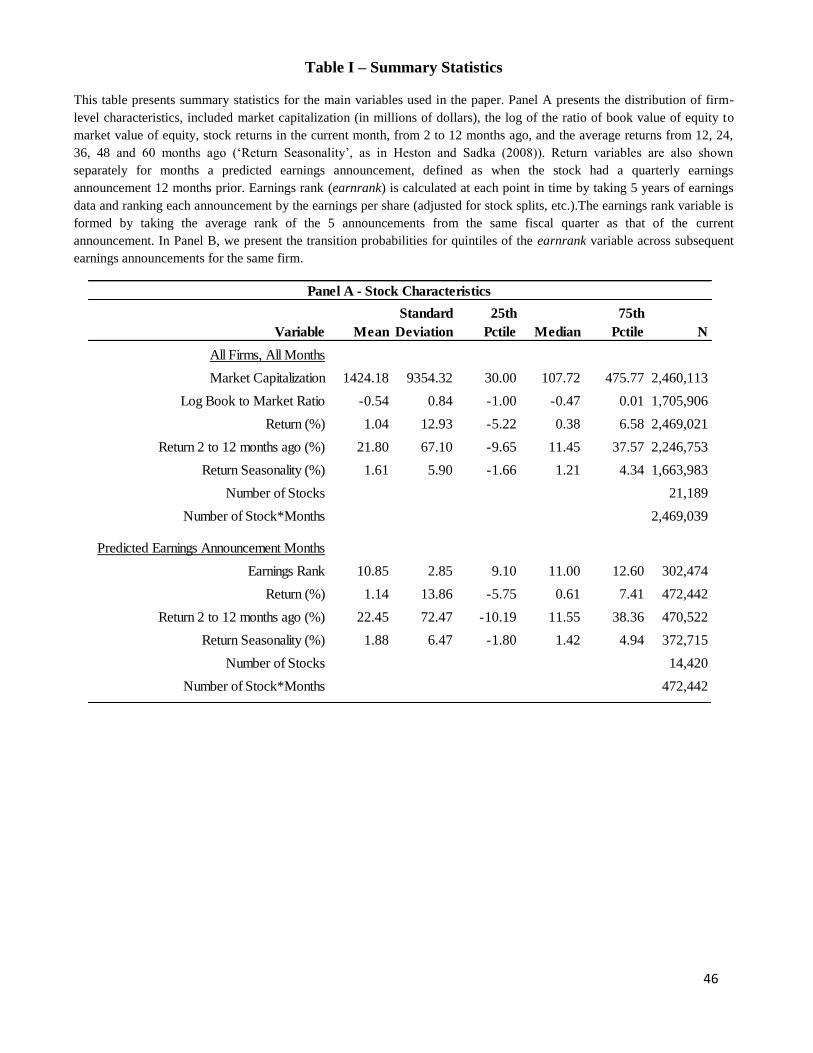
46

Variable Mean

Standard

Deviation

25th

Pctile Median

75th

Pctile N

All Firms, All Months

Market Capitalization 1424.18 9354.32 30.00 107.72 475.77 2,460,113

Log Book to Market Ratio -0.54 0.84 -1.00 -0.47 0.01 1,705,906

Return (%) 1.04 12.93 -5.22 0.38 6.58 2,469,021

Return 2 to 12 months ago (%) 21.80 67.10 -9.65 11.45 37.57 2,246,753

Return Seasonality (%) 1.61 5.90 -1.66 1.21 4.34 1,663,983

Number of Stocks 21,189

Number of Stock*Months 2,469,039

Predicted Earnings Announcement Months

Earnings Rank 10.85 2.85 9.10 11.00 12.60 302,474

Return (%) 1.14 13.86 -5.75 0.61 7.41 472,442

Return 2 to 12 months ago (%) 22.45 72.47 -10.19 11.55 38.36 470,522

Return Seasonality (%) 1.88 6.47 -1.80 1.42 4.94 372,715

Number of Stocks 14,420

Number of Stock*Months 472,442

Panel A - Stock Characteristics

Table I – Summary Statistics

This table presents summary statistics for the main variables used in the paper. Panel A presents the distribution of firm-

level characteristics, included market capitalization (in millions of dollars), the log of the ratio of book value of equity to

market value of equity, stock returns in the current month, from 2 to 12 months ago, and the average returns from 12, 24,

36, 48 and 60 months ago (‘Return Seasonality’, as in Heston and Sadka (2008)). Return variables are also shown

separately for months a predicted earnings announcement, defined as when the stock had a quarterly earnings

announcement 12 months prior. Earnings rank (earnrank) is calculated at each point in time by taking 5 years of earnings

data and ranking each announcement by the earnings per share (adjusted for stock splits, etc.).The earnings rank variable is

formed by taking the average rank of the 5 announcements from the same fiscal quarter as that of the current

announcement. In Panel B, we present the transition probabilities for quintiles of the earnrank variable across subsequent

earnings announcements for the same firm.

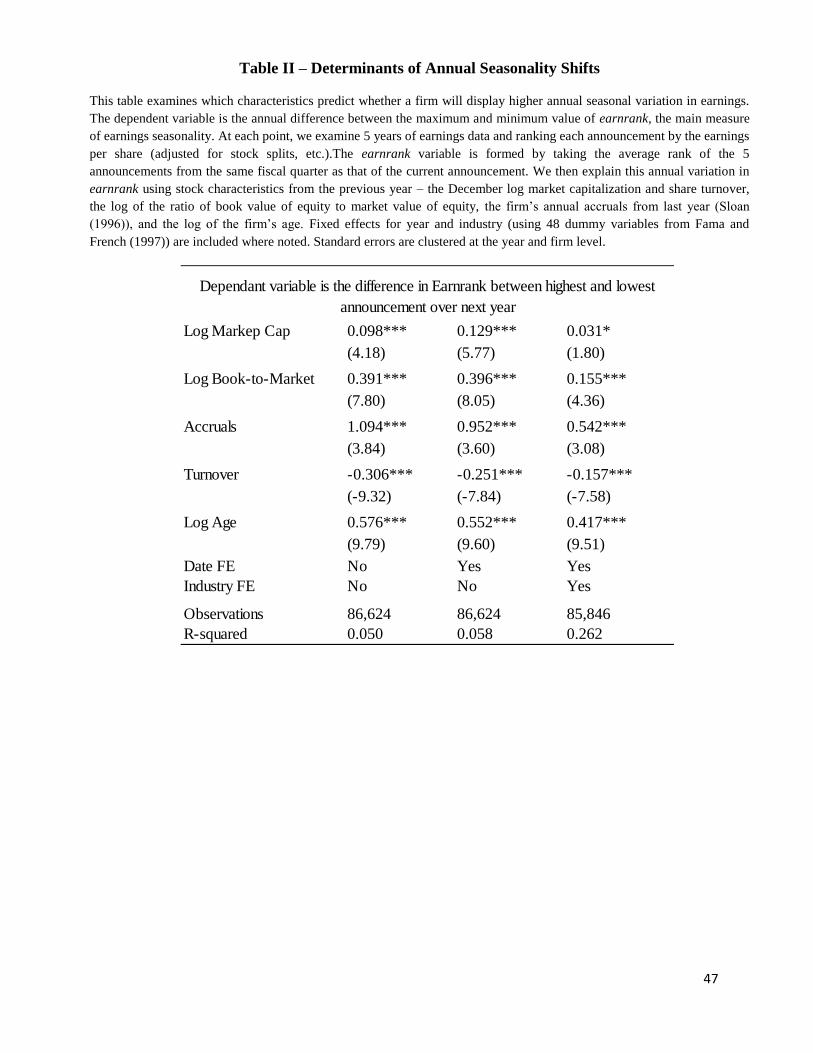
47

Log Markep Cap 0.098*** 0.129*** 0.031*

(4.18) (5.77) (1.80)

Log Book-to-Market 0.391*** 0.396*** 0.155***

(7.80) (8.05) (4.36)

Accruals 1.094*** 0.952*** 0.542***

(3.84) (3.60) (3.08)

Turnover -0.306*** -0.251*** -0.157***

(-9.32) (-7.84) (-7.58)

Log Age 0.576*** 0.552*** 0.417***

(9.79) (9.60) (9.51)

Date FE No Yes Yes

Industry FE No No Yes

Observations 86,624 86,624 85,846

R-squared 0.050 0.058 0.262

Dependant variable is the difference in Earnrank between highest and lowest

announcement over next year

Table II – Determinants of Annual Seasonality Shifts

This table examines which characteristics predict whether a firm will display higher annual seasonal variation in earnings.

The dependent variable is the annual difference between the maximum and minimum value of earnrank, the main measure

of earnings seasonality. At each point, we examine 5 years of earnings data and ranking each announcement by the earnings

per share (adjusted for stock splits, etc.).The earnrank variable is formed by taking the average rank of the 5

announcements from the same fiscal quarter as that of the current announcement. We then explain this annual variation in

earnrank using stock characteristics from the previous year – the December log market capitalization and share turnover,

the log of the ratio of book value of equity to market value of equity, the firm’s annual accruals from last year (Sloan

(1996)), and the log of the firm’s age. Fixed effects for year and industry (using 48 dummy variables from Fama and

French (1997)) are included where noted. Standard errors are clustered at the year and firm level.

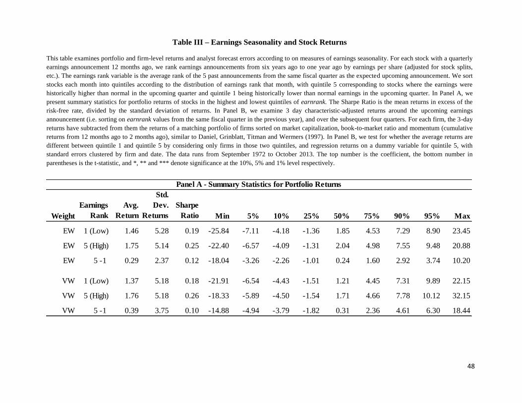
48

Weight

Earnings

Rank

Avg.

Return

Std.

Dev.

Returns

Sharpe

Ratio Min 5% 10% 25% 50% 75% 90% 95% Max

EW 1 (Low) 1.46 5.28 0.19 -25.84 -7.11 -4.18 -1.36 1.85 4.53 7.29 8.90 23.45

EW 5 (High) 1.75 5.14 0.25 -22.40 -6.57 -4.09 -1.31 2.04 4.98 7.55 9.48 20.88

EW 5 -1 0.29 2.37 0.12 -18.04 -3.26 -2.26 -1.01 0.24 1.60 2.92 3.74 10.20

VW 1 (Low) 1.37 5.18 0.18 -21.91 -6.54 -4.43 -1.51 1.21 4.45 7.31 9.89 22.15

VW 5 (High) 1.76 5.18 0.26 -18.33 -5.89 -4.50 -1.54 1.71 4.66 7.78 10.12 32.15

VW 5 -1 0.39 3.75 0.10 -14.88 -4.94 -3.79 -1.82 0.31 2.36 4.61 6.30 18.44

Panel A - Summary Statistics for Portfolio Returns

Table III – Earnings Seasonality and Stock Returns

This table examines portfolio and firm-level returns and analyst forecast errors according to on measures of earnings seasonality. For each stock with a quarterly

earnings announcement 12 months ago, we rank earnings announcements from six years ago to one year ago by earnings per share (adjusted for stock splits,

etc.). The earnings rank variable is the average rank of the 5 past announcements from the same fiscal quarter as the expected upcoming announcement. We sort

stocks each month into quintiles according to the distribution of earnings rank that month, with quintile 5 corresponding to stocks where the earnings were

historically higher than normal in the upcoming quarter and quintile 1 being historically lower than normal earnings in the upcoming quarter. In Panel A, we

present summary statistics for portfolio returns of stocks in the highest and lowest quintiles of earnrank. The Sharpe Ratio is the mean returns in excess of the

risk-free rate, divided by the standard deviation of returns. In Panel B, we examine 3 day characteristic-adjusted returns around the upcoming earnings

announcement (i.e. sorting on earnrank values from the same fiscal quarter in the previous year), and over the subsequent four quarters. For each firm, the 3-day

returns have subtracted from them the returns of a matching portfolio of firms sorted on market capitalization, book-to-market ratio and momentum (cumulative

returns from 12 months ago to 2 months ago), similar to Daniel, Grinblatt, Titman and Wermers (1997). In Panel B, we test for whether the average returns are

different between quintile 1 and quintile 5 by considering only firms in those two quintiles, and regression returns on a dummy variable for quintile 5, with

standard errors clustered by firm and date. The data runs from September 1972 to October 2013. The top number is the coefficient, the bottom number in

parentheses is the t-statistic, and *, ** and *** denote significance at the 10%, 5% and 1% level respectively.

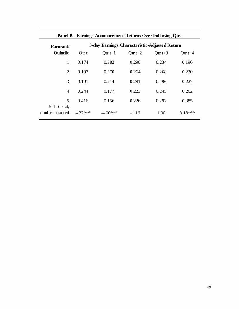
49

Qtr t Qtr t+1 Qtr t+2 Qtr t+3 Qtr t+4

1 0.174 0.382 0.290 0.234 0.196

2 0.197 0.270 0.264 0.268 0.230

3 0.191 0.214 0.281 0.196 0.227

4 0.244 0.177 0.223 0.245 0.262

5 0.416 0.156 0.226 0.292 0.385

5-1 t -stat,

double clustered 4.32*** -4.00*** -1.16 1.00 3.18***

Panel B - Earnings Announcement Returns Over Following Qtrs

Earnrank

Quintile

3-day Earnings Characteristic-Adjusted Return

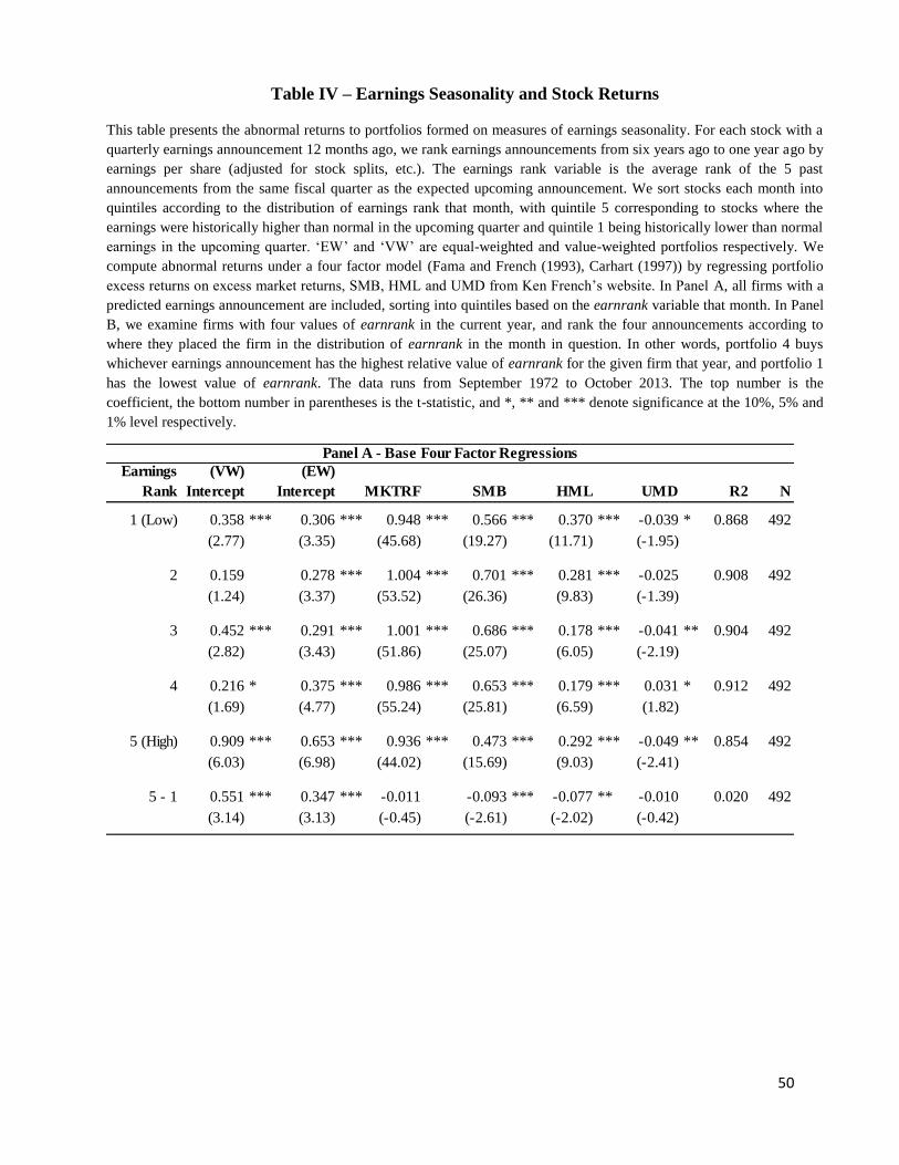
50

Earnings

Rank

(VW)

Intercept

(EW)

Intercept MKTRF SMB HML UMD R2 N

1 (Low) 0.358 *** 0.306 *** 0.948 *** 0.566 *** 0.370 *** -0.039 * 0.868 492

(2.77) (3.35) (45.68) (19.27) (11.71) (-1.95)

2 0.159 0.278 *** 1.004 *** 0.701 *** 0.281 *** -0.025 0.908 492

(1.24) (3.37) (53.52) (26.36) (9.83) (-1.39)

3 0.452 *** 0.291 *** 1.001 *** 0.686 *** 0.178 *** -0.041 ** 0.904 492

(2.82) (3.43) (51.86) (25.07) (6.05) (-2.19)

4 0.216 * 0.375 *** 0.986 *** 0.653 *** 0.179 *** 0.031 * 0.912 492

(1.69) (4.77) (55.24) (25.81) (6.59) (1.82)

5 (High) 0.909 *** 0.653 *** 0.936 *** 0.473 *** 0.292 *** -0.049 ** 0.854 492

(6.03) (6.98) (44.02) (15.69) (9.03) (-2.41)

5 - 1 0.551 *** 0.347 *** -0.011 -0.093 *** -0.077 ** -0.010 0.020 492

(3.14) (3.13) (-0.45) (-2.61) (-2.02) (-0.42)

Panel A - Base Four Factor Regressions

Table IV – Earnings Seasonality and Stock Returns

This table presents the abnormal returns to portfolios formed on measures of earnings seasonality. For each stock with a

quarterly earnings announcement 12 months ago, we rank earnings announcements from six years ago to one year ago by

earnings per share (adjusted for stock splits, etc.). The earnings rank variable is the average rank of the 5 past

announcements from the same fiscal quarter as the expected upcoming announcement. We sort stocks each month into

quintiles according to the distribution of earnings rank that month, with quintile 5 corresponding to stocks where the

earnings were historically higher than normal in the upcoming quarter and quintile 1 being historically lower than normal

earnings in the upcoming quarter. ‘EW’ and ‘VW’ are equal-weighted and value-weighted portfolios respectively. We

compute abnormal returns under a four factor model (Fama and French (1993), Carhart (1997)) by regressing portfolio

excess returns on excess market returns, SMB, HML and UMD from Ken French’s website. In Panel A, all firms with a

predicted earnings announcement are included, sorting into quintiles based on the earnrank variable that month. In Panel

B, we examine firms with four values of earnrank in the current year, and rank the four announcements according to

where they placed the firm in the distribution of earnrank in the month in question. In other words, portfolio 4 buys

whichever earnings announcement has the highest relative value of earnrank for the given firm that year, and portfolio 1

has the lowest value of earnrank. The data runs from September 1972 to October 2013. The top number is the

coefficient, the bottom number in parentheses is the t-statistic, and *, ** and *** denote significance at the 10%, 5% and

1% level respectively.

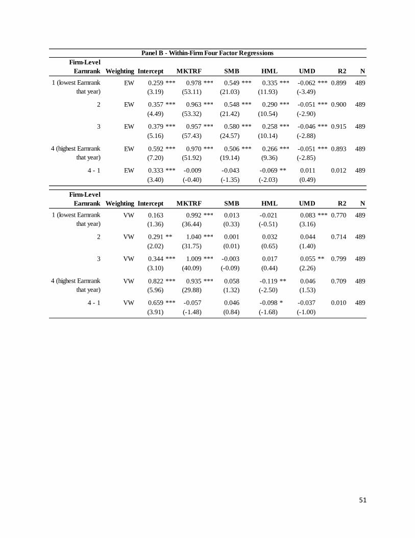
51

Firm-Level

Earnrank Weighting Intercept MKTRF SMB HML UMD R2 N

EW 0.259 *** 0.978 *** 0.549 *** 0.335 *** -0.062 *** 0.899 489

(3.19) (53.11) (21.03) (11.93) (-3.49)

2 EW 0.357 *** 0.963 *** 0.548 *** 0.290 *** -0.051 *** 0.900 489

(4.49) (53.32) (21.42) (10.54) (-2.90)

3 EW 0.379 *** 0.957 *** 0.580 *** 0.258 *** -0.046 *** 0.915 489

(5.16) (57.43) (24.57) (10.14) (-2.88)

EW 0.592 *** 0.970 *** 0.506 *** 0.266 *** -0.051 *** 0.893 489

(7.20) (51.92) (19.14) (9.36) (-2.85)

4 - 1 EW 0.333 *** -0.009 -0.043 -0.069 ** 0.011 0.012 489

(3.40) (-0.40) (-1.35) (-2.03) (0.49)

Firm-Level

Earnrank Weighting Intercept MKTRF SMB HML UMD R2 N

VW 0.163 0.992 *** 0.013 -0.021 0.083 *** 0.770 489

(1.36) (36.44) (0.33) (-0.51) (3.16)

2 VW 0.291 ** 1.040 *** 0.001 0.032 0.044 0.714 489

(2.02) (31.75) (0.01) (0.65) (1.40)

3 VW 0.344 *** 1.009 *** -0.003 0.017 0.055 ** 0.799 489

(3.10) (40.09) (-0.09) (0.44) (2.26)

VW 0.822 *** 0.935 *** 0.058 -0.119 ** 0.046 0.709 489

(5.96) (29.88) (1.32) (-2.50) (1.53)

4 - 1 VW 0.659 *** -0.057 0.046 -0.098 * -0.037 0.010 489

(3.91) (-1.48) (0.84) (-1.68) (-1.00)

4 (highest Earnrank

that year)

Panel B - Within-Firm Four Factor Regressions

1 (lowest Earnrank

that year)

4 (highest Earnrank

that year)

1 (lowest Earnrank

that year)

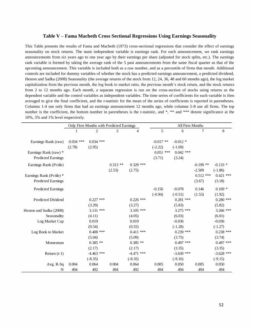
52

1 2 3 4 5 6 7 8

Earnings Rank (raw) 0.034 *** 0.034 *** -0.017 ** -0.012 *

(2.78) (2.95) (-2.22) (-1.69)

0.051 *** 0.042 ***

(3.71) (3.24)

Earnings Rank (Pctile) 0.313 ** 0.329 *** -0.199 ** -0.133 *

(2.53) (2.75) -2.509 (-1.86)

0.512 *** 0.421 ***

(3.67) (3.18)

Predicted Earnings -0.156 -0.078 0.146 0.169 *

(-0.94) (-0.51) (1.53) (1.92)

Predicted Dividend 0.227 *** 0.226 *** 0.281 *** 0.280 ***

(3.29) (3.27) (5.83) (5.82)

3.131 *** 3.105 *** 3.275 *** 3.266 ***

(4.11) (4.05) (6.03) (6.01)

Log Market Cap 0.019 0.019 -0.036 -0.036

(0.54) (0.55) (-1.28) (-1.27)

Log Book to Market 0.408 *** 0.411 *** 0.239 *** 0.238 ***

(5.04) (5.09) (3.75) (3.74)

Momentum 0.385 ** 0.385 ** 0.497 *** 0.497 ***

(2.17) (2.17) (3.35) (3.35)

Return (t-1) -4.463 *** -4.471 *** -3.630 *** -3.628 ***

(-8.35) (-8.35) (-9.16) (-9.15)

Avg. R-Sq 0.004 0.064 0.004 0.064 0.005 0.050 0.005 0.050

N 494 492 494 492 494 494 494 494

Earnings Rank (Pctile) *

Predicted Earnings

Only Firm Months with Predicted Earnings All Firm Months

Earnings Rank (raw) *

Predicted Earnings

Heston and Sadka (2008)

Seasonality

Table V – Fama Macbeth Cross Sectional Regressions Using Earnings Seasonality

This Table presents the results of Fama and Macbeth (1973) cross-sectional regressions that consider the effect of earnings

seasonality on stock returns. The main independent variable is earnings rank. For each announcement, we rank earnings

announcements from six years ago to one year ago by their earnings per share (adjusted for stock splits, etc.). The earnings

rank variable is formed by taking the average rank of the 5 past announcements from the same fiscal quarter as that of the

upcoming announcement. This variable is included both as a raw number, and as a percentile of firms that month. Additional

controls are included for dummy variables of whether the stock has a predicted earnings announcement, a predicted dividend,

Heston and Sadka (2008) Seasonality (the average returns of the stock from 12, 24, 36, 48 and 60 months ago), the log market

capitalization from the previous month, the log book to market ratio, the previous month’s stock return, and the stock returns

from 2 to 12 months ago. Each month, a separate regression is run on the cross-section of stocks using returns as the

dependent variable and the control variables as independent variables. The time series of coefficients for each variable is then

averaged to give the final coefficient, and the t-statistic for the mean of the series of coefficients is reported in parentheses.

Columns 1-4 use only firms that had an earnings announcement 12 months ago, while columns 5-8 use all firms. The top

number is the coefficient, the bottom number in parentheses is the t-statistic, and *, ** and *** denote significance at the

10%, 5% and 1% level respectively.

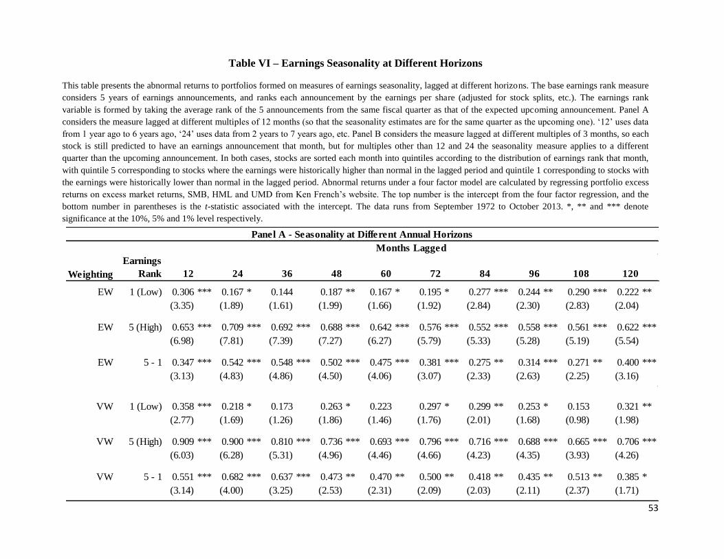
53

Weighting

Earnings

Rank 12 24 36 48 60 72 84 96 108 120

EW 1 (Low) 0.306 *** 0.167 * 0.144 0.187 ** 0.167 * 0.195 * 0.277 *** 0.244 ** 0.290 *** 0.222 **

(3.35) (1.89) (1.61) (1.99) (1.66) (1.92) (2.84) (2.30) (2.83) (2.04)

EW 5 (High) 0.653 *** 0.709 *** 0.692 *** 0.688 *** 0.642 *** 0.576 *** 0.552 *** 0.558 *** 0.561 *** 0.622 ***

(6.98) (7.81) (7.39) (7.27) (6.27) (5.79) (5.33) (5.28) (5.19) (5.54)

EW 5 - 1 0.347 *** 0.542 *** 0.548 *** 0.502 *** 0.475 *** 0.381 *** 0.275 ** 0.314 *** 0.271 ** 0.400 ***

(3.13) (4.83) (4.86) (4.50) (4.06) (3.07) (2.33) (2.63) (2.25) (3.16)

VW 1 (Low) 0.358 *** 0.218 * 0.173 0.263 * 0.223 0.297 * 0.299 ** 0.253 * 0.153 0.321 **

(2.77) (1.69) (1.26) (1.86) (1.46) (1.76) (2.01) (1.68) (0.98) (1.98)

VW 5 (High) 0.909 *** 0.900 *** 0.810 *** 0.736 *** 0.693 *** 0.796 *** 0.716 *** 0.688 *** 0.665 *** 0.706 ***

(6.03) (6.28) (5.31) (4.96) (4.46) (4.66) (4.23) (4.35) (3.93) (4.26)

VW 5 - 1 0.551 *** 0.682 *** 0.637 *** 0.473 ** 0.470 ** 0.500 ** 0.418 ** 0.435 ** 0.513 ** 0.385 *

(3.14) (4.00) (3.25) (2.53) (2.31) (2.09) (2.03) (2.11) (2.37) (1.71)

Months Lagged

Panel A - Seasonality at Different Annual Horizons

Table VI – Earnings Seasonality at Different Horizons

This table presents the abnormal returns to portfolios formed on measures of earnings seasonality, lagged at different horizons. The base earnings rank measure

considers 5 years of earnings announcements, and ranks each announcement by the earnings per share (adjusted for stock splits, etc.). The earnings rank

variable is formed by taking the average rank of the 5 announcements from the same fiscal quarter as that of the expected upcoming announcement. Panel A

considers the measure lagged at different multiples of 12 months (so that the seasonality estimates are for the same quarter as the upcoming one). ‘12’ uses data

from 1 year ago to 6 years ago, ‘24’ uses data from 2 years to 7 years ago, etc. Panel B considers the measure lagged at different multiples of 3 months, so each

stock is still predicted to have an earnings announcement that month, but for multiples other than 12 and 24 the seasonality measure applies to a different

quarter than the upcoming announcement. In both cases, stocks are sorted each month into quintiles according to the distribution of earnings rank that month,

with quintile 5 corresponding to stocks where the earnings were historically higher than normal in the lagged period and quintile 1 corresponding to stocks with

the earnings were historically lower than normal in the lagged period. Abnormal returns under a four factor model are calculated by regressing portfolio excess

returns on excess market returns, SMB, HML and UMD from Ken French’s website. The top number is the intercept from the four factor regression, and the

bottom number in parentheses is the t-statistic associated with the intercept. The data runs from September 1972 to October 2013. *, ** and *** denote

significance at the 10%, 5% and 1% level respectively.

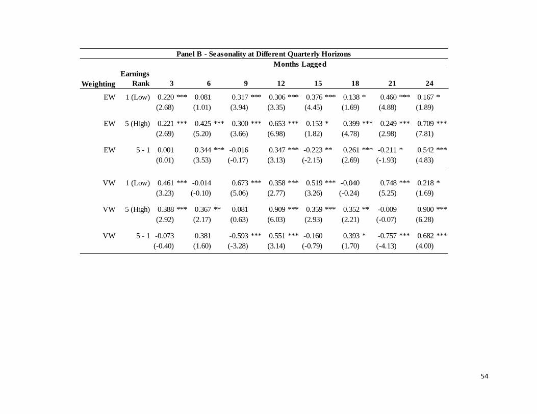
54

Weighting

Earnings

Rank 3 6 9 12 15 18 21 24

EW 1 (Low) 0.220 *** 0.081 0.317 *** 0.306 *** 0.376 *** 0.138 * 0.460 *** 0.167 *

(2.68) (1.01) (3.94) (3.35) (4.45) (1.69) (4.88) (1.89)

EW 5 (High) 0.221 *** 0.425 *** 0.300 *** 0.653 *** 0.153 * 0.399 *** 0.249 *** 0.709 ***

(2.69) (5.20) (3.66) (6.98) (1.82) (4.78) (2.98) (7.81)

EW 5 - 1 0.001 0.344 *** -0.016 0.347 *** -0.223 ** 0.261 *** -0.211 * 0.542 ***

(0.01) (3.53) (-0.17) (3.13) (-2.15) (2.69) (-1.93) (4.83)

VW 1 (Low) 0.461 *** -0.014 0.673 *** 0.358 *** 0.519 *** -0.040 0.748 *** 0.218 *

(3.23) (-0.10) (5.06) (2.77) (3.26) (-0.24) (5.25) (1.69)

VW 5 (High) 0.388 *** 0.367 ** 0.081 0.909 *** 0.359 *** 0.352 ** -0.009 0.900 ***

(2.92) (2.17) (0.63) (6.03) (2.93) (2.21) (-0.07) (6.28)

VW 5 - 1 -0.073 0.381 -0.593 *** 0.551 *** -0.160 0.393 * -0.757 *** 0.682 ***

(-0.40) (1.60) (-3.28) (3.14) (-0.79) (1.70) (-4.13) (4.00)

Months Lagged

Panel B - Seasonality at Different Quarterly Horizons

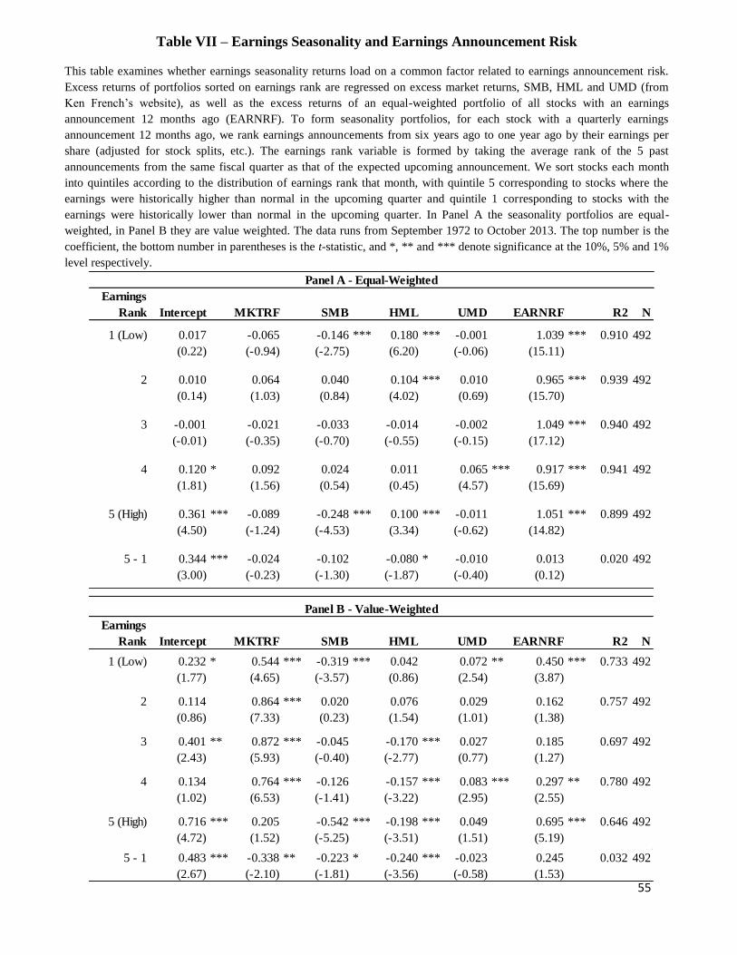
55

Earnings

Rank Intercept MKTRF SMB HML UMD EARNRF R2 N

1 (Low) 0.017 -0.065 -0.146 *** 0.180 *** -0.001 1.039 *** 0.910 492

(0.22) (-0.94) (-2.75) (6.20) (-0.06) (15.11)

2 0.010 0.064 0.040 0.104 *** 0.010 0.965 *** 0.939 492

(0.14) (1.03) (0.84) (4.02) (0.69) (15.70)

3 -0.001 -0.021 -0.033 -0.014 -0.002 1.049 *** 0.940 492

(-0.01) (-0.35) (-0.70) (-0.55) (-0.15) (17.12)

4 0.120 * 0.092 0.024 0.011 0.065 *** 0.917 *** 0.941 492

(1.81) (1.56) (0.54) (0.45) (4.57) (15.69)

5 (High) 0.361 *** -0.089 -0.248 *** 0.100 *** -0.011 1.051 *** 0.899 492

(4.50) (-1.24) (-4.53) (3.34) (-0.62) (14.82)

5 - 1 0.344 *** -0.024 -0.102 -0.080 * -0.010 0.013 0.020 492

(3.00) (-0.23) (-1.30) (-1.87) (-0.40) (0.12)

Panel A - Equal-Weighted

Earnings

Rank Intercept MKTRF SMB HML UMD EARNRF R2 N

1 (Low) 0.232 * 0.544 *** -0.319 *** 0.042 0.072 ** 0.450 *** 0.733 492

(1.77) (4.65) (-3.57) (0.86) (2.54) (3.87)

2 0.114 0.864 *** 0.020 0.076 0.029 0.162 0.757 492

(0.86) (7.33) (0.23) (1.54) (1.01) (1.38)

3 0.401 ** 0.872 *** -0.045 -0.170 *** 0.027 0.185 0.697 492

(2.43) (5.93) (-0.40) (-2.77) (0.77) (1.27)

4 0.134 0.764 *** -0.126 -0.157 *** 0.083 *** 0.297 ** 0.780 492

(1.02) (6.53) (-1.41) (-3.22) (2.95) (2.55)

5 (High) 0.716 *** 0.205 -0.542 *** -0.198 *** 0.049 0.695 *** 0.646 492

(4.72) (1.52) (-5.25) (-3.51) (1.51) (5.19)

5 - 1 0.483 *** -0.338 ** -0.223 * -0.240 *** -0.023 0.245 0.032 492

(2.67) (-2.10) (-1.81) (-3.56) (-0.58) (1.53)

Panel B - Value-Weighted

Table VII – Earnings Seasonality and Earnings Announcement Risk

This table examines whether earnings seasonality returns load on a common factor related to earnings announcement risk.

Excess returns of portfolios sorted on earnings rank are regressed on excess market returns, SMB, HML and UMD (from

Ken French’s website), as well as the excess returns of an equal-weighted portfolio of all stocks with an earnings

announcement 12 months ago (EARNRF). To form seasonality portfolios, for each stock with a quarterly earnings

announcement 12 months ago, we rank earnings announcements from six years ago to one year ago by their earnings per

share (adjusted for stock splits, etc.). The earnings rank variable is formed by taking the average rank of the 5 past

announcements from the same fiscal quarter as that of the expected upcoming announcement. We sort stocks each month

into quintiles according to the distribution of earnings rank that month, with quintile 5 corresponding to stocks where the

earnings were historically higher than normal in the upcoming quarter and quintile 1 corresponding to stocks with the

earnings were historically lower than normal in the upcoming quarter. In Panel A the seasonality portfolios are equal-

weighted, in Panel B they are value weighted. The data runs from September 1972 to October 2013. The top number is the

coefficient, the bottom number in parentheses is the t-statistic, and *, ** and *** denote significance at the 10%, 5% and 1%

level respectively.

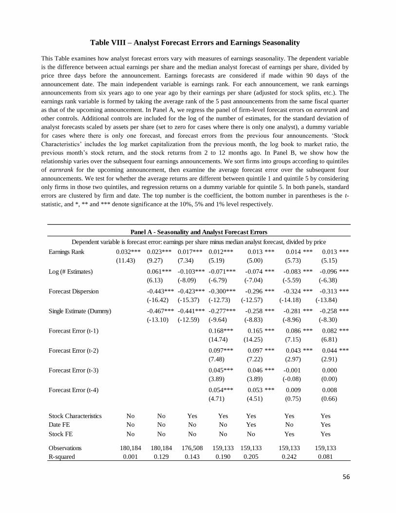
56

Table VIII – Analyst Forecast Errors and Earnings Seasonality

This Table examines how analyst forecast errors vary with measures of earnings seasonality. The dependent variable

is the difference between actual earnings per share and the median analyst forecast of earnings per share, divided by

price three days before the announcement. Earnings forecasts are considered if made within 90 days of the

announcement date. The main independent variable is earnings rank. For each announcement, we rank earnings

announcements from six years ago to one year ago by their earnings per share (adjusted for stock splits, etc.). The

earnings rank variable is formed by taking the average rank of the 5 past announcements from the same fiscal quarter

as that of the upcoming announcement. In Panel A, we regress the panel of firm-level forecast errors on earnrank and

other controls. Additional controls are included for the log of the number of estimates, for the standard deviation of

analyst forecasts scaled by assets per share (set to zero for cases where there is only one analyst), a dummy variable

for cases where there is only one forecast, and forecast errors from the previous four announcements. ‘Stock

Characteristics’ includes the log market capitalization from the previous month, the log book to market ratio, the

previous month’s stock return, and the stock returns from 2 to 12 months ago. In Panel B, we show how the

relationship varies over the subsequent four earnings announcements. We sort firms into groups according to quintiles

of earnrank for the upcoming announcement, then examine the average forecast error over the subsequent four

announcements. We test for whether the average returns are different between quintile 1 and quintile 5 by considering

only firms in those two quintiles, and regression returns on a dummy variable for quintile 5. In both panels, standard

errors are clustered by firm and date. The top number is the coefficient, the bottom number in parentheses is the t-

statistic, and *, ** and *** denote significance at the 10%, 5% and 1% level respectively.

Earnings Rank 0.032*** 0.023*** 0.017*** 0.012*** 0.013 *** 0.014 *** 0.013 ***

(11.43) (9.27) (7.34) (5.19) (5.00) (5.73) (5.15)

Log (# Estimates) 0.061*** -0.103*** -0.071*** -0.074 *** -0.083 *** -0.096 ***

(6.13) (-8.09) (-6.79) (-7.04) (-5.59) (-6.38)

Forecast Dispersion -0.443*** -0.423*** -0.300*** -0.296 *** -0.324 *** -0.313 ***

(-16.42) (-15.37) (-12.73) (-12.57) (-14.18) (-13.84)

Single Estimate (Dummy) -0.467*** -0.441*** -0.277*** -0.258 *** -0.281 *** -0.258 ***

(-13.10) (-12.59) (-9.64) (-8.83) (-8.96) (-8.30)

Forecast Error (t-1) 0.168*** 0.165 *** 0.086 *** 0.082 ***

(14.74) (14.25) (7.15) (6.81)

Forecast Error (t-2) 0.097*** 0.097 *** 0.043 *** 0.044 ***

(7.48) (7.22) (2.97) (2.91)

Forecast Error (t-3) 0.045*** 0.046 *** -0.001 0.000

(3.89) (3.89) (-0.08) (0.00)

Forecast Error (t-4) 0.054*** 0.053 *** 0.009 0.008

(4.71) (4.51) (0.75) (0.66)

Stock Characteristics No No Yes Yes Yes Yes Yes

Date FE No No No No Yes No Yes

Stock FE No No No No No Yes Yes

Observations 180,184 180,184 176,508 159,133 159,133 159,133 159,133

R-squared 0.001 0.129 0.143 0.190 0.205 0.242 0.081

Dependent variable is forecast error: earnings per share minus median analyst forecast, divided by price

Panel A - Seasonality and Analyst Forecast Errors

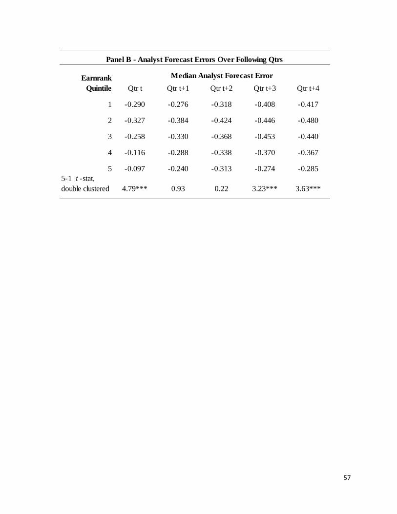
57

Qtr t Qtr t+1 Qtr t+2 Qtr t+3 Qtr t+4

1 -0.290 -0.276 -0.318 -0.408 -0.417

2 -0.327 -0.384 -0.424 -0.446 -0.480

3 -0.258 -0.330 -0.368 -0.453 -0.440

4 -0.116 -0.288 -0.338 -0.370 -0.367

5 -0.097 -0.240 -0.313 -0.274 -0.285

5-1 t -stat,

double clustered 4.79*** 0.93 0.22 3.23*** 3.63***

Panel B - Analyst Forecast Errors Over Following Qtrs

Earnrank

Quintile

Median Analyst Forecast Error

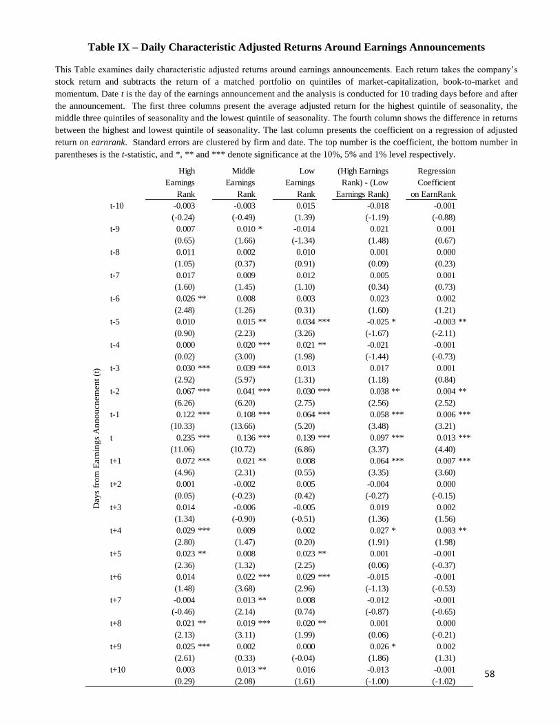
58

High

Earnings

Rank

Middle

Earnings

Rank

Low

Earnings

Rank

(High Earnings

Rank) - (Low

Earnings Rank)

Regression

Coefficient

on EarnRank

t-10 -0.003 -0.003 0.015 -0.018 -0.001

(-0.24) (-0.49) (1.39) (-1.19) (-0.88)

t-9 0.007 0.010 * -0.014 0.021 0.001

(0.65) (1.66) (-1.34) (1.48) (0.67)

t-8 0.011 0.002 0.010 0.001 0.000

(1.05) (0.37) (0.91) (0.09) (0.23)

t-7 0.017 0.009 0.012 0.005 0.001

(1.60) (1.45) (1.10) (0.34) (0.73)

t-6 0.026 ** 0.008 0.003 0.023 0.002

(2.48) (1.26) (0.31) (1.60) (1.21)

t-5 0.010 0.015 ** 0.034 *** -0.025 * -0.003 **

(0.90) (2.23) (3.26) (-1.67) (-2.11)

t-4 0.000 0.020 *** 0.021 ** -0.021 -0.001

(0.02) (3.00) (1.98) (-1.44) (-0.73)

t-3 0.030 *** 0.039 *** 0.013 0.017 0.001

(2.92) (5.97) (1.31) (1.18) (0.84)

t-2 0.067 *** 0.041 *** 0.030 *** 0.038 ** 0.004 **

(6.26) (6.20) (2.75) (2.56) (2.52)

t-1 0.122 *** 0.108 *** 0.064 *** 0.058 *** 0.006 ***

(10.33) (13.66) (5.20) (3.48) (3.21)

t 0.235 *** 0.136 *** 0.139 *** 0.097 *** 0.013 ***

(11.06) (10.72) (6.86) (3.37) (4.40)

t+1 0.072 *** 0.021 ** 0.008 0.064 *** 0.007 ***

(4.96) (2.31) (0.55) (3.35) (3.60)

t+2 0.001 -0.002 0.005 -0.004 0.000

(0.05) (-0.23) (0.42) (-0.27) (-0.15)

t+3 0.014 -0.006 -0.005 0.019 0.002

(1.34) (-0.90) (-0.51) (1.36) (1.56)

t+4 0.029 *** 0.009 0.002 0.027 * 0.003 **

(2.80) (1.47) (0.20) (1.91) (1.98)

t+5 0.023 ** 0.008 0.023 ** 0.001 -0.001

(2.36) (1.32) (2.25) (0.06) (-0.37)

t+6 0.014 0.022 *** 0.029 *** -0.015 -0.001

(1.48) (3.68) (2.96) (-1.13) (-0.53)

t+7 -0.004 0.013 ** 0.008 -0.012 -0.001

(-0.46) (2.14) (0.74) (-0.87) (-0.65)

t+8 0.021 ** 0.019 *** 0.020 ** 0.001 0.000

(2.13) (3.11) (1.99) (0.06) (-0.21)

t+9 0.025 *** 0.002 0.000 0.026 * 0.002

(2.61) (0.33) (-0.04) (1.86) (1.31)

t+10 0.003 0.013 ** 0.016 -0.013 -0.001

(0.29) (2.08) (1.61) (-1.00) (-1.02)

Day

s fr

om

Earn

ing

s A

nn

ou

cn

em

en

t (t

)

Table IX – Daily Characteristic Adjusted Returns Around Earnings Announcements

This Table examines daily characteristic adjusted returns around earnings announcements. Each return takes the company’s

stock return and subtracts the return of a matched portfolio on quintiles of market-capitalization, book-to-market and

momentum. Date t is the day of the earnings announcement and the analysis is conducted for 10 trading days before and after

the announcement. The first three columns present the average adjusted return for the highest quintile of seasonality, the

middle three quintiles of seasonality and the lowest quintile of seasonality. The fourth column shows the difference in returns

between the highest and lowest quintile of seasonality. The last column presents the coefficient on a regression of adjusted

return on earnrank. Standard errors are clustered by firm and date. The top number is the coefficient, the bottom number in

parentheses is the t-statistic, and *, ** and *** denote significance at the 10%, 5% and 1% level respectively.

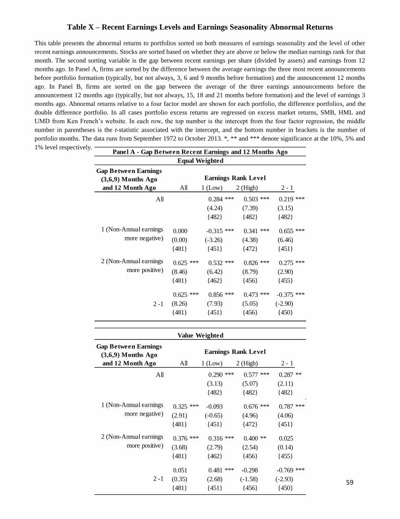
59

All 1 (Low) 2 (High) 2 - 1

All 0.284 *** 0.503 *** 0.219 ***

(4.24) (7.39) (3.15)

{482} {482} {482}

0.000 -0.315 *** 0.341 *** 0.655 ***

(0.00) (-3.26) (4.38) (6.46)

{481} {451} {472} {451}

0.625 *** 0.532 *** 0.826 *** 0.275 ***

(8.46) (6.42) (8.79) (2.90)

{481} {462} {456} {455}

0.625 *** 0.856 *** 0.473 *** -0.375 ***

(8.26) (7.93) (5.05) (-2.90)

{481} {451} {456} {450}

All 1 (Low) 2 (High) 2 - 1

All 0.290 *** 0.577 *** 0.287 **

(3.13) (5.07) (2.11)

{482} {482} {482}

0.325 *** -0.093 0.676 *** 0.787 ***

(2.91) (-0.65) (4.96) (4.06)

{481} {451} {472} {451}

0.376 *** 0.316 *** 0.400 ** 0.025

(3.68) (2.79) (2.54) (0.14)

{481} {462} {456} {455}

0.051 0.481 *** -0.298 -0.769 ***

(0.35) (2.68) (-1.58) (-2.93)

{481} {451} {456} {450}

2 (Non-Annual earnings

more positive)

2 -1

Panel A - Gap Between Recent Earnings and 12 Months Ago

2 -1

Value Weighted

Gap Between Earnings

(3,6,9) Months Ago

and 12 Month Ago

Earnings Rank Level

1 (Non-Annual earnings

more negative)

2 (Non-Annual earnings

more positive)

Equal Weighted

Gap Between Earnings

(3,6,9) Months Ago

and 12 Month Ago

Earnings Rank Level

1 (Non-Annual earnings

more negative)

Table X – Recent Earnings Levels and Earnings Seasonality Abnormal Returns

This table presents the abnormal returns to portfolios sorted on both measures of earnings seasonality and the level of other

recent earnings announcements. Stocks are sorted based on whether they are above or below the median earnings rank for that

month. The second sorting variable is the gap between recent earnings per share (divided by assets) and earnings from 12

months ago. In Panel A, firms are sorted by the difference between the average earnings the three most recent announcements

before portfolio formation (typically, but not always, 3, 6 and 9 months before formation) and the announcement 12 months

ago. In Panel B, firms are sorted on the gap between the average of the three earnings announcements before the

announcement 12 months ago (typically, but not always, 15, 18 and 21 months before formation) and the level of earnings 3

months ago. Abnormal returns relative to a four factor model are shown for each portfolio, the difference portfolios, and the

double difference portfolio. In all cases portfolio excess returns are regressed on excess market returns, SMB, HML and

UMD from Ken French’s website. In each row, the top number is the intercept from the four factor regression, the middle

number in parentheses is the t-statistic associated with the intercept, and the bottom number in brackets is the number of

portfolio months. The data runs from September 1972 to October 2013. *, ** and *** denote significance at the 10%, 5% and

1% level respectively.

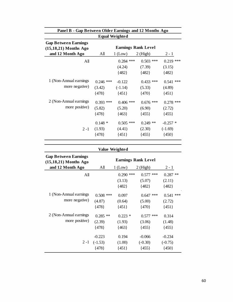
60

All 1 (Low) 2 (High) 2 - 1

All 0.284 *** 0.503 *** 0.219 ***

(4.24) (7.39) (3.15)

{482} {482} {482}

0.246 *** -0.122 0.433 *** 0.541 ***

(3.42) (-1.14) (5.33) (4.89)

{478} {451} {470} {451}

0.393 *** 0.406 *** 0.676 *** 0.278 ***

(5.82) (5.20) (6.90) (2.72)

{478} {463} {455} {455}

0.148 * 0.505 *** 0.249 ** -0.257 *

(1.93) (4.41) (2.30) (-1.69)

{478} {451} {455} {450}

All 1 (Low) 2 (High) 2 - 1

All 0.290 *** 0.577 *** 0.287 **

(3.13) (5.07) (2.11)

{482} {482} {482}

0.508 *** 0.097 0.647 *** 0.541 ***

(4.87) (0.64) (5.00) (2.72)

{478} {451} {470} {451}

0.285 ** 0.223 * 0.577 *** 0.314

(2.39) (1.93) (3.06) (1.48)

{478} {463} {455} {455}

-0.223 0.194 -0.066 -0.234

(-1.53) (1.00) (-0.30) (-0.75)

{478} {451} {455} {450}

1 (Non-Annual earnings

more negative)

2 (Non-Annual earnings

more positive)

2 -1

2 (Non-Annual earnings

more positive)

2 -1

Value Weighted

Gap Between Earnings

(15,18,21) Months Ago

and 12 Month Ago

Earnings Rank Level

1 (Non-Annual earnings

more negative)

Panel B - Gap Between Older Earnings and 12 Months Ago

Equal Weighted

Gap Between Earnings

(15,18,21) Months Ago

and 12 Month Ago

Earnings Rank Level

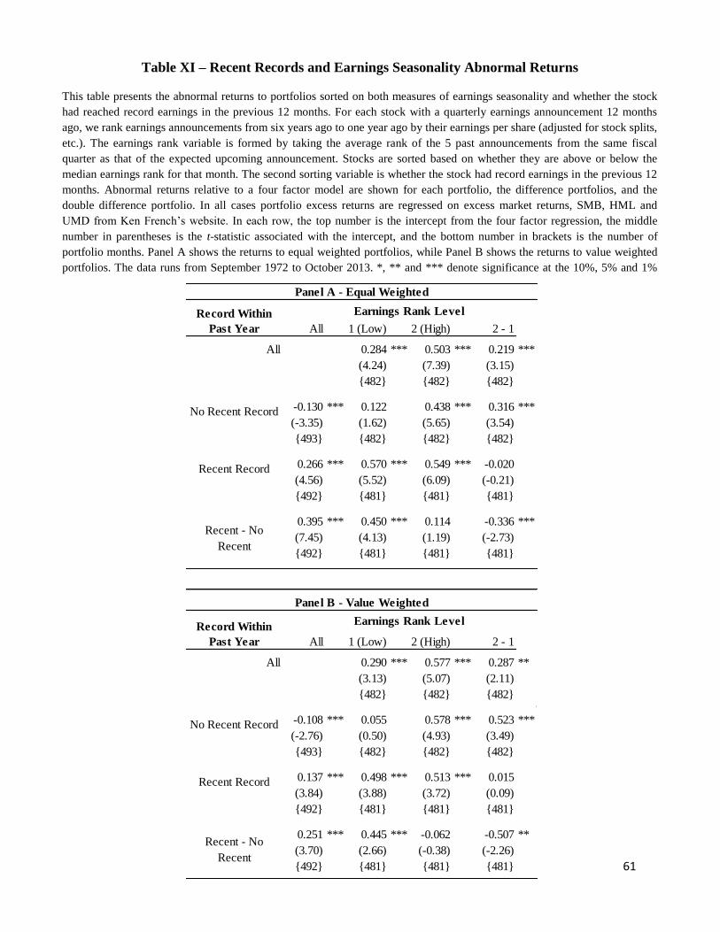
61

All 1 (Low) 2 (High) 2 - 1

All 0.284 *** 0.503 *** 0.219 ***

(4.24) (7.39) (3.15)

{482} {482} {482}

-0.130 *** 0.122 0.438 *** 0.316 ***

(-3.35) (1.62) (5.65) (3.54)

{493} {482} {482} {482}

0.266 *** 0.570 *** 0.549 *** -0.020

(4.56) (5.52) (6.09) (-0.21)

{492} {481} {481} {481}

0.395 *** 0.450 *** 0.114 -0.336 ***

(7.45) (4.13) (1.19) (-2.73)

{492} {481} {481} {481}

All 1 (Low) 2 (High) 2 - 1

All 0.290 *** 0.577 *** 0.287 **

(3.13) (5.07) (2.11)

{482} {482} {482}

-0.108 *** 0.055 0.578 *** 0.523 ***

(-2.76) (0.50) (4.93) (3.49)

{493} {482} {482} {482}

0.137 *** 0.498 *** 0.513 *** 0.015

(3.84) (3.88) (3.72) (0.09)

{492} {481} {481} {481}

0.251 *** 0.445 *** -0.062 -0.507 **

(3.70) (2.66) (-0.38) (-2.26)

{492} {481} {481} {481}

Recent - No

Recent

Record Within

Past Year

Panel A - Equal Weighted

Earnings Rank Level

Record Within

Past Year

Recent Record

No Recent Record

Recent Record

Recent - No

Recent

Panel B - Value Weighted

Earnings Rank Level

No Recent Record

Table XI – Recent Records and Earnings Seasonality Abnormal Returns

This table presents the abnormal returns to portfolios sorted on both measures of earnings seasonality and whether the stock

had reached record earnings in the previous 12 months. For each stock with a quarterly earnings announcement 12 months

ago, we rank earnings announcements from six years ago to one year ago by their earnings per share (adjusted for stock splits,

etc.). The earnings rank variable is formed by taking the average rank of the 5 past announcements from the same fiscal

quarter as that of the expected upcoming announcement. Stocks are sorted based on whether they are above or below the

median earnings rank for that month. The second sorting variable is whether the stock had record earnings in the previous 12

months. Abnormal returns relative to a four factor model are shown for each portfolio, the difference portfolios, and the

double difference portfolio. In all cases portfolio excess returns are regressed on excess market returns, SMB, HML and

UMD from Ken French’s website. In each row, the top number is the intercept from the four factor regression, the middle

number in parentheses is the t-statistic associated with the intercept, and the bottom number in brackets is the number of

portfolio months. Panel A shows the returns to equal weighted portfolios, while Panel B shows the returns to value weighted

portfolios. The data runs from September 1972 to October 2013. *, ** and *** denote significance at the 10%, 5% and 1%

level respectively.

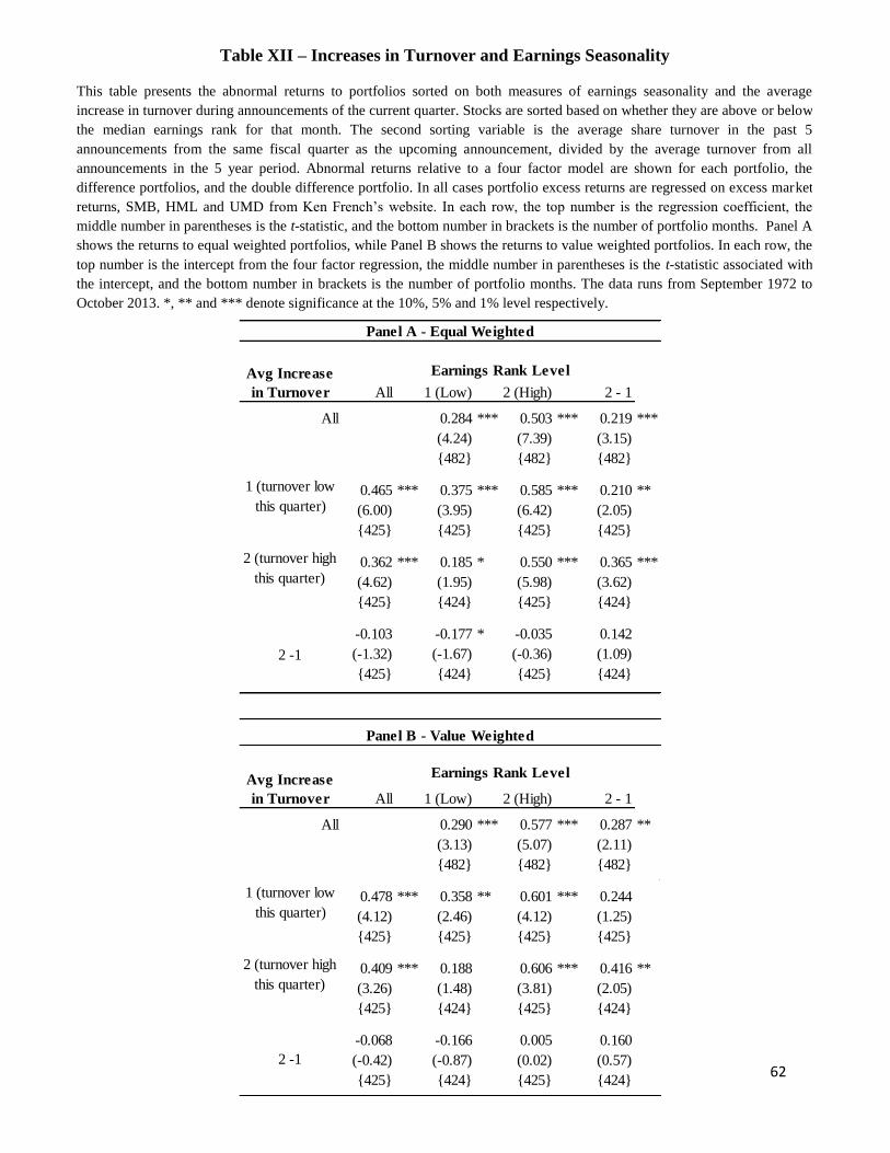
62

All 1 (Low) 2 (High) 2 - 1

All 0.284 *** 0.503 *** 0.219 ***

(4.24) (7.39) (3.15)

{482} {482} {482}

0.465 *** 0.375 *** 0.585 *** 0.210 **

(6.00) (3.95) (6.42) (2.05)

{425} {425} {425} {425}

0.362 *** 0.185 * 0.550 *** 0.365 ***

(4.62) (1.95) (5.98) (3.62)

{425} {424} {425} {424}

-0.103 -0.177 * -0.035 0.142

(-1.32) (-1.67) (-0.36) (1.09)

{425} {424} {425} {424}

All 1 (Low) 2 (High) 2 - 1

All 0.290 *** 0.577 *** 0.287 **

(3.13) (5.07) (2.11)

{482} {482} {482}

0.478 *** 0.358 ** 0.601 *** 0.244

(4.12) (2.46) (4.12) (1.25)

{425} {425} {425} {425}

0.409 *** 0.188 0.606 *** 0.416 **

(3.26) (1.48) (3.81) (2.05)

{425} {424} {425} {424}

-0.068 -0.166 0.005 0.160

(-0.42) (-0.87) (0.02) (0.57)

{425} {424} {425} {424}

2 (turnover high

this quarter)

2 -1

2 -1

Panel B - Value Weighted

Avg Increase

in Turnover

Earnings Rank Level

1 (turnover low

this quarter)

2 (turnover high

this quarter)

Panel A - Equal Weighted

Avg Increase

in Turnover

Earnings Rank Level

1 (turnover low

this quarter)

Table XII – Increases in Turnover and Earnings Seasonality

This table presents the abnormal returns to portfolios sorted on both measures of earnings seasonality and the average

increase in turnover during announcements of the current quarter. Stocks are sorted based on whether they are above or below

the median earnings rank for that month. The second sorting variable is the average share turnover in the past 5

announcements from the same fiscal quarter as the upcoming announcement, divided by the average turnover from all

announcements in the 5 year period. Abnormal returns relative to a four factor model are shown for each portfolio, the

difference portfolios, and the double difference portfolio. In all cases portfolio excess returns are regressed on excess market

returns, SMB, HML and UMD from Ken French’s website. In each row, the top number is the regression coefficient, the

middle number in parentheses is the t-statistic, and the bottom number in brackets is the number of portfolio months. Panel A

shows the returns to equal weighted portfolios, while Panel B shows the returns to value weighted portfolios. In each row, the

top number is the intercept from the four factor regression, the middle number in parentheses is the t-statistic associated with

the intercept, and the bottom number in brackets is the number of portfolio months. The data runs from September 1972 to

October 2013. *, ** and *** denote significance at the 10%, 5% and 1% level respectively.

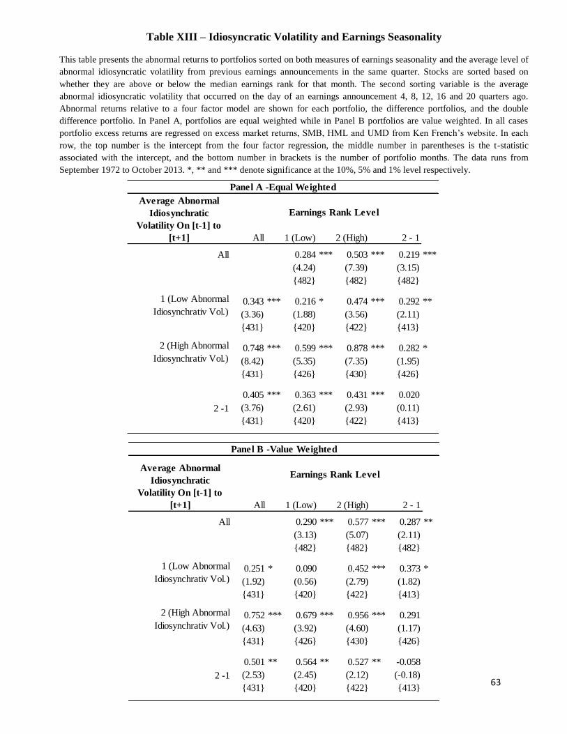
63

All 1 (Low) 2 (High) 2 - 1

All 0.284 *** 0.503 *** 0.219 ***

(4.24) (7.39) (3.15)

{482} {482} {482}

0.343 *** 0.216 * 0.474 *** 0.292 **

(3.36) (1.88) (3.56) (2.11)

{431} {420} {422} {413}

0.748 *** 0.599 *** 0.878 *** 0.282 *

(8.42) (5.35) (7.35) (1.95)

{431} {426} {430} {426}

0.405 *** 0.363 *** 0.431 *** 0.020

(3.76) (2.61) (2.93) (0.11)

{431} {420} {422} {413}

Panel A -Equal Weighted

2 (High Abnormal

Idiosynchrativ Vol.)

2 -1

Average Abnormal

Idiosynchratic

Volatility On [t-1] to

[t+1]

Earnings Rank Level

1 (Low Abnormal

Idiosynchrativ Vol.)

All 1 (Low) 2 (High) 2 - 1

All 0.290 *** 0.577 *** 0.287 **

(3.13) (5.07) (2.11)

{482} {482} {482}

0.251 * 0.090 0.452 *** 0.373 *

(1.92) (0.56) (2.79) (1.82)

{431} {420} {422} {413}

0.752 *** 0.679 *** 0.956 *** 0.291

(4.63) (3.92) (4.60) (1.17)

{431} {426} {430} {426}

0.501 ** 0.564 ** 0.527 ** -0.058

(2.53) (2.45) (2.12) (-0.18)

{431} {420} {422} {413}

Panel B -Value Weighted

2 (High Abnormal

Idiosynchrativ Vol.)

2 -1

Average Abnormal

Idiosynchratic

Volatility On [t-1] to

[t+1]

Earnings Rank Level

1 (Low Abnormal

Idiosynchrativ Vol.)

Table XIII – Idiosyncratic Volatility and Earnings Seasonality

This table presents the abnormal returns to portfolios sorted on both measures of earnings seasonality and the average level of

abnormal idiosyncratic volatility from previous earnings announcements in the same quarter. Stocks are sorted based on

whether they are above or below the median earnings rank for that month. The second sorting variable is the average

abnormal idiosyncratic volatility that occurred on the day of an earnings announcement 4, 8, 12, 16 and 20 quarters ago.

Abnormal returns relative to a four factor model are shown for each portfolio, the difference portfolios, and the double

difference portfolio. In Panel A, portfolios are equal weighted while in Panel B portfolios are value weighted. In all cases

portfolio excess returns are regressed on excess market returns, SMB, HML and UMD from Ken French’s website. In each

row, the top number is the intercept from the four factor regression, the middle number in parentheses is the t-statistic

associated with the intercept, and the bottom number in brackets is the number of portfolio months. The data runs from

September 1972 to October 2013. *, ** and *** denote significance at the 10%, 5% and 1% level respectively.

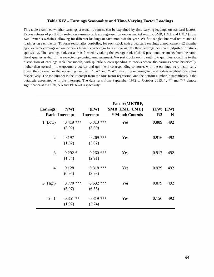
64

Earnings

Rank

(VW)

Intercept

(EW)

Intercept

Factor (MKTRF,

SMB, HML, UMD)

* Month Controls

(EW)

R2

(EW)

N

1 (Low) 0.419 *** 0.313 *** Yes 0.889 492

(3.02) (3.30)

2 0.197 0.269 *** Yes 0.916 492

(1.52) (3.02)

3 0.292 * 0.260 *** Yes 0.917 492

(1.84) (2.91)

4 0.128 0.318 *** Yes 0.929 492

(0.95) (3.98)

5 (High) 0.770 *** 0.632 *** Yes 0.879 492

(5.07) (6.55)

5 - 1 0.351 ** 0.319 *** Yes 0.156 492

(1.97) (2.74)

Table XIV – Earnings Seasonality and Time-Varying Factor Loadings

This table examines whether earnings seasonality returns can be explained by time-varying loadings on standard factors.

Excess returns of portfolios sorted on earnings rank are regressed on excess market returns, SMB, HML and UMD (from

Ken French’s website), allowing for different loadings in each month of the year. We fit a single abnormal return and 12

loadings on each factor. To form seasonality portfolios, for each stock with a quarterly earnings announcement 12 months

ago, we rank earnings announcements from six years ago to one year ago by their earnings per share (adjusted for stock

splits, etc.). The earnings rank variable is formed by taking the average rank of the 5 past announcements from the same

fiscal quarter as that of the expected upcoming announcement. We sort stocks each month into quintiles according to the

distribution of earnings rank that month, with quintile 5 corresponding to stocks where the earnings were historically

higher than normal in the upcoming quarter and quintile 1 corresponding to stocks with the earnings were historically

lower than normal in the upcoming quarter. . ‘EW’ and ‘VW’ refer to equal-weighted and value-weighted portfolios

respectively. The top number is the intercept from the four factor regression, and the bottom number in parentheses is the

t-statistic associated with the intercept. The data runs from September 1972 to October 2013. *, ** and *** denote

significance at the 10%, 5% and 1% level respectively.

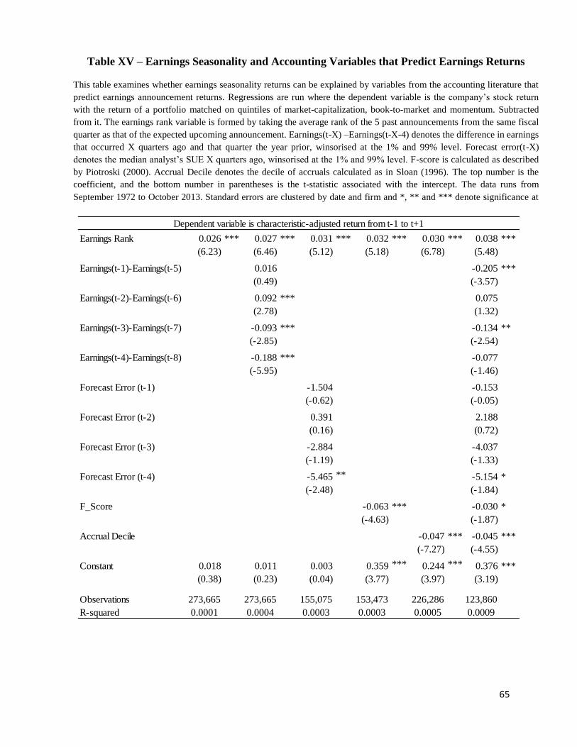
65

Earnings Rank 0.026 *** 0.027 *** 0.031 *** 0.032 *** 0.030 *** 0.038 ***

(6.23) (6.46) (5.12) (5.18) (6.78) (5.48)

Earnings(t-1)-Earnings(t-5) 0.016 -0.205 ***

(0.49) (-3.57)

Earnings(t-2)-Earnings(t-6) 0.092 *** 0.075

(2.78) (1.32)

Earnings(t-3)-Earnings(t-7) -0.093 *** -0.134 **

(-2.85) (-2.54)

Earnings(t-4)-Earnings(t-8) -0.188 *** -0.077

(-5.95) (-1.46)

Forecast Error (t-1) -1.504 -0.153

(-0.62) (-0.05)

Forecast Error (t-2) 0.391 2.188

(0.16) (0.72)

Forecast Error (t-3) -2.884 -4.037

(-1.19) (-1.33)

Forecast Error (t-4) -5.465 ** -5.154 *

(-2.48) (-1.84)

F_Score -0.063 *** -0.030 *

(-4.63) (-1.87)

Accrual Decile -0.047 *** -0.045 ***

(-7.27) (-4.55)

Constant 0.018 0.011 0.003 0.359 *** 0.244 *** 0.376 ***

(0.38) (0.23) (0.04) (3.77) (3.97) (3.19)

Observations 273,665 273,665 155,075 153,473 226,286 123,860

R-squared 0.0001 0.0004 0.0003 0.0003 0.0005 0.0009

Dependent variable is characteristic-adjusted return from t-1 to t+1

Table XV – Earnings Seasonality and Accounting Variables that Predict Earnings Returns

This table examines whether earnings seasonality returns can be explained by variables from the accounting literature that

predict earnings announcement returns. Regressions are run where the dependent variable is the company’s stock return

with the return of a portfolio matched on quintiles of market-capitalization, book-to-market and momentum. Subtracted

from it. The earnings rank variable is formed by taking the average rank of the 5 past announcements from the same fiscal

quarter as that of the expected upcoming announcement. Earnings(t-X) –Earnings(t-X-4) denotes the difference in earnings

that occurred X quarters ago and that quarter the year prior, winsorised at the 1% and 99% level. Forecast error(t-X)

denotes the median analyst’s SUE X quarters ago, winsorised at the 1% and 99% level. F-score is calculated as described

by Piotroski (2000). Accrual Decile denotes the decile of accruals calculated as in Sloan (1996). The top number is the

coefficient, and the bottom number in parentheses is the t-statistic associated with the intercept. The data runs from

September 1972 to October 2013. Standard errors are clustered by date and firm and *, ** and *** denote significance at

the 10%, 5% and 1% level respectively.