Embed Size (px)
Citation preview

Tom Copeland [email protected] Director, Monitor Corporate Finance www.corpfinonline.comMonitor Group, Cambridge, Massachusetts www.monitor.com
For more reading see:Copeland, T, T. Koller, J. Murrin, Valuation: Measuring and Managing the Value of Companies
Copyright © 2001 by Monitor Company Group, L.P.
No part of this publication may be reproduced, stored in a retrieval system, or transmitted in any form or by any means — electronic, mechanical, photocopying, recording, or otherwise — without the permission of Monitor Company Group, L.P.
This document provides an outline of a presentation and is incomplete without the accompanying oral commentary and discussion.
COMPANY CONFIDENTIAL
Trends in Valuation
NIVRA, Amsterdam, June 1, 2001

Copyright © 2001 Monitor Company Group LP — Confidential — CAMZKN-MFR-NIVRA 6 01-TEC 2
Changes in Value are at the Heart of Economic Decision-Making
Discounted Cash Flow Valuation DCF
Expectations-Based Management
Real Options Analysis
Discounted Cash Flow Valuation DCF Discounted Cash Flow Valuation DCF

Copyright © 2001 Monitor Company Group LP — Confidential — CAMZKN-MFR-NIVRA 6 01-TEC 3
Discounted Cash Flow Definition
DCF has three components:
Free Cash Flow = EBIT - Cash taxes on EBIT + accrued taxes due
+ depreciation – Capital Expenditures – operating working capital
WACC =
Continuing Value =
V
SK
V
BK Sb )rate tax marginal1(
gWACC
rgEBIT
)/1)(ratecash tax 1(

Copyright © 2001 Monitor Company Group LP — Confidential — CAMZKN-MFR-NIVRA 6 01-TEC 4
Source: Value Line forecasts; Copeland, Koller, Murrin, Valuation, 2nd edition, 1994
0.0
2.0
4.0
6.0
8.0
10.0
12.0
0 1 2 3 4 5 6 7 8 9 10
35 Large U.S. Companies, 1988
1988 DCF / Book
19
88
Ma
rke
t /
Bo
ok
R2 = 0.94
DCF Works Well For Large Publicly Held Companies
R2 = 0.92
0
5
10
15
0 5 10 15
1999 DCF / Book Value1
99
9 M
ark
et
/ B
oo
k V
alu
e
Source: Value Line Forecasts, Monitor Analysis
31 Large U.S. Companies, 1999

Copyright © 2001 Monitor Company Group LP — Confidential — CAMZKN-MFR-NIVRA 6 01-TEC 5
High Correlation Between Market Value and DCF Value
for 28 Japanese Companies — 1993
The R2 for 28 Japanese companies was 89 percent
Market / Book Value
0
1
2
3
4
5
0 1 2 3 4 5
DCF / Book (Using Value Line Forecasts)
R2 = 0.89
Comments:1. Underutilized land 2. Cross-holdings

Copyright © 2001 Monitor Company Group LP — Confidential — CAMZKN-MFR-NIVRA 6 01-TEC 6
. . . for 15 Italian companies (the R2 was 95.4 percent) . . .
DCF / Book
Market / Book Value
0.2
0.4
0.6
0.8
1.0
1.2
1.4
1.6
0.2 0.4 0.6 0.8 1.0 1.2 1.4 1.6
Correlation Between DCF and Market Value
for 15 Italian Companies* — 1990
Snia
Pirelli
Sip
Falk
Burgo
FiatMagneti M.
Montedison
Stet
FidenzaAuschen
Merloni
Cementir
Benetton
R2 = 0.954
2.0 3.0
2.0
3.0
Olivetti
Correlation between DCF and Market Value — Italy
* Using publicly available information** Capitalization on September 28, 1990 (Borsa valori di Milano), book value of companySource: Copeland, Koller and Murrin, Valuation
Comments:1. Mark to market inflation accounting2. Holder assets

Copyright © 2001 Monitor Company Group LP — Confidential — CAMZKN-MFR-NIVRA 6 01-TEC 7
Brazil

Copyright © 2001 Monitor Company Group LP — Confidential — CAMZKN-MFR-NIVRA 6 01-TEC 8
DCF Works Across Different Industries
16 banks
*5 banks are non-U.S. banksSource: Global Vantage; Value Line
Ma
rke
t /
Bo
ok
Va
lue
0.0
0.5
1.0
1.5
2.0
2.5
3.0
0.0 0.5 1.0 1.5 2.0 2.5 3.0
DCF / Book Value
R2 = 0.97
13 Insurance Companies
Mar
ket
/ Bo
ok
Val
ue
DCF / Book Value30 1 2
3
0
1
2
R2 = 0.92
1. Equity Approach2. Income model/ interest spread model
1. Equity Approach2. Unrealized capital gains

Copyright © 2001 Monitor Company Group LP — Confidential — CAMZKN-MFR-NIVRA 6 01-TEC 9
60
80
100
120
140
160
1804-
Jan-
99
13-J
an-9
9
25-J
an-9
9
3-F
eb-9
9
12-F
eb-9
9
24-F
eb-9
9
5-M
ar-9
9
16-M
ar-9
9
25-M
ar-9
9
6-A
pr-9
9
15-A
pr-9
9
26-A
pr-9
9
5-M
ay-9
9
14-M
ay-9
9
25-M
ay-9
9
4-Ju
n-99
15-J
un-9
9
24-J
un-9
9
6-Ju
l-99
15-J
ul-9
9
26-J
ul-9
9
4-A
ug-9
9
13-A
ug-9
9
24-A
ug-9
9
2-S
ep-9
9
14-S
ep-9
9
DCF Works for Robust Growth Companies
1999 Stock Price (AOL)
Note: 1999 elsewhere in valuation refers to FY 99 which ends in June Source: Compustat
Price Per Share
Volume(Millions)
0
10
20
30
40
50
60
4-Ja
n-99
13-J
an-9
9
25-J
an-9
9
3-F
eb-9
9
12-F
eb-9
9
24-F
eb-9
9
5-M
ar-9
9
16-M
ar-9
9
25-M
ar-9
9
6-A
pr-9
9
15-A
pr-9
9
26-A
pr-9
9
5-M
ay-9
9
14-M
ay-9
9
25-M
ay-9
9
4-Ju
n-99
15-J
un-9
9
24-J
un-9
9
6-Ju
l-99
15-J
ul-9
9
26-J
ul-9
9
4-A
ug-9
9
13-A
ug-9
9
24-A
ug-9
9
2-S
ep-9
9
14-S
ep-9
9
1999 Trading Volume (AOL)

Copyright © 2001 Monitor Company Group LP — Confidential — CAMZKN-MFR-NIVRA 6 01-TEC 10
AOL Revenue Assumptions for the Valuation Model Were Closely Tracked
to Analyst Estimates of Long Term Revenue Growth
$27,450
$25,183
$22,894
$20,260
$17,466
$12,233$9,945
$8,080$6,288
$4,777
$14,801
$0
$5,000
$10,000
$15,000
$20,000
$25,000
$30,000
1999 2000 2001 2002 2003 2004 2005 2006 2007 2008 2009
Revenue Growth
* Most analysts did not forecast beyond 2003Note: FY for AOL ends in JuneSource: ING Barings; BankBoston Robertson Stephens; Donaldson, Lufkin, and Jenrette
$ Billions
Deviation fromAnalystProjections*
1.5% 1.9% 2.3% 0.1%
1999-2004 Average Growth Rate: 25.4%
2004-2009 Average Growth Rate: 13.2%
Long-Term Revenue Growth: 9%
Copyright © 2001 Monitor Company Group LP — Confidential — CAMZKN-MFR-NIVRA 6 01-TEC 11
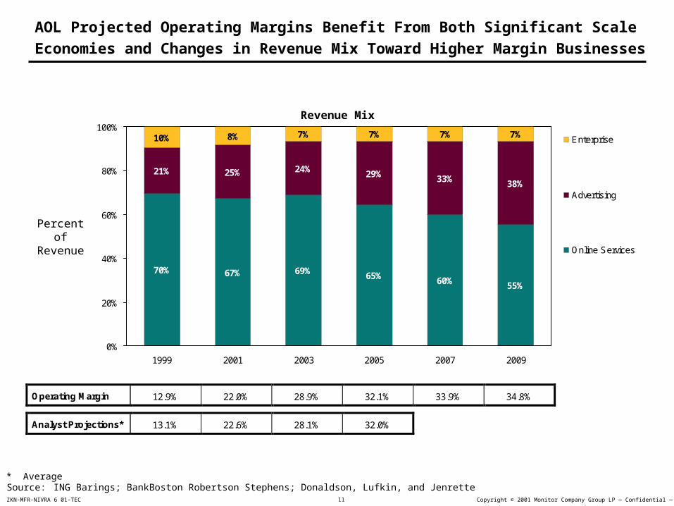
AOL Projected Operating Margins Benefit From Both Significant Scale
Economies and Changes in Revenue Mix Toward Higher Margin Businesses
70% 67% 69% 65% 60% 55%
21% 25% 24% 29% 33% 38%
10% 8% 7% 7% 7% 7%
0%
20%
40%
60%
80%
100%
1999 2001 2003 2005 2007 2009
Enterprise
Advertising
Online Services
Revenue Mix
Source: ING Barings; BankBoston Robertson Stephens; Donaldson, Lufkin, and Jenrette
Percent of Revenue
Operating Margin 12.9% 22.0% 28.9% 32.1% 33.9% 34.8%
Analyst Projections* 13.1% 22.6% 28.1% 32.0%
* Average
Copyright © 2001 Monitor Company Group LP — Confidential — CAMZKN-MFR-NIVRA 6 01-TEC 12
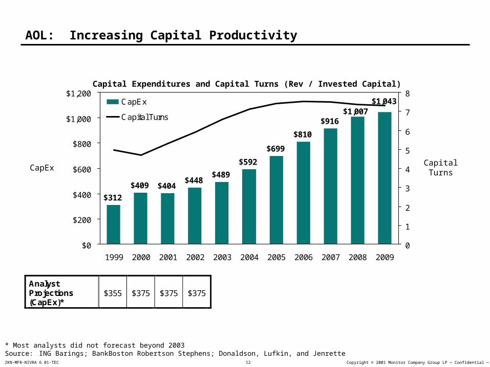
AnalystProjections(CapEx)*
$355 $375 $375 $375
AOL: Increasing Capital Productivity
Capital Expenditures and Capital Turns (Rev / Invested Capital)
* Most analysts did not forecast beyond 2003Source: ING Barings; BankBoston Robertson Stephens; Donaldson, Lufkin, and Jenrette
Capital Turns
CapEx
$312
$409 $404$448
$489
$592
$699
$810
$916$1,007
$1,043
$0
$200
$400
$600
$800
$1,000
$1,200
1999 2000 2001 2002 2003 2004 2005 2006 2007 2008 2009
0
1
2
3
4
5
6
7
8CapEx
Capital Turns

Copyright © 2001 Monitor Company Group LP — Confidential — CAMZKN-MFR-NIVRA 6 01-TEC 13
AOL: Matures Led to the Use of a Changing WACC
99.7%92.5%
85.4%
0.3%7.5%
14.6%0%
25%
50%
75%
100%
1999 2004 2009
Equity
Debt
AOL Capital Structure
Source: Compustat, Bloomberg, Monitor Analysis
Based on comparables taken from telecom, software, and news media
Equity Beta 1.69 1.38 1.06
Debt Rating B1 BBB3 A3
WACC 15.6% 13.5% 11.0%
Percent

Copyright © 2001 Monitor Company Group LP — Confidential — CAMZKN-MFR-NIVRA 6 01-TEC 14
AOL: Continuing Value
Return on New Investment
Continuing Value35% 40% 45%
8% $55,933 $58,038 $59,674
9% $80,934 $84,474 $87,228NOPLATGrowth
10% $155,025 $162,820 $168,883
In the base case shown below, continuing value contributes 85% of total operating value (approximately $76 out of $93 per share)
Continuing value growth rate has a particularly large impact because the growth rate is very close to the ending WACC of 11%
WACC = 11% in the long run
Copyright © 2001 Monitor Company Group LP — Confidential — CAMZKN-MFR-NIVRA 6 01-TEC 15
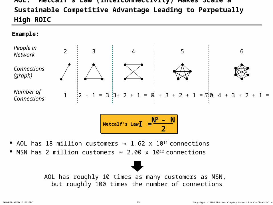
Example:
People in Network
2 3 4 5 6
Connections (graph)
Number of Connections
1 2 + 1 = 3 3+ 2 + 1 = 6 4 + 3 + 2 + 1 = 10 5 + 4 + 3 + 2 + 1 = 15
AOL: Metcalf’s Law (Interconnectivity) Makes Scale a Sustainable
Competitive Advantage Leading to Perpetually High ROIC
Metcalf’s Law:Metcalf’s Law: I =N2 - N
2
AOL has 18 million customers 1.62 x 10¹⁴ connections MSN has 2 million customers 2.00 x 10¹² connections
AOL has roughly 10 times as many customers as MSN, but roughly 100 times the number of connections

Copyright © 2001 Monitor Company Group LP — Confidential — CAMZKN-MFR-NIVRA 6 01-TEC 16
PV of FCF 1999-2009
PV of Continuing
Value
Marketable Securities and Non-operating
Assets
Debt Equity Value
AOL: The Changing WACC and Continuing Value Assumptions Bridge
the Analyst Projections and the Current Market Value
AOL Entity and Equity Value
Implied share price of $93 versus trading range of $89 to $104 between mid-August and mid-September
$MM $93 per Share$93 per Share$93 per Share$93 per Share
15,694
84,481 102,496
(348)
2,688
$0
$30,000
$60,000
$90,000
$120,000

Copyright © 2001 Monitor Company Group LP — Confidential — CAMZKN-MFR-NIVRA 6 01-TEC 17
AOL Market Ratios Decline Over Time as the Firm Matures
138.7
123.3
89.5
33.434.435.738.141.9
55.4
71.3
47.2
6.26.97.89.010.612.715.519.122.826.6
33.9
0
20
40
60
80
100
120
140
160
1999 2000 2001 2002 2003 2004 2005 2006 2007 2008 2009
Price to Earning and Price to Book
P/E Ratio
P/B Ratio

Copyright © 2001 Monitor Company Group LP — Confidential — CAMZKN-MFR-NIVRA 6 01-TEC 18
Amazon.com: Amazon’s Stock* (up to August 1999)
$42
$64
$37
$124
$100
$125
$119
$172$172
$117$107 $128
$0
$50
$100
$150
$200
Sep-98 Oct-98 Nov-98 Dec-98 Jan-99 Feb-99 Mar-99 Apr-99 May-99 Jun-99 Jul-99 Aug-99
* On August 12, 1999 Amazon.com undertook a 2 for 1 stock split. As our valuation reflects the value of the company in July 1999 we will use the number of outstanding shares before the split.
Dollars

Copyright © 2001 Monitor Company Group LP — Confidential — CAMZKN-MFR-NIVRA 6 01-TEC 19
Monitor’s Valuation Results: Amazon.com (July 1999)
$361 $349 $16,447$15,086
$1,329
$0
$5,000
$10,000
$15,000
$20,000
PV of FCF 1998-2008
PV of Continuing
Value
PV of Marketable Securities and Non-operating
Assets
Debt and Retirement-
relatedLiabilities
DCF Estimate of Equity
Value
$101 per Share$101 per Share$101 per Share$101 per Share
Note: Valuation as of July 1999 reflects pre-split price of $101/share. Trading range was $126.50 to $97.50

Copyright © 2001 Monitor Company Group LP — Confidential — CAMZKN-MFR-NIVRA 6 01-TEC 20
Summary Operating Assumptions July 1999
Monitor
Revenue Growth 2000 – 50%
2001 – 39.2%
2002 onward 39.2% declining to 21%
COGS / Revenue 2000 – 77%
2001 – 76%
2002 – 74%
SG&A / Revenue 2000 – 28%
2001 – 22.4%
2002 – 15% declining to 10.5%
Capex / Revenue 2000 – 2%
2001 – 1.5%
2002 – 1.5%
Net Working Capital /Revenue
2000 – - 16%
2001 – -17.5%
2002 – - 17.5%

Copyright © 2001 Monitor Company Group LP — Confidential — CAMZKN-MFR-NIVRA 6 01-TEC 21
Amazon.com Revenue Assumptions Were Closely Tracked to Analyst
Estimates Except for Donaldson, Lufkin & Jenrette
$0
$5,000
$10,000
$15,000
$20,000
$25,000
$30,000
1999 2000 2001 2002 2003 2004 2005 2006 2007 2008 2009
* Donaldson, Lufkin, and JenretteNote: Most analysts did not forecast beyond 2003
Revenue(In Millions)
1999-2004 Average Growth Rate: 40.5%
2004-2009 Average Growth Rate: 25.9%
Long-Term Revenue Growth: 9%
DL&J* Revenue Forecast

Copyright © 2001 Monitor Company Group LP — Confidential — CAMZKN-MFR-NIVRA 6 01-TEC 22
Amazon.com: Sensitivity Analysis of Price Per Share
Return on New Investment
Continuing ValueSensitivity 10% 11% 12%
9% $66 $102 $132
8% $66 $82 $95NOPLATGrowth
7% $66 $75 $83
92% of the Amazon’s market value is realized after the year 2009 and is reflected in the Continuous Value. The assumptions about the two parameters of Amazon’s Continuous Value: NOPLAT Growth and Return on New Investment are key to its valuation.
WACC = 10% in the long run

Copyright © 2001 Monitor Company Group LP — Confidential — CAMZKN-MFR-NIVRA 6 01-TEC 23
Amazon.com
Company TSR vs. S&P 500, 1999-2000
0
0.2
0.4
0.6
0.8
1
1.2
1.4
1.6
1.8
Dec-98
Jan-99
Feb-99
Mar-99
Apr-99
May-99
Jun-99
Jul-99
Aug-99
Sep-99
Oct-99
Nov-99
Dec-99
Jan-00
Feb-00
Mar-00
Apr-00
May-00
Jun-00
Jul-00
Aug-00
Sep-00
Oct-00
Nov-00
Dec-00
Jan-01
TR
S
Amazon
S&P 500

Copyright © 2001 Monitor Company Group LP — Confidential — CAMZKN-MFR-NIVRA 6 01-TEC 24
Amazon.com: Valuation Results July 1999 vs. January 2001
$ Million$ 15.3 per
share
$5,433
$2,114$1,045
$5,373
$1,130
0
1000
2000
3000
4000
5000
6000
7000
8000
9000
PV of FCF 2000 -2009
PV ofContinuing
Value
PV of ExcessCash and Non-
OperatingAssets
Total Debt DCF Estimate ofEquity Value
Value Build-Up January 2001
$15,086 $361 $349 $16,447
$1,329
$0
$5,000
$10,000
$15,000
$20,000
PV of FCF 1998-2008
PV of Continuing Value
PV of Marketable Securities and Non-operating Assets
Debt and Retirement-relatedLiabilities
DCF Estimate of Equity Value
$101 per Share$101 per Share$101 per Share$101 per Share
Note: Valuation as of July 1999 reflects pre-split price of $101/share.
Trading range was $126.50 to $97.50
Value Build-Up July 1999
Copyright © 2001 Monitor Company Group LP — Confidential — CAMZKN-MFR-NIVRA 6 01-TEC 25
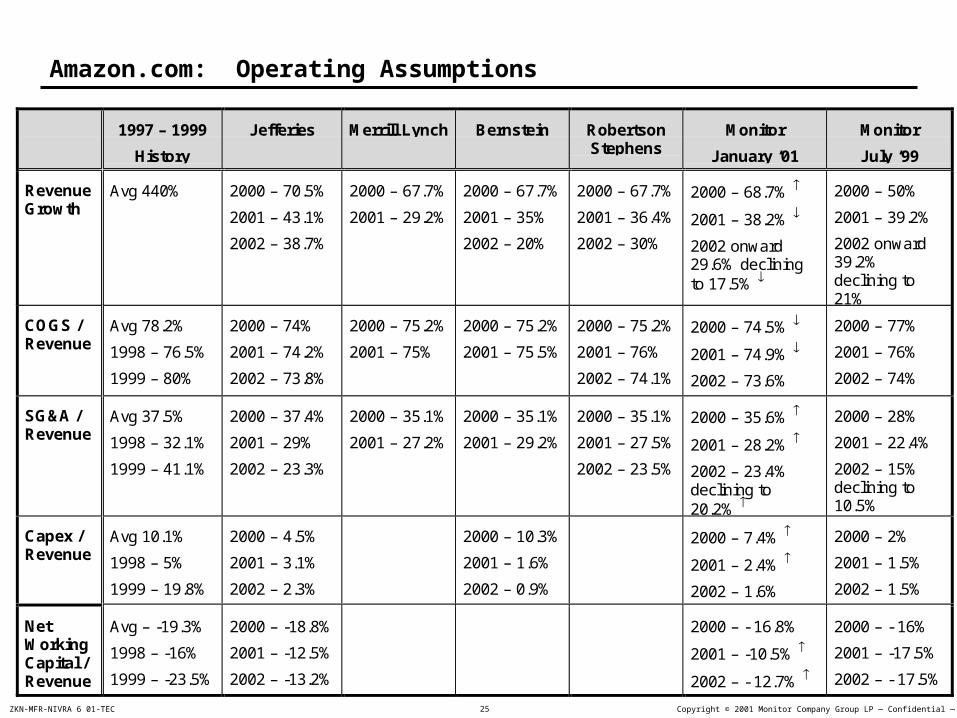
Amazon.com: Operating Assumptions
1997 – 1999
History
Jefferies Merrill Lynch Bernstein RobertsonStephens
Monitor
January ‘01
Monitor
July ‘99
RevenueGrowth
Avg 440% 2000 – 70.5%
2001 – 43.1%
2002 – 38.7%
2000 – 67.7%
2001 – 29.2%
2000 – 67.7%
2001 – 35%
2002 – 20%
2000 – 67.7%
2001 – 36.4%
2002 – 30%
2000 – 68.7%
2001 – 38.2%
2002 onward29.6% decliningto 17.5%
2000 – 50%
2001 – 39.2%
2002 onward39.2%declining to21%
COGS /Revenue
Avg 78.2%
1998 – 76.5%
1999 – 80%
2000 – 74%
2001 – 74.2%
2002 – 73.8%
2000 – 75.2%
2001 – 75%
2000 – 75.2%
2001 – 75.5%
2000 – 75.2%
2001 – 76%
2002 – 74.1%
2000 – 74.5%
2001 – 74.9%
2002 – 73.6%
2000 – 77%
2001 – 76%
2002 – 74%
SG&A /Revenue
Avg 37.5%
1998 – 32.1%
1999 – 41.1%
2000 – 37.4%
2001 – 29%
2002 – 23.3%
2000 – 35.1%
2001 – 27.2%
2000 – 35.1%
2001 – 29.2%
2000 – 35.1%
2001 – 27.5%
2002 – 23.5%
2000 – 35.6%
2001 – 28.2%
2002 – 23.4%declining to20.2%
2000 – 28%
2001 – 22.4%
2002 – 15%declining to10.5%
Capex /Revenue
Avg 10.1%
1998 – 5%
1999 – 19.8%
2000 – 4.5%
2001 – 3.1%
2002 – 2.3%
2000 – 10.3%
2001 – 1.6%
2002 – 0.9%
2000 – 7.4%
2001 – 2.4%
2002 – 1.6%
2000 – 2%
2001 – 1.5%
2002 – 1.5%
NetWorkingCapital /Revenue
Avg – -19.3%
1998 – -16%
1999 – -23.5%
2000 – -18.8%
2001 – -12.5%
2002 – -13.2%
2000 – - 16.8%
2001 – -10.5%
2002 – - 12.7%
2000 – - 16%
2001 – -17.5%
2002 – - 17.5%

Copyright © 2001 Monitor Company Group LP — Confidential — CAMZKN-MFR-NIVRA 6 01-TEC 26
Amazon.com: WACC & Continuing Value Assumptions
Monitor AssumptionsJanuary 2001
Monitor AssumptionsJuly 1999
WACC
Barra Beta
Risk Free Rate
Credit Rating
Pre-tax Cost of Debt
Cost of Equity
WACC
2.09
5.3%
B
10.9% (Debt / Total Capital(market value) 21.7%)
16.8% (Equity / Total Capital(market value) 78.3%)
14.5% declining to 10% by 2009
1.91
6.3%
B
11.8% (Debt / Total Capital(market value) 2.1%)
16.8% (Equity / Total Capital(market value) 97.9%)
16.6% declining to 10% by 2009
Continuing Value
Growth in NOPLAT
Return on Net NewInvestments
9%
11%
9%
11%

Copyright © 2001 Monitor Company Group LP — Confidential — CAMZKN-MFR-NIVRA 6 01-TEC 27
Changes in Value are at the Heart of Economic Decision-Making
Discounted Cash Flow Valuation DCF
Real Options Analysis
Expectations-Based Management Expectations-Based Management

Copyright © 2001 Monitor Company Group LP — Confidential — CAMZKN-MFR-NIVRA 6 01-TEC 28
Metric Critique
Sales Growth Ignores profitability, ignores balance sheet
EPS Ignores balance sheet
EPS Growth Ignores balance sheet
ROIC = EBIT / Invested Capital Encourages harvesting behavior
ROIC-WACC* Encourages harvesting
EVA=(ROIC-WACC) x Invested Capital Not correlated with TRS
Rational Expectations Best of short-term metrics
An Example:
Performance Measurement
Most traditional performance metrics create perverse incentives to management. Only Rational Expectations focuses on shareholder value creation

Copyright © 2001 Monitor Company Group LP — Confidential — CAMZKN-MFR-NIVRA 6 01-TEC 29
Sears** Wal-Mart
1994 1995 1996 1997 CAGR 1994 1995 1996 1997 CAGR
Sales Revenue (billions)
$54.6 $34.9 $38.2 $41.3 -8.9% $82.5 $93.6 $104.9 $118.0 12.7%
EBIT (billions) $3.4 $3.1 $3.5 $3.9 4.7% $3.6 $4.1 $4.1 $4.4 6.9%
Net Income (billions)*** $1.2 $1.0 $1.3 $1.2 0.0% $2.6 $2.7 $3.1 $3.5 10.4%
ROIC 19.5% -5.3% -4.2% -5.2% — 10.4% 8.9% 8.9% 9.8% —
WACC 9.1% 7.3% 8.1% 7.5% — 12.5% 10.0% 11.0% 10.6% —
ROIC-WACC 10.4% -12.6% -12.3% -12.7% — -2.1% -1.1% -2.1% -0.8% —
Invested Capital (billions)
$21.66 $28.20 $30.19 $34.22 16.5% $29.84 $33.54 $34.56 $36.60 7.0%
Economic Profit (billions)
$2.24 -$3.56 -$3.72 -$4.33 — -$0.63 -$0.36 -$0.73 -$0.28
Change in EP (billions)
-5.80 -0.16 -0.61 — 0.27 -0.37 0.45
* Sears “destroyed” on aggregate of $9.37 billion while Wal-Mart “destroyed” $2.00 billion** Excludes Allstate*** Before extraordinary items
Which Company Did Better?
Sears vs. Wal-Mart
A good example is found in the comparison between Wal-Mart and Sears over the 1994–1997 four-year interval. Can you tell from the data below which company had superior total return to shareholders?

Copyright © 2001 Monitor Company Group LP — Confidential — CAMZKN-MFR-NIVRA 6 01-TEC 30
0.0
0.5
1.0
1.5
2.0
2.5
3.0
1/94
3/94
5/94
7/94
9/94
11/9
41/
953/
955/
957/
959/
95
11/9
51/
963/
965/
967/
969/
96
11/9
61/
973/
975/
977/
979/
97
Sears Index
Wal-Mart Index
Total Returns to ShareholdersSears vs. Wal-Mart, 1994–1997
Total Return
Between January 1994 and December 1997 the Total Return to Shareholders of Sears
Was Consistently Higher Than the Total Return to Shareholders of Wal-mart

Copyright © 2001 Monitor Company Group LP — Confidential — CAMZKN-MFR-NIVRA 6 01-TEC 31
Sears
7/18/97 “Excluding unusual items, yesterday’s earnings report signals that the four-year old rebound at Sears stores is continuing . . . The better-than-expected results prompted several analysts to raise their Sears earnings forecasts.”
Wal-Mart
11/18/96 “They gradually recognize that the gap between expected and reported earnings has narrowed. Wal-Mart’s earnings fell off the table and its stock never fell way down. It just stopped going up as investors rotated into other types of names.”
5/17/94 “Wal-Mart Stores Inc.’s earnings soared in its first fiscal quarter while profit sank at Kmart Corp. Analysts had expected Wal-Mart to perform a bit better. . . . In Big Board composite trading yesterday, Wal-Mart shares fell $1.25 a share to close at $22.75.”
A Search of News Articles Provides a Clear Message That Sears Repeatedly Exceeded
the Market’s Expectations While Wal-Mart Met or Fell Short of Expectations
Quotations

Copyright © 2001 Monitor Company Group LP — Confidential — CAMZKN-MFR-NIVRA 6 01-TEC 32
Changes in Analyst Expectations Match Chevron’s TSR
Chevron CorpMarket-Adjusted TSR vs. Analyst Earnings Estimates, 1991-1998
1.5
2
2.5
3
3.5
4
4.5
5
5.5
Jan-
90
Jul-9
0
Jan-
91
Jul-9
1
Jan-
92
Jul-9
2
Jan-
93
Jul-9
3
Jan-
94
Jul-9
4
Jan-
95
Jul-9
5
Jan-
96
Jul-9
6
Jan-
97
Jul-9
7
Jan-
98
Jul-9
8
EP
S
0
0.2
0.4
0.6
0.8
1
1.2
1.4
Mar
ket-
Adj
uste
d TS
R
1991 1992
1993
1994
1995
1996
1997
1998
Note: EPS and analyst expectations exclude extraordinary items
Negative shareholder
return
Negative shareholder
return
Positive Earnings Growth
Positive Earnings Growth
Drop in Analyst
Expectations
Drop in Analyst
Expectations
During 1995, Chevron’s earnings rose, but shareholder return was negative. Why? Because during the year market expectations declined

Copyright © 2001 Monitor Company Group LP — Confidential — CAMZKN-MFR-NIVRA 6 01-TEC 33
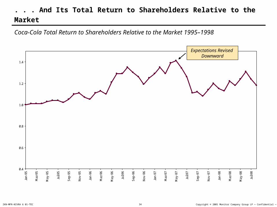
Analyst’s expectations of Coca Cola remained fairly constant during 1995 and 1996. However, falling expectations during 1997 and 1998 resulted in below market stock performance
1.0
1.1
1.2
1.3
1.4
1.5
1.6
1.7
1.8
1.9
2.0
Analyst Expectations of Coca-Cola EPS, 1995–1998: The Asian Crisis
Earnings per Share(adjusted for splits)
2 Years Ahead 1 Year Ahead
1 Year Ahead
2 Years Ahead 1 Year Ahead
1.18
1.41
1.67
1995 1996 1997 1998
Number of Analysts: 25 2527 22 22 20 20 19
Source: IBES, Monitor Analysis
1 Year Ahead
Expectations for Current Year (1 Year Ahead)Expectations for Next Year (2 Years Ahead)Actual Earnings Reported (Annual) 2 Years Ahead
Copyright © 2001 Monitor Company Group LP — Confidential — CAMZKN-MFR-NIVRA 6 01-TEC 34
0.4
0.6
0.8
1.0
1.2
1.4
Jan-
95
Mar
-95
May
-95
Jul-9
5
Sep
-95
Nov
-95
Jan-
96
Mar
-96
May
-96
Jul-9
6
Sep
-96
Nov
-96
Jan-
97
Mar
-97
May
-97
Jul-9
7
Sep
-97
Nov
-97
Jan-
98
Mar
-98
May
-98
Jul-9
8
Coca-Cola Total Return to Shareholders Relative to the Market 1995–1998
Expectations Revised Downward
. . . And Its Total Return to Shareholders Relative to the Market

Copyright © 2001 Monitor Company Group LP — Confidential — CAMZKN-MFR-NIVRA 6 01-TEC 35
Total Shareholder Return (TSR) Regression Results*
Traditional Performance Measures
Performance Measure Number of
Observations Adjusted R-
squared
Basic EPS (Scaled by Lagged Share Price) 2,522 4.5 %
Change in Basic EPS 2,522 5.1%
EVA (Scaled by Lagged Market Value) 2,182 0.3 %
Change in EVA 2,182 3.0 %
*The dependent variable for all regressions is market-adjusted TSR. Sample includes S&P 500 firms during 1992–98
Traditional performance metrics like EPS and EVA® are very poor predictors of returns to shareholders

Copyright © 2001 Monitor Company Group LP — Confidential — CAMZKN-MFR-NIVRA 6 01-TEC 36
Multiple Regression Results*
* S&P 500 firms during 1992–98. Sample has 2,390 observations
Variable Representing Changes in Analyst
Expectations
Regression Coefficients (T-Statistics in Parentheses)
Percent Change in Analyst Forecasts of Current Year's Earnings (EPS)
-0.01 (-0.34)
Percent Change in Analyst Forecasts of Next Year's Earnings (EPS)
0.70 (21.3)
Change in Analyst Forecasts of Long-Term (3–5 year) EPS Growth
8.6 (12.9)
Adjusted-R2 41.6%
Expectations about current earnings have no significant
impact on TSR
Expectations about current earnings have no significant
impact on TSR
Expectations about next year and long-term earnings have
significant impact on TSR
Expectations about next year and long-term earnings have
significant impact on TSR
Multiple regressions of market-adjusted total shareholder return (TSR) vs. changes in analyst earnings (EPS) expectations indicate a strong correlation between expectations and returns
Correlation is much higher than traditional metrics (EPS, EVA®)
Correlation is much higher than traditional metrics (EPS, EVA®)

Copyright © 2001 Monitor Company Group LP — Confidential — CAMZKN-MFR-NIVRA 6 01-TEC 37
Two Examples
Actual ROIC 200x WACC
Business A 30% 10%
Business B 5% 10%
Market Expected ROIC 200x
Management’s Revised Expectations 200x
Project X 40% 40%
Project Y 40% 20%
Which business unit did better?
Two projects are expected to earn 40% each and the cost of capital is 10%
Should we invest?

Copyright © 2001 Monitor Company Group LP — Confidential — CAMZKN-MFR-NIVRA 6 01-TEC 38
The Complete Picture
Value-Based Management:
Economic Profit = (ROIC-WACC) x Invested Capital
Expectations-Based Management:
EP = [Actual ROIC – Expected ROIC] x Invested Capital Work Core Assets Harder
– [Actual WACC – Expected WACC] x invested Capital Lower Cost of Capital
+ [ROIC – WACC] x [Actual IC – Expected IC] Invest Profitably

Copyright © 2001 Monitor Company Group LP — Confidential — CAMZKN-MFR-NIVRA 6 01-TEC 39
Integrated Framework for Expectations-Based Management
Operating Value Drivers, e.g.,
Cycle time
Customer retention rate
Churn rate
Non-performing loan rate
Operating Value Drivers, e.g.,
Cycle time
Customer retention rate
Churn rate
Non-performing loan rate
Actual vs. Expected
Annual Economic Profit
Actual vs. Expected
Annual Economic Profit
DCF ValueDCF ValueDrivesSummed
Over Time
Shareholder Value~~
Used by all levels of organization to set goals and measure
performance; used for benchmarking and sensitivity analysis
Measures short-term overall performance
by business
Value and compare strategies; measure long-term trade-offs
Together, DCF, EP, and value drivers form an integrated framework for value creation. DCF is comprehensive, long-term based, EP is a comprehensive, short-term measure, and value drivers are specific, short-term measures
EBM

Copyright © 2001 Monitor Company Group LP — Confidential — CAMZKN-MFR-NIVRA 6 01-TEC 40
Implications
Need to set expectations correctly with:
– Analysts, and shareholders
– Internal management team
Need to exceed expectations to have TRS exceed cost of equity
Take all new investments that are expected to have ROIC > WACC
Avoid the expectations treadmill with a two part incentive design
TRS = Cost of equity
+ Unexpected company performance
+ Unexpected market movements
Total Compensation = Salary + Bonus
Salaryt = f (Financial Performance in year t-1)
Bonust = f (Exceeding Expectations for year t )

Copyright © 2001 Monitor Company Group LP — Confidential — CAMZKN-MFR-NIVRA 6 01-TEC 41
Changes in Value are at the Heart of Economic Decision-Making
Discounted Cash Flow Valuation DCF
Expectations-Based Management
Real Options Analysis Real Options Analysis

Copyright © 2001 Monitor Company Group LP — Confidential — CAMZKN-MFR-NIVRA 6 01-TEC 42
Source: Dixit and Pindyck in Investment Under Uncertainty, Princeton University Press, 1994
Simple Investment Decision — Introduction
IllustrativeIllustrative
Facts:
Investment outlay = $1,600
Once made, the investment is irreversible
Replacement expense equals depreciation
Perpetual level cash inflows
Price level = $200 now
50 / 50 chance of price changing to $300 or $100 in one year
The price will stay at its new level forever
Cost of capital = 10%
200
(1.1)t
NPV = -1600 +
= -1600 + 2200
= 600
t=0
Consider the net present value approach to the following simple investment. When the expected cash flows are discounted at the cost of capital, the NPV is $600 and the decision is to invest. However . . .

Copyright © 2001 Monitor Company Group LP — Confidential — CAMZKN-MFR-NIVRA 6 01-TEC 43
. . . We have made an implicit assumption. We do not have to invest immediately, we can defer. If the project is deferred one year, it is possible to take advantage of price information. We would invest only if the price goes up. Regardless of whether it goes up or down, the NPV with deferral is $733 today
-1600
1.1NPV = .5
t=1
300
(1.1)t+ + .5
-1600
1.1
t=1
100
(1.1)t+
-1600 + 3300
1.1= .5 + .5
-1600 + 1100
1.1
= .5 + .5 [0]1700
1.1
= = $733850
1.1
Conclusion: Since the NPV of deferring is $133 higher than investing immediately, we would choose to defer, even though the NPV of investing immediately is large and positive
Do not invest if price falls to
$100
Do not invest if price falls to
$100
The Investment Decision as a Deferral Option

Copyright © 2001 Monitor Company Group LP — Confidential — CAMZKN-MFR-NIVRA 6 01-TEC 44
-1600
1.1NPV = .5
t=1
400
(1.1)t+ + .5
-1600
1.1
t=1
0
(1.1)t+
-1600 + 4400
1.1= .5 + .5
-1600 + 0
1.1
= .5 + .5 [0]2800
1.1
= = $1,2731400
1.1
Conclusion: The value of the deferral option goes up as there is greater uncertaintyPossible Macroeconomic Implication: Greater uncertainty in the economy (e.g., due to political unrest; uncertainty about taxes, interest rates or inflation) can cut investment because the deferral option becomes more valuable
Do not invest if price falls to $0Do not invest if price falls to $0
The value of deferral is a call option that is exercised when the irreversible investment is undertaken. The value of this option is affected by variance of prices (or costs), by the level of prices, by the scale of investment, by the level (and variance) of interest rates, and by the length of time that the deferral option lasts
Suppose the price in the previous example is equally likely to go to $400 or $0 (rather than $300 or $100)
The Value of a Deferral Option Increases with Variance
Copyright © 2001 Monitor Company Group LP — Confidential — CAMZKN-MFR-NIVRA 6 01-TEC 45
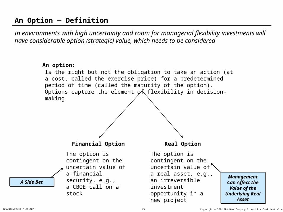
In environments with high uncertainty and room for managerial flexibility investments will have considerable option (strategic) value, which needs to be considered
An Option — Definition
Is the right but not the obligation to take an action (at a cost, called the exercise price) for a predetermined period of time (called the maturity of the option). Options capture the element of flexibility in decision-making
Financial Option
The option is contingent on the uncertain value of a financial security, e.g.,a CBOE call on a stock
Real Option
The option is contingent on the uncertain value of a real asset, e.g., an irreversible investment opportunity in a new project
An option:
Management Can Affect the Value of the
Underlying Real Asset
Management Can Affect the Value of the
Underlying Real Asset
A Side BetA Side Bet

Copyright © 2001 Monitor Company Group LP — Confidential — CAMZKN-MFR-NIVRA 6 01-TEC 46
Identifying Options — An Example of a Simple Option
Wrong Answer
NPV — No Flexibility
Wrong Answer
NPV — No Flexibility
Right Answer
Total Value with Flexibility
(ROA)
Right Answer
Total Value with Flexibility
(ROA)
The gray box is worthless because you can earn 10% by putting your money in the bank instead of earning 5% with the gray box (Problem: this assumes that the interest rate never changes)
The gray box is valuable because it is an option (you have the right, but not the obligation, to use it) and because interest rates are uncertain. There is a chance that the rate will fall below 5%. When it does, the option is valuable and will be exercised (the uncertainty in the interest rate is the key to understanding the problem)
NPV is misleading because it does not consider the option / flexibility value this box offers
$1.00
$1.05
Source: Steve Ross, Sterling Professor of Economics and Finance at Yale University
Consider a situation where you can put $1.00 into a gray box and get $1.05 back after a year with absolute certainty. Current interest rates are ten percent. How much is the gray box worth?

Copyright © 2001 Monitor Company Group LP — Confidential — CAMZKN-MFR-NIVRA 6 01-TEC 47
When is Managerial Flexibility Valuable?
Moderate Flexibility Value
HighFlexibility Value
HighFlexibility Value
Low Flexibility Value
Low Flexibility Value
ModerateFlexibility Value
ModerateFlexibility Value
High
Low
Low HighLikelihood of Receiving New InformationLikelihood of Receiving New Information
Uncertainty
Ro
om
fo
rM
an
ag
eri
al
Fle
xib
ilit
y
Ab
ilit
y t
o r
es
po
nd
Flexibility Value Greatest When:
1. High uncertainty about the future Very likely to receive new
information over time2. High room for managerial flexibility
Allows management to respond appropriately to this new information
1. High uncertainty about the future Very likely to receive new
information over time2. High room for managerial flexibility
Allows management to respond appropriately to this new information
+
3. NPV without flexibility near zero If a project is neither obviously
good nor obviously bad, flexibility to change course is more likely to be used and therefore is more valuable
3. NPV without flexibility near zero If a project is neither obviously
good nor obviously bad, flexibility to change course is more likely to be used and therefore is more valuable
Under these conditions, the difference between ROA and other decision tools is substantial
Under these conditions, the difference between ROA and other decision tools is substantial
In every scenario flexibility value is greatest when the project’s value without flexibility is close to break evenIn every scenario flexibility value is greatest when the project’s value without flexibility is close to break even
The flexibility value comes from the ability to respond to information that may be received in the future. The greater the likelihood that this new future information will elicit a managerial response and alter the course of a project, the more value the option will have

Copyright © 2001 Monitor Company Group LP — Confidential — CAMZKN-MFR-NIVRA 6 01-TEC 48
ToToToTo
Applicability — Progress to Date
The complication is that although real options are valuable, up to now option valuation has been an esoteric subject accessible only to those trained in stochastic calculus and other advanced mathematics. Recent advances in theory and technology, however, have allowed us to implement option pricing capability in simple algebraic formulas in Excel spreadsheets. Moreover, we can now handle more complicated situations when there are multiple sources of uncertainty that are not necessarily traded world commodities
FromFromFromFrom
Source of uncertainty not necessarily market priced
Algebra and Excel spreadsheets
Multiple sources of uncertainty(rainbow options)
Options on options (compound options, learning options)
Many applications
Source of uncertainty not necessarily market priced
Algebra and Excel spreadsheets
Multiple sources of uncertainty(rainbow options)
Options on options (compound options, learning options)
Many applications
Uncertainty driven by world commodity product
Higher mathematics necessary for application
Single source of uncertainty
Simple options
Limited application
Uncertainty driven by world commodity product
Higher mathematics necessary for application
Single source of uncertainty
Simple options
Limited application
Copyright © 2001 Monitor Company Group LP — Confidential — CAMZKN-MFR-NIVRA 6 01-TEC 49
American Call — Deferral Option
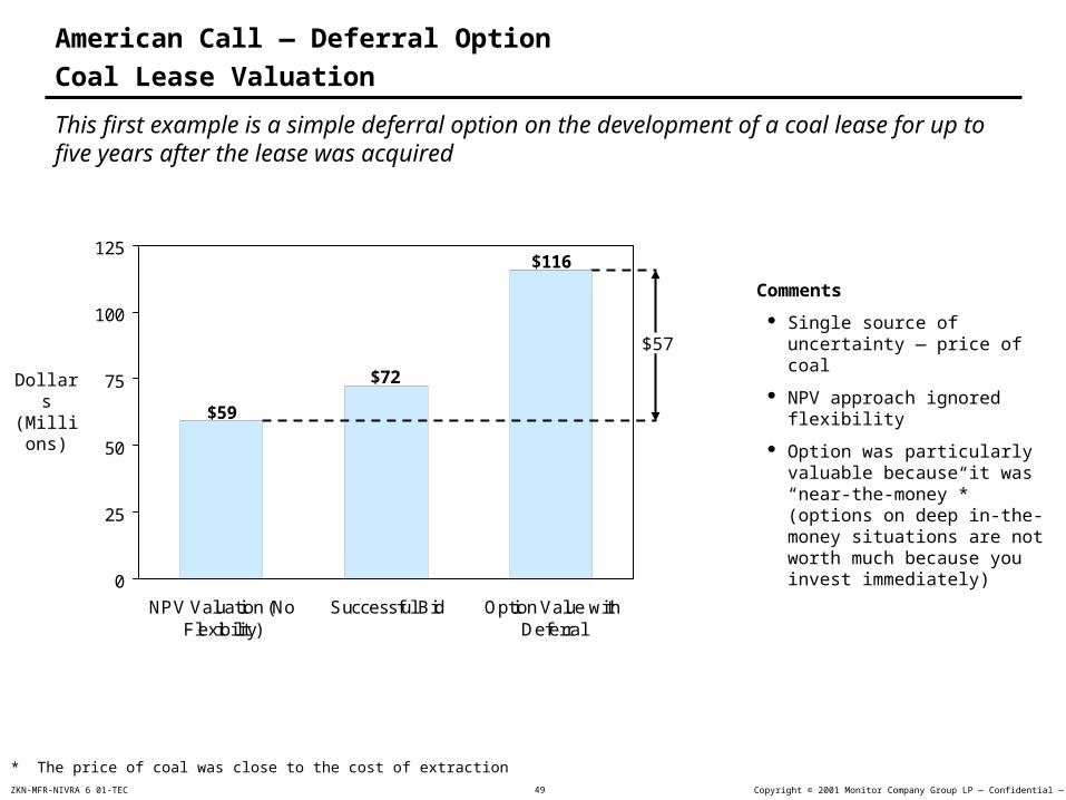
Coal Lease Valuation
This first example is a simple deferral option on the development of a coal lease for up to five years after the lease was acquired
Comments
Single source of uncertainty — price of coal
NPV approach ignored flexibility
Option was particularly valuable because it was “near-the-money”* (options on deep in-the-money situations are not worth much because you invest immediately)
$116
$72
$59
0
25
50
75
100
125
NPV Valuation (NoFlexibility)
Successful Bid Option Value withDeferral
Dollars (Millions)
$57
* The price of coal was close to the cost of extraction

Copyright © 2001 Monitor Company Group LP — Confidential — CAMZKN-MFR-NIVRA 6 01-TEC 50
It was possible to value cancelable operating leases because there is a relatively active market in second hand aircraft
Comments
Single source of uncertainty — price of second hand aircraft
Option value significantly underestimated by management
Leasing strategy changed
19%3%
16%
0%
5%
10%
15%
20%
25%
Pre-DeliveryPut Option
Walk-AwayOption
Total
Percent of Engine Price
83%25%
58%
0%
30%
60%
90%
Pre-DeliveryPut Option
Walk-AwayOption
Total
Wide-Body Aircraft Narrow Body Aircraft
American Put — Cancelable Operating Lease
The Value of Cancelable Operating Leases on Aircraft
Percent of Engine Price

Copyright © 2001 Monitor Company Group LP — Confidential — CAMZKN-MFR-NIVRA 6 01-TEC 51
Switching Option
The Value of Switching Options in Mining
Switching options apply to any situation where it is possible to shut down then reopen an operation
Comments
Study provided insight into when to open up and shut down operations
Single source of uncertainty
Value depended on the quantity of mineral in the ground, extraction costs, and the fixed cost of startup or shutdown, in addition to the usual list of variables
FlexibilityValue
Dollars (Millions)
$1,160
$710
$447
0
500
1,000
1,500
Initial NPV Estimate Scenario BasedNPV
Total

Copyright © 2001 Monitor Company Group LP — Confidential — CAMZKN-MFR-NIVRA 6 01-TEC 52
Despite the strong growth, consumer PC assembly players have found their market participation to be mostly dissatisfying as they are not earning their cost of capital
-2.3%
-1.5%
8.2%
11.0%
12.5%
-6.0%
-10% 0% 10% 20%
Consumer PCAssembly
Automobiles
ConsumerElectronics
Sports Shoes
Commercial IT
Beverages
Consumer Markets
Switching Option
Exit and Reentry Decision
Source: Analyst Reports; Annual Statements
-7.0%
-4.1%
-2.0%
29.7%
-11.0%
-20% 0% 20% 40%
Packard Bell
Apple
Compaq
Acer
Gateway
Consumer PC Assembly
Spread: ROIC–WACC Spread: ROIC–WACC

Copyright © 2001 Monitor Company Group LP — Confidential — CAMZKN-MFR-NIVRA 6 01-TEC 53
ROA Gives Different Decisions Than NPV and Economic Profit
Scenario ROV NPVEconomic Profit(WACC = 13.7%)
In Operation, Gross Margin = 13% Continue Continue Exit (ROIC = 7.6%)
In Operation, Gross Margin = 11% Continue Exit Exit (ROIC = 5.6%)
Not in Operation Don’t Enter Don’t Enter Don’t Enter (ROIC = 7.6%)
Traditional valuation techniques give mixed decisions about whether the unprofitable players should immediately exit the business. However, ROA suggests that players should stay in the market and exit only if conditions do not improve
Valuation Methodologies

Copyright © 2001 Monitor Company Group LP — Confidential — CAMZKN-MFR-NIVRA 6 01-TEC 54
ROA Gives Different Values* of Staying in Business than NPV and EP
Gross Operating Margin ROA
NPV + Flexibility Value
NPV (Cash Flows)
Economic Profit
(Short Term)
(ROIC–WACC) x IC
15% $2.98 $2.62 $0.05
13% $1.71 $1.02 -$0.07**
11% $0.79 -$0.59 -$0.09
9% $0.36 -$1.79 -$0.11
ROA gives significantly different value to the business than EP and NPV approaches (1997, $Billions)
Valuation Methodologies
* Assume a volatility of 16% annually for the gross operating margin (GOM)** ROIC before taxes = 7.6%, tax rate = 30%, WACC = 13.7%, invested capital is 26% of sales of $3.6 billion

Copyright © 2001 Monitor Company Group LP — Confidential — CAMZKN-MFR-NIVRA 6 01-TEC 55
Today (year 0), management does not need to commit to the entire project; it can simply begin the design process (at a cost of $50 million) and learn more about the operating spread uncertainty. Six months later, management has a similar option, to begin the pre-construction process without a full commitment and learn more about the uncertainties. At the end of the year, management no longer has the flexibility to learn more about the uncertainty and must choose between a full commitment or abandonment
Year 0 Six Months End of Year 1
Decision Node
Invest $50 million for design process only
Invest $50 million for design process only
Full commitment — no flexibility Full commitment — no flexibility
Abandon — no flexibility Abandon — no flexibility
Invest $200 million only to start pre-construction work
Invest $200 million only to start pre-construction work
Full commitment — no flexibility Full commitment — no flexibility
Abandon — no flexibility Abandon — no flexibility
Full commitment — invest $400 million
Full commitment — invest $400 million
Abandon Abandon
Uncertainty evolves but we cannot react
Eliminated managerial flexibility, and therefore destroyed option value
Uncertainty evolves but we cannot react
Eliminated managerial flexibility, and therefore destroyed option value
Compound Option — Multiphase investment
The Value of Compound Options in Plant Construction

Copyright © 2001 Monitor Company Group LP — Confidential — CAMZKN-MFR-NIVRA 6 01-TEC 56
The Source of Uncertainty
0
200
400
600
800
1,000
1,200
1,400
1Q79 4Q79 2Q81 1Q81 1Q82 3Q83 2Q84 1Q85 4Q85 3Q86 2Q87 1Q88 4Q88 3Q89 2Q90 1Q91 4Q91 3Q92 2Q93 1Q94 4Q94 3Q95 2Q96 4Q96
Operating Spread = Output Price / Ton – Input
At first there seems to be two sources of uncertainty: the price of the output per ton, and the cost of the input per ton. However, these can be combined into a single source of uncertainty, the operating spread
Estimated Data Estimated Data
Output Price
Input Price
Price History — First Quarter 1979 to Fourth Quarter 1996

Copyright © 2001 Monitor Company Group LP — Confidential — CAMZKN-MFR-NIVRA 6 01-TEC 57
Summary — Phased Investment
$ Millions
The traditional NPV approach dramatically undervalues this investment since it does not consider the value of flexibility. Since this is a multi-staged investment, management has the flexibility to re-evaluate the project at each stage and refine their strategy based on new information. A full commitment (to either accept or abandon) eliminates managerial flexibility and destroys the option (flexibility) value
- $71.2
$354.5 $425.7
NPV Valuation: No Flexibility
Flexibility Value Total Value (ROA)

Copyright © 2001 Monitor Company Group LP — Confidential — CAMZKN-MFR-NIVRA 6 01-TEC 58
Planned
Abandon
Planned + 50%
Planned
Abandon
The decision tree below shows a stylized version of the decision to develop a large energy resource. There were two sources of uncertainty, the price of energy and the amount of resource in the ground, and there were compound options
Illustrative
* Simplified for illustrative purposes** Capacity planned before ROA analysis
11
11
11
11
11
11
Assumed decision nodes
Initial capacity decision
Year 3 initial capacity decision
Year 11 capacity addition decision
Exploration decision
Event nodes (uncertain outcomes) Prices go up or down? Reserves in existing fields are
higher or lower than EV? Resource quantity found in 4 add-
on fields worth developing or not?
1
3
11
E
OPM Cases
Capacity “lock-in”
Defer capacity decision and exploration
Defer capacity decision / explore today
1
2
3
Planned capacity 50% of planned capacity Abandon
Planned capacity 50% of planned capacity Abandon
11
11
11
1
Planned capacity** plus 50%
Planned capacity*
Abandon
Planned capacity** + 50%
Planned
Abandon
Planned + 50% 11
11
11
E
$ High
2
2
2
$ Low
Explore
E How much to invest in exploration during Year 1 through Year 3?
What capacity to lock-in in Year 3?
Do not explore in the near term
95
What capacity level to lock into today?
Lock in capacity now
1
3
Defer capacity decision
Explore in the interim? (Year 1-Year 3)
Lock in capacity today or defer decision until Year 3?
Add capacity in Year 11?
2
Compound Rainbow Option
Exploration and Development

Copyright © 2001 Monitor Company Group LP — Confidential — CAMZKN-MFR-NIVRA 6 01-TEC 59
OPM Case
A. Initial Capacity
Decision
B. Exploration
Decision
C. Add-on Capacity
Decision
No-options base case †
Capacity "lock-in"
Year 6
Defer capacity decision and exploration
Year 3 Year 6
Defer capacity decision / explore today
Year 3
ROA Model Valuation Results*
The optimal solution provided more than twice the value and was completely different from the client’s base case
225
200
150
100
0 100 200
Total Project Value Estimates**
Normalized Currency Units
* Throughout the document the results have been normalized and rounded off to provide general insights while maintaining client confidentiality** For comparison purposes and because of lack of information, each of the 4 cases assume a Year 1 exploration cost equal to 0; if “best-guess” exploration
cost of estimates of 40 is used, the NPV for the 3 option cases are 120, 175, and 185, respectively† Analogous to traditional DCF case (i.e., assumes deterministic inputs and no managerial flexibility)
11
22
33
+Value of reserve size information
Value of price information
Value of Better capacity
lock in decision Exploration option Expansion option
Today (planned capacity)
Today(No exploration)
Today(No exploration)
Today (planned capacity +50%)
TodayExplore
Most attractive operating plan
Year 11
Year 11
Year 11

Copyright © 2001 Monitor Company Group LP — Confidential — CAMZKN-MFR-NIVRA 6 01-TEC 60
Classic Questions and Their Answers
1. Option values are contingent on the current value and the expected volatility of the underlying security or asset. If one holds a call option on a share of stock, the market price is observable and we can estimate the expected volatility. But a real option is contingent on an asset that is not traded in a capital market (e.g., a cure for baldness). What do we do?Marketed Asset Disclaimer (MAD): We assume that the present value of the asset without flexibility is the same as the market price for which the underlying asset (without flexibility) can be bought or sold
2. Lattices (Binomial tress in particular) are a discrete approach to modeling the Gauss-Wiener continuous scholastic process that Black-Scholes assumed for the underlying security when they derived the closed-form solution For European call options. But, project cash flows do not follow, or even roughly approximate a “regularized” binomial latticeProperly Anticipated Process Fluctuate Randomly (PAP): Paul Samuelson proved that the bid of any pattern of the future cash flows contains all expectations and therefore moves randomly through time (obeying a Gauss-Wiener Process), deviating only with unexpected changes in the problem of cash flows

Copyright © 2001 Monitor Company Group LP — Confidential — CAMZKN-MFR-NIVRA 6 01-TEC 61
-20-10
2010
3020
1020
40
A Four-Step Process
Free Cash Flows
PV Free CashFlow
Year
0 1 2 3 4 5 6 7 8
PV
Value
Year
Cash In
Cash Out
Free Cash Flows1 2 . . . . . . 10 CV
Price
Quantity
Variable Cost
Interest Rates
The Year Spread Sheet
Evolution of Project Value
Value (t = 1) n (V1 / V0) = r
Monte CarloSimulation
V0
uV
dV
u2V
duV
d2V
u3V
u2dV
d2uV
d3V
Event Tree(Sans
Dividends)
Step One
Complete the base case present value (without flexibility) based on
– Expected future free cash flows– Cost of capital based on
comparables
Step Two Estimate the volatility of the value of
the project in order to derive the volatility of the rate of return
– A Monte Carlo approach can combine many uncertainties
– The volatility of the drivers of uncertainty may be estimated from internal data or from subjective estimates made by management
The output is a binomial lattice in value
Note that the expected value of the project evolves through time as shown in the figure to the right
udeu /1, T
WACC = 10%

Copyright © 2001 Monitor Company Group LP — Confidential — CAMZKN-MFR-NIVRA 6 01-TEC 62
Four Step Process (cont.)
Go, StopGo, Stop
Expand, AbandonExpand, Abandon
Expand, AbandonExpand, Abandon
Expand, ContractExpand, Contract
Expand, ContractExpand, Contract
Expand, AbandonExpand, Abandon
ROA0
Go
ROA2
Expand
ROA1
Abandon ROA2
Abandon
ROA1
GoROA2
Go
Step Three
Put decisions into the nodes of the event tree
– Can have multiple decisions per node
– Payouts may include cash flows as dividends
Step Four
Work backward in the tree (unless there is path dependency) to obtain values at each node and to make optimal decisions
– Use no arbitrage condition to conform to law of “one price”
– Output is the value of the project with flexibility and decision rules

Copyright © 2001 Monitor Company Group LP — Confidential — CAMZKN-MFR-NIVRA 6 01-TEC 63
Project Analysis
Overall Approach — A Four Step Process
Objectives
Comments
Compute base case present value without flexibility at t = 0
Value the total project using a simple algebraic methodology
Identify major uncertainties in each stage
Understand how those uncertainties affect the PV
Analyze the event tree to identify and incorporate managerial flexibility to respond to new information
Still no flexibility; this value should equal the value from Step 1
Explicitly estimate uncertainty
Incorporating flexibility transforms event trees, which transforms them into decision trees
The flexibility continuously alters the risk characteristics of the project, and hence the cost of capital
ROA includes the base case present value without flexibility plus the option (flexibility) value
– Under high uncertainty and managerial flexibility option value will be substantial
Steps
Output Project’s PV without flexibility
Detailed event tree capturing the possible present values of the project
A detailed scenario tree combining possible events and management responses
ROA of the project and optimal contingent plan for the available real options
Model theUncertainty
Using Event Trees
Identify and Incorporate Managerial
Flexibilities Creating a Decision Tree
Calculate Real Option Value (ROA)
Compute Base CasePresent Value withoutFlexibility Using DCF
Valuation Model

Copyright © 2001 Monitor Company Group LP — Confidential — CAMZKN-MFR-NIVRA 6 01-TEC 64
Step 4 — Valuation Using the “No Arbitrage” Condition
Using the traded twin security we can value our project in year 0 using either the traditional cost of capital approach, or the replicating portfolio method. Under the cost of capital approach we calculate the expected rate of return using the twin and then discount the cash flows from our project at this rate*. Alternatively, we can calculate how many shares (N) of the twin security would replicate the cash flow of our project** in any state, and calculate the value of those shares in year 0 (N shares x price / share). These two methods will yield the same result since the cost of capital approach is essentially a shortcut for the replicating portfolio method***
*Since the “twin security” is a traded security with the same risk characteristics as our project (by definition), its required rate of return (discount rate) must be equal to the discount rate on our project. CAPM simply generalizes this by claiming all securities with the same Beta (systematic risk) will have the same cost of capital (if all equity financing); therefore, identifying a security’s Beta is equivalent to finding a priced “twin security”**Typically the replicating portfolio will be a leveraged position that will also entail borrowing***Since the project and this portfolio provide the same future returns, to avoid risk-free arbitrage they must have the same value in year 0
Year 0
Twin Security
Our Project
P0 = 20 V0 = ?
Year 1
Twin Security
Our Project
$34 $170
Twin Security
Our Project
$13 $65
Probabilit
y = 50%
Probability = 50%
Calculating V0
Method 1:Cost of Capital Approach
Method 2:Replicating Portfolio**
1. Calculate cost of capital using “twin security”
20 = (0.5)(34)+(0.5)(13)1+k
k = 17.5%
2. Discount expected cash flows
V0 = (0.5)(170)+(0.5)(65)1.175
V0 = 100
1. Replicating cash flows of our security using a portfolio of “twin” and borrowing in year 1
34N + B = 170 13N + B = 65 N = 5; B = 0
2. Value of this portfolio in year 0
V0 = 20N + B V0 = 100

Copyright © 2001 Monitor Company Group LP — Confidential — CAMZKN-MFR-NIVRA 6 01-TEC 65
NPV / DCF Valuation — Flexibility Not Valued
* [(0.5) (170) + (0.5) (65)] / 1.175 = 100** 115 / 1.08 = 106.48: The investment is discounted at the risk-free rate because the decision to invest was made in Year 0
Using the NPV / DCF methodology, this project would be rejected since it has a negative NPV of -$6.5
100
-106.5
-6.5
Present Value ofCash Flows*
Present Value ofInvestments**
NPV
Decision Made in Year 0
Decision Made in Year 0
Probability = 50%
Probability = 50%
Cash Flows
170
65
Investment
-115
-115
Value in Year 0 Decision
Do NotInvest
Since the decision to invest was made in Year 0,
we are bound into a negative NPV project in the
unfavorable state
Since the decision to invest was made in Year 0,
we are bound into a negative NPV project in the
unfavorable state
Year 0 Year 1

Copyright © 2001 Monitor Company Group LP — Confidential — CAMZKN-MFR-NIVRA 6 01-TEC 66
Real Option Analysis — Flexibility Valued (cont.)
* To see derivation of this column see Decision Tree Analysis chart** See NPV / DCF valuation† Total value less NPV; this could be valued separately†† 2.62 shares X $20 / share -$31.43 = $20.95
27.4
-6.5
20.9
NPV** FlexibilityValue
Total Value
Decision Deferred
Until Year 1
Decision Deferred
Until Year 1
Probability = 50%
Probability = 50%
55
0
Invest;Based onFlexibility
Value
Value of N shares @ $34 / share
Value of loan (B) 34N+B(1+rf)=55
Value of N shares @ $13 / Share
Value of loan(B) 13N+B(1+rf )=0
Net CFs*
CFs Replicated UsingN Shares of “Twin
Security” and Borrowing
Replicating Portfolio in
Year 0
† ††
Year 0 Year 1
The ROA approach values the total project, with flexibility, at $20.95 ($2.54 less than the DTA value). Since the ROA method is calculated using replicating portfolios, this must be the correct value — otherwise there would be arbitrage opportunities
Value in Year 0 Decision
Buy 2.62 shares @ $20 / share
Borrow $31.43
Value = 20.95††

Copyright © 2001 Monitor Company Group LP — Confidential — CAMZKN-MFR-NIVRA 6 01-TEC 67
Real Option Analysis — Flexibility Valued
* To see derivation of this column see Decision Tree Analysis chart** See NPV / DCF valuation† Total value less NPV; this could be valued separately†† 0.52 shares X $100 / share -$31.42 = $20.95
27.4
-6.5
20.9
NPV** FlexibilityValue
Total Value
Decision Deferred
Until Year 1
Probability = 50%
Probability = 50%
55
0
Invest;Based onFlexibility
Value
Value of N shares @ $170 share
Value of loan (B) 170N+B(1+rf)=55
Value of N shares @ $65 / Share
Value of loan(B) 65N+B(1+rf )=0
Net CFs*
CFs Replicated UsingN Shares of “PV Type”
(without flexibility) and Borrowing
Replicating Portfolio in
Year 0
† ††
Year 0 Year 1
Rather than searching for a fictitious “twin security” we use the present value of the project itself, without flexibility, as the underlying risky asset. What is better correlated with the project that the project itself? We call this the Marketed Asset Disclaimer (MAD)
Value in Year 0 Decision
Buy 0.524 shares @ $100 / share
Borrow $31.53
Value = 20.95††

Copyright © 2001 Monitor Company Group LP — Confidential — CAMZKN-MFR-NIVRA 6 01-TEC 68
Marketed Asset Disclaimer Assumption
Both the replicating portfolio approach and the risk-adjusted method (as we will apply them in this section) rely heavily on the Marketed Asset Disclaimer assumption
Both the replicated portfolio approach and the risk-adjusted method rely on our ability to buy shares of the base case present value (without flexibility) when creating the replicating portfolios. If the present value is traded (as in the case of a stock) this will not be a problem; however when the present value is not explicitly traded (as will usually be the case with real options) our ability to build the replicating portfolio becomes dubious
The Marketed Asset Disclaimer assumption implies that we assume that even if the base case present value is not marketed we can still build the replicating portfolios, because if it were marketed, the value we calculated (with our DCF model) would be approximately equal to the publicly traded market value (if it existed); therefore the replicating portfolio approach (and equivalently the risk-adjusted method) would still produce the correct value
There are other approaches in the academic literature, however, noted academics Steve Ross and Eduardo Schwartz support the Marketed Asset Disclaimer method

Copyright © 2001 Monitor Company Group LP — Confidential — CAMZKN-MFR-NIVRA 6 01-TEC 69
20.9 = (0.5)(55)+(0.5)(0)
1+k
k = 31.9%
The original cost of capital was 17.5%
20.9 = (0.5)(55)+(0.5)(0)
1+k
k = 31.9%
The original cost of capital was 17.5%
The Correct Cost of Capital
The cost of capital, as calculated from correct ROA value is 31.9%. Since this differs from the original cost of capital for the project without flexibility (17.5%), flexibility has therefore altered the project’s riskiness
* To see derivation this column see Decision Tree Analysis chart
Net CFs*
55
0
Probabilit
y = 50%
Probability = 50%
Cost of Capital Year 0 Year 1
Value20.9
Value20.9

Copyright © 2001 Monitor Company Group LP — Confidential — CAMZKN-MFR-NIVRA 6 01-TEC 70
Step 3 — Decision Trees
Initial Conditions (No Flexibility) — Event Tree for Underlying Asset
Assumptions Risk-free rate of 5% WACC of 12% Initial investment of $105MM Five year time frame (analyzing one period
per year)
Underlying Asset A factory with a (no flexibility) present value of
$100MM The standard deviation of the rate of change of the
factory value (volatility) is 15%No Flexibility (NPV)
($5MM) = $100MM – $105MM
212182
157 157135 135
116 116 116100 100 100
86 86 8674 74
64 6455
47
t=0 t=1 t=2 t=3 t=4 t=5
Value =
– Investment = -105
-5NPV
Value-basedEvent Tree
Value-basedEvent Tree

Copyright © 2001 Monitor Company Group LP — Confidential — CAMZKN-MFR-NIVRA 6 01-TEC 71
Step 3: Real Options Calculations Examples
Option to Expand
Management has the right to expand the scale and the value of the factory by 20% at any point in time by investing an additional $15MM
239204
175 173149 148
127 126 124108 107 106
91 90 8877 75
65 6455
47
t=0 t=1 t=2 t=3 t=4 t=5
Underlying Asset ValuesPV+ = 86PV- = 64PV = 74
Managerial Decisions (t=4,5)88 = Max (86, 86*1.2-15)64 = Max (64, 64*1.2-15)75 = Max (75, 74*1.2-15)
Portfolio Replicationn = (88 - 64) / (86 - 64)B = [88 - n (86) ] / (1+5%)n = 1.1, B = -5.54
Value of Option (ROA at t=4)ROA = n (74) + BROA = 75
Underlying Asset ValuesPV+ = 86PV- = 64PV = 74
Managerial Decisions (t=4,5)88 = Max (86, 86*1.2-15)64 = Max (64, 64*1.2-15)75 = Max (75, 74*1.2-15)
Portfolio Replicationn = (88 - 64) / (86 - 64)B = [88 - n (86) ] / (1+5%)n = 1.1, B = -5.54
Value of Option (ROA at t=4)ROA = n (74) + BROA = 75
Note: In this case management will never exercise its option prior to the five year expiration date. In general, a call option on a non-dividend paying asset will never be exercised early
= Decision to Expand
Copyright © 2001 Monitor Company Group LP — Confidential — CAMZKN-MFR-NIVRA 6 01-TEC 72
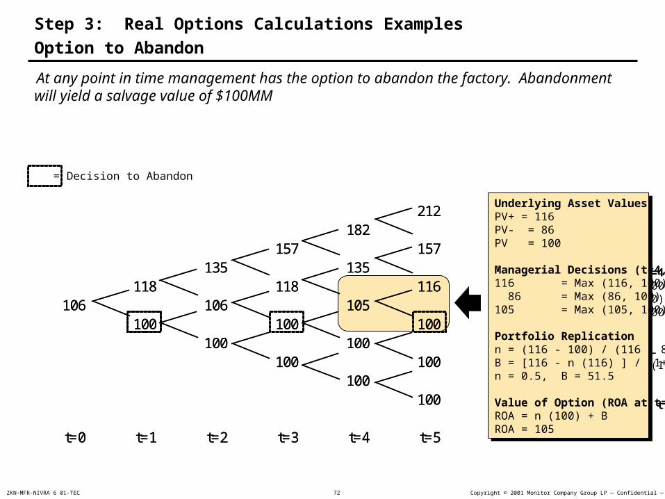
Step 3: Real Options Calculations Examples
Option to Abandon
At any point in time management has the option to abandon the factory. Abandonment will yield a salvage value of $100MM
212182
157 157135 135
118 118 116106 106 105
100 100 100100 100
100 100100
100
t=0 t=1 t=2 t=3 t=4 t=5
Underlying Asset ValuesPV+ = 116PV- = 86PV = 100
Managerial Decisions (t=4,5)116 = Max (116, 100) 86 = Max (86, 100)105 = Max (105, 100)
Portfolio Replicationn = (116 - 100) / (116 - 86)B = [116 - n (116) ] / (1+5%)n = 0.5, B = 51.5
Value of Option (ROA at t=4)ROA = n (100) + BROA = 105
Underlying Asset ValuesPV+ = 116PV- = 86PV = 100
Managerial Decisions (t=4,5)116 = Max (116, 100) 86 = Max (86, 100)105 = Max (105, 100)
Portfolio Replicationn = (116 - 100) / (116 - 86)B = [116 - n (116) ] / (1+5%)n = 0.5, B = 51.5
Value of Option (ROA at t=4)ROA = n (100) + BROA = 105
= Decision to Abandon
212182
157 157135 135
118 118 116106 106 105
100 100 100100 100
100 100100
100
t=0 t=1 t=2 t=3 t=4 t=5

Copyright © 2001 Monitor Company Group LP — Confidential — CAMZKN-MFR-NIVRA 6 01-TEC 73
Step 3: Real Options Calculations Examples
Option to Contract
At any point in time management has the option to decrease the scale and the value of the factory by 25%, generating savings of $25MM
212182
157 157135 135
117 117 116102 101 101
90 90 9081 81
73 7366
60
t=0 t=1 t=2 t=3 t=4 t=5
Underlying Asset ValuesPV+ = 116PV- = 86PV = 100
Managerial Decisions (t=4,5)116 = Max (116, 116*0.75+25)90 = Max (86, 86*0.75+25)101 = Max (101, 100*0.75+25)
Portfolio Replicationn = (116 - 90) / (116 - 86)B = [116 - n (116) ] / (1+5%)n = 0.87, B = 14.4
Value of Option (ROA at t=4)ROA = n (100) + BROA = 101
= Decision to Contract
Copyright © 2001 Monitor Company Group LP — Confidential — CAMZKN-MFR-NIVRA 6 01-TEC 74
239204
175 173150 148
129 127 124113 112 110
102 101 100100 100
100 100100
100
t=0 t=1 t=2 t=3 t=4 t=5
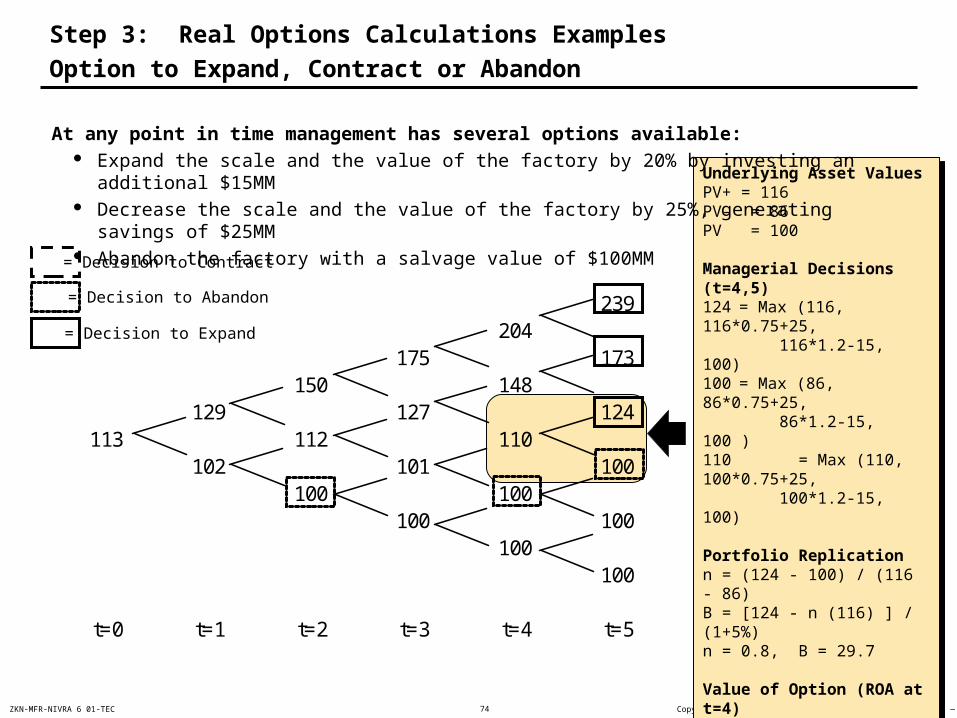
Underlying Asset ValuesPV+ = 116PV- = 86PV = 100
Managerial Decisions (t=4,5)124 = Max (116, 116*0.75+25,
116*1.2-15, 100)100 = Max (86, 86*0.75+25,
86*1.2-15, 100 )110 = Max (110, 100*0.75+25,
100*1.2-15, 100)
Portfolio Replicationn = (124 - 100) / (116 - 86)B = [124 - n (116) ] / (1+5%)n = 0.8, B = 29.7
Value of Option (ROA at t=4)ROA = n (100) + BROA = 110
= Decision to Contract
= Decision to Abandon
= Decision to Expand
Step 3: Real Options Calculations Examples
Option to Expand, Contract or Abandon
At any point in time management has several options available: Expand the scale and the value of the factory by 20% by investing an additional $15MM Decrease the scale and the value of the factory by 25%, generating savings of $25MM Abandon the factory with a salvage value of $100MM

Copyright © 2001 Monitor Company Group LP — Confidential — CAMZKN-MFR-NIVRA 6 01-TEC 75
For the time being, assume that the uncertainties all move continuously through time and remember that the annualized volatility (we need to calculate is the volatility of the percent value which is usually hard to observe. Several factors combine to convert the uncertainty of the real market prices, quantities, and costs that feed into the company to the equity uncertainty that is manifested in the financial markets
PricePrice
QuantityQuantity
CostCost
PricePrice
QuantityQuantity
CostCost
Op
era
ting
Le
ve
rag
e
Div
ers
ifica
tion
Fin
an
cia
l Le
ve
rag
e
RealMarkets
Data
Project Uncertainties Asset Uncertainties
Equity Uncertainty
FinancialMarkets
Data
Not directly observable
Step 2 — Modeling Uncertainties and Building the Event Tree

Copyright © 2001 Monitor Company Group LP — Confidential — CAMZKN-MFR-NIVRA 6 01-TEC 76
The base-case present value without flexibility for the investment is estimated a thousand times to generate the standard deviation of the rate of return
Valuation Model DCF
Net present value for the investment
Net present value for the investment
Valuation Inputs Revenue growth rates Margin assumptions Capital expenditures
Ud
eU T
1
Monte Carlo
Random NumberRandom Number GeneratorGenerator
Random NumberRandom Number GeneratorGenerator
rV
Vn
0
1
based on r

Copyright © 2001 Monitor Company Group LP — Confidential — CAMZKN-MFR-NIVRA 6 01-TEC 77
Calculating Volatility Direct From Historic Market Data
If we have historical market data we can calculate the volatility of present value directly
Transform into Natural Logs
Calculate Variance
Compute Growth Rate
Jan ‘89:
Annualize
vart
Convert into Volatility (v)
SQRT (VAR) ( )
Date Value
Growth Rate LN (Growth Rate) Variance Volatility Annualize
Example:
Comments:
Feb ‘89:
Mar ‘89:
April ‘89:
2
4
3
5
G1=4/2
G2=3/4
G3=5/3
Ln4-ln2= .69
Ln3-ln4= -.29
Ln5-ln3= .51
.27 .271/12
= 3.26 SQRT (3.26) = 1.81
t is based on the time series data; in this example t = 1/12 since the data is monthly
Once we know the annualized volatility, we can use a different t in the building the tree
Get Time Series Data

Copyright © 2001 Monitor Company Group LP — Confidential — CAMZKN-MFR-NIVRA 6 01-TEC 78
Calculating Volatility from Management Estimates
What is the 95% confidence level in year 5?
$
100
20
o
ro
o
lower
i
P
Pn
lr
ePP
Pp
r
6
6
2
Expected

Copyright © 2001 Monitor Company Group LP — Confidential — CAMZKN-MFR-NIVRA 6 01-TEC 79
Keeping Uncertainties Separate
When technological uncertainty evolves discontinuously and other uncertainties evolve continuously, we use a quadrarial approach
Tech Good
Tech Bad
Tech Good
Tech Bad
Tech Average
Market UpMarket Down
Market Up
Market Down
Market Up
Market Down
Market Up
Market Down
Market Up
Market Down

Copyright © 2001 Monitor Company Group LP — Confidential — CAMZKN-MFR-NIVRA 6 01-TEC 80
Portes Case — Situation
1. Portes founded 10 years ago, 60 employees, CEO Diane Mullins
2. Slow growth of profitable systems recovery product, Recovery™
3. New high-end data recovery software — can be sold over the Internet
4. Bill, the CFO, finds that selling in France — The Portes Project — via the Internet, has a negative NPV. Monte Carlo analysis doesn’t help [see table 1 for the analysis]
Sales of 200 programs in year 1, doubles to 400 in 5 years Unit price starts at $30,000 and falls to $20,000 in 5 years COGS is $9,000 per program in year 1 and falls to $7,000 in 6th year Fixed cost $20,000 per year SG&A? is 10% of revenue Initial investment is $35 million, depreciated over 10 years No debt 40% tax rate 13% cost of capital Beyond year 10, FCF grows at 4%, and ROIC 12%
5. Risk estimates, in 6th year Unit sales, expected level is 400 programs and the lower 95% confidence limit is 190 Unit price, expected level is $20,000 and the lower 95% confidence limit is $25,000
6. Flexibility in decision-making Expansion (prevent loss product), invest $10.5 million and increase value 30% Abandonment value is $15 million

Copyright © 2001 Monitor Company Group LP — Confidential — CAMZKN-MFR-NIVRA 6 01-TEC 81
Table 1
NPV Analysis of the Investment Proposal
Item Year 0 Year 1 Year 2 Year 3 Year 4 Year 5 Year 6 Year 7
Quantity (units) 200 230 264 303 348 400Continuous Annual Growth Rate 13.9%
Price per unit 30.00 27.66 25.51 23.52 21.69 20.00Continuous Annual Growth Rate -8.1%
Cost per unit 9.0 8.6 8.1 7.7 7.4 7.0
Revenues 6,000 6,355 6,732 7,130 7,553 8,000Cost of Goods Sold 1,800 1,966 2,148 2,346 2,563 2,800
Gross Income 4,200 4,389 4,584 4,784 4,990 5,200Gross Margin% 70% 69% 68% 67% 66% 65%
Rent 200 200 200 200 200 200S&A expenses 600 636 673 713 755 800
EBITDA 3,400 3,554 3,711 3,871 4,034 4,200
Depreciation 3,500 3,500 3,500 3,500 3,500 3,500
EBIT (100) 54 211 371 534 700EBIT Growth -154% 294% 76% 44% 31%
Taxes 0 21 84 148 214 280
Net Income (100) 32 126 223 321 420
Depreciation 3,500 3,500 3,500 3,500 3,500 3,500
Initial Investment 35,000
Free Cash Flow (35,000) 3,400 3,532 3,626 3,723 3,821 3,920Change in FCF 4% 3% 3% 3% 3%
Continuous Value 50,960
Discount Rate 13%
PV 34,681 36,096 37,575 39,165 40,880 42,735 44,748TPV (319) 39,496 41,107 42,792 44,603 46,555 48,668FCF as a % of PV 8.6% 8.6% 8.5% 8.3% 8.2% 8.05%
Copyright © 2001 Monitor Company Group LP — Confidential — CAMZKN-MFR-NIVRA 6 01-TEC 82
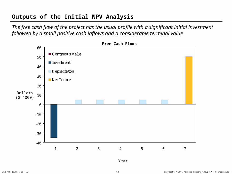
Outputs of the Initial NPV Analysis
The free cash flow of the project has the usual profile with a significant initial investment followed by a small positive cash inflows and a considerable terminal value
Free Cash Flows
Dollars($ ‘000)
-40
-30
-20
-10
0
10
20
30
40
50
60
1 2 3 4 5 6 7
Continuous Value
Investment
Depreciation
Net Income
Year
Copyright © 2001 Monitor Company Group LP — Confidential — CAMZKN-MFR-NIVRA 6 01-TEC 83
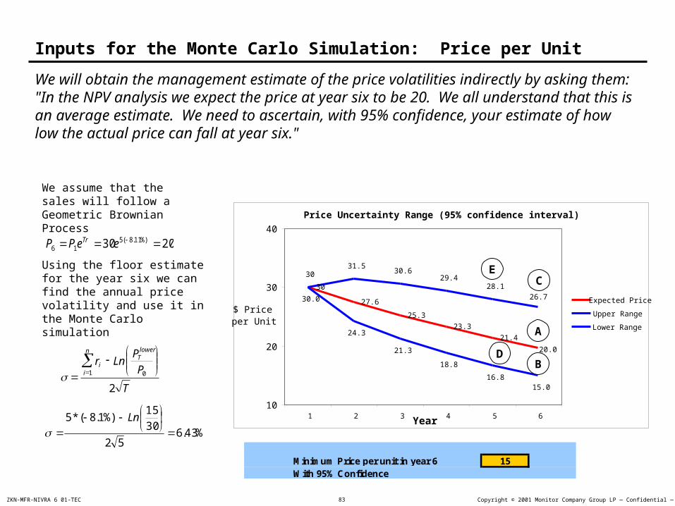
Inputs for the Monte Carlo Simulation: Price per Unit
Price Uncertainty Range (95% confidence interval)
30
27.6
25.3
23.3
21.4
20.0
3031.5
30.629.4
28.1
30.0
24.3
21.3
18.8
16.815.0
26.7
10
20
30
40
1 2 3 4 5 6Year
$ Price per Unit
Expected Price
Upper Range
Lower Range
Minimum Price per unit in year 6 15With 95% Confidence
EC
A
DB
We will obtain the management estimate of the price volatilities indirectly by asking them: "In the NPV analysis we expect the price at year six to be 20. We all understand that this is an average estimate. We need to ascertain, with 95% confidence, your estimate of how low the actual price can fall at year six."
T
P
PLnr
lowerT
n
ii
2
01
We assume that the sales will follow a Geometric Brownian Process
Using the floor estimate for the year six we can find the annual price volatility and use it in the Monte Carlo simulation
2030 %)11.8(516 eePP Tr
%43.652
30
15%)1.8(*5
Ln

Copyright © 2001 Monitor Company Group LP — Confidential — CAMZKN-MFR-NIVRA 6 01-TEC 84
Inputs for the Monte Carlo Simulation: Units Sold
Units Sold: Uncertainty Range (95% confidence interval)
200229 264
300348
400200
320.5
422.6
539.6
677.7
200164.7 164.8 170.3 178.9 190.0
842.1
0
100
200
300
400
500
600
700
800
900
1 2 3 4 5 6Year
Number of Units
Expected Quantity
Up Range
Low Range
Minimum Sales Quantity in year 6 190With 95% Confidence
EC
A
BD
To obtain management's estimate of the sale quantity volatility we ask a similar question: "Given that the expected average sales for year six is 400, what is the level where we can expect with 95% confidence that the actual sales will be higher?"
T
P
PLnr
lowerT
n
ii
2
01
400200 86.13*516 eeQQ Tr
We assume that the sales will follow a Geometric Brownian Process
Using the floor estimate for the year six we can find the annual sales volatility and use it in the Monte Carlo simulation
65.1652
200
19086.13*5
Ln

Copyright © 2001 Monitor Company Group LP — Confidential — CAMZKN-MFR-NIVRA 6 01-TEC 85
Output of the Monte Carlo Simulation: Volatility of the Project’s Value
Frequency Chart
.000
.009
.018
.026
.035
0
8.75
17.5
26.25
35
-75% -31% 13% 56% 100%
1,000 Trials 4 Outliers
Forecast: Expected Annual Return
Now we can complete the whole Monte Carlo simulation, and run the uncertainties through the NPV model to get an estimate for the volatility of the project's value.
For 1000 trials the distribution of the rate of return approximates normal distribution with a mean value of 12%. The volatility (standard deviation) of the rate of return is 30%

Copyright © 2001 Monitor Company Group LP — Confidential — CAMZKN-MFR-NIVRA 6 01-TEC 86
Event Tree for the Present Value of the Project Without Flexibility
Having combined management estimates of uncertainty about price and quantity into a single uncertainty of the value of the project, we can build a value-based event tree.
Adding back the initial $35 million investment yields the present value of the project at node A, namely $34.681 million
PV Uncertainty Tree
34,681
39,49636,096
48,725
44,538
60,120
55,025
74,277
68,077
91,895
84,354
113,865
104,694
26,74124,443
32,99530,199
40,76437,362
50,433
46,294
62,491
57,457
18,10816,573
22,37220,505
27,67825,407
34,29631,533
12,27811,25315,19013,944
18,82217,306
8,3377,65210,3309,498
39,49636,096
26,74124,443
18,10816,573
12,27811,2538,3377,652
5,6695,212
(319)
-$20,000
$0
$20,000
$40,000
$60,000
$80,000
$100,000
$120,000
0 1 2 3 4 5 6 7
A B
C
D
E
F
G
H
I
J
W e have assumed that uncertainty evolves from year 1. Alternately, onecould assume that it starts immediately and that there are two branches ratherthan one.
K
L
M
N
O
44,748
Expected Present Value
PV Uncertainty Tree

Copyright © 2001 Monitor Company Group LP — Confidential — CAMZKN-MFR-NIVRA 6 01-TEC 87
Free Cash Flows Corresponding to the Project without Flexibility
Free Cash Flow
3,400
2,298
1,535
1,025684
457
4,187
2,796
1,867
1,247
832
5,095
3,402
2,271
1,516
6,199
4,139
2,762
7,541
5,033
3,400
4,187
5,095
6,199
7,541
9,171
2,298
2,796
3,402
4,139
5,033
1,5351,867
2,271
2,762
1,0251,247
1,516
684 832
0
1000
2000
3000
4000
5000
6000
7000
8000
9000
10000
0 1 2 3 4 5 6 7
Year
$
From the event tree we can derive the possible Free Cash Flows for each of the scenarios the project may follow
Free Cash Flow

Copyright © 2001 Monitor Company Group LP — Confidential — CAMZKN-MFR-NIVRA 6 01-TEC 88
Real Option to Expand
Present Value
Cash Flow
Illustrative Illustrative
Year 2000
Option to Expand
Description: Introduction of the new product PreventLoss to the French market
Time-horizon: Within the next six years
Benefit: Increase the operations and the present value by 30%
Additional Investment: Estimated at $10.5 million
Optimal Execution: The expansion should take place only if the increase of the project’s present value is larger than the expected additional investment
$MM

Copyright © 2001 Monitor Company Group LP — Confidential — CAMZKN-MFR-NIVRA 6 01-TEC 89
Real Option to Abandon
Year 2000
Present Value
Cash Flow
Illustrative Illustrative
Option to Abandon Description: Opportunity to stop baring
additional losses and close the operation
Time-horizon: Within the next six years
Benefit: Stop a negative cash flow and re-deploy resources. Sell the hardware for $15 million
Additional Investment: Closing of the French operation and redirecting the resources is not expected to require additional investment
Optimal Execution: The operation should be abandon when its present value turns below $15 million
$MM

Copyright © 2001 Monitor Company Group LP — Confidential — CAMZKN-MFR-NIVRA 6 01-TEC 90
Real Options Calculations for a Final Node of the Event Tree
134,774
106,701 125,602
84,200 99,160
69,22866,12878,001
53,821 64,19452,270 61,033
42,407 49,682
34,296
42,121 48,083
34,34939,005
27,678 31,533
38,721
28,684 31,553
23,568 25,407
18,822
26,386
20,866 21,701
17,756 17,30619,332
16,949 16,510
15,83215,924
15,684 15,000
15,000
15,45715,000
1 2 3 54 6
We start at the end of the tree and analyze the optimal execution of the two options at each final node

Copyright © 2001 Monitor Company Group LP — Confidential — CAMZKN-MFR-NIVRA 6 01-TEC 91
The replication process starts from the end of the PV tree and moves backwards The maximum value of the project after paying out free cash flow is the maximum of its intrinsic value and
the values of the expansion or abandonment options
The total PV of a project at this point is the maximum present value plus the free cash flow
Real Options Calculations for a Final Node of the Event Tree (cont.)
)000,15/602,125/694,104(602,125
000,15/500,10%)301(*694,104/694,104
Max
MaxMaxValue
172,9602,125774,134
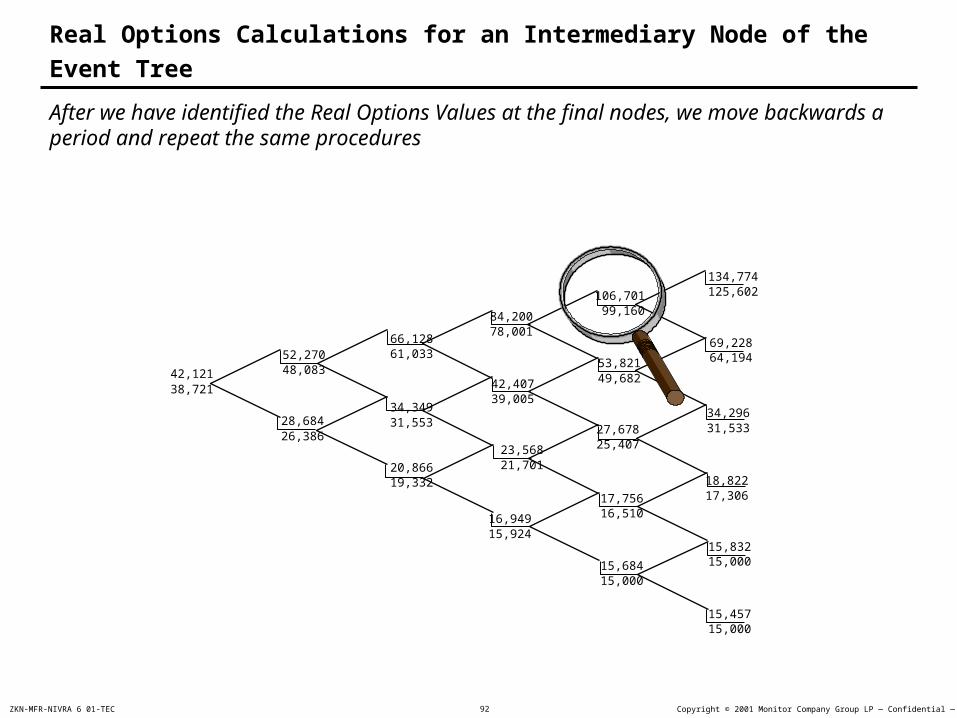
Copyright © 2001 Monitor Company Group LP — Confidential — CAMZKN-MFR-NIVRA 6 01-TEC 92
Real Options Calculations for an Intermediary Node of the Event Tree
134,774
106,701 125,602
84,200 99,160
69,22866,12878,001
53,821 64,19452,270 61,033
42,407 49,682
34,296
42,121 48,083
34,34939,005
27,678 31,533
38,721
28,684 31,553
23,568 25,407
18,822
26,386
20,866 21,701
17,756 17,30619,332
16,949 16,510
15,83215,924
15,684 15,000
15,000
15,45715,000
After we have identified the Real Options Values at the final nodes, we move backwards a period and repeat the same procedures

Copyright © 2001 Monitor Company Group LP — Confidential — CAMZKN-MFR-NIVRA 6 01-TEC 93
First we have to find the replication value for the node
The maximum value of the project after paying out free cash flow is the maximum of its intrinsic value and the values of the expansion or abandonment options
The total PV of a project at this point is the maximum present value plus the free cash flow
Real Options Calculations for An Intermediary Node of the Event Tree
(cont.)
)000,15/160,99/633,97(160,99
000,15/500,10%)301(*354,84/633,97
Max
MaxMaxValue
n=(134,774-69,228)/(113,865-62,491)=1.276
B=(134,774-1.276*113,865)e-.05 =-9,988
ROV = 1.276*84,354-9,988 =97,633
541,7160,99701,106

Copyright © 2001 Monitor Company Group LP — Confidential — CAMZKN-MFR-NIVRA 6 01-TEC 94
Outputs from the Real Options Analysis: Optimal Execution
Expand
OPTIMAL REAL OPTION EXECUTION Expand
Expand Expand
Expand Expand
Go Go Go
Go Go Go
Go Go Go
Go Go
Go Abandon
Abandon
Abandon
Year 1 2 3 4 5 6
Both the option to expand and the option to abandon add to the flexibility of the project as they will be executed in many possible scenarios
As can be expected, the option to expand will be optimally executed if the project does well and the option to abandon if it does badly

Copyright © 2001 Monitor Company Group LP — Confidential — CAMZKN-MFR-NIVRA 6 01-TEC 95
Outputs from the Real Options Analysis: Project’s Value with Flexibility
Because of the project’s high level of uncertainty, the flexibility has added a significant value to its NPV
By enhancing the project’s upside in case of success, and bounding the down side in case of failure, the options have moved its net present value from negative $319,000 to positive $1,986,000
ROA vs. NPV
ROV
No Follow-up
$
$1,986
($319)
($500) $0 $500 $1,000 $1,500 $2,000 $2,500

Copyright © 2001 Monitor Company Group LP — Confidential — CAMZKN-MFR-NIVRA 6 01-TEC 96
Insights
1. NPV requires mutually exclusive alternatives, ROA does not. For example consider a deferral option
NPV Mutually Exclusive AlternativesNPV Mutually Exclusive Alternatives
MAX0 E [NPVt] = NPV < ROA=E [MAXt NPVt]
Defer
Defer
Defer
Defer
Defer
Invest
Invest
Abandon
InvestDefer
The value with flexibility is always greater than the value without. Furthermore, The ROA results yielddecision rules regarding what action to take in each future state of nature
2. Capital spending should be evaluated as a program rather than one project at a time. If we are evaluating a CAPEX program; we should take into account a variety of flexibilities
Excess capacity vs. inventories Economics of scale vs. smaller plants more geographically diverse
ROA Decision TreeROA Decision Tree
NPV0
NPV1
NPV2
NPVN
Start immediately
Defer one year
Defer two years
MAX0
Defer N years
.
.
.
Copyright © 2001 Monitor Company Group LP — Confidential — CAMZKN-MFR-NIVRA 6 01-TEC 97
Issues
Much remains to be done
1. Game theory and real options
2. Path dependent solutions
3. More than two discontinuous sources of uncertainty


![Massachusetts Military Reservation · Otis Air National Guard/Camp Edwards, Falmouth, Massachusetts (Massachusetts Military Reservation [MMR], Cape Cod, Massachusetts)](https://img.pdfslide.us/doc/110x75/5af853a37f8b9a44658c3974/massachusetts-military-reservation-air-national-guardcamp-edwards-falmouth-massachusetts.jpg)