Today in Astronomy 102: relativity and the Universeteacher.pas.rochester.edu/ast102/lecturenotes/lecture22/lecture22.pdfToday in Astronomy 102: relativity and the Universe q General

Lecture 22 Astronomy 102 1

Today in Astronomy 102: relativity and the Universe

q General relativity and the Universe.

q Hubble: the Universe is observed to be homogeneous, isotropic, and expanding

q Redshift and distance: Hubble’s Law Visible-light spectrum of the quasar 3C 273

(Maarten Schmidt, 1963).


General relativity and the Universe

It was recognized soon after Einstein’s invention of the general theory of relativity in 1915 that this theory provides the best framework in which to study the large-scale structure of the Universe: q Gravity is the only force known (then or now) that is long

-ranged enough to influence objects on scales much larger than typical interstellar distances. All the other forces (electricity, magnetism and the nuclear forces) are “shielded” in large accumulations of material or are naturally short ranged.

q And there’s lots of matter around to serve as gravity’s source. Einstein himself worked mostly on this application of GR, rather than on “stellar” applications like black holes. The results wind up having a lot in common with black holes, though.


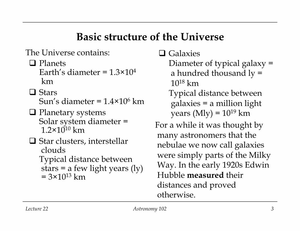
Basic structure of the Universe The Universe contains: q  Planets

Earth’s diameter = 1.3×104

km q  Stars

Sun’s diameter = 1.4×106 km q  Planetary systems

Solar system diameter = 1.2×1010 km

q  Star clusters, interstellar clouds Typical distance between stars = a few light years (ly) = 3×1013 km

q Galaxies Diameter of typical galaxy = a hundred thousand ly = 1018 km Typical distance between galaxies = a million light years (Mly) = 1019 km

For a while it was thought by many astronomers that the nebulae we now call galaxies were simply parts of the Milky Way. In the early 1920s Edwin Hubble measured their distances and proved otherwise.


The Universe is full of galaxies, and to observe them is to probe the structure of

the Universe. This is the HST Ultradeep Field (Beckwith et al., NASA/STScI). Only a few stars are present; virtually every dot is a galaxy. If the whole sky were imaged with the same sensitivity and the galaxies counted, we’d get several hundred billion.


General relativity and the structure of the Universe

The Universe is not an isolated, distinct object like those we’ve dealt with hitherto. In its description we would be interested in the large-scale patterns and trends in gravity (or spacetime curvature). Why? q These trends would tell us how galaxies and groups of

galaxies – the most distant and massive things we can see – would tend to move around in the Universe, and why we see groups of the size we do: this study is called cosmology.

q They might also tell us about the Universe’s origins and fate: this is called cosmogony.

q By large-scale, we mean sizes and distance large compared to the typical distance between galaxies.


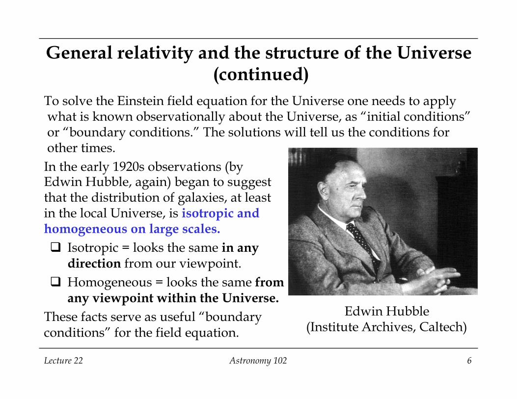
General relativity and the structure of the Universe (continued)

To solve the Einstein field equation for the Universe one needs to apply what is known observationally about the Universe, as “initial conditions” or “boundary conditions.” The solutions will tell us the conditions for other times. In the early 1920s observations (by Edwin Hubble, again) began to suggest that the distribution of galaxies, at least in the local Universe, is isotropic and homogeneous on large scales. q  Isotropic = looks the same in any

direction from our viewpoint. q  Homogeneous = looks the same from

any viewpoint within the Universe. These facts serve as useful “boundary conditions” for the field equation.

Edwin Hubble (Institute Archives, Caltech)


Isotropy of the Universe on large scales: modern measurements

Here positions are marked for galaxies lying within a 6ox6o

patch of the sky: the galaxies are essentially randomly, and uniformly, distributed. (From F. Shu, The Physical Universe.) For scale:

0.5o

(size of the full moon)


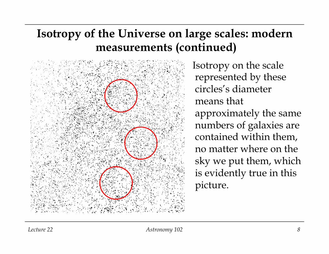
Isotropy of the Universe on large scales: modern measurements (continued)

Isotropy on the scale represented by these circles’s diameter means that approximately the same numbers of galaxies are contained within them, no matter where on the sky we put them, which is evidently true in this picture.


Homogeneity of the Universe on large scales: modern measurements

The Las Campanas Redshift Survey, showing the positions, out to distances of about 3x109

light years along the line of sight, of almost 24,000 galaxies in six different thin stripes on the sky. Data from stripes in the northern and southern sky are overlaid. Again, the galaxies and their larger groupings tend to be randomly distributed through volume on large scales. From Huan Lin, U. Toronto.


Homogeneity of the Universe on large scales: modern measurements (continued)

Homogeneity on the scale of these circles’s diameter means that approximately the same numbers of galaxies are contained within them, no matter where we put them within the Universe’s volume, which is evidently true in this picture. q  Hubble actually demonstrated

this a bit differently: he observed that fainter galaxies (same as brighter ones, but further away) appear in greater numbers than brighter galaxies, by the amount that would be expected if the galaxies are distributed uniformly in space.


Back to general relativity and the structure of the Universe …

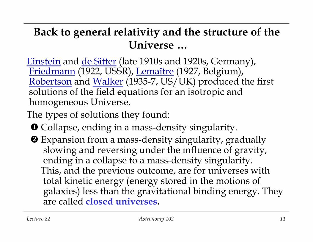
Einstein and de Sitter (late 1910s and 1920s, Germany), Friedmann (1922, USSR), Lemaître (1927, Belgium), Robertson and Walker (1935-7, US/UK) produced the first solutions of the field equations for an isotropic and homogeneous Universe. The types of solutions they found: u Collapse, ending in a mass-density singularity. v Expansion from a mass-density singularity, gradually

slowing and reversing under the influence of gravity, ending in a collapse to a mass-density singularity. This, and the previous outcome, are for universes with total kinetic energy (energy stored in the motions of galaxies) less than the gravitational binding energy. They are called closed universes.


General relativity and the structure of the Universe (continued)

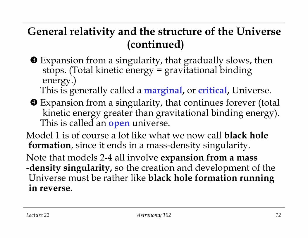
w Expansion from a singularity, that gradually slows, then stops. (Total kinetic energy = gravitational binding energy.) This is generally called a marginal, or critical, Universe.

x Expansion from a singularity, that continues forever (total kinetic energy greater than gravitational binding energy). This is called an open universe.

Model 1 is of course a lot like what we now call black hole formation, since it ends in a mass-density singularity. Note that models 2-4 all involve expansion from a mass-density singularity, so the creation and development of the Universe must be rather like black hole formation running in reverse.


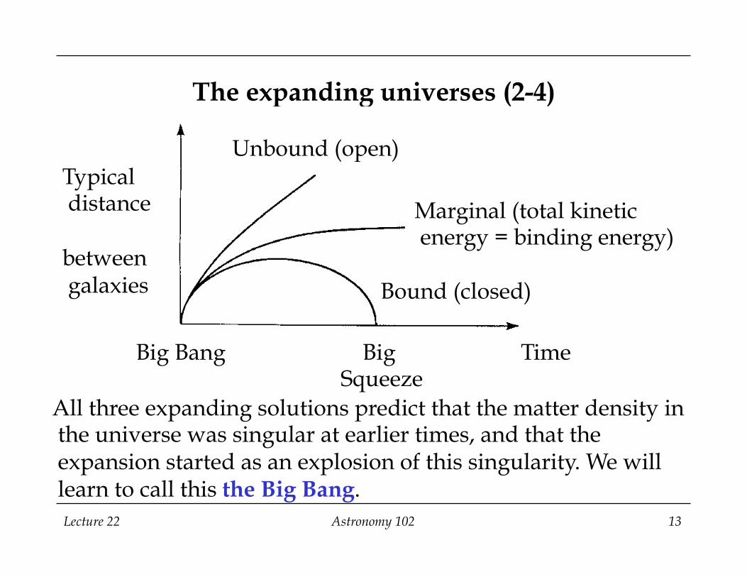
The expanding universes (2-4)

All three expanding solutions predict that the matter density in the universe was singular at earlier times, and that the expansion started as an explosion of this singularity. We will learn to call this the Big Bang.

Typical distance between galaxies

Time

Unbound (open)

Bound (closed)

Marginal (total kinetic energy = binding energy)

Big Bang Big Squeeze


Einstein doesn’t like it.

Big surprise. All the solutions have these features in common: q mass-density singularities, and q  dynamic behavior: the structure given by the solutions is

different at different times between singularities (at which time doesn’t exist, of course).

Einstein thought that singularities such as these indicated that there were important physical effects not accounted for in the field equation. He had a hunch that the right answer would involve static behavior: large-scale structure should not change with time. q He also saw how he could “fix” the field equation to eliminate

singular and dynamic solutions: introduce an additional constant term, which became known as the cosmological constant, to represent the missing, unknown, physical effects.


The field equation and the cosmological constant: hieroglyphics (i.e. not on the exam or homework) The field equation under a particularly simple set of assumptions and conditions for a homogeneous and isotropic Universe: The same equation modified by Einstein (1917):

22

21 8

3dR G k

cR dt R

π ρ⎛ ⎞ − = −⎜ ⎟⎝ ⎠

Typical distance between galaxies

Mass density (mass per unit volume)

Space (3-D) curvature

1R

dRdt

⎛⎝⎜

⎞⎠⎟

2

− 8πG3

ρ − c2

3Λ = −c2 k

R2

Cosmological constant A certain positive value of Λ leads a static solution.


Mid-lecture Break (4 min. 4 sec.)

This is Edwin Hubble, pretending he’s observing at the Newtonian focus of the Mt. Wilson 100-inch Telescope. It would be dark if he were really observing, of course. (Institute Archives, Caltech)

Homework Set #5 is due on Saturday 4/16 at 8.30 am. Homework Set # 6 is due on Saturday 4/23 at 8.30 am.


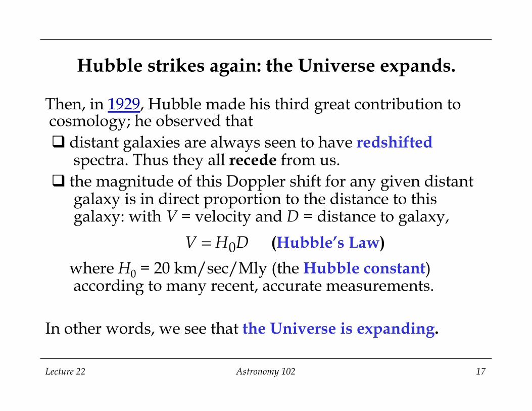
Hubble strikes again: the Universe expands.

Then, in 1929, Hubble made his third great contribution to cosmology; he observed that q distant galaxies are always seen to have redshifted

spectra. Thus they all recede from us. q the magnitude of this Doppler shift for any given distant

galaxy is in direct proportion to the distance to this galaxy: with V = velocity and D = distance to galaxy, where H0 = 20 km/sec/Mly (the Hubble constant) according to many recent, accurate measurements.

In other words, we see that the Universe is expanding.

V H D= 0 (Hubble’s Law)


Why galaxies recede from an observer in the expanding Universe, no matter where she stands.

Universal expansion

A

B

A’

B’

All intergalaxy distances increase: A’ > A, B’ > B. (The galaxies themselves do not expand, though.)


Why galaxies recede from an observer in the expanding Universe, no matter where she stands.

A

B

A’

B’

Galaxies recede from one another, and recede faster the further apart they are: B’-B > A’-A. Because the galaxies recede, the Doppler shifts are all redshifts.

Universal expansion


Hubble’s Law

0 ,V H D=

Here are Hubble’s and Humason’s original (1929) data and result. Clearly the straight line is a good fit, so though the slope (the Hubble constant) came out a lot larger than in recent measurements, due to then-unforseen systematic distance errors.

Graph from Ned Wright’s Cosmology Tutorial.

(1Mpc = 3.26 Mly)


Hubble-constant determination, using Type Ia supernovae in galaxies to measure distance

0-1 -1

19.6 0.9

km sec Mly

H = ±

In AST 102, we will use a round number:

-1 -10 20 km sec MlyH =

Nowadays, better distance measurements and a better fit:

Riess, Press and Kirschner 1996 Graph from Ned Wright’s Cosmology Tutorial.

(1Mpc = 3.26 Mly)


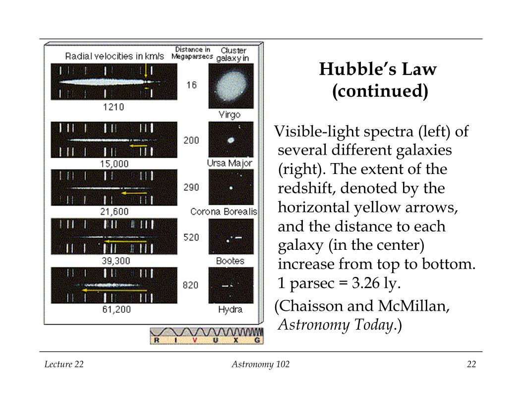
Hubble’s Law (continued)

Visible-light spectra (left) of several different galaxies (right). The extent of the redshift, denoted by the horizontal yellow arrows, and the distance to each galaxy (in the center) increase from top to bottom. 1 parsec = 3.26 ly. (Chaisson and McMillan, Astronomy Today.)


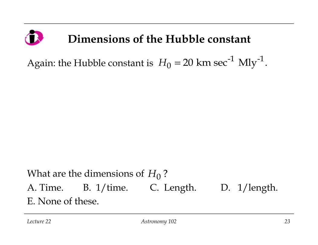
Dimensions of the Hubble constant

Again: the Hubble constant is What are the dimensions of A. Time. B. 1/time. C. Length. D. 1/length. E. None of these.

-1 -10 20 km sec Mly .H =

0 ?H


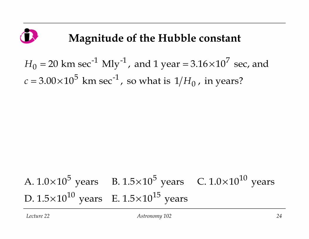
Magnitude of the Hubble constant

-1 -1 70

5 -10

20 km sec Mly , and 1 year 3.16 10 sec, and

3.00 10 km sec , so what is 1 , in years?

H

c H

= = ×

= ×

5 5 10

10 15

A. 1.0 10 years B. 1.5 10 years C. 1.0 10 years

D. 1.5 10 years E. 1.5 10 years

× × ×

× ×

( )0

6 5 -1

10

sec Mly1

20 km

sec 10 3 10 km sec year

20 km1.5 10 year.

H =

× × × ×=

= ×


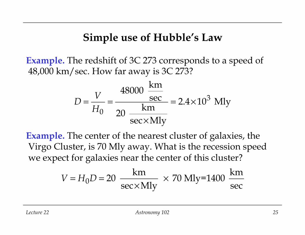
Example. The redshift of 3C 273 corresponds to a speed of 48,000 km/sec. How far away is 3C 273? Example. The center of the nearest cluster of galaxies, the Virgo Cluster, is 70 Mly away. What is the recession speed we expect for galaxies near the center of this cluster?

Simple use of Hubble’s Law

3

0

km48000 sec 2.4 10 Mly

km20 sec Mly

VD

H= = = ×

×

0km km

20 70 Mly=1400 sec Mly sec

V H D= = ××


Distances from redshifts

The velocities of galaxies in a certain galaxy cluster average to 30,000 km/sec. How far away is the cluster? A. 1100 Mly B. 1200 Mly C. 1300 Mly D. 1400 Mly E. 1500 Mly


Einstein gives up.

The Universe is observed to be expanding; it is not static. q  Thus the real Universe may be described by one

of the dynamic solutions to the original Einstein field equation. Of the four types we discussed above, the last three spend at least part of their time, if not all, expanding.

q  And thus there appeared to be no point in Einstein’s cosmological constant, so he let it drop, calling it “my greatest blunder” in an oft-quoted elevator conversation.

q  Thereafter he began trying to show that the singularities in the dynamic solutions simply wouldn’t be realized. His effort resulted in the steady-state model of the Universe, which we’ll describe later.

This isn’t the last we’ll see of the cosmological constant, though.


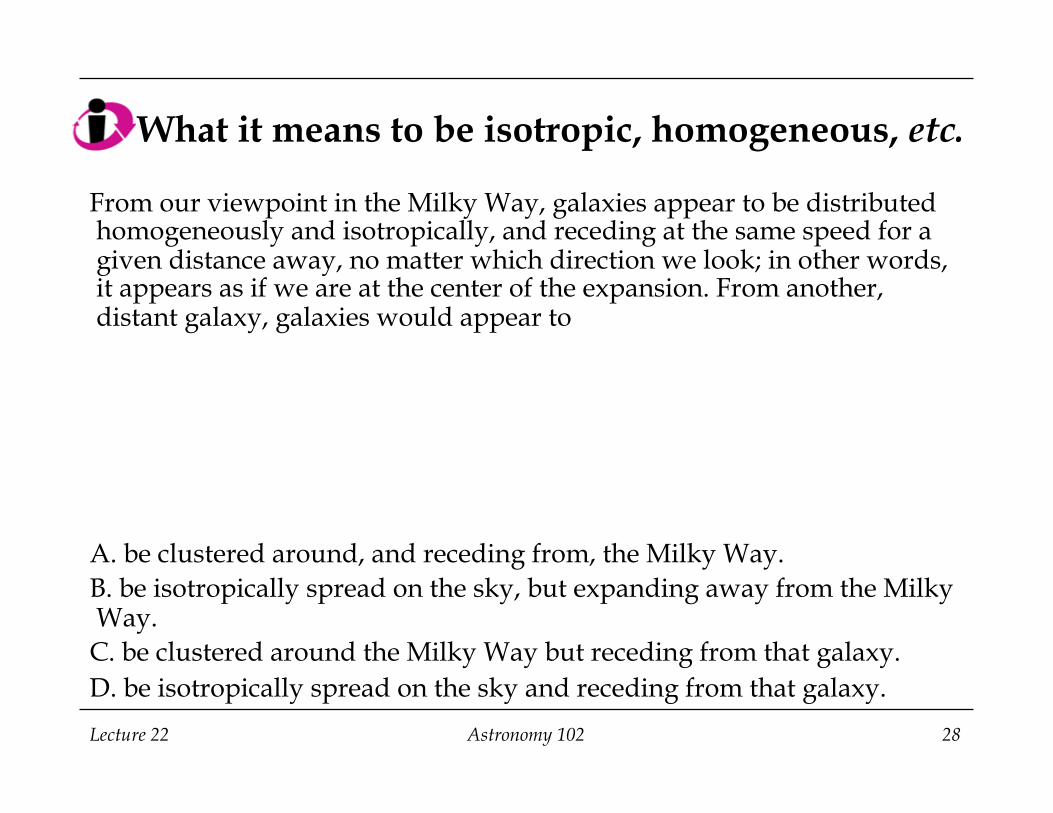
What it means to be isotropic, homogeneous, etc.

From our viewpoint in the Milky Way, galaxies appear to be distributed homogeneously and isotropically, and receding at the same speed for a given distance away, no matter which direction we look; in other words, it appears as if we are at the center of the expansion. From another, distant galaxy, galaxies would appear to A. be clustered around, and receding from, the Milky Way. B. be isotropically spread on the sky, but expanding away from the Milky Way. C. be clustered around the Milky Way but receding from that galaxy. D. be isotropically spread on the sky and receding from that galaxy.


Summary of Hubble’s findings

q The Universe is isotropic: on large scales it looks the same in all directions, from our viewpoint.

q The Universe is homogeneous: it is uniform on large scales. In other words, the Universe looks the same from any viewpoint.

q The Universe is expanding: •  The galaxies recede from us, faster the further away

they are. •  And since the Universe is homogeneous, we would see

the same recession no matter where we stood. That is, there is no unique center in space, of the expansion, as in an ordinary explosion and blast wave.

Done! Comet Hale-Bopp Over Indian Cove


Image Credit & Copyright: Wally Pacholka (Astropics, TWAN)

Documents

Today in Astronomy 102: relativity and the Universeteacher.pas.rochester.edu/ast102/lecturenotes/lecture22/lecture22.pdfToday in Astronomy 102: relativity and the Universe q General