Embed Size (px)
Citation preview
P10, Fall 2016 – Spring 2017
ToA Path Estimation for IndoorPositioning
Using MUSIC algorithm for Time Resolution Enhancement
WCS10 - Group 1051
8th June 2017

Antennas, Propagation and RadioNetworking (APNet) Department of
Electronic SystemsFredrik Bajers Vej 7DK-9220 Aalborg Ø
http://es.aau.dk
Title:ToA Path Estimation for Indoor Position-ingUsing MUSIC algorithm for Time Resolu-tion Enhancment
Theme:Wireless Communication Systems
Project Period:P10, Fall 2016 - spring 2017
Project Group:1051
Author:Mathias Hjorth Laursen
Supervisor:Troels Bundgaard Sørensen
Pages: 71
Date of Completion:8th June 2017
Abstract:
Due to the increasing demand for indoorpositioning or navigation systems this the-sis investigates the possibilities of creatingan indoor positioning system using a com-bination of ToA and the MUSIC algorithmfor increased time resolution. The charac-teristics of the wireless transmission chan-nel are investigated as these can be usedfor creating end evaluating an indoor po-sitioning system.A model describing a ToA system is devel-oped. Simulations of this model was madein order to evaluate the impact of dif-ferent wireless characteristics, especiallythe ToA between different reflected signalpaths and the improvements made by theMUSIC algorithm. Measurements weremade to evaluate the performance of theMUSIC algorithm on a wireless channelin LOS and NLOS scenarios. Test resultsshows a significant improvement by usinga combination of ToA and the MUSIC al-gorithm compared with a traditional ToApositioning system.
The content of this report is freely available, but publication (with reference) may only be pursued due to
agreement with the author.

Preface
The following master thesis covers the project made by Mathias Laursen to complete hisWireless Communication Systems Master’s program at Aalborg university. The topic ofthe thesis is indoor localisation based on wireless channel characteristics and complexcomputation algorithm to enhance accuracy.
The author would like to thank Thomas Lundgaard Hansen for his help within the fieldof signal processing.
The report is divided into 2 overall parts, first chapter 1-3 introduces the concept of indoorlocalisation together with a basic evaluation of different wireless channel characteristicsto use for position estimation. Following chapter 4-5 describes a system model for sim-ulating Time of Arrival as a wireless channel characteristic to improve the accuracy ofindoor location system by using the MUSIC algorithm to enhance the time resolution ofa measured wireless channel. Part to results in an evaluation of empirical and simulatedwireless channels and the ability to make precise positioning using time of arrival.
Citations are made by the use of American Institute of Physics (AIP) style. This stylerepresents a citation by the use of only a number e.g. [13] which refers to the 13.th entryin the bibliography found in the end of the thesis. Adding the number before a full stope.g. a dot as ”[ ].” the citation refers only to that sentence and adding it after full stopthe citation is referring for the full paragraph.
For table, figure and equation references the following approach is used e.g. figure x,yrefers to the y’th figure in chapter x. Similar for the table and equations.
Aalborg University, Denmark, June 8th 2017.
v

Contents
1 Introduction 11.1 Background . . . . . . . . . . . . . . . . . . . . . . . . . . . . . . . . . . . 11.2 Thesis Contribution . . . . . . . . . . . . . . . . . . . . . . . . . . . . . . . 41.3 Thesis Overview . . . . . . . . . . . . . . . . . . . . . . . . . . . . . . . . . 4
2 Indoor Localisation 52.1 Definition Overview . . . . . . . . . . . . . . . . . . . . . . . . . . . . . . . 52.2 Description of Localisation Methods . . . . . . . . . . . . . . . . . . . . . . 7
2.2.1 Proximity Detection . . . . . . . . . . . . . . . . . . . . . . . . . . 72.2.2 Lateration . . . . . . . . . . . . . . . . . . . . . . . . . . . . . . . . 82.2.3 Scene analysis . . . . . . . . . . . . . . . . . . . . . . . . . . . . . . 92.2.4 Summary of Localisation Methods . . . . . . . . . . . . . . . . . . . 11
2.3 Obtaining Input Data . . . . . . . . . . . . . . . . . . . . . . . . . . . . . 122.3.1 ToA . . . . . . . . . . . . . . . . . . . . . . . . . . . . . . . . . . . 122.3.2 AoA . . . . . . . . . . . . . . . . . . . . . . . . . . . . . . . . . . . 142.3.3 RSSI . . . . . . . . . . . . . . . . . . . . . . . . . . . . . . . . . . . 14
2.4 Performance Measure . . . . . . . . . . . . . . . . . . . . . . . . . . . . . . 15
3 Simulations of Basic Localisation Methods 173.1 AoA . . . . . . . . . . . . . . . . . . . . . . . . . . . . . . . . . . . . . . . 17
3.1.1 Conclusion of AoA . . . . . . . . . . . . . . . . . . . . . . . . . . . 213.2 RSSI . . . . . . . . . . . . . . . . . . . . . . . . . . . . . . . . . . . . . . . 21
3.2.1 Fingerprinting . . . . . . . . . . . . . . . . . . . . . . . . . . . . . . 223.2.2 Distance Propagation Method . . . . . . . . . . . . . . . . . . . . . 233.2.3 Conclusion of RSSI . . . . . . . . . . . . . . . . . . . . . . . . . . . 25
3.3 ToA . . . . . . . . . . . . . . . . . . . . . . . . . . . . . . . . . . . . . . . 253.4 Conclusion of Basic Localisation methods . . . . . . . . . . . . . . . . . . . 27
4 ToA Positioning with Time Resolution Enhancement 294.1 I/Q baseband description . . . . . . . . . . . . . . . . . . . . . . . . . . . . 294.2 System Model . . . . . . . . . . . . . . . . . . . . . . . . . . . . . . . . . . 304.3 Identification data . . . . . . . . . . . . . . . . . . . . . . . . . . . . . . . 314.4 Gold Code PRN Sequence . . . . . . . . . . . . . . . . . . . . . . . . . . . 324.5 Channel . . . . . . . . . . . . . . . . . . . . . . . . . . . . . . . . . . . . . 364.6 Correlator/despreading . . . . . . . . . . . . . . . . . . . . . . . . . . . . . 374.7 MUSIC Algorithm . . . . . . . . . . . . . . . . . . . . . . . . . . . . . . . 39
4.7.1 Decorrelating the Covariance Matrix . . . . . . . . . . . . . . . . . 42
vii
CONTENTS
5 MUSIC Algorithm Performance Analysis 435.1 Analytical 2-path tests . . . . . . . . . . . . . . . . . . . . . . . . . . . . . 445.2 Experimental evaluation of MUSIC algorithm . . . . . . . . . . . . . . . . 475.3 Correlation impact . . . . . . . . . . . . . . . . . . . . . . . . . . . . . . . 505.4 Measurement precision and accuracy . . . . . . . . . . . . . . . . . . . . . 515.5 Signal Space Evaluation . . . . . . . . . . . . . . . . . . . . . . . . . . . . 52
6 Conclusion 556.1 Future Work . . . . . . . . . . . . . . . . . . . . . . . . . . . . . . . . . . . 56
A Channel Measurement Description 61A.1 Purpose of Measurements . . . . . . . . . . . . . . . . . . . . . . . . . . . 61A.2 Setup . . . . . . . . . . . . . . . . . . . . . . . . . . . . . . . . . . . . . . . 61A.3 Data processing . . . . . . . . . . . . . . . . . . . . . . . . . . . . . . . . . 63A.4 Channel Impulse Responses and Frequency Sweeps . . . . . . . . . . . . . 64A.5 Coherence Bandwidth . . . . . . . . . . . . . . . . . . . . . . . . . . . . . 66
B Impact of Indoor Environment 69
viii
CONTENTS
Abbreviations
AoA angle of arrival
AWGN additive white gaussion noise
CDF cumulative distribution function
DDE distance determination error
DDP dominant direct path
EVD eigenvalue decomposition
FCF frequency correlation function
GPS global positioning system
IPS indoor positioning system
kNN k-Nearest Neighbour
LOS line of sight
MT mobile terminal
MUSIC MUltiple SIgnal Classification
NDDP non dominant direct path
NLOS no line of sight
PDE Position determination error
PRN pseudo random noise
RSSI received signal strength indicator
RTT round trip time
TDoA time difference of arrival
ToA time of arrival
ToF time of flight
UDP undetected direct path
UWB Ultra Wideband
WSSUS wide sense stationary uncorrelated scattering
ix

CONTENTS
List of Symbols
A amplitude
α attenuation
B bandwidth
c speed of light
h channel impulse response
d true distance
∆t time difference
derr synchronization error
d distance estimate
δ dirac pulse
µθ mean angular distribution
p position estimate
p true position
σθ angular standard deviation
τ propagation delay
θ angle
ttravel time traveled
x
Chapter 1
Introduction
1.1 Background
In recent years the usage of positioning data has increased in a variety of applications.Often outdoor applications perform well by utilising global positioning system (GPS) orsimilar outdoor positioning systems. However for the application of indoor localisation ornavigation the GPS system does not provide satisfying accuracy. To achieve high accuracyin an indoor environment a dedicated system has to be created which takes into accountthe complexity of an indoor environment.
The need for indoor positioning systems is a increasingly growing market [1].
Indoor positioning system (IPS) has a wide range of applications and application areas.Below are listed some different scenarios where localisation could provide increased cus-tomer experience, ease of work, or new application could be designed based on positionknowledge. Such systems could be tracking positions or navigation:
• In the healthcare industry an accurate localisation system could provide easier pa-tients tracking for hospitals, or for tracking demented people. Similar the systemcould be used for localising staff or equipment, or help patients and relatives navi-gate the area.• For places like airports, museums or subways a localisation system can also help
provide guidance. This could be for guiding people to their gates in the airports,the correct train in the subway or grant a guided tour through museums and similar.• In warehouses the system could be used for tracking incoming and outgoing pack-
ets/orders/etc. And to keep the location of different wares known, so that packingof orders eases. In larger warehouses or factories, localisations of tools or differentmachines would also possible.• At shopping malls or grocery stores a tracking system could also help people find
the different wares they are searching, or the system could in cooperation with ashopping list, create the fastest way through the stores to get all wares listed.• Lastly an IPS can be used for gathering positioning data for all kind of different
1
1.1. BACKGROUND
locations. This could help provide a lot of statistical usage and applications. e.g.knowing the positions of customers in a shopping mall, grants the possibility forplacing different wares strategically to sell more.
The need for more advanced and accurate positioning systems than those already designedis needed. The systems already designed are based on a set of different technologies thatcan be used to create an IPS. A list of technologies is found below [2].
• Satellite based navigation• Inertial navigation system• Sound based navigation• Optical based navigation• Electromagnetic wave based navigation• Magnetic based navigation• Infrastructure system based navigation
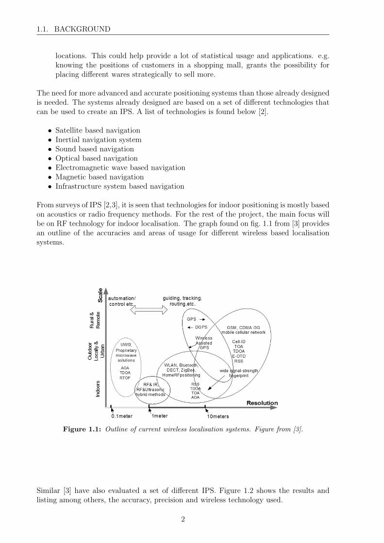
From surveys of IPS [2,3], it is seen that technologies for indoor positioning is mostly basedon acoustics or radio frequency methods. For the rest of the project, the main focus willbe on RF technology for indoor localisation. The graph found on fig. 1.1 from [3] providesan outline of the accuracies and areas of usage for different wireless based localisationsystems.
Figure 1.1: Outline of current wireless localisation systems. Figure from [3].
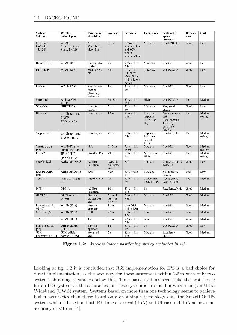
Similar [3] have also evaluated a set of different IPS. Figure 1.2 shows the results andlisting among others, the accuracy, precision and wireless technology used.
2
1.1. BACKGROUND
Figure 1.2: Wireless indoor positioning survey evaluated in [3].
Looking at fig. 1.2 it is concluded that RSS implementation for IPS is a bad choice fordirect implementation, as the accuracy for these systems is within 2-5 m with only twosystems obtaining accuracies below this. Time based systems seems like the best choicefor an IPS system, as the accuracies for these system is around 1 m when using an UltraWideband (UWB) system. Systems based on more than one technology seems to achievehigher accuracies than those based only on a single technology e.g. the SmartLOCUSsystem which is based on both RF time of arrival (ToA) and Ultrasound ToA achieves anaccuracy of <15 cm [4].
3
1.2. THESIS CONTRIBUTION
1.2 Thesis Contribution
The contribution of the thesis is an evaluation of a method to obtain accurate positionestimates by exploiting the signal properties for the ToA of wireless channels. First anevaluation is performed to isolate what initially seems to be the best wireless character-istic for creating an IPS. Afterwards this characteristic is further analysed and the highresolution MUSIC algorithm is used to further improve the position detection ability.Measurement and evaluations of the wireless channel in different LOS and NLOS areevaluated w.r.t. the MUSIC signal processing algorithm. Different input parameters forthe complex algorithm are evaluated to measure the performance in the different LOS andNLOS scenarios. Paremeters tested are SNR, samples, bandwidth and specific parameterestimation for the MUSIC algorithm.
1.3 Thesis Overview
The remaining chapters for the thesis will be as follows; Chapter 2 describes the basicterms used in localisation, afterwards is a description of the different localisation methodswhich can be utilised for calculating a position and the chapter ends with a description ofthe different wireless channel characteristics that can be utilised to obtain input data forthe localisation methods. Chapter 3 evaluates the input data and the errors introduced bythese due to changes in the wireless channel. From the conclusion that the ToA systemseems to achieve best performance, chapter 4 describes a ToA system model and howto measure this. After the high resolution algorithm is described. Section 5.1 describesthe evaluation of the MUSIC algorithm w.r.t. the different parameters that changes theperformance of this. Both simulated and empirical data is evaluated. Chapter 6 concludesthe project and describes future work which could be made.
4
Chapter 2
Indoor Localisation
The following chapter is structured as follows. Section 2.1 will provide an overview ofthe different terms used in the project. Section 2.2 provides an overview of the differentpositioning methods used e.g. lateration and fingerprinting. Section 2.3 explains thedifferent wireless characteristics which can be used to obtain data for the positioningmethods. Section 2.4 describes the performance measure for the different IPS examined.
2.1 Definition Overview
To better understand what an indoor positioning system(IPS) is, it is important to knowthe most commonly used expressions and definitions.
Tag is used to describe the transmitting/receiving devices mounted on people or equip-ment to track locations. The tag is both used for description of a dummy-transmittingdevice and a smart device, which could include both transmitting, receiving and cal-culating capabilities. It is also known as a mobile terminal (MT) or a transceiver.
Nodes are the devices, which receives the transmitted signal from the tag, or in somesituations transmits a signal to the tag. The nodes also in most cases calculatesthe position of the tag or forwards the data to a server, depending on the systemarchitecture. Nodes are placed in known positions for the system to have referencepoints when calculating the tag position. In other context the nodes are denotedbase stations, reference points or gateways.
IPS can be created in different fashions, most commonly it consists of a set of tags (thedevices which location /position are wanted) and a set of nodes which are referencepoints and the sampling system used to estimate the position of the tags. IPS isused to denote a system which is capable of locating people or objects in an indoorenvironment mounted with tags. The positioning capability is measured both byaccuracy and precision of the system.
Accuracy is the mean distance error between estimated locations and the true locations.Accuracy describes how far off the mean from a set of measurements is from the
5
2.1. DEFINITION OVERVIEW
true location, thereby it can be seen as a offset error in the IPS. The accuracy of asystem is closely related to, but it not equal to the precision.
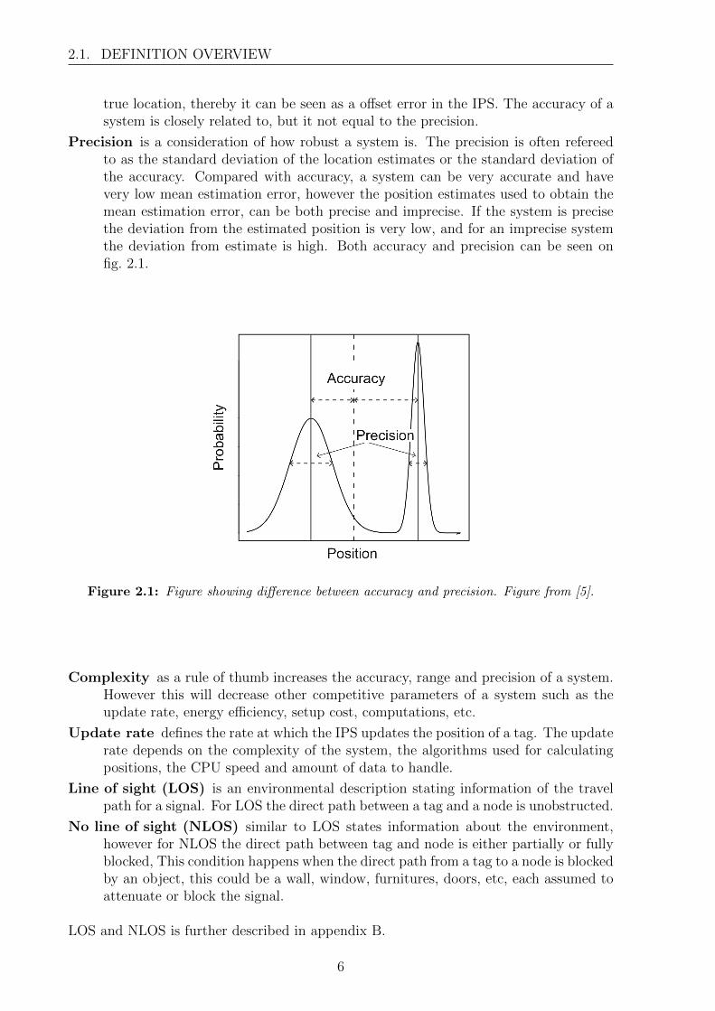
Precision is a consideration of how robust a system is. The precision is often refereedto as the standard deviation of the location estimates or the standard deviation ofthe accuracy. Compared with accuracy, a system can be very accurate and havevery low mean estimation error, however the position estimates used to obtain themean estimation error, can be both precise and imprecise. If the system is precisethe deviation from the estimated position is very low, and for an imprecise systemthe deviation from estimate is high. Both accuracy and precision can be seen onfig. 2.1.
Figure 2.1: Figure showing difference between accuracy and precision. Figure from [5].
Complexity as a rule of thumb increases the accuracy, range and precision of a system.However this will decrease other competitive parameters of a system such as theupdate rate, energy efficiency, setup cost, computations, etc.
Update rate defines the rate at which the IPS updates the position of a tag. The updaterate depends on the complexity of the system, the algorithms used for calculatingpositions, the CPU speed and amount of data to handle.
Line of sight (LOS) is an environmental description stating information of the travelpath for a signal. For LOS the direct path between a tag and a node is unobstructed.
No line of sight (NLOS) similar to LOS states information about the environment,however for NLOS the direct path between tag and node is either partially or fullyblocked, This condition happens when the direct path from a tag to a node is blockedby an object, this could be a wall, window, furnitures, doors, etc, each assumed toattenuate or block the signal.
LOS and NLOS is further described in appendix B.
6
2.2. DESCRIPTION OF LOCALISATION METHODS
2.2 Description of Localisation Methods
The following section will describe the algorithms used for estimating the position of atag.
Generally in an IPS, the position of a device is calculated in nodes or in a central server,this is to minimize power consumption of the tag. The reason to use a centralised server isoften a result of dummy-tags and dummy-nodes which are only used for transmitting andreceiving signals, while further handing the received signal to a stronger computationalbackbone for position calculations.
To calculate the a position estimate, different algorithms can be used. Even though thereare a lot of different positioning techniques and systems, they are generally based on thesame limited number of algorithms or variations of these [5].
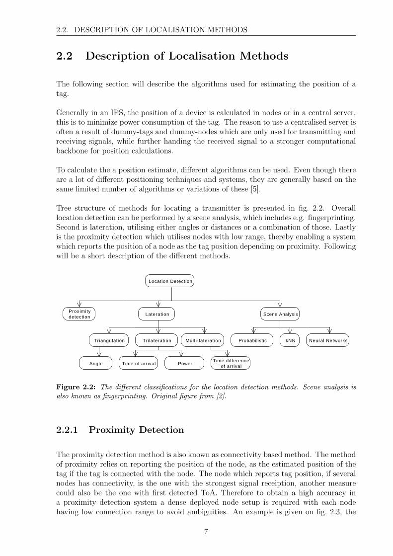
Tree structure of methods for locating a transmitter is presented in fig. 2.2. Overalllocation detection can be performed by a scene analysis, which includes e.g. fingerprinting.Second is lateration, utilising either angles or distances or a combination of those. Lastlyis the proximity detection which utilises nodes with low range, thereby enabling a systemwhich reports the position of a node as the tag position depending on proximity. Followingwill be a short description of the different methods.
Location Detection
Proximitydetection Lateration Scene Analysis
Triangulation Trilateration
Angle Time of arrival Power
Probabilistic kNN Neural NetworksMulti-lateration
Time difference of arrival
Figure 2.2: The different classifications for the location detection methods. Scene analysis isalso known as fingerprinting. Original figure from [2].
2.2.1 Proximity Detection
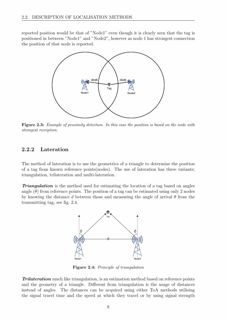
The proximity detection method is also known as connectivity based method. The methodof proximity relies on reporting the position of the node, as the estimated position of thetag if the tag is connected with the node. The node which reports tag position, if severalnodes has connectivity, is the one with the strongest signal receiption, another measurecould also be the one with first detected ToA. Therefore to obtain a high accuracy ina proximity detection system a dense deployed node setup is required with each nodehaving low connection range to avoid ambiguities. An example is given on fig. 2.3, the
7
2.2. DESCRIPTION OF LOCALISATION METHODS
reported position would be that of ”Node1” even though it is clearly seen that the tag ispositioned in between ”Node1” and ”Node2”, however as node 1 has strongest connectionthe position of that node is reported.
Figure 2.3: Example of proximity detection. In this case the position is based on the node withstrongest receiption.
2.2.2 Lateration
The method of lateration is to use the geometrics of a triangle to determine the positionof a tag from known reference points(nodes). The use of lateration has three variants;triangulation, trilateration and multi-lateration.
Triangulation is the method used for estimating the location of a tag based on anglesangle (θ) from reference points. The position of a tag can be estimated using only 2 nodesby knowing the distance d between those and measuring the angle of arrival θ from thetransmitting tag, see fig. 2.4.
Figure 2.4: Principle of triangulation
Trilateration much like triangulation, is an estimation method based on reference pointsand the geometry of a triangle. Different from triangulation is the usage of distancesinstead of angles. The distances can be acquired using either ToA methods utilisingthe signal travel time and the speed at which they travel or by using signal strength
8
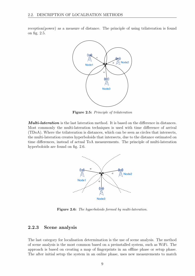
2.2. DESCRIPTION OF LOCALISATION METHODS
reception(power) as a measure of distance. The principle of using trilateration is foundon fig. 2.5.
Figure 2.5: Principle of trilateration
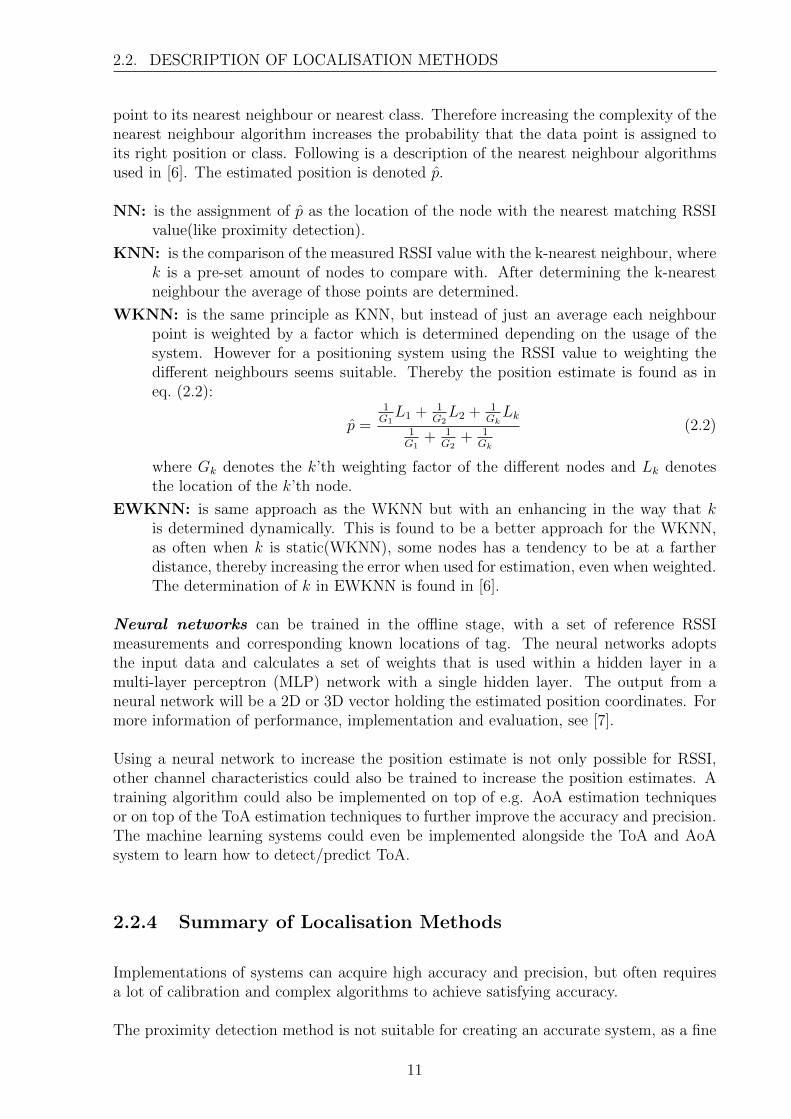
Multi-lateration is the last lateration method. It is based on the difference in distances.Most commonly the multi-lateration techniques is used with time difference of arrival(TDoA). Where the trilateration is distances, which can be seen as circles that intersects,the multi-lateration creates hyperboloids that intersects, due to the distance estimated ontime differences, instead of actual ToA measurements. The principle of multi-laterationhyperboloids are found on fig. 2.6.
Figure 2.6: The hyperboloids formed by multi-lateration.
2.2.3 Scene analysis
The last category for localisation determination is the use of scene analysis. The methodof scene analysis is the most common based on a preinstalled system, such as WiFi. Theapproach is based on creating a map of fingerprints in an offline phase or setup phase.The after initial setup the system in an online phase, uses new measurements to match
9

2.2. DESCRIPTION OF LOCALISATION METHODS
with the fingerprints made in the offline phase. The fingerprints with the best match forthe new measurement is reported as the tag position.
Depending on the accuracy wanted, the fingerprints has to be measured in a equal or finergrid, than the accuracy wanted. This could also be achieved by interpolation the mea-surements between grid points. The fingerprints measured can be different characteristicsof a signal [3], however mostly received signal strength indicator (RSSI) is used. Thefingerprints are stored on a server ready for use with different scene analysis algorithms.A downside on the usage of scene analysis is that the offline phase can be time consumingdepending on the installation area. Also the scene analysis, depending on algorithm, canalso be vulnerable to changes in environment, such as rebuilding a wall or relocating offurnitures/offices or generally movement and changes in environment. Figure 2.7 showsa grid which indicates reference points measured, the grid size can be changed dependingon the accuracy. Large grid size(left) gives less accuracy, small grid size (bottom-middle)grants possibility for higher accuracy.
Figure 2.7: Grid for offline phase of scene analysis, each cross is a measurement point.
The scene analysis method have the offline approach of measuring reference points, how-ever different methods can be utilised for the online phase to make the fingerprint match-ing. The online phase is when system has been calibrated and is ready to position devices.From [3] the following algorithms are examined: probabilistic method, k-Nearest Neigh-bour (kNN) and Machine learning/neural networks.
Probabilistic method considers the probability that given an observed signal strength,s, the position of the tag is located in location Li. A decision rule is made in the offlinephase for creating the fingerprinting map, stating that location, Li is chosen if:
P (Li|s) > P (Lj|s), where j, i = 1, 2, 3.....n (2.1)
where n is the amount of locations. Therefore measuring s, the tag position is reportedas the position L which obtains highest probability.
Nearest neighbour algorithms is a method used for classification, which assigns a data
10
2.2. DESCRIPTION OF LOCALISATION METHODS
point to its nearest neighbour or nearest class. Therefore increasing the complexity of thenearest neighbour algorithm increases the probability that the data point is assigned toits right position or class. Following is a description of the nearest neighbour algorithmsused in [6]. The estimated position is denoted p.
NN: is the assignment of p as the location of the node with the nearest matching RSSIvalue(like proximity detection).
KNN: is the comparison of the measured RSSI value with the k-nearest neighbour, wherek is a pre-set amount of nodes to compare with. After determining the k-nearestneighbour the average of those points are determined.
WKNN: is the same principle as KNN, but instead of just an average each neighbourpoint is weighted by a factor which is determined depending on the usage of thesystem. However for a positioning system using the RSSI value to weighting thedifferent neighbours seems suitable. Thereby the position estimate is found as ineq. (2.2):
p =1G1L1 + 1
G2L2 + 1
GkLk
1G1
+ 1G2
+ 1Gk
(2.2)
where Gk denotes the k’th weighting factor of the different nodes and Lk denotesthe location of the k’th node.
EWKNN: is same approach as the WKNN but with an enhancing in the way that kis determined dynamically. This is found to be a better approach for the WKNN,as often when k is static(WKNN), some nodes has a tendency to be at a fartherdistance, thereby increasing the error when used for estimation, even when weighted.The determination of k in EWKNN is found in [6].
Neural networks can be trained in the offline stage, with a set of reference RSSImeasurements and corresponding known locations of tag. The neural networks adoptsthe input data and calculates a set of weights that is used within a hidden layer in amulti-layer perceptron (MLP) network with a single hidden layer. The output from aneural network will be a 2D or 3D vector holding the estimated position coordinates. Formore information of performance, implementation and evaluation, see [7].
Using a neural network to increase the position estimate is not only possible for RSSI,other channel characteristics could also be trained to increase the position estimates. Atraining algorithm could also be implemented on top of e.g. AoA estimation techniquesor on top of the ToA estimation techniques to further improve the accuracy and precision.The machine learning systems could even be implemented alongside the ToA and AoAsystem to learn how to detect/predict ToA.
2.2.4 Summary of Localisation Methods
Implementations of systems can acquire high accuracy and precision, but often requiresa lot of calibration and complex algorithms to achieve satisfying accuracy.
The proximity detection method is not suitable for creating an accurate system, as a fine
11
2.3. OBTAINING INPUT DATA
grid of reference nodes are required.
Lateration techniques is simple to implement, as the only needed knowledge is the instal-lation locations of nodes and from these a tag position can be estimated.
The neural networks to create an IPS, from [7], seems to acquire high accuracy andprecision at a wide range from 0 m - 100 m. However the offline and training stage istime consuming especially for larger areas. Also the scene analysis techniques are verysensitive to changes in the environment if based on signal strength.
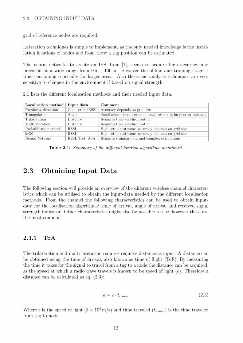
2.1 lists the different localisation methods and their needed input data.
Localisation method Input data CommentProximity detection Connection/RSSI Accuracy depends on grid sizeTriangulation Angle Small measurement error in angle results in large error estimateTrilateration Distance Requires time synchronizationMultilateration Distance Requires time synchronizationProbabilistic method RSSI High setup cost/time, accuracy depends on grid sizekNN RSSI High setup cost/time, accuracy depends on grid sizeNeural Network RSSI, ToA, AoA Requires training data and complex calculations
Table 2.1: Summary of the different location algorithms mentioned.
2.3 Obtaining Input Data
The following section will provide an overview of the different wireless channel character-istics which can be utilised to obtain the input-data needed by the different localisationmethods. From the channel the following characteristics can be used to obtain input-data for the localisation algorithms: time of arrival, angle of arrival and received signalstrength indicator. Other characteristics might also be possible to use, however these arethe most common.
2.3.1 ToA
The trilateration and multi lateration requires requires distance as input. A distance canbe obtained using the time of arrival, also known as time of flight (ToF). By measuringthe time it takes for the signal to travel from a tag to a node the distance can be acquired,as the speed at which a radio wave travels is known to be speed of light (c). Therefore adistance can be calculated as eq. (2.3):
d = c · ttravel (2.3)
Where c is the speed of light (3× 10⁸ m/s) and time traveled (ttravel) is the time traveledfrom tag to node.
12
2.3. OBTAINING INPUT DATA
A signal with ttravel = 100× 10−9 s corresponding to a distance as shown in eq. (2.4):
dToA = 3× 10⁸ m/s · 100× 10−9 s = 30 m (2.4)
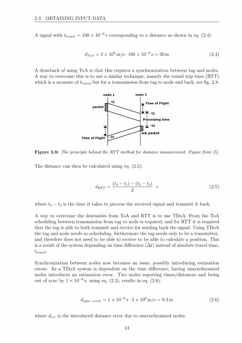
A drawback of using ToA is that this requires a synchronization between tag and nodes.A way to overcome this is to use a similar technique, namely the round trip time (RTT)which is a measure of ttravel but for a transmission from tag to node and back, see fig. 2.8.
Figure 2.8: The principle behind the RTT method for distance measurement. Figure from [5].
The distance can then be calculated using eq. (2.5):
dRTT =(t4 − t1)− (t3 − t2)
2· c (2.5)
where t3 − t2 is the time it takes to process the received signal and transmit it back.
A way to overcome the downsides from ToA and RTT is to use TDoA. From the ToAscheduling between transmission from tag to node is required, and for RTT it is requiredthat the tag is able to both transmit and receive for sending back the signal. Using TDoAthe tag and node needs no scheduling, furthermore the tag needs only to be a transmitter,and therefore does not need to be able to receive to be able to calculate a position. Thisis a result of the system depending on time difference (∆t) instead of absolute travel time,ttravel.
Synchronization between nodes now becomes an issue, possibly introducing estimationerrors. As a TDoA system is dependent on the time difference, having unsynchronizednodes introduces an estimation error. Two nodes reporting times/distances and beingout of sync by 1× 10⁻⁹ s, using eq. (2.3), results in eq. (2.6):
dsync−error = 1× 10−9 s · 3× 108 m/s = 0.3 m (2.6)
where derr is the introduced distance error due to unsynchronized nodes.
13
2.3. OBTAINING INPUT DATA
2.3.2 AoA
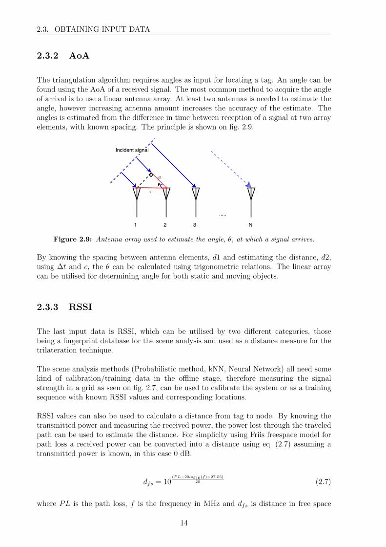
The triangulation algorithm requires angles as input for locating a tag. An angle can befound using the AoA of a received signal. The most common method to acquire the angleof arrival is to use a linear antenna array. At least two antennas is needed to estimate theangle, however increasing antenna amount increases the accuracy of the estimate. Theangles is estimated from the difference in time between reception of a signal at two arrayelements, with known spacing. The principle is shown on fig. 2.9.
Figure 2.9: Antenna array used to estimate the angle, θ, at which a signal arrives.
By knowing the spacing between antenna elements, d1 and estimating the distance, d2,using ∆t and c, the θ can be calculated using trigonometric relations. The linear arraycan be utilised for determining angle for both static and moving objects.
2.3.3 RSSI
The last input data is RSSI, which can be utilised by two different categories, thosebeing a fingerprint database for the scene analysis and used as a distance measure for thetrilateration technique.
The scene analysis methods (Probabilistic method, kNN, Neural Network) all need somekind of calibration/training data in the offline stage, therefore measuring the signalstrength in a grid as seen on fig. 2.7, can be used to calibrate the system or as a trainingsequence with known RSSI values and corresponding locations.
RSSI values can also be used to calculate a distance from tag to node. By knowing thetransmitted power and measuring the received power, the power lost through the traveledpath can be used to estimate the distance. For simplicity using Friis freespace model forpath loss a received power can be converted into a distance using eq. (2.7) assuming atransmitted power is known, in this case 0 dB.
dfs = 10(PL−20log10(f)+27.55)
20 (2.7)
where PL is the path loss, f is the frequency in MHz and dfs is distance in free space
14
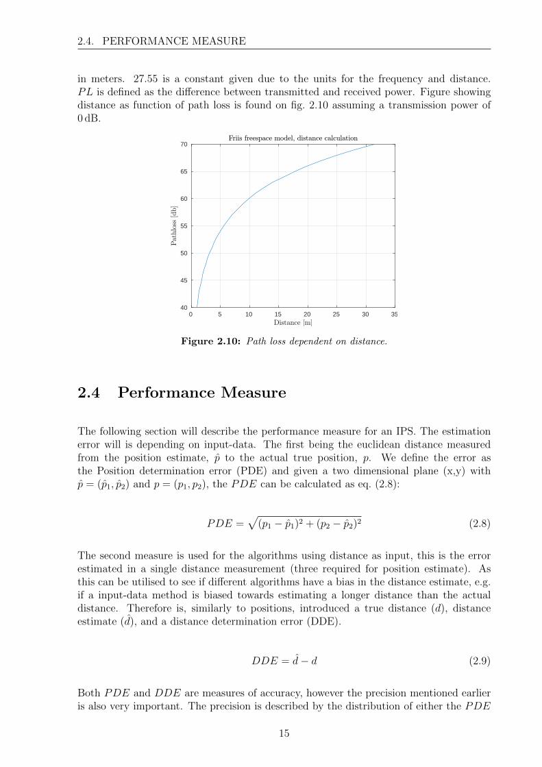
2.4. PERFORMANCE MEASURE
in meters. 27.55 is a constant given due to the units for the frequency and distance.PL is defined as the difference between transmitted and received power. Figure showingdistance as function of path loss is found on fig. 2.10 assuming a transmission power of0 dB.
0 5 10 15 20 25 30 35Distance [m]
40
45
50
55
60
65
70
Pat
hlo
ss[d
b]
Friis freespace model, distance calculation
Figure 2.10: Path loss dependent on distance.
2.4 Performance Measure
The following section will describe the performance measure for an IPS. The estimationerror will is depending on input-data. The first being the euclidean distance measuredfrom the position estimate, p to the actual true position, p. We define the error asthe Position determination error (PDE) and given a two dimensional plane (x,y) withp = (p1, p2) and p = (p1, p2), the PDE can be calculated as eq. (2.8):
PDE =√
(p1 − p1)2 + (p2 − p2)2 (2.8)
The second measure is used for the algorithms using distance as input, this is the errorestimated in a single distance measurement (three required for position estimate). Asthis can be utilised to see if different algorithms have a bias in the distance estimate, e.g.if a input-data method is biased towards estimating a longer distance than the actualdistance. Therefore is, similarly to positions, introduced a true distance (d), distanceestimate (d), and a distance determination error (DDE).
DDE = d− d (2.9)
Both PDE and DDE are measures of accuracy, however the precision mentioned earlieris also very important. The precision is described by the distribution of either the PDE
15

2.4. PERFORMANCE MEASURE
or DDE. For the following chapters, the precision will either be described in terms of thedistribution of the error source, or by the distribution of simulated or measured errors inDDE or PDE.
In practice, the impact of the environment can introduce large variations on the DDEand PDE. Both AoA, ToA and RSSI has large variations in the indoor environment andchapter 3 evaluates the performance of the different characteristics to find a target forfurther examination and evaluations.
16
Chapter 3
Simulations of Basic LocalisationMethods
The following chapter will describe the evaluation of the basic channel characteristics andthe corresponding methods which can be utilised for position determination. Simulationswill be made dependent on the fluctuations, attenuations and other system performancemetrics, which impacts the system. The performance metrics is depending on the methodinvestigated.
For some of the localisation methods, especially scene analysis, inspiration and evaluationresults were sought elsewhere.
The following sections will provide simple position estimations based on the differentlocalisation methods and channel characteristics mentioned in sections 2.2 and 2.3. Sec-tion 3.1 will investigate AoA used with triangulation, where the largest error occurs dueto the wide angular spread of the received signal. Section 3.2 examines the usage of RSSI,first in the case of fingerprinting and later as a measure of distance. The largest errorhere occurs due to fluctuations in RSSI. Following in section 3.3 will be an examinationof ToA and the performance of this. The largest error occurs due to the bandwidth of thesystem and detectability of the direct path. Section 3.4 concludes the basic simulationsand summarize the results.
The reason to investigate the basic localisation systems and the performance of these is tofind the most promising technique to further investigate for indoor localisation. Thereforeno complex or advanced assumptions or algorithms are made for the following evaluations.
3.1 AoA
Examining the angle of arrival for an IPS is a difficult task, as reality shows an AoAwhich is uniformly distributed in angle between [0;2π]. This is a result of the reflectionon surfaces in e.g. an office. Reflections are made on walls, floors, ceilings, desks, chairs,
17
3.1. AOA
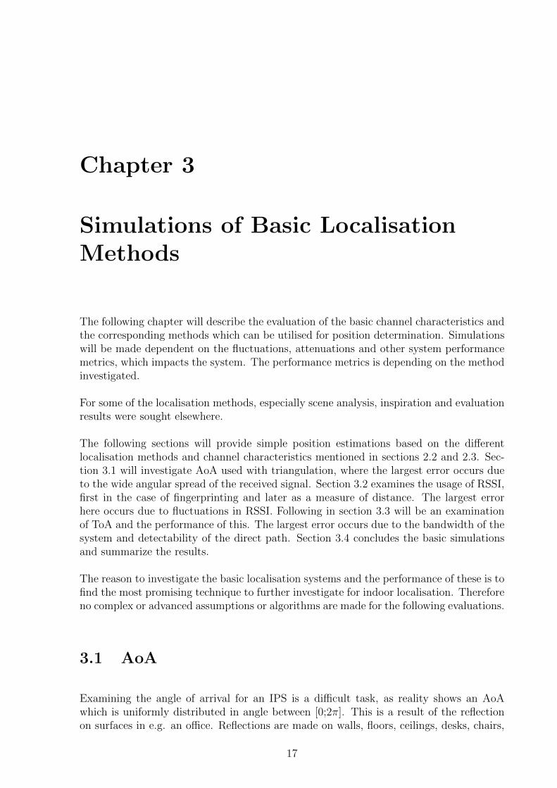
doors, etc. A raytracing sketch is found on fig. 3.1.
Figure 3.1: Sketch of an example of isotropic radiating transmitter and the reception at thereceiver. Figure from [8].
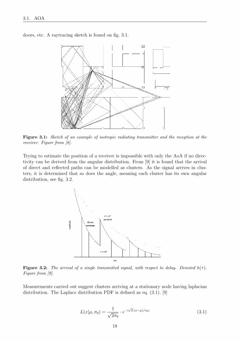
Trying to estimate the position of a receiver is impossible with only the AoA if no direc-tivity can be derived from the angular distribution. From [9] it is found that the arrivalof direct and reflected paths can be modelled as clusters. As the signal arrives in clus-ters, it is determined that so does the angle, meaning each cluster has its own angulardistribution, see fig. 3.2.
Figure 3.2: The arrival of a single transmitted signal, with respect to delay. Denoted h(τ).Figure from [9].
Measurements carried out suggest clusters arriving at a stationary node having laplaciandistribution. The Laplace distribution PDF is defined as eq. (3.1). [9]
L(x|µ, σθ) =1√2σθ· e−|
√2·(x−µ)/σθ| (3.1)
18
3.1. AOA
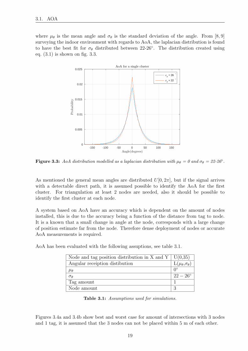
where µθ is the mean angle and σθ is the standard deviation of the angle. From [8, 9]surveying the indoor environment with regards to AoA, the laplacian distribution is foundto have the best fit for σθ distributed between 22-26◦. The distribution created usingeq. (3.1) is shown on fig. 3.3.
-150 -100 -50 0 50 100 150Angle(degrees)
0
0.005
0.01
0.015
0.02
0.025Probab
ility
AoA for a single cluster
σθ = 26 °
σθ = 22 °
Figure 3.3: AoA distribution modelled as a laplacian distribution with µθ = 0 and σθ = 22-26◦.
As mentioned the general mean angles are distributed U [0, 2π], but if the signal arriveswith a detectable direct path, it is assumed possible to identify the AoA for the firstcluster. For triangulation at least 2 nodes are needed, also it should be possible toidentify the first cluster at each node.
A system based on AoA have an accuracy which is dependent on the amount of nodesinstalled, this is due to the accuracy being a function of the distance from tag to node.It is a known that a small change in angle at the node, corresponds with a large changeof position estimate far from the node. Therefore dense deployment of nodes or accurateAoA measurements is required.
AoA has been evaluated with the following assuptions, see table 3.1.
Node and tag position distribution in X and Y U(0,35)Angular receiption distibution L(µθ,σθ)µθ 0◦
σθ 22− 26◦
Tag amount 1Node amount 3
Table 3.1: Assumptions used for simulations.
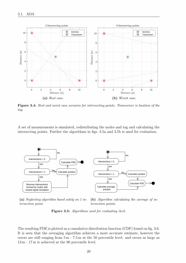
Figures 3.4a and 3.4b show best and worst case for amount of intersections with 3 nodesand 1 tag, it is assumed that the 3 nodes can not be placed within 5 m of each other.
19
3.1. AOA
0 2 4 6 8 10Distance [m]
0
2
4
6
8
10
Dista
nce
[m]
3 Intersecting points
AnchorsTransceiver
(a) Best case.
0 2 4 6 8 10Distance [m]
0
2
4
6
8
10
Dista
nce
[m]
0 Intersecting points
AnchorsTransceiver
(b) Worst case.
Figure 3.4: Best and worst case scenario for intersecting points. Transceiver is location of thetag.
A set of measurements is simulated, redistributing the nodes and tag and calculating theintersecting points. Further the algorithms in figs. 3.5a and 3.5b is used for evaluation.
Calculate PDE
yes
No
yes
No
Remove intersections formed by nodes with
lowest signal receiption
Calculate positionintersections > 1
intersections > 0
(a) Neglecting algorithm based solely on 1 in-tersection point.
Calculate PDE
yes
No
yes
No
Calculate average position
Calculate positionintersections > 1
intersections > 0
(b) Algorithm calculating the average of in-tersection points.
Figure 3.5: Algorithms used for evaluating AoA.
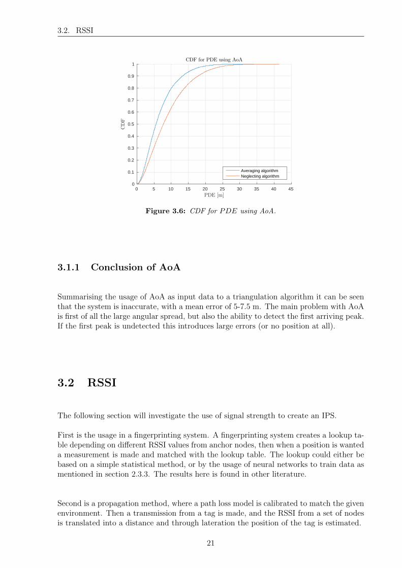
The resulting PDE is plotted as a cumulative distribution function (CDF) found on fig. 3.6.It is seen that the averaging algorithm achieves a more accurate estimate, however theerrors are still ranging from 5 m - 7.5 m at the 50 percentile level. and errors as large as13 m - 17 m is achieved at the 90 percentile level.
20
3.2. RSSI
0 5 10 15 20 25 30 35 40 45PDE [m]
0
0.1
0.2
0.3
0.4
0.5
0.6
0.7
0.8
0.9
1
CDF
CDF for PDE using AoA
Averaging algorithmNeglecting algorithm
Figure 3.6: CDF for PDE using AoA.
3.1.1 Conclusion of AoA
Summarising the usage of AoA as input data to a triangulation algorithm it can be seenthat the system is inaccurate, with a mean error of 5-7.5 m. The main problem with AoAis first of all the large angular spread, but also the ability to detect the first arriving peak.If the first peak is undetected this introduces large errors (or no position at all).
3.2 RSSI
The following section will investigate the use of signal strength to create an IPS.
First is the usage in a fingerprinting system. A fingerprinting system creates a lookup ta-ble depending on different RSSI values from anchor nodes, then when a position is wanteda measurement is made and matched with the lookup table. The lookup could either bebased on a simple statistical method, or by the usage of neural networks to train data asmentioned in section 2.3.3. The results here is found in other literature.
Second is a propagation method, where a path loss model is calibrated to match the givenenvironment. Then a transmission from a tag is made, and the RSSI from a set of nodesis translated into a distance and through lateration the position of the tag is estimated.
21
3.2. RSSI
3.2.1 Fingerprinting
For the accuracy of a fingerprinting system, inspiration and results in other literature hasbeen found, as implementation and testing of such system would require much time, alsothe precision of fingerprinting systems differs a lot depending on the individual systemand setup area.
Examining the fingerprinting based method, the accuracy in these systems depends mostlyon the amount of nodes and the resolution of the fingerprinting grid, together with thefingerprinting algorithm.
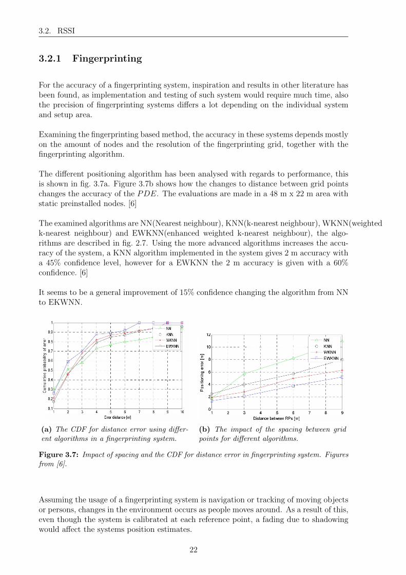
The different positioning algorithm has been analysed with regards to performance, thisis shown in fig. 3.7a. Figure 3.7b shows how the changes to distance between grid pointschanges the accuracy of the PDE. The evaluations are made in a 48 m x 22 m area withstatic preinstalled nodes. [6]
The examined algorithms are NN(Nearest neighbour), KNN(k-nearest neighbour), WKNN(weightedk-nearest neighbour) and EWKNN(enhanced weighted k-nearest neighbour), the algo-rithms are described in fig. 2.7. Using the more advanced algorithms increases the accu-racy of the system, a KNN algorithm implemented in the system gives 2 m accuracy witha 45% confidence level, however for a EWKNN the 2 m accuracy is given with a 60%confidence. [6]
It seems to be a general improvement of 15% confidence changing the algorithm from NNto EKWNN.
(a) The CDF for distance error using differ-ent algorithms in a fingerprinting system.
(b) The impact of the spacing between gridpoints for different algorithms.
Figure 3.7: Impact of spacing and the CDF for distance error in fingerprinting system. Figuresfrom [6].
Assuming the usage of a fingerprinting system is navigation or tracking of moving objectsor persons, changes in the environment occurs as people moves around. As a result of this,even though the system is calibrated at each reference point, a fading due to shadowingwould affect the systems position estimates.
22
3.2. RSSI
3.2.2 Distance Propagation Method
In the following section the accuracy of a distance propagation method will be investigated.Generally a propagation based method is inaccurate compared with a fingerprinting sys-tem, which often is a result of shadow fading in an indoor environment. The impact of theshadow effects are lowered in a fingerprinting system as the calibration procedure takesinto account the attenuation of walls, roofs and other stationary attenuating objects.
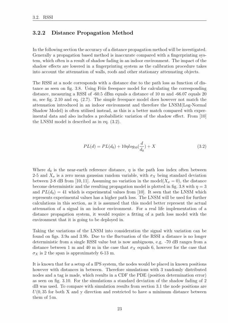
The RSSI at a node corresponds with a distance due to the path loss as function of dis-tance as seen on fig. 3.8. Using Friis freespace model for calculating the correspondingdistance, measuring a RSSI of -60.5 dBm equals a distance of 10 m and -66.07 equals 20m, see fig. 2.10 and eq. (2.7). The simple freespace model does however not match theattenuation introduced in an indoor environment and therefore the LNSM(Log-NormalShadow Model) is often utilised instead, as this is a better match compared with exper-imental data and also includes a probabilistic variation of the shadow effect. From [10]the LNSM model is described as in eq. (3.2).
PL(d) = PL(d0) + 10ηlog10(d
d0
) +X (3.2)
Where d0 is the near-earth reference distance, η is the path loss index often between2-5 and Xσ is a zero mean gaussian random variable, with σX being standard deviationbetween 2-8 dB from [10,11]. Assuming no variation in the model(Xσ = 0), the distancebecome deterministic and the resulting propagation model is plotted in fig. 3.8 with η = 3and PL(d0) = 41 which is experimental values from [10]. It seen that the LNSM whichrepresents experimental values has a higher path loss. The LNSM will be used for furthercalculations in this section, as it is assumed that this model better represent the actualattenuation of a signal in an indoor environment. For a real life implementation of adistance propagation system, it would require a fitting of a path loss model with theenvironment that it is going to be deployed in.
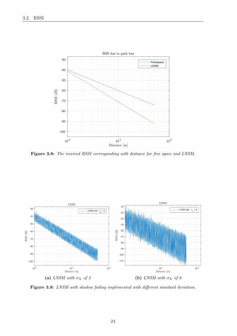
Taking the variations of the LNSM into consideration the signal with variation can befound on figs. 3.9a and 3.9b. Due to the fluctuation of the RSSI a distance is no longerdeterministic from a single RSSI value but is now ambiguous, e.g. -70 dB ranges from adistance between 1 m and 40 m in the case that σX equals 6, however for the case thatσX is 2 the span is approximately 6-13 m.
It is known that for a setup of a IPS system, the nodes would be placed in known positionshowever with distances in between. Therefore simulations with 3 randomly distributednodes and a tag is made, which results in a CDF the PDE (position determination error)as seen on fig. 3.10. For the simulations a standard deviation of the shadow fading of 2dB was used. To compare with simulation results from section 3.1 the node positions areU(0, 35 for both X and y direction and restricted to have a minimum distance betweenthem of 5 m.
23
3.2. RSSI
10 0 10 1 10 2
Distance [m]
-100
-90
-80
-70
-60
-50
-40
-30RSSI[d
B]
RSS due to path loss
FreespaceLNSM
Figure 3.8: The received RSSI corresponding with distance for free space and LNSM.
10 0 10 1 10 2
Distance [m]
-100
-90
-80
-70
-60
-50
-40
-30
RSSI[d
B]
LNSM
LNSM with <X
= 2
(a) LNSM with σX of 2
10 1 10 2
Distance [m]
-110
-100
-90
-80
-70
-60
-50
-40
-30
-20
RSSI[d
B]
LNSM
LNSM with <X
= 6
(b) LNSM with σX of 6
Figure 3.9: LNSM with shadow fading implemented with different standard deviation.
24
3.3. TOA
0 5 10 15 20 25 30 35Distance error[m]
0
0.1
0.2
0.3
0.4
0.5
0.6
0.7
0.8
0.9
1
CD
F
CDF for distance error using uniformly distributed anchor nodes
3 Anchors: Averaging algorithm
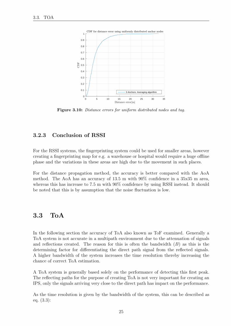
Figure 3.10: Distance errors for uniform distributed nodes and tag.
3.2.3 Conclusion of RSSI
For the RSSI systems, the fingerprinting system could be used for smaller areas, howevercreating a fingerprinting map for e.g. a warehouse or hospital would require a huge offlinephase and the variations in these areas are high due to the movement in such places.
For the distance propagation method, the accuracy is better compared with the AoAmethod. The AoA has an accuracy of 13.5 m with 90% confidence in a 35x35 m area,whereas this has increase to 7.5 m with 90% confidence by using RSSI instead. It shouldbe noted that this is by assumption that the noise fluctuation is low.
3.3 ToA
In the following section the accuracy of ToA also known as ToF examined. Generally aToA system is not accurate in a multipath environment due to the attenuation of signalsand reflections created. The reason for this is often the bandwidth (B) as this is thedetermining factor for differentiating the direct path signal from the reflected signals.A higher bandwidth of the system increases the time resolution thereby increasing thechance of correct ToA estimation.
A ToA system is generally based solely on the performance of detecting this first peak.The reflecting paths for the purpose of creating ToA is not very important for creating anIPS, only the signals arriving very close to the direct path has impact on the performance.
As the time resolution is given by the bandwidth of the system, this can be described aseq. (3.3):
25
3.3. TOA
Tres =1
B(3.3)
Generally in a system estimation of ToA can’t be obtained more precise than what isallowed by the system bandwidth.
The reflections can be seen as a set of sinc-functions with different time-delays and com-plex weights, as mentioned in appendix B. It should be noted that the sinc-function occurswhen a rectangular window is used to convert the frequency domain data to time domainimpulse response. Using a hamming window instead the pulse shape would be a raisedcosine, as the sidelobes are suppressed. Having a large bandwidth allows for these pulseshapes to be narrower, thereby allowing for easier differentiation between the differentpaths. By having B = ∞ the pulse shapes converges to a dirac pulses and the exacttime-delay can be found.
As B = ∞ is not possible to obtain, the received signal will be a sum of the pulses atdifferent time-delays.
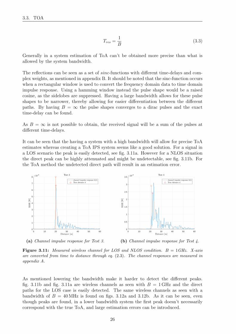
It can be seen that the having a system with a high bandwidth will allow for precise ToAestimates whereas creating a ToA IPS system seems like a good solution. For a signal ina LOS scenario the peak is easily detected, see fig. 3.11a. However for a NLOS situationthe direct peak can be highly attenuated and might be undetectable, see fig. 3.11b. Forthe ToA method the undetected direct path will result in an estimation error.
0 10 20 30 40 50 600
1
2
3
4
5
6
7
810-4
(a) Channel impulse response for Test 3.
0 10 20 30 40 50 600
0.5
1
1.5
2
2.5
3
3.510-4
(b) Channel impulse response for Test 4.
Figure 3.11: Measured wireless channel for LOS and NLOS condition. B = 1GHz. X-axisare converted from time to distance through eq. (2.3). The channel responses are measured inappendix A.
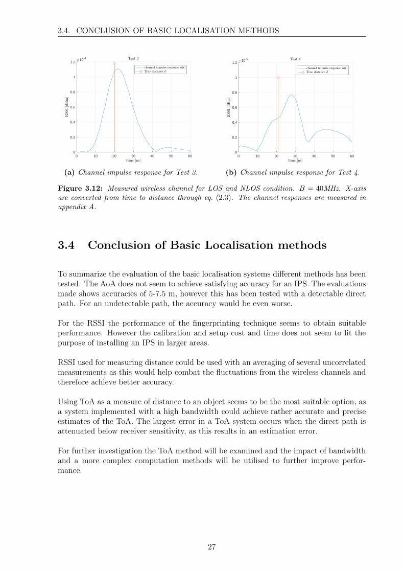
As mentioned lowering the bandwidth make it harder to detect the different peaks.fig. 3.11b and fig. 3.11a are wireless channels as seen with B = 1 GHz and the directpaths for the LOS case is easily detected. The same wireless channels as seen with abandwidth of B = 40 MHz is found on figs. 3.12a and 3.12b. As it can be seen, eventhough peaks are found, in a lower bandwidth system the first peak doesn’t necessarilycorrespond with the true ToA, and large estimation errors can be introduced.
26
3.4. CONCLUSION OF BASIC LOCALISATION METHODS
0 10 20 30 40 50 600
0.2
0.4
0.6
0.8
1
1.210-4
(a) Channel impulse response for Test 3.
0 10 20 30 40 50 600
0.2
0.4
0.6
0.8
1
1.210-5
(b) Channel impulse response for Test 4.
Figure 3.12: Measured wireless channel for LOS and NLOS condition. B = 40MHz. X-axisare converted from time to distance through eq. (2.3). The channel responses are measured inappendix A.
3.4 Conclusion of Basic Localisation methods
To summarize the evaluation of the basic localisation systems different methods has beentested. The AoA does not seem to achieve satisfying accuracy for an IPS. The evaluationsmade shows accuracies of 5-7.5 m, however this has been tested with a detectable directpath. For an undetectable path, the accuracy would be even worse.
For the RSSI the performance of the fingerprinting technique seems to obtain suitableperformance. However the calibration and setup cost and time does not seem to fit thepurpose of installing an IPS in larger areas.
RSSI used for measuring distance could be used with an averaging of several uncorrelatedmeasurements as this would help combat the fluctuations from the wireless channels andtherefore achieve better accuracy.
Using ToA as a measure of distance to an object seems to be the most suitable option, asa system implemented with a high bandwidth could achieve rather accurate and preciseestimates of the ToA. The largest error in a ToA system occurs when the direct path isattenuated below receiver sensitivity, as this results in an estimation error.
For further investigation the ToA method will be examined and the impact of bandwidthand a more complex computation methods will be utilised to further improve perfor-mance.
27

Chapter 4
ToA Positioning with TimeResolution Enhancement
The following chapter will describe the investigation of a more complex ToA algorithm tofurther improve the ToA detection when using lower bandwidth systems. This is a resultof the ToA concluded the most promising technique in chapter 3.
From the further investigation of enhancing the ToA system, it is seen in several articles[12–15], that the eigenvalue decomposition (EVD) method seems like a good candidatefor developing a high-accuracy IPS. EVD is utilised in a set of different algorithms, fromthese the MUltiple SIgnal Classification (MUSIC) algorithm is used.
The chapter will consist of two parts, in sections 4.1 to 4.6 is a description of a systemmodel for a transmitter and receiver system. Following in section 4.7 is a description ofthe MUSIC algorithm.
4.1 I/Q baseband description
The system will only be described using the equivalent baseband signal. For describing atransmitted sequence such as data or pseudo random noise (PRN) the signal can be de-scribed by its amplitude and phase or by the baseband signal in terms of the mathematicalrepresentation of I/Q. I and Q are respectively the in-phase and quadrature componentof a signal.
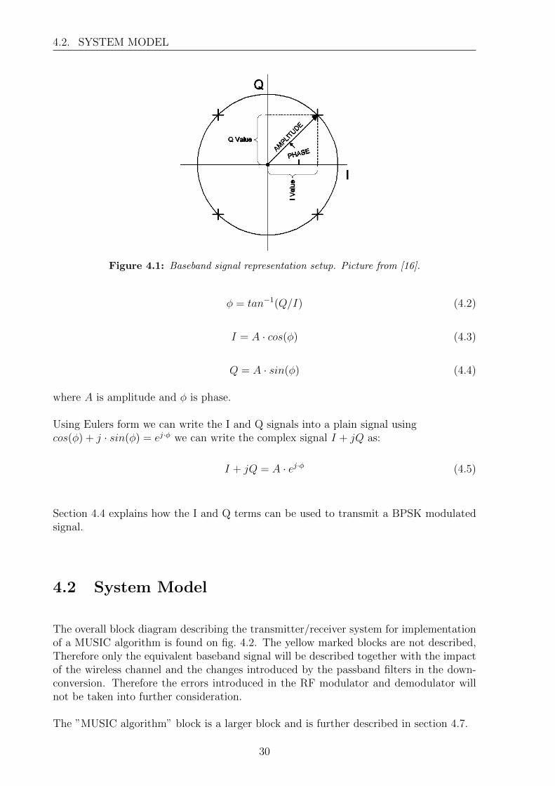
The structure of the I/Q baseband signal can be found from the amplitude and phase ofthe signals as found on fig. 4.1.
Using simple trigonometric properties, the following equations can be constructed:
A =√|I2 +Q2| (4.1)
29
4.2. SYSTEM MODEL
Figure 4.1: Baseband signal representation setup. Picture from [16].
φ = tan−1(Q/I) (4.2)
I = A · cos(φ) (4.3)
Q = A · sin(φ) (4.4)
where A is amplitude and φ is phase.
Using Eulers form we can write the I and Q signals into a plain signal usingcos(φ) + j · sin(φ) = ej·φ we can write the complex signal I + jQ as:
I + jQ = A · ej·φ (4.5)
Section 4.4 explains how the I and Q terms can be used to transmit a BPSK modulatedsignal.
4.2 System Model
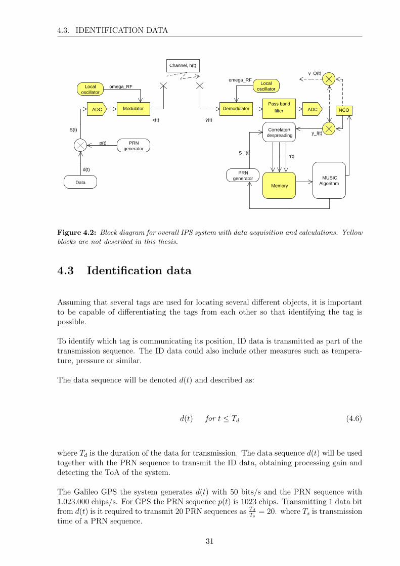
The overall block diagram describing the transmitter/receiver system for implementationof a MUSIC algorithm is found on fig. 4.2. The yellow marked blocks are not described,Therefore only the equivalent baseband signal will be described together with the impactof the wireless channel and the changes introduced by the passband filters in the down-conversion. Therefore the errors introduced in the RF modulator and demodulator willnot be taken into further consideration.
The ”MUSIC algorithm” block is a larger block and is further described in section 4.7.
30
4.3. IDENTIFICATION DATA
r(t)S_I(t)
y_Q(t)
y_I(t)
omega_RF
ý(t)x(t)
omega_RF
p(t)
S(t)
d(t)
Channel, h(t)
ADC
PRN generator
Data
Modulator
Localoscillator
MUSICAlgorithmMemory
PRN generator
Correlator/despreading
NCOADCPass band
filterDemodulator
Localoscillator
Figure 4.2: Block diagram for overall IPS system with data acquisition and calculations. Yellowblocks are not described in this thesis.
4.3 Identification data
Assuming that several tags are used for locating several different objects, it is importantto be capable of differentiating the tags from each other so that identifying the tag ispossible.
To identify which tag is communicating its position, ID data is transmitted as part of thetransmission sequence. The ID data could also include other measures such as tempera-ture, pressure or similar.
The data sequence will be denoted d(t) and described as:
d(t) for t ≤ Td (4.6)
where Td is the duration of the data for transmission. The data sequence d(t) will be usedtogether with the PRN sequence to transmit the ID data, obtaining processing gain anddetecting the ToA of the system.
The Galileo GPS the system generates d(t) with 50 bits/s and the PRN sequence with1.023.000 chips/s. For GPS the PRN sequence p(t) is 1023 chips. Transmitting 1 data bitfrom d(t) is it required to transmit 20 PRN sequences as Td
Ts= 20. where Ts is transmission
time of a PRN sequence.
31
4.4. GOLD CODE PRN SEQUENCE
4.4 Gold Code PRN Sequence
For transmitting the data d(t) and to obtain an estimate of the wireless channel a PRNsequence is utilised for making direct sequence spread spectrum (DSSS) transmission.
The idea is to transmit the data d(t) with a given bandwidth Bd over a much largerbandwidth Bp given by the PRN sequence p(t). This introduces a so called spread-ing/processing gain, GP , which allows for longer transmission ranges compared with justtransmission of the data directly onto the carrier.
GP =Bp
Bd
(4.7)
where Bp is the bandwidth of the PRN sequence and Bd is the bandwidth of the IDdata [17].
The PRN code p(t) can be seen as a sequence of chips c(t).
c(t) is defined as eq. (4.8):
c(t) =
{1, for − Tc/2 < t < Tc/2 ,
0, Otherwise(4.8)
where TC is duration of a single chip.
Using the chip time c(t), the PRN sequence p(t) is given by eq. (4.9)
p(t) =
N∑i=0
c(t− i · Tc − Tc/2) for 0 < t < Ts (4.9)
Where TS = N · Tc and N is amount of chips.
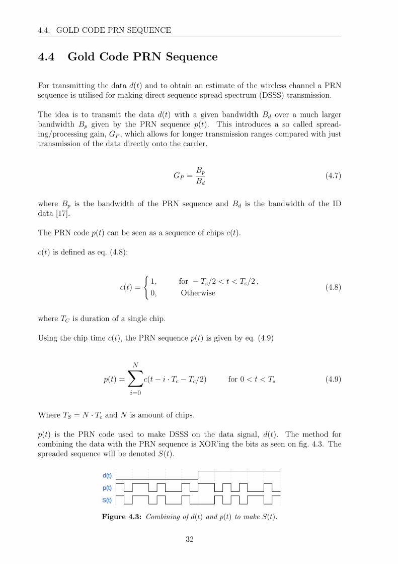
p(t) is the PRN code used to make DSSS on the data signal, d(t). The method forcombining the data with the PRN sequence is XOR’ing the bits as seen on fig. 4.3. Thespreaded sequence will be denoted S(t).
Figure 4.3: Combining of d(t) and p(t) to make S(t).
32
4.4. GOLD CODE PRN SEQUENCE
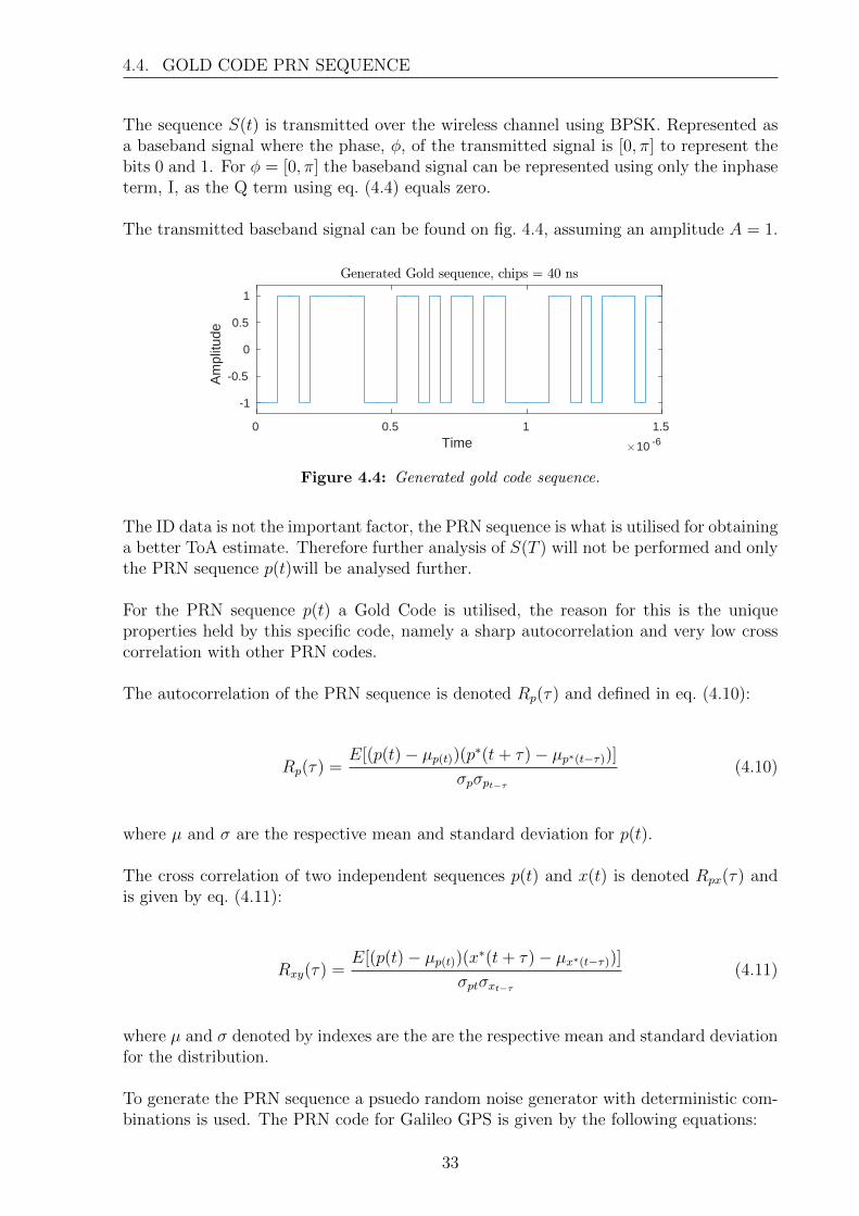
The sequence S(t) is transmitted over the wireless channel using BPSK. Represented asa baseband signal where the phase, φ, of the transmitted signal is [0, π] to represent thebits 0 and 1. For φ = [0, π] the baseband signal can be represented using only the inphaseterm, I, as the Q term using eq. (4.4) equals zero.
The transmitted baseband signal can be found on fig. 4.4, assuming an amplitude A = 1.
0 0.5 1 1.5Time
×10 -6
-1
-0.5
0
0.5
1
Am
plitu
de
Generated Gold sequence, chips = 40 ns
Figure 4.4: Generated gold code sequence.
The ID data is not the important factor, the PRN sequence is what is utilised for obtaininga better ToA estimate. Therefore further analysis of S(T ) will not be performed and onlythe PRN sequence p(t)will be analysed further.
For the PRN sequence p(t) a Gold Code is utilised, the reason for this is the uniqueproperties held by this specific code, namely a sharp autocorrelation and very low crosscorrelation with other PRN codes.
The autocorrelation of the PRN sequence is denoted Rp(τ) and defined in eq. (4.10):
Rp(τ) =E[(p(t)− µp(t))(p∗(t+ τ)− µp∗(t−τ))]
σpσpt−τ(4.10)
where µ and σ are the respective mean and standard deviation for p(t).
The cross correlation of two independent sequences p(t) and x(t) is denoted Rpx(τ) andis given by eq. (4.11):
Rxy(τ) =E[(p(t)− µp(t))(x∗(t+ τ)− µx∗(t−τ))]
σptσxt−τ(4.11)
where µ and σ denoted by indexes are the are the respective mean and standard deviationfor the distribution.
To generate the PRN sequence a psuedo random noise generator with deterministic com-binations is used. The PRN code for Galileo GPS is given by the following equations:
33
4.4. GOLD CODE PRN SEQUENCE
P1 = 1 + x3 + x10 (4.12)
P2 = 1 + x2 + x3 + x6 + x8 + x9 + x10 (4.13)
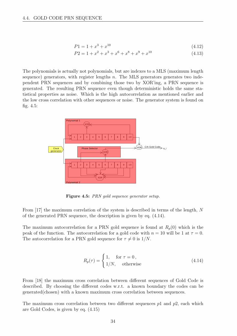
The polynomials is actually not polynomials, but are indexes to a MLS (maximum lengthsequence) generators, with register lengths n. The MLS generators generates two inde-pendent PRN sequences and by combining those two by XOR’ing, a PRN sequence isgenerated. The resulting PRN sequence even though deterministic holds the same sta-tistical properties as noise. Which is the high autocorrelation as mentioned earlier andthe low cross correlation with other sequences or noise. The generator system is found onfig. 4.5:
1 2 3 4 5 6 7 8 9 1 0
XOR
1 2 3 4 5 6 7 8 9 1 0
XOR
XOR C/A Gold Code
XOR
Phase SelectorClock generator
Polynomial 1
Polynomial 2
a_i
Figure 4.5: PRN gold sequence generator setup.
From [17] the maximum correlation of the system is described in terms of the length, Nof the generated PRN sequence, the description is given by eq. (4.14).
The maximum autocorrelation for a PRN gold sequence is found at Rp(0) which is thepeak of the function. The autocorrelation for a gold code with n = 10 will be 1 at τ = 0.The autocorrelation for a PRN gold sequence for τ 6= 0 is 1/N .
Rp(τ) =
{1, for τ = 0 ,
1/N, otherwise(4.14)
From [18] the maximum cross correlation between different sequences of Gold Code isdescribed. By choosing the different codes w.r.t. a known boundary the codes can begenerated(chosen) with a known maximum cross correlation between sequences.
The maximum cross correlation between two different sequences p1 and p2, each whichare Gold Codes, is given by eq. (4.15)
34
4.4. GOLD CODE PRN SEQUENCE
|RS1,S2| ≤
2(n+1)/2 + 1
N, for n odd ,
2(n+2)/2 + 1
N, for n even
(4.15)
where n is the amount of bits in the MLS generator and N is the total length of thesequence.
Given the Gold code used for GPS satellites, and a MLS generator with n = 10, themaximum theoretical cross correlation for two different PRN sequences is:
|Rp1,p2| ≤2(10+2)/2 + 1
1023= 65/1023 ≈ 0.064 (4.16)
The receiver for a system utilising Gold Code searches to maximize the cross correlationbetween the received signal and a replicated gold code sequence at the receiver node.
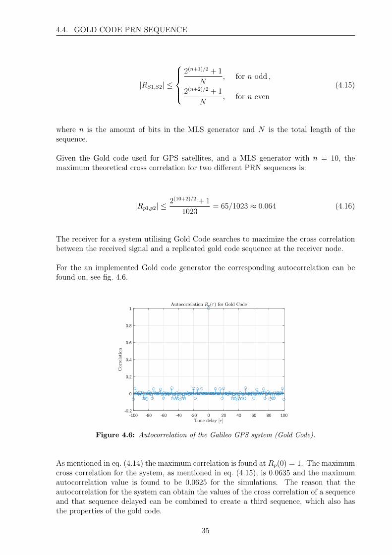
For the an implemented Gold code generator the corresponding autocorrelation can befound on, see fig. 4.6.
-100 -80 -60 -40 -20 0 20 40 60 80 100-0.2
0
0.2
0.4
0.6
0.8
1
Figure 4.6: Autocorrelation of the Galileo GPS system (Gold Code).
As mentioned in eq. (4.14) the maximum correlation is found at Rp(0) = 1. The maximumcross correlation for the system, as mentioned in eq. (4.15), is 0.0635 and the maximumautocorrelation value is found to be 0.0625 for the simulations. The reason that theautocorrelation for the system can obtain the values of the cross correlation of a sequenceand that sequence delayed can be combined to create a third sequence, which also hasthe properties of the gold code.
35
4.5. CHANNEL
4.5 Channel
The transmitted sequence p(t) is sent over a wireless channel. The wireless channel willbe described by the use of a multi path environment model with uncorrelated scattersin both time and frequency domain. The reason for uncorrelated scatters is that eachreflected path due to e.g. tables, walls, chairs, windows and similar, are independent.Therefore the channel h(t) can be described as a sum of K paths each path i with its ownattenuation αi, phase shift φi and time-delay τi. The model is described in eq. (4.17):
h(t) =
K−1∑i=0
αi · ejφiδ(t− τi) (4.17)
The channel described by its I/Q terms can be seen on eq. (4.18).
h(t) = hI(t) + j · hQ(t) (4.18)
Using the PRN-sequence description from fig. 4.3 with the corresponding I/Q term, thetransmission of p(t) over the wireless channel is a complex convolution of h(t) and p(t).Denote the received signal r(t) this can be described by eqs. (4.19) to (4.21):
r(t) = p(t) ∗ h(t) + w(t) (4.19)
= (pI(t) + j · pQ(t)) ∗ (hI(t) + j · hQ(t)) + w(t) (4.20)
= pI(t) ∗ pI(t) + pI(t) ∗ j · hQ(t) + j · pQ(t) ∗ hI(t) + pQ(t) ∗ hI(t) + w(t) (4.21)
Where w(t) is additive white gaussion noise (AWGN).
Using the BPSK transmission the quadrature component for p(t) equals zero and theabove reduces to eq. (4.22):
r(t) = pI(t) ∗ h(t) + w(t) (4.22)
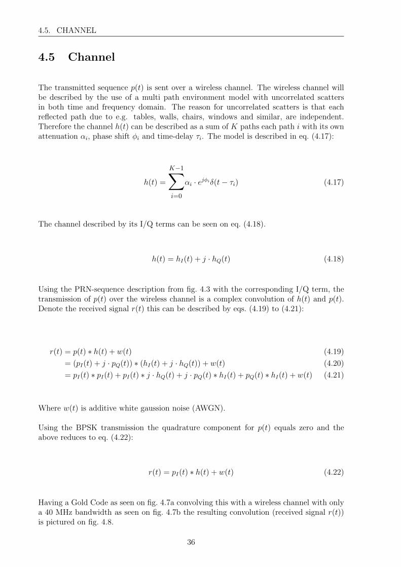
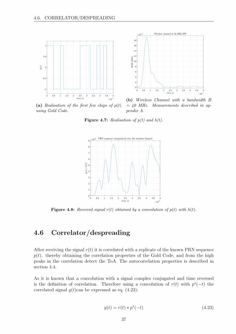
Having a Gold Code as seen on fig. 4.7a convolving this with a wireless channel with onlya 40 MHz bandwidth as seen on fig. 4.7b the resulting convolution (received signal r(t))is pictured on fig. 4.8.
36
4.6. CORRELATOR/DESPREADING
0 0.5 1 1.5 2 2.5 3 3.5 4 4.5 5
10-7
-1
-0.5
0
0.5
1
(a) Realisation of the first few chips of p(t)using Gold Code.
0 0.5 1 1.5 2 2.5 3 3.5 4 4.5 5
10-7
0
2
4
6
8
10
12
14
16
18
10-6
(b) Wireless Channel with a bandwidth B= 40 MHz. Measurements described in ap-pendix A.
Figure 4.7: Realisation of p(t) and h(t).
0 0.5 1 1.5 2 2.5 3 3.5 4 4.5 5
10-7
0
1
2
3
4
5
6
7
8
910-5
Figure 4.8: Received signal r(t) obtained by a convolution of p(t) with h(t).
4.6 Correlator/despreading
After receiving the signal r(t) it is correlated with a replicate of the known PRN sequencep(t). thereby obtaining the correlation properties of the Gold Code, and from the highpeaks in the correlation detect the ToA. The autocorrelation properties is described insection 4.4.
As it is known that a convolution with a signal complex conjugated and time reversedis the definition of correlation. Therefore using a convolution of r(t) with p∗(−t) thecorrelated signal y(t)can be expressed as eq. (4.23):
y(t) = r(t) ∗ p∗(−t) (4.23)
37

4.6. CORRELATOR/DESPREADING
Which can be rewritten as eq. (4.24):
y(t) = Rp(τ) ∗ h(t) + w(t) (4.24)
It is now seen that y(t) is expressed as the autocorrelation of the sequence p(t) convolvedwith h(t). The signal y(t) is shown on fig. 4.9a, this is found by correlating the channelfound on fig. 4.8 with a time shifted version of the intial transmitted prn sequence p(t).This is plotted together with the autocorrelation for that specific PRN code Rp(τ). Fromfig. 4.9b is is easily seen that the the autocorrelation is time shifted by a delay τ , in thiscase approximately 75 ns corresponding with a distance of 22.5 m.
-3 -2 -1 0 1 2 3
10-5
0
0.1
0.2
0.3
0.4
0.5
0.6
0.7
0.8
0.9
1
(a) y(t) and Rp(τ) plotted.
-2 -1.5 -1 -0.5 0 0.5 1 1.5 2
10-7
-0.2
0
0.2
0.4
0.6
0.8
1
1.2
(b) Zoomed on maximum correlation area.
Figure 4.9: Search method for first path delay.
The method for finding the delay which represents the direct path is by using severalshifted cross correlators at the receiver. The cross correlator obtaining the highest corre-lation level will be chosen as the first arriving peak.
This can be seen as a sweep of RP (τ) over the received signal y(t) to find the maximumcorrelation. The timeshift yielding the maximum correlation is chosen as the delay τ0 (firstpath signal). For further description of this cross correlation receiver (RAKE receiver),see [19].
Calculating the maximum of the average of a series of autocorrelation function, it ispossible to determine the maximum of these as seen on fig. 4.9b. The series of differentautocorrelations utilised for averaging is found on fig. 4.10a, together with the averagemarked as the black line and the true distance marked with a red stem. The error foundby using this method in different SNR-levels is seen on fig. 4.10b.
38
4.7. MUSIC ALGORITHM
0 0.5 1 1.5 2 2.5
10-7
0
0.5
1
1.5
2
2.5
10-5
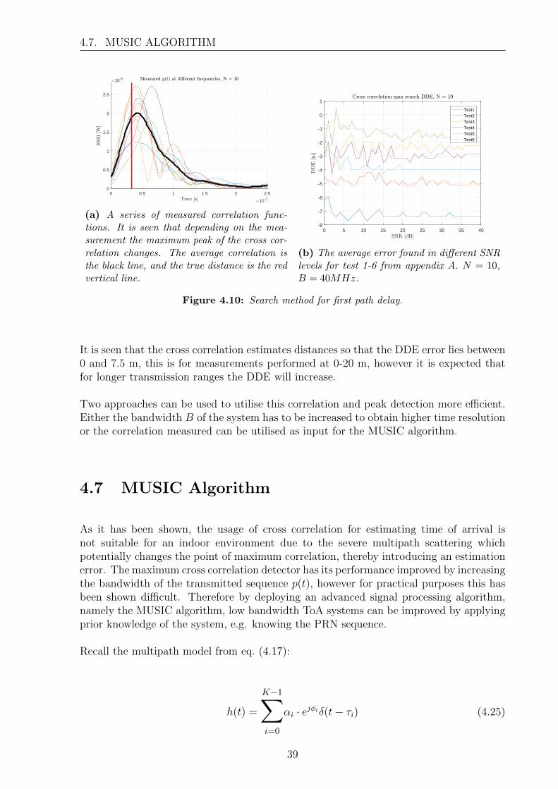
(a) A series of measured correlation func-tions. It is seen that depending on the mea-surement the maximum peak of the cross cor-relation changes. The average correlation isthe black line, and the true distance is the redvertical line.
0 5 10 15 20 25 30 35 40-8
-7
-6
-5
-4
-3
-2
-1
0
1
Test1Test2Test3Test4Test5Test6
(b) The average error found in different SNRlevels for test 1-6 from appendix A. N = 10,B = 40MHz.
Figure 4.10: Search method for first path delay.
It is seen that the cross correlation estimates distances so that the DDE error lies between0 and 7.5 m, this is for measurements performed at 0-20 m, however it is expected thatfor longer transmission ranges the DDE will increase.
Two approaches can be used to utilise this correlation and peak detection more efficient.Either the bandwidth B of the system has to be increased to obtain higher time resolutionor the correlation measured can be utilised as input for the MUSIC algorithm.
4.7 MUSIC Algorithm
As it has been shown, the usage of cross correlation for estimating time of arrival isnot suitable for an indoor environment due to the severe multipath scattering whichpotentially changes the point of maximum correlation, thereby introducing an estimationerror. The maximum cross correlation detector has its performance improved by increasingthe bandwidth of the transmitted sequence p(t), however for practical purposes this hasbeen shown difficult. Therefore by deploying an advanced signal processing algorithm,namely the MUSIC algorithm, low bandwidth ToA systems can be improved by applyingprior knowledge of the system, e.g. knowing the PRN sequence.
Recall the multipath model from eq. (4.17):
h(t) =
K−1∑i=0
αi · ejφiδ(t− τi) (4.25)
39
4.7. MUSIC ALGORITHM
where K − 1 is the amount of multipath scatters, αi is the attenuation, φi is the phaseand τi is the propagation delay.
To use the music algorithm a model has to be established fist. A linear combination ofautocorrelation functions can be utilised to describe the received signal y.
The following model and vector notation from [20] will be used:
y = A · u+ w (4.26)
where
y =[y(0) y(1) · · · y(K − 1)
]T(4.27)
A =[RP (τ0) RP (τ1) · · · RP (τK−1)
]T(4.28)
u =[u0 u1 · · · uK−1
](4.29)
w =[w(0) w(1) · · · w(K − 1)
]T(4.30)
(4.31)
where u is the complex weights αi · ejφi from the channel eq. (4.25) and RP (τ) is theautocorrelation of the PRN sequence shifted by τ . w is additive white noise.
The MUSIC algorithm is as mentioned earlier based on the eigenvalue decomposition ofthe covariance matrix of the autocorrelation functions described by eq. (4.26). From [19]the input covariance matrix for the MUSIC algorithm is described as eq. (4.32):
C = E[yy∗] (4.32)
which by inserting eq. (4.26) results in eqs. (4.33) and (4.34).
C = AE[uu∗]A∗ + E[ww∗] (4.33)
C = ACuuA∗ + Cww (4.34)
Assuming the noise W to be AWGN, eq. (4.34) can be written as:
C = ACuuA∗ + σ2
wI (4.35)
where σw is the standard deviation of the noise and I is the identity matrix. The subspacesused in the MUSIC algorithm may now be found by eigenvalue decomposition to obtainA and Cuu.
40
4.7. MUSIC ALGORITHM
For now lets assume that the magnitude αi is constant and the phase φi is randomuniformly distributed ∈ [0, 2π] over the different propagation delays τi. In this case it isknown that the rank of the covariance matrix is full for a K × K matrix, and also theK ×K matrix is non-singular.
Having J > K measurements, from linear algebra and the theory of noise estimation itis known that the J × J covariance matrix formed by J measurements will have rank K.Therefore it is also seen that the J−K smallest eigenvalues are all equal to the noise σ2
W . Itshould be noted that the K largest eigenvalues are associated with K signal eigenvectors,and that the J −K smallest eigenvectors are associated with noise eigenvectors.
The remarkable property of the noise and signal eigenvectors is the fact that the subspacespaced by the noise eigenvectors are orthogonal on the subspace spaced by the signaleigenvectors.
Denoting the eigenvectors by βi there exists βi for i = 0 . . . K signal eigenvectors and βifor i = K + 1 . . . J noise eigenvectors with the orthogonal property. From the orthogonalproperty the autocorrelation RP (τ) can be used as a projection of the signal subspaceonto the noise subspace, see eq. (4.36).
βi∗ · ¯Rp(τ) = 0 (4.36)
As Rp(τ) must lie within the signal subspace, using the orthogonal subspace to create apseudo spectrum, the time delay τ0 complying with the orthogonality will be shown as aspike in the MUSIC spectrum given by eq. (4.37):
M(t) =1
J∑i=K+1
β∗i ·RP (τi)
(4.37)
For more information on the MUSIC algorithm and its properties, see [12–15,19,20].
The Music algorithm requires the covariance matrix for the signal as input. For simula-tions this is easily obtained as the noise and signal vectors are generated separately as ineq. (4.35). However for the measured signals the covariance matrix has to be estimatedusing the observations, the estimated covariance matrix is denoted C defined in eq. (4.38):
¯C = 1/L
L∑i=1
yy∗ (4.38)
where L is amount of snapshots of the received signal.
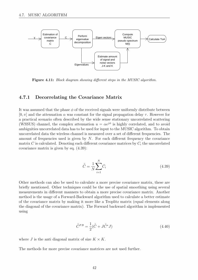
A block diagram showing the different steps in the MUSIC algorithm is found on fig. 4.11.
41
4.7. MUSIC ALGORITHM
Estimate amountof signal andnoise vectors
J-K and K
Eigenvalues
Eigen vectorsCyCalculate ToA
ComputeMUSIC
pseudo spectrumM(t)
Perform eigenvalue
decomposition
Estimation of covariance
matrixC
Figure 4.11: Block diagram showing different steps in the MUSIC algorithm.
4.7.1 Decorrelating the Covariance Matrix
It was assumed that the phase φ of the received signals were uniformly distribute between[0, π] and the attenuation α was constant for the signal propagation delay τ . However fora practical scenario often described by the wide sense stationary uncorrelated scattering(WSSUS) channel, the complex attenuation u = αejφ is highly correlated, and to avoidambiguities uncorrelated data has to be used for input to the MUSIC algorithm. To obtainuncorrelated data the wireless channel is measured over a set of different frequencies. Theamount of frequencies used is given by N . For each different frequency the covariancematrix C is calculated. Denoting each different covariance matrices by Ci the uncorrelatedcovariance matrix is given by eq. (4.39):
¯C =
1
N
N∑i=1
Ci (4.39)
Other methods can also be used to calculate a more precise covariance matrix, these arebriefly mentioned. Other techniques could be the use of spatial smoothing using severalmeasurements in different manners to obtain a more precise covariance matrix. Anothermethod is the usage of a Forward-Backward algorithm used to calculate a better estimateof the covariance matrix by making it more like a Teoplitz matrix (equal elements alongthe diagonal of the covariance matrix). The Forward backward algorithm is implementedusing
¯CFB =
1
2(
¯C + J
¯C∗J) (4.40)
where J is the anti diagonal matrix of size K ×K.
The methods for more precise covariance matrices are not used further.
42
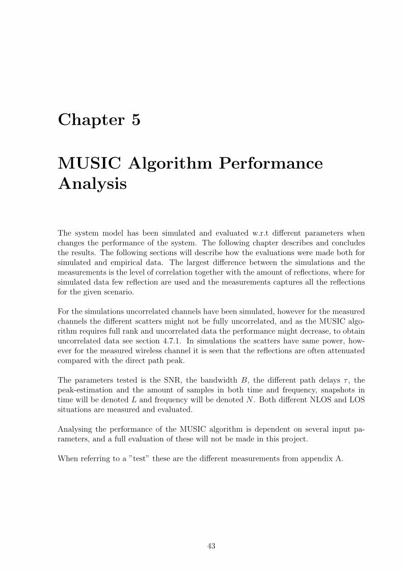
Chapter 5
MUSIC Algorithm PerformanceAnalysis
The system model has been simulated and evaluated w.r.t different parameters whenchanges the performance of the system. The following chapter describes and concludesthe results. The following sections will describe how the evaluations were made both forsimulated and empirical data. The largest difference between the simulations and themeasurements is the level of correlation together with the amount of reflections, where forsimulated data few reflection are used and the measurements captures all the reflectionsfor the given scenario.
For the simulations uncorrelated channels have been simulated, however for the measuredchannels the different scatters might not be fully uncorrelated, and as the MUSIC algo-rithm requires full rank and uncorrelated data the performance might decrease, to obtainuncorrelated data see section 4.7.1. In simulations the scatters have same power, how-ever for the measured wireless channel it is seen that the reflections are often attenuatedcompared with the direct path peak.
The parameters tested is the SNR, the bandwidth B, the different path delays τ , thepeak-estimation and the amount of samples in both time and frequency, snapshots intime will be denoted L and frequency will be denoted N . Both different NLOS and LOSsituations are measured and evaluated.
Analysing the performance of the MUSIC algorithm is dependent on several input pa-rameters, and a full evaluation of these will not be made in this project.
When referring to a ”test” these are the different measurements from appendix A.
43
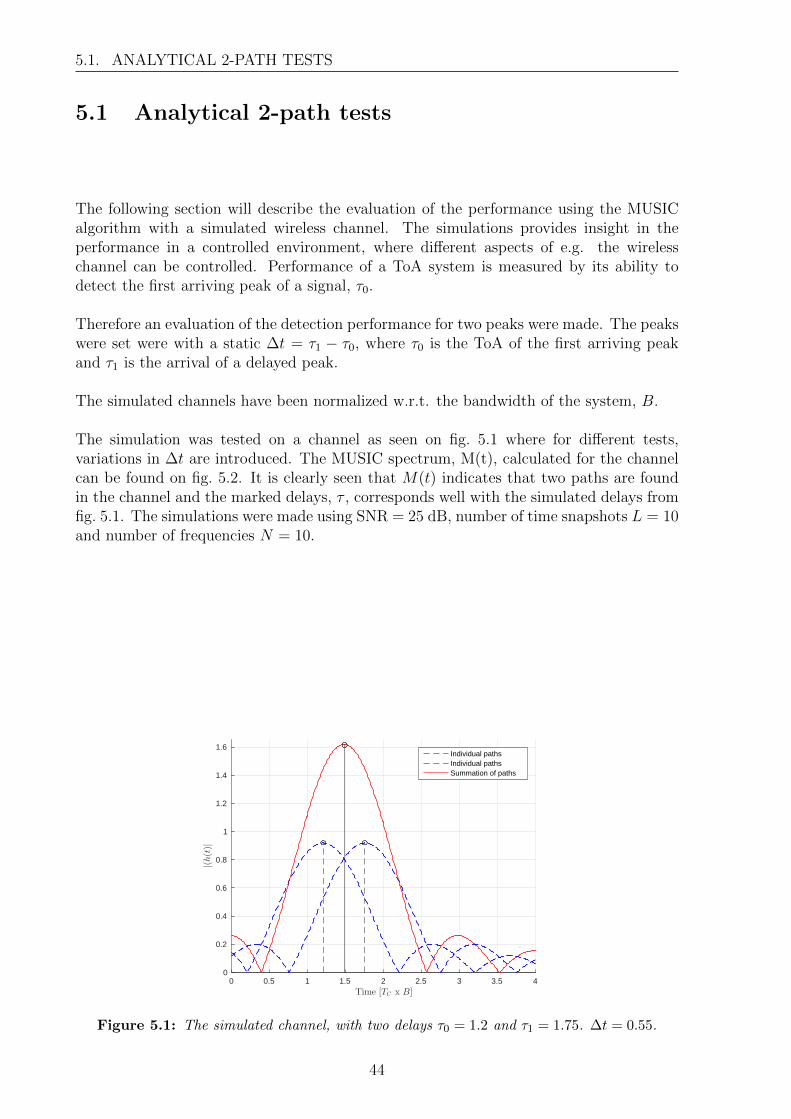
5.1. ANALYTICAL 2-PATH TESTS
5.1 Analytical 2-path tests
The following section will describe the evaluation of the performance using the MUSICalgorithm with a simulated wireless channel. The simulations provides insight in theperformance in a controlled environment, where different aspects of e.g. the wirelesschannel can be controlled. Performance of a ToA system is measured by its ability todetect the first arriving peak of a signal, τ0.
Therefore an evaluation of the detection performance for two peaks were made. The peakswere set were with a static ∆t = τ1 − τ0, where τ0 is the ToA of the first arriving peakand τ1 is the arrival of a delayed peak.
The simulated channels have been normalized w.r.t. the bandwidth of the system, B.
The simulation was tested on a channel as seen on fig. 5.1 where for different tests,variations in ∆t are introduced. The MUSIC spectrum, M(t), calculated for the channelcan be found on fig. 5.2. It is clearly seen that M(t) indicates that two paths are foundin the channel and the marked delays, τ , corresponds well with the simulated delays fromfig. 5.1. The simulations were made using SNR = 25 dB, number of time snapshots L = 10and number of frequencies N = 10.
0 0.5 1 1.5 2 2.5 3 3.5 4Time [TC x B]
0
0.2
0.4
0.6
0.8
1
1.2
1.4
1.6
|(h(t)|
Individual pathsIndividual pathsSummation of paths
Figure 5.1: The simulated channel, with two delays τ0 = 1.2 and τ1 = 1.75. ∆t = 0.55.
44
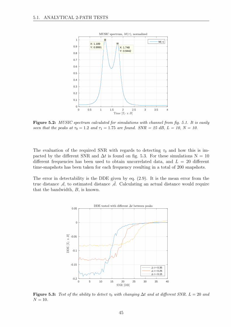
5.1. ANALYTICAL 2-PATH TESTS
0 0.5 1 1.5 2 2.5 3 3.5 4Time [TC x B]
0
0.1
0.2
0.3
0.4
0.5
0.6
0.7
0.8
0.9
1
MUSIC spectrum, M(τ), normalized
M( τ)
X: 1.748Y: 0.9442
X: 1.189Y: 0.9991
Figure 5.2: MUSIC spectrum calculated for simulations with channel from fig. 5.1. It is easilyseen that the peaks at τ0 = 1.2 and τ1 = 1.75 are found. SNR = 25 dB, L = 10, N = 10.
The evaluation of the required SNR with regards to detecting τ0 and how this is im-pacted by the different SNR and ∆t is found on fig. 5.3. For these simulations N = 10different frequencies has been used to obtain uncorrelated data, and L = 20 differenttime-snapshots has been taken for each frequency resulting in a total of 200 snapshots.
The error in detectability is the DDE given by eq. (2.9). It is the mean error from thetrue distance ,d, to estimated distance ,d. Calculating an actual distance would requirethat the bandwidth, B, is known.
0 5 10 15 20 25 30 35 40SNR [DB]
-0.2
-0.15
-0.1
-0.05
0
0.05
DDE[T
CxB]
DDE tested with different ∆t between peaks
∆ t = 0.35∆ t = 0.25∆ t = 0.15
Figure 5.3: Test of the ability to detect τ0 with changing ∆t and at different SNR. L = 20 andN = 10.
45
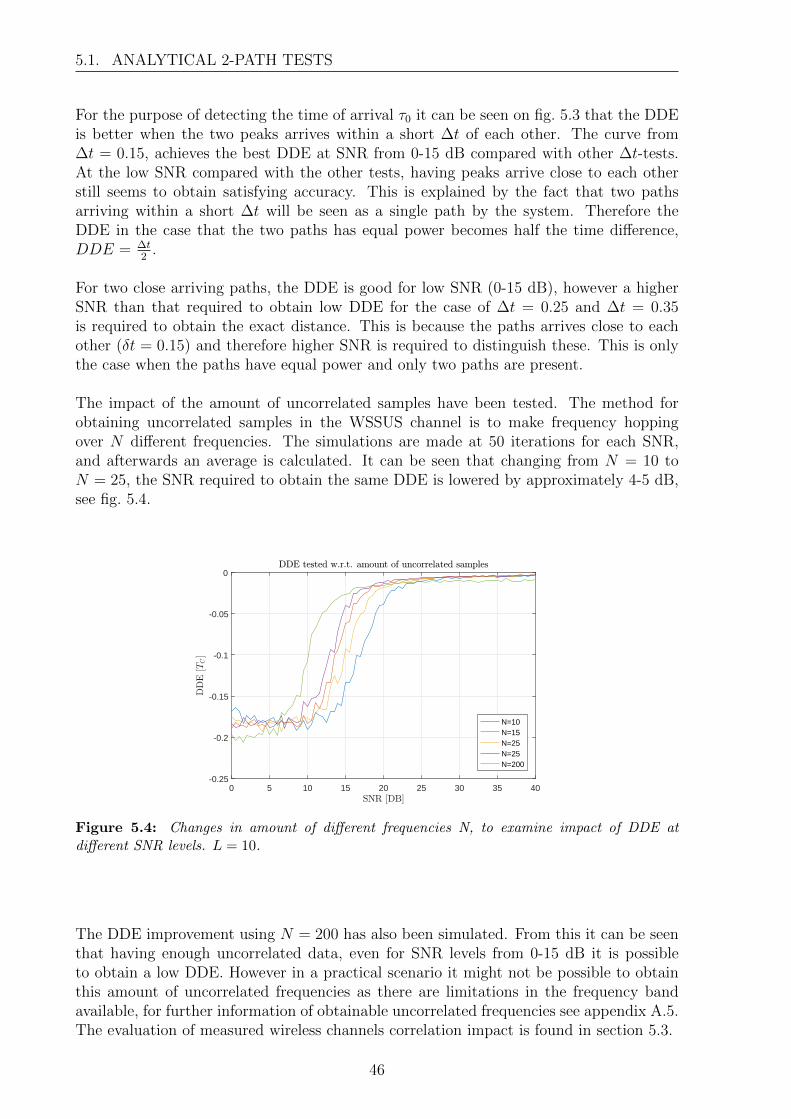
5.1. ANALYTICAL 2-PATH TESTS
For the purpose of detecting the time of arrival τ0 it can be seen on fig. 5.3 that the DDEis better when the two peaks arrives within a short ∆t of each other. The curve from∆t = 0.15, achieves the best DDE at SNR from 0-15 dB compared with other ∆t-tests.At the low SNR compared with the other tests, having peaks arrive close to each otherstill seems to obtain satisfying accuracy. This is explained by the fact that two pathsarriving within a short ∆t will be seen as a single path by the system. Therefore theDDE in the case that the two paths has equal power becomes half the time difference,DDE = ∆t
2.
For two close arriving paths, the DDE is good for low SNR (0-15 dB), however a higherSNR than that required to obtain low DDE for the case of ∆t = 0.25 and ∆t = 0.35is required to obtain the exact distance. This is because the paths arrives close to eachother (δt = 0.15) and therefore higher SNR is required to distinguish these. This is onlythe case when the paths have equal power and only two paths are present.
The impact of the amount of uncorrelated samples have been tested. The method forobtaining uncorrelated samples in the WSSUS channel is to make frequency hoppingover N different frequencies. The simulations are made at 50 iterations for each SNR,and afterwards an average is calculated. It can be seen that changing from N = 10 toN = 25, the SNR required to obtain the same DDE is lowered by approximately 4-5 dB,see fig. 5.4.
0 5 10 15 20 25 30 35 40-0.25
-0.2
-0.15
-0.1
-0.05
0
N=10N=15N=25N=25N=200
Figure 5.4: Changes in amount of different frequencies N, to examine impact of DDE atdifferent SNR levels. L = 10.
The DDE improvement using N = 200 has also been simulated. From this it can be seenthat having enough uncorrelated data, even for SNR levels from 0-15 dB it is possibleto obtain a low DDE. However in a practical scenario it might not be possible to obtainthis amount of uncorrelated frequencies as there are limitations in the frequency bandavailable, for further information of obtainable uncorrelated frequencies see appendix A.5.The evaluation of measured wireless channels correlation impact is found in section 5.3.
46
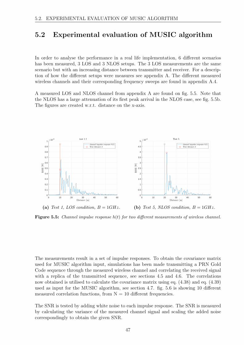
5.2. EXPERIMENTAL EVALUATION OF MUSIC ALGORITHM
5.2 Experimental evaluation of MUSIC algorithm
In order to analyse the performance in a real life implementation, 6 different scenarioshas been measured, 3 LOS and 3 NLOS setups. The 3 LOS measurements are the samescenario but with an increasing distance between transmitter and receiver. For a descrip-tion of how the different setups were measures see appendix A. The different measuredwireless channels and their corresponding frequency sweeps are found in appendix A.4.
A measured LOS and NLOS channel from appendix A are found on fig. 5.5. Note thatthe NLOS has a large attenuation of its first peak arrival in the NLOS case, see fig. 5.5b.The figures are created w.r.t. distance on the x-axis.
0 10 20 30 40 50 600
0.1
0.2
0.3
0.4
0.5
0.6
0.7
0.8
0.9
110-3
(a) Test 1, LOS condition, B = 1GHz.
0 10 20 30 40 50 600
0.5
1
1.5
2
2.5
3
3.5
4
4.5
510-4
(b) Test 5, NLOS condition, B = 1GHz.
Figure 5.5: Channel impulse response h(t) for two different measurements of wireless channel.
The measurements result in a set of impulse responses. To obtain the covariance matrixused for MUSIC algorithm input, simulations has been made transmitting a PRN GoldCode sequence through the measured wireless channel and correlating the received signalwith a replica of the transmitted sequence, see sections 4.5 and 4.6. The correlationsnow obtained is utilised to calculate the covariance matrix using eq. (4.38) and eq. (4.39)used as input for the MUSIC algorithm, see section 4.7. fig. 5.6 is showing 10 differentmeasured correlation functions, from N = 10 different frequencies.
The SNR is tested by adding white noise to each impulse response. The SNR is measuredby calculating the variance of the measured channel signal and scaling the added noisecorrespondingly to obtain the given SNR.
47
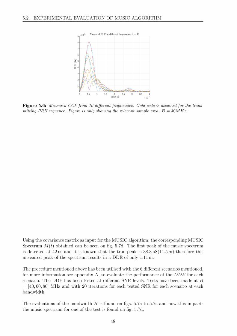
5.2. EXPERIMENTAL EVALUATION OF MUSIC ALGORITHM
0 0.5 1 1.5 2 2.5 3 3.5 4
10-7
1
2
3
4
5
6
7
8
910-5
Figure 5.6: Measured CCF from 10 different frequencies. Gold code is assumed for the trans-mitting PRN sequence. Figure is only showing the relevant sample area. B = 40MHz.
Using the covariance matrix as input for the MUSIC algorithm, the corresponding MUSICSpectrum M(t) obtained can be seen on fig. 5.7d. The first peak of the music spectrumis detected at 42 ns and it is known that the true peak is 38.3 nS(11.5 m) therefore thismeasured peak of the spectrum results in a DDE of only 1.11 m.
The procedure mentioned above has been utilised with the 6 different scenarios mentioned,for more information see appendix A, to evaluate the performance of the DDE for eachscenario. The DDE has been tested at different SNR levels. Tests have been made at B= [40, 60, 80] MHz and with 20 iterations for each tested SNR for each scenario at eachbandwidth.
The evaluations of the bandwidth B is found on figs. 5.7a to 5.7c and how this impactsthe music spectrum for one of the test is found on fig. 5.7d.
48
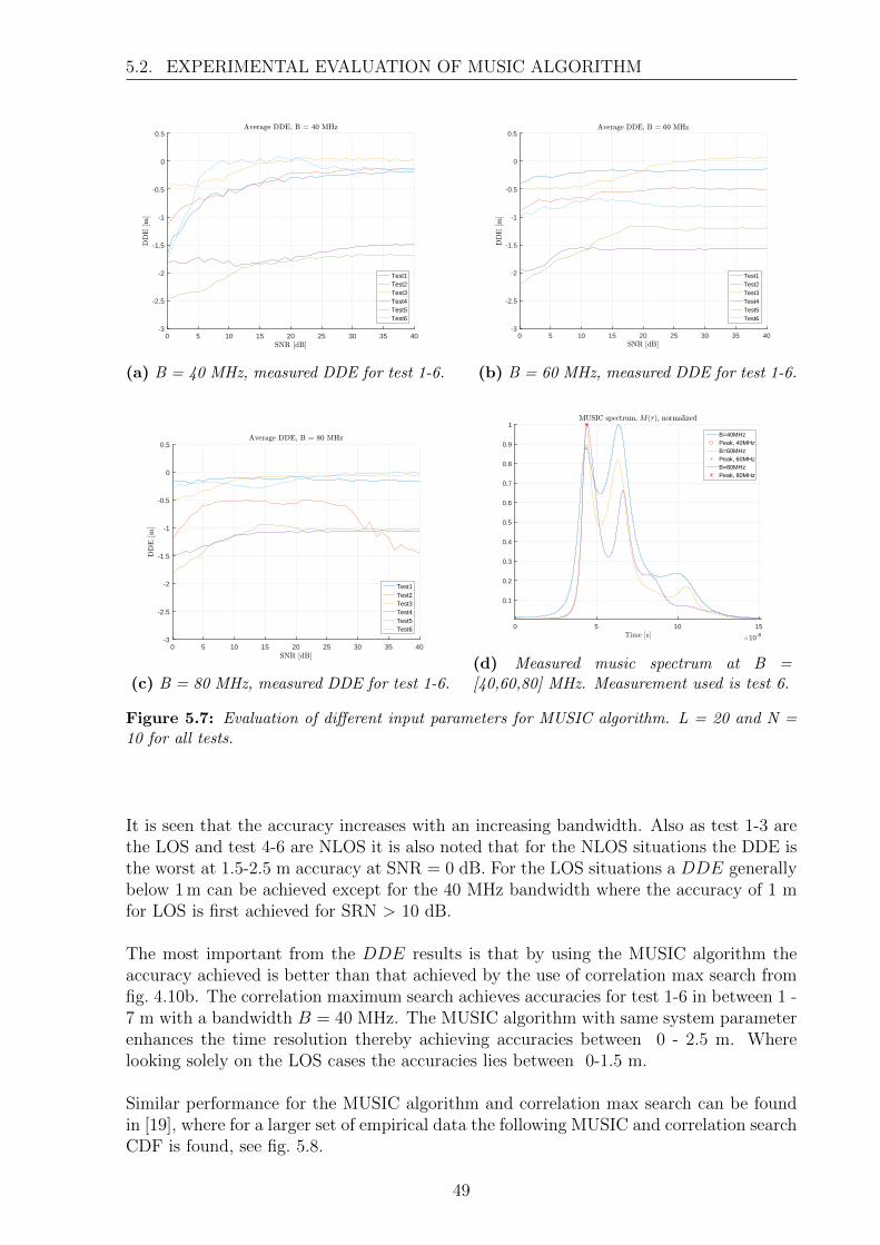
5.2. EXPERIMENTAL EVALUATION OF MUSIC ALGORITHM
0 5 10 15 20 25 30 35 40-3
-2.5
-2
-1.5
-1
-0.5
0
0.5
Test1Test2Test3Test4Test5Test6
(a) B = 40 MHz, measured DDE for test 1-6.
0 5 10 15 20 25 30 35 40-3
-2.5
-2
-1.5
-1
-0.5
0
0.5
Test1Test2Test3Test4Test5Test6
(b) B = 60 MHz, measured DDE for test 1-6.
0 5 10 15 20 25 30 35 40-3
-2.5
-2
-1.5
-1
-0.5
0
0.5
Test1Test2Test3Test4Test5Test6
(c) B = 80 MHz, measured DDE for test 1-6.
0 5 10 15
10-8
0.1
0.2
0.3
0.4
0.5
0.6
0.7
0.8
0.9
1B=40MHzPeak, 40MHzB=60MHzPeak, 60MHzB=80MHzPeak, 80MHz
(d) Measured music spectrum at B =[40,60,80] MHz. Measurement used is test 6.
Figure 5.7: Evaluation of different input parameters for MUSIC algorithm. L = 20 and N =10 for all tests.
It is seen that the accuracy increases with an increasing bandwidth. Also as test 1-3 arethe LOS and test 4-6 are NLOS it is also noted that for the NLOS situations the DDE isthe worst at 1.5-2.5 m accuracy at SNR = 0 dB. For the LOS situations a DDE generallybelow 1 m can be achieved except for the 40 MHz bandwidth where the accuracy of 1 mfor LOS is first achieved for SRN > 10 dB.
The most important from the DDE results is that by using the MUSIC algorithm theaccuracy achieved is better than that achieved by the use of correlation max search fromfig. 4.10b. The correlation maximum search achieves accuracies for test 1-6 in between 1 -7 m with a bandwidth B = 40 MHz. The MUSIC algorithm with same system parameterenhances the time resolution thereby achieving accuracies between 0 - 2.5 m. Wherelooking solely on the LOS cases the accuracies lies between 0-1.5 m.
Similar performance for the MUSIC algorithm and correlation max search can be foundin [19], where for a larger set of empirical data the following MUSIC and correlation searchCDF is found, see fig. 5.8.
49
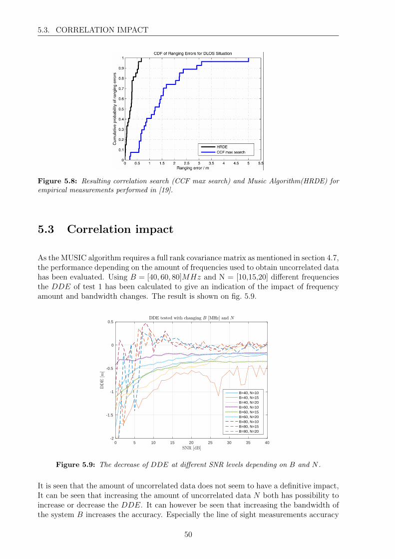
5.3. CORRELATION IMPACT
Figure 5.8: Resulting correlation search (CCF max search) and Music Algorithm(HRDE) forempirical measurements performed in [19].
5.3 Correlation impact
As the MUSIC algorithm requires a full rank covariance matrix as mentioned in section 4.7,the performance depending on the amount of frequencies used to obtain uncorrelated datahas been evaluated. Using B = [40, 60, 80]MHz and N = [10,15,20] different frequenciesthe DDE of test 1 has been calculated to give an indication of the impact of frequencyamount and bandwidth changes. The result is shown on fig. 5.9.
0 5 10 15 20 25 30 35 40SNR [dB]
-2
-1.5
-1
-0.5
0
0.5
DDE[m
]
DDE tested with changing B [MHz] and N
B=40, N=10B=40, N=15B=40, N=20B=60, N=10B=60, N=15B=60, N=20B=80, N=10B=80, N=15B=80, N=20
Figure 5.9: The decrease of DDE at different SNR levels depending on B and N .
It is seen that the amount of uncorrelated data does not seem to have a definitive impact,It can be seen that increasing the amount of uncorrelated data N both has possibility toincrease or decrease the DDE. It can however be seen that increasing the bandwidth ofthe system B increases the accuracy. Especially the line of sight measurements accuracy
50
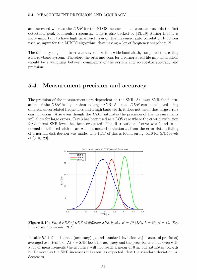
5.4. MEASUREMENT PRECISION AND ACCURACY
are increased whereas the DDE for the NLOS measurements saturates towards the firstdetectable peak of impulse responses. This is also backed by [13, 19] stating that it ismore important to have high time resolution on the measured auto correlation functionsused as input for the MUSIC algorithm, than having a lot of frequency snapshots N .
The difficulty might be to create a system with a wide bandwidth, compared to creatinga narrowband system. Therefore the pros and cons for creating a real life implementationshould be a weighting between complexity of the system and acceptable accuracy andprecision.
5.4 Measurement precision and accuracy
The precision of the measurements are dependent on the SNR. At lower SNR the fluctu-ations of the DDE is higher than at larger SNR. As small DDE can be achieved usingdifferent uncorrelated frequencies and a high bandwidth, it does not mean that large errorscan not occur. Also even though the DDE saturates the precision of the measurementsstill allow for large errors. Test 3 has been used as a LOS case where the error distributionfor different SNR levels has been evaluated. The distributions of error was found to benormal distributed with mean µ and standard deviation σ, from the error data a fittingof a normal distribution was made. The PDF of this is found on fig. 5.10 for SNR levelsof [0, 10, 20].
-1.2 -1 -0.8 -0.6 -0.4 -0.2 0 0.2 0.4DDE [m]
0
5
10
15
20
25
SNR
[dB]
Precision of measured DDE, normal distributed
SNR=0SNR=10SNR=20
Figure 5.10: Fitted PDF of DDE at different SNR-levels. B = 40 MHz, L = 20, N = 10. Test3 was used to generate PDF.
In table 5.1 is found a mean(accuracy), µ, and standard deviation, σ,(measure of precision)averaged over test 1-6. At low SNR both the accuracy and the precision are low, even witha lot of measurements the accuracy will not reach a mean of 0 m, but saturates towardsit. However as the SNR increases it is seen, as expected, that the standard deviation, σ,decreases.
51
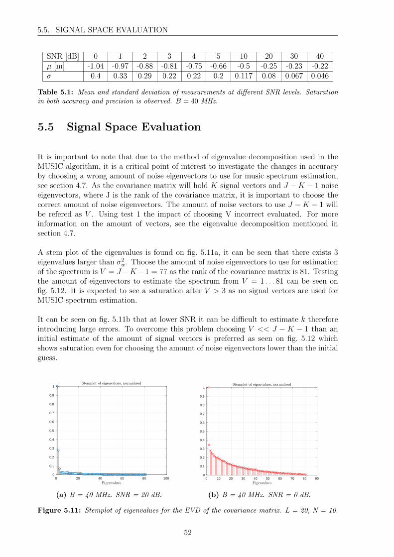
5.5. SIGNAL SPACE EVALUATION
SNR [dB] 0 1 2 3 4 5 10 20 30 40µ [m] -1.04 -0.97 -0.88 -0.81 -0.75 -0.66 -0.5 -0.25 -0.23 -0.22σ 0.4 0.33 0.29 0.22 0.22 0.2 0.117 0.08 0.067 0.046
Table 5.1: Mean and standard deviation of measurements at different SNR levels. Saturationin both accuracy and precision is observed. B = 40 MHz.
5.5 Signal Space Evaluation
It is important to note that due to the method of eigenvalue decomposition used in theMUSIC algorithm, it is a critical point of interest to investigate the changes in accuracyby choosing a wrong amount of noise eigenvectors to use for music spectrum estimation,see section 4.7. As the covariance matrix will hold K signal vectors and J −K − 1 noiseeigenvectors, where J is the rank of the covariance matrix, it is important to choose thecorrect amount of noise eigenvectors. The amount of noise vectors to use J −K − 1 willbe refered as V . Using test 1 the impact of choosing V incorrect evaluated. For moreinformation on the amount of vectors, see the eigenvalue decomposition mentioned insection 4.7.
A stem plot of the eigenvalues is found on fig. 5.11a, it can be seen that there exists 3eigenvalues larger than σ2
w. Thoose the amount of noise eigenvectors to use for estimationof the spectrum is V = J−K−1 = 77 as the rank of the covariance matrix is 81. Testingthe amount of eigenvectors to estimate the spectrum from V = 1 . . . 81 can be seen onfig. 5.12. It is expected to see a saturation after V > 3 as no signal vectors are used forMUSIC spectrum estimation.
It can be seen on fig. 5.11b that at lower SNR it can be difficult to estimate k thereforeintroducing large errors. To overcome this problem choosing V << J − K − 1 than aninitial estimate of the amount of signal vectors is preferred as seen on fig. 5.12 whichshows saturation even for choosing the amount of noise eigenvectors lower than the initialguess.
0 20 40 60 80 100Eigenvalues
0
0.1
0.2
0.3
0.4
0.5
0.6
0.7
0.8
0.9
1Stemplot of eigenvalues, normalized
(a) B = 40 MHz. SNR = 20 dB.
0 10 20 30 40 50 60 70 80 90Eigenvalues
0
0.1
0.2
0.3
0.4
0.5
0.6
0.7
0.8
0.9
1Stemplot of eigenvalues, normalized
(b) B = 40 MHz. SNR = 0 dB.
Figure 5.11: Stemplot of eigenvalues for the EVD of the covariance matrix. L = 20, N = 10.
52
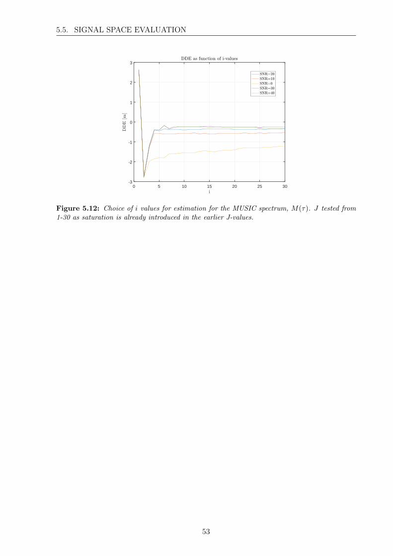
5.5. SIGNAL SPACE EVALUATION
0 5 10 15 20 25 30-3
-2
-1
0
1
2
3
Figure 5.12: Choice of i values for estimation for the MUSIC spectrum, M(τ). J tested from1-30 as saturation is already introduced in the earlier J-values.
53

Chapter 6
Conclusion
In this thesis the basic performance of indoor localisation systems was investigated. Chap-ter 3 consist of an analysis of different methods for indoor positioning, both the methodsused to calculate the positions of a tag, and the wireless channel characteristics whichcan be used to calculate input data for the positioning methods. Signal strength, Timeof Arrival and Angle of Arrival was investigated to evaluate the performance especiallyw.r.t. the changes in a wireless channel and the errors this introduces. The Time ofArrival system was concluded the most promising technique and the thesis transitionedinto an analysis of this.
For ToA as measure of distance different ToA detection methods was investigated. Thesebeing the general approach of using a correlation maximum search based on correlationproperties of the pseudo random noise codes used. And the use of the MUSIC algorithmto estimate the ToA based on a eigenvalue decomposition of the signal thereby exploitingthe properties of the signals to increase time resolution for better accuracy.
Further in chapter 4 a system description and model for a ToA system is described usedfor further simulation of the system and for describing what factors should be taken intoconsideration in a real life implementation. The evaluation of the correlation search isalso made and it is shown that accuracies for both LOS and NLOS in the area of 1 - 7 mcan be achieved using both simulated and empirical data. Lastly the section presents theMUSIC algorithm and describes the steps to obtain the MUSIC spectrum M(t).
Chapter 5 evaluates the MUSIC algorithm for simulations of the model described fora ToA system. For simulations the impact of scatter arrival, SNR and correlation wasevaluated. The measurements performed are examined and the MUSIC spectrum is usedto estimate the ToA of the first peak for the measured channels. Depending on theSNR, accuracies < 2.5m can be obtained for NLOS situations and errors < 1m can beachieved for LOS situations. It is also found that increasing the bandwidth B of thesystem increases performance of the accuracy. Going from B = 40MHz to B = 80MHzimproves the accuracy by 0.5-1 m. For SNR levels tested it is seen that the precisionincreases with increasing SNR, however for the empirical data the accuracy with enoughmeasurement does not seem to change. The amount of uncorrelated data was investigated
55
6.1. FUTURE WORK
and it is found that 10 sets of uncorrelated frequencies are sufficient for achieving goodaccuracy. It is seen from the NLOS cases that the estimation error has limitations forthis case as an undetected direct peak will not be present in the MUSIC spectrum.
The MUSIC algorithm is capable of enhancing the traditional method of correlation maxsearch. The higher time resolution provided for low bandwidth systems gives a significantimprovement in accuracy however it also increases the complexity of a system. ToA withhigher precision is possible to create using the MUSIC algorithm.
6.1 Future Work
As the MUSIC algorithm has been used and is a known signal processing technique,several varieties and improvement os this has been developed. For further improving thesystem and the corresponding DDE results implementations of these even more advanceMUSIC algorithms could be made. The MUSIC algorithms which is expected to improvethe systems performance is the EV (eigenvector) method. The reason for improvementsin this algorithm is that the noise eigenvectors are expecte to all be equal to σ2
w for atheoretical implementation. However for an actual estimate covariance matrix the noiseeigenvectors are 6= σ2
w and by utilising a normalisation with the eigenvalues it is foundin [14] that the MUSIC spectrum is less sensitive to inaccurate estimates of the noiseeigenvalues.
Therefore the music spectrum would be given by:
M(t) =1
J∑i=K+1
1λiβ∗i ·RP (τi)
(6.1)
where λ is the eigenvalue of the corresponding noise vector βi.
Also implementation of the Forward Backward algorithm mentioned in section 4.7 toobtain a toeplitz matrix could be implemented to further improve the estimation. AnotherMUSIC variant which is often used or referred to is the ROOT-MUSIC algorithm, thisalgorithm has however not been further investigated.
Other methods such as the ESPRIT algorithm is also widely used within the estimates ofAoA and ToA and should also be implemented and tested.
To evaluate the MUSIC algorithms performance, a more strategic approach to the mea-surement campaign should be made. This is a result of too few measurement having beenmade to evaluate the performance of the algorithm. Only 2 actual NLOS situations isseen from the measurements those being test 4 and 5 from appendix A. Especially longerdistances between transmitter and receiver should be measured and the performance in
56
6.1. FUTURE WORK
these situations should be evaluated against the performance of a corresponding correla-tion max search. It is also important to measure the wireless channels over time to see thefluctuations and estimate the SNR level whereas a more precise estimate of the impact ofnoise could be performed.
Further investigation woule also include a prototype for ToA measuring or several proto-types for setting up a TDoA system for testing and in- or decreasing accuracy using thissystem with the MUSIC algorithm.
For Further work should also be described the impact of the modulator and demodulator,together with a description of the errors these could introduce.
57

Bibliography
[1] “Indoor location market by component,” 2016.
[2] R. N. Zahid Farid and M. Ismail, “Recent advances in wireless indoor localiza-tion techniques and system,” Journal of Computer Networks and Communications,vol. 2013, pp. 1–12, 2013.
[3] H. Liu, H. Darabi, P. Banerjee, and J. Liu, “Survey of wireless indoor positioningtechniques and systems,” IEEE Transactions on Systems, Man, and Cybernetics,Part C (Applications and Reviews), vol. 37, pp. 1067–1080, Nov 2007.
[4] HP Invent, SmartLOCUS: An autonomous, self-assembling sensor network for indoorasset and systems management, June 2005.
[5] M. Werner, Indoor Location-Based Services. Springer, 2014. ISBN:978-3-319-10698-4.
[6] T. L. Beomju Shin, Jung Ho Lee and H. S. Kim, “Enhanced weighted k-nearestneighbor algorithm for indoor wi-fi positioning systems,” Computing Technology andInformation Management (ICCM), pp. 574–577, 2012.
[7] A. Ibrahim, S. K. A. Rahim, and H. Mohamad, “Performance evaluation of rss-based wsn indoor localization scheme using artificial neural network schemes,” in2015 IEEE 12th Malaysia International Conference on Communications (MICC),pp. 300–305, Nov 2015.
[8] L. S. Gus German, Quentin Spencer and R. Valenzuela, “Wireless indoor channelmodeling: Statistical agreement of ray tracing simulations and channel sounding mea-surements,” Acoustics, Speech, and Signal Processing, 1988, vol. 18, no. 4, pp. 2501–2504, 2001.
[9] M. A. J. Quentin H Spencer, Brian D Jeffs and A. L. Swindlehurst., “Modeling thestatistical time and angle of arrival characteristics of an indoor multipath channel,”IEEE JOURNAL ON SELECTED AREAS IN COMMUNICATIONS, vol. 18, no. 3,pp. 347–360, 2000.
[10] F. L. Y. Z. Jiuqiang Xu, Wei Liu and C. Wang, “Distance measurement model basedon rssi in wsn,” Wireless Sensor Network, vol. 2, no. 18, pp. 606–611, 2010.
59
BIBLIOGRAPHY
[11] Kegen Yu and Ian Sharp and Y. Jay Guo, Ground-Based Wireless Positioning. JohnWiley & sons Ltd.
[12] L. Jing, P. Liang, C. Maoyong, and S. Nongliang, “Super-resolution time of ar-rival estimation for indoor geolocation based on ieee 802.11 a/g,” in 2008 7th WorldCongress on Intelligent Control and Automation, pp. 6612–6615, June 2008.
[13] R. K. Michael Marx and H. C. Muller, “High resolution delay locked loop for timesynchronization with multi path mitigation,” Research in Microelectronics and Elec-tronics, pp. 204–207, 2009.
[14] X. Li, Performance of TOA Estimation Algorithms in Different Indoor MultipathConditions. Worcester Polytechnic Institute, 2003. Master Thesis.
[15] H. Farrokhi, “Toa estimation using music super-resolution techniques for an indooraudible chirp ranging system,” in 2007 IEEE International Conference on SignalProcessing and Communications, pp. 987–990, Nov 2007.
[16] “Quadrature iq.” Seen: 2017-02-22.
[17] “Gold code sequence,” 2008. Seen: 2017-02-15.
[18] R. Gold, “Optimal binary sequences for spread spectrum multiplexing (corresp.),”IEEE Transaction on Information Theory, vol. 13, no. 4, pp. 619–621, 1967.
[19] M. Marx, “System issues for time synchronization in real time localisation systemswith multi path mitigation,” 2010 European Wireless Conference, pp. 596–601, 2010.
[20] N. A. Alsindi, Super-Resolution TOA Estimation with Diversity Techniques for In-door Geolocation Application. Worcester Polytechnic Institute, 2004. Master Thesis.
60
Appendix A
Channel Measurement Description
A.1 Purpose of Measurements
To evaluate the MUSIC algorithm in a real life implementation it is important to havemeasurements for a different set of scenarios and distances. Simulations does not repre-sent the wireless characteristics to same degree as actual measurements which capturesboth attenuations and multipath effects. The following appendix will describe how thedifferent measurements were conducted, and how the post-processing of frequency- andtime-domain data were made.
A.2 Setup
For measuring the wireless channel a network analyser, namely the Agilent N5227A versionA.09.80.20, was used.
A frequency sweep were measured from f = 2 GHz – 3 GHz with a frequency stepping of∆f = 500 KHz.
For transmitting and receiving antenna were used two Suhner SWA 0859/360/4/10/Vplanar antennas. The antenna pattern at the frequency range does not change much,therefore patterns only for 2.3 GHz and 2.7 GHz is shown, see figs. A.1a and A.1b.
61
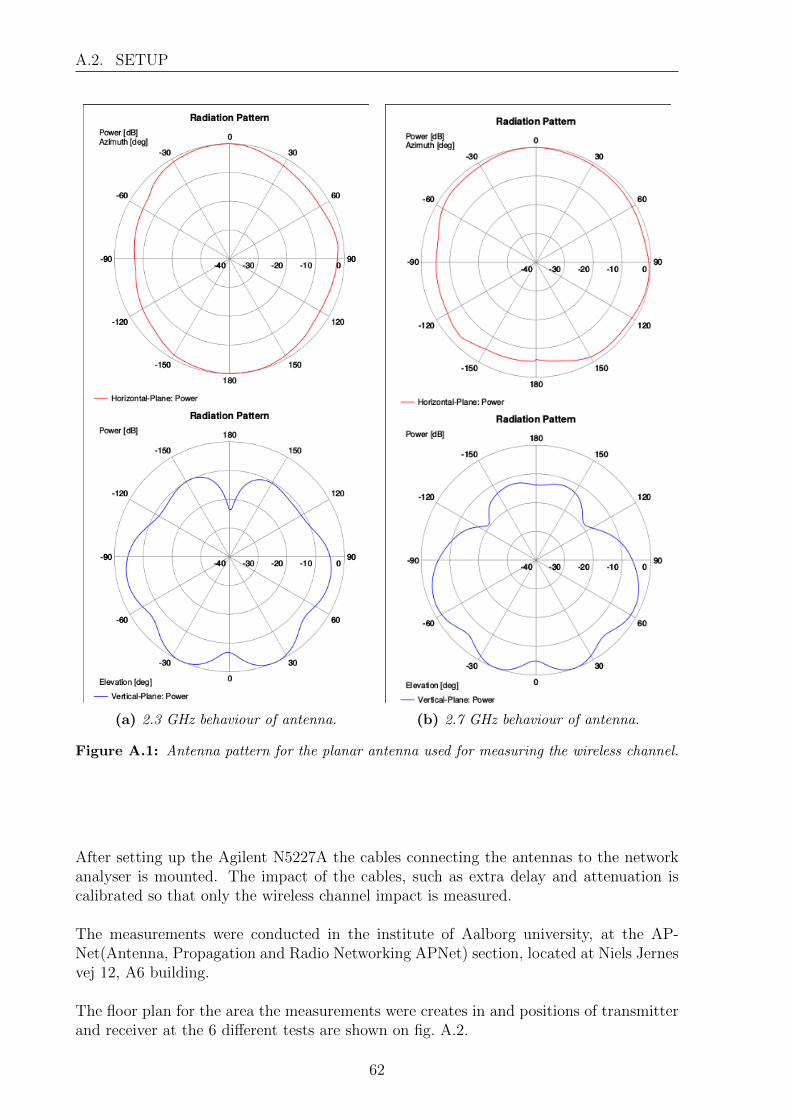
A.2. SETUP
(a) 2.3 GHz behaviour of antenna. (b) 2.7 GHz behaviour of antenna.
Figure A.1: Antenna pattern for the planar antenna used for measuring the wireless channel.
After setting up the Agilent N5227A the cables connecting the antennas to the networkanalyser is mounted. The impact of the cables, such as extra delay and attenuation iscalibrated so that only the wireless channel impact is measured.
The measurements were conducted in the institute of Aalborg university, at the AP-Net(Antenna, Propagation and Radio Networking APNet) section, located at Niels Jernesvej 12, A6 building.
The floor plan for the area the measurements were creates in and positions of transmitterand receiver at the 6 different tests are shown on fig. A.2.
62
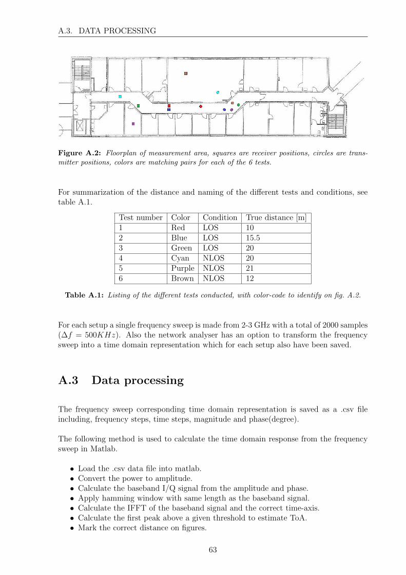
A.3. DATA PROCESSING
Figure A.2: Floorplan of measurement area, squares are receiver positions, circles are trans-mitter positions, colors are matching pairs for each of the 6 tests.
For summarization of the distance and naming of the different tests and conditions, seetable A.1.
Test number Color Condition True distance [m]1 Red LOS 102 Blue LOS 15.53 Green LOS 204 Cyan NLOS 205 Purple NLOS 216 Brown NLOS 12
Table A.1: Listing of the different tests conducted, with color-code to identify on fig. A.2.
For each setup a single frequency sweep is made from 2-3 GHz with a total of 2000 samples(∆f = 500KHz). Also the network analyser has an option to transform the frequencysweep into a time domain representation which for each setup also have been saved.
A.3 Data processing
The frequency sweep corresponding time domain representation is saved as a .csv fileincluding, frequency steps, time steps, magnitude and phase(degree).
The following method is used to calculate the time domain response from the frequencysweep in Matlab.
• Load the .csv data file into matlab.• Convert the power to amplitude.• Calculate the baseband I/Q signal from the amplitude and phase.• Apply hamming window with same length as the baseband signal.• Calculate the IFFT of the baseband signal and the correct time-axis.• Calculate the first peak above a given threshold to estimate ToA.• Mark the correct distance on figures.
63
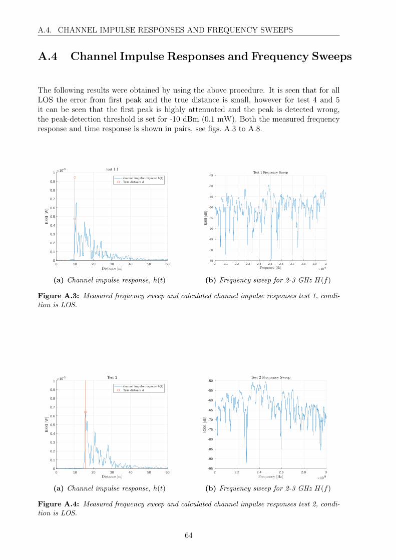
A.4. CHANNEL IMPULSE RESPONSES AND FREQUENCY SWEEPS
A.4 Channel Impulse Responses and Frequency Sweeps
The following results were obtained by using the above procedure. It is seen that for allLOS the error from first peak and the true distance is small, however for test 4 and 5it can be seen that the first peak is highly attenuated and the peak is detected wrong,the peak-detection threshold is set for -10 dBm (0.1 mW). Both the measured frequencyresponse and time response is shown in pairs, see figs. A.3 to A.8.
0 10 20 30 40 50 600
0.1
0.2
0.3
0.4
0.5
0.6
0.7
0.8
0.9
110-3
(a) Channel impulse response, h(t)
2 2.1 2.2 2.3 2.4 2.5 2.6 2.7 2.8 2.9 3Frequency [Hz]
×10 9
-85
-80
-75
-70
-65
-60
-55
-50
-45
RSSI[dB]
Test 1 Frequency Sweep
(b) Frequency sweep for 2-3 GHz H(f)
Figure A.3: Measured frequency sweep and calculated channel impulse responses test 1, condi-tion is LOS.
0 10 20 30 40 50 600
0.1
0.2
0.3
0.4
0.5
0.6
0.7
0.8
0.9
110-3
(a) Channel impulse response, h(t)
2 2.2 2.4 2.6 2.8 3Frequency [Hz]
×10 9
-95
-90
-85
-80
-75
-70
-65
-60
-55
-50
RSSI[dB]
Test 2 Frequency Sweep
(b) Frequency sweep for 2-3 GHz H(f)
Figure A.4: Measured frequency sweep and calculated channel impulse responses test 2, condi-tion is LOS.
64
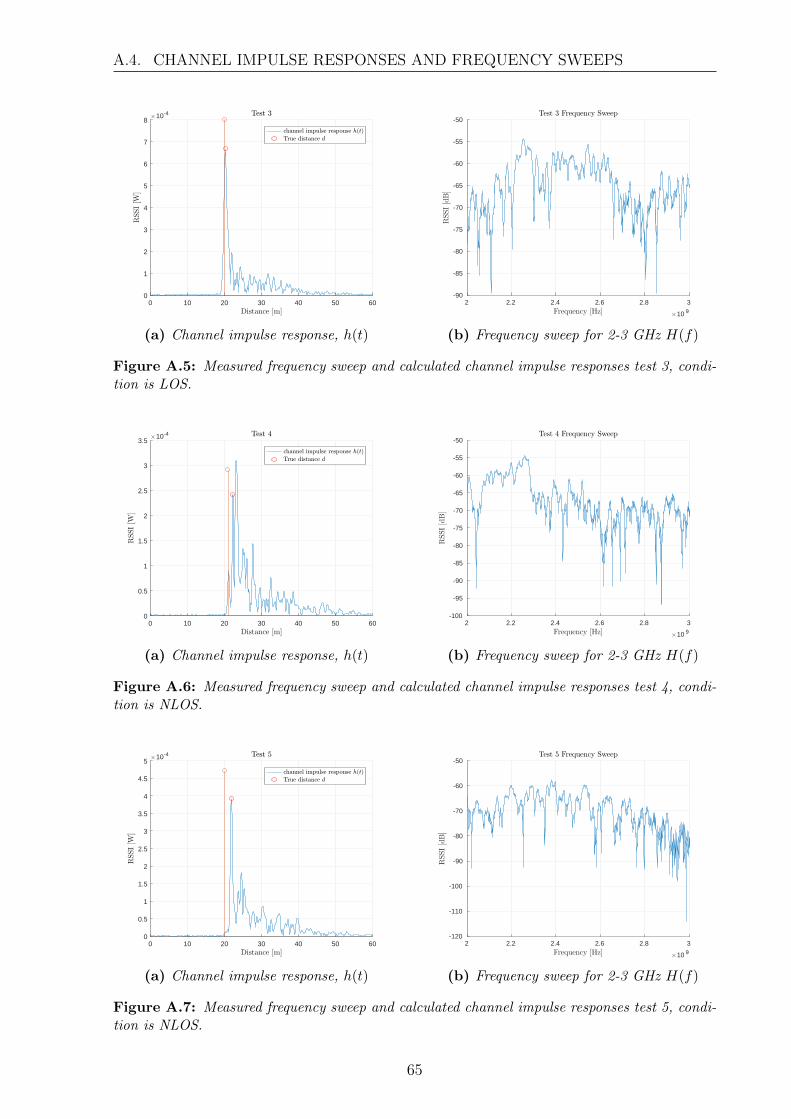
A.4. CHANNEL IMPULSE RESPONSES AND FREQUENCY SWEEPS
0 10 20 30 40 50 600
1
2
3
4
5
6
7
810-4
(a) Channel impulse response, h(t)
2 2.2 2.4 2.6 2.8 3Frequency [Hz]
×10 9
-90
-85
-80
-75
-70
-65
-60
-55
-50
RSSI[dB]
Test 3 Frequency Sweep
(b) Frequency sweep for 2-3 GHz H(f)
Figure A.5: Measured frequency sweep and calculated channel impulse responses test 3, condi-tion is LOS.
0 10 20 30 40 50 600
0.5
1
1.5
2
2.5
3
3.510-4
(a) Channel impulse response, h(t)
2 2.2 2.4 2.6 2.8 3Frequency [Hz]
×10 9
-100
-95
-90
-85
-80
-75
-70
-65
-60
-55
-50RSSI[dB]
Test 4 Frequency Sweep
(b) Frequency sweep for 2-3 GHz H(f)
Figure A.6: Measured frequency sweep and calculated channel impulse responses test 4, condi-tion is NLOS.
0 10 20 30 40 50 600
0.5
1
1.5
2
2.5
3
3.5
4
4.5
510-4
(a) Channel impulse response, h(t)
2 2.2 2.4 2.6 2.8 3Frequency [Hz]
×10 9
-120
-110
-100
-90
-80
-70
-60
-50
RSSI[dB]
Test 5 Frequency Sweep
(b) Frequency sweep for 2-3 GHz H(f)
Figure A.7: Measured frequency sweep and calculated channel impulse responses test 5, condi-tion is NLOS.
65
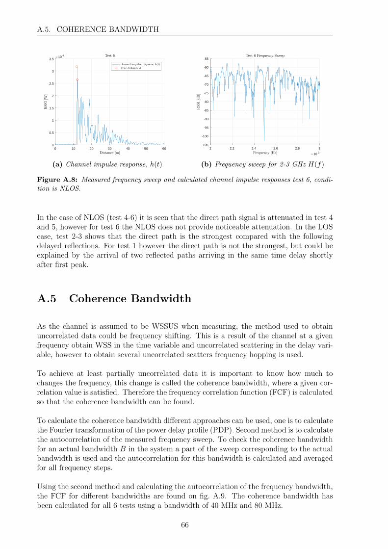
A.5. COHERENCE BANDWIDTH
0 10 20 30 40 50 600
0.5
1
1.5
2
2.5
3
3.510-4
(a) Channel impulse response, h(t)
2 2.2 2.4 2.6 2.8 3Frequency [Hz]
×10 9
-105
-100
-95
-90
-85
-80
-75
-70
-65
-60
-55
RSSI[dB]
Test 6 Frequency Sweep
(b) Frequency sweep for 2-3 GHz H(f)
Figure A.8: Measured frequency sweep and calculated channel impulse responses test 6, condi-tion is NLOS.
In the case of NLOS (test 4-6) it is seen that the direct path signal is attenuated in test 4and 5, however for test 6 the NLOS does not provide noticeable attenuation. In the LOScase, test 2-3 shows that the direct path is the strongest compared with the followingdelayed reflections. For test 1 however the direct path is not the strongest, but could beexplained by the arrival of two reflected paths arriving in the same time delay shortlyafter first peak.
A.5 Coherence Bandwidth
As the channel is assumed to be WSSUS when measuring, the method used to obtainuncorrelated data could be frequency shifting. This is a result of the channel at a givenfrequency obtain WSS in the time variable and uncorrelated scattering in the delay vari-able, however to obtain several uncorrelated scatters frequency hopping is used.
To achieve at least partially uncorrelated data it is important to know how much tochanges the frequency, this change is called the coherence bandwidth, where a given cor-relation value is satisfied. Therefore the frequency correlation function (FCF) is calculatedso that the coherence bandwidth can be found.
To calculate the coherence bandwidth different approaches can be used, one is to calculatethe Fourier transformation of the power delay profile (PDP). Second method is to calculatethe autocorrelation of the measured frequency sweep. To check the coherence bandwidthfor an actual bandwidth B in the system a part of the sweep corresponding to the actualbandwidth is used and the autocorrelation for this bandwidth is calculated and averagedfor all frequency steps.
Using the second method and calculating the autocorrelation of the frequency bandwidth,the FCF for different bandwidths are found on fig. A.9. The coherence bandwidth hasbeen calculated for all 6 tests using a bandwidth of 40 MHz and 80 MHz.
66
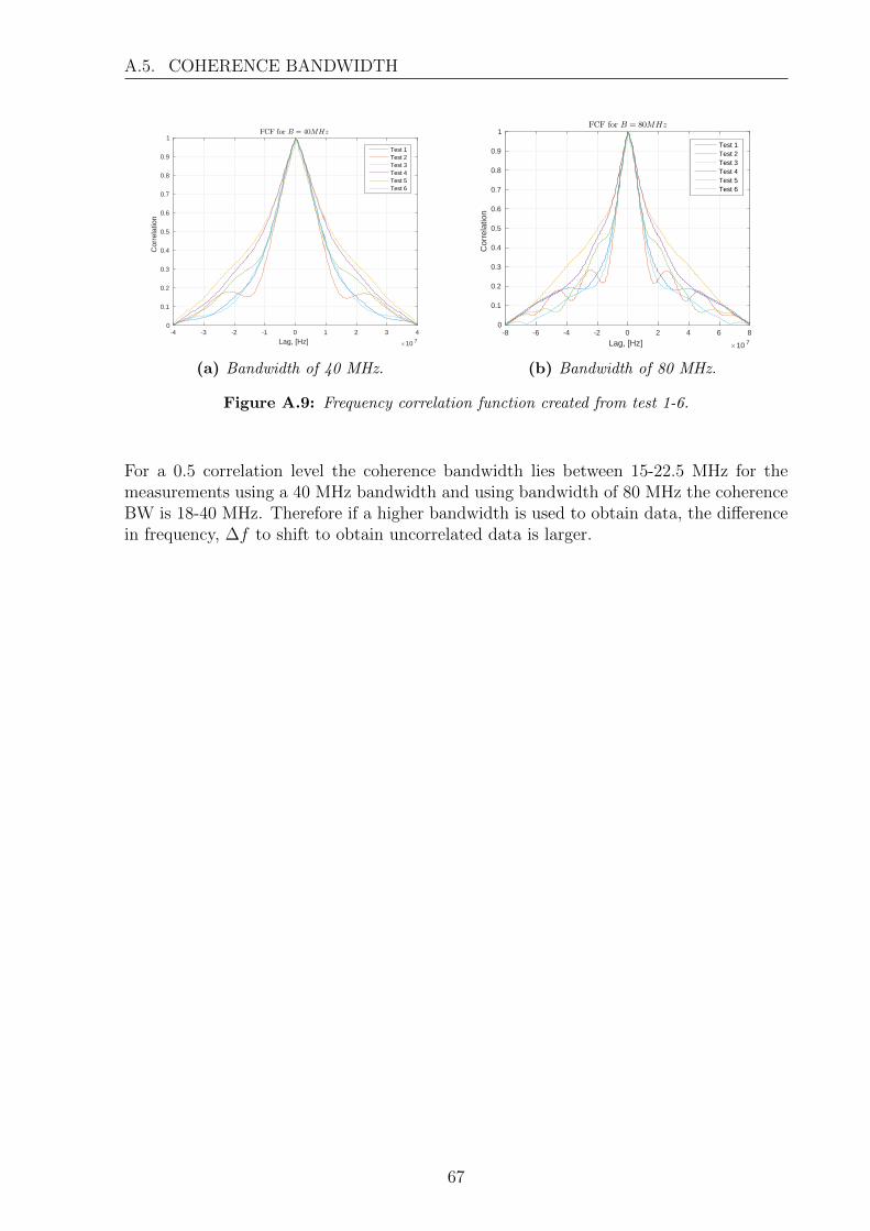
A.5. COHERENCE BANDWIDTH
-4 -3 -2 -1 0 1 2 3 4
Lag, [Hz]×10 7
0
0.1
0.2
0.3
0.4
0.5
0.6
0.7
0.8
0.9
1
Cor
rela
tion
FCF for B = 40MHz
Test 1Test 2Test 3Test 4Test 5Test 6
(a) Bandwidth of 40 MHz.
-8 -6 -4 -2 0 2 4 6 8
Lag, [Hz]×10 7
0
0.1
0.2
0.3
0.4
0.5
0.6
0.7
0.8
0.9
1
Cor
rela
tion
FCF for B = 80MHz
Test 1Test 2Test 3Test 4Test 5Test 6
(b) Bandwidth of 80 MHz.
Figure A.9: Frequency correlation function created from test 1-6.
For a 0.5 correlation level the coherence bandwidth lies between 15-22.5 MHz for themeasurements using a 40 MHz bandwidth and using bandwidth of 80 MHz the coherenceBW is 18-40 MHz. Therefore if a higher bandwidth is used to obtain data, the differencein frequency, ∆f to shift to obtain uncorrelated data is larger.
67

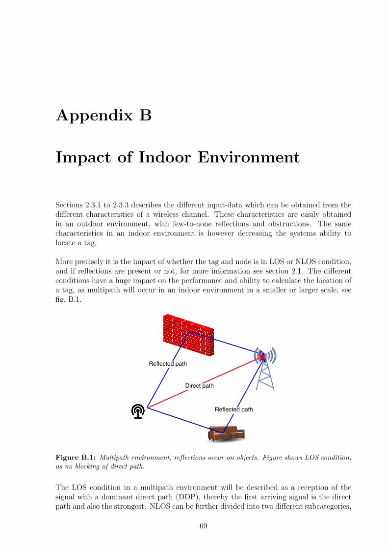
Appendix B
Impact of Indoor Environment
Sections 2.3.1 to 2.3.3 describes the different input-data which can be obtained from thedifferent characteristics of a wireless channel. These characteristics are easily obtainedin an outdoor environment, with few-to-none reflections and obstructions. The samecharacteristics in an indoor environment is however decreasing the systems ability tolocate a tag.
More precisely it is the impact of whether the tag and node is in LOS or NLOS condition,and if reflections are present or not, for more information see section 2.1. The differentconditions have a huge impact on the performance and ability to calculate the location ofa tag, as multipath will occur in an indoor environment in a smaller or larger scale, seefig. B.1.
Figure B.1: Multipath environment, reflections occur on objects. Figure shows LOS condition,as no blocking of direct path.
The LOS condition in a multipath environment will be described as a reception of thesignal with a dominant direct path (DDP), thereby the first arriving signal is the directpath and also the strongest. NLOS can be further divided into two different subcategories,
69
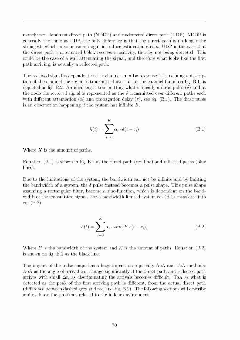
namely non dominant direct path (NDDP) and undetected direct path (UDP). NDDP isgenerally the same as DDP, the only difference is that the direct path is no longer thestrongest, which in some cases might introduce estimation errors. UDP is the case thatthe direct path is attenuated below receiver sensitivity, thereby not being detected. Thiscould be the case of a wall attenuating the signal, and therefore what looks like the firstpath arriving, is actually a reflected path.
The received signal is dependent on the channel impulse response (h), meaning a descrip-tion of the channel the signal is transmitted over. h for the channel found on fig. B.1, isdepicted as fig. B.2. An ideal tag is transmitting what is ideally a dirac pulse (δ) and atthe node the received signal is represented as the δ transmitted over different paths eachwith different attenuation (α) and propagation delay (τ), see eq. (B.1). The dirac pulseis an observation happening if the system has infinite B.
h(t) =
K∑i=0
αi · δ(t− τi) (B.1)
Where K is the amount of paths.
Equation (B.1) is shown in fig. B.2 as the direct path (red line) and reflected paths (bluelines).
Due to the limitations of the system, the bandwidth can not be infinite and by limitingthe bandwidth of a system, the δ pulse instead becomes a pulse shape. This pulse shapeassuming a rectangular filter, become a sinc-function, which is dependent on the band-width of the transmitted signal. For a bandwidth limited system eq. (B.1) translates intoeq. (B.2).
h(t) =
K∑i=0
αi · sinc(B · (t− τi)) (B.2)
Where B is the bandwidth of the system and K is the amount of paths. Equation (B.2)is shown on fig. B.2 as the black line.
The impact of the pulse shape has a huge impact on especially AoA and ToA methods.AoA as the angle of arrival can change significantly if the direct path and reflected patharrives with small ∆t, as discriminating the arrivals becomes difficult. ToA as what isdetected as the peak of the first arriving path is different, from the actual direct path(difference between dashed grey and red line, fig. B.2). The following sections will describeand evaluate the problems related to the indoor environment.
70
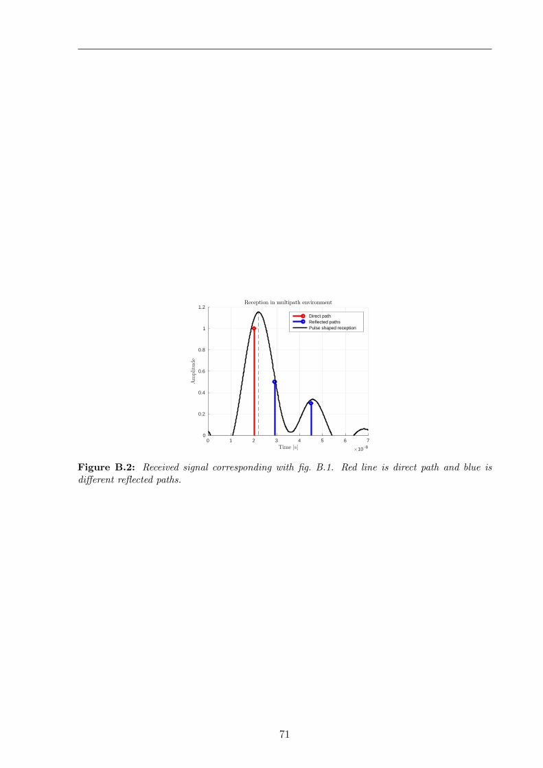
0 1 2 3 4 5 6 7Time [s]
×10 -8
0
0.2
0.4
0.6
0.8
1
1.2
Amplitude
Reception in multipath environment
Direct pathReflected pathsPulse shaped reception
Figure B.2: Received signal corresponding with fig. B.1. Red line is direct path and blue isdifferent reflected paths.
71