These notes can serve as a mathematical supplamnt to the standard graduate

level texts on general re la t ivi ty and are suitable for selfstudy. The exposition

is detailed and includes accounts of several topics of current interest, e.g.,

Lovelock theory and Ashtekar's variables.

MATHEMATICAL ASPECTS OF GENERAL R E L A T I V I T Y

Garth Warner

Department of Mathematics

University of Washington

CONTENTS

Introduction

Geometric Quantities

Scalar Products

Interior Multiplication

Tensor Analysis

Lie Derivatives

Flows

Covariant Differentiation

Parallel Transport

Curvature

Semiriemannian Manifolds

The Einstein Equation

Decomposition Theory

Bundle Valued Forms

The Structural Equations

Transition Generalities

Metric Considerations

Submanifolds

Extrinsic Curvature

Hodge Conventions

Star Formulae

Metric Concomitants

Lagrangians

The Euler-Lagrange Equations

The Helmholtz Condition

Applications of Homogeneity

Questions of Uniqueness

Globalization

Functional Derivatives

Variational Principles

Splittings

Metrics on Metrics

The Symplectic Structure

Motion in a Potential

Constant Lapse, Zero Shift

Variable Lapse, Zero Shift

Incorporation of the Shift

Dynamics

Causality

The Standard Setup

Isolating the Lagrangian

The Momentum Form

Elimination of the Metric

Constraints in the Coframe Picture

Evolution in the Coframe Picture

Computation of the Poisson Brackets

Field Equations

Lovelock Gravity

The Palatini Formalism

Torsion

Extending the Theory

Evolution in the Palatini Picture

Expansion of the Phase Space

Extension of the Scalars

Selfdual Algebra

The Selfdual Lagrangian

Two Canonical Transformations

Ashtekar's Hamiltonian

Evolution in the Ashtekar Picture

The Constraint Analysis

Densitized Variables

Rescaling the Theory

Asymptotic Flatness

The Integrals of Motion-Energy and Center of Mass

The Integrals of Motion-Linear and Angular Momentum

Modifying the Hamiltonian

The ~oincarg Structure

Function Spaces

Asymptotically Euclidean Riemannian Structures

Laplacians

Positive Energy

References:

- Books

- Articles

Section 0: Introduction A preliminary version of these notes was

distributed to the participants in a seminar on quantum gravity which I gave

a couple of years ago. As they seered to be rather well received, I decided

that a revised and expanded account might be useful for a wider audience.

Like the original, the focus is on the formalism underlying general

relativity, thus there is no physics and virtually no discussion of exact

solutions. Wre seriously, the Cauchy problem is not considered. My only

defense for such an cmission is that certain cbices have to be made and to

do the matter justice muld require another b k .

The prerequisites are modest: Just sane differential g-try, much of

which is reviewed in the text anyway. As for what is covered, scsrne of the topics

are standard, others less so. Included anlong the latter is a proof of the

mvelock uniqueness theorem, a systematic discussion of the Palatini formlism,

a cclmplete global treatmnt of the Ashtekar variables, and an introduction to

the asymptotic theory.

For the mst part, the exposition is detail oriented and directed toward

the beginner, not the expert. Frankly, I tire quickly of phrases like: "it

follows readily" or "one sbws without difficulty" or "a short calculation gives"

or "it is easy to see that" EXC. To be sure I have left sane things for the

reader to mrk out but I have tried not to make a habit of it.

While I have yet to get around to compiling an index, the text is not too

difficult to navigate given the number of section headings.

Naturally, I muld like to hear about any typos or outright errors and

ccarments and suggestions for improvement muld be much appreciated.

Section 1: Cmetric Quantities Let V be an n-dimmional real vector

space and let V* be its dual.

Notation: B(V) is the set of ordered bases for V.

The general linear group - GL(n,R) - oprates to the r ight on B (V) :

[Note: Therefore raw vector conventions are in force: E-g is cmputed

by inspection of

If B (V*) stands for the set of ordered bases i n V*, Lhen GL - (n,R) - operates

-1 T to the r ight on B (V*) via duality, i . e . , via multiplication by (g ) . Given a basis E = {E1,...,E } € B(V) , its cobasis o = {wl,...,wn} E B(V*)

n

is defined by wi (F 1 = 6 i

' j j '

Observation: Let g E - GL(n,s) -- then the cobasis corresponding to E-g is

w-g.

[Since

it follows that

[Note: From the definitions,

which explains the flip in the i1dices.1

T E V ~ is a multilinear map q

hence admits an expansion

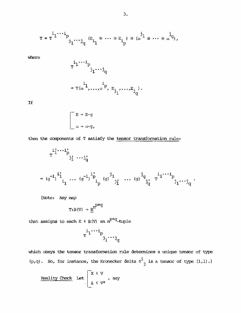
w h e r e

then the components of T satisfy the tensor transformation rule:

[ N o t e : Any map

that assigns to each E E B (V) an n*-tuple

which obeys the tensor transformation rule determines a unique tensor of type

(p, q) . So, for instance, the Kronecker delta is a tensor of type (1,l) .I j

Reality Check Let I say n c v *

(A. = A ( E . ) ) . 3 3

i N m change the basis: E -+ E * g -- then X = X ( E * g ) i l , where

IEMW There is a canonical i m r p h i s n

and extend by linearity. 1

[Note: Take pl=O, q' =O to conclude that vq is the dual of vP. 1 P 4

Products There is a map

viz .

In terms of cmponents,

il.. .iwpl (T €4 T')

jl- .jq*'

In t e r m s of camponents,

Definition: The Kronecker symbol of order p is the tensor of type (p,p)

defined by

Then

vanishes i f IfJ but is

1-+1 i f I is an even permutation of J

I -1 i f I is an cdd permutation of J. -

[Note: The Kronecker symbol of order p is antisymnetric under interchange

of any .two of the indices il, ..., i or under interchange of any two of the P

indices jl,..., . j P

coincide, then

which is autcaMtic

Example: Let

Put

So, if any t m of the indices il,...,i or j ,..., P 1 j p

Then

belongs to A%.

Note: If T E A'V to begin with, then Alt T = T, hence Alto ALt = Alt.

As an element of VO the ccanponents of Alt T are given by P '

FACT Suppose that q<p -- then

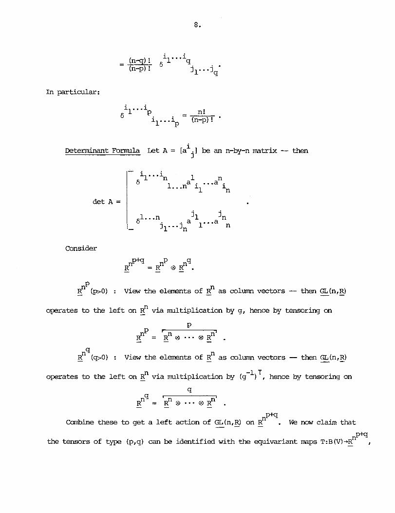
In particular:

i l.. .ip 6 - - n!

i, ... i (n-p)! ' P

Deterrmnan i

t Fomrula Let A = [a . I be an n-by-n matrix -- then 3

det

Consider

P n Rn (PO) : View the e ~ ~ t ~ of R as column vectors -- then GL (n, R) - - - -

operates to the left on - Rn via multiplication by g, hence by tensoring on

P

q Rn ( ~ 0 ) : View the elements of Rn as column vectors -- then GL(n,E) - - -

-1 T operates to the left on - Rn via multiplication by (g ) , hence by tensoring on

q I

Rn = Rn @ --• @, I("' . - - F"¶

Ccanbine these to get a left action of GL (n,~) on Rn . We - - -

the tensors of type (p,q) can be identified with the equivariant

now claim that

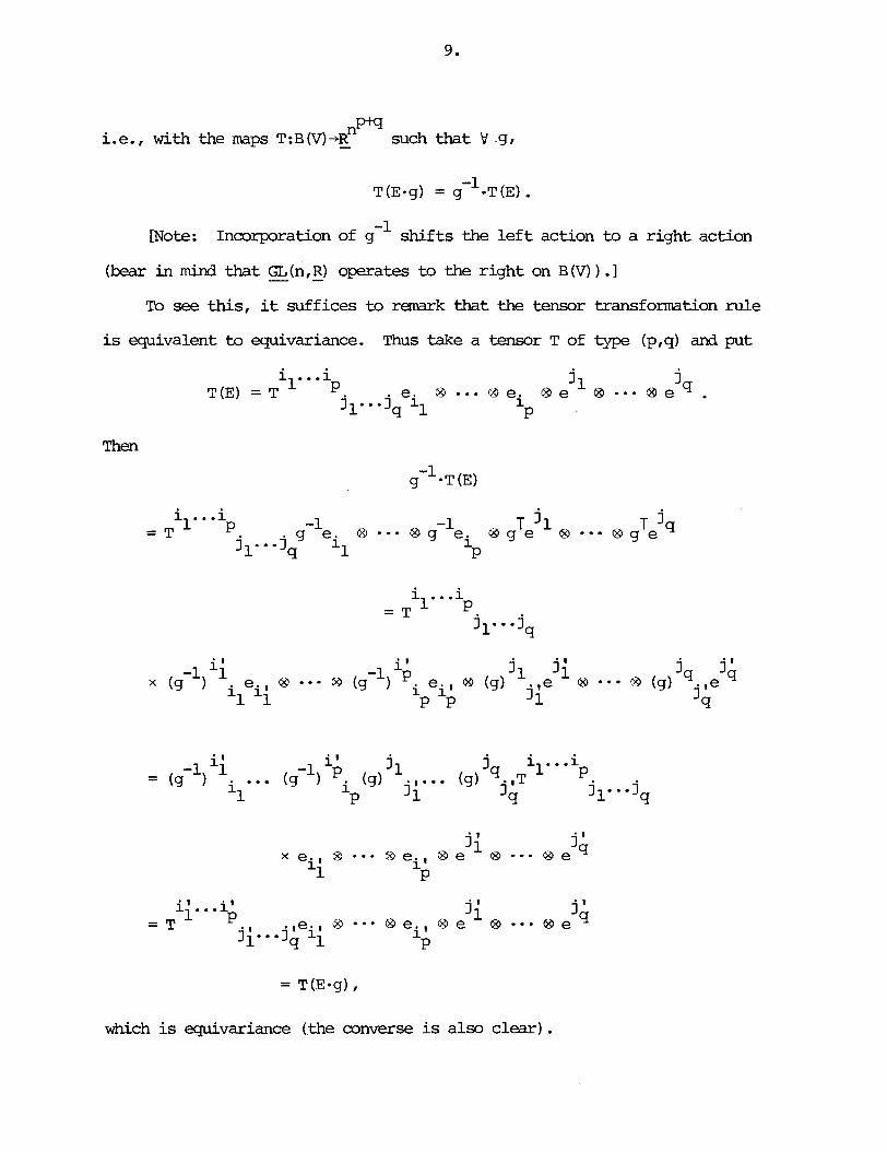
m i.e., with the maps T:B(v)-+R~ - such that V g,

T ( E = ~ ) = 9 - l . ~ (E) . [Note: Inmrporation of sh i f t s the l e f t action to a r ight action

(bear in mind that GL - (n, - R) operates to the right on B (V) ) . I

To see this, it suffices to remark that the tensor transformation rule

is equivalent to equivariance. Thus take a tensor T of type (p,q) and put

= T(E-g) I

which is equivariance (the converse is also clear).

There

situation,

R:gx = x V -

remains one pint of detail , mmly when p = q = 0. In this

rn R" - = - R arad we shall agree that - GL(n,R) - operates t r iv ia l ly on

x€R. - Consequently, the tensors of type (0,O) are the constant mps

0 T: B (V) -t - R, i. e. , Vo = - R (the usual agreement) .

Definition: Let X:GL(n,R) - - -t - $ be a continuous lmmrmrphism -- then a

tensor of type (p,q) and weight X is a map

such that V g,

Special Cases:

1. Tensors of type (p,q) are obtained by taking X (g) = ldet g / O;

2. Twisted tensors of type (p, q) are obtained by taking X (g) = sgn det g .

Rappel: The continuous hommrphisms X :GL - (n,R) - + R' - f a l l into t m classes:

A density is a m p

X:B(V) -t - R

for which 3 rER: - V g,

h(E-g) = ldet g l r X(E) . A twisted density is a map

for which 3 r€R: 'v' g, -

[Note: In either case, r is called the vieight of 1.1

Trivially, tensors of type (0,O) are densities of weight 0.

Example: Suppose that T is a tensor of type (0,2) and weight XI where

X(g) = Idet glr. Define

)tr(E) = det T (E)

r det [Tjlj21.

Then

= ldet glrn detr j 1

ji I

m = ldet gl jl det[(g) ji jlj2 j2

(g) jil

= ldet glr n det gT- det T(E) det g

= ldet glrn (det g) 2 det T(E)

r + 2 = ldet gl g(E)

Therefore is a density of might m+2.

[Note: If T were instead a X-tensor of type (2,O) or (1,l) (X as above),

then the corresponding is a density of weight rn-2 or rn.]

Example (The orientation m) : In B (V) , write E ' -- E iff 3 g€GL - (n,R) -

(det ~ 0 ) : E' = ~ * g . This is an equivalence relation in B(V) and it divides

+ B (V) into tm equivalence classes, say B (V) = B (v)LLB- (v) . Define a map

Then 'd g ,

Or (Egg) = sgn det g-Or (E) . Therefore Or is a twisted density of weight 0.

+ + + [Note: Recall that t m elements El ,E2€B (V) or E;,E;€B- (V) are said

+ + to have the same orientation, whereas tm elements E EB (V) , E-EB-(V) are said to have the opposite orientation.]

Definition: A scalar density is a map

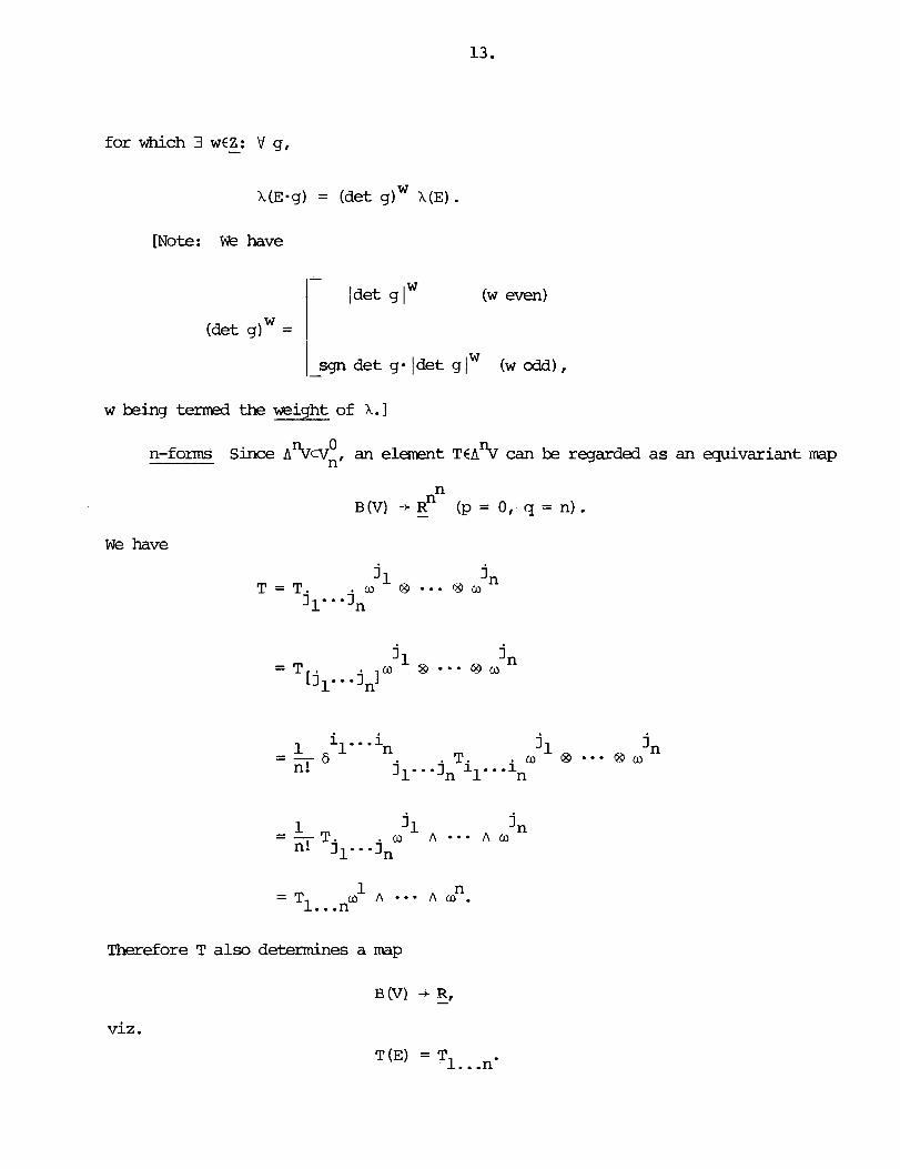
for which 3 w€Z: - tl g,

[Note: W e have

w being termed the might of X.1

n-forms Since A'Gcv~, an elemnt T€A% can bs regarded as an equivariant map

n B(V) -+ - R" (p = 0, q = n).

W e have

Therefore T also determines a map

viz .

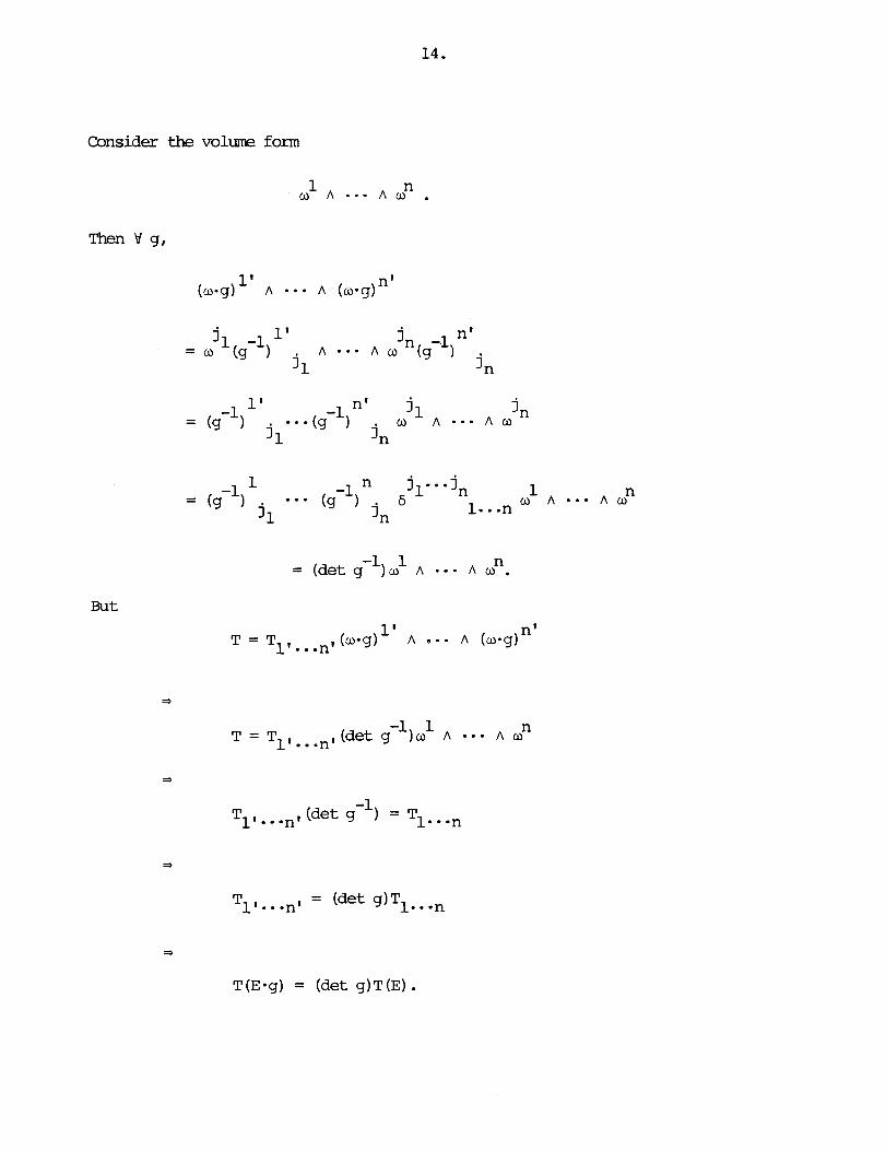
-1 1 n = (det g )a A --• A w . But

=3

-1 1 n = T1l...n'

(det g )a A - - * A o

*

T (Egg) = (det g)T(E) .

Thus i n this way one can attach to each TEA% a scalar density of weight 1.

[Note: Define

1.e.: I T ( is a density of weight 1.1

Definition: The upper Levi-Civita symbol of order n is

and the lower Levi-Civita symbol of order n is

Determinant F o m l a L e t A = [ai. I be an n-by-n matrix - then 3

- il- -in ii n ii.aai' . . .a i n I E det A = E a i n

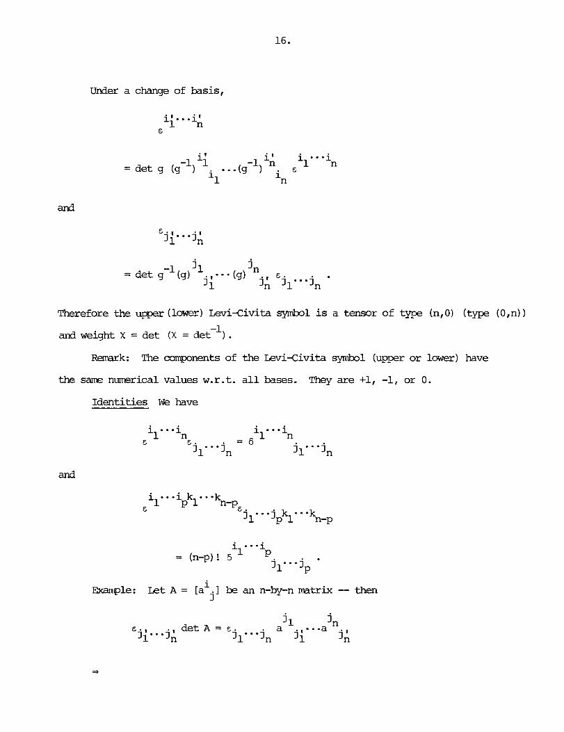
Under a change of basis,

-1 i; i I i .. .i -1 n

= det g (g ) -..(g 1 E 1 n

and

Theref ore the upper (1-1 Levi-Civita symbo3. is a tensor of type (n, 0) (type (0, n) )

-1 and weight X = det (X = det ) .

Remark: The components of the Levi-Civita symbol (upper or lower) have

the s m numrical values w.r.t. all bases. They are +1, -1, or 0.

Identities We have

and

i Dranple: Let A = [a . I be an n-by-n matrix -- then 3

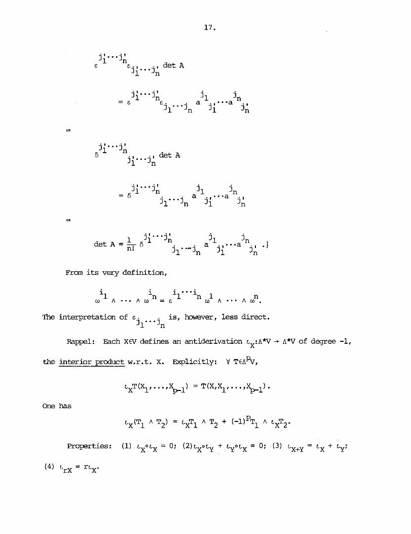
E j i g . .jA E . , det A ji* - 01,

1 V * j A det A = - 6 j 1 j n n! jl* * jn a ji*w*a j A .I

Fram its very definition,

The interpretation of E is, however, less direct. jl* -jn

Rappel: Each XW defines an antiderivation L~:A*V + AW of degree -1,

the interior product w.r . t . X. Explicitly: V TEA%,

properties: (1) = 0: ( 2 ) + L ~ O L ~ = 0; (3) L ~ + ~ = L~ + L ~ ;

Example: By definition,

L e t TCAPV, say

Then

i L (W AT) = (n-p)T.

- Ei

Put

and then set

Proceed £ran here by iteration:

vol = L . . . 1,- *jn E V " ~

j n 3 1

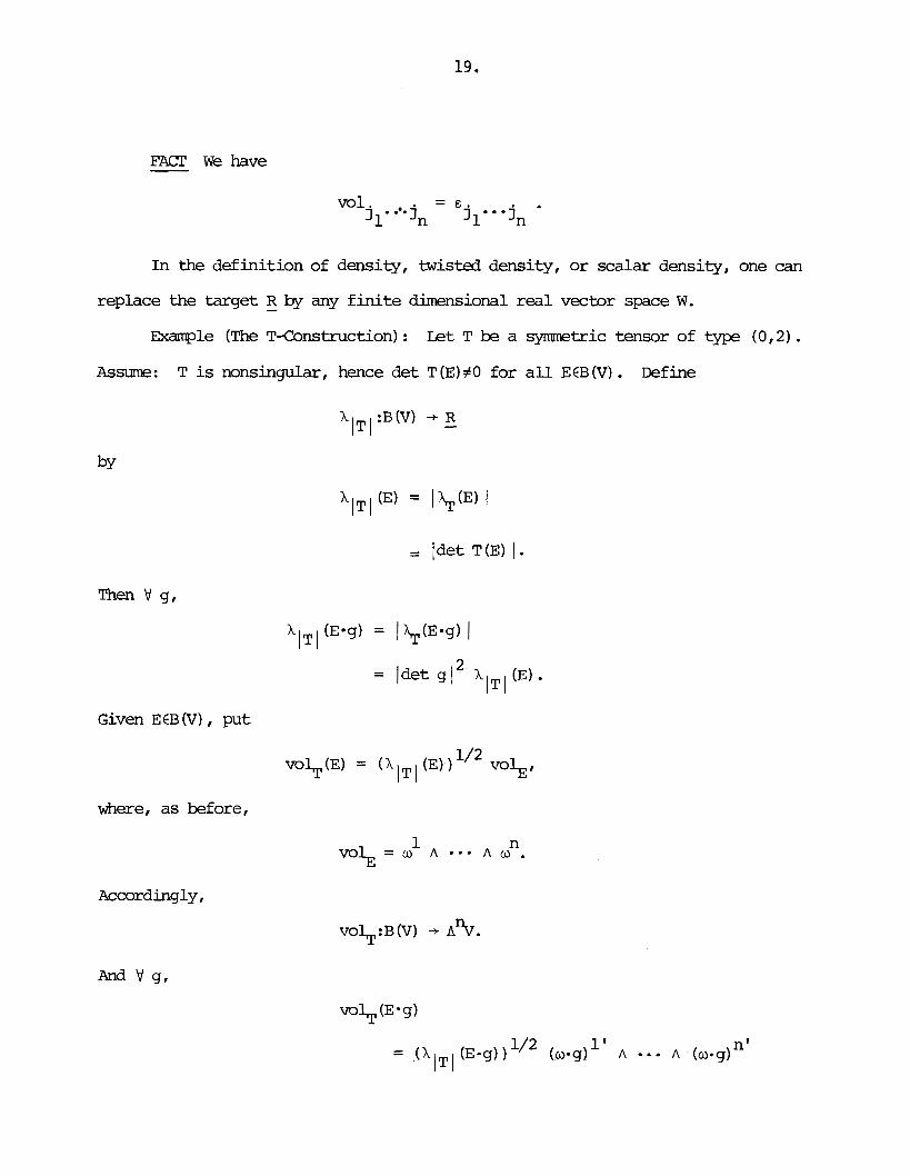
vol - - E j, dn jl--*jn '

In the definition of density, twisted density, o r scalar density, one can

replace the target - R by any f in i t e dimensional rea l vector space W.

Example (The T-Construction) : Let T be a symretric tensor of type (0,2).

Assume: T is nonsingular, hence det T (E) f 0 for a l l EEB (V) . Define

= ldet T(E) I .

Given E CB (V) , put

where, as before,

Accordingly,

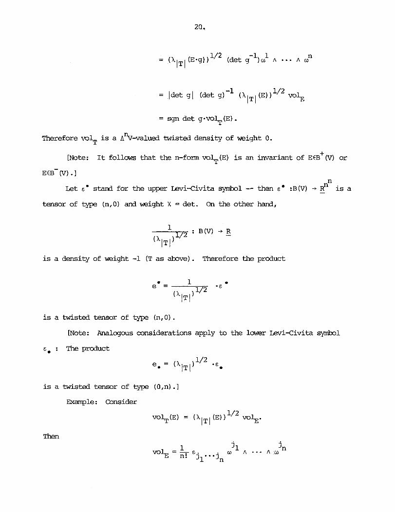
-1 1 n = ( h l ~ ~ ( E * ~ ) ) " ~ (det g )a n --• n o

Therefore voh is a A%-valued twisted density of weight 0.

+ [Note: It follows that the n-form voh(E) is an invariant of EEB (V) or

EEB- (v) . I n

L e t 6. stand for the upper Levi-Civita symbol -- then E :B (V) -t - Rn is a

tensor of type (n, 0) and weight X = det . On the other hand,

is a density of weight -1 (T as above). Therefore the product

is a twisted tensor of type (n, 0) . [Note: Analogous considerations apply to the lower Levi-Civita symbol

E. : The product

is a twisted tensor of type ( 0, n) . I

Example: Consider

V O ~ ( E ) = ( A l T l (E) ~ 0 % .

Then

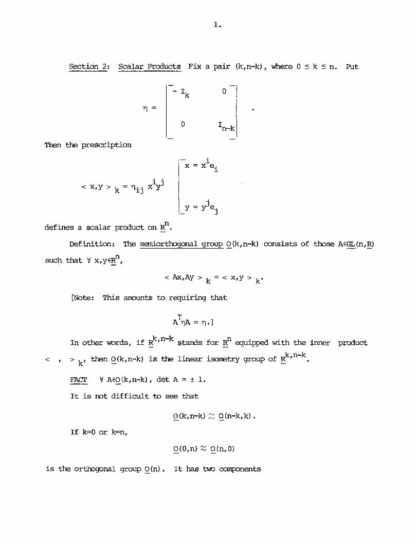
Section 2: Scalar Products Fix a pair (k,n-k), where 0 5 k 5 n. Put

-'I =

Then the prescription

- i j < xly > k - qij Y

defines a scalar product on - Rn.

Definition: The semiorthogonal group - O(k,n-

such that v X , ~ E R ~ , -

.k) consists of those AEGL (n,R) - -

[Note: This arr~unts to requiring that

In other words, i f - R ~ ~ ~ - ~ stands for - R~ equipped w i t h the inner product

k t n-k < 1 > k l then 0 - (k,n-k) is the linear isometry group of R -

FACT VAEO(k,n-k), det A = 2 1. - - It is not d i f f icu l t to see that

O(0,n) 2 g(n,O) -

is the ortbgonal group - O h ) . It has t m corcqpnents

~'(n) = {AEO (n) : det A = '11 I - - -

/ 2- (n) = {AGO - (n) : det A = -11 . I -

Suppose that 0 < k < n -- then O(k,n-k) - has four components

indexed by the signs of det qI, and det AS. Here

with

Definition: The special smiorthogonal group - SO(k,n-k) consists of those

AEO - (k,n-k) such that det A = 1.

Theref ore

is both open and closed in O(k,n-k) . One has -

Remark: By construction, - SO(k,n-k) is the group of orientation preserving

k,n-k + Rk,n-k linear ismetries R d - . On the other hand,

consist of those linear isometrics - R k'n-k -+ - R ~ ~ ~ - ~ that preserve the

- time orientation

- space orientation,

respectively.

[Note: If 0 < k c n, then each of the groups

is of i d e x 2 in - O(k,n-k) .I

Let V be an n-dimensional real vector space -- then a scalar product on

V is a nondegenerate syrm\etric bilinear form

- N .B . Nordegeneracy m u n t s to saying that the rmp gb :V - V* defined by

b g X(Y) = g(X,Y)

is bijective . # [Note: The inverse to g is denoted by g . 1

Therefore g is a symetric tensor of type (0.2) :g€Vo In tenns of a 2 '

1 n basis E = (El,.. . ,E,} €B (V) and its cobasis o = I w , . . . ,o } f B (V*) ,

where

Okservation: The assigrrment

characterized by the condition

-1 b t g (9 x,g Y) = g(X,Y)

is a scalar product on V*.

-1 2 Therefore 9-I is a symetric tensor of type (2,O) :g RTg. And here

where gij is the i jth entry of the matrix inverse to [g . . I , so 13

I;EMMA We have

i i j i j 'In = aet g (E) g 1 ... g n n

E E j1-*-jn -

[Note: In the jargon of the trade, th i s slavs that E * and E are - not

obtained from one a t h e r by the operations of lowwing or raising indices.]

Notation: Given EEB (V) , put

In the T-construction, take T = g -- then

(El = ldetg(E)I = I ~ J J ( E ) 14 1

and, by definition,

1/2 vol (El = ( / g l ( ~ ) ) ~0%. g

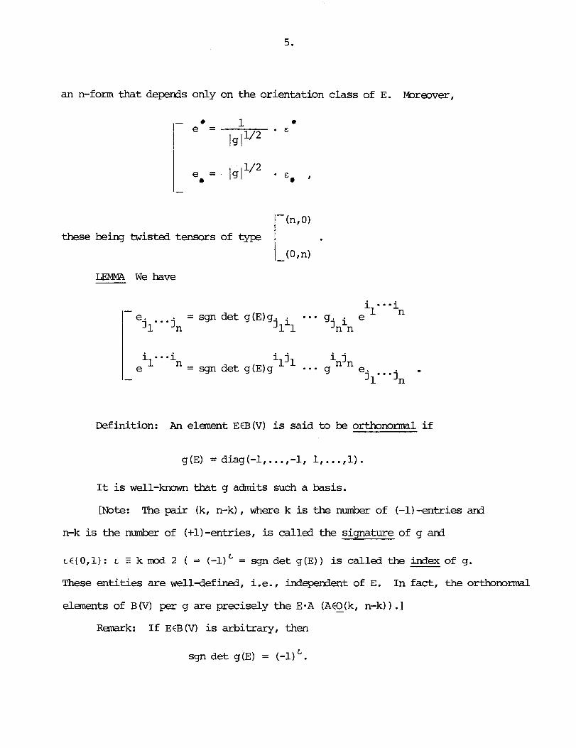
an n-form that depends only on the orientation class of E. mreover,

i i j 1 1 i j 1 e = ign det g(E)g ... g e - j,-jn

these being twisted tensors of type

Definition: An elanent E€B(V) is said to be orthonorr~l if

- (n, 0)

- (0,n)

It is well-known that g admits such a basis.

LEMMA We have

[Note: The pair (k, n-k) , where k is the nLjonbev of (-1)-entries and

n-k is the number of (+l)-entries, is called the signature of g and

tE{O,lI: L E k mod 2 ( (-1)' = sgn det g ( E ) ) is called the index of g.

These entities are well-defined, i.e., independent of E. In fact, the orthonorm1

elements of B(V) per g are precisely the E-A (A€O(k, - n-k) ) . I

R-k: If EEB (V) is arbitrary, then

Let 3, n-k be the set of scalar products on V of signature (k,n-k) -- then

%,n-k ++ B (V) /O - (k, n-k)

or still,

[Note : If E = {El, . . . , E,} CB (V) , then the prescription

defines a scalar product gE@& - having E as an ortl.aonormal basis. -And I

- g~ - 9~-A

for all AEO - (k,n-k) . I

Suppse that g€-Y+ and E€B(V) is orthonormal. Put , n-k

E i = g(Ei,Ei).

Then

LEMMA We have

Remark: If EEB (V) is arbitrary, then

- b - j q Ei - g. .a (E o.) 1 7 1

Ini t ia l ly , we started w i t h a scalar product g on V and then saw how g

induces a scalar product on V*. Pilore is true: g induces a scalar product

g ['I on each of the vP GI q

1 0 -1 [Note: Here, gio1 = g and glll = g - 1

Notation: Given T*, define q

b b = T(g X , . . g Xp,Xpcll.. .,Xpq)

and define

# Components of T :

b Remark: If p = 0, then T = T and i f q = 0, then T# = T.

Fxarcqle: Take T = g -- then

LEM4A The bilinear form

that sends (T,S) to the complete contraction

is a scalar product on vP.

[Note: If g is positive definite, then so is g ['I .I q

From the definitions,

# - b e T @ S Pt4'

Theref ore

# b To c q t e the complete contraction of T sp S , one then sets il = jl,...,i - - Pt4

j ptq and sums the result.

[Note: Take T = g -- then

L e t E€B(V) be orthonormal -- then (2) = 5 i j

Therefore

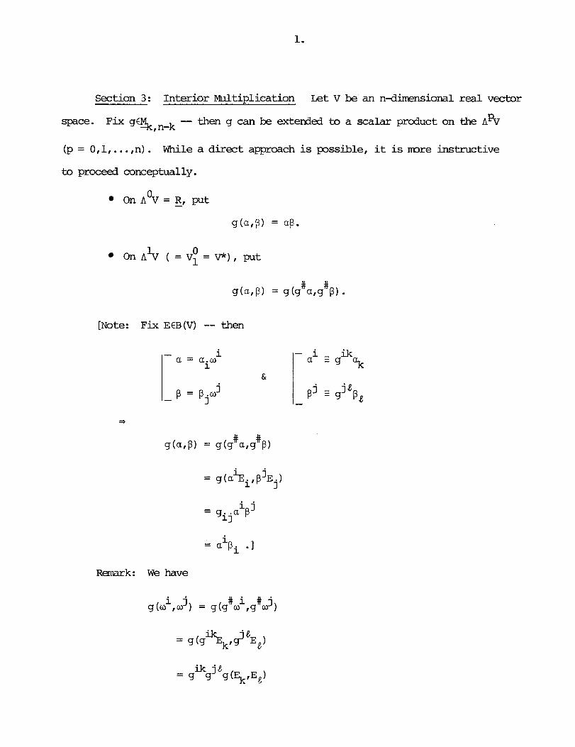
Section 3: Interior Multiplication Let V be an n-dinemional real vector

space. Fix g s , n - k -- then g can be exterded to a scalar product on the A%

( = 0 l . While a direct approach is possible, it is mre instructive

to proceed conceptually.

0 On A V = R, put -

g(a,p) = a@.

[Note: Fix EEB (V) -- then

i = a pi .I

Remark: W e have

i k j = g 6 k

Let q 5 p -- then there is a bilinear map

which is characterized by the following properties:

L - - O L . B1 A Bz '82 @I

0 [Note: One calls I. the interior product on A%. If $En V = RI then -

L~ is simply multiplication by p.1

Remark: 'J x w ,

- tX - Lg b X-

[Indeed,

= g(gbx,g'W tgbX(g Y)

per EEB (v) , write

Put

Let afbPV, @€.A%, where q 5 p -- then

Take q = p -- then c a is a real nmber and we set, by definition, B

g(a,p) = L a = P L ~ B

and g is a scalar product on A%.

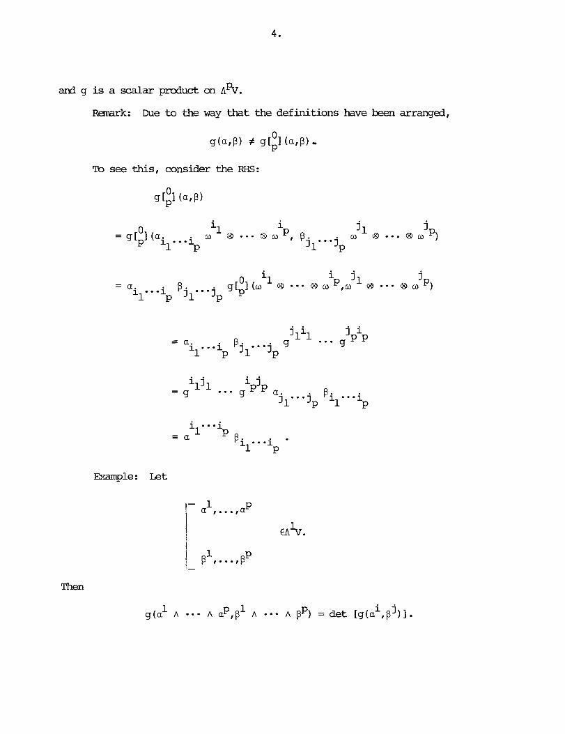
Remrk: Due to the way that the definitions have been arranged,

0 g(a,B) ic g[ I (a,@) P

To see this, consider the RHS:

0 9 Ipl (a.P)

Example: Let

Then

1 i j g(a A --• A aptp1 A - * - A gp) = det [g(a , p 11.

LEMMA Let {Elt...tE 1 be an orthonormal basis for g -- then the collection n

is an orthonorm1 basis for the extension of g to (1 5 p 5 n) . [Note: We have

- 1 1 - 9 - E (no sum)

i j I

Therefore

where P is the n* of indices amng {il,...ti 1 for which .si= -1.1 P

In other mrds, the operations

are mutually ad joint.

Consider now

This n-form depends only on the orientation class of E. Thus there are but t m

possibilities. Pick one, call it an orientation of V, and freeze it for the

ensuing discussion.

N.B. We have

vol = - e 31 j n o A *-• A o . g n! jl-• j n

Definition: The star opesator is the isom3rphism

given by

Theref ore

LEMMA We have

**a = (-1) ' (-1)'' n-P)a .

Observation: L e t ~CA'V, fl €.An% -- then

= C C.pl P Gl

=

= g(*a ,p) . Example: We have

In what fol lws, a€A% and

Rules

0 L *a = * (aAB) . B

[In fact,

L *a = L L ~ V O ~ B P g

= "ApvO1cJ

= * (aAP) .I

fl a% (subject to the obvious restrictions) .

= (-1)' g(a,p)vol .I

Example: Specialize the relation

*L a = (-1) B

q ( n ~ ) * a A p

b and take $ = g X - then

[Write

Then

But

Therefore

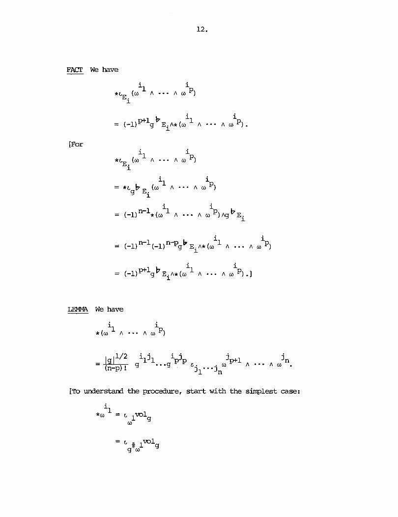
FACT We have

[For i

LE2WA We have

['llo understand the procedure, start w i t h the simplest case:

Now go from here by iteration:

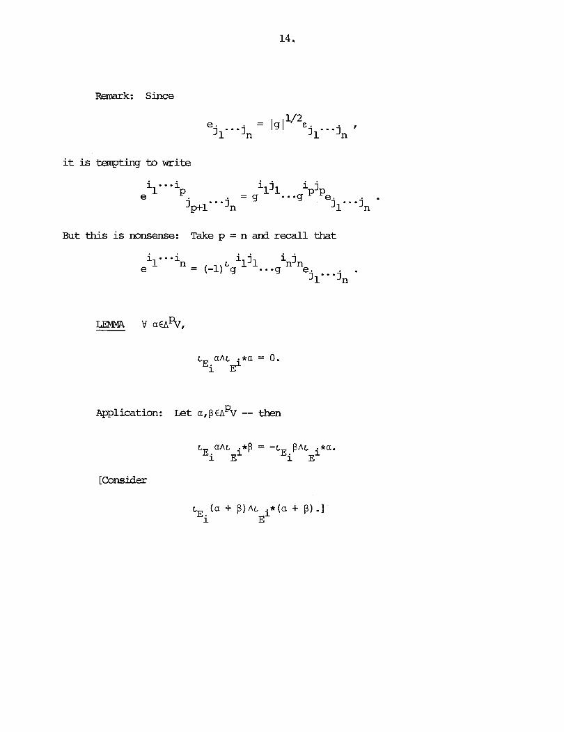
Renark: Since

it is tempting to write

But this is nonsense: Take p = n and recall that

Application: Let a, f3 €A'V -- then

[Consider

Section 4: Tensor Analysis Let M be a connected cm manifold of dimension

n,

0 I [ N o t e : Here, Do (M) = cm (M) , D l (PI) = D (M) , the derivations of cm (M) 0

0 1 (a. k. a. the vector fields on M) , and Dl (MI = Dl (MI the linear f0n-r~ on D (M)

viewed as a module over cm (M) ) . I

Remark: By definition, DP(M) is the cm(M) -mdule of a l l cm(M) -multilinear q

One can also interpret the e l m t s of vP(M) g m t r i c a l l y . To this end, consider q

the frame bundle

W h k h g of - R" as merely a vector space (and not a s a m i f o l d ) , let %(n) be

the tensors of type (p,q) -- then - GL (n,R) - operates to the l e f t on @ (n) (cf . q

Section 1). Now form the vector bundle

Then, on general grounds, there is a one-to-one correspondence betmen the

sections T of T' (M) and the equivariant maps @:LM -+ (n) q

Of course, as a set

hence Q = {+x: x€Ml , where

And we have

or still,

[Note: One advantage of the geometric point of view is that it can be

readily generalized, e. g . , to tensors of type (p, q) a d weight X .I

Details Given (x, E) CIM ( 3 E CB (TxM) ) , define %:Rn - + TxM by

Then V gGL - (n,R) - , the canpsi te - Rn 2 - Rn ? T N is H.g . X

T + QT: This is the arrow

Q -+ TQ: This is the arrow

where

FACT These arrows are mutually inverse:

In what follows, all o ~ a t i o n s will be defined globally. However, for

computational purposes, it is important to have at hand their local expression

as well, meaning the form they take on a connected open set UcM equipped with

1 n coordinates x ,..., x . Let TE%(M) -- tlw locally

where

are the caqonents of T.

Under a change of coordinates, the components of T satisfy the tensor

transformation rule:

[Note: Thexe are maps

viz .

FACT Equip ~ ' (n) with its standard basis -- then 9

we have

Ranark: Suppose there is assigned to each U i n a coordinate at las for M,

functions

subject to the tensor transformation rule -- then there is a unigue T€ fl (M) q

d s e cmpnents in U are the T j1- -jq0

[It is simply a mtter of manufacturing a global section of T'(M) by 9

gluing together local sections.]

Exarc-p?le: The Kronecker tensor is the tensor K of type (1,l) defined by

K(A,X) = A (X) , thus

i a i K~ = K(dx , 7) = 6

j ax3 j '

FACT There is a tensor K(p) of type (p,p) with the property that i n any - coordinate system,

Notation: Given f €cm (u) , write

[Note: The bracket

1 1 [ , 1 : D1(m x v (MI + D (MI

is - R-bilinear but not c"l (M) -bilinear. In fact,

Definition: A type preserving - R-l inear nap

which comrmtes w i t h contractions is said to be a derivation if Y T1,T2€D(M),

[Note: To say that D is type preserving means that D@ (M) c@ (M) . ] q q

The s e t of all derivations of D(M) forms a L i e algebra over R, the bracket -

operation being defined by

[D1,D2] = Dl 0 D2 - D2 Dl.

R-k: For any £ E C ~ ( M ) and any TED(M), fT = f 63 T, so D(£T) = f (DT)

+ (Df) T. In particular: D is a derivation of cm (M) , hence is represented on

ern (M) by a vector field.

Construction: L e t

Then Y xCM,

Ax:TxM + TxM

is - R - l i n e a r , hence can be uniquely extended to a derivation D of the tensor Ax

algebra over TxM. This said, define

DA:Q(M) + D(M)

Then DA is a derivation of D (M) which is zem on cm (M) .

FACT Any derivation of D(M) which is zero on c-(M) is induced by a tensor - of type ( 1 , l ) .

1 [Note: If D is a derivation of D (M) and if AED1 (MI , then [DIDA] IcW (MI = 0 ,

1 1 hence [DIDA] = DB for scnne B C D ~ (M) . Therefore Dl (M) is an ideal in the ~ i e

algebra of derivations of P (M) . I Product Formula Let D:D(M) - D(M) be a derivation -- then V T€<(M),

1 [Note: This shows that D is known as soon as it is known on c-(M) , D (M) ,

and Dl (M) . ~ u t for o€D1 (MI .

thus functions and vector fields suffice.]

FACT Let D1,D2 be derivations of D(M). Assume: Dl = D~ on c-(M) and

ol (MI -- then Dl = D2.

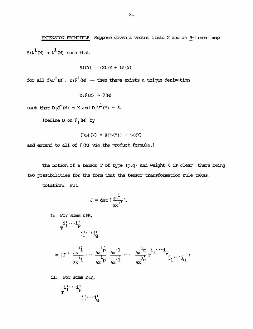
EXTENSION PRINCIPLE Suppose given a vector field X and an - R-linear map

1 1 6 :P (M) -t P (M) such that

6 (£Y) = (X£)Y + £6 (Y)

1 for all f € c W ( ~ ) , YEP (M) -- then there exists a unique derivation

1 such that DIC-(M) = X and D I D (M) = 6.

[Define D on Pl(M) by

The notion of a tensor T of type (p,q) and weight X is clear, there being

ts.m possibilities for the form that the tensor transformation rule takes.

Notation: Put

i ax J = det [ -1. axi '

I: For some rER, -

11: For sane r € R , -

Accordingly, there are t m kinds of tensors of type (p,q) and weight X I

which we shall refer to as class I and class 11. It is also convenient to single

out a particular carbination of these by an integrality condition.

Definition: A tensor of type (p,q) and weightw is a tensor T of type

(p,q) and weight X = (detlW (w€Z-1 , hence

[Note: Needless to say, the tensors of type (p,q) and weight 0 are

precisely the elements of 04 . I q

Remark: The product of a tensor T of type (p,q) and weight w with a

tensor TI of type (pl ,q ' ) and weight w' is a tensor T @ T' of type (p + p', q + q')

and weightw + w'.

E q l e : The upper Levi-Civita symbol is a tensor of type (n,O) and

weight 1 and the lower Levi-Civita symbol is a tensor of type (0,n) and weight -1.

[To discuss the upper Levi-Civita symbol, write

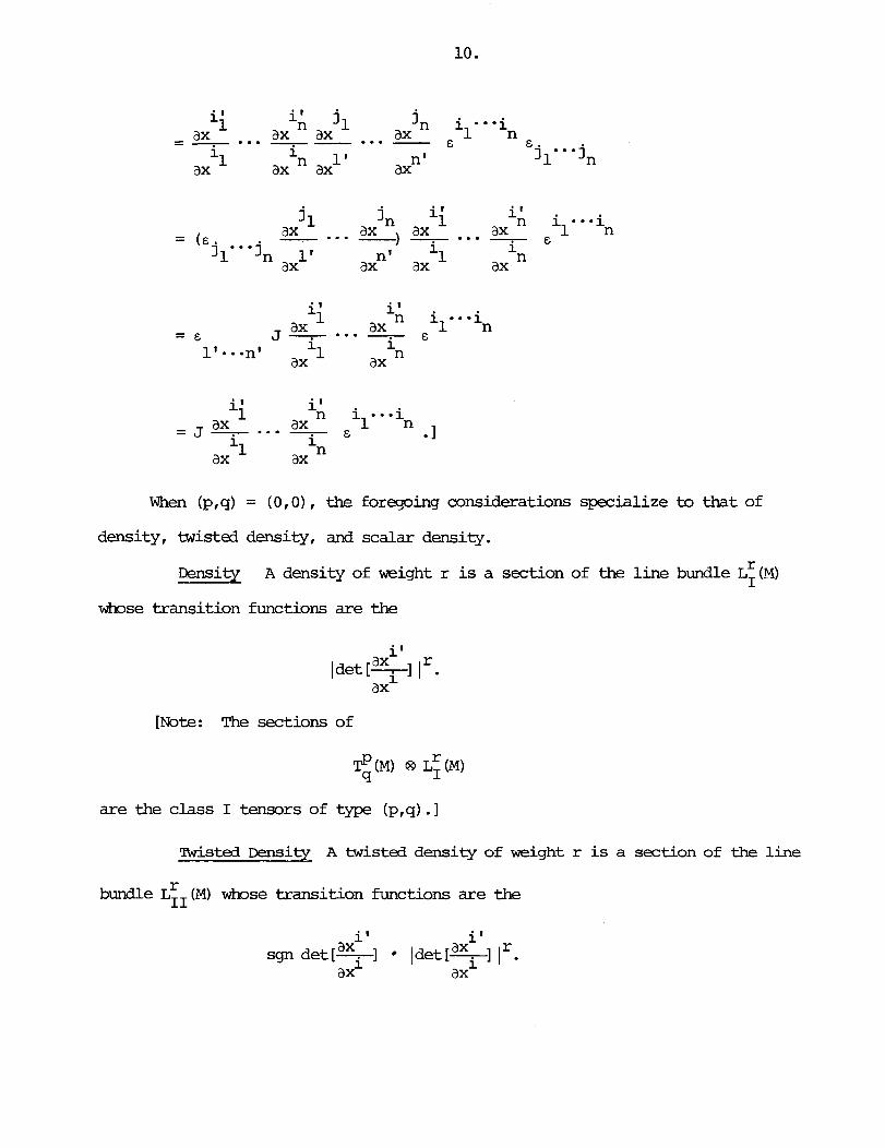
When (p,q) = (0,0), the foregoing considerations specialize to that of

density, twisted density, and scalar density.

Density A density of weight r is a section of the line bundle L: (M)

whose transition functions are the

[Note: The sections of

misted D e n s i t y A twisted density of weight r is a section of the line

bundle L:=(M) whose transition functions are the

i ' i ' ax r sgn det [--I ~det [%I / .

ax1 ax

[Note: The sections of

are the class I1 tensors of type (p,q) -1

Scalar Density A scalar density of weightw is a section of the l ine

bundle L~(M) whose transition functions are the

[Note: The sections of

are the tensors of type (p,q) and weight w. 1

Exanple: The density bundle is the l ine bundle

whose transition functions are the

ax" Idet [-I I . ax1

Therefore

1 Lden (MI = LI (MI

m l e : The orientation bundle is the l ine bundle

whose transition functions are the

ax" sgn det [-I . 1 ax

Therefore

0 Or (M) = LII (M) .

mample: The canonical bundle is the line bundle

whose transition functions are the

ax" det [-I .

Therefore

1 Lcm (M) = L (M) .

Remark: The canonical bundle can be identified with A%*M, where T*M

is the cotangent bundle. Since

it follows that the n-forms on M are scalar densities of weight 1.

[Note: The upper Ievi-Civita symbol is a section of

and the lower Levi-Civita symbol is a section of

Section 5: L i e Derivatives Le t M be a connected cm manifold of

dimension n.

1 LIDMA One may attach to each XED (M) a derivation

called the Lie derivative w.r. t . X. It is characterized by the properties

1 [In the notation of the Extension Principle, define 6: 4 (M) + d. (M) by

6 (Y) = [X,Yl . Then

Owing to the product formula, V T E$ (PI) , 9

1 P X [ T h A I X I I - - * , X ) I

9

[Note: If otD1 (MI , then

[Note: From the definitions,

At a given x€M, the expression

can be explained in terms of the canonical representation p of - GL (n,R) - on *(n) q

or, m r e precisely, its differential dp.

Tb see this, fix for the mment an elanent ~€'l?(n) -- then V g€GL(n,R), q - -

Now pass IXI the derived mp of Lie algebras

and we have

a Returning to M, use the basis { -

ax x

to identify TxM with R", - thence T'T M with $(n) . Put q x

i i A . (x) = - X . (x) .

3 r I

Remark: The symbol

is usually abbreviated to

Example: Let K be the Kronecker tensor -- then

[Note: In general, V p1,

q ' p ) = 0.1

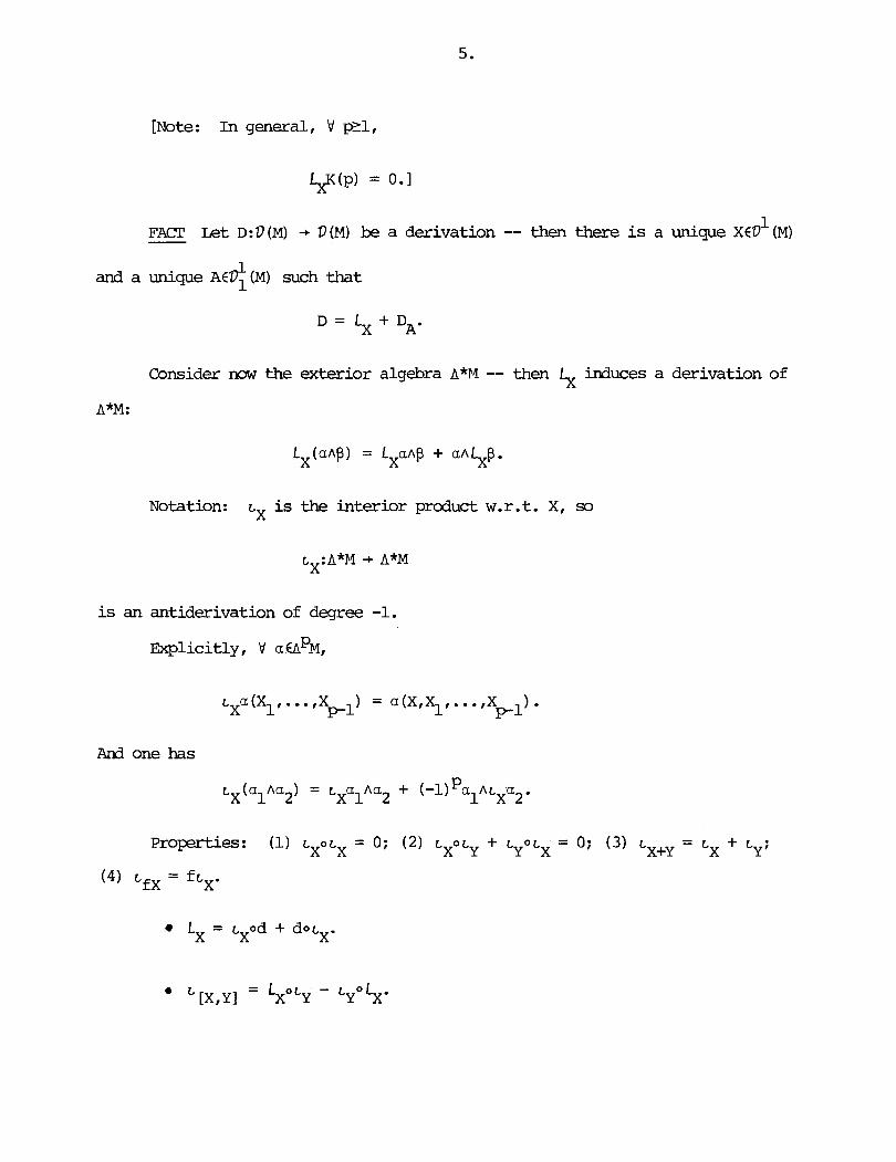
FACT - Let D:D(M) + D(M) be a derivation -- then there is a unique x€D'(M)

and a unique A C D ~ (M) such that

D = L + DA. X

Consider now the exterior algebra A*M -- then 5 induces a derivation of A*M:

Notation: tX is the interior product w.r.t. X, so

is an antiderivation of deqree -1.

FXplicitly , V a a P M ,

And one has

properties: ( 1 ) cX0cX = 0: (2) + L o e = 0; (3) L ~ + ~ - Y X - Cx + cy;

(4) L f X = ftX.

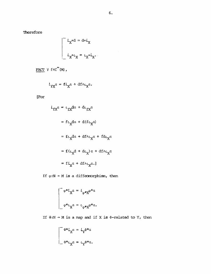
Therefore

[For

= fCXda + d c f ~ ~ a )

= f~ da + dfAtxa + fdCXa X

= f ( ~ ~ d + d ~ ~ ) a + dfnLXa

= £9 + d f n ~ ~ a . ]

If q:N -+ M is a di f£mrphism, then

If @:N -+ M is a map and if X is @-related to Y, then

[Note: Recall that

are said to be @-related if

or, equivalently, if

Y (fa@) = H o +

Denote by w-9 (M) the tensors of type (p , q) and weight w -- then q

Put

1 FACT One may attach to each XED (M) a type preserving R-linear map -

LX:W-V (M) -+ W--D (M)

called the Lie derivative w.r.t. X. Locally, LXT has the same formas a tensor

of type (p,q) except that there is one additional term, namely

[Note: If

then

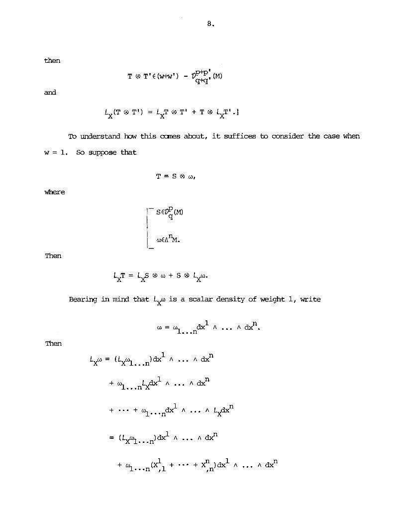
and

To understand how t h i s caws about, it suffices to consider the case when

w = 1. So suppose that

Bearing i n mind that Lf is a scalar density of weight 1, write

Then

1 + y L d x A ... A d x " . . .n X

Therefore

Example: L e t T be the upper Levi-Civita symbol (a tensor of type (n, 0)

and weight 1) or the lowex Levi-Civita symbol (a tensor of type (0,n) and

weight -1) -- then LxT = 0.

[To discuss the upper Levi-Civita symbol, mte that

[Note: The t e r m s involving three identical *ices are not surrpned.1

Given wEZ, - let pw = (de t IYYp and consider the derived rmp of L i e algebras

Then V AEgE - (n, - R) ,

= -w tr (A) + d p (A) .

Put

i i A . (x) = -X . (x)

3 13

and let T€W-@ (M) -- then at x, q

Section 6: Flows L e t M be a connected cm inanifold of dimension n.

1 Fix an XED (M) -- then the image of a maximal integral curve of X is called

a trajectory of X. The trajectories of X are connected, imersed sul.mrranifolds

of M. They form a partition of M and their dimension is either 0 or 1 (the

trajectories of dimension 0 are the points of M where the vector f ield X vanishes).

Definition: A f i r s t integral for X is an f €cW (PI) :Xf=O.

In order that f be a f i r s t integral for X it is necessary and sufficient

that f be constant on the trajectmries of X.

Recall now that there exists an open subset D ( X ) ~ R x M and a differentiable - function o ~ : D ( X ) + M such that for each x€M, the map t -r OX(tIx) is the trajectory

of X w i t h 6x(0,x)=x

is an open interval containing the origin and is the domain of the trajectory

which passes through x.

is open in M and the map

+t,X -+ 4Jxtt,x)

is a dif f eomrphism Dt (X) -r D-t (X) with inverse 4J -t'

(3) I f (t ,x) and ( ~ , + ~ ( t , x ) ) are elanents of D(X) , then (s+t,x) is an

element of D (XI and

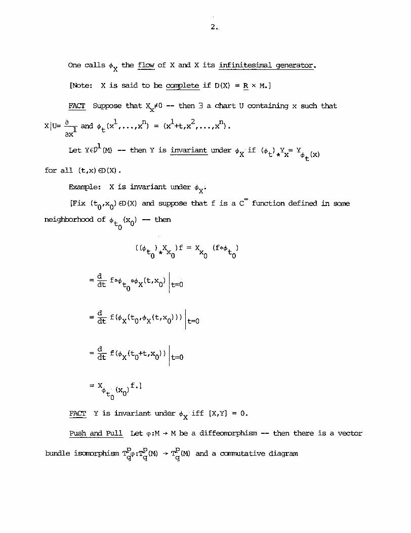
One ca l l s bX the flow of X and X its infinitesimal generator. -

[Note: X is said to be ccarrplete i f D(X) = - R x M.]

FACT S u p s e that Xx#O -- then 3 a chart U containing x such that

a 1 n 1 2 n X/U= - and 4t(x .....x ) = ( x +t.x ..., x ) . ax 1

Let Y€+(M) -- then Y is invariant wder 4x i f ( 4 ) Y = Y t * x +,(XI

for a l l ( t , x ) ED (X) . Example: X is invariant under 4 x- [Fix ( t0 .x0) €D(X) and s u p s e that f is a C- function defined i n sane

neighbor- of 4 (x0) -- then

FACT Y is invariant under OX i f f [X.Y] = 0. -

Push and Pull L e t cp:M -t M be a diffecnmrphism -- then there is a vector

bundle isom~rphisn T$p :T'(M) -+ $ (M) and a camatative diagram q

the pushforward of T.

[Note: Thus

q*T = ~ q - l o ~ o q . q

the pu l lback of T.

[Note: Thus

q* = -1 (cp ) *

The standard fact that

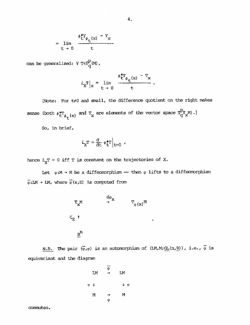
L = l im

t - + O t

can be generalized: tl TE$(M), q

CT4,tX) - Tx L T = lim

lx t + O t

[Note: For t # O and small, the difference quotient on the right makes

So, in brief,

hence L T = 0 i f f T is constant on the trajectories of X. X

L e t cp :M -t M be a diff eormrphism -- then cp l i f t s to a dif feormrphisn

- cp:M -t IM, where T(x,E) is computed from

- N.B. The pair (7,cp) is an automrphisn of (LM,M;GL(~ ,R)) , i.e., cp is - -

equivariant anli the diagram

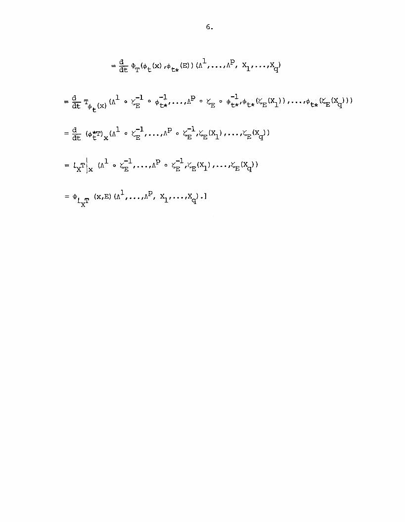
O b s e r v a t i o n : W e have

- + cp*T

[In fact,

- 1 P QT O lp(x,E) (A ,..., A , X1,...,X 1 q

L e t x€$ (MI -- then gX lifts to a f l o w T on IM. - v

LJ3Wi We have

[At t = 0,

Section 7 : Covariant Differentiation Let M be a connected C- manifold

of dimension n. Suppse that E -+ PI is a vector bundle -- then a connection V on E is a map

such that

[Note: By definition, V s is the covariant derivative of s w.r.t. X.] X

Rappel: There is a one-to-one correspondence

between the mnnections I' on the £ram bundle

and the connections V on the tangent bundle

Let con TM stand for the set of connections on TM.

0 Let V€ con avl -- then the assignment

is not a tensor.

Let V1,V"E con TM -- then the assignment

L e t V E con TM

hence is a tensor.

I (XIY) -t VXY + +(X,Y) -

is a connection.

I Scholim: con 1M is an affine space with translation group P2(M).

[The action V Y = V + Y is free and transitive. 1

Remark: Write con LM for the se t of connections on LM -- then, on general

grounds, con LM is an affine space (in the 1-form description, the translation

Let V be a connection on TM. Put V X f = Xf and i n the notation of the

Extension Principle, take 6 = VX (permissible, since Vx(fY) = ( X f ) Y + fVxY) -- then there exists a unique derivation

1 such that V ~ I C ~ ( M ) = X ard vx1D (M) = 6.

1 [Note: The difference Vx - L is cm (M) -linear on D (M) : X

= (Xf)Y + fVXY -

= f(VXY - LXY) ,

hence V as a derivation of P (M) X

(xf)Y - fLXY

admits the decomposition

Remark: Write V = vr -- then r induces a connection

and matters are consistent:

1 On general grounds, each XED (M) admits a unique lifting to a horizontal

vector field Xh on IM such that IT,$ = X.

FACT We have

Owing to the product formula, Y T C% (M) ,

1 n Definition: Let V be a connection on 'I?!!. Suppose that (U,{x ,..., x ) )

is a chart -- then the connection coefficients of V w.r . t . the coordinates

xl, . . . ,xn are the C- functions lkij on U defined by the prescription

Observation: V X C V ~ (M) ,

So locally,

RaMlrk: The symbol

is usually abbreviated to

Exarrq?le: L e t K be the Kronecker tensor -- then

Indeed,

[Note: In general, V pl ,

DMMA Let V be a connection on TM -- then on UCIU',

[Note: This relation is called the connection transformation rule.]

Therefore the rkij are not the canpnents of a tensor.

FACT Assume that there is assigned to each U in a coordinate at las for MI

functions

subject to the connection transformation rule -- then there is a unique

connection V on TM whose connection coefficients w.r.t. the coordinates

1 n x ,..., x are the I' k ij

j Rsmrk: Consider the contraction I' ij. To determine its transformation

law, write

Then

On the other hand, by determinant theory,

[Note : Analogously,

Let V be a connection on 'IIM -- then V induces a m p '@(MI -+ (M) , viz. 9 9+1

1 VT(A ,..,A~, X1,...,X ,X)

q

[Note: One calls VT the covariant derivative of T.]

Working locally, put

where

Then i n view of what has been said above,

[Note: The cmnpnents of VT are the

Thus

where

nark: Wc TC%(M) -- then T is said to be parallel if VT = 0, which is

the case i f f VXT = 0 for a l l X d ( M ) .

Notation: Define vk: DP (MI -+ DP (MI by v1 = v arii vk = v (vk- l ) ( b 1 ) . q s+k

[Note : V ~ T c % + ~ (M) and

is written as

or still, il--=i

'bVaT P .I j1*-*jq

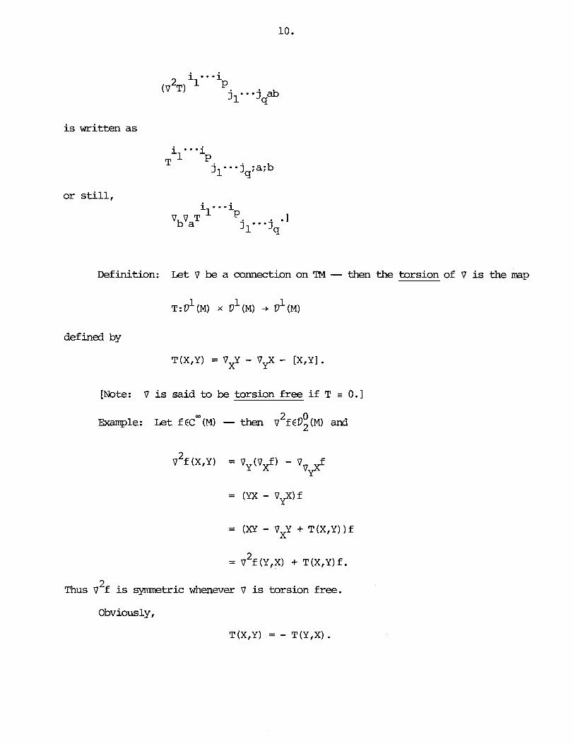
D e f i n i t i o n : L e t V be a connection on TM -- then the torsion of V is the mp

defined by

T (X,Y) = VXY - V$ - [X,Y] .

[Note: V is said to be torsion free i f T t 0.1

2 0 m l e : L e t £ CC- (I) -- then V f €02 (14) and

2 = V f ( Y , X ) + T ( X , Y ) f .

2 Thus V f is syrmnetric whenever V is torsion free.

O b v i o u s l y ,

T(X,Y) = - T (Y,X) .

It is also easy to check that

Therefore the assigrnnent

is a tensor, the torsion tensor attached to V .

Construction: Given V E con TM, define V 1 € con TM by

V ' = V - T.

This makes sense (recall that con TM is an affine space w i t h translation group

1 D 2 ( M ) ) . To compute the torsion of V ' , note t h a t

Therefore the connection

is torsion free and

Finally, suppose that

where 7 is torsion free and

subject to

S(X,Y) = - S(Y,X).

Then the torsion of V is the torsion of ? plus

- 1 v = - 1 v + 2 v ' .

Pbrking locally, write

a a a T(-r -) = - ax' ax7 ij axk

Then

[Note: Consider the decomposition

1 1 1 V = (?V +-8') +-T. 2 2

Then, in terms of connection coefficients,

Example: L e t fccm (M) -- then

2 a a 2 a a a v f(- r-1 = v I--) + T(--T I---)£ axi 8x3 axj ax' ax1 3x3

or still,

Let TED' (MI -- then q

On the other W,

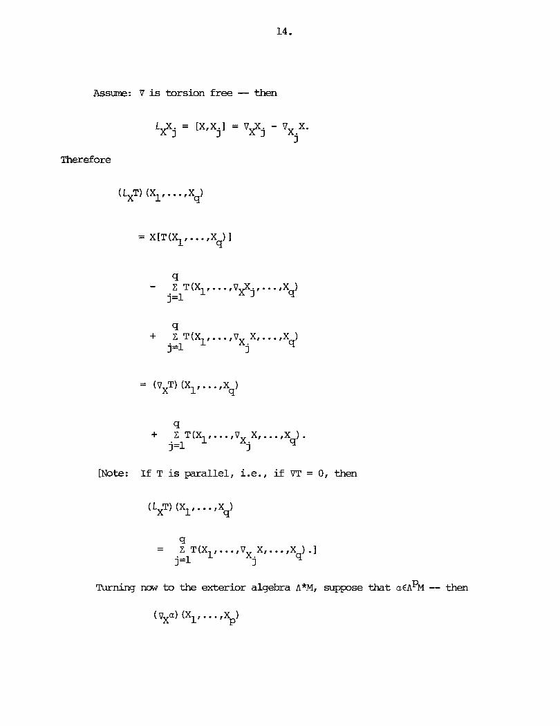
Assume: B is torsion free -- then

Therefore

[Note: If T is parallel, i.e., if VT = 0, then

Turning now to the exterior algebra A*M, suppose that a € n P ~ -- then

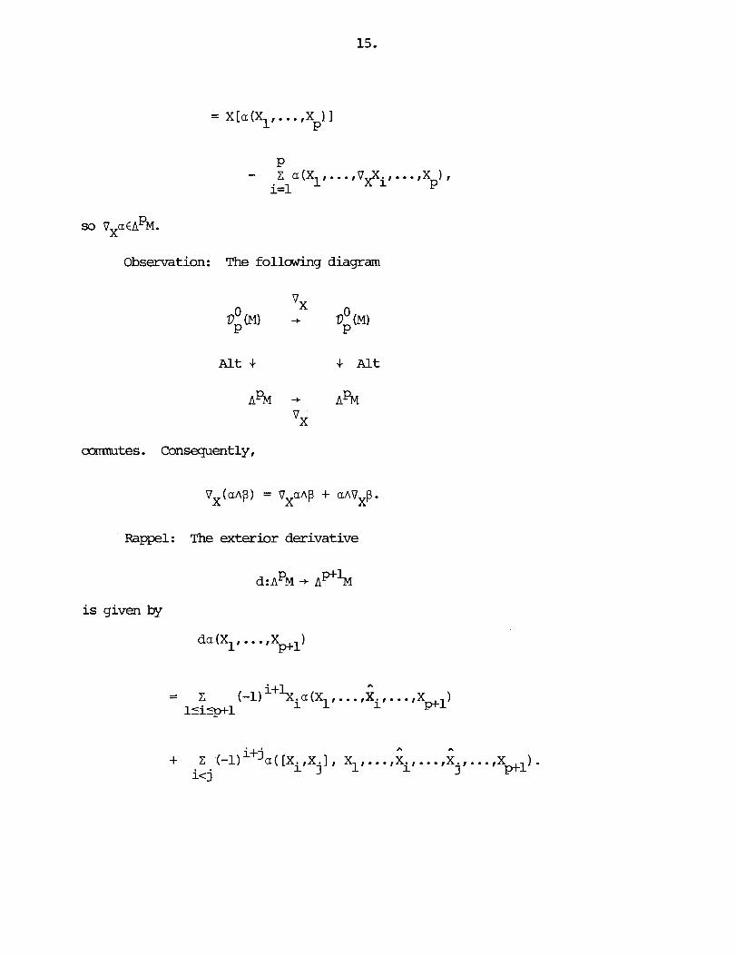
P so VXaEA M.

Observation: The following diagram

ommutes. Consequently,

V (a~p) = V aAg + aAVxp. X X

Rappel: The exterior derivative

~ : A P M + P+lM is given by

There is a triangle

but d#Alt o V.

Ll3M4 Suppose that V is torsion free -- then on A'M,

[ N o t e : Under the assumption that V is torsion free, 'd a tb?~ , we have

thus loca l ly

E.q., take p = 1 -- then

d a ( X , Y ) = Va(Y,X) - Va(X,Y) ,

thus V a is m t r i c i f f a is closed.]

FACT Let X , Y C D ~ ( M ) -- then

L e t I? be a connection on IM. S u p s e t h a t p is a representation of

GL (n,R) on a f in i te dimensional vector space W. Form the vector bundle - -

Then I? induces a connection on E.

Specialize and take W = @(n). p = % -- then one m y attach to each q

~ € 0 1 (M) a mvariant derivative

Lmally, VXT has the same form as a tensor of type (p,q) except that there is

one additional t e r m , namely

[Note: If

then

and

Vx(T W T ' ) = VXT W T' + T C3 VXT1.]

Remark: Given w€.A%, write

dxl A - - - A dxn. a = W l . . .n

Then

Example: Let T be the upper Levi-Civita symbol (a tensor of type (n,O)

and weight 1) or the lower Levi-Civita symbol (a tensor of type (0,n) and

weight -1) -- then VxT = 0.

[To discuss the upper Levi-Civita syrtbol, mte that

i ...i = xa" 1 n

I a

i 1 b i 2 - - - i i n i b + xar a n %"' n-1 + - * * + X r

ab"

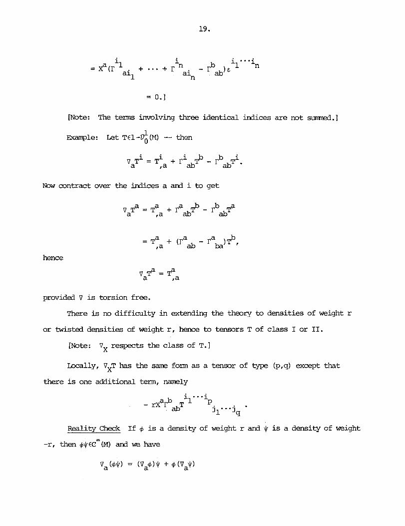
= 0.1

[Note: The terms involving three identical indices are not sunsned. I

1 m l e : Let Tcl-DO(M) -- then

Now contract over the indices a and i to get

hence

provided V is torsion free.

There is no difficulty in extending the theory to densities of weight r

or twisted densities of weight r, hence to tensors T of class I or 11.

[Note : VX respects the class of T. I

Locally, VxT has the same form as a tensor of type (p,q) except that

there is one additional term, namely

Reality Check If 6, is a density of weight r and $ is a density of weight

-r, then +$€ern (M) and we have

Exarrq?le: If + is a scalar density of weight 1 and 9 is a density of

weight -1, then ++ is a twisted density of weight 0 and

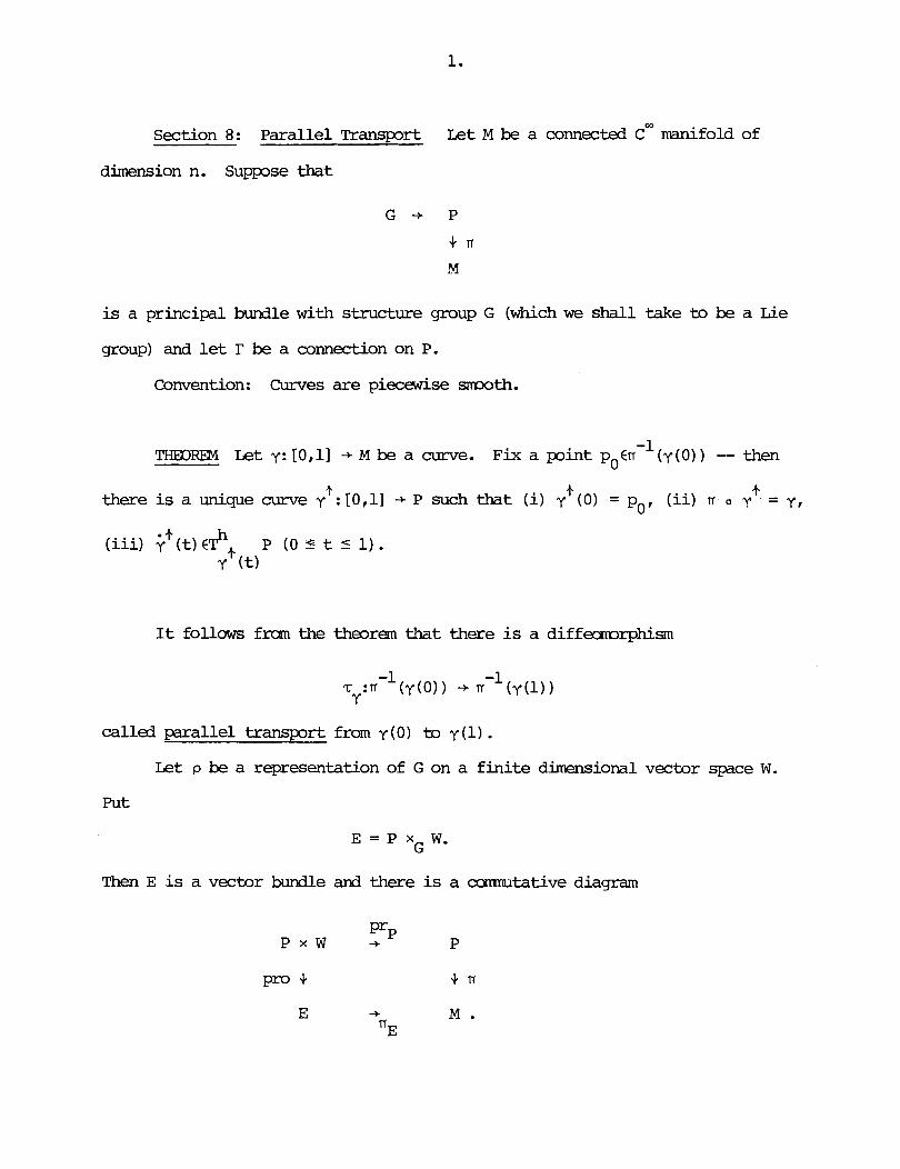
Section 8: Parallel Transport L e t M be a connected cm manifold of

dimension n. Suppose that

is a principal bundle with structure group G (which we shall take to be a L i e

group) and let T be a connection on P.

Convention: Curves are piecewise m t h .

-1 THmIlPM Let y:[0,11 + M be a curve. Fix a point po€n ( ~ ( 0 ) ) -- then

+ + there is a unique curve y': [0,11 + P such that (i) y (0) = po, (ii) n . y = y,

It follows f m the theorem that there is a d i f f ~ r p k i s m

called parallel transport from y (0) to y (1) . L e t p be a representation of G on a f in i t e dimensional vector space W.

Put

Then E is a vector bundle and there is a conmutative diagram

H e r e

nE( [p,wI = n (p) . -1

L e t eo€E. Take any point (po.wo) €pro (eo) and define

Set

Then E is independent of the choice of (pO ,wO) and is called the horizontal 0

subspace of T E (per the cbice of I?) . eo

-1 TJADRl34 L e t y: [O,ll - M be a curve. Fix a pint eOtnE (y(0)) -- then

t t there is a unique curve yt: [O,ll -r E such that (i) y (0) = eo, (ii) nE o y = y,

It follows from the theorem that there is an i m r p h i s n

called para l le l transport from y (0) to y (1) . r 1 Denote by V the connection on E determined by r. Fix xcM and let XED (M) .

choose any curve y: [-E,EJ - M such that y(0) = x and +(o) - - xx . W i f y the

rotation and write

-1 -1 -T -n (~(0)) + n E (y(h)) h' E

for the parallel transprt from y (0) to y (h) .

Specialize to P = LM ard W = $(n) -- p, these generalities are applicable to the

replacing p by p to the sections of $(M) w' q

then, with the obvious choice for

sections of T~ (M) , i .e. , to % (M) , or, q

Section 9: Curvature Let M be a connected coo manifold of dimension n.

Definition: kt V be a connection on TM -- then the curvature of V is

the map

1 1 R&M) x -+ H?(D (MI ,D (MI)

-

def ind by

R(X,Y) = VXVy - VyVX - V [XrYI '

Obviously,

R(X,Y) = - R(Y,X) . It is also easy to check that

Therefore the assignment

is a tensor, the curvature tensor attached to V.

Ranark: The Lie derivative LXV of the connection V is the cW (M) -multilinear

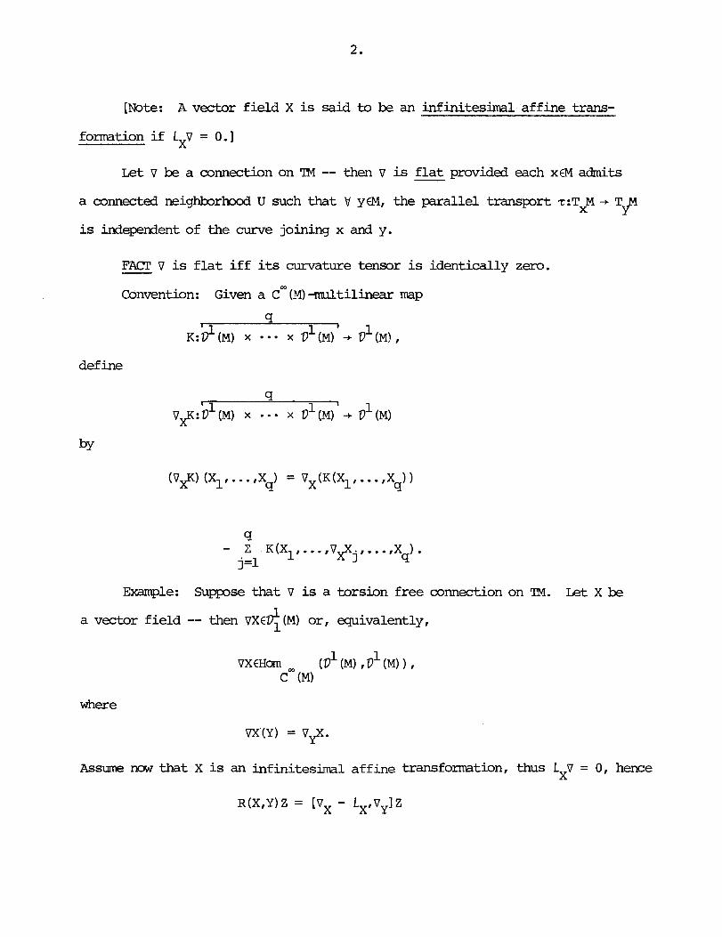
[Note: A vector field X is said to be an infinitesimal affine trans-

formation i f V = 0.1

L e t v be a connection on TM -- then v is f l a t provided each xfM admits

a connected neighborM U such that V y€M, the parallel transport cTXM -+ T M Y

is independent of the curve joining x an3 y.

FAL117 v is f l a t i f f its curvature tensor is identically zero. - Convention: Given a cm (14) -multi l inear map

define

Example: Suppose that V is a torsion free connection on TM. Let X be

a vector field -- then VX€< (MI or, equivalently,

where

VX(Y) = V y X .

Assume now that X is an infinitesimal a f fke transformation, thus L V = 0, hence X

R(X,Y) Z = [Vx - Lx, vy] Z

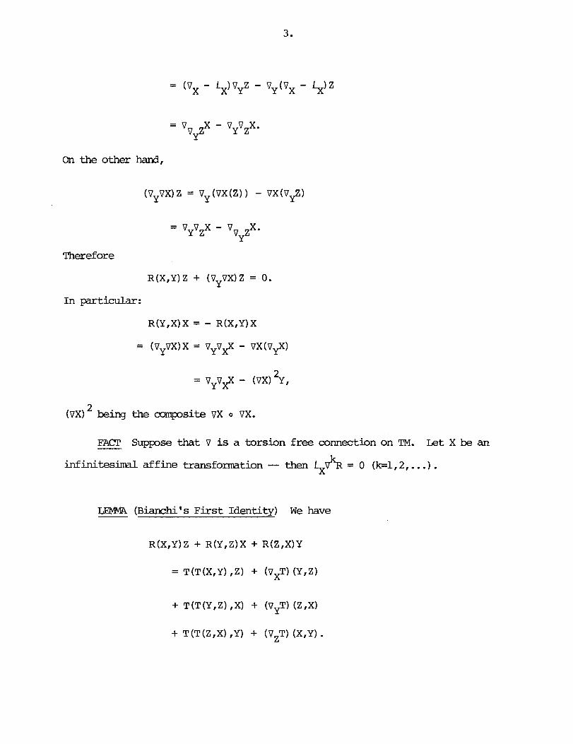
On the other hand,

Therefore

R(X,Y) Z + (VyVX) Z = 0.

In particular :

R(YIX)X = - R(XIY)X

2 (7x1 being the composite VX o VX.

FACT Suppose that V is a torsion free connection on TM. L e t X be an

infinitesimal aff ine transformation -- then ~ ~ d l ( = 0 (k=l , 2 , . . . ) .

UMMA (~ianchi ' s F i r s t I d e n t i t y ) We have

[Note: Consequently, i f V is torsion free, then

- R(VZX,Y) - R(XIVZY)

the bracket standing for a cannutator of operators on vector fields.

[Note: To see where this is caning from, think of R as an element of

LEMMA (Bianchi' s Second Identity) We have

[Note: Consequently, i f V is torsion free, then

Since

there exists a unique derivation

D R(XrY)

:D(M) + (M)

1 which is zero on cm (M) and equals R (X ,Y) on D (M) .

LFM@i ( T h e Ricci I d e n t i t y ) L e t T€$(M) -- then 9

2 2 V TC-tX,Y) - V T(-,Y,X)

where V T ( X t Y )

is the covariant derivative a t the torsion T(X,Y) of V.

[We have

0 Remrk: &t T€$ (M) -- then

So, if V is torsion free, then

Wrking locally, write

a a a i R+ -+ - = R

a

ax ax ax7 jke

thus

Curvature Fonnulas Ass- that V is torsion free.

Bianchi's First Identity:

~ianchi's Second Identity:

One can also write down local

i R j*;L = O*

expressions for the Ricci identity.

Example: Let XCD'(M), say X = ~j 2- -- then V~XCV;(M) and ax j

i i VbVaX - VaVbX

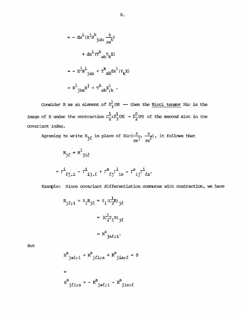
Consider R as an element of 4 (M) -- then the Ricci tensor Ric is the

1 1 0 image of R under the contraction C2 : DJ (M) -r D2 (M) of the second s lo t in the

covariant index.

Agreeing to write R in place of Ric j l

, it follows that

Exarrp?le: Since covariant differentiation ammutes with contraction, we have

But

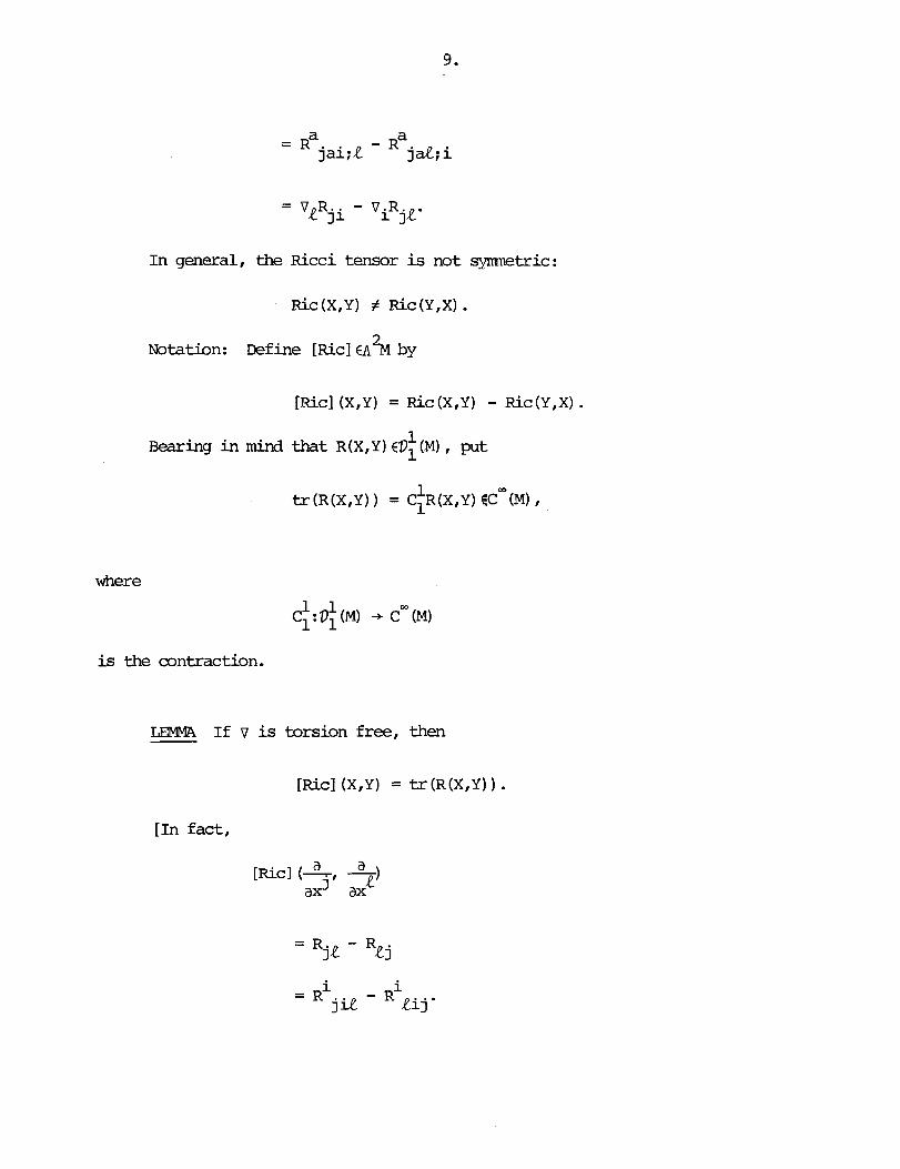
In general, the Ricci tensor is not symnetric:

R i c ( X , Y ) # R i c ( Y , X ) .

Notation: ~ e f ine [Ricl a% by

[Riel (X,Y) = Ric (X,Y) - R i c ( Y , X ) . 1

=ing in mind that R(X,Y) €Dl (M) , put

where

is the contraction.

LEMMA If v is torsion free, then

[Ricl (X,Y) = t r ( R ( X , Y ) . [In fact,

On the other hand,

a i tr(R(-- 5)) = R

axj ' ax ijR

= - i i je i - R R i j

- i I - R j a - R R i j '

Observation: W e have

- i i r i - r i ra - ti, j - j i + i ja ja R i

So, i f 3 a cm function £ of the coordinates such that

Thus, on this chart, Ric is syrtnnetric.

Maintaining the assmnption that V is torsion free, let us globalize

these considerations.

LEWIA Suppose that 4 is a s t r i c t l y positive density of weight 1 such that

V4 = 0 -- then Ric is syrranetric.

[In fact ,

0 = va4 =',a - +'*4

[Note: This can also be read the other way in that the relation

obviously implies tha t V+ = 0.1

By way of notation, put

Then

If now cp is a density of weight r, then

Therefore

Section 10: Semiriemmim -Manifolds Let M be a connected C- manifold

of dimension n.

0 Definition: A semirienannian structure on M is a symnetric tensor gfD2(M)

such tha t V x,

gx:TxM x TxM + - R

is a scalar product.

[Note: A riemannian structure on M is a positive definite semirimimnian

structure. I

Notation: M - is the set of semiriaMnnian structures on M I thus

M = - u O s k s n Ek,n-k '

where Mk - ,n- is the set of scmiriemannian structures on M of signature (k,n-k)

(SO is the set of r iammian structures on M) . Let gfM - -- then one may attach to g its orthonorm1 frame bundle

[Note: Therefore LM(g) is a reduction of LM and the set of reductions

of Dl per the inclusion - 0 (k,n-k) -t - GL (n,R) - is in a one-to-one correspondence

Rappel: IN is either connected or has tsm canrponents.

M is nomrientable i f LM is connected.

M is orientable i f LM has cc~c[ponents.

[Note: I f M is orientable, then the components of Wl are called orientations

and to orient M is to make a clmice of one of them, i n which case M is said to

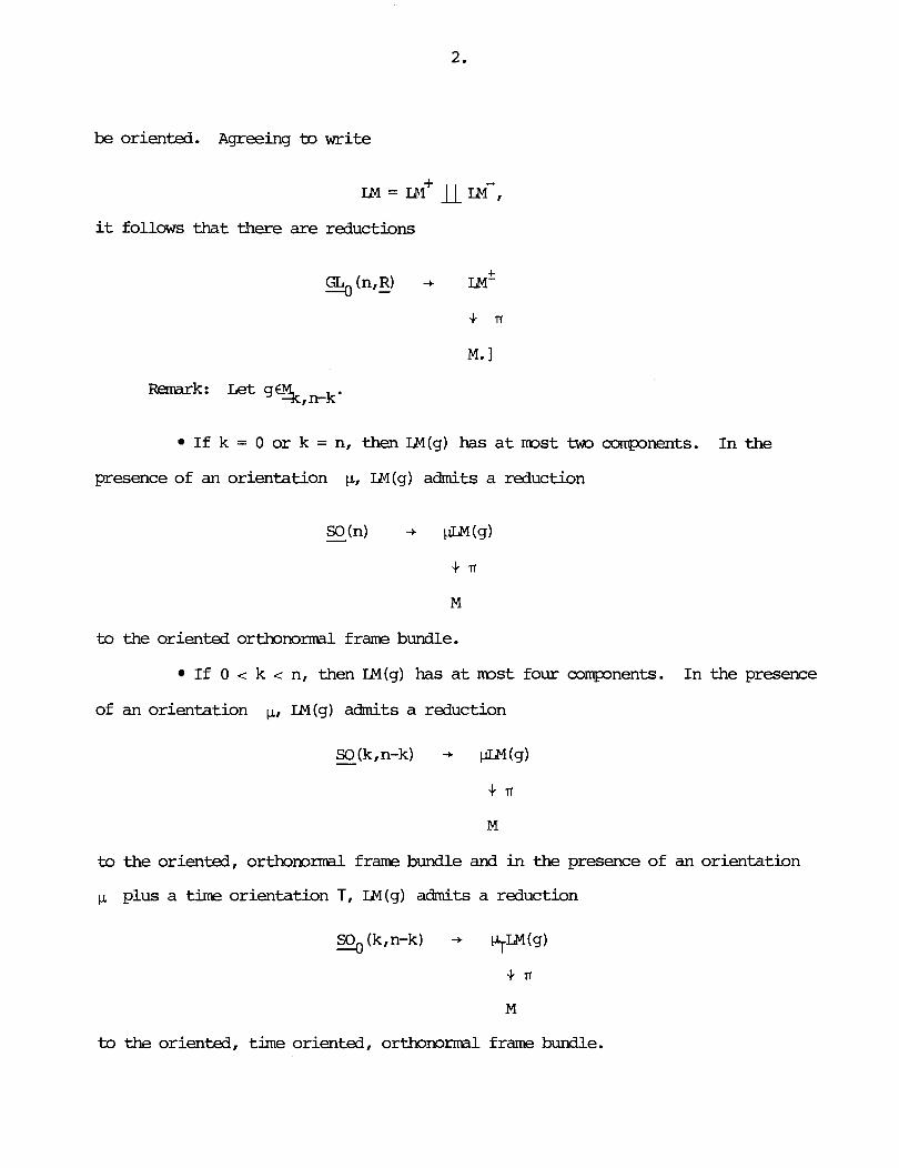
be oriented. Agreeing to write

it follows that there are reductions

Remark: Let g%,n-k*

I f k = 0 o r k = n, then IM(g) has a t mst tm mqmnents. I n the

presence of an orientation p, LM(g) admits a reduction

so(n) -+ W ( g ) - S n

M

to the oriented o r t b n o r m l frame bundle.

I f 0 c k c n, then IM(g) has a t mst four compnents

of an orientation w, IN (g) admits a reduction

In the presence

SO (k, n-k) + U (g) - S lf

M

to the oriented, orthomrmal frame bundle and in the presence of an orientation

p plus a t ime orientation T I IM(g) admits a reduction

SO (k,n-k) -+ v p l ( g ) ---O

S n

M

to the oriented, time oriented, orthonormal frame bundle.

Given g€M, - a connection V on TM is said to be a g-connection i f vg = 0,

1 i.e., if V X,Y,Z€D (M),

Among a l l g-connections, there is exactly one w i t h zero torsion, the metric

connection, its defining property being the relation

FACT Every connection on LM(g) extends uniquely to a connection on LM,

these extensions being precisely the g-connections.

L e t con TM stand for the set of g-connections on TM. g

kmte by I$ (M) the subspace of D; (M) consisting of t b s e Ll such that 4

L e t V ' , Vll €con TM -- then the assignment 9

- 1 1 P1 (M) x (M) x D (M) + cm (M)

(A,X,Y) + A(V$Y - ViY) 1 defines an element of D2 (M)

4 '

[In fact,

L e t VCcon TM -- then Y +~4 (.PI) g, the assignment g

+(M) x +(M) -+ VxY + +(X,Y)

is a g-connection.

[In fact,

= Xg(Y,Z) . I

Scblium: con ?M is an af fine spce with translation group Z$ (M) g.

[The action V-Y = V + Y is free and transitive.]

b 1 Notation: g :V (M) + # (M) is the arrow defined by the rule

b g X(Y) = g(X,Y) .

b -1 It is an i m r p h i s m and one writes gX i n place of (g ) . # Ekample: The gradient grad f of a function fCrn (M) is g (df) . So,

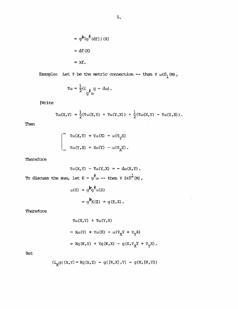
= Xf.

maple: I,& v be the metric connection -- then V w€V1 (M) ,

[ W r i t e

Then

- Vo(X,Y) = Yw(X) - w(v$

- Vw(Y,X) = Xw(Y) - w(VxY) . T h e r e f ore

Vo(X,Y) - Vo(Y,X) = - dw(X,Y) . W 1 To discuss the sum, let K = g w -- then V Z ED (M) ,

b # w(Z) = 9 g ~ ( 2 )

b = g K(Z) = g ( K , Z ) .

Therefore

Vo(X,Y) + Vo(Y,X)

= xw(Y) + Yw(X) - w (VXY + VyX)

But

FACT Fix cp €cm (M) : p O and put 3 = cpg. Let

- v

be the m t r i c connection associated with I Then

1 LEMMA Let v be a g-connection -- then b' XED (M) , the diagram

camutes . [In fact,

b g (VXY) (Z)

-1 2 Notation: g ED (M) is characterized by the cordition 0

g-l (gqr .gb = g (XIY)

Therefore 6'

Kronecker tensor K.

Observation:

[We have

2 2 1 @ g€D2 (M) and the contraction Cl @ g) €Dl (M) is the

Let v be a g-connection -- then vg-' = 0.

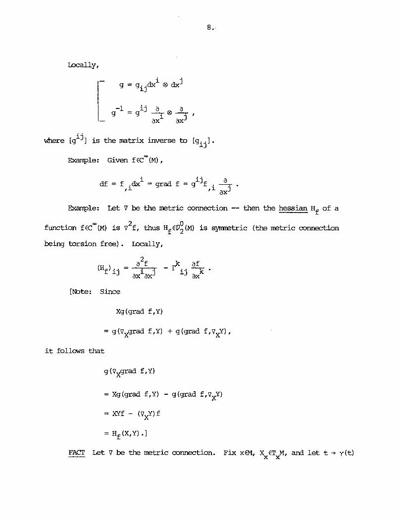
where is the matrix inverse to [g. . I . 13

Example : Given f €Cw (M) ,

Ekample: Let V be the metric connection -- then the hessian Hf of a

2 0 function ~ C C * ( M ) is v f , thus HfhV2(M) is symetric (the metric connection

being torsion free) . Ir>cally,

= g ( V X 4 r a d f ,Y) + g (grad f , vXY) ,

it follows that

= Xg(grad f , Y ) - g(grad f,VXY)

= XYF - (VXY)f

= Hf(X,Y) - 1

FACT Let V be the metric connection. Fix x€M, X x C T 2 , and let t + y ( t )

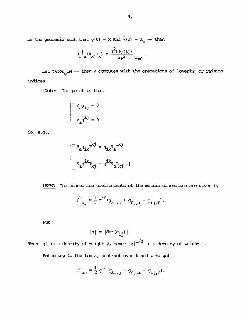
be the geodesic such that y(0) = x and j ( 0 ) = Xx -- then

Let VCcon TM -- then v camnutes with the operations of lowering or raising 4

indices.

[Note: The point is that

~~j = g v I- vagik

~~j i k a

IDMA The connection mefficients of the metric connection are given by

Put

Then 1 g 1 is a density of weight 2, hence 1 g is a density of weight 1.

Returning to the lama, contract over k and i to get

But

Theref ore

= (det g) -1 adet g

ax j

1 Exarrq?le: L e t v be the m t r i c connection. Suppose that XED (M) -- then

V X C ~ (M) and, by definition, the divergence div X of X is

1 div X = ClvX ( = tr vX) . mcally ,

or still,

div x =

[Note: The laplacian Af of f € c m (M) is the divergence of its gradient:

or still,

0 = gE21 (Hf,Hf) + g(grad f , grad A f )

Let V be a connection on TM -- then

+ Ric(grad f , grad f) .

Now take for V the metric connection:

[Note: Write

Then

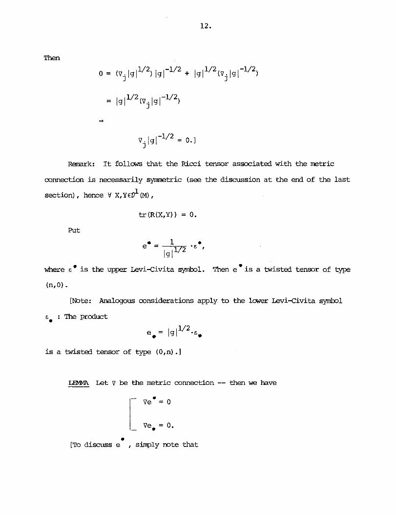
Remrk: It follows that the Ricci tensor associated with the metric

connection is necessarily qmnetric (see the discussion a t the end of the l a s t

section) , hence \I X,Y& (M) ,

where E' is the upper Levi-Civita symbol. Then e ' is a twisted tensor of type

(n,O) . [Note: Analogous considerations apply to the lower Levi-Civita symbol

&. : The product

e*= Ig

is a twisted tensor of type (0,n)

LENMA Let V be the metric connection -- then we have

vem= o

0

[To discuss e , simply mte that

Let V be a connection on TM -- then the assignment

and

14.

Let V be the metric connection:

RijM + RMj + Riejk = 0

RijU = Qij .

[Note: Recall too that

Rijl&;m + Rijh;k + Rijmk;L =

Example: The Kretschmam curvature invariant kR is, by definition,

THM)REN Let V be the mt r i c connection. Fix a p i n t xOEM and l e t

1 n x ,..., x be normal coordinates a t x -- then 0

Let V be a torsion free connection on TM -- then

(Lxg) (YIZ) = (Vxg) (YIZ)

+ g(V9,Z) + g(Y,VzX).

In particular, when V is the metric connection,

(Lxg) (YIZ) = g(VyX,Z) + g(Y,VzX).

Observation: Let v be the metric connection -- then

= V$X(Y.Z) + V&(Z,Y).

[Note: Lacally,

1 1 b (v3lb = L ~ ( ~ ~~g + 7 d~ 1.

Let XCD' (M) -- then X is said to be an infinitesimal isometry if LXg = 0.

FACT An infinitesimal isometry is necessarily an infiniteshl affine

transformation.

Fram the definitions,

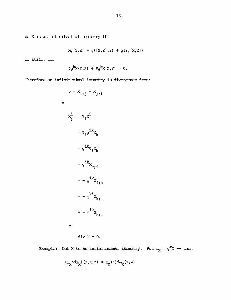
so X is an inf in i tes iml ismetry iff

Therefore an infinitesimal isometry is divergence free:

*

div X = 0.

Example: L e t X be an infinitesimal iscmetry. Put y( = g h -- then

Analogously

Therefore

Assume now that

0ydi.k = 0.

Let 4 = g(X,X) ( = %(X)) -- then

C

It thus follows £ran the Poincare l m that locally,

y, = g(X,X)df (3 f) .

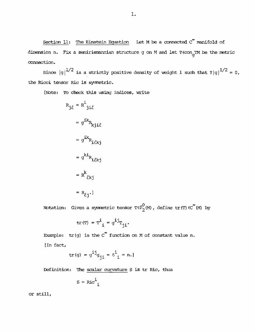
Section 11 : The Einstein Equation Let M be a connected cm manifold of

dimension n. Fix a s e m i r i d a n structure g on M and let vccon TM be the metric 5.l

connection.

1/2 Since 1 g /Ii2 is a s t r i c t l y p s i t i v e density of weight 1 such that V / g ( = 0,

the Ricci tensor Ric is symnetric.

[Note: To check th i s using indices, write

0 ~o ta t ion : Given a symnetric tensor T C D ~ (M) , define tr (T) C C ~ ( M ) by

tr (T) = Ti - i j i - T j i *

Example : tr (g) is the cm function on M of constant value n.

[In fact,

i j t r ( g ) = g gji = €ii = n.] i

Definition: The scalar curvature S is tr Ric, thus

or still,

s = g %j i j k

j k = R jk'

Notation: Write

ab va = g vb.

LEMMA (The Elmhwntal Identity) W e have

1 0% = Y k S .

[To begin w i t h

O = Rijlce;m + RijhPk + Rij&;L

= V R m i j k L + VkRijh + VLRij*.

T h e r e f o r e

jL mi 0 = 9 9 (P,Rijlce + VkRijh + VLRij*) .

Now examine each term i n succession.

j R m i (1) g g VmRijke

j R im, = g g ijw

j l 5 = 9 v i j M

i j% = v 4 iju

= Pi.j".,eij

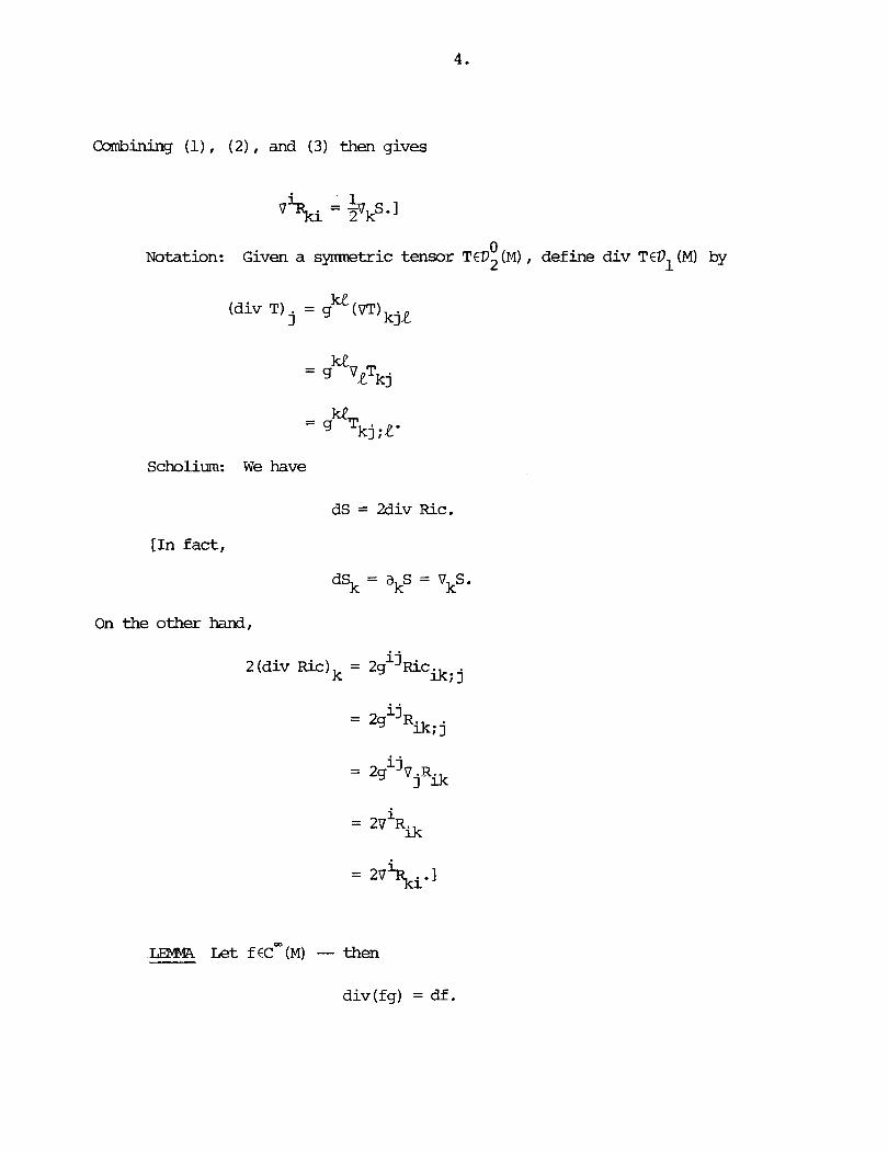
0 Notation: G i v e n a synmetric tensor TED2 (M) , define div T€Dl (M) by

Scholium: W e have

dS = 2div Ric.

[In fact,

dSk = akS = VkS.

On the other hand,

Let f C C ~ O (M) -- then

div (fg) = df .

[For

div Ric = div(+g)

On the other hand,

Therefore

Definition: The Einstein tensor Ein is the combination

1 Ein = F t k - q Sg.

0 So, EinED2 (M) is symmetric and one has

1 div Ein = div Ric - .Z. div(Sg)

1 = div Ric - -2- dS

= 0.

In addition,

*

tr Ein =

Therefore

[Note: When n = 4,

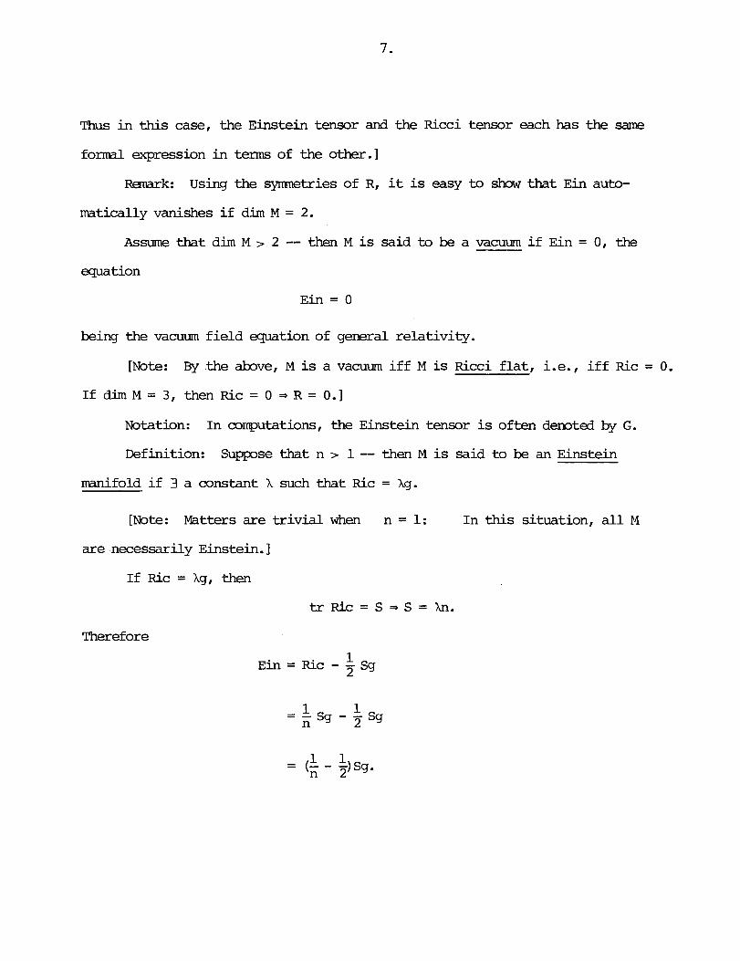
Thus in this case, the Einstein tensor and the Ricci tensor each has the same

formal expression in terms of the other.]

Remark: Using the symnetries of R, it is easy to &ow that Ein auto-

matically vanishes i f dim M = 2.

Assume that dim M > 2 -- then M is said to be a vacuum i f Ein = 0, the

equation

E i n = 0

being the vacuum field equation of gensral relativity.

[Note: By the above, M is a vacvum i f f M is Ricci f l a t , i.e., i f f Ric = 0.

If dim M = 3, then Ric = 0 =, R = 0.1

Notation: In computations, the in stein tensor is often demted by G.

Definition: Suppose that n > 1-- then M is said t o be an Einstein

manifold i f 3 a constant X such that Ric = X g .

[Note: Matters are t r iv ia l when n = 1: In this situation, a l l M

are necessarily Einstein. I

If Ric = kg, then

Therefore

Section 12 : Deccrmposit ion T h e o r y Let V be an n-dimensional real vector

space. Suppose that A:V + V is a linear t r a n s f o r m a t i o n -- then

where

and

Therefore

Notation:

Ham(V,V) = Ker ( t r ) @ - R I .

R is the set of mltilinear maps

R : V x V x V x V + R -

such t h a t

m l e : Let M be a connected cW manifold of dimension n. Fix g€M - and

let V be the metric connection -- then a t each x€M, the tensor

(W, 2 ,X,Y) -+ g (R(X,Y) Z ,W)

induces a multilinear roap

satisfying (a) - (d ) .

1 2 2 LEbNA R is a rml vector space of dimension n (n -1).

[Note : Therefore

n = l * d i m R = O ;

n = 2 = + d i m R = l ;

n = 3 = d i m R = 6 ;

n = 4 =, dim R = 20.1

Definition: L e t P,Q:V x V -t - R be symnetric bilinear forms -- then the

curvature product of P,Q is the tenmr P xc Q of type (0,4) defined by

P Xc Q(X1tX2tX3tX4)

- p(x,,x4)Q(X2.X3) - P(X2fx3)Q(XlfX4).

Obviously,

P x c Q = Q x c P

and it is not diff icul t to check that

P Xc QER.

Now f ix g€M - -- then the prescription

r: This is themap - 0 r : R -+ Sym V2

defined by

m e EEB (V) is orthonoml.

[Note: rR is independent of the choice of E. 1

0 Notation: Given TfSym V2, put

W e shall then agree to write sR i n place of tr (rR) , thus

= ~ r (E E ) + - - - + ~ r (E E ) . S~ 1 R 1'1 n R n ' n

Remark: Let M be a connected cm manifold of dimension n. Fix g€M - and

l e t V be the metric connection -- then a t each x€M,

s = S (x) . I- Rx

[By definition,

where

Ricx(X,Y) = t r ( Z -t R(Z,X)Y) . So, if {El, ..., En) is an ortbmrmal basis for TXM per gx, then

And

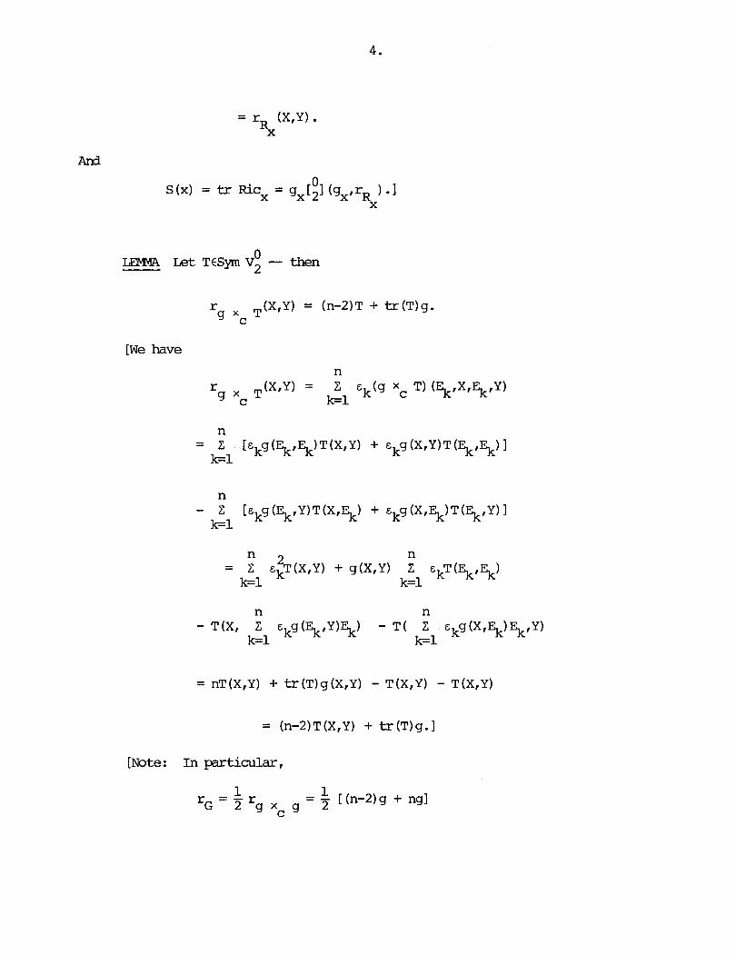
LEWA ~t ~ t s y m V: - then

r (X,Y) = (n-2)T + t r ( T ) g . 9 XC T

[We have

= (n-2)T(X,Y) + t r (T Ig .1

[Note: In p a r t i c u l a r ,

- 1 - - r 1 = - [ (n-2)g + ng]

IG 2 g x c g 2

Elxample: S u p p s e that n = 2 -- then dim R = 1, hence V RCR, 3 CR€R: -

R = CRG

Therefore

Assume that n > 2 and let R€R -- then

where, by definition,

or still,

o Write Symo V2 for the kernel of

0 tr:Sym V2 -+ - R.

Example: V RER,

1 S - R - -glE Sym V 0

n-2 R n o 2'

Write C for the kernel of

r : R -t Sym V 0

0 2'

Example: V RER, CEC.

[In fact,

immB There is a direct sum decomposition

0 R = R ( g x - g) CHSym V x g @ C . C 0 2 c

[Note: MDre is true in that the deccenposition is or'daogona

Remark: If n = 3, then

But 1 2 2 dim R = - 3 (3 -1) = 6. 1 2

Consequently, C is t r ivial , thus i n this case

Definition: The elements of C are called the Weyl tensors.

L e t M be a connected cW manifold of dimension n. Fix g€M - and l e t V

the metric connection -- then the preceding considerations can be globalized in

the obvious way, the key new ingredient being the Weyl tensor (n > 3) :

I be the metric connection associated with I .

Then

N

C = (PC.

1 [Note: Therefore the Weyl tensorI when viewed as an element of D3(M),

is a conformal invariant. I

Section 13: Bundle Valued Forms Let M be a connected cm manifold of

dimension n. Suppose that E -t M is a vector bundle -- then the sections of

E ~3 A~T*M are the p-forms on M with values in E.

Notation: Put

AP (M; E) = sec (E B APT*M) . [Note: When p = 0,

0 A (M;E) = sec(E) . I

Structurally,

0 A ~ ( M ; E ) = A (M;E) (i3 A ~ M ,

cm (MI

thus the elements of ~'(M;E) are the c-(M) -multilinear antisymnetric maps

Remark: If E is a t r iv ia l vector bundle with fiber V, then -

AP(M;E) is

the space of pforms on M with values in V and is denoted by A'(M;v) . Example: Let

be a principal bundle w i t h structure group G (which we shall take to be a L i e

group). Let p be a representation of G on a real f in i te dimensional vector

space V -- then a pform

is said to be of type p i f

-1 (Ro)*a= p(o ) a V aEG.

Write

for the space of pforms on P of type p and l e t E be the vector bundle

Then thexe is a canonical one-im-one correspondence

Suppose that E + M is a vector bundle. Let V be a connection on E -- then V gives r i se to an R - l i n e a r - map

0 1 V:A (M;E) -t A (M;E)

such that

viz . v s (X) = v p

Conversely, every - R - l i n e a r map

determines a connection on E. Thus l e t X C D ~ (M) -- then X induces a c-(M) -linear

rmp w A -+ C ) , hence there is an arrow X

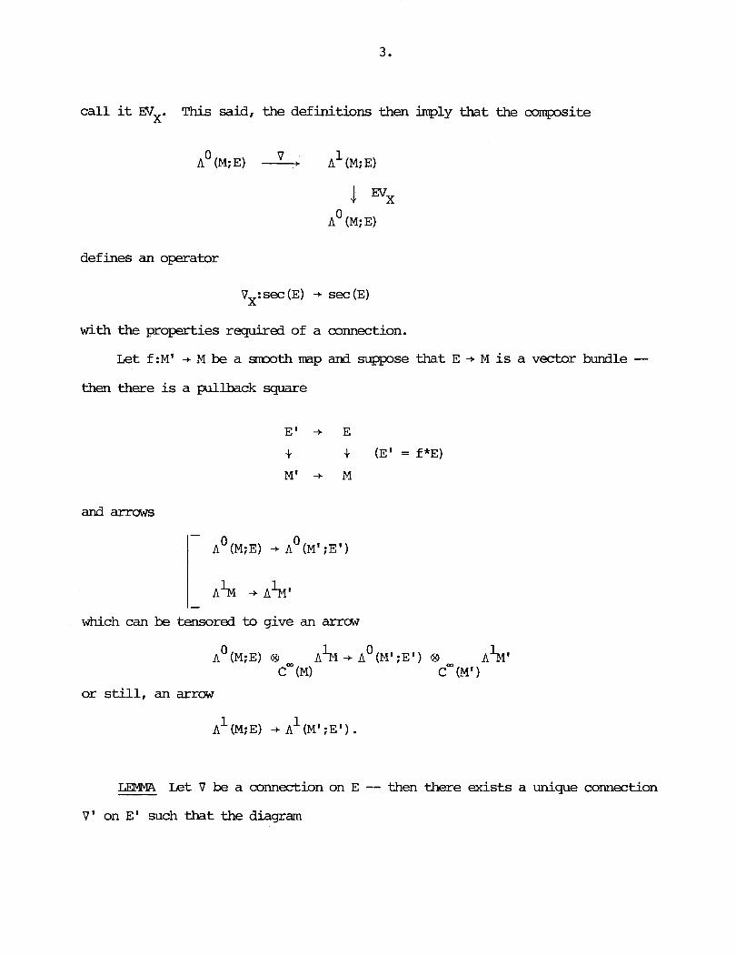
call it EVx. This said, the definitions then inply that the mmpsite

defines an operator

Vx:sec (E) - sec (E)

with the properties required of a connection.

Let f:M1 -t M be a mth map and suppose that E -t M is a vector bundle -- then there is a pullback square

and arrows

which can be tensored to give an arruw

Let V be a connection on E -- then there exists a unique connection

V ' on E' such that the diagram

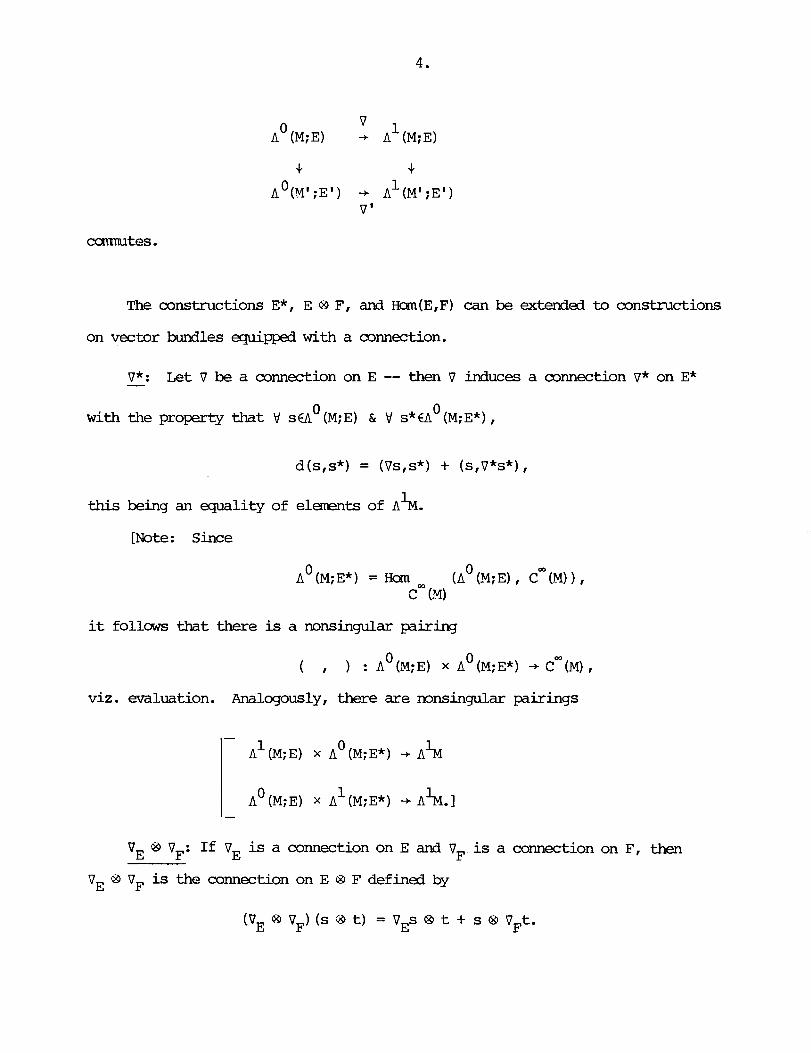
The constructions E*, E €9 FI and Hom(E,F) can be exterded to constructions

on vector bundles equipped w i t h a connection.

V*: Let V be a connection on E -- then V induces a connection V* on E* -

0 0 with the property that V s€.A (M;E) & V s* €A (M;E*) ,

this being an equality of elements of A%.

[Note: Since

0 A (M;E*) = Hom

0 (A (M;E) , cm (M) ) ,

cW (MI

it follows that there is a nonsingular pairing

viz. evaluation.

0 0 ( , ) : A (M;E) x A (M;E*) +c- (M) ,

Analogously, there are nonsingular pairings

VE PO OF: If V is a connection on E and VF is a connection on F, then E

vE @ vF is the connection on E @ F defined by

1 [Note: The tensor products on the r igh t are elesnents of A (M;E @ F ) . For

' H ~ ~ ( E , F ) : L e t VE be a connection on E and let VF be a connection on F --

Men the @ r ( V E , V F ) induces a connection V Hm(E,F) on Hom (E ,F) with the property

= (d)IvEs) + (vHm(E,F) +Is) I

1 this being an equality of elements of A (M;F) .

[Note: F i r s t , there is a nonsingular pairing

Second, there is a mnsingular pairing

Rg0aTk: U n d e r the identification E t-t E**, we have V * V**, and under

the identification E* 8 F ++ Hom(E,F), we have BE, 8 F - 8 Hm(E,F) '

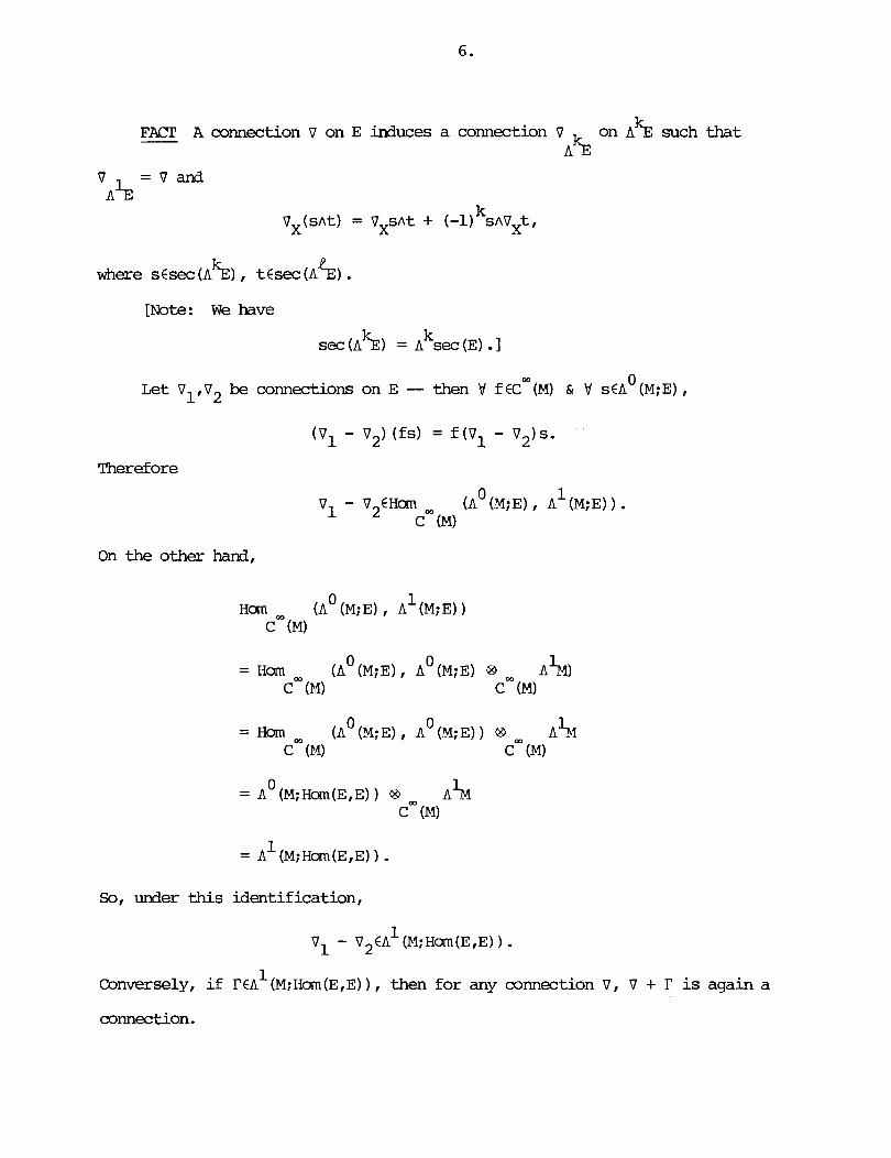
FNX A connection v on E induces a connection V on A% such that h

V = V and A%

k vx(snt) = vxsnt + (-1) snvl(t,

where s~sec (A%) , t~sec (A%) . [Note: We have

sec (A%) = Aksec (E) . I

0 Let V1,V2 be connections on E -- then V f€Cm(~) & \I sfA (M;E),

(vl - V2) (fs) = f(V1 - V2)s. Therefore

V1 - V2€Hm (A 0 (M; E) , A 1 (M;E) ) . Cm (MI

On the other hand,

= Ham 0 0 (A (M;E) , A (M;E) PD Ah)

cm (M) cm (M)

So, under this identification,

Conversely, if !?€AL (M; H m (E ,E) ) , then for any connection V , V + I' is again a

connection.

Let con E stand for the set of connections on E.

1 Scblium: con E is an affine space with translation group A (M;Ham(E,E)).

[The action V-r = V + I' is free and

Reality Check Take E = TlvI -- then

A'(M;H~~(TM,TM)

transitive. 1

P- Suppose that E = El 63 E2 -- then there are canonical arrows

I- con E + con E2

viz .

Let E -t M, F -+ M be vector bundles -- then there is a CW(M) -bilinear product

which is characterized by the condition

( s @ a ) A ( t @ $ ) = ( s @ t ) @ (aA$).

[Note: W e have

and

0 0 A (M; E B F) = A (M; E) C3 0

A (M;F) . C* (MI

0 Therefore s 69 t is an elanent of A (M;E @ F) .I

Example: Take F = E = M x - R, the t r iv ia l l ine bundle -- then

Since

and E 8 E = E, it follows that

sAa = s 63 a

in AP(M;E) . Suppose that E -+ M is a vector bundle. Given vfcon E, l e t

be the - R-linear operator defined by the rule

[Note: Recall that vs€A1 (M;E) . Now view a€AP!!l as an element of AP(M; E ) --

~t is easy to check that dv = v h e n p = 0.

= dv(s 9 a)ng + (-llP(s 8 a)~dp.I

[Mte: This, of course, is an equality of eletwts in A*" (M: E) .I

P Eample: Take E = 6, so Y p, A (M:e) = APM. Consider the m p

I - f --+ df.

v Then d is a connection V and d is the usual exterior differentiation.

FACT Let E -+ M, F + M be vector bundles -- then there is an R-linear map -

Suppose that E is a vector bundle and let V be a connection on E -- then

there is a sequence

which, in general, is not a c a p l e u since it need not be t rue that dv o v = 0

v (likewise for dV 0 d ) . v 0 2 Put F' = dv 0 V -- then F is a map from A (M;E) to A (M;E) ard is

C" (M) -linear. Indeed,

V = d V ( s 69 df) + d ( ~ V S )

= f (dV 0 V ( S ) ) .

On the other hand,

2 = A ( M ; H ~ ~ ( E , E ) ) .

D e f i n i t i o n : The curvature of V is

V 2 F EA ( M ; H ~ ( E , E) . L e t s @ a€AP(M;E) -- then

v = F ( s ) ~ a .

Therefore

0 V I dv 2 dV 0 -t A (M;E) -t A (M;E) -+ A (P4;E) -t

v is a complex provided F = 0.

LI3WR W e have

V v d F = 0 ,

v where d is associated w i t h Vm (E, . 2 0

[ V + € A (M;Hom(E,E)) & V SEA (M;E),

3 this being an equality of elanents of A (M:E). Take 4 = -- then

v v v v (d F ,s) = d (F ,s) - (FVfVS)

= dV 0 (dv o Vs) - (dV o dV) 0 Vs

R(X.Y) = Vx 0 Vy - Vy 0 Vx - * [XIYI Then

0 0 R(XfY) :A (M;E) -+ A (M;E)

mme is also an a r m ev :A% -+ c~(M) which can be tensored over c-(M) XIY

0 w i t h A (M; Ham(E,E) ) to give an arrow

Put

F' = R ( X r Y ) . x r y

Define L~ on A ~ ( M ; E ) (p > 0) by

r X ( s €3 a ) = s O L a. X

0 [Note: Take L~ = 0 on A (M;E) . I

1 0 LEMMA Let X,YEV (M) -- then V SEA (M;E) ,

Reality Check Take E = 6 -- then d2 = 0 and Y f C C ~ ( P O ,

= 0.

Remark: The lerrnrra is merely a r e s t a tma t of the fact that

Rappel: In the exterior algebra A*M,

l\ilotivated by this, given vccon E, put

thus

= t x V s = v s (X) = Vxs.l

FACT We have

Specialize now to the vector bundle

Then the elgnents of

are the cW (M) -multilinear antisymnetric maps

[Note: B e a r in mind that

A 1 ; M ) = z$ (M) . I 9

Rmark: Working locally, each aCAk (M:TP(M) ) defines a k-form 9

these being the cc~nponents of a.

Let V be a connection on 'IM -- then V induces a connection on (N) , which q

again will be denoted by V. Accordingly, there is an - R - l i n e a r operator

with the property that

[Note: Here,

@ p(xO(k+l) r-**fXO(k+l))

0 Example: Take p = q = 0 -- then DO (M) = c~(M) ard

nk (M;c" (MI ) = A%.

In th is situation, dv = d, hence is the same for all V.

Example: -t TcD~; (MI -- then

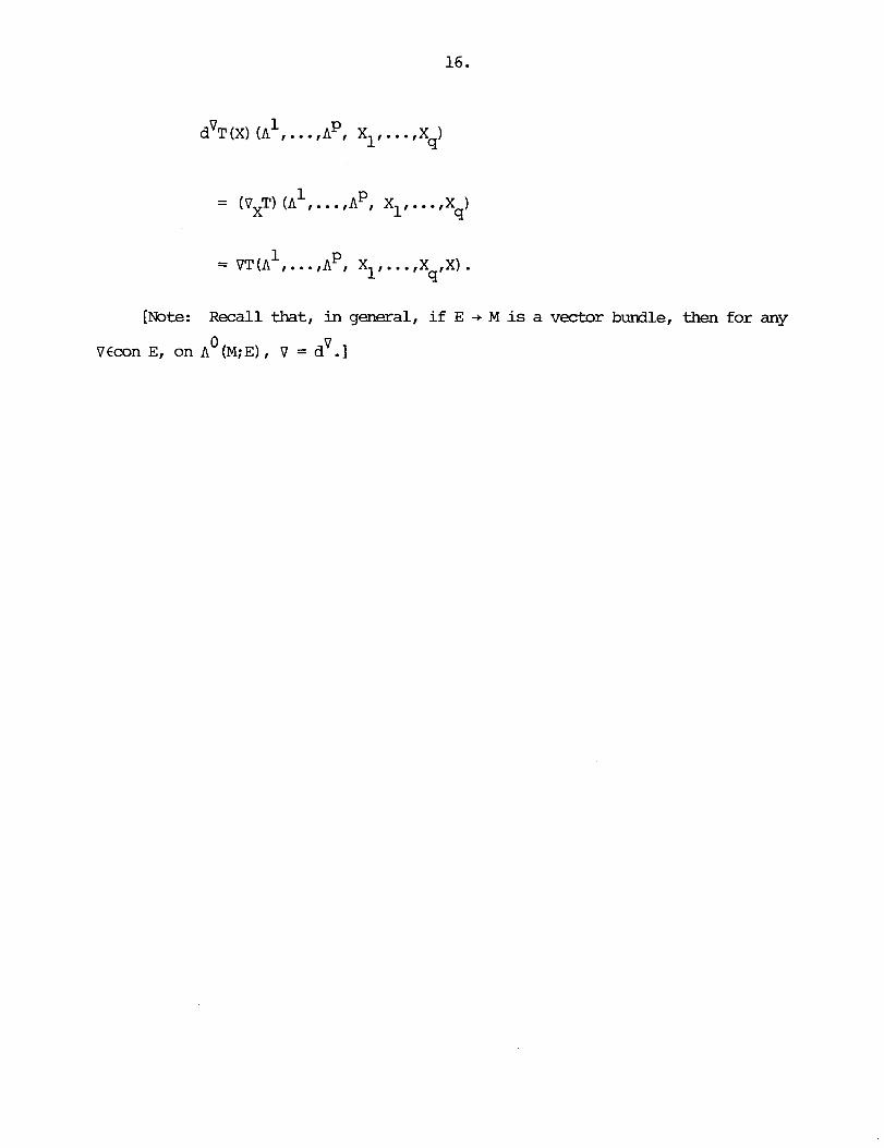
[Note: Recall that, in general, i f E -+ M is a vector burdle, then for any

0 v QEcon El on A (M;E), V = d .I

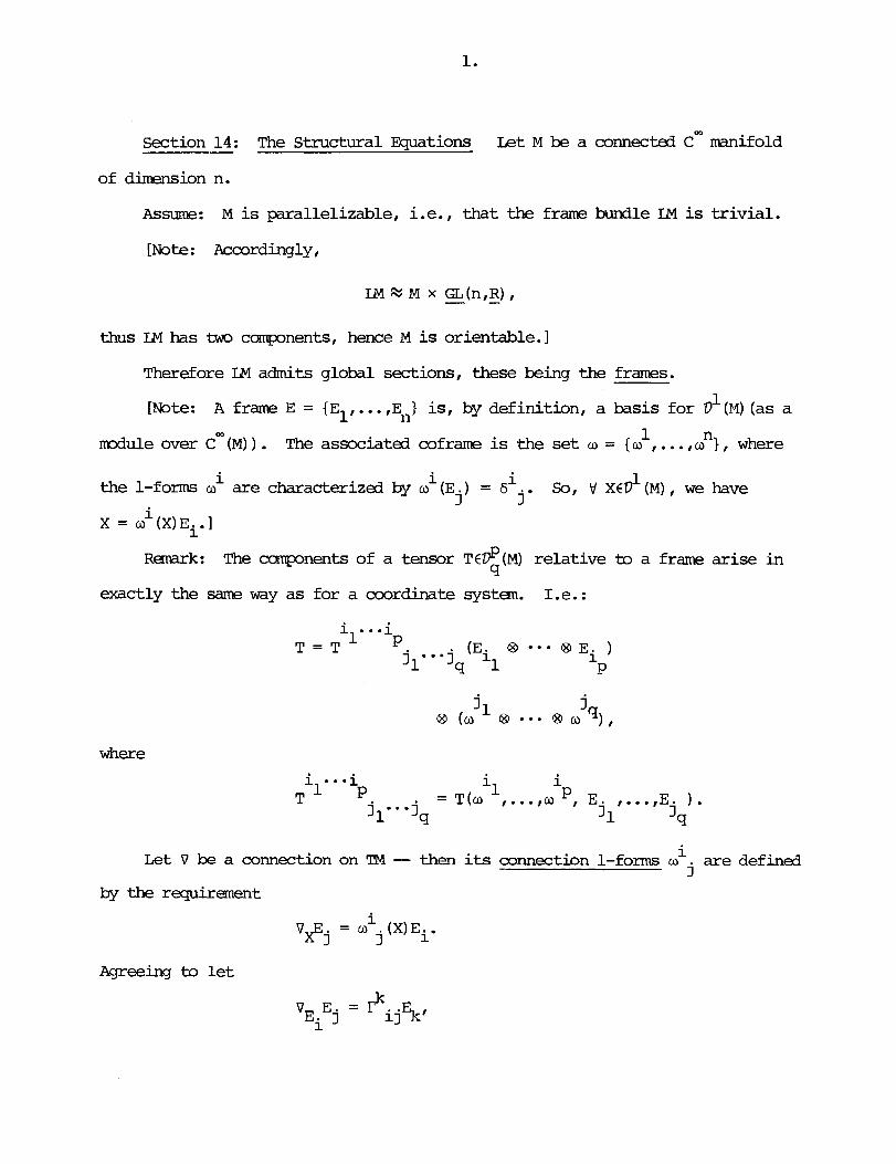
Section 14: The Structural Equations Let M be a connected cW manifold

of dimension n.

Assume: M is parallelizable, i.e., that the frame bundle LM is trivial.

[Note : Accordingly,

thus L&l has tm components, hence M is orientable.]

Therefore LM admits

[Note: A frame E =

d u l e over coo (MI ) . The

global sections, these being the £rams.

1 E l . . . , E l is, by definition, a basis for D (M) (as a

1 associated coframe is the set w = {a , . . . , $1, where

the 1-£0- 2 are characterized by mi (E . ) = gi 1 j

So, t! XED (M), we have 7

Remark: The canpnents of a tensor TE@(M) relative to a frame arise i n 'I

exactly the same way as for a coordinate system. 1.e.:

where

i Let V be a connection on TM -- then its connection 1-forms w are defined j

by the r e q u i r m t

Agreeing to l e t

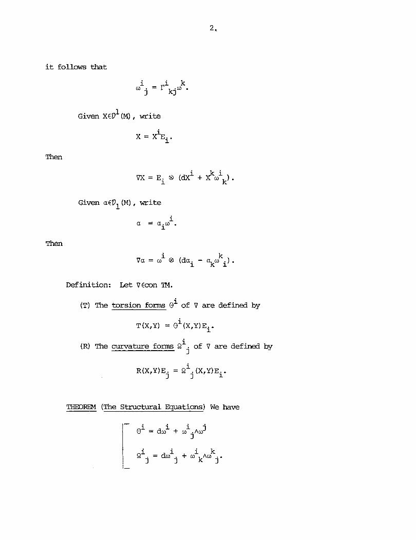
it follows that

1 Given X€Z> (M) , wri te

Then

i - Va = w QD (da

k i - % w i ) .

Definition: L e t V€con TM.

(T) The torsion forms oi of V are defined by

i T(X,Y) = 0 (X,Y)Ei.

(R) The curvature forms 8i of V are defined by j

THM)m4 (The S t r u c t u r a l Equations) W e have

[Consider the f i r s t relation. Thus

j i + {a' (Y) oij (X) - o (X) o . (Y) }Ei 3

Consider the second relation. Thus

i i = {& (Y) - yoi. (X) - o ([X,Y]) }Ei J j

Remark: If V is torsion free, then

i i j do = - a jAW

[Note: Put

Then in the presence of zero torsion,

FACT Suppose that V is torsion free -- then V a € d p ~ ,

Write

Then the ci are the objects of anholonomity. j k

[mte: Their transformation behavior is nontensorial.]

Observation: W e have

- i - - jkEi.

There is an expansion

There is an expansion

[Note: By definition,

Then

The Ric. ( j = 1,. ..,n) are called the Ricci l-forms, Obviously, 3

but, i n general, Rji # Rij.

Section 15 : Transition Formalities Let M be a connected cW manifold of

dimension n.

Rappel: There is a one-to-one correspondence

between the connections l? on the frame bundle

GL(n,E) + ~4 - 4- l-l

M

and the connections v on the tangent bundle

Assume now that M is parallelizable. Fix a frame E = {E ..., En} and let 1'

s:M + LM be the section thereby determined, thus V xCM,

is a basis for TxM.

FACT. Fix x€M and let cx:~" - + TxM be the norsingular linear transformation

(al,. . . ,an) + a E + 1 ilx + "nEn/x*

1 Suppose that X,YEV (MI -- then

i + (XY )(x)Eilx.

1 The correspondence l? t. + s * ~ identifies con IM with .A (#;gL(n.g) - 1.

1 And each V €con TM gives rise to an elenent %€A (M: - gl (n, g) ) , viz .

i 0 = [a j l . v

0 =s*y. vr

[By definition,

On the other hand,

Here

and

But

*

Therefore

In fact,

Definition: A gauge tsansfomtion is a cm map

Notation: - GAU is the set of gauge transformations.

With respect ~ pintwise operations, - GAU is a group and there is a right

action

where

Let VEcon TM - then under a change of frame

the matr ix

[Note: The products are matrix products aM3 dg is the entrywise exterior

derivative of g:M + GL(n,R) .I - -

Remark: The transformation property of !J is simpler, viz. v

-1 R v + g Rvg ( g F E ) ) .

[Invoke the lama and observe that

-1 dl(dg) = - dg .I

In matrix notation, the relation

i V 3 j = w (XI Ei

j

can be written

So, V gEGAU, -

Let v be a connection on TM and consider the - R - l i n e a r operator

Then V ~ € A ~ ( M ; @ ( M ) ) , one has 9

In what follows, use matrix mtation.

Example:

(1) Take p = 1, q = 0 -- then

( 2 ) Take p = 1, q = 1 -- then

TtE oic*% are the components of an el-t

1 Explicated: V XED (MI ,

Analogously, the

are the conpnents of an el-t

1 1 Example: The mi. ~3% are not the compnents of an elenent o CA (M;T1(M) ) . 3 V

Replacing E by E0g changes T~ to j

But this tensor transformation rule is laot satisfied by o since v

o V + g-lovg + didg. 1

v d a: W e have -

dvw = do + w Ao v

v d Ov: W e have

= d (dw + a$w) + ovA (do + ovAo)

= doVAo - w Ado + o Ado + o g A r n V h o v v

dVnv: W e have

= dw Aw - w Ado + o Ad v V v v v v v

Remark: The symbol QV has two meanings, namely as an element of

Of course, if $2 is viewed in the second sense, viz. as a map v

then, u p n taking cmpnents, QV reappears in the first sense as a matrix,

viz. v X,Y&M) ,

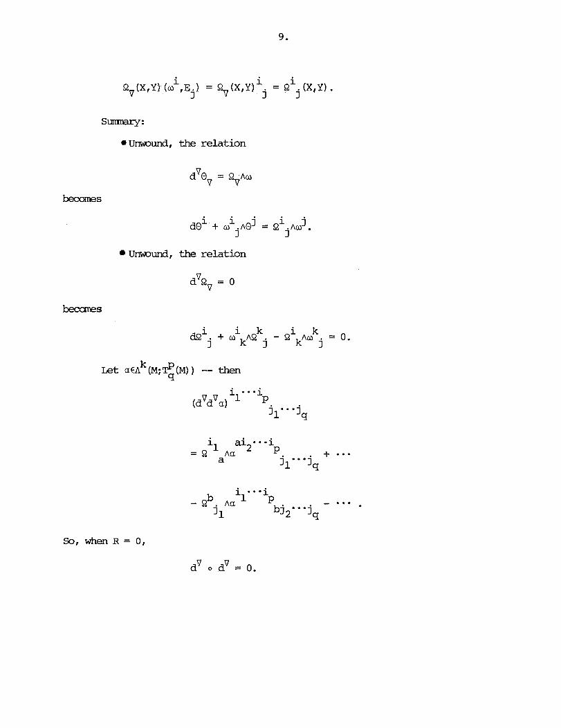
Sumnary:

U m u n d , the relation

U m u n d , the relation

becomes

Let aQlk (M; % (M) ) -- then

So, when R = 0,

dV 0 dV = 0.

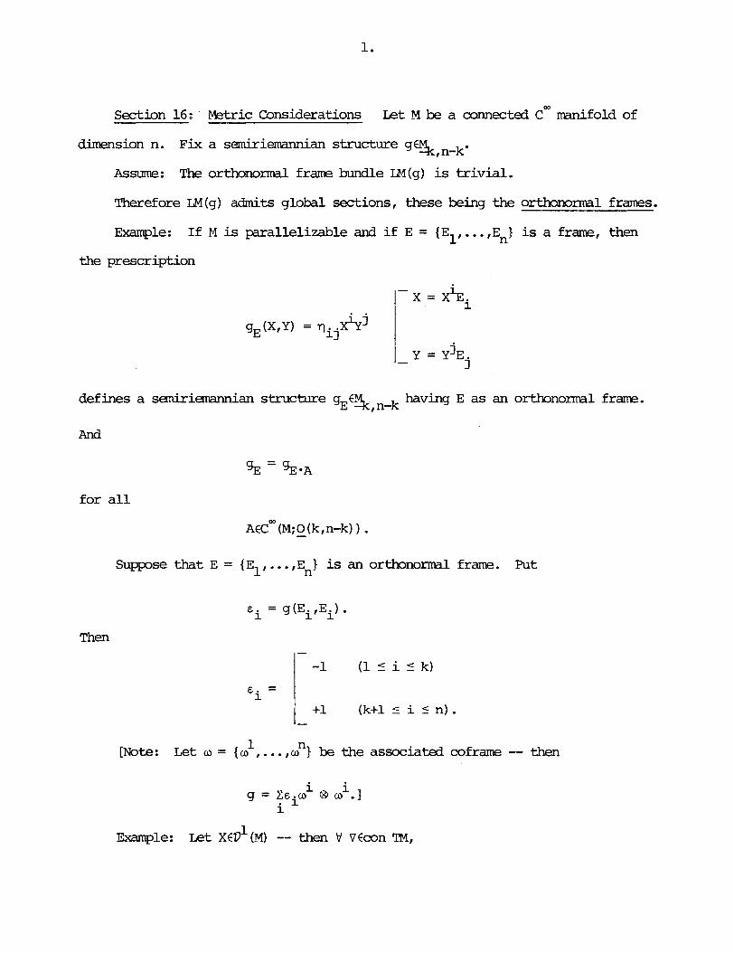
Section 16: Metric Considerations L e t M be a connected cm manifold of

dimension n. Fix a sanirierrardan structure gF% , n-k'

Assume: The orthonormal frame bundle Ud(g) is t r iv ia l .

Therefore LM(g) admits global sections, these being the orthonormal frames.

Example: If M is parallelizable and i f E = {E,, ..., E_) is a frame, then

the prescription

defines a sariximamian structure gEC$,n-k having E as an ortbnormal frame.

And

for a l l

Suppose that E = {El, ..., E } is an orthonormal frame. Put n

E = g ( E E ) . i if i

Then

n [Note: L e t o = 12 ,..., a } be the associated mframe -- then

Example: L e t XED' (M) -- then Q VFmn IM,

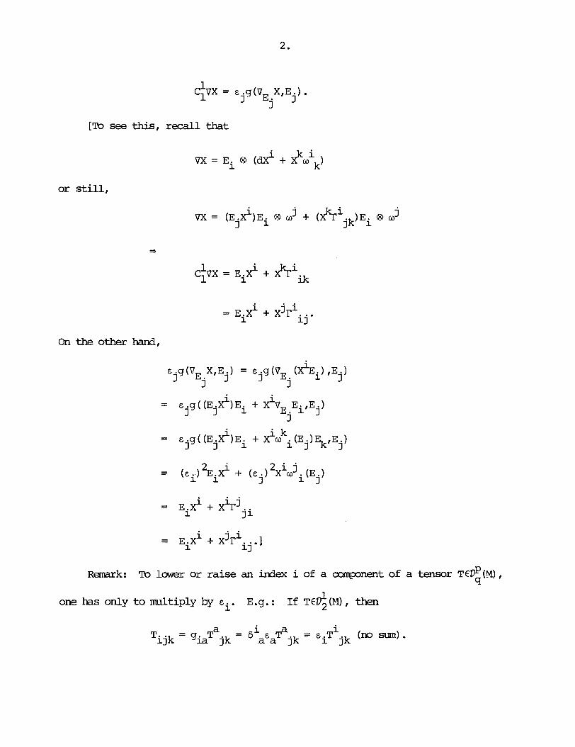
[To see this, recall that

or still,

On the other hand,

ema ark: To lower or raise an index i of a component of a tensor TE$(M), q

one has only to multiply by ci. E . g . : If T€$ (M) , then

Fix VEcon TM. g

UNMA We have

i j = & . L O (X) + e . o . ( X ) (no sum).]

1 j I 1

[Note: If E = (El, ..., E ) is an arbitrary frame, then n

In particular:

LlW4A We have

[In fact,

2 i i k = ( & . & . ) [dm +okAO .I =s? I

11 j I j '

In particular:

i B i = o .

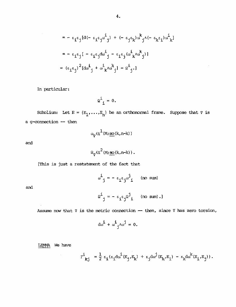
Scholium: L e t E = (El, ..., En} be an orthonorm1 frame. Suppose that V is

a g-connection -- then 1

ov €A (M; - so (k, n-k)

and

2 Q,€A (M;so(k,n-k)) - .

[This is jus t a restatement of the fac t that

i - 0 - - j

j (no s m ) E . E .o 1 1 i

and

Assume now that V is the metric connection -- then, since V has zero torsion,

l2mn W e have

1 i j k f = - . . ( C . ~ ~ ( E ~ , % ) + E . ~ u ( % , E ~ ) - E ~ ~ ~ ( E ~ , E . ) ) . kj 2 1 1 I 3

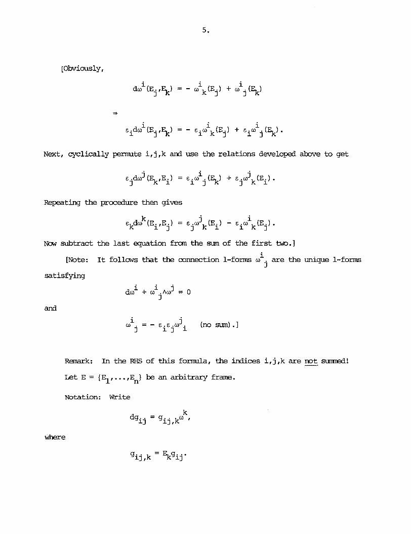
[Obviously,

s

i i i cido (Ejt$) = - E o (E.) + cia ( ) . i k l j 5

Next, cyclically permute i , j , k and use the relations developed above to get

Repeating the procedure then gives

Now subtract the l a s t equation fm the sum of the f i r s t t m . 1 i

[Note: It follows that the connection 1-forms o are the unique 1-forms j

satisfying

i i do + w .no' = 0

3 and

2 = - j

E . e . o j (no-).] 11 i

Remark: In the RHS of this formula, the indices i , j , k are not - surrsned!

L e t E = {EII..erE } be an arbitrary frame. n

Notation: W r i t e

Then

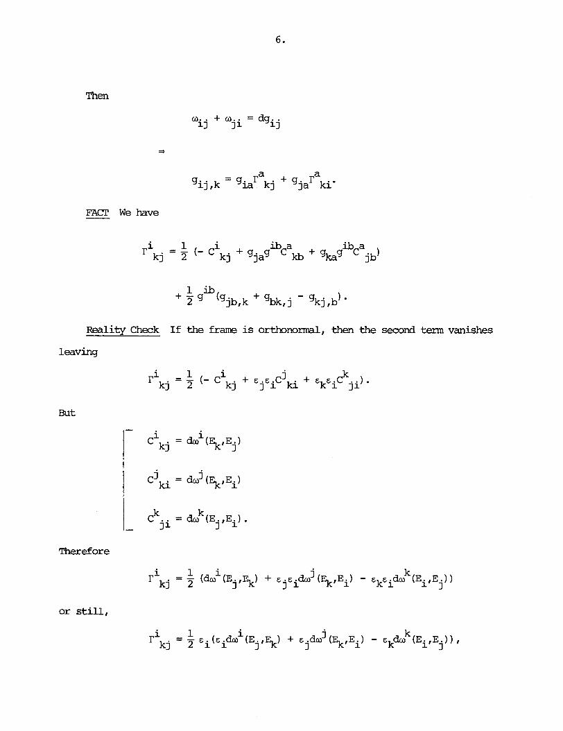
FACT We have

1 i ib a i b a rikj = T (- k j + gjag C kb + g k s C jb)

Reality Check If the frame is orthonormal, then the second term vanishes

leavhg

Therefore

or still,

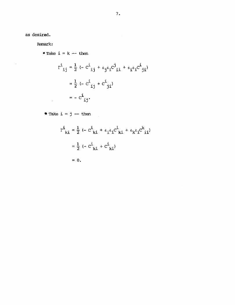
as desired.

Remark:

Take i = k-- then

- - - Ciij.

Take i = j -- then

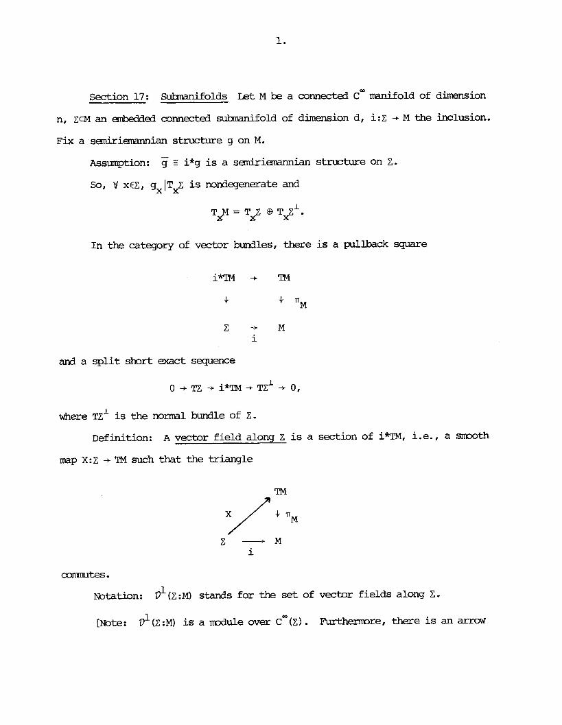
Section 17: SuhTlanifolds Le t M be a connected coo manifold of dimension

n, ZCM an embedded connected s-fold of dimension d, i : ~ + M the inclusion.

Fix a sesnirig~nnian structure g on M.

- Assumption: g i*g is a sernFriemannian structure on Z.

So, Y XCZ, gx I T ~ Z is nondegenerate and

In the category of vector bundles, there is a pullback square

and a s p l i t short exact sequence

where TZ' is the normal bundle of Z.

Definition: A vector f ield along Z is a section of i*TM, i.e., a mth

map X:Z -t TM such that the triangle

Notation: D' (Z :M) stands for the set of vector f ields along Z . 1

[Note : Q (Z:M) is a rrcdule over crn(z) . F'urth-re, there is an arm

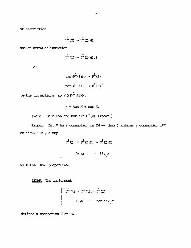
of restr ict ion

arad an arrow of

L e t

be the projections, so V x € v ~ ( Z : M ) ,

X = t a n X + n o r X ,

[Note: Both tan and nor are C-(2) -linear. I

Rappel: Let V be a connection on TM -- then V induces a connection i * ~

on i*TM, i.e., a map

I- 1 1 ~ ' ( 2 ) x D (Z:M) + D (Z:M)

w i t h the usual properties,

LFMW The assigrrment

(V,W) ----+ tan i*V? I - defines a connection 7 on n.

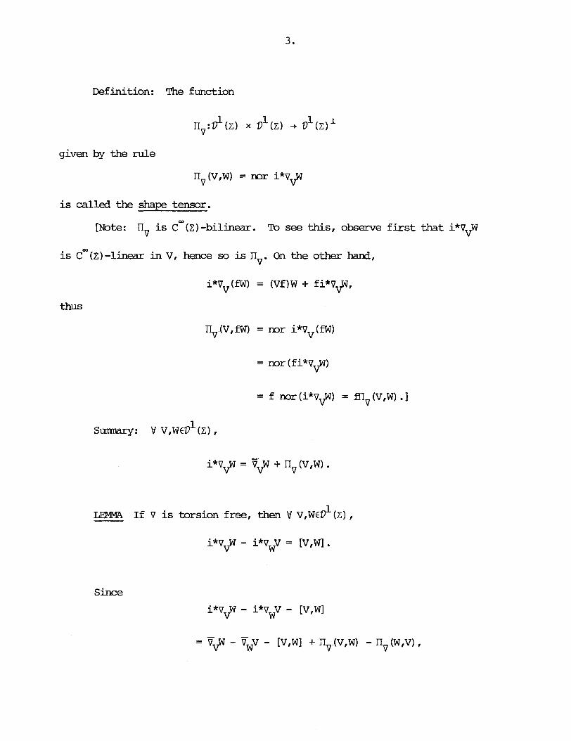
Definition: The function

1 1 1 nv:D (z) x D (z) - D (z)' given by the rule

IIv(vIw) = nor i*VvW

is called the shape tensor.

[mte: Tiv is cm ( 2 ) -bilinear. To see this, observe f i r s t

is cW(z)-linear i n V, hence so is nV. On the other hand,

i*$(fw) = (Vf)W + f ifV$.

thus

nv (v,fW) = nor i*Vv(fW)

= nor (fi*V$J)

= f nor (i*V#) = mV (V,W) .I

1 LEMMA If V is torsion free, then \y' V,W€D (Z) ,

i*V# - i*VwV = [V,W].

Since

it follows that i f V is torsion free, then is also torsion free and nV is

symuetric .

1 1 LEMMA Suppose that VEcon TM -- then W VED (z) , tl X,YED (Z:M), g

Application: W e have

VEcon TM =, %con TZ. 9 -

g

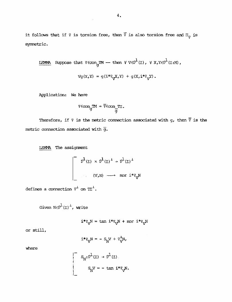
Therefore, i f V is the metric connection associated w i t h g, then 7 is the

metric connection associated with 7.

LEMMA The assignment

I defines a connection V' on TZ .

1 Given NED (z)', write

i*v$ = tan i*v$ + mr i*V$

or still,

where

Therefore, as e l m t s of Dl (Z) ,

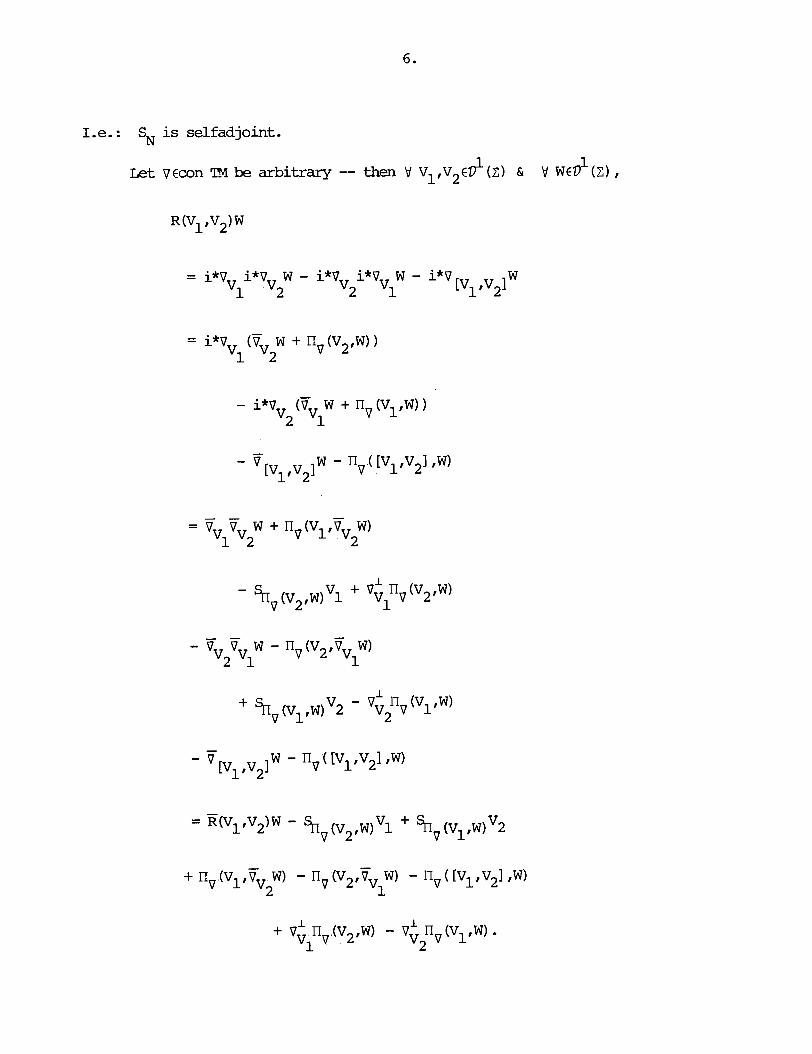
1.e.: SN is selfadjoint.

1 1 Let vccon TM be arbitrary -- then V V1,V2€D ( 2 ) & V WCD ( 2 )

W r i t e

and

Therefore

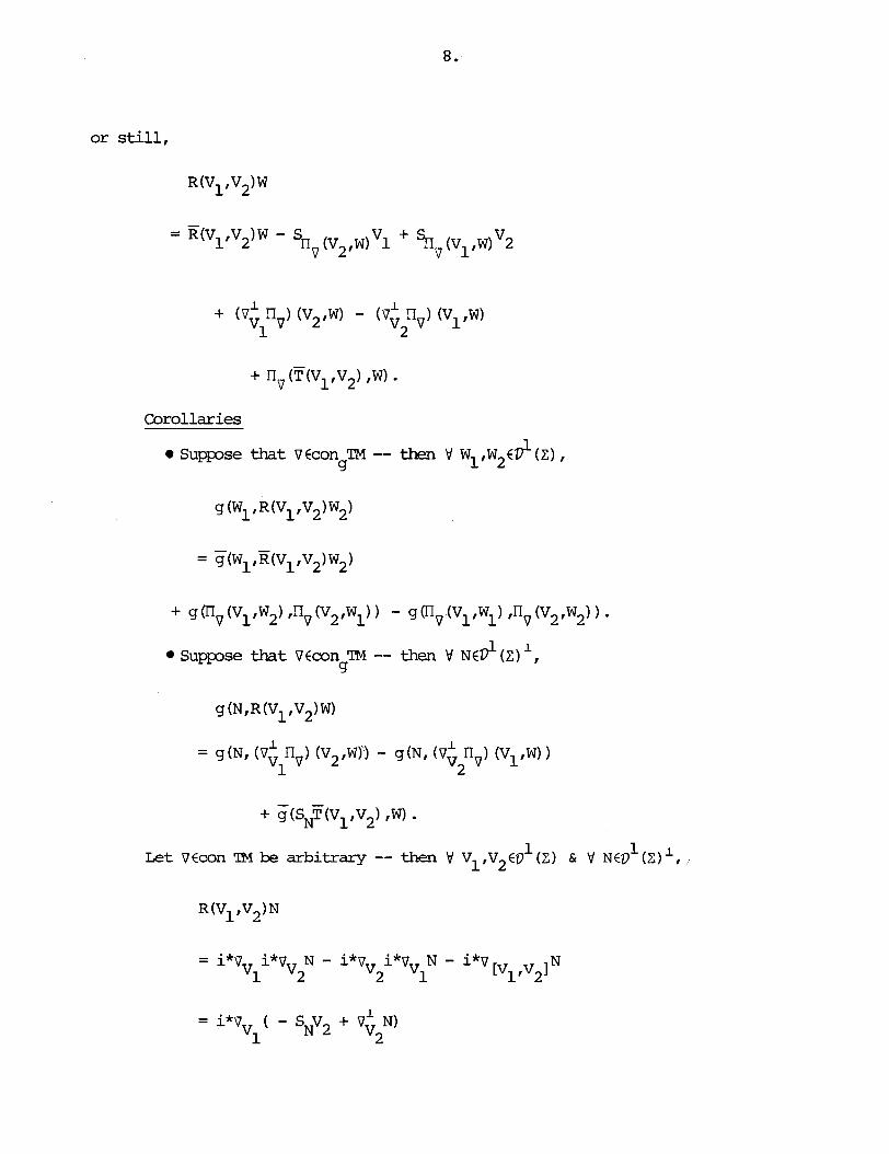
+ nv (T(V~,V~) rW) . Corollaries . Suppse that VCcon TM -- then V W ~ , W ~ € # (7,) ,

4

1 1 Let Vccon TM be arbitrary -- then V V1,V2ED (Z) V NCD (z) ',

where, by definition,

Corollaries

1 I S u p s e that V€mn TM -- then V N1,N2EZ) (Z) r g

1 0 Suppose that Vcwn TM -- then V WED ( 2 ) ,

53

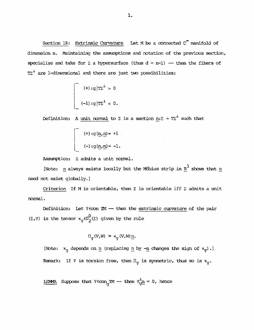
Section 18: Extrinsic Curvature L e t M be a oonnected cm manifold of

dimension n. Maintaining the assumptions and mtat ion of the previous section,

specialize and take for Z a hypersurface (thus d = n-1) -- then the fibers of

TZ' are 1-dhasional and there are just tm possibilities:

I Definition: A unit normal to Z is a section - n:Z -t TZ such that

Assumption: Z admits a un i t normal.

3 [Note: - n always exists locally but the Mbius s t r i p i n - R shows that - n

need not exist globally.]

Criterion If M is orientable, then Z is orientable i f f 2 admits a unit

normal.

Definition: Let Vfcon Tbf -- then the extrinsic curvature of the pair

0 V is the tensor xgEV2(Z) given by the rule

[Wte: xv depends on - n (replacing - n by -n - changes the sign of xv) .I

Resnark: I f V is torsion free, thenll is symwtric, thus so is x v v '

I IJiFMA Suppose that -- then Vp - = 0, hence

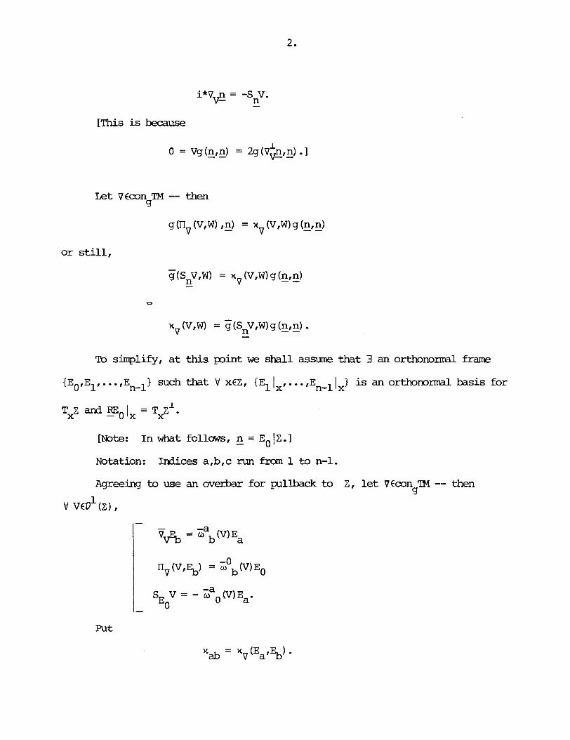
[This is because

Let VEcon TM - then 53

V vcvl (2) 1

Put

To simplify, a t this p i n t we shall assume that 3 an orthonorm1 frame

{EO.E1, . . . ,En - such that V xCZ, E . . . , E n 1 J is an orthomrmal basis for

TxZ and SO l x = T ~ Z ~ .

[Wte: In what follows, - n = ~ ~ 1 2 . 1

Notation: Indices a,b,c run from 1 to n-1.

Agreeing to use an overbar for pullback to 2, let VEcon -- then g

Then

- - - -b E E W ( E l Ob 0 a

-b -b -a w O = W ( E ) w 0 a

- - - -a & E X 0babw

*

-0 - -b - -a " b - - C E O Ob O - X a b O '

Remark: Suppose that v is the metric connection associated with g -- then

-0 &, = - ;o ,,;a = 0 a

=$

;O (V) ;a (W) = ;O (W) ;a (V) . a a

Therefore

xv (VfW) = E0& V,W Eo

-b = - (w)Eb)

- - - E E ;a (v) Ga(w) Oa 0

= ;O (V) ;a (W) a

= x, WIV) I

which confirms what we already knaw to be the case.

[Note: Similar considerations imply that the tensor

(VIW, - z Z o ( V ) gdo (W) a

is s p t r i c . ]

In anticipation of l a te r developoents, ass- henceforth that g T I n - l - and g 0

Let

0

w

(SO E~ = - l I ca =

VEcon TM -- then 4

[Note: The Zab are the connection 1-forms of 7 but the Eab are not the

curvature forms of V, these being the (n-1) ,a b'l

Suppose now that V is the metric connection associated with g (thus 7 is

the metric connection associated w i t h ;?) . LRt G be the Einstein tensor -- then

[The second relation is trivial. To check the first, note that

- 1 Goo - Roo - - 4 S

2 00

- - 2 1 Roo + 2 1 ZRaa.

a

On the other hand,

And

But

0 - b bob - - 'O'bR OOb

- b - OOb

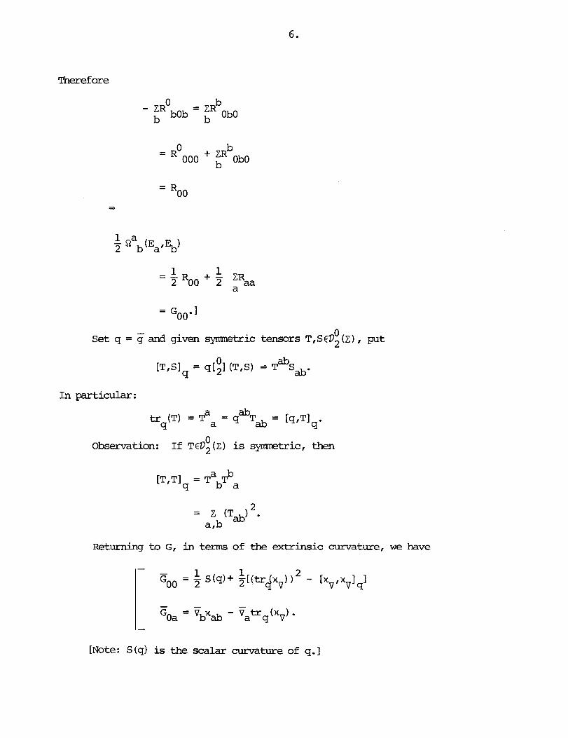
Therefore

0 b - ZR bob = ObO b

- 0 b - 000 + ObO

= Goo.]

- 0 Set q = g and given qmmetric tensors T, S€P2 (z) , put

0 ab [T,Slq = q121 (T,S) = T S*.

In particular:

0 Observation: If T E D ~ ( z ) is symetric, then

[Note : S (q) is the scalar curvature of q. ]

To begin with,

or still,

From the definitions,

Turning to the fonrolla for coa, write

We have

We have

minus

Since x is syrrunetric, v

But

or still,

Section 19: Hdge Conventions Let M be a connect& cm manifold of

dimension n.

Rappel: If cp is a density of weight 1, i.e., i f cp is a section of the

density line bundle Lden(M) -+ M, then one can associate w i t h q a Radon

measure m : cP

Let g €M - -- then 1 g 1 'I2 is a density of weight 1, from which rn lg 11/2'

Assunvt now thatM is orientable with orientation y -- then there is a unique

n-form wl €A% such that Y xCM and every oriented orthomrmal basis for TxMI g

vol (E ,...,E 1 = 1. glx 1 n

1 n [Note: In a connected open set UCM equipped w i t h coordinates x ,...,x

consistent w i t h p, i.e., such that

we have

1/2 1 ,, vol = 1CJ1 dX ... A ax".] g

Remark: Let z be a hypersurface (subject to the standing assumption

that g is a semiriernannian structure on 2 ) . Suppose that Z admits a un i t norm1

n -- then the pair (p,n) determines an orientation 'I of 2 and d -

Let XE+(M) -- then

LXvol = (div X)vol g g '

[Wrking locally, w e have

= (div X) vol .I g

[Note: By contrast,

VXvol = 0 g

i f V is the metric connection. Proof:

ox( 191 A . . . A dx")

Application: Suppose that X has rompact support -- then

.f (div X) vol = 0. M g

[In fact,

J (div X) wl = 1 pl M g M g

But c vol is a compactly supported (n-1)-form, hence x 9

I d ( L ~ V O ~ ) = 0 M g

by Sbkes4 theorem. I

0 = .f div ( fX) vol = J (Xf + f (div X) ) vol M g M 9'

or, in index rotation,

Example ( Y a m ' s Formula): Working w i t h the metric connection, l e t

= R . x k l = R i c (X,X) . a1

In the relation

div(fX) = fdiv X + X£,

take f = div X to get

2 div ( (div X) X) = (div X) + X (div X)

2 = (div X) + d(div X) (X) .

i Since div X = Xii, it follavs that

d (div X) (X) = ; i ;a-

Therefore

R i c (X,X) = x % ~ ;a; i - d (div X) (X)

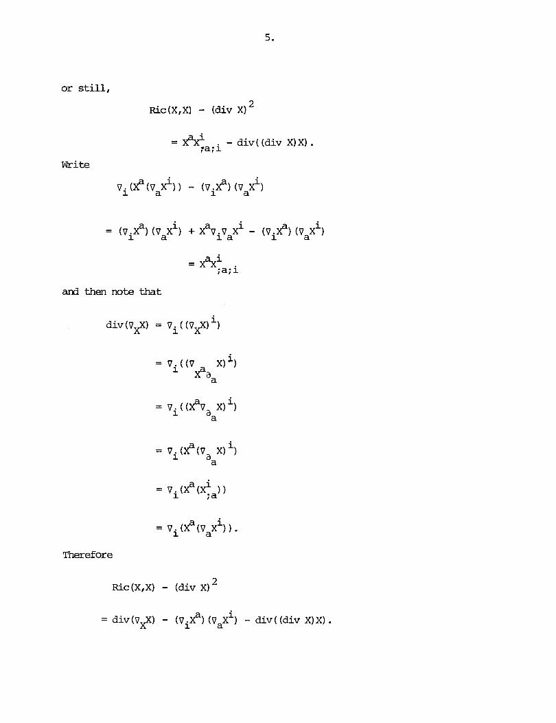
or still,

Ric (X ,X) - ( d i v X) 2

= - div ( ( d i v X) X) . ;a; i

W r i t e

and then note that

Therefore

Ric (X,X) - ( d i v X) 2

= div ( ~ $ 1 - ( v i e ) (vaxi) - div ( ( d i v X) X) .

Ric (X,X) - (div X) + ( v i p ) ( v a 2)

= div ( V s ) - div ( (div X) X) . To understand the term

(vie) (0~2) 1

1 recall that VX€Q1(M) or, equivalently,

thus

Claim:

equals

Indeed

So, i f X has ccgnpact support, then

Renark: We have

= c ( v j 2 + 0'24) (V.X. + V.X.) i, j 1 1 1 1

= z ( v j x i ) (VjXi) + z (v+) (V.X. , i, j i , j 1 3

* F r o m the definitions,

1 g $1 (vx, 0x1 = (vx) i j (,) ij

= cvjX=, ( V .X. ) . 7 1

Fram the definitions,

( v i A (v I 2)

= vmgj\v.xi 1 3

= v i x g j k o 3 .Xi

Therefore

FACT We have

[Observe that

The material in Section 3 can be applied to the t r iple (MIgI P) pointwise I

hence need not be repeated here.

This said, consider the star operator

* (div X) = (div X) vol = LXvd g g '

IXMMA L e t V be the mtric connection -- then V ~ € 9 (M) , the diagram

APM 2 An-',

comrrutes . [Fix p€.APM -- then V a€APMr

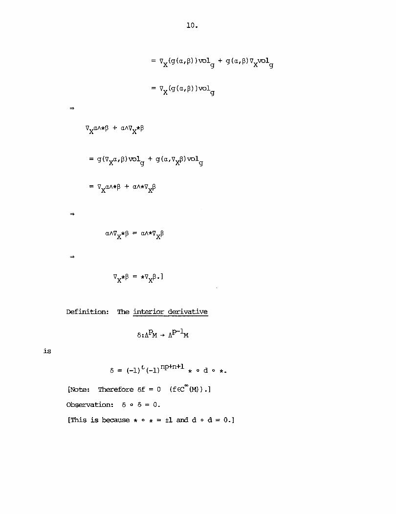
Definition: The interior derivative

[ ~ o t e : Therefore 6f = o ( f (MI ) . I

Observation: 6 0 6 = 0.

[This is because * 0 * = 21 and d o d = 0.1

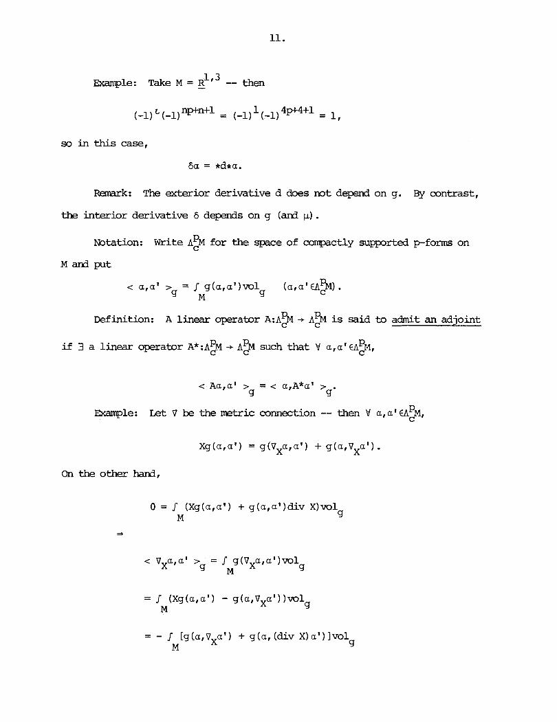
Example: Take M = - -- then

SO in this case,

6a = *d*a.

Remark: The a c t a i o r derivative d does rot depend on g. By contrast,

the interior derivative 6 depends on g (and p) . Notation: W r i t e AEM for the spice of ccarrpactly supported pforms on

M and put

Definition: A linear operator A : A ~ -+ A 9 is said to admit an adjoint

i f 3 a linear operator A* : A ~ M -+ A'M such that V a, a ' €A>, C

c Aa,af 7 = < a,A*af 7 g '

Ekample: Le t V be the metric connection -- then V a,af€AP,

Xg(a,af) = g(VXa,af) + g(a,VXat) . On the other hand,

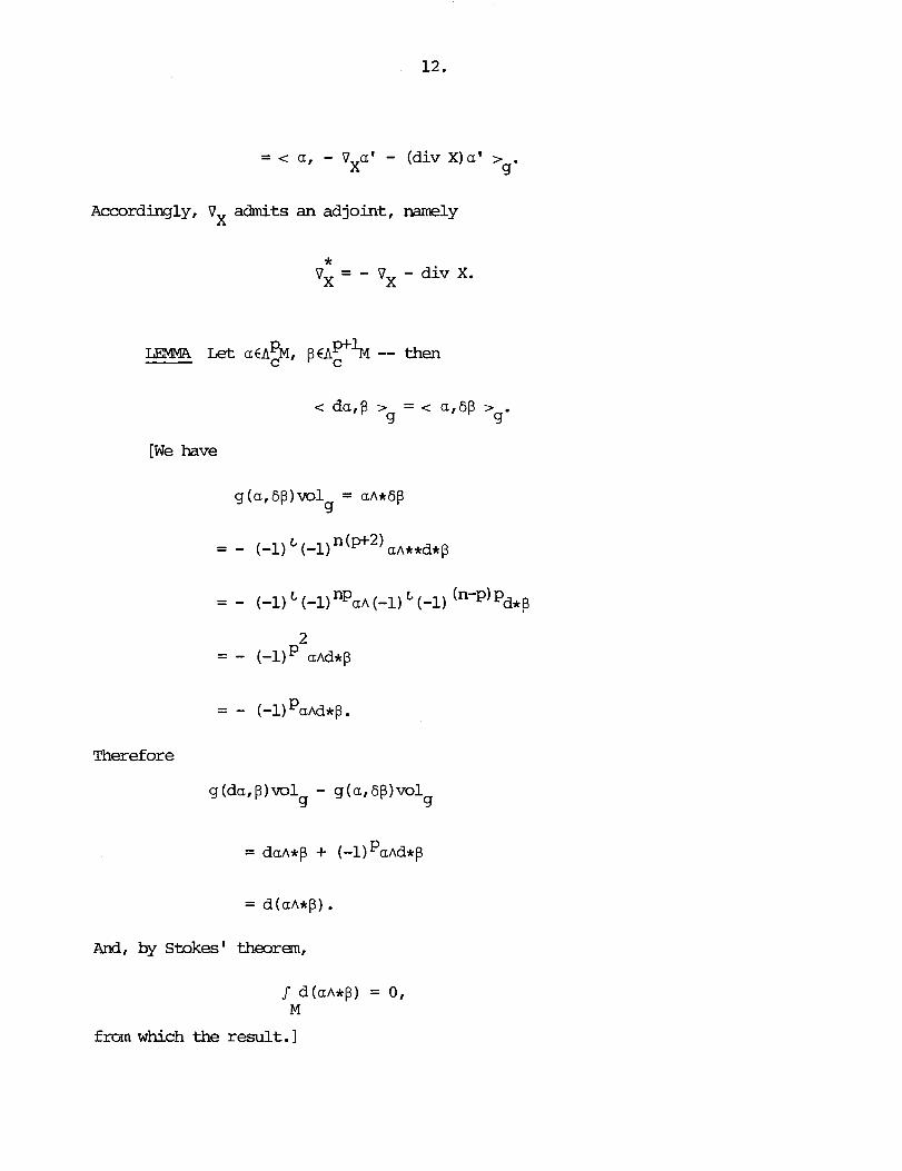
= c a, - VXaV - (div X)a' > 9 '

Accordingly, Ox admits an adjoint, namely

* - VX - - OX - div X.

T h e r e f o r e

g(da,P)volg - g(at6$)volg

And, by Stokes' theorem,

£ r a n which the result. I

Example: The Lie derivative %:A% + $34 admits an adjoint. Thus put

b E x = g X A - . Then

c L a,al 7 = I g(LXa,a')ml X M g

* L X = 6 0 ~ X + ~ 0 6 . X

[Note: Up to a sign, the composite

* p-P+l =z ,n-P *P A p - I +

is E 'Ib see this, let B€.Apb -- then X '

1 LEMMA L e t XED (M) -- then

div X = - &x.

[In fact, V f C C ~ (MI ,

div x = - 6gbx.]

Consequently, if a€Vl(M) , then locally

b 6a = Sg X = - div X

To generalize this, let ~ E A ~ ~ I (p > 1) -- then locally

hence

So, £ran the definitions, V $ €.Ap%,

But

is a divergence, hence integrates to

Restated, these considerations

N

zero. Therefore p = 6p.

lead to the conclusion that locally,

FACT V f (M) , -

6(fa) = - tdfa + f6a.

Recall m w that

A = div 0 grad

= div o g# o d.

Therefore

or still,

Definition: The laplacian

A :A%I -+ APM

is

A = - (d 0 6 + 6 0 dl .

Properties: (1) A = A*; (2) d 0 A = A 0 d; (3) 6 o A = A o 6;

(4) * o A = A o * .

FACT Let f €cm (M) , ~EA'M -- then

A(fa) = (Af)a + f(Aa) + 2Qgrad £a.

[Note: On functions,

A(flf2) = (Afl)f2 + f l ( A f 2 ) + 2g(grad fl,grad f2) .I

Definition: The connection ladacian

[Note: In other mrds,

which makes it clear that A,, is a metric contraction of v%. 1

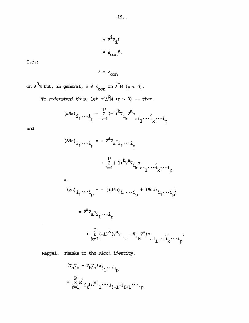
0 on A M but, in general, A # Aoon on AP14 (p > 0) .

To understand th i s , let ~CA'M (p > 0) -- then

( A d il--ip = - [ (dFa) . + (Fda) 1 il* -P 1- . ' lp

R a p 1 : Thanks to the Ricci identity,

or still,

Therefore

[Note: This is the so-called Weitzenboeck formula.]

Example: Take p = 1 -- then

Since the Ricci tensor is given by

we have

But

Therefore

i (Aa) = V ~ V a - R. a,.

j a j I 1

FACT On forms of degree n, A = Aeon.

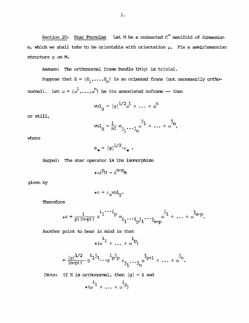
Section 20 : Star Fomlae Let M be a connected coo manifold of dimension

n, which we shall take to be orientable with orientation l ~ . Fix a senniriemannian

structure g on Mc.

Assume: The orthonormal frame bundle Ill (g) is trivial .

Suppse that E = &,...,En1 is an oriented frame (not necessarily ortho-

norrml) . Let o = {a1,. . . ,on} be its associated coframe -- then

or still,

where

Rappel: The star operator is the i m r p h i m

given by

*a = t,ml g '

Theref ore

Another point to bear in mind is that

i i *(a A ... n o P)

[Note: If E is orthonormal, then Ig

- - 1 & . . .Ei Ci . .i o n ... A w .] (n-p) ! il p 1 p p + l 0 * * j n

m@n Assume: p 7 1 -- then i i

P ( p - l ) S ( a l ~ ... n o

[We have

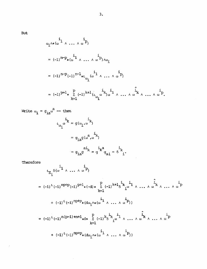
B u t

a Write wi = giaw -- then

Therefore

Since in general

it thus follows that

Remark: In principle, the levrma allows one to ccanpute

by iteration provided that p > 1. A s for p = 1,

i j = - div g E

j

So, i f E is orthonormal, then

- - - - eiCi (no sum)

m l e : Take p = 2 and suppose that E is orthomrmal -- then

or still, i i 1 2

i i il i2 6(o A ) = C 2 0 1 - C o

i i 1 2 + (-1) (doi" (a Aco ) ) .

W r i t e

do. = €.do i 1 1

Then

x det I

Therefore

[ ~ t e : =fine C- functions da by

Then the preceding considerations enable one to express

LEMMA Let V be a connection on TM -- then

[Note: The connection 1-forms of V per E are given by

and one writes

Recall too that

ij jki o = g wk.

To establish this result, it will be convenient to divide the analysis

into t w o parts.

S u p p o s e first that E is orthonormal -- then i i

P d * ( w A ... A o )

- - 1 E " * E E . d ( w

j n i i ...i j ... A w )

(n-p) ! il 1 pptl"'3n

i i P = d w a k ( o A . . . A o "aa)

a b i = ( 0 " - o b

i i = (o A . . . A o 'noa)

a b i - o bAco A* (w i

A . . . A w 'noa) . B u t

Agreeing to write

b a W = & E m a a b b (n0 sum),

it then follows that

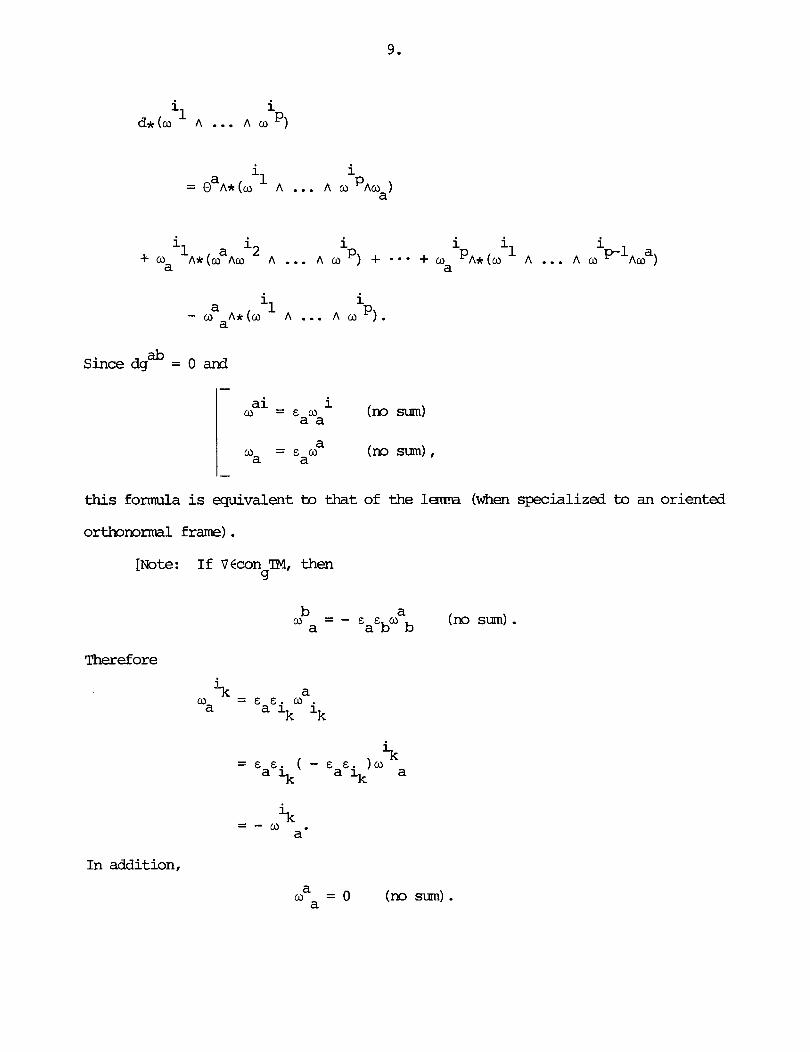
Since dg* = 0 and

i o = & a a a (no m)

this formula is equivalent to that of the l e ~ r m a (when specialized to an oriented

orthonormal frame).

[Note: If VCcon TM, then 9

b (f, = - a

E E O a b b (no sum). a

Therefore

In addition,

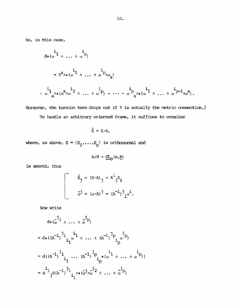
SO, in this case,

i i i i i i 2 p-1 a -olA*(oaAo A ... A m P ) - a - * - o P A * ( o 1 h ... Ao A w ) .

a a

fbreover, the torsion term drops out if V is actually the metric connection.]

To handle an arbitrary oriented frame, it suffices to consider

where, as above, E = (E,, ..., Em) is o ~ n o r m a l a d

i s mth, thus

Now write

-

where

Rappel: Under a change of basis E -t 6, the connection 1-forms compute as

Consider the torsion term:

From the definitions,

And

Therefore

A i a j b i a ' gjb = A A '

SUBLEMMA We have

[In fact,

Therefore

Next, consider

Since the treatment of each term is the saxre (up to notation), it suffices to

deal w i t h

or still,

or still,

We have

And

Finally

3, Retaining the differential dg , the claim then is that

But this is clear:

It remains to consider

or still,

To proceed fran here, simply observe that

1 4 3 - =;j - 3 g dg*.

j

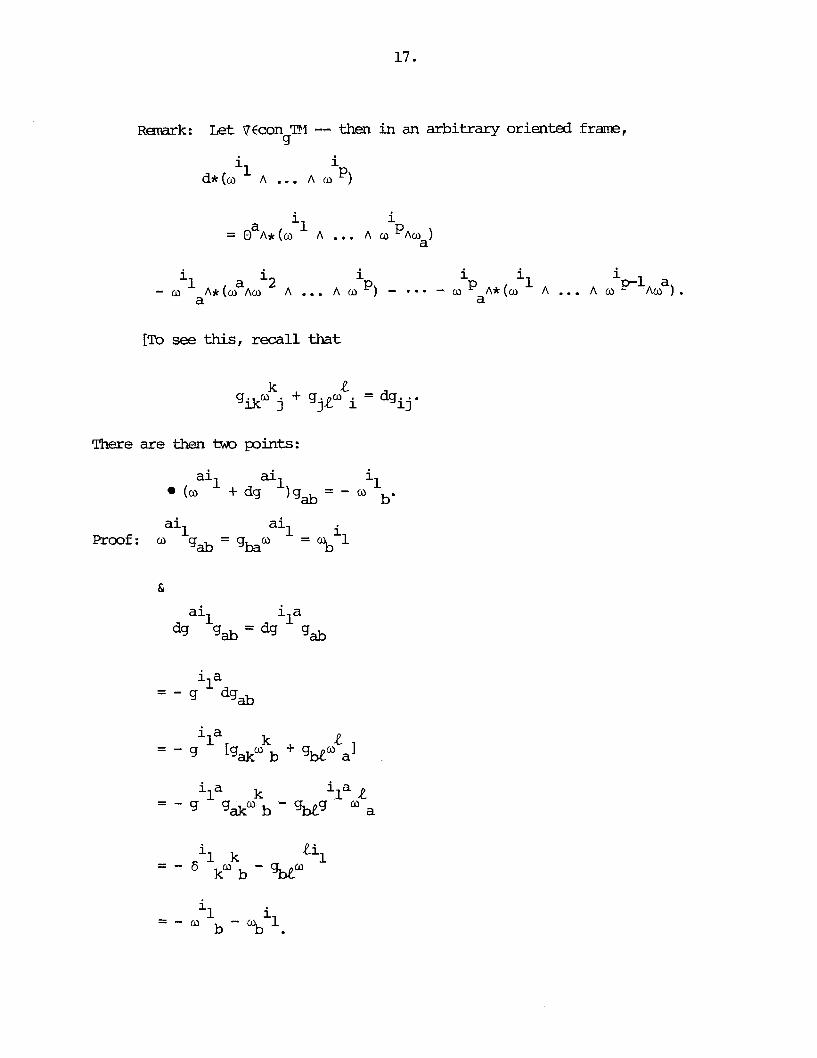
ema ark: Let VCcon PI -- then in an arbitrary oriented f ram, g

i i d*(a A ... A a ')

[To see this, recall that

There are then Ism pints:

ai 1 ai Proof: a g * = g d

1

ai 1 i a 1 d9 9, = dg gab

1 ab Proof: - 2 g dg*

- - - - 1 b a a 2 [ ~ ~ + a ~ l = - f-0 a -1

Suppose that E is an oriented orthomrmal f r m and take for V the metric

connection.

i j i LEMMA Put o = e . w (m sum) -- then 3 j

i j j i oij = (-1) % [*do A o - *do A o

k k i j ( - 1 Zek* (do A o ) A o A o I . + Z k

Since

we have

Therefore, i n t e r m s of the interior product,

B u t

k k ( d o A o ) (E E X)

i' jf

k k ckdo (EifE.)w (X)

3

k k Zekdo (Ei,E .)a (X) k 3

i j k k = - cido (E X) + &.do (Ei,X) + Zck(dw A o ) (EirE X).

j ' I k j '

From this, it follows that

1 k k do' - - % L ~ , L~ ( d o A o ) ) .

3 i

Rappel : v x ~ p l (MI , Y a C A ~ M ,

Then

[Note: Because it is a question of an ortbmrmal basis,

Let

Then

k k k k i (do A a ) = (-1) ' (-1) "-I* (* (do Am ) Asia ) .

Now put

Since fl is a 2-form,

However

Thus

k k i j = (-1) ' (-1) n-l(-l) (-1) L* (* (do AW ) Asia As .o ) I

Putting everything together then gives

as asserted.

Section 21: Metric Cancornitants L e t M be a connected cm manifold of

dimension n.

Notation:

are charts with tTf~#fl such tha t

[Note: In th i s section (as w e l l as sane others to follow), it w i l l be

m r e convenient to use bars rather than primes to designate a generic coordinate

change. 1

Put

Then

Assume now thatM is orientable -- then the set C of coordinate systems +

on subsets of M sp l i t s as a disjoint union C+UC- such that within C or C- one

always ' has

i J = det[J kl > 0.

Definition: A semitensor of type (p,q) and weight w is an entity

satisfying this condition within either C+ or C- , i. e. , for coordinate changes

subject to J > 0.

If w-s@(M) is the set of such, then 4

[Note: The tensor transformation rule for the sections of T'(Y) 63 L ~ ( M ) 9

W involves I J I , while the tensor transformation rule for the sections

T' (MI @ L:= (M) involves sgn J- I J I W. Thus, i n ei ther case, a generic 9

J.

of

section

is a semitensor of type (p,q) and weight w. For example, i f g€M, - then

- e *

are semitensors of type e g -

Definition: A metric c o n d t a n t of type (p,q), weight w, and order m

- (n, 0)

and weight 0 but, being Wisted, are - (0,n)

not tensors of type

is a map

- (n, 0)

- 1 (0,n)

i ... i for which 3 real valued coo functions F 1 P of rea l variables

jl= * jq

I . . . , X 1 n

xab~ ab,cle -c such that i f (U , (x ,..., x ) I is a chart, then ab,cl m

the ccPnponents of F (g) are given by

where the ccmm stands for part ial differentiation, i.e.,

i ... i [Note: The functions F 1 P are mt unique, thus equality of

jl- *jq

tm metric concartitants mans their equality as mps f ran Pa - to w-s$ (M) . I q

Rgnark: The index scheme is mt set i n concrete and depends on the

situation, e.g., to free up a,b,c one can use r,s,t:

Notation: MCn(pIqIw,m) is the set of mtric concanitants of type

(p,q)[ weight w, and order m. With respect to the obvious operations, M2(pIq,wIm)

is a real vecwr space.

[Note: In general, .%n(p,q.wIm) is inf ini te dimensional but, undw certain

interesting circumstances, is f in i t e dimensional (or even t r iv ia l ) . I

Example: The assigmnent g -r l g 1 'I2 defines an elanent of Kn (O.O.1,O) .

defines an elanent of MCn (p,q,w + W,m) .I

-1e: Given g€M, view the curvature tensor R(gl attached to its

0 metric connection as an elment of D4(M) -- then the assignment g -+ R(g) is

a metric concomitant of type (0 ,4 ) , weight 0, and order 2. Indeed,

Therefore Ri jlce is linear i n the second derivatives of g (but nonlinear in the

f i r s t derivatives of g) . I

[Note: Recall that

Accordingly,

ema ark: Entities such as / R ~ ~ R . . j are not metric concanitants. 11

To reflect the underlying symnetries of the situation (s-ng f r m

the equality gab = gk), one can a s s m without loss of generality that a l l

internal indices have been symwtrized.

Example: Suppose that n = 2 and let F(g) = d e t g, a scalar density of

weight 2, thus local ly

H e r e we can take

or , i n accordance with the foregoing convention,

In the f i r s t s i tuat ion

but i n the second si tuat ion,

L e t F W n (p,q,w,m)

are related by

-- then the barred and unbarred components of F(g)

[Note: Differentiation of the tensor transformation rule

leads to the transformation l a w for the derivatives of gab. To start the

process, let

Then we have

N e x t , let

Then we have

And so forth... .I

Remark: Fix indices

and suppress them fram the notation. Let

and

Then, in general, the derivatives

are not tensorial. However, it is possible to construct tensorial entities

from certain canbinations of the A ab,... which turn out to be the ccpnponents

of metric concomitants

these being the so-called tensorial derivatives of F(g) . [Note: A particular case of the construction is detailed later on when

we take up the theory of lagrangians but, in brief, the procedure is this.

With the derstanding that covariant differentiation is per the metric

connection of g, the difference

involves the connection coefficients r' , their derivatives, and the h*, . . hab,cl- -ce (e c k) . Successive substitution of these f o d a s (beginning with k = m and ending with k = 1) then enables one to write

n*: This coefficient represents an element

where ... involves the connection coefficients I" their derivatives, and . . ab,cl-=-ck

the A (k = l,... ,m).

ab,cl= 0% . n : This coefficient represents an elanent

and

where ... involves the connection coefficients I" , their derivatives, and . . ab,cl--*cL

then ( L 7 k) . [Note: If k = m, then

It is not difficult to wmpute the tensorial derivatives when m = 1 or 2

but matters are mre complicated when m = 3. I

To avoid trivialities, in what follows we shall assume that n > 1.

Ll3lMA Let FCM3n(0,0,0,0) -- then 3 a constant X such that F = A.

[To begin wi th ,

~ ( 9 ~ ) = F'gab)

or still,

F d-a~sbg*) = F (g*)

Now differentiate this relation w. r . t . Jik :

- r k s s k aF (6 i6 aJ bgrs + ~~~6 i6 bgrsl = 0 -

i Specialize and take xi = x -- then Jrh = 6rb, hence

Therefore F is a constant, as clainaed. I

Application: If F ~ n ( O , O , l , O ) , then 3 a constant X such that

[Consider the quotient F (g) / 1 g 1 li2. I

LEWA If n is even and p + q is odd, then

-i - i Since n is even, we can take x - - x . Tkis gives

But

- - gab.

Therefore F = 0.1

FACT If p + q is odd and less than n, then

-Kn(p,q,w,0) = to)

Structural Considerations

*Let FEMCn(OfqfO,O). Assume: q is odd and q c n -- then F = 0.

*Let FWn(O,n,O,O). Assure: n is odd -- then

here L is a constant.

*Let FWn(O,q,O,O). .4ssune: q is even an3 q < n -- then

where the K are constants. o

.let FWn(Ofn,O,O). Assume: n is even -- then

where the KO and L are constants.

R m k : Due to the symmetry of g and the cammtativity of multiplication,

the decomposition

contains redundancies, there being

distinct terms (after canbination of the constants).

Example: Le t F@C4(0,4,0,0) -- then

where K1,K2,K3,L are constants.

Emnple: L e t FEPIIC4(0,4,0,0). S u p s e that

Then

where K and L are constants .

Remark: The situation when q > n is m r e involved. To i l lus t ra te ,

PC2 (0,4,0,0) contains elements of the form

[Note: Using classical invariant theory, one can express an arbitrary

element of MCn ( O , q , 0.0) (q > n) i n terms of products of the gij and lower

Levi-Civita symbols. ]

While formulated covariantly, a l l of the preceding results admit contra-

variant counterparts.

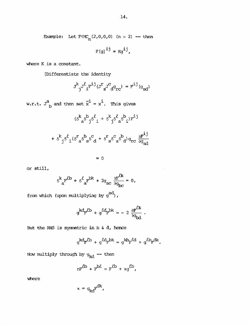
Exanple: L e t F ~ n ( 2 , 0 1 0 , 0 ) (n > 2) -- then

where K is a aonstant,

[Differentiate the identity

a i w. r . t . J and then set G~ = x . This gives b

k L r c b +6 .6 i (6ra6bs6cd+6 6 6 ) g - 3 s a d rc agsd

or still,

ad from which (upon multiplying by g )

aF Rk

% b + g 9 k = - 2 - . 9 agbd

But the RHS is syrranetric i n b & dl hence

Now railtiply through by gM -- then

where

or still,

Rb ( n - 1 ) ~ ~ + = xg . w solve for Pr mte that

To see that x is a constant, substitute back into the differential equation, thus

1.e.: x is a constant.]

[Note: If FWn(2,0,1,0) (n > 21, then 3 a constant K such that

F (g) i j = K 1 g 1 1/2gij (apply the above analysis to the quotient F (g) / (g 1 'I2) .I

Exmple: L e t FW2(2,0,0,01 -- then

where K and L are constants.

[From the preceding example, w e have

a + = xgb,

thus

Therefore

Since the LHS of this relation is skew symnetric in k & 1, it follows that

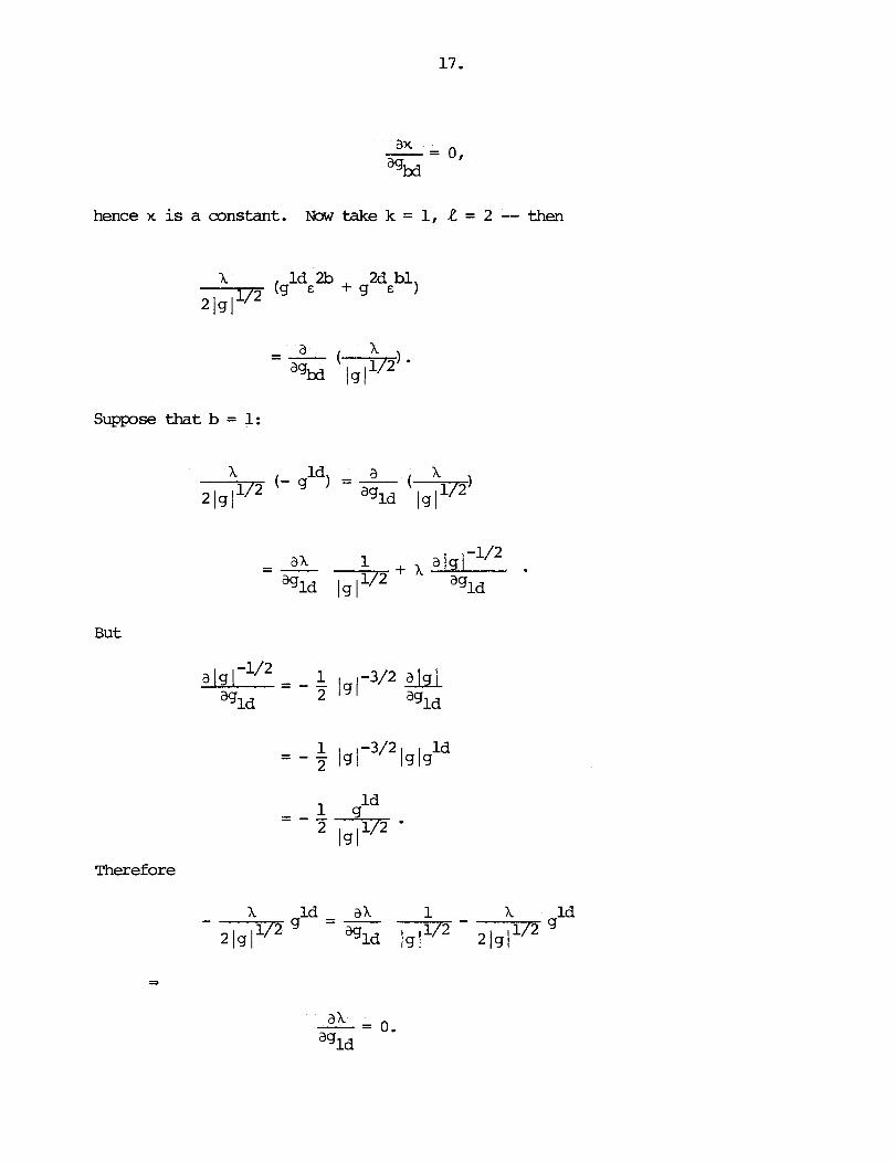
hence x is a constant. Now take k = 1, L = 2 -- then

Suppose that b = 1:

But

Theref ore

The same argument shows that

Conclusion: X is a constant. I

[Note: If F€lC2(2,0,1,0), then 3 constants K and L such that

i j 11/2gij + LE (apply the abxre a n a l y s i s to the q u o t i e n t

m l e : L e t FcX4(6,0,1,0). Suppose that

acbr st a s c b r t +K3(g g g + g g g 1

ab crst rs tabc) + L1(g + g E

as crbt + g r b , h y + L3 (g E

+ L4 (g at E crsb + g rc E

bc arst st rabc + L5(4 E + g & 1

whre I$ k = l f f l 1 ) and Le ( = l f f 6 are constants.

[Note: The quantity g ra E *st has the required symnetry but there is no

contradiction since

as crbt rb tasc - (g E + g E 1

ac brst rt sabc) - (g E + g E

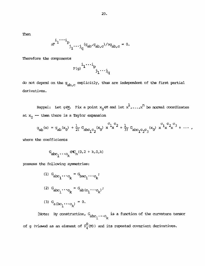
Then

Therefore the camponents

do m t depend on the g ab,c

explicitly, thus are irdependent of the first partial

derivatives.

1 n Rappel: Let g€M. - Fix a pint xo€M and let x ,..., x be mnml ccordinates

at x -- then there is a Taylor expansion 0

where the coefficients

possess the following synmetries:

[Note: By construction, Gabc is a function of the curvature tensor 1. OCk

0 of g (viewed as an element of D4(M)) and its repeated covariant derivatives.

and

THEDREBI L e t FblCn(pIq,w,m) -- then

Example: If n is even and q is odd, then

[Let F ~ n ( 0 , q , w , 2 ) -- then

i s i n c e n is even, we can take zi = - x . This gives

But

and

Therefore F = 0. ]

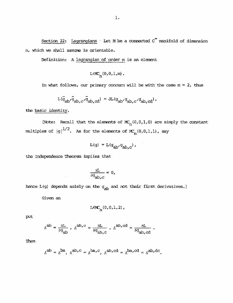
Section 22 : ~agrangians Let M be a connected C- manifold of dimension

n, which we shall assume is orientable.

Definition: A lagrangian of order m is an elanent

In what follows, our primary concern w i l l be with the case m = 2, thus

the basic identity.

[Note: Recall that the elmmts of X n ( O , O , l , O ) are simply the constant

multiples of l g ~ ~ ' ~ . As £or the elements of ~ ( O , O , 1 , 1 ) , say

the Independence Theoran implies that

hence L(g) depends solely on the g* and not their f i r s t derivatives.]

Given an

L~Wn(OIO,1'2) I

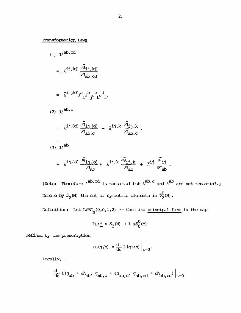
Transformtion Laws

[Note: Therefore A is tensorial but A and A* are not tensorial. ]

0 Demte by S2 (M) the set of symrtetric elements in D2 (M) .

Definition: L e t LWn(OI0,1,2) -- then its principal form

0 PL:M - x S2(M) + 1-sDo(M)

defined by the prescription

PL(g,h) = !!- L (g+&h) d&

is the IMP

0 [Note: To check t h a t PL(g,h) is an elenent of 1-sVO (MI , use the foregoing

transformation laws:

H e r e it is necessary to keep i n mind that the terms figuring in the transformation

laws for g and its derivatives are precisely the terms figuring in the trans- ab

formation laws for h and its derivatives. For instance, ab

= 9 i k j P + J ~ ~ P ~ ~ . ~

Remark: In reali ty,

is meaningful only i f h is compactly supported, the difficulty being that, in

general, g + ~ w - rm m a t t e r the choice of E # 0. E.g.: Take M = R, - let g be

the usual metric, and consider g+sh, where hx = xgx -- then a t x = - I/&,

%/& + 6 ( - V E ) ~ - ~ , ~ = 0.

Thus, s t r i c t ly speaking, the introduction of

d &- L (g+&h) (&=O

serves merely to mt iva te the definition of PL(g,h) .

L e t conOTM stand for the set of torsion free connections on TM.

Rappel : If V EconOTM and hES2 (M) , then

= h hij:k i j , k - I ' a ~ j - rajkhia

and

- - hi j ;M hij ,M - raikhaj,l - ra jk h ia,L - h a j - r a jk,L h ia

Given V€conoTMr define II i j ,k v by

. . and define by

the picture and set

, i j M = , i j M v

LF&MA V hcS2 (MI , we have

[That these expressions are equal is simply a computational consequence

of the definitions.]

DOL: This is the map -

ab with canpnents TIv .

DIL: Tkis is the map -

D2L: This is the map -

Rappel: Let g W - -- then the connection coefficients of the metric g connection V are

The tensorial derivative of L w.r.t. g is the el-t ab

The tensorial derivative of L w.r.t. g a, c is the element

defined by

When wrking locally, the tensorial derivatives of L w.r . t . g ab' gab,cr

ab *ab.d gab, cii w i l l be denoted by rI ,

On the basis of the definitions,

In addition to these e l m t a r y symetsies, there are two others which l ie

deeper, viz.

LEMMA W e have

rpb,cd + p , d b + nad,bc = 0.

[Consider the basic identity

- - - L(gij.gij ,kIgij,ke) = JL(gij.9ij $ 1 9 ~ ~ ,u 1.

- - - Using the transformation laws, express gij, gijIk, gijIke in terms of gab,

gab,c' gab,cd' the result being an expression on the IdlS involving fs, 6,. J~~~~ (the IWS is, of murse, independent of these variables) . Now differentiate

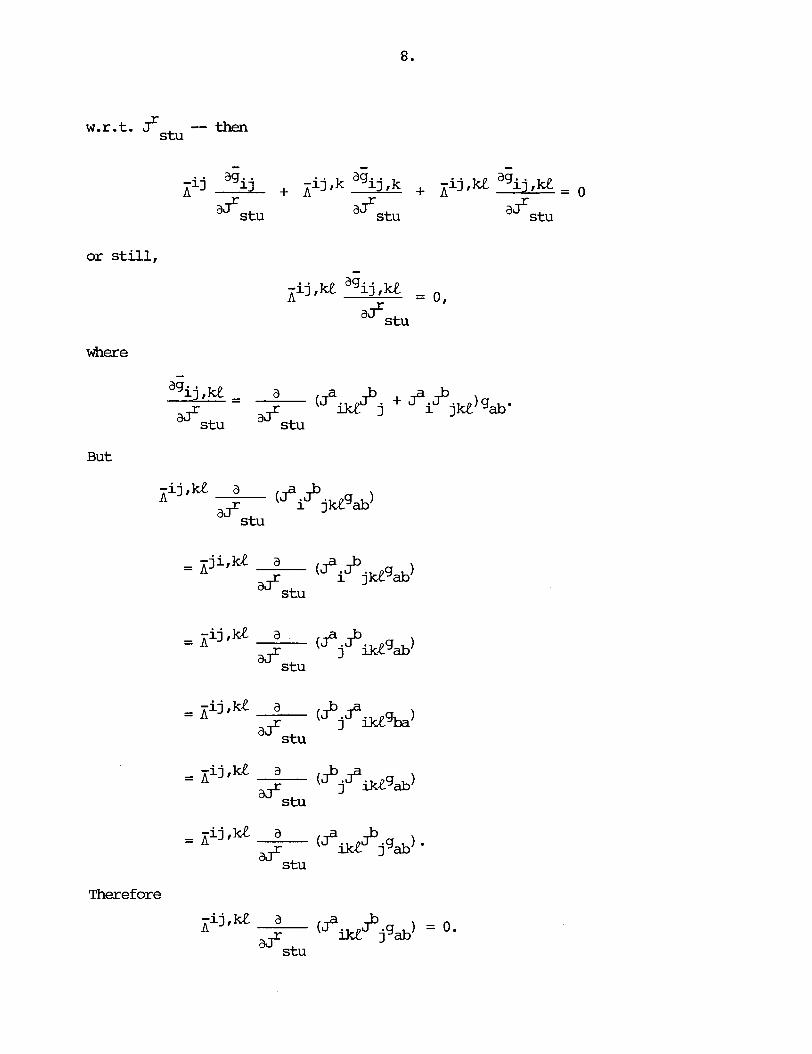
or still,

where

But

iiij ,ke a a 3

(fiPjlce9*) stu

- j i ,k l a = A

a f stu

- i j ,k l a = A

a? stu (Ja jPMg,)

- - i i i j ,kl a a? stu

- - i i i j Ik l a a?

stu

- - x i a (PikZj9*). a? stu

Therefore

x i j ,kl a d (~~,Jb~g*) = 0. stu

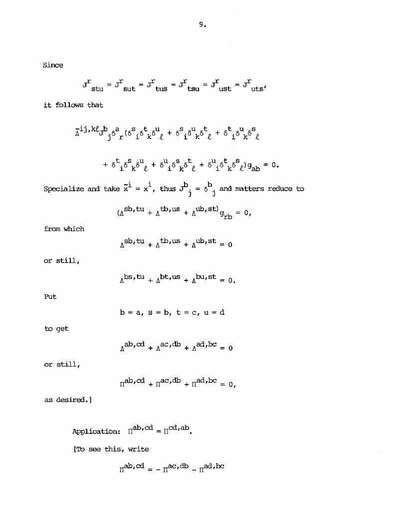
Since

2 stu =s sut =f tus =&=f ust =futs,

it follows that

-i - i b Specialize and take x - x , thus p; = 6 , and matters reduce to

£ran which

or still,

Put

to get

or still,

as desired. 1

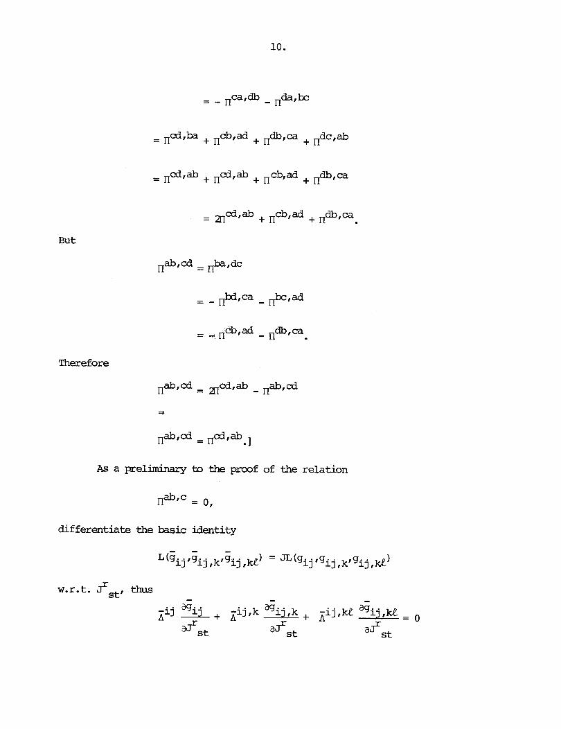
But

As a preliminary to the proof of the re la t ion

differentiate the basic identity

w . r . t . f thus - - - -ij agij A --- + ,-ij,k agijfk -ij,kL a g i j f ~ - + A - 0

"'st afst a*st

or still,

H e r e

and

NOW do the math a then take zi = xi to get

sb, t *rS = 0. + A grb + A grb

Fix a point x EM and introduce normal coordinates a t x -- then 0 0

gij,k = 0, hence at xo,

so from the above,

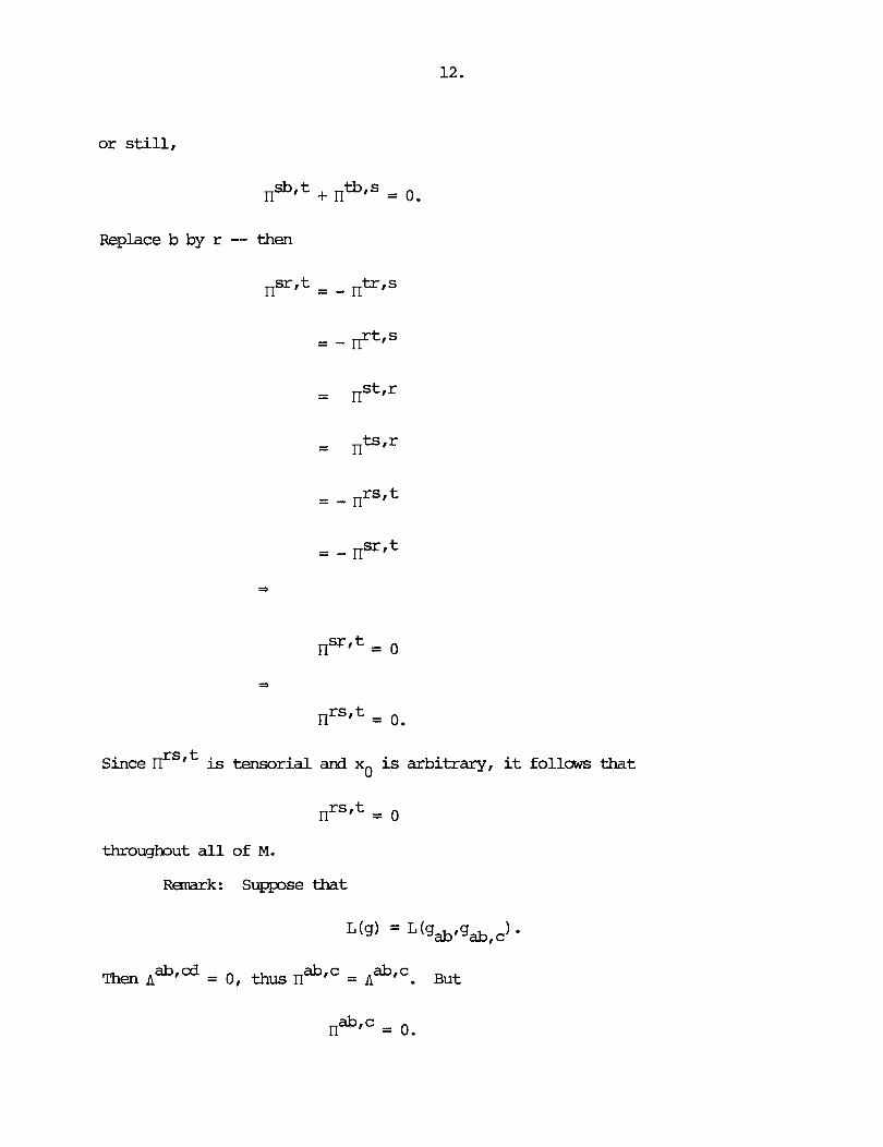
or still,

nsbrt + , = 0.

Replace b by r -- then

$Gt = - ,-,s

- - - ,rt, s

- - ,+r

- - p , r

- - - ,rs&

= - n sr, t

nsr,t =

*

,rs, t = 0.

Since ll rs, t is tensorial and xo is a r b i t r a r y , it follavs that

nrs, t = 0

throughout al l of M.

Remark: Suppose that

L(g) = L(~*,S*,~'

then^ *I* = 0, ttm n *tc = A*,c. ~~t

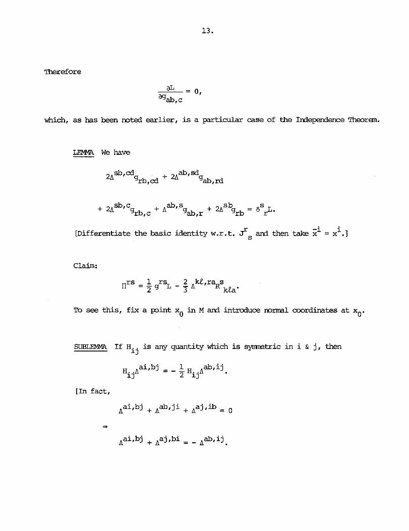
Therefore

which, as has ken mted earlier, is a particular case of the Idependence Theorem.

LEMMA We have

i [Differentiate the basic identity w.r . t. f and then take zi = x .I

Claim:

Tb see this, fix a pint x in M ard introduce r a m 1 coordinates at x0. 0

s- If Hij

is any quantity which is symnetric in i & j, then

[In fact,

A ai,bj + Aab,ji + Aajfib = o

Theref ore

A t Xo1

And a t xo,

or still,

Step 1:

Step 2: A t xo,

B u t

Therefore

as,kt - rrak,l!

- 1 rb as,kL - - 2 4 gab,&

1 rb as,M 1 rb as,U - T g ghk,a$ 'Tg gaklhtA

Write

1 rb as,kL - z 9bk,dA

- 1 rb sa,kL - - zg 4bk,aeA

- 1 rb sk,d - zg gbk,d

- 1 rb sa,U - as %,k@

- 1 rb as, ke - r g %,ken

Write

1 rb =#kt 2 4 gak,htA

Therefore

Interchanging r and s , w e thus conclude that a t xo,

Step 3: At xo,

and

Therefore

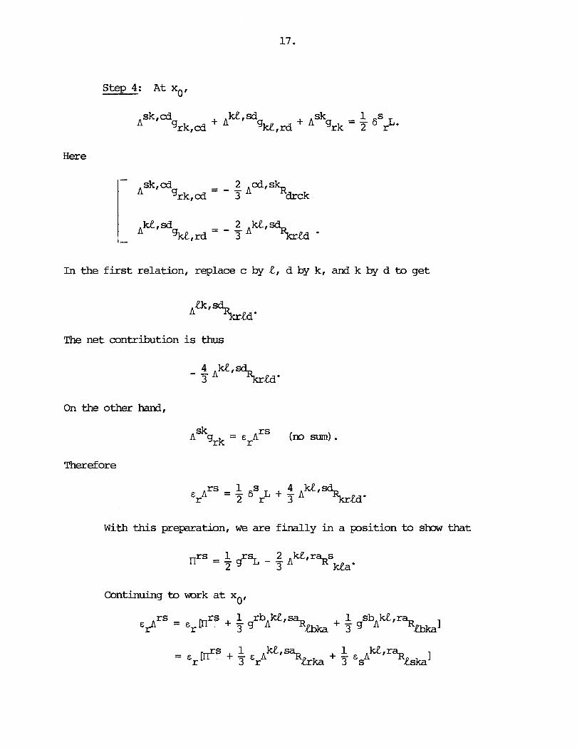
Step 4: Atxo ,

In the f i r s t relation, replace c by 1, d by k, and k by d to get

The net contribution is thus

On the other hand,

Therefore

With this preparation, we are finally i n a position to shar that

Continuing to mrk a t x 0'

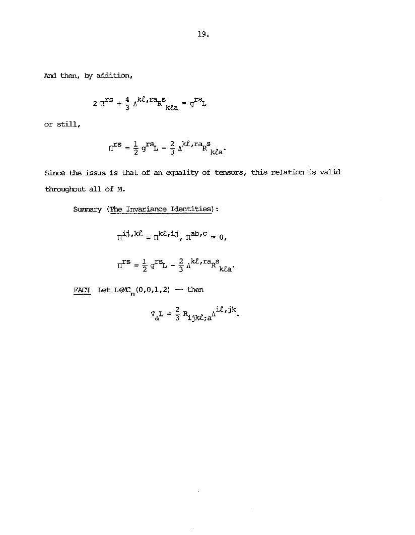
And then, by addition,

or still,

Since the issue is that of an equality of tensors, this relation is valid

througbut a l l of M.

Sum~lry (The Invariance Identities) :

FACT L e t LEM3n(OtO,1,2) -- then -

Section 23: The Euler-Lagrange Qyations Let M be a connected C-

manifold of dimension n, which we shall assume is orientable.

Definition: The Ner-Lagrange derivative is the map

E:MCn(O,O,ltm) + MCn(2,0,1,h)

given locally by the expression

[Note: It is cl- that Eij(L) is symnetric. However, since the definition

involves n o n t ~ s o r i a l quantities, it is not ccanpletely obvious that Eij (L) is

actually tensorial. In the case of interest, viz. when m = 2, th i s w i l l be

verified below.]

One then says that L satisfies the Euler-Lagrange equations provided

E(L) = 0.

Example: Let I, = I ~ ~ ~ / ~ s (S the scalar curvature of g) -- then (cf. infra)

But

* (G = Ein)

Therefore E(L) = 0 i f f the Einstein tensor of g vanishes identically.

[Mte: H e r e , (L) is of the second order in the gij and m t of the

fourth order (as might be expected) . I

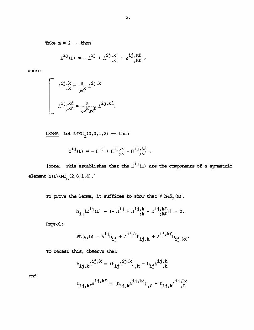
Take m = 2 -- then

LEBWi L e t L ~ n ( 0 , 0 , 1 , 2 ) -- then

[Note: This establishes that the E ~ ~ ( L ) are the ~ o ~ c ~ p o n e n t s of a symnetr ic

el-t E(L) Wn(2 ,0 ,1 ,4 ) .I

To prove the l-, it s u f f i c e s to show that V hCS2(M),

Rappel:

To recast this, observe that

and

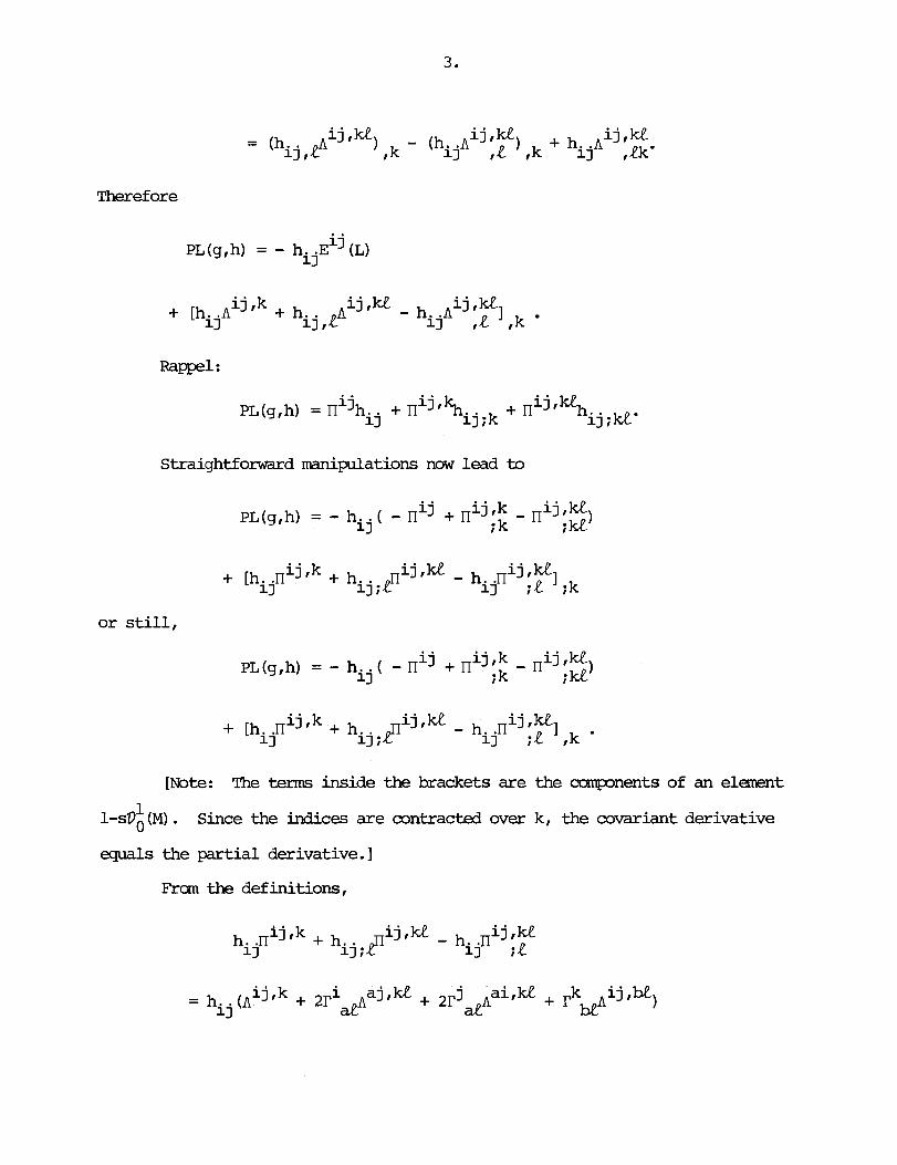
- - (hij ,p ijlke) - (h. .A ijtkL) +h. .A i j , k ~ 1 k 1 3 1.e tk 1 3 I&'

Therefore

i j PL(g,h) = - h. .E (L) 1 3

i j ,k + [h. .A i j ,ke - h. .A

i j ,ke 11 + h i j ,P I 1 3 1.e ,k

Rappel :

Straightforward manipulations now lead to

+ [h. .nijtk i j W - h. .n i j ,kL 1 3 + hij .F I 11 ;R ;k

or still,

+ [h. .rI i j ,k i j ,ke + hij ;p - h a II

i j MI 1 3 1 3 ;a. ,k '

[Note: The terms inside the brackets are the ccanponents of an e l m t

1 1 - s D O ( M ) . Since the indices are contracted over kt the covariant derivative

the partial derivative.]

E'rcxn the definitions,

i aj,kL = h . . (bijtk + 2r &A j a i , k e + $ ,ij.h.t) 1 3

+ 2r &A be

But

Therefore

i j = h . . ~ (L) - [ h . 2 j t k Ai j Iu - .A i j ,kt

11 11 + hij ,e I 13 I.e Ik

Since ijfk = 0, it follows that

or still,

[Note: Recall that

where X is a constant. Lacally,

and

In accordance with our syrranetrization convention, write I-

Then

w i t h

1 i j k t + , , , , i j k L I = g (6 a6 d6 b6 j + 6 i 6 j g k 6 L + 6 6 6 6 d a b c a d c b d a c b

i j k R j + 6i ,j 6 k & + tji 6' tik $ + 6 C 6 b 6 d 6 a ) , 111 = 8 (6 b6 c6 a6 c b a d b c d a

-~-y=- (si 6' gk k + tii 6' gk 6' + tii 6' k + 6 i j k R d6 b6 c6 a ) . 8 b d a c d b a c b d c a

Therefore

Combining terms thus gives

But then

Consequently,

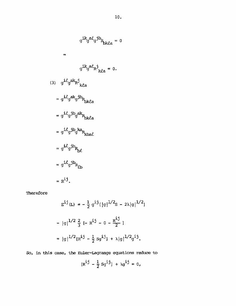
So, in this case, the Ner-Lagrange e q u a t i o n s reduce ~ 1 i j i j

[Rij - 2 s g ] + hg = 0,

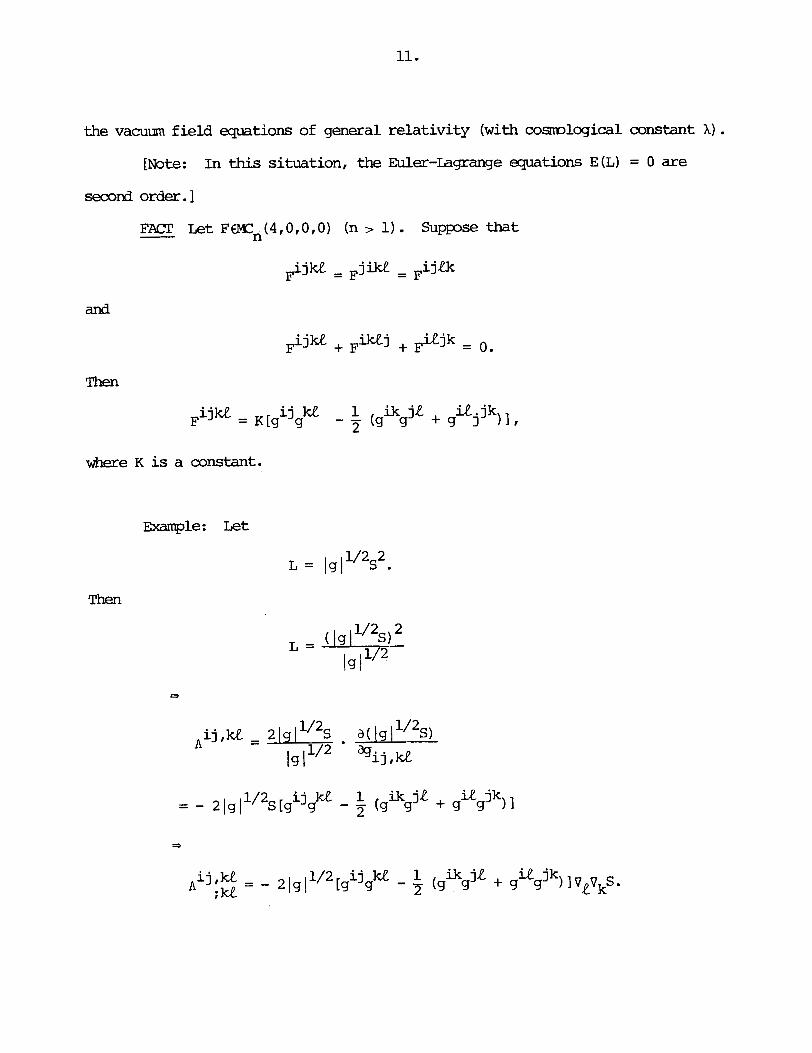
the vacuum f ie ld equations of general relat ivity (with cosmlogical constant 1).

[Note: In this situation, the Ner-Lagrange equations E(L) = 0 are

secorad order .I

FACI! - L e t FWn(4,0,0,0) (n 1). Suppose that

and

i jke + F ie jk = 0. F

Then

i j k e 1 i k j R ie . jk F ~ ~ ~ = K [ ~ g -I(g g + g 1 ) I .

where K is a constant.

Ekample: Let

Then

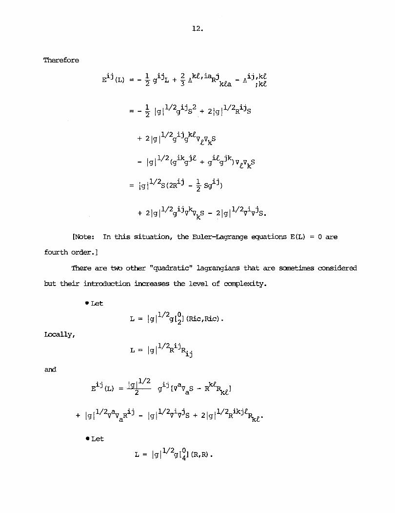
Therefore

i j E (L) = - 1 i j 2 z g L + - 3

[Note: In this situation, the Euler-Lagrange equations E(L) = 0 are

fourth order. 1

There are t m other "quadratic" lagrangians that are sametimes considered

but their introduction increases the level of cmplexity.

-lly,

and

Let

and . .

~~j (L) = I g 1 'I2 [4vatlaR1' - 2Pivjs1

Observation: W e have

FACT Take n = 4 -- then

Remrk: Take n > 3 and let

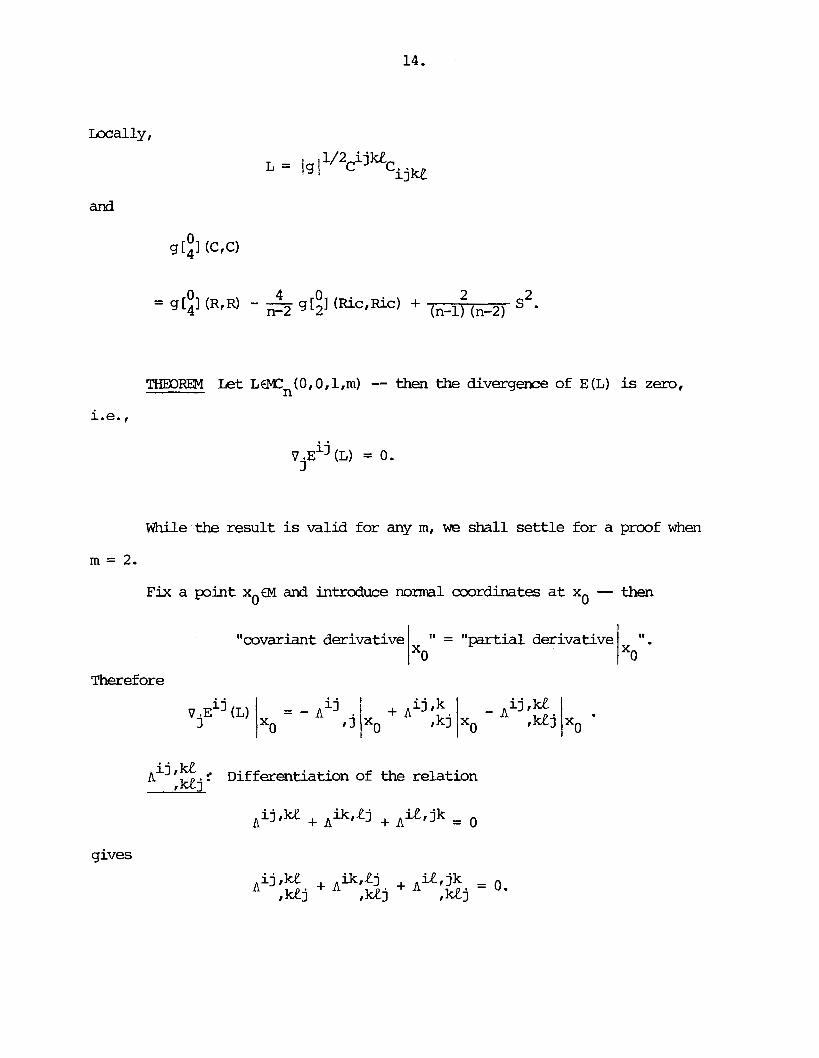
Lrx=ally,

and

THEORJ3M L e t L@Cn(O, 0, 1,m) -- then the divergence of E (L) is zero ,

While the result is valid for any m, we shall set t le for a proof when

m = 2.

Fix a p i n t x0€M and introduce normal coordinates a t xo - then

"covariant derivative " = "partial derivative

Therefore

A i j W Differentiation of the relation .kLi '

gives

But th is implies that

[Note: N o m l coordinates play no role in this argument.]

We shall now discuss the t m t e r m s on the RHS, beginning with

By definition,

B U ~ nijtk = 0, hence

Therefore

Since

or still,

- rid

is symetric in a & 1, it follows that

r3d. -

Rappel :

Thus at x 0'

and

Claim: We have

Therefore

Accordingly,

Next

Thus

Taking into account that ghrLk is spnetric i n L & k,

or still, since we are working at x 0'

It remins to explicate

Tb begin with,

So, in view of the fact that

at x we have, 0

But at xo,

Thus at xo,

Claim: We have

[Multiply the identity

Therefore

Recall now that

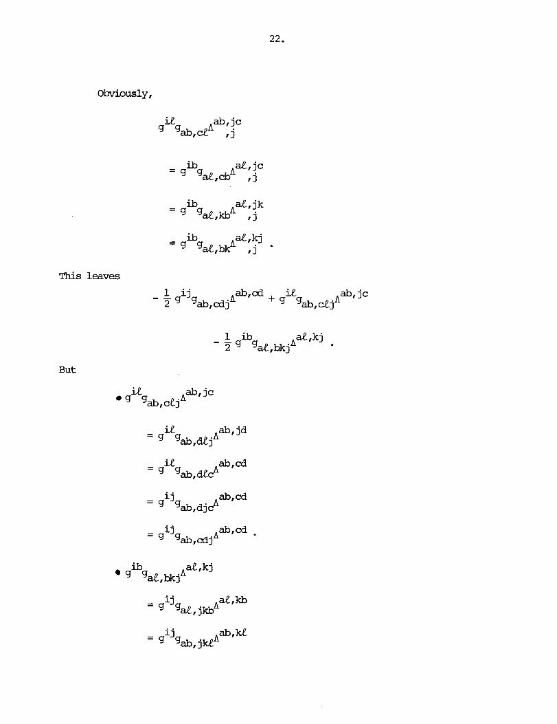
Obviously,

This leaves

But

It therefore

which completes the

follaws that

proof of the theorem.

Example: Take L = lgl -- then E(L) = lgl "2~', hence

# div G = 0 *d iv G = 0.

Thus the vanishing of the divergence of the Einstein tensor is just a particular

case of the theoran.

0 [Note: Officially, div GEVl(M), and

# div G# = g div G.

In fact,

# i ik (g div G) = g (div G)

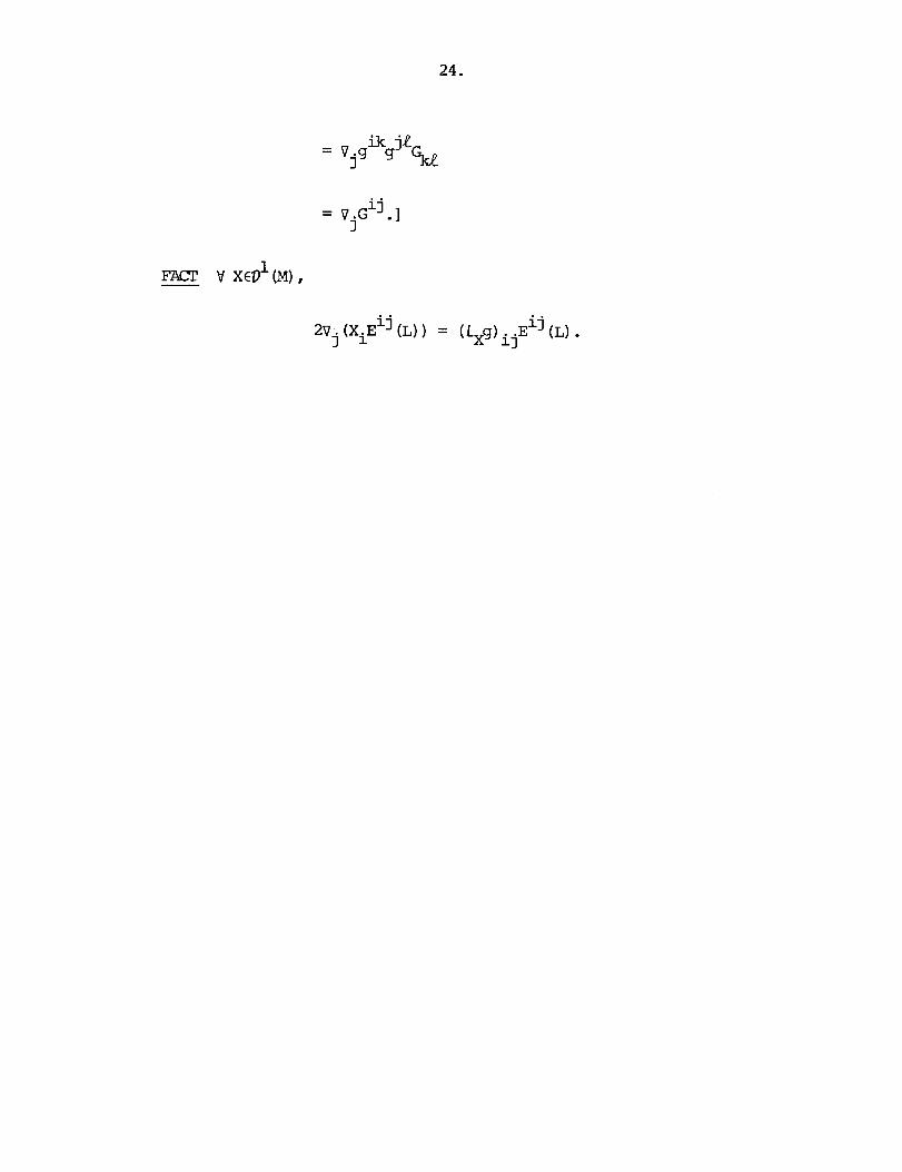
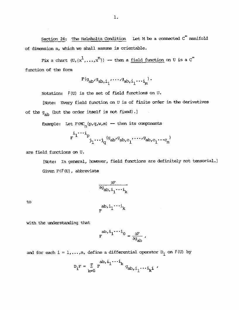
Section 24: The Helmholtz Codition L e t M be a connect& cm manifold

of dimension n, which we shall assum is orientable.

1 n Fix a chart (U,{x ,..., x } ) -- then a field function on U is a cm

function of the form

Notation: F(U) is the set of field functions on U.

[Note: Every field function on U is of f in i te order i n the derivatives

of the g* (but the order i tself is not fixed).]

Example: L e t F€Kn(p,q,w,m) -- then its cc~nponents

i . ..i F I j, . . . j q ' ~ ~ ~ ~ ~ , c l ~ * * * ~ ~ ~ , c ~ . . . c m 1

are field functions on U.

[Note: In general, however, f ield functions are definitely not tensorial.]

Given F E F (U) , abbreviate

with the understamling that

ab,il-0-io F - aF --

agab I

and for each i = 1, ..., n, define a differential operator Di on F(U) by

ab, il- 0 %

DiF = F g a b , i l - . . v 1

k-0

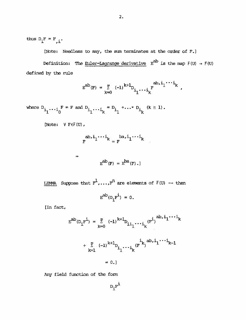
thus D.F = F 1 , i'

[Note: N e e d l e s s

Definition: The

defined by the rule

to say, the sum terminates a t the order of F.]

Ner-Lagrange derivative E~ is the map F (U) -+ F(U)

where D . F = F and Di - il*-*1 - D i o . . . ~ Di ( k z l ) .

0 1*-% 1 k

Sup~ose that F1, ...,I? are elements of F(u) -- then

[In fac t ,

= 0.1

Any f i e l d function of the form

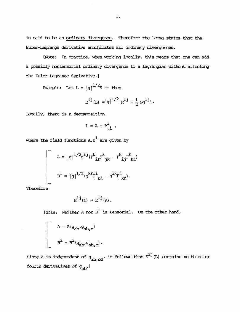
is said to be an ordinary divergence. Therefore the lama states that the

Euler-Lagrange derivative annihilates a l l ordinary divergences.

[Note: In practice, when working locally, this means that one can add

a possibly nontensorial ordinary divergence to a lagrangian w i t b u t affecting

the Ner-Lagrange derivative.]

Locally, there is a decamposition

where the f ie ld functions A , B ~ are given by

I - Theref ore

i j Eij (L) = E (A) . i

[Note: N e i t h e r A nor B is tensorial. On the other hand,

Since A is independent of g ab,cd'

it follows that Eij (L) contains no third or

fourth derivatives of gab. I

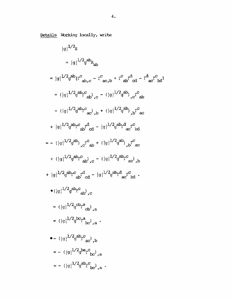
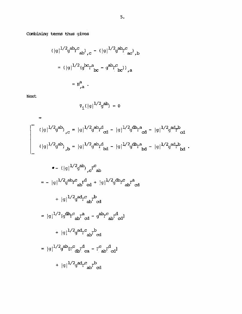
Combining terms thus gives

= B~ . fa

Next

1/2 ab vi(lgl g = 0

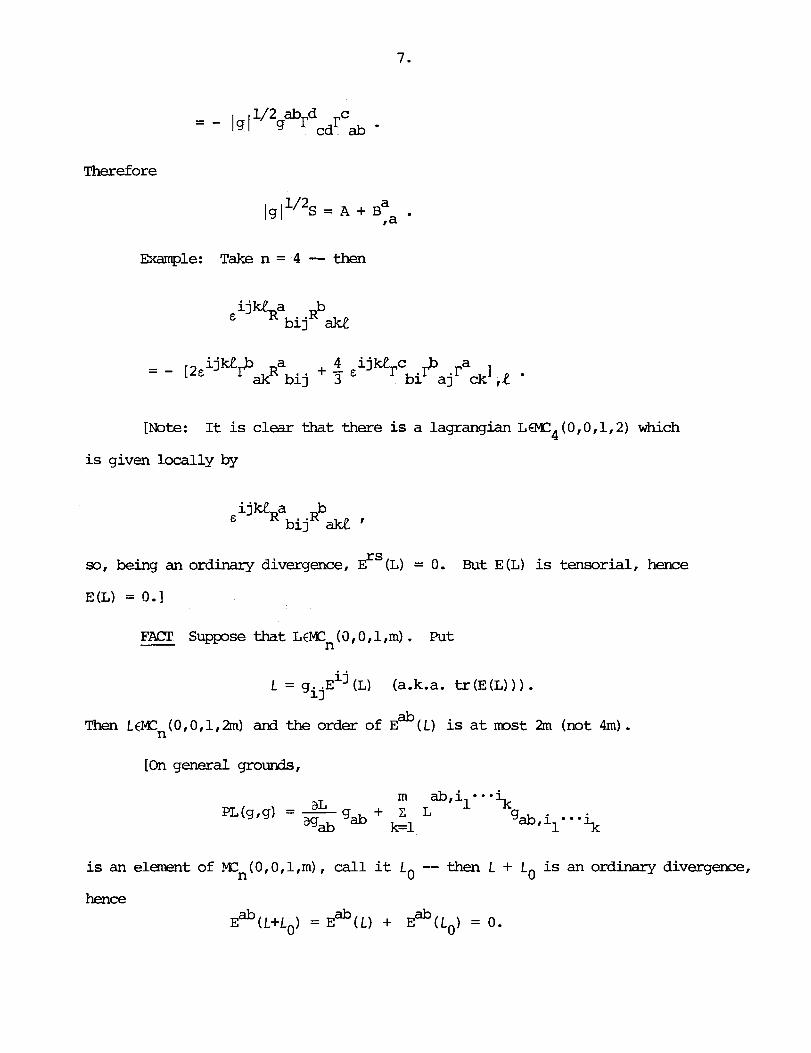
Therefore

Example: Take n = 4 -- then

E ij- b i j & ake

[Mte: It is clear that there is a lagrangian L ~ 4 ( 0 , 0 , 1 , 2 ) w h i c h

is given locally by

so, being an ordinary divergence, 8' (L) = 0. But E (L) is tensorial, hence

E(L) = 0.1

FACT Suppose that LcMCn(O,O,l,m). Put -

ab Then L c ~ ( O . 0 , l . h ) and the order of E ( L ) is a t mst 2m (not 4m).

[On general grounds,

is an el-t of En (0, 0, 1 .m) , ca l l it Lo -- then L + L is an ordinary divergence, 0

hence ab ab ab

E (L+LO) = E ( L ) + E (Lo) = 0.

ab ab But the order of E (Lo) is 5 a", thus the same holds for the order of E ( L ) .I

Ramrk: The notion of ordinary divergmce is local and involves partial

derivatives rather than covariant derivatives. In this connection, recall that

there is one important circumstance when the tsm notions coincide, viz. l e t

1 X € ~ - S D ~ ( M ) -- then

provided V is torsion free.

[Note: Put

xi E

j 1 . dx A ... A dx Jn-I "x = (n-l)! i j l -o -~n- l

or still,

n i+l i 1 *i n % = Z (-1) Xdx A ... Adx A ...dx. i=l

Then

mtation: Given FWU) and k L 1, put

where D. F = F. %+lo

. . -1 ab

[Note: Extend this to k = 0 by the agreement E

LIWJIA W e have

ab, il- a 'b ' , i l0**\ E (F)) + E ~ ~ ( F ) = 0.

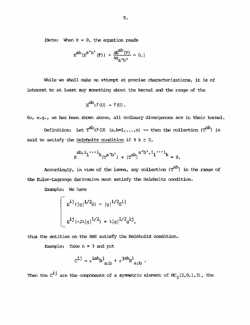
[Note: When k = 0, the equation reads

While we shall make no attempt a t precise characterizations, it is of

interest to a t least say sawthing about the kernel and the range of the

So, e.g., a s has been sbwn above, a l l ordinary divergences are i n their kernel.

ab Definition: L e t @€F(u) (a,bl. . . . ,n) -- then the collection {T 1 is

said to satisfy the Hehdmltz aondition i f V k 5 0,

ab, il* arb ' , il E

"'=k = 0.

ab Accordingly, in view of the lama, any collection {T ) in the range of

the Euler-Lagrange derivative must satisfy the Helmholtz condition.

Example: W e have

thus the ent i t ies on the RHS satisfy the Helmholtz andit ion.

Fxample: Take n = 3 and put

Then the cij are the compnents of a symnetric elenent of M33(2,0,1,3), the

Cotton tensor. W e have

In addition, it can be checked by ac~nputation that the Cotton tensor sat isf ies

the Helmholtz condition, although it w i l l be seen in the next section that there

does not exist a lagrangian

such t h a t

Nevertheless, there are f ie ld functions F such that Eij (F) = ciJ , one such being

F = - a k & 1 j i j b i E IT r iar jk,L + r iar jkr

Product Fule Let F,GEF(U) -- then

In particular:

ab Suppse that {T ) is a collection which sa t i s f ies the H e l m h o l t z condition - then

Notation: Given a f ie ld function F, let

W e have

Therefore

ab a'b' E (galblT = - - -

[Note : In general,

Tb see this, let E: be the Ner-Lagrange derivative per t2g -- then

ab 2 'b' Et (t galblTa2

t

On the other hand,

ab 'b' (@atbl@2 C

1 ab 2 a'b' ) = - t E (t gasb1T 2

t

Section 25: Applications of H a m g e n e i t y Let M be a connected cm

manifold of dimension n, which we shall assume is orientable.

Definition: L e t FEF(U) -- then F is said to be ~ e n e o u s of degree x

i f V t > 0 ,

For the record,

1- R i j ~ is ~ e n e o u s of degree 1

R is homDgeneous of degree 0 jc

ik j'% is hamogeneous of degree -1. - g i j u

[Mte: 1 g 1 is hamgenems of degree M2.1

ab LEMMA L e t T WU) be hrsmogeneous of degree x # -1 (arb = 1 ,..., n).

ab Assume: The collection {T ) sat isf ies the Helmholtz condition -- then

T* = E~~ (L) ,

where 1 L = - - a'b'

x+l ga'b'T

[ I n f a c t ,

= 2 (x+l) t 2x+lTab

But

ab a'b' E ( tgalb,T 2 = -

t

t2n+l$b 'b' 1 cgaIbJa ) = - 2 2(x+l) t 2x+lyab

ab a'b' E (galblT ) = - ab

(x+l)T .I

1/2Gi j E'xanq?le: Take n = 4 -- then Igl is horcogeneous o f degree 0 and,

as can be checked by computation, the c o l l e c t i o n { I g 1 'I2Gij 1 satisfies the

Helmbltz condit ion. Therefore

in agreement with the general theory.

m l e : Take n = 3 and let

Then the collection {c~'} satisfies the Helmholtz condition. Still, cij is

hmgeneous of degree -1, thus the foregoing construction is not applicable.

Ranark: Let AEM=n(2,0,1,m) (n > 1) be hormgeneous of degree -1 -- then it can be shown thatm a 3 if n is odd and m 5 n if n is even.

Symbol Pushing In the literature, one will find the following assertion.

ab Suppose that {T ) is a collection which satisfies the Helmbolt2 condition -- then

where

1 'bl L = - lo 2tga1b1~a2 dt. t

[Formally,

ab = T .

However there is a tacit assumption, namely that

And this is not true in general. I

-i 1 Let F€:n(p.qlw,m). Take x = - x (t > 0) -- then t

Specialize to the

hrxrogeneous of degree x,

il- -i casewhenq = 0, w = 0 -- then if F is

we have

or still, in view of the Replacement Theoran,

Classification i .. .i

0 If 2x+p = 0, then F is a function of gab alone.

i ...i 8 I£ 2x+p is positive, then F I p=o.

i ...i If 2x+p is negative and m t an integer, then F = 0.

If 2x+p = -2,-3,..., then F is a plymmial in the G~~~ l"*%

RePnark: If FEMCn(pIO,w,m) is hmgeneous of degree x , then

1g l Y I / % ~ ~ n ( p , ~ , l , m )

n is hmgeneous of degree x - (T)w. Therefore the structure of F can be ascertained

from the structure of 1 g 1 -1%.

Ll3Wl If n > 1 is odd and if L€M2n(0,0,1,m) is ~ e n e o u s of degree 0,

t h e n L = 0.

Example: The preceding 1- breaks down i f n is even. For instance,

is a second order lagrangian which is harrogeneous of degree 0, as is

FACT Suppse that L€MZn(0,O,1,2) is homqeneous of degree 0 -- then -

i j g. .E (L) = 0. 11

[Recall that

i j E (L) = - , i j - , i j M

;kt

But here

Notation: Given a f ie ld function F I let

Example: L e t LWn(O,O,l,m) -- then

Application: Supp3se that L ~ n ( O , O , l , m ) is hmru>geneous of degree 0 --

then E (L) Wn (2,0 , l , 2m) is hamgeneous of degree -1.

[In fact, Lt = L, hence

L =tZ. r t l

The re fo re

E(L Ltl = ~ ( t % ) = t n ~ (L) . On the other hand,

2 t E (L) = E (L)

1/t2

Example: Take n = 4 -- then L = 19 1 li2.S2 is homgeneous of degree 0, hence

is hamgeneous of degree -1.

UWMA Let L€M2n(0,0,1,m), where n > 1 is odd. Ass=: E(L) # 0 -- then

E(L) can m t be h g e n e o u s of degree -1.

[If E (L) w e r e hom3geneous of degree -1, then the relation

E (L) = tn-% 1/t2

reduces to

hence

But

where

is homgeneous of degree 0:

2 1 dn L ' ( s g) = l i m - ( - - L (s2g))

t+ 0 n! dtn [ t l

= L' (g) . Therefore, since n > 1 is odd,

L' = 0 = E ( L ' ) = 0 j E ( L ) = 0,

a con t r ad ic t ion . 1

By way of a corollary, there does not exist a l a g r a n g i a n

such that

Ei j (L) = cij

RBwk: L e t A€P.Cn(2,O,1,m) -- then in order that A = E(L) for SOE

l ag rang ian L, it is necessary t h a t Aij = Aji & 17 . A ~ ' = 0. I n addition, the 3

oollection {A~') rhst s a t i s f y the Helrhholtz condition. But , as the Cotimn

tensor shaws, these requirements are not suff icient .

FACT - L e t A m n (2, O , l t r n ) . Supwse that the collection {Ai'] s a t i s f i e s

the Helmholtz condition -- then

. . [Note: It is not assumed that Aij = A", thus the condition appears to

be asymnetric. S t i l l ,

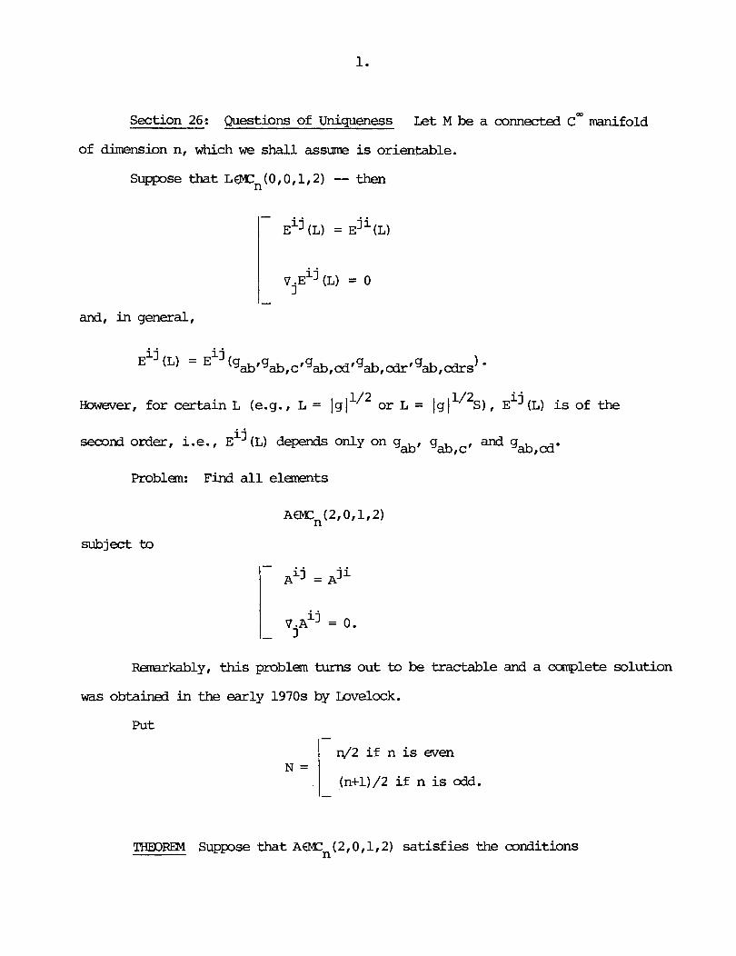
Section 26 : Questions of Unigtleness L e t M be a connected cW manifold

of dimmion n, which we shall assunre is orientable.

Suppose that LWn(0,0,1,2) -- then

- ji ~~j (L) = E (L)

i j V.E (L) = 0

and, in general,

However, for certain L (e.g., L = lg11/2 or L = l g ~ ~ ' ~ ~ ) , E ~ ' ( L ) is of the

i j second order, i.e., E (L) depends only on gab, gab,cf an.' gab,cd*

Problem: Find a l l elements

sub j ect to

Remarkably, t h i s problem turns out to be tractable and a conp?lete solution

was obtained i n the early 1970s by ~ v l o c k .

Put

THEOREM Suppse that AWn(2,0,1,2) sat isf ies the conditions

N =

- n/2 i f n is even

(n+1) /2 i f n is odd. -

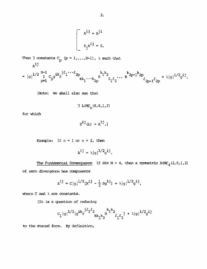
[Note: W e shall also see that

for which

Example: If n = 1 or n = 2, then

The Fundamental Conseguence If dim M = 4, then a symnetric AW4(2,0,1,2)

of zero divergence has ccxnpnents

where C and h are constants.

[It is a question of reducing

to the stated form. By definition,

And

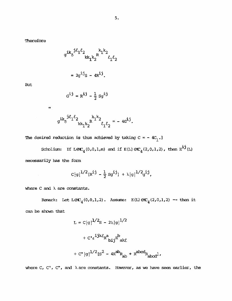
Therefore

But

The desired reduction is thus achieved by taking C = - 4Cl.]

Sd-nlium: If L€MC4(0,0,1,rn) and if E(L)€MC4(2,0,1,2), then E ~ ~ ( L )

necessarily has the form

where C and X are constants.

Ramrk: L e t L~4(0,0,1,2). Assume: E(L) ~4(2,0,1,2) -- then it

can be sbwn that

+ C'E i j v Rb bij ake

where C, C', C", and Xare constants. However, as we have seen earlier, the

terms multiplying C' and C" are annihilated by the Euler-Lagrange derivative,

hence per prediction, make rn contribution to the Euler-Lagrange expression

[Wte: The analysis that gives the structure of Aij when dim M = 4

applies verbatim when dim M = 3. On the other hand, there is a simplification

since the only L ~ j ( 0 , 0 , 1 , 2 ) for which E(L) ~ j ( 2 , 0 , 1 , 2 ) are the

Example: If n = 5 or n = 6, then

where C, Dl and X are constants.

W e shall now turn to the proof of the theoran. So let

subject to

Put

Identities

N.B. We have

a(vjAij) 1 i t ; a b , r ~ + ~ i s ; a b , t r + ~ i r ; a b ~ ~ t ~ . = 7 (A

rst

Identities

- A it:ab,rs + Ais;ab,tr + Air:ab,st =

'A it;ab,rs = Ars;abtit

Therefore

A it:ab,rs - Ait;rs,ab -

ab;rs, it = A

ab; it,rs = A

= 0.

Notation: For p = 1,2, ..., write

ab; ili2 i3i4; . . - ; i A 4 ~ - 3 ~ 4 ~ 2 1 i4p1i4p

[Note: This

Special Case

prescription defines an element of M2n(2+4p,0,1,2).]

Take p = 2 -- then

ab; il - i Properties of A 4~

(2) It is synrraetric wder the interchange of ab and i2k-li2k (k = 1,...,2p).

(3) It Satisfies the cyclic identity involving any three of the four

indices (ab) (i2k-li2k) (k = 1,. . . ,2p) .

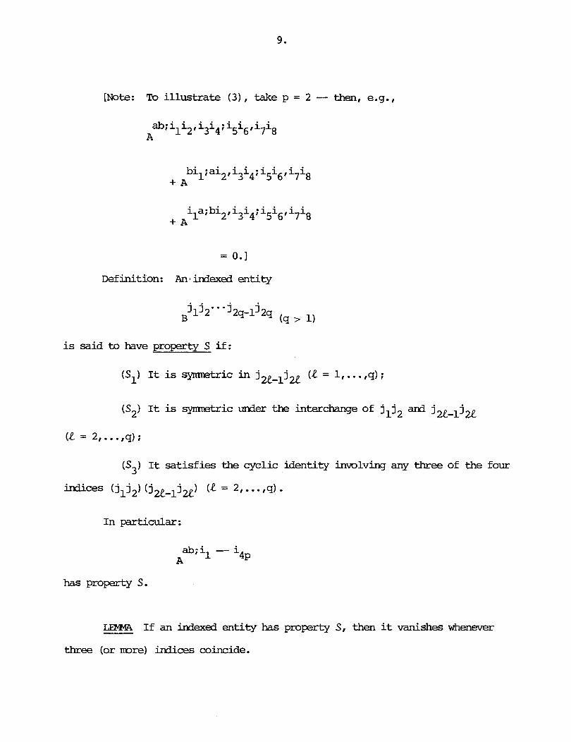
[Note : To i l lus t ra te (3) , take p = 2 -- then, e.g.,

= 0.1

Definition: Anlindexed entity

is said to have property S i f :

(S ) rt is symetric i n jXm1jX (e = l,.. ..q) ; 1

(S2) It is symnetric under the interchange of jl j dnd j - j Ze

ce = 2, ..., q);

(S3) It sat isf ies the cyclic identity involving any three of the four

indices (jlj2) (j2e-ljX) (l = 2, -. . .q) - In particular:

has property S.

LEMW If an indexed entity has property S, then it vanishes whaever

three (or mre) indices coincide.

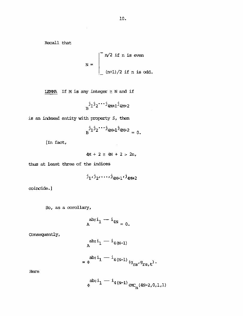
R e c a l l that

- n/2 if n is even

- (n+1) /2 if n is odd.

is an indexed entity with property S, then

[In fact,

4M + 2 r 4N + 2 > 2n,

thus a t least three of the indices

coincide. 1

SO, a s a corollary,

ab; il - i A

4N = 0.

ab; il - i A

4 (N-1)

H e r e

has property S. But, thanks to the Independence Theorem,

Therefore

ab; il - i A 4 (N-2)

Rappel: We have

where

Put

Then

2 ab; il - i - - - - + 4 (N-1) 3 j kit ++* I

where the metric concomitant

2 ab; il - i p'=q,*+-* 3 4 (N-1) rjkie

is a t mst a function of gr, and grSttr hence is a function of grs alone. Nau

i t e ra te the procedure ... . Sumnary: W e have

H e r e , the C are constants, P

is syrrmetric, thus has the form

114 lU2gab

for some constant 1.

It ra ins to explicate the

ab; il - i 4P

ab LEMMA Fix p:l I p 5 N-1. Dmote by S (n,4p) the subspace of

PCn(2+4p,0,1,0) consisting of tbose entities with property S -- then ab dim S (n,4p) = 1.

Notation: Put

Maintaining the assumption that 1 5 p r N-1, define

ab; il - i D 4P

i i i i 1 2 3 4 i x D . . .D 4p3i4p2i4pli4p

j lj 2s1s2 jzP1 j 2p s 2p-ls2l3 '

Then

ab; il - i D 4 p ~ ~ a b (n, 4p) .

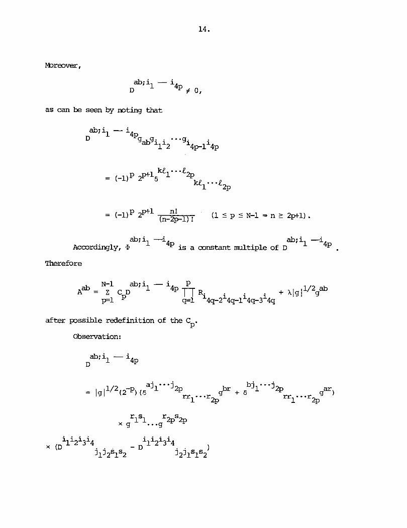
as can be seen by noting that

ab; il -i ab;il -i Accordingly, % 4P is a constant multiple of D 4~

Therefore

after pssible redefinition of the C P -

Observation:

ab; il - i D 4~

i i i i i i i i x - D 1 2 3 4

jlj 2s1s2 j 21 p1s2 )

To exploit this, mte that

Now bring in

and write

Thus, after adjusting the constants, we conclude tha t

But

So, m u l o obvious notational changes, the proof of the theoran is coimplete.

Remrk: The expression

. . is a polynomial of degree N-1 i n the R ab cd. Therefore, i f A~' is linear in the

second derivatives of the gab, then Cp = 0 for p > 1, hence the 21ij must have

the form

clg

Rappel: Let

Then

Then

To begin with

f ram which

Starda~~d manipulations involving the Bianchi identities then imply that

Matters thus reduce to consideration of

or still, to consideration of

the claim being that this expression is equal to j

But

Therefore

Ranark: L e t A F M C ~ ( 2,0,1,3) be sym~letric and divergence free -- then

where C, c, and X are constants. But, as w e kmw, there does not exist a lagrangian

L W 3 ( 0 , 0 , l ,m)

i j such that ~~j (L) = C .

Given p 2 1, put

Then

R e a l i t y Check Take p = 1 - then

and

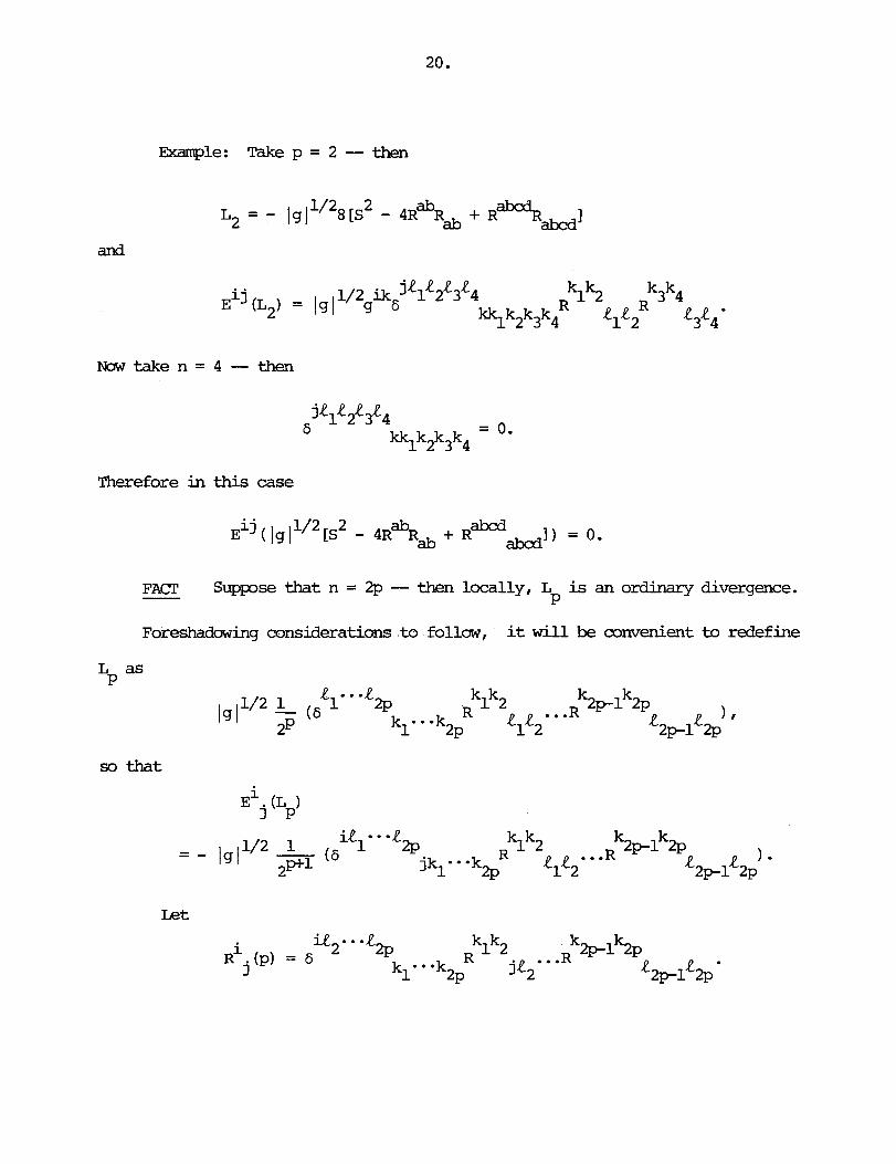
Example: Take p = 2 -- then

and

Therefore in th i s case

FACT Suppose that n = 2p -- then locally, L is an ordinary divergence. P

Foreshadowing mnsidaations to follow, it w i l l be convenient to redefine

L as P

so that

Let

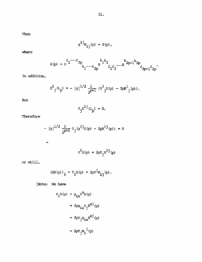
Then

where

In addition,

But

Therefore

vis(p) = 2 p ~ ~ ~ ~ j (p)

or still,

[Note: We have

= 2pV . R. j (p) 3 1

jb = 2pV jg Rib@)

b j = 2pg V.R. (p) lb

= 2phib(p)

j = 2pV Ri (p) = 1

Remark: The higher order version of Ric is Ric(p) :

R i ~ ( p ) ~ ~ = R. . (p). 13

Ric (p) is symetric and

t.r Ric (p) = S (p) , 9

the higher order version of the scalar curvature.

Therefore

i E .(L) = - lg

3 1

[Note: The relation

reduces to

in agreemnt with the earlier theory.]

Section 27: Globalization L e t M be a connected cm manifold of dimmsion

n, which we shall take to be orientable with orientation EL. Fix a s e m i r i d a n

structure g on M.

Rappel: Given x0€M, there exists a conneded open set UcM containing xo

and vector f ie lds E,, ..., En on U such that V x<U,

Because of this, there is no real loss of generality i n assuming outright

that the orthonormal frame bundle IM(g) is t r iv ia l .

[Note : -9s a matter of convenience, in what follows we shall work with

oriented orthonormal frames but a l l the results in this section can be formulated

in terms of an arbitrary oriented frame. I

So f i x an oriented or thonoml frame E = {E1,...,E }. Denoting by n

= { o f . . . , an} its associated mframe, put

- - 1 E .

3n eil. . i (n-p)! ~ - - - i p j p l - - - j n (I) Ip1n ... n o .

P

Then

il* .i 8 P = , ... E i B i . (no sum)

j-1 p l---lp

Observation: View the 8 . as the oomp~nents of an element 8 of p P

A"-P(M;T;(M) ) . L e t P be the metric connection -- then

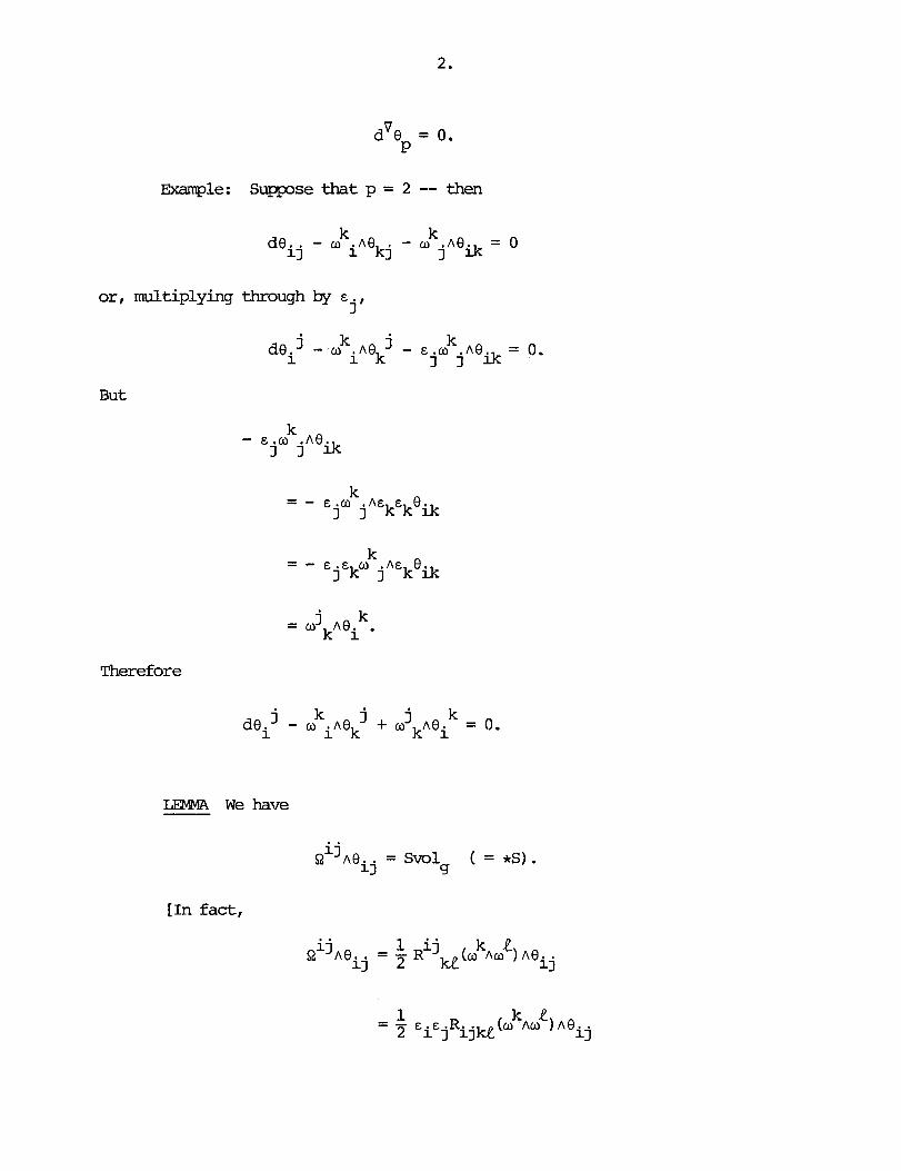
Example: Suppse that p = 2 -- then

or, multiplying through by E j

But

- E ok At3 j j i k

- - - E ok A& E e j j k k i k

= - c E ok A& e j k j k i k

Therefore

LEMMA We have

[In fact,

1 = - R k l i j 2 i jke (a AO ) A * (a ~o

1 = - R g(o k l i j ha ,o AO )vol 2 i jke 4

On the other hand,

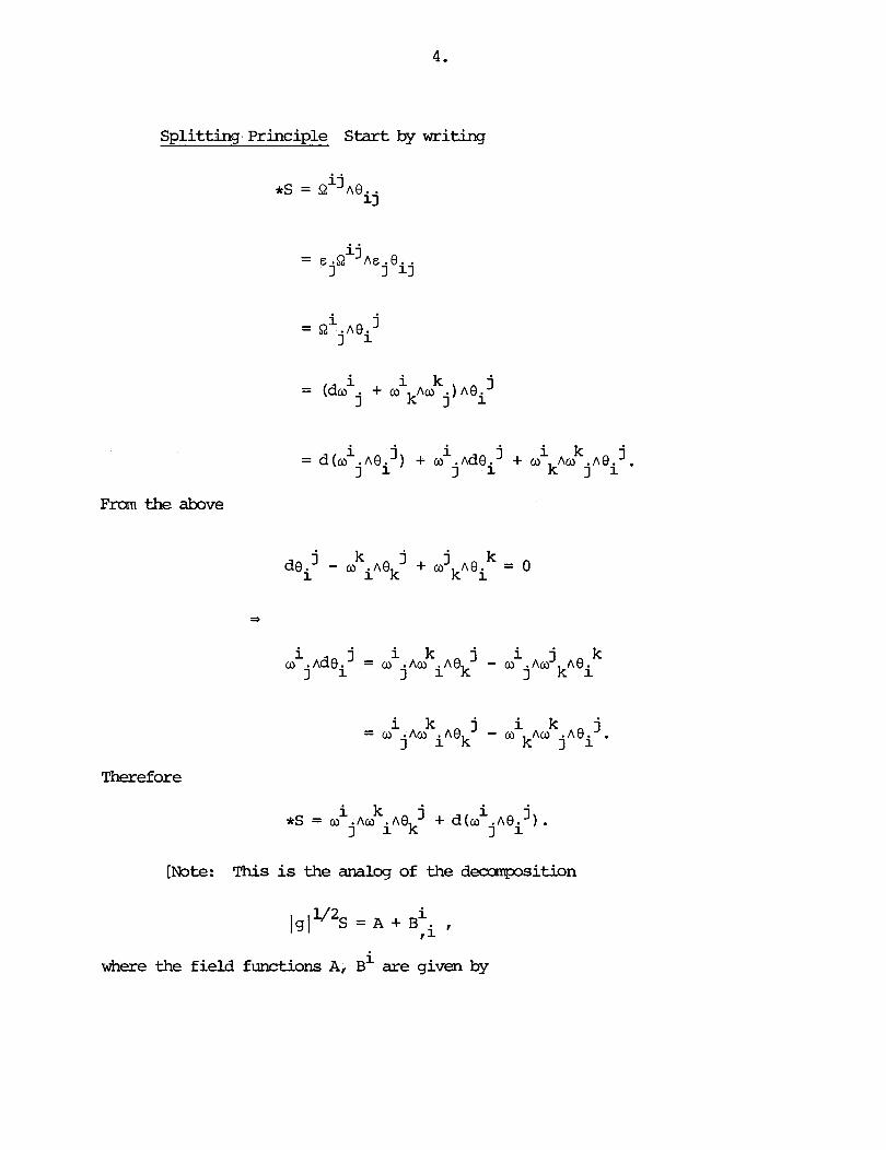
Splitting Principle S t a r t by writing

i j *' = '

Fram the above

Therefore

[Note: This is the analog of the decmposition

where the field functions A, B~ are given by

LEMNA We have

i j 1 i j - (do no ) A * ( d o . A o . ) + 2 (do no.)~*(do no.). 3 1 1 3

[First

i j = (do.. + w nok ) h ( o A o 1 13 ik j

But

i j d(w. . A * ( o A w ) )

1 3

i j i j = d w . . A * ( o AW ) - a. ~ d * ( o AO )

11 1j

i j = do. .A* (w Am )

1 3

i a j i a - o. A [- o A* (o no ) - oj A* (o no ) 1 1j a a

i j i a j = &. 1 3 . A * k o no ) + 2wijnw a ~ * ( o A w )

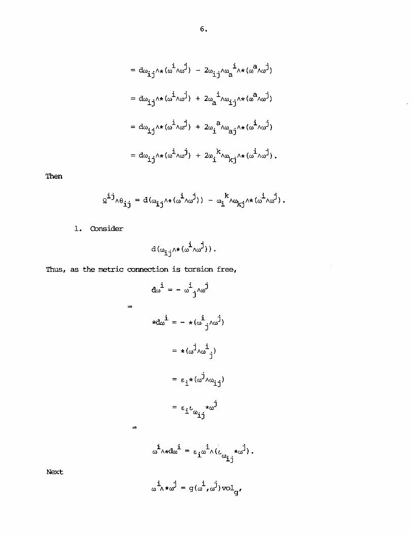
i j i a j = dw. ./\*(a A w ) + 2w A w . . A * ( @ A w )

1 3 a 11

i j i j = do. . A t ( o A o ) + 2 w . k A % j A * ( o A o ) . 13 1

1. Consider

Thus, as the metric connection is torsion free,

Next

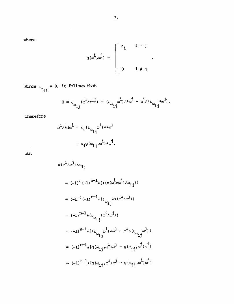
Since L~ = O f it follows that ii

Therefore

But

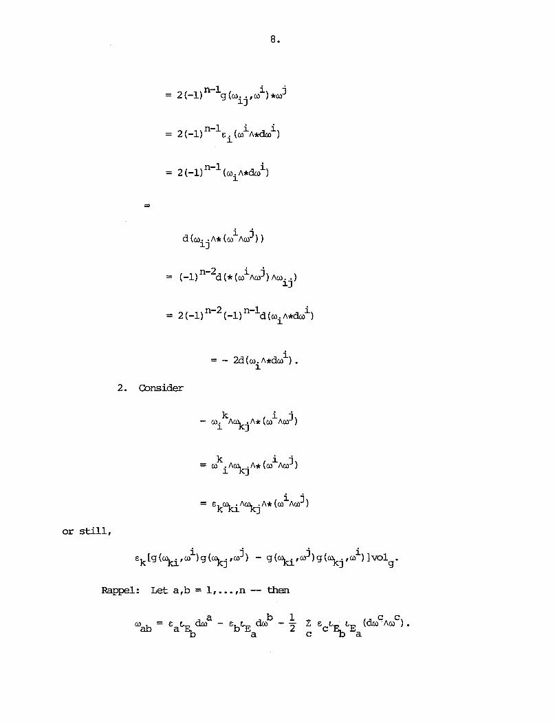
2. Consider

or still,

Rappel: L e t a,b = 1, ..., n -- then

Analogously

Write

Then

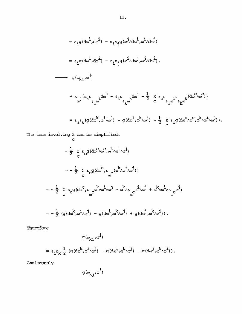
i i i j j i = gig(& #do ) - E . E . g ( W Ada ,W A d o ) .

1 1

k i j j z &,g(do c c k i j n o ,o Aw Ano ) ) . = E . E ( g ( d ~ ,o AW ) - g(dw I W Aw ) - - 1 k c

The term involving Z can be simplified: C

c c k i j Z c c g ( d w A w ,o A m A o ) - "i C

- - - - 1 c k i j Z ccg(do , L (o c W

- - - - c k i j k i j k i j Z E g(do ,L w Am A w - w Ac o A o + o A w Ac o ) c C C C C o W 0

1 k i j j k i #2: - - g ( d w ,w A o ) g ( & ,a no ) . 4

1 k i j i k j #3: - g(da ,w no ) g ( d w ,a Aw ) .

1 j k i k j i #7: - - g ( d w ,w Aw ) g ( d o ,w Aw ) .

4

1 j k i j k i 118: ? i g ( h ,w AO ) g ( d w ,o AO ) .

Six of the terms cancel out:

- E E E x ( # l + #8) = 0 k i j

'kEiEj x ( # 2 + #7) = 0

E.g.: Take #8 and w r i t e

1 k j i k j i = E E E g(do ,a Ao )g(dw ,a Aw ) j i k a

- - - 1 k i j k j i E E E - g(do ,o )g(dw ,a Aw 1, j i k 4

which is - E E E x (#I). Observe too that k i j

E E E X (#4) = E E E X (#5). k i j k i j

It remains to discuss

E E E x (#4 + #5 + #6). k i j

To this end, note that

- 1 k j i k j - - - E E . E . ~ ( w ,L id^ )g(dw ,w Aw ) 2 k 1 3 w

- 1 i k j i k j - - - E E . E .g(o Aw ,dm )g(dw ,a Aw ) 2 k l ]

1 k i j i k j = - E E.E.g(o h.l ,do )g(dw ,w Aw ) 2 k 1 3

= E E E x (#4 + 15) + ckcicj x (#6) k i j

+ ckeic x ((86).

he l a s t step is to study #6. In terms of the objects of anholonamity, there

is an expansion

i = E E.C k j kj*

On the other hand,

1 g(aoitaoi) = - & E.(C i 2 2 k j kj).

Combining these facts then gives

1 .skcicj x (#6) = - 4 E k 1 1 E.E.(c~ kj l 2

1 - - ( T 6.1 1. (- 2 E k j E.(ci kj 12)

1 i i = - E g ( b ,do 1, 2 i

fran which we conclude that

j i Ekg(%,a )g(%jr~

- - - - i i j j i i E . E . ~ ( ~ o Aa ,do ) + cig(da ,da 1.

2 1 7

i j 1 i = - (do Am )~*(do.Aw.) + 2 (do ~o~)~*(dojno.).

1 1 7

A l l the terms appearing in the statement of the lerrana are ~ G W accounted for.]

Put

L = vol 0 g '

Given p 2 1, put

Then

L €A%. P

[Note: These definitions are i n d e m e n t of the choice of E.]

Exarrqples :

* L1 = Svol g -

LEMMA We have

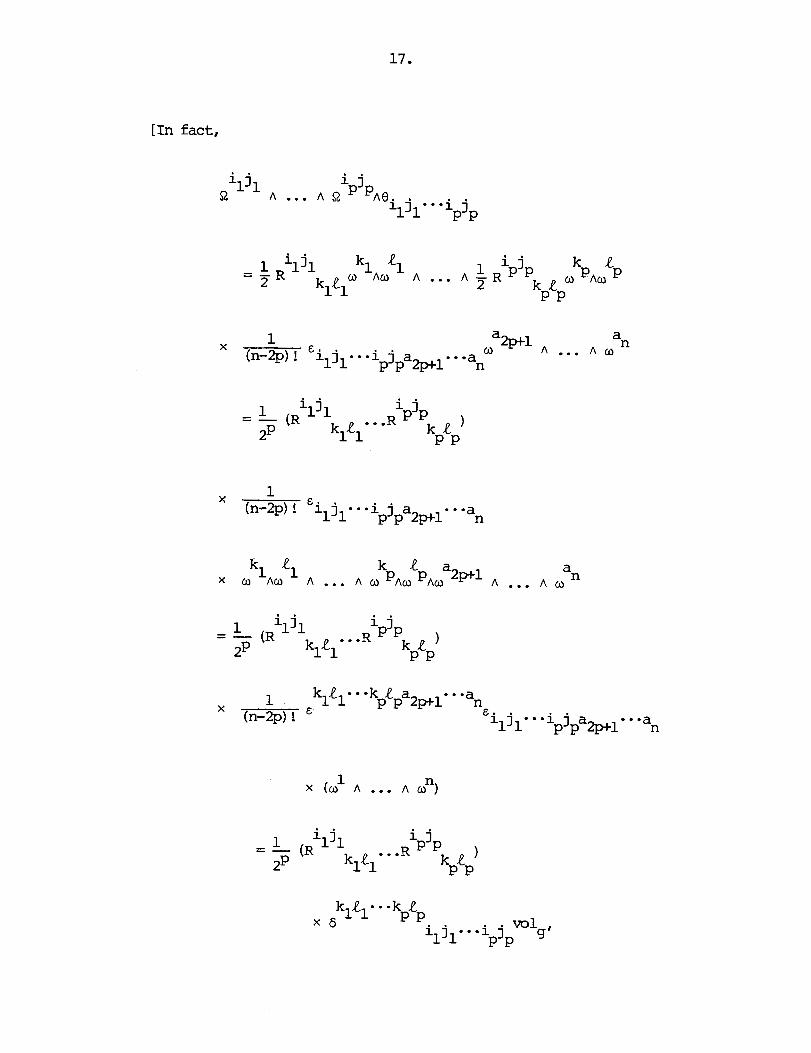
[In fact,

which, upon relabling, is equivalent to the assertion.]

Remark: If M is compact and riemmnian and i f n = 2p, then by the

Gauss-Bonnet theoren,

-,

the LHS being the N e r characteristic of M.

[Note: Take n = 2 -- then p = 1 and Ll = SVol .hbrewer, the scalar '

curvature S is twice the sectional curvature K and the Gauss-Bonnet theorm in

this case says that

I X (M) = JM Kv01 .I

4

FACT Suppose that n = 2p. Fix i E { l , ..., n) and l e t -

where

and

Then

[Note: Therefore L (n = 2p) is exact i f the orthomrmal frame bundle P

M(g) is trivial, hence is locally exact in general.]

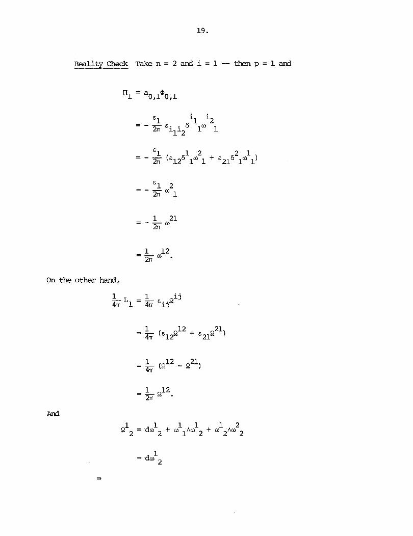
Reality Check Take n = 2 and i = 1 -- then p = 1 and

On the other hand,

And

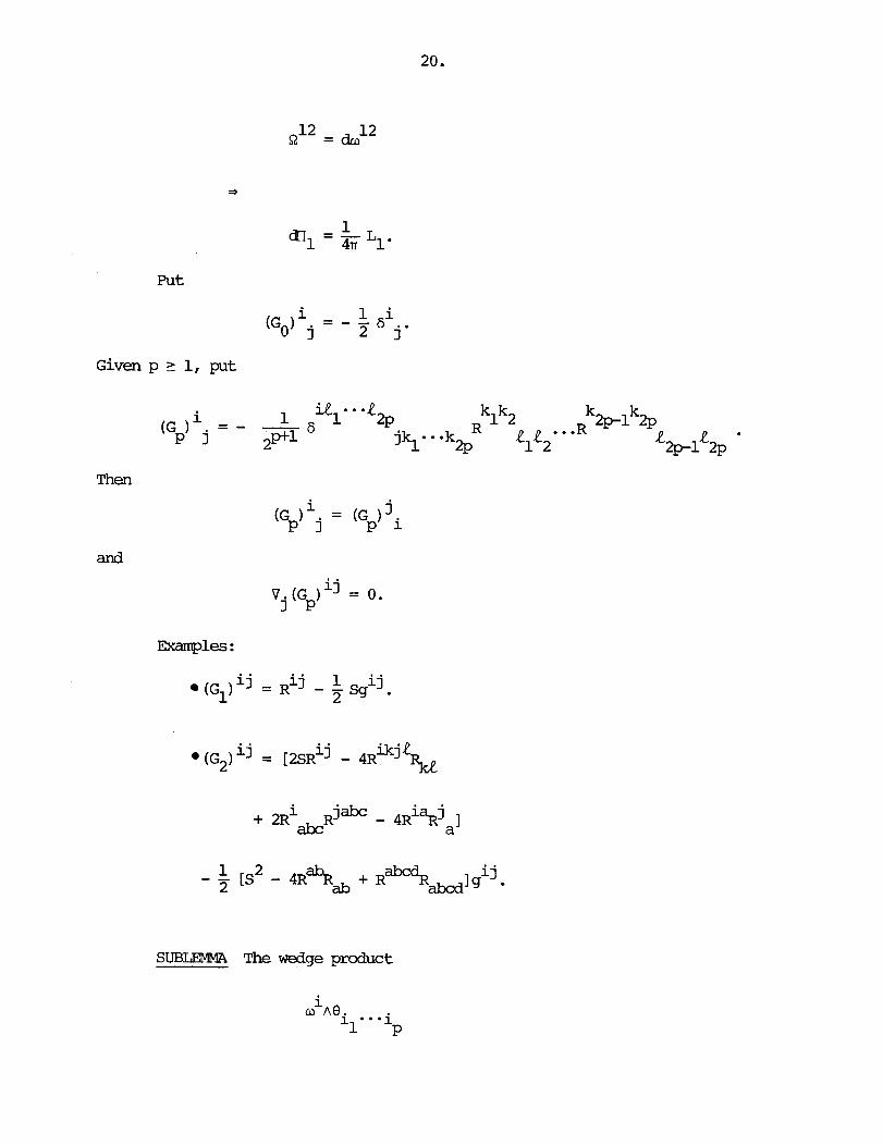
G i v e n p r 1, put

men

and

SUBLEMW The wedge product

can be written as

[Recall that

where

Therefore

P r i = (-11' C (-1) 6 . . .ci ci ..- Ei ei i ir 1

. . .1 r==l r-1 r+l p 1 r - 1 'p

But 6\aivci = 0 i f ir # i while G ~ ~ ~ E ~ _ ~ ~ = E . E = 1 i f i = i. Therefore 1 i r

Example: Suppose that p = 1 -- then

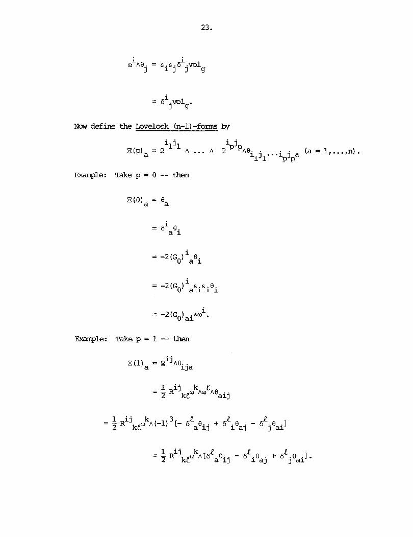
Now define the Imelock (n-1)-forms by

m l e : Take p = 0 -- then

Emmple: Take p = 1 -- then

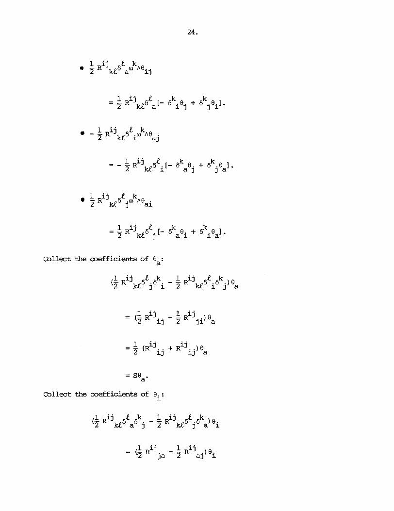
Collect the coefficients of Ba:

Collect the coefficients of Bi:

Collect the coefficients of 8 - j '

Therefore

UWMA W e have

SupFose that n = 4p (p = 1,2,. . . ) . Given (alI.. , aW) . put

and set

where

Then

[Note: The n_K are called Pontryagin forms. In view of the definition, -

their n e is precisely P(n/4) (P the partition function) .I

Emmples:

a n = 4:

a b i!(2) = Q bAQ a'

n = 8 :

Observation: is closed, i.e.,

[This follows f m the fact that

i k j. k = 0.1 deij + w kAQ - 8 kAw

j j

Thus Example: Consider aab~9 a '

a b a a c b a ,AQ a = (dm + co c~~ b) AP a

c b = dwa nab + wa Aw A8 b a c b a

a b a b a c b = d(o AQ ) + CO bAdS1 a + bA8 a b a c

a c b + w CAw bAS2 a

b a A a b ) - ma A w AaC = d h b a b c a

b + ma A$ A Q ~ ~ + 2 haC A9 a. b a c b

But

a c b w c A ~ bAS2 a

Therefore

a b b c aa A Q ~ = A& ) - ma AU nn a b a b a b c

b c a b c = d (aa A (daba + w nw a) ) - w bh cAQ b c a

b b c = d[wabAdw a + wa Aw Aw a] b c

b c - wa A o A 8 a b c

a b a b c = d[o b~do a + o Aw c A ~ b

a b c - w bAw c d

A (dm a + dAw a

a b = d [w b ~ d w a + a bAw b ~ o F ] c a

c a b a b c d - do Aw bh - bAw cA" a a

a b c = d[aa Adab + Aw b a b c

b a b c d - ha A> - CO bAW CAO d A a a c b a

a b c = d lwabAdwba + w AU ~w b c

a b c b c d a Aw A* A o - do b Aw c a - b c d a '

1 b c - d(wa Aw ch a) 3 b

1 b c 3 b c

b a a b a - do no AZ + docah c] = 7j [do b~~ cAo a c b a

- - b a b c a c b - [ha no AoCa - do Aw Ao f do Ao bAo 3 b c c a c

1 b c = - [& nob A$ - doa nob + doabAw Ao

3 b c a b a c c

b c a b c = 1 [ h a nub noC 4- ba AO A03 a + dw cAo 3 b c a b c b

a b c = do Ao Aw a. b c

Theref ore

a b a b a bAa a = d(w bAdo a)

a b c 1 a b c + d(w bAw a) - 3 d(w bAw a)

a b c d - w bAO CAw dAw a

a b 2 a b c = d[w b A d O + - (w Ao ch a 3 b

a b c d - b ~ o cAo d A ~ a.

However the last t e r m vanishes, so

a b a b 2 a b c a b ~ a a = d[m b ~ d m a + 5 (a bAw cAo a) 1.

[Note: To check that

a b c d Aw Aw dAw a = 0' Oh c

write

a b c d o bAw cAw d k o a

- - - a b c I w b A ~ d A ~ a'

FACT W e have

51 = dC*I -2k

where

[Note: To explain the notation, recall that

1 is an element of A (M;gt(n,R)) - - (here, of course, v is the metric connection).

Accordingly I

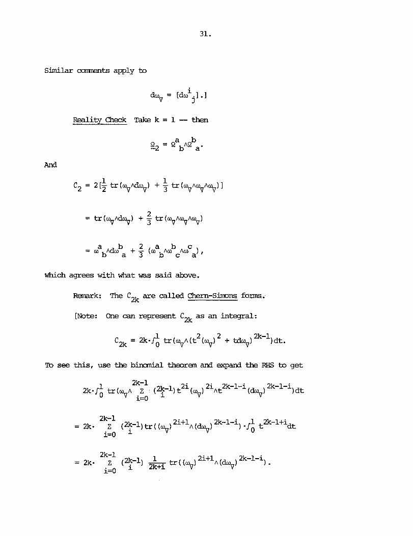
Similar cmnents apply to

Realitv Check

And

Take k = 1 -- then

which agrees w i t h what was said above.

R8nark: The C2 are called olern-Simons forms.

[ N o t e : One can represent C2 as an integral:

1 2 2 '2k = 2 - l o tr(gA(t (g) + tduv) at.

To see this, use the birmmial theorem and expand the FWS to get

E.g.: Take k = 1 and put

2 a (t) = t d w p + t (OAO). v V v Then

n = jJ tr (av (t) A Q ~ (t) ) dt -2 Odt

= dtr(ovAdov + (o V V V Am Ao 1 ) -1

Since = 0, it follows that

[Note: Suppose t h a t i c j - then the difference

thus is exact. I

Section 28: Functional Derivatives Let U and V be linear spaces equipped

with a bilinear functional < , >:U x V -t - R.

Definition: < , > is nondegenerate if

Suppose that< , > is nondegenerate -- then the arrows

1- V+U* (v+ < rv>

are one-to-one (but, in general, are not onto) .

- 64 (4) Let 4:U + R -- then the functional derivative -of 4 w.r.t. u€U 6u

is the unique element of V (if it exists) such that \d uv€U,

- w (9) Let $:V -r R -- then the functional derivative =of C w.r.t. VW

is the unique elemnt of U (if it exists) such that V v'W,

FWnark: Functional derivatives give rise to maps

Example: Take U = V = - Rn and let c , >:I?" - x - Rn + - R be the usual inner

product: < x,y = x-y. Suppose that f:Rn - + - R is a cm function -- then V X , ~ E R ~ , -

by the rule

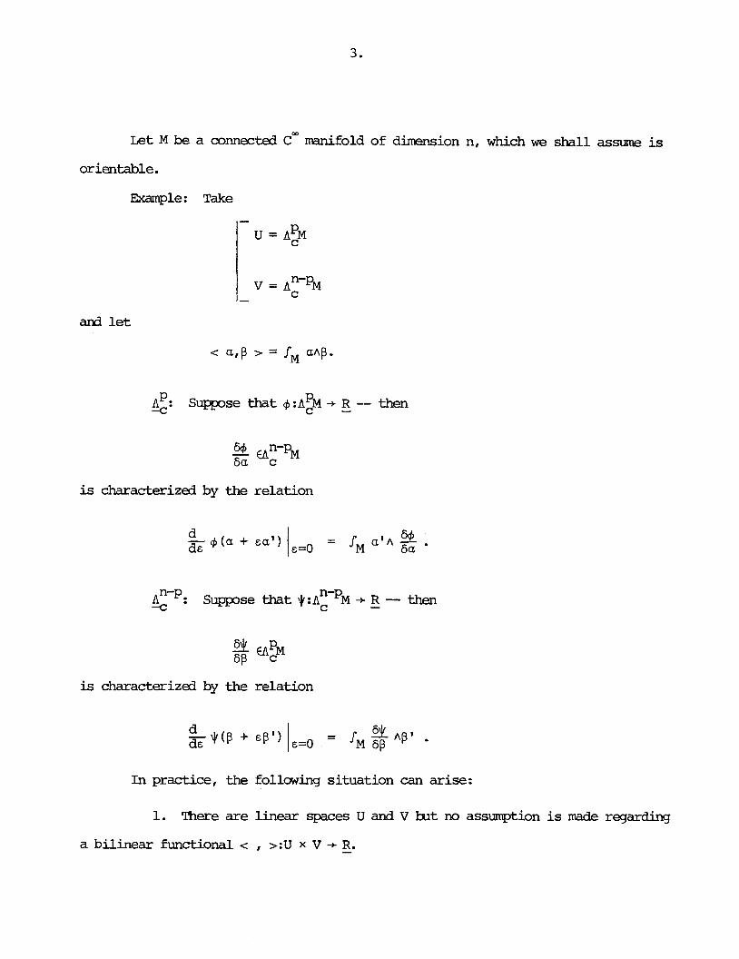
Let M be a connected cm manifold of dimension n, which we shall assume is

orientable.

Eample: Take

and l e t

is characterized by the relation

is characterized by the relation

In practice, the following situation can arise:

1. There are linear spaces U and V k t no assumption is made regarding

a bilinear functional c , >:U x V -+ R. -

2. There is a linear subspace UccU and a nondegenerate bilinear

functional c , >:U x V -t R. C -

3. There is a subset UOcU such that V uO€UO & H uc€UC, u0 + EU €U c 0

provided E is sufficiently small.

Under these conditions, i f 4:U0 + R, - then it makes sense to consider

W e shall rmw consider a realization of this setup.

W r i t e C: (M) for sec (Lden) , a d u l e over cm (M) -- then for any vector

bundle E -t M, there is an arrm of evaluation

ev: sec (E) x sec (E* 8 Lden) + C: (M) .

Let

Put

2 1 SP T*M -

Denote by S (M) the set of ccanpactly supported elements of S2(M) -- then there 2,c

- be the second symnetric power of

TM -- then

- T*M

is a nodegenerate bilinear functional

viz . < s , X @ r p > = JM X(s)dmq .

Scholium: The preceding considerations are realized by taking

Example: Let

be a lagrangian of the form

where ~ ~ ~ ( 0 , 0 , 0 , 2 ) (e.g. 1g1~'~~). Then, by definition,

and we have

PL(g,h) = - ev(h,E(L)) + div X(g,h) . H e r e

X (g,h) Esec (TM @J Lden)

is ccanpactly supported. If M is compact, then

exists and

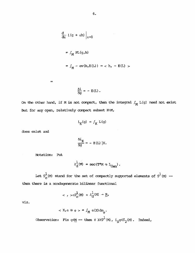
On the other hand, i f M is not compact, then the integral IM L(g) need not exist

but for any open, relatively ccanpact subset KcM,

does exist and

Notation: Put

1 Ad (MI = sec (T*M @ Ldm) .

1 1 Let VC(M) stand for the set of compactly supported elments of V (MI -- then there is a nondegenerate bilinear functional

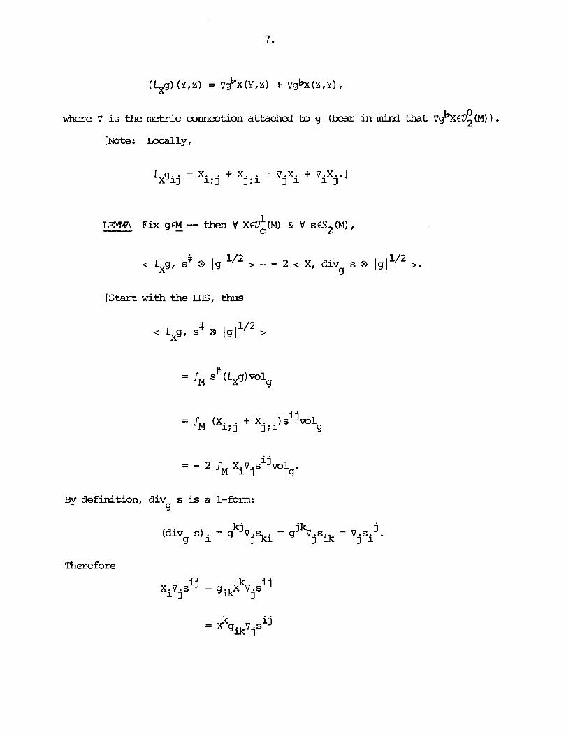
0 where v is the metric connection attached to g (bear i n mird that ~gbXC0~ (M) . [Note: Ixx:ally,

- Lxgij - xi; + X j i i = V.X. + ViXj.l

1 1

By definition, div s is a 1-form: g

k j - jk (div ~ ) ~ = g ~ ~ j ~ k i - 4 v j s i k = v . s j l i ' g

Therefore

= c X, div s 63 lg11'2 >.I 9

[Note: There is an integration by parts implicit in the passage from

i j 1, (Xi;j + X. . I S vo1 1; 1 9

to

ij - 2 1 X.V.s vo M 1 3 g '

In fact,

1 Claim: 3 YCDc (M) such that

To see this, observe that

has conrponents

Naw apply the contraction

Then

has compnents

and is ccsrrpactly supported. Consequently,

Each g€M - determines a IMP

# Thus write A = s 0 lg11/2 ( s € S 2 ( M ) ) and set

1/2 div A = d i v s @ 1st . 9 9

= s, A ( L ~ ~ )

1 Example: Suppse that XCD, (M) . Fix g € M - and def h e

by

Then

1 2 mample: Suppose that X E V ~ (MI . Fix A €Sd (M) a d define

# = JM s (L&-l)mlg

or still (cf . in£ ra) ,

Here

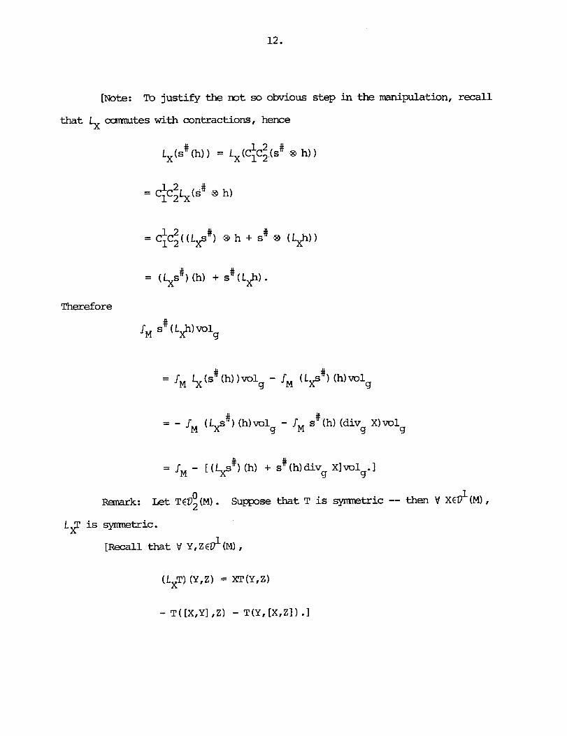
[Note: To justify the mt so obvious step in the manipulation, recall

that LX camutes w i t h contractions, hence

# 1 2 # L X ( s (h)) = LX(C1C2(s 8 h))

# # = - JM ( LXs ) (h) wlg - IM s (h) (div X) vol g 4

# = - I(*#) (h) + s (h)divg Xlvol .I 4

0 1 Ramrk: L& TCD2 (M) . Suppose that T is symEtric -- then 'd XCD (M) ,

L? is symnetric.

[Recall that \I Y . Z € D ~ ( M ) .

Notation: Le t g€M. -

G i v e n sB2 (MI , put

G i v e n s €S2 (M) , put

[Note:

(1) s * s € S 2 ( M ) . Proof:

= s S e

jl i*

( 2 ) tr (s*s) = [s,slg. Proof: 9

i j k = g s s i k j

Suppose given a function

defines a function

[Note: If M is ccgcrpact and if

w 2 then in the applications, - €Sd (M) exists, so @3

Examples :

(1) Put *(g) = lgy2 -- then

Therefore

provided M is capact.

[We have

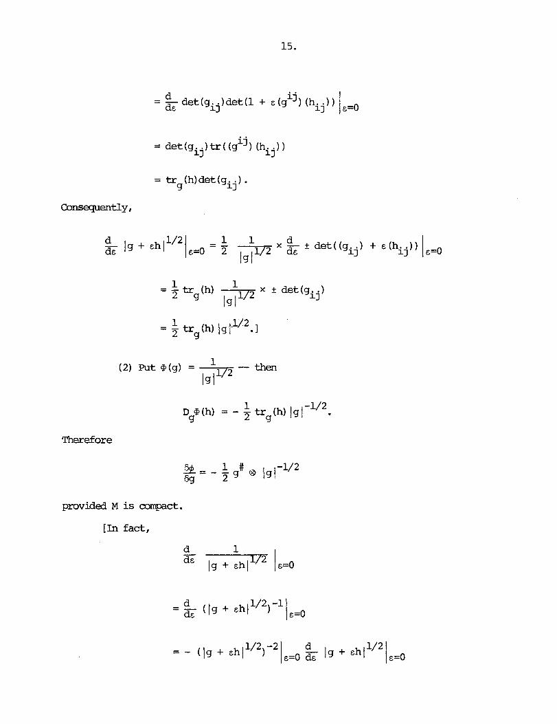
Therefore

provided M is compact.

[In fact,

Then

provided M is compact.

[To begin with ,

But

Accordingly,

(4) Fix s ES2 (M) and put

Then

Therefore

provided M is compact.

[Simply mte that

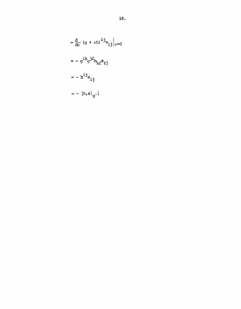
Section 29: Variational Principles L e t M be a connected cm manifold

of dimension n, which w e shall assume is orientable.

L e t

V:M - + con TM

be the m p that assigns to each g€M - its metric connection vg -- then

Locally,

k 1 ke (DgV (h) ) ij = g (VihLj + V , .h it - Vehij) r

which shows that D V(h) is synanetric in its covariant indices. 4

[Note: L e t $ (g + ~ h ) be the connection coefficients of V g + dl -- then i j

1 FACT Take h = LXg (XEDc (M) ) -- then

D V(Lxg) = 5 v g . 4

Example: Consider the interior derivative

6 :A% + crn(&l) , 9

so locally

Then

- - da ai' &=o

i j i j d = h v.a 3 i - g - ( ~ ? + ' ~ ~ ) l d.5 I i E=O

i j = h (Valij - g i j d

h 'ai, j - Th i j (9 + Eh) ak) la.O . . i j

= h (Valij + gl' & ?. 13 . (g + ah) /a=O\.

But

i j 1 kt = 9 2 g (vihRj + vjhie - v R h i j ) %'

In addition,

Therefore

Let IXijke(g + ah) be the curvature components of V g + &h

UMMA We have

Then

On the other

But

I - $st = ts'

so the equality of the tsm expressions is obvious. I

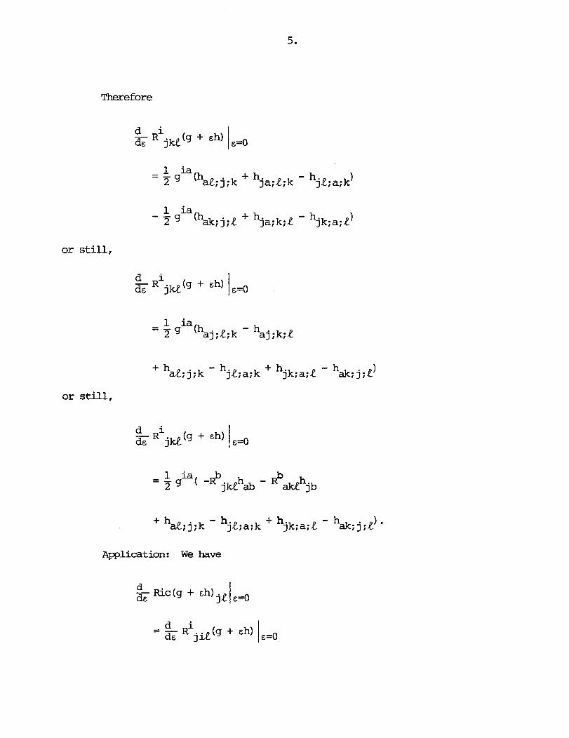
Therefore

d i - R (g + eh) 1 ds jke &=O

- 1 i a - - - h 2 j;k + hja;l;k jl;a;k 1

- 1 i a 3 g (hak ; j;l + hja;k;l - hjk;a;l 1

or still,

ds

- h - + &; j;i j t ; a ; i + hj i ;a ; t a i ; j ; ~ ) *

Hidden within this formula ( i tse l f perfectly respectable) are certain

conceptual features that are not imnediately apparent.

Notation:

* Given s ES2 (M) , define

R ( s ) ES2(M)

@ Given u,v€S2 (M) , define

by

Then

u*v + v*u€S2 (M) .

Definition: The Lichnerowicz laplacian is the map

k:S2(M) -+ S2(M)

defined by the prescription

[Note: Ix>cally,

FACT Suppose that g€M is an Einstein metric: - -

Then

divg 0 L+, = - hcon 0 div + a div g n g '

Given ~cA!M, put

thus locally,

LENVIA View Ric as a map

e c : M - -t S2 (M) . Then

1 = [kh + rdiv h - Htrg(h)l. g

[It is a question of conparing cc~nponents. For this purpose, start with

d (D Ric) (h) = - Ric (g + ~ h )

9 de

1 i a - - h - h 2 (haL: j ; i jL;a;i + h j i : a ; ~ a i ; j ; ~ )

Fi rs t

E=O

But

And

So rdiv h is accounted for. N e x t g

- ( A h) = - apl con j R jL;a;b

= - g141jL;a; if

which takes care of one of the t e r m s in (kh) jL. Finally

1 = ( -Htr (h) j tr g

thereby dispatching the hessian. What remains fmn ( ~ ~ h ) ~ ~ is

the claim being that this must equal

ia b g ( -R jiehab - R h ) a i l jb

= - gaq= jiehab

- - - ~~~h j t ab

- - - a b h R j t a b .

- g i q ~i j hjhaa

= - h t i j ab

- - - b a h R t j a b

= - a b h j L ab.

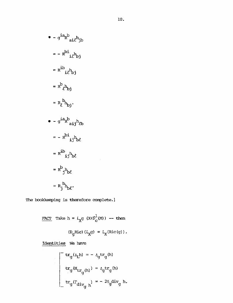
The bookkeeping is therefore ccarq?lete.l

Identities We have

Consider now

Special Case

SO, as a corollary,

where

[Note: Each of the terms involving V V h is a divergence. For exan~ple,

Example: Given an open, relatively compact subset KcM, put

Then an element g€M - is said to be critical if V K & V h€S (M) (spt hcK) , 2,c

d d 1 = 0. lK ~ ( g + ch) wlg + IK S(g) n l g + ,h

But

d ( = - I 1 S(g)trg(h)volg '-K S(g) zW\ + ch &=O 2 K

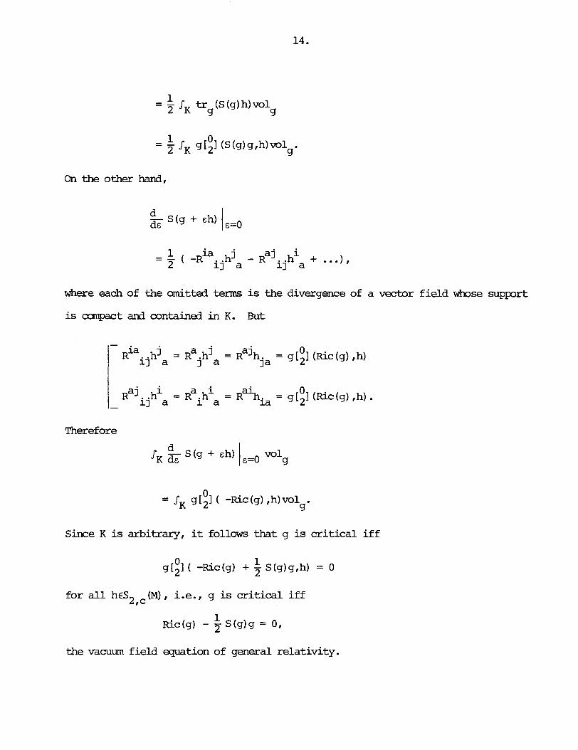
where each of the Oncitted t e r m s is the divergence of a vectDr field whose support

is compact and contained in K. But

Therefore

0 = IK gL21 ( -hc (g) ,h)vol

g '

Since K is arbitrary, it follows that g is cri t ical i f f

0 1 gL21 ( -Ric ( g ) + 2 S (g)g,h) = 0

for a l l h€S (M) , i .e. , g is crit ical i f f 2,c

1 Ric(g) - S(g)g = 0,

the vacuum field equation of general relativity.

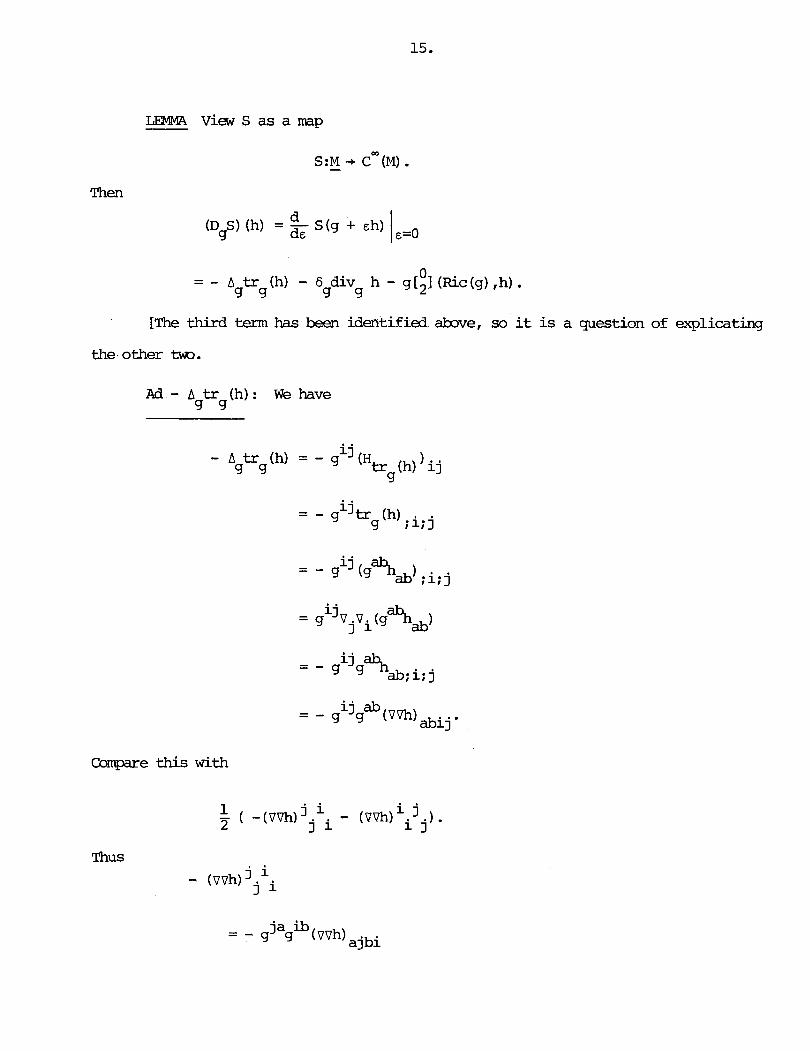
LENMA View S as a m p

Then

0 = - A tr (h) - 6 div h - g[*I (Ric (g) ,h) .

g g 53 4

[The third term has been identified a v e , so it is a question of explicating

the other tm.

Ad - A tr (h): W e have 53 g

Capare this with

Thus

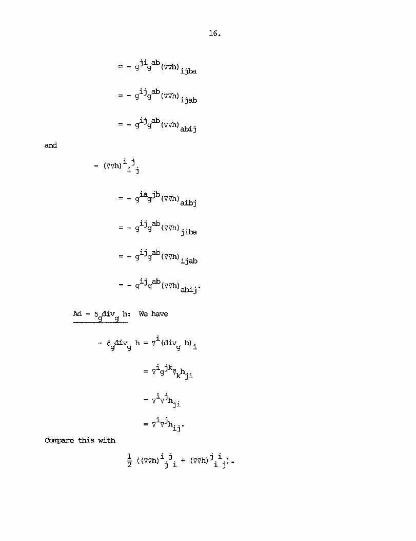
and

Ad - 6 div h: W e have g 9

i - 6 div h = v (div h)i g 53 9

- i jk - g Vkhji

i j = v v hji

i j = v v hij.

Compare this with

1 z ((vvh)ijji + (vvh)jiij I

Thus

and

Example: Take M caopact and let h = Ric (g) -- then trg (fit (g) ) = S (g)

and

1 div Ric ( g ) = -Z dS (g)

g

1 - 6 div Ric(g) = ( -6 dS(g)) g g g

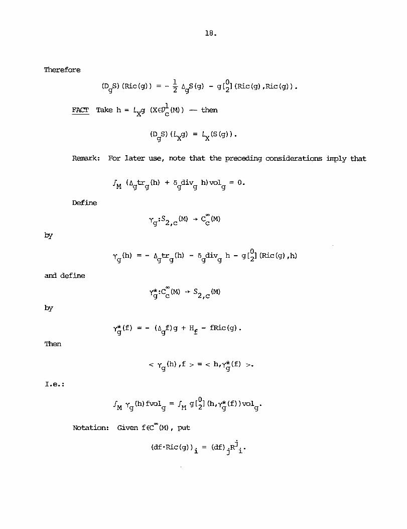
Remark:

Define

by

and define

by

Then

(DgS) (Lxgl = Lx(S(g)).

For later use, note that the preceding considerations imply that

S, (A tr (h) + 6 div h)vol = 0. 9 9 9 9 9

0 yg(h) = - A tr (h) - 6 div h - g[*1 (Ric(g) ,h)

9 9 9 9

~otation: Given f€cW (M) , p t

j (df*Ri~(g))~ = (df) jR i.

S- Let f ccrn(~) -- then

div H - dngf - df-Ric(g) = 0. 4 f

[By definition,

But, in view of the Weitzenboeck formula,

And

Suppose that y* (f) = 0, thus 9

- (A f ) g + Hf - fRic(g) = 0 4

and so, upon application of div 4 '

- d~ f + div H - df-fic(g) - fdiv Ric(g) = 0. 4 4 f 4

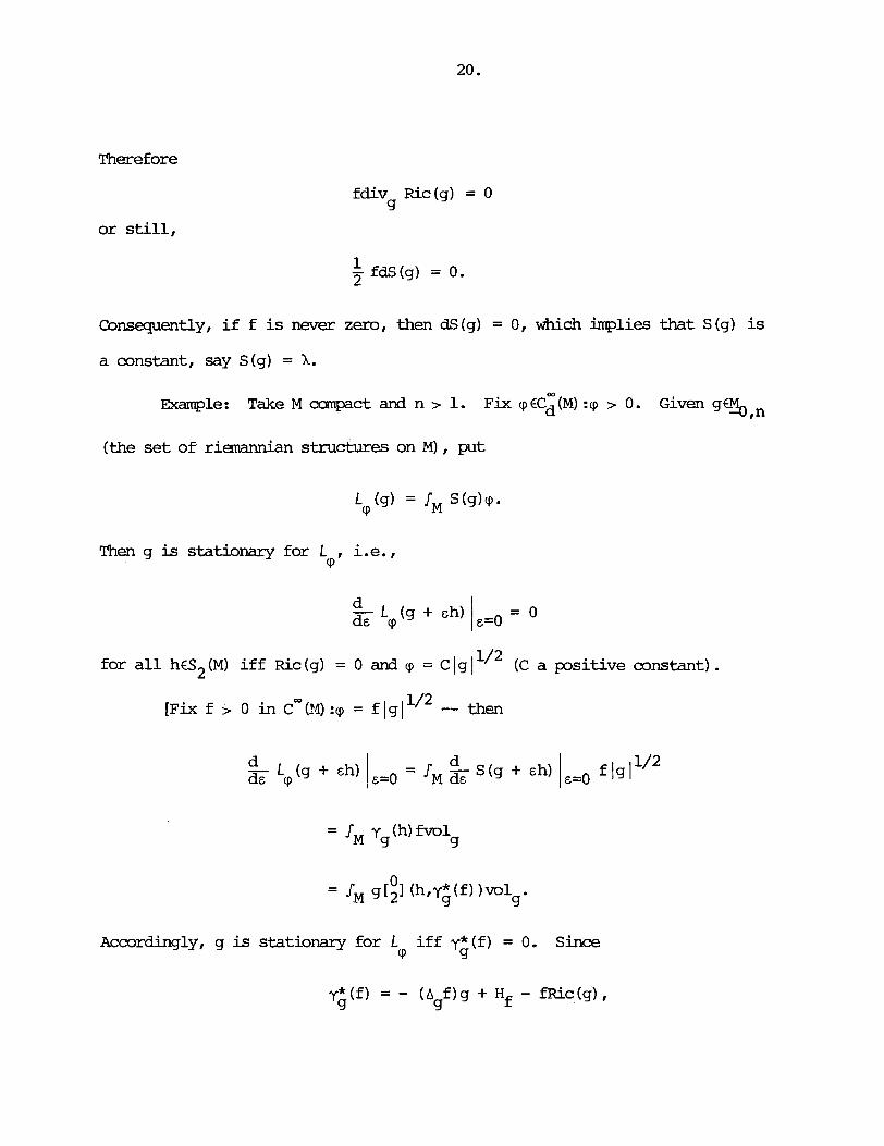
Therefore

fdiv Ric (g) = 0

or still,

Consequently, i f f is never zero, then dS (g) = 0, which implies that S (g) is

a constant, say S (g) = X.

Example: Take M c a p c t and n > 1. Fix cp€ci (M) :cp > 0. Given g% rn

(the se t of rimannian structures on M) , put

Then g is stationary for L , i.e., cP

g $, (g + Eh)

for a l l hcS2 (M) i f f Ric (g) = 0 and cp = C lg

= 0

1 'I2 (C a positive constant) .

[fix f > 0 in ~ ~ ( 1 4 ) :o = f 1 ~ 1 ~ ' ~ -- then

d d - ' (g + Eh) I E = O = fM '(9 + 'h) lgl 1/2

d& cp

= I Y (h) fvolg M

- - I, g121 0 (h,y;(f) )vol '

Accordingly, g is stationary for L i f f y* (f) = 0. Since cP g

yG(f) = - ( A f ) g + Hf - fRic(g), g

the conditions

are obviously sufficient. To see that they are also necessary, mte that

But

If X 7 0, then .fM fwl = 0, contradicting f 7 0. Therefore X = 0, hence f is g

harmnic :

And

Then

0 = y* (C) = - m c (g) g

=. Iiic(g) = 0.1

[Note: There may be m g a t which L is stationary. 1 cP

IXWN View Ein as a mp

1 = - [ A $ + T 2 + (6 div E)gl

d i v g g

[Note: Here

thus locally, - - 1 a hij - hij - 2 h agij. I

1 FACT Take h = Lxg (X€Dc(M)) -- then

It is sametimes necessary to consider second order issues, the dawnside

being that the computations can be involved.

Example: Put

Differentiate the identity

once w.r.t. e and then set E = 0 to get

div' Ein (g) + div (D Ein) (h) = 0. 9 h 9 9

Therefore

div (D in) (h) = 0 9 9

Differentiate the identity

twice w.r.t. E and then set E = 0 to get

div" Ein (g) + 2diviIh (DgEin) (h) + div in) (h,h) = 0. 9th 9 9

Therefore

div in) (h, h) = 0 9

if

[Note: Strictly speaking, div" should be denoted by div" gr h 9, (hrh) - I

Observation: L e t X be an infinitesimal iscawtry per g and suppose that

s tS2 (M) is divergence free (i . e. , div s = 0) . Define X. s by 9

j ( X * S ) ~ = x Sij.

Then

6 X - s = 0. g

[In fact,

i 6 X - s = - V (X-S) 4

i j = - v (X s . . )

17

But

V.X. + V.X. = 0 1 3 3 1

mlication: Suppose that

Then for any infinitesimal ismetry X per g,

2 6 X- (D Ein) (h,h) = 0. g g

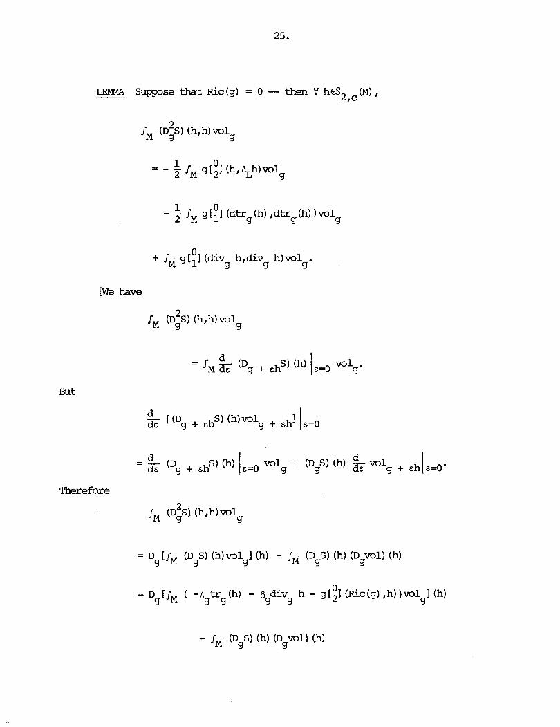
0 + .fM g[l] (div h,div h ) w l 9 9 9'

[We have

But

1 + - J ( A tr (h) + 6 div h ) t r (h)vol 2 M 4 4 4 4 4 4 '

The term

1 0 - - 2 I M g[,l (h,ApLh)VOlg

requires m further attention, hence can be set aside. Next

And

= JM (div h) (div h) ivol g g g

0 = & g[l] (div h,div h)vol 9 g 9 '

1 0 = - J gll] (div h.dtrg(h))wlg. 2 M 4

Thus these terms cancel out, leaving

or still,

Then

2 + I, S(g) ( D g w l ) (h,h).

Suppose now that g is a c r i t i ca l point: Ein(g) = 0 =, Ric(g) = 0 & S (g) = 0, thus

1 0 0 - - 2 M g (dtr (h) ,dtr (h) )vol + JM g[ll (div h,div h ) w l 4 4 4 4 4 4

+ $ g [ ; ] (h,h) + 26 div (h*h). 4 4

[Note: Here Vh*Vh stands for the cambination

Reality Check This amounts to calculating the integral

2 r, (DgS) (h,h)volg

2 directly £ran the expression for (D S) (h,h) provided by the lama and camparing

g

the result w i t h the formila obtained earlier (which was derived urader the assunption

that Ric(g) = 0).

[Note: If Ric (g) = 0, then

By definition,

= v v j v h k i j '

Therefore

Write

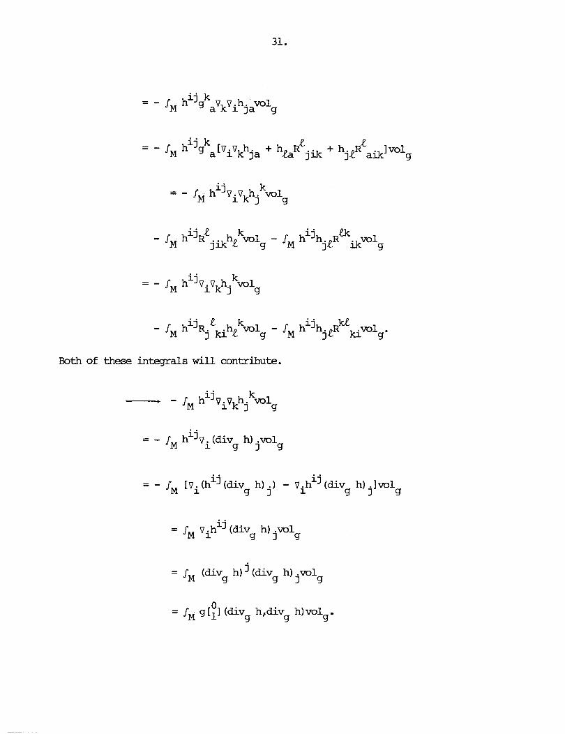
ij k = - J,h ViVkhj vo1

g

i j k ij kt - J, h ~~~~~h~ vo1 - I, h h j L ~ pig. g

Both of these integrals will contribute.

i j k - - JM h V.V h. vol 1 k 1 g

i j = - J, h vi(div h) .vol

9 1 4

ij i j = - JM [vi(h (div h) .) - Vih (div h) . lvol

9 3 9 1 g

= J v.hij(div h) .vol M 1 9 1 g

j = 1, (div h) (div h) .vol 4 9 1 4

0 = S, g[ll (div h,div h)vol

9 g 4

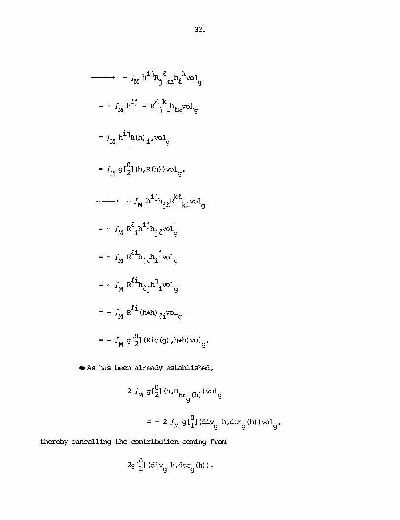
As has been already established,

0 JM g [2] (h,Ht, (h) )wlg 9

0 = - 2 JM gill (div h,dtr (h))wl

'3 g g

thereby cancelling the mntribution coming f m

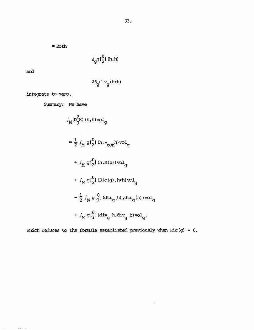
Both

and

integrate to zero.

Sum~lry: We have

0 + JM gill (div h,div h)wl 9 4 g '

which reduces to the f o d a established previously when Ric (g) = 0.

Section 30: Splittings Let !I be a oonnected cm manifold of dimmion n.

Assume: M is compact and orientable and n > 1.

Ekpip %(MI with the cm toplogy -- then &MI is a ~ r & h e t space. In 9

0 particular : V 2 (M) is a E'rkhet space, as is S (M) (being a closed subspace of

0 P2 (MI I . nbbreviate M to % -- then M is open in S2 (M) , hence is a ~ r & h e t

-O,n -0

manifold mdeled on S2 (M) . Given gE4. define

by

and define

by

# a* ( s ) = - 29 div s . 9 4

Then

2 o ( a ;x) :T M -+ Sym T*M 5 9 X X

of a is injective. g

[Given V€TxM, we have

1.e.: V = 0, hence a ( a ;x) is injective.] 5 9

By el l ip t ic theory, it then follows that there is an ortbgonal deacarrposition

S2(M) = Ran a @ K e r a*, FI Q

where both Ran a and K e r a* are closed subspaces of S2 (MI . 9 9

Consequently, every sES2(M) can be s p l i t into tm pieces:

s = s + h g . 0

H e r e div s = 0 and &g is unique in X up to infinitesimal imtr ies . 9 0

Mtation: Given x€$ ( M ) , put

[By definition,

j j = v V.X. + v Pixj 3 1

m i n g to vjvixj, write

£ram which the result. 1

[Note: This computation does mt use the assumption thatM is campact

and is valid for any g€M. - I

Application: Suppose that Ric (g) = 0 -- then

A tr k g + 6 div &g = 0. g g g g

[Consider A h k g : (3 g

Consider 6 div kg: 9 9

But

~a-1: Suplpse that Ric (g) = 0 -- then tl h€S2 (MI ,

Example: Suppose that Ric(g) = 0. Let h€S2(M):h = ho + k g (div h = 0) -- 9 0

then

(D Ric) (h) = (D Ric) (ho + kg) g 4

Therefore

1 0 - - 2 I M g[,l (dtrg(h) ,dtr (h )volg. g 0

There are som additional simplifications that can be made. First , since Ric(g) = 0,

divg 0 - = - Aeon o div 4

Next

div h = div shg

= dggbx - dSggbx

= - (d 0 6g + Sg 0 - d) &X

= - (2d6 $X + 6gdg%) 9

= - 4 d 6 & ~ - 6 d g h + d t r (h). 9 9 9 0

Theref ore

= 0.

So, in mclus'Lon,

+ 2 JM g$l (d6 4 gb~,dtrg(ho) )volg.

Example: If EM is a critical point for -0

1 0 + 2 IM gill (dtr (h ) Idtr (h h l g . g 0 4 0

[Note that

(ogS) (h) = - A tr (h) - 6 div h 4 4 53 4

= - A tr (h ) - A tr &g - 6gdivg* g 4 0 4 4

= - Atr (h1.1 4 4 0

FACT We have - 2 2

(D~L) (h.h) = (D~L) (hoIho) .

and

LmMA V xEM & V t;ETgM - (01, the symbol

o (y* ;x) :R + sym2 TCM 5 s -

of y* is injective. 9

[Given r ER, we have -

o (y*;x) (r) = E 9

But the trace of the RHS is

0 (l-n)gx[,1 (E,E)r.

Therefore

o (~*;x) (r) = 0 = r = 0 (n > 1) .I 5 s

By elliptic theory, it then follows that there is an orthogonal decomposition

S2(M1 = K e r y 8 Ran y*, 9 g

where both K e r y and Ran y* are closed subspaces of S204). 9 4

Consequentlyl wery h€S2(M) can be written in the form

h = ff + ( - ( ~ ~ £ ) g + Hf - fRic(g)),

where

0 tr (K) + 6 div h + g[,1 (Ric(g),h) = 0.

4 g g g

S 2 ( ~ ) = (Ker y nKer a*) @ an a e an y*g. 9 9 9

So, if h€S2 (M) , then

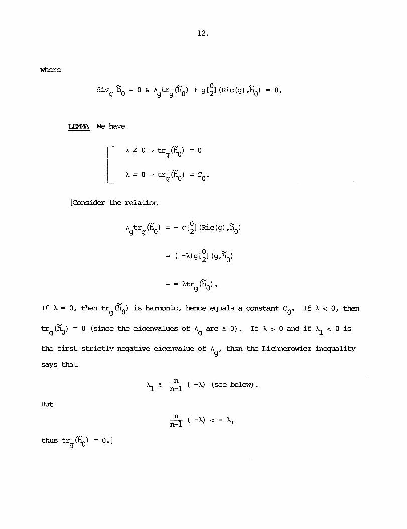
where

0 div Ii = 0 6 A tr (S ) + g[21 (Ric(g).Xo) = 0. g 0 g g o

UW4A We have

[Consider the relation

If X = 0, then tr (% ) is harmnic, hence equals a constant Co. If h c 0, then g 0

tr (E ) = 0 (since the eigenvalues of A are s 0). If X > 0 and if \ c 0 is g 0 g

the first strictly negative eigenvalue of A then the Lichnerowicz inequality g '

says that

n ? L 5 iFi ( -1) (see below) .

But

thus tr (Fi ) = 0.1 g 0

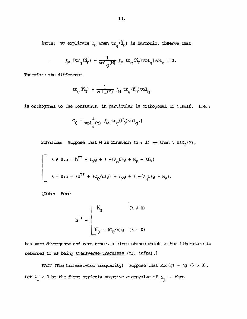
[Note: explicate Co when tr (fi ) is harmnic, observe that g 0

Therefore the difference

is ortLhogona1 to the constants, in particular is orthogonal to i t se l f . I .e. :

Scholium: Suppose that M is Einstein (n 7 1) -- then V heS2 (M) ,

[Note: H e r e

has zero divwgence and zero trace, a circumstance wh ich i n the l i tera ture is

referred to as being transverse traceless (cf. infra).]

Let \ c 0 be the f i r s t s t r i c t l y negative eigenvalue of A - then g

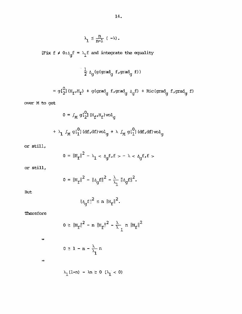
[Fix f # 0:A f = \f and integrate the e q u a l i t y 9

or still,

or still,

But

Therefore

~bservation: Let XCD' (M) , s €S2 (M) -- then

2 0 (div X ) g , s ) v o I < - - (div X ) g , s > = .fM g12]( -, n g g 9

- 2 - - - .f (div X) tr (s)vol n M g g 4

Given ga4, define

by

and define

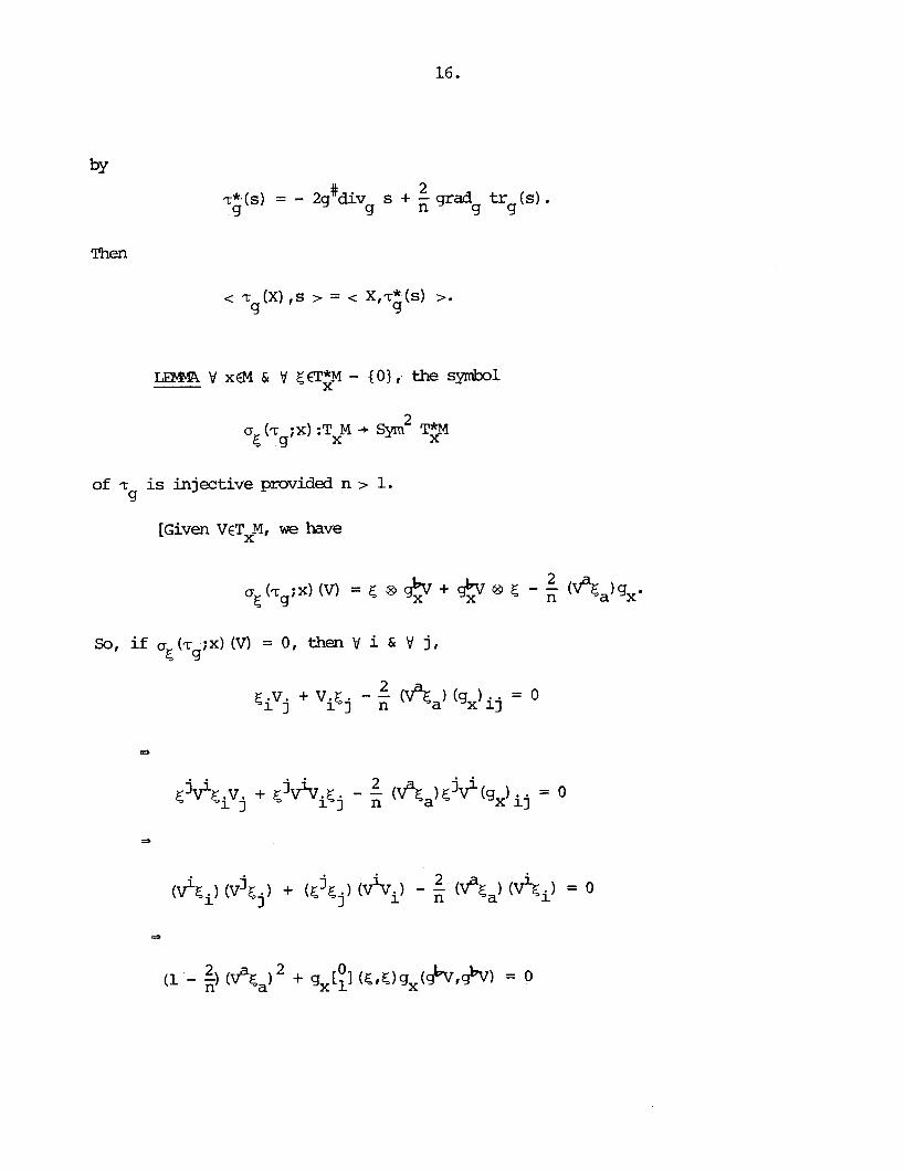
by

Then

# 2 T*(s) = - 2g div s + 9 g

- gradg trg ( s ) .

< 7; (X) ,S 7 = < x,z*(s) >. g s

LEMMA V x s l & V M - 0 , the s W ~

o (7 ; x ) :TxM + Syrn2 TEM k s

of T is injective provided n 7 1. 9

[Given VcTxM, we have

By el l ipt ic theory, it then follows that there is an orthogonal deccglrposition

S2(M) = Ran T @ K e r T*, 9 g

where both Ran z and Ker z* are closed subspaces of S2(M). 9 9

Consequently , every s €S2 (4) can he sp l i t into three parts :

Here

# 2 0 - 29 div so + ;; grad tr (s ) = 0 9 (3 g

or still,

or still,

or still,

or still,

# 1 # 0 - g d i v ~ O + ~ g d t r ( s ) = O g 9

0 1 0 - div s + - div (trg(s )g ) = 0 9 n 9

1 0 div (so - T; trg(s )g) = 0. 9

RaMlrk: A vector field X is said to be conformal i f

Every infinitesimal ismetry is c o n f o d , the converse being false in general.

[Note: According to Y a m ' s

1, [Ric (X,X) - (div

So, i f X is conformal, then

formula,

2 1 0 1 x) + 2 d 2 1 (&g,$p) - gI1I (vX,VX) lwl 9 = 0.

a relation which places an a priori restriction on the existence of X. E.g.:

There are rn nonzero conformal vector fields i f the Ricci curvature is negative

definite. 1

Put

Then

[NO*: We have used the fact that

0 tr (s) = tr (s 1.

9 9

Proof:

Notation: S2 (a) TT stands for the subspace of S2 (M) consisting of tbse

s such that

div s = 0 & tr (s) = 0. 9 9

[Note: In other words, S2 (MI TT is the kernel of the map

that sends s to (div sf* ( ~ 1 ) . g g

The preceding considerations then imply that

m k : ~t can be shown t h a t S2 (M) TT is infinite dimensional provided

n > 2.

H e r e is sarne termbmlogy tha t can serve as a recapitulation.

U l a t u r e :

(1) The spli t t ing

is called the camnical decomposition of s€S2 (M) . (2) The spli t t ing

h = + ( - ( A f ) g + Hf - fRic(g)) g

is called the BDBE deccgnposition of h€S2 (M) .

(3) The spli t t ing

TT 2 1 s = s + Lxg +, ( -div X ) g + K t r (s)g g 4

is called the York deampsi t ion of s €S2 (M) .

Section 31: Metrics on Metrics Let M be a connected cW fianifold of

dimension n. Assume: M is a m p c t and orientable and n > 1.

Rappel: M (the set of r i d a n structures on M) is open in S2 (M) , -0

hence is a F'rkhet manifold d e l e 3 on S2 (M) . Put

the pairing

< , > :TM x T*M + R g o g-0 -

being

g

0 = iM g121 ( u . v ) ~ l g .

2 2 [Note: T*g0 is the "L cotangent bundle" of Ifo (the fiber T*M = s ( M )

g-0

is a proper subspace of the toplogical dual of T M = S2(M)).] 9-0

Given PER, - define

and set

G ( u , v ) = & [ u , v ~ ~ 0 1 P 19 Pts s'

Then

is a srm0t.h symnetric bilinear form.

[Note : Obviously,

I [u,vI = [u,vI + (P- K) tr (u) tr (v) . P IS 9 s 9

Therefore

I Example: Take = - - 1 -- then G1 n ( 2 G ) is called the I k W i t t metric, - - 1 , s s n

LElWA V PfO, G is nondegenerate. P I S

[Fix u€S2(M) and suppose that G (u,v) = 0 V v€S2(14) -- then in particular B I S

We have

Therefore

Rappel: Derote by iff+^ the normal subgroup of Dif f El consisting of

the orientation preserving diffecarorphisms -- then there are tm possibilities.

[Dif f M:D~£ £+MI = 1, in which case M is irreversible.

+ 0 [Dif f ~ : D i f f $11 = 2, in which case M is reversible.

[Note: There is then an orientation reversing diffecmrphism of M and

a short exact sequence

where sM(cp) = +1 i f cp is orientation preserving and cEI(q) = -1 i f cp is orientation

reversing. ]

Remark: When equipped w i t h the cm toplogy, Diff M is a topological group.

The normal subgroup iff'^ is bth open and closed and contains DiffoM, the

identity component of Diff M.

The group iff'^ operates to the right on Go via pullback: \I cp€Diff+~,

g-cp = q*g (gCFI0).

E ' View G a s a sanirieMNlian structure on z0 ( p # 0) -- then B

[Note: In other m d s , iff+^ can be identified w i t h a subgroup of the

isometry group of (M ,G ) . I -0 B

In wha t follows, it w i l l always be assumed that p f 0.

b 2 G :S2(y) -+ Sd(EI) H e r e B ts

But

Therefore

b [Note: By construction, G is injective. ?@re is true: G~ is P fs P f s

bi j ective with inverse

given by

Observation: There is a comnutative diagram

where

Definition: A vector f ie ld X on TMo is said to be second order i f

[Note: Of course, IT T 0 X = ibo - is autamatic. 1

Let

be a vector f ie ld on - -- then X has two cmponents: X = (XI. X2) , where

I X,:go x S2(M) +S2(14). -

This said, it is then clear that X is second order i f f

X(g,s) = (s,X2(g,s)) (xl(g,s) = s)

~~snark : I£ x is second order and i f y (t) = Cg (t) , s (t) EMo X S2 (M) is an

integral curve for X, then

or, in brief,

[Note: The geodesics of X are, by definition, the projection to Blo of

its integral curves.]

Definition: A spray is a seaond order vector field X on To which satisfies

the follwing condition: V XER, -

[Note: In other words, X2 is honmgeneous of degree 2 in the variable s f

THM)REM Fix B + 0 -- then there exists a unique spray X on To 1Ose P

second component r has the property that P

[Note: The significance of this result w i l l beccane apparent i n the next

section. 1

The uniqueness of X is obvious. As for its existence, let B

where

or still,

Then

[Note: Put

Then B is bilinear and P

1 Example: Take p = - - 1 - then T1

n (G r) is called the DeWitt spray, - - n 1

thus

Consider now the RHS.

ij ij k = 2 s s hk - h s s i k j ik j'

And

Therefore

1- n + fM tr 9 (sI2trg(h)volg,

which is precisely the expression derived above for

G (rg(g,s),h). B 19

1 + (8 - K) fM tr (s) [s,hl wlg.1

g g

The governing equation for the geodesics of X is 8

Ej = r8 (g,&

or, written out,

RePMlrk: This equation is an ODE and the evolution of a solution g ( t )

depends only on

- g (0)

- &o) . To be precise: Given (g ,s 1, there exists a unique integral curve 0 0

y:]- c . E [ -+ zo x S 2 ( ~ ) for X such that y(O) = (gO,sO), i.e., P

[Note: The geodesics can be found explicitly but the formulas are not

particularly enlightening (they do show, however, that the geodesics exist for

a short time only in that they eventually run out of E0 into S2(M) ) .

Section 32: The Symphctic Structure Let Y be a connected cm r'oanifold

of dimension n. Assume: M is campact and orientable and n > 1.

Rappel: There is an arrow of evaluation

and a nondegenerate bilinear functional

viz .

Consider T*r+, - = Eo x S: (M) -- then

The Canonical 1-Form O This is the map

defined by the prescription

The Canonical 2-Form P T h i s is the m p

defined by the prescription

LEWA We have

52 = - do. [In fact,

Therefore Q is exact and the pair (T*ZO ,Q) is a symp1ectic manifold.

Fix p # 0 and define

O p q , ' T*P20

Then 4 is an i m r p h i s n of vector bundles, hence a

is mndegenerate. On the other hand,

which implies that Q is exact. P

Conclusion: The pair (TM ,Q ) is a symplectic manifold. -0 P

[Given Pi # 0 (i = 2 , the bijection

is a car#,nical transformation:

For the LHS equals

SUBLEMMA The tangent map

is given by

[Note: Since

it follows that

where

Explicated :

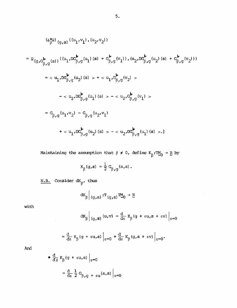
Maintaining the assumption that p # 0 , define K :TM0 + B - 1 K ( g , ~ ) = - G ( s , s ) .

B 2 PI57

N.B. Consider dK thus B '

with

THEOREM For all vector fields X on TMO, -

Interpretation: Per 8 X is a hmniltonian vector field on Two with P' P

energy K P ' FACT (Conservation of Energy) Let y(tl be an integral curve for X --

B then the function t -+ K (y (t) ) is constant in t .

B wmply note that

1 Construction Let XfV (PO -- then X induces a vector field 2 : ~ ~ -+ S2 (M) - on so via the prescription

Put at = 42, where +t. is the flow of X -- then there is a ccmutative diagram

Here

and

SUBLEMMA W e have

KB = KP =t-

Application: A t any p i n t (g, s) €9, -

Rappel: A f i r s t integral for a vector f ie ld on To is a function

£:Dlo - + R - which is constant on integral

So, e.g., K is a f i r s t integral P

curves.

XP

1 LEMMA V XED (M) , the function

(9,s) + G P r g ( ~ J X 9 )

is a f i r s t integral for X P '

[Let y ( t ) = (g( t ) ,s(t) ) be an integral curve for X - then 6 = s and P

or, restoring the dependence on t,

d - G 1 d d t B,g(t>

( ~ ( t ) ,h) = - - G 2 de p,g(t) + eh E=O

Now replace h by k g (t) -- then

But

Theref ore

W r i t e

1 = - 2 IEl div (S + ( -. ) (slg) (X)volg. 4 9

Let

1 n ( s ) = s + ( $ - - ) t r ( s ) g . P ,g n g

Then it fol lms that the function

(g , s) -+ JM div (n (s) 1 (XI volg 9 PIS

is a f i r s t integral for X P '

Conservation Principle Suppse that y (t) = (g (t) , s (t) ) is an integral

curve for X Abbreviating n P ' P,s(t) (S (t) ) to n P (t) , v X&M) ,

JM div n (t) (XI volg (tl g ( t ) P

is a constant function of t, which implies that

div n (t) e lg(t)11/2~A(M) s(t) P

is a constant function of t. Consequently, i f

divg(0)ng (0) = 0,

div n (t) = 0. g ( t ) p

Section 33: mtion in a Potential Let M be a connected coo manifold of

dimension n. Assume: M is canpact and orientable and n > 1.

Given NEC- (Y> , put

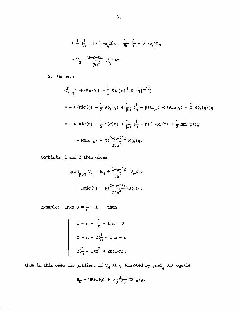
2. We have

Combining 1 and 2 then gives

Example: Take

I -

thus i n th i s case the

1 - n - (: - l ) n = o

2 - n - 2(;- l ) n = n

gradient of VN a t g (denoted by grad V ) equals g N

[Note: When N = 1, the hessian drops out and there ramins

S(g1g.I - a c ( 9 ) + T(~~;IT

Define a vector field

v 1. = (sJg(9 .s ) - gradgrg N

Then Y is second order and the equation determining its geodesics reads BIN

l a n d N = l - - t h e n Example: Take 8 = - - n

THEDRIDI For a l l vector fields Y on TMot

Qg (Yp INIY) = dE B , N ( ~ )

where

E = K +VN. P I N P

[Suppose that Y (g , s ) = (u,v) -- then

Bearing in mirad that the pair (TM B ) is a symplectic manifold, it follows -0' p

that Y is a hamiltonian vector field on TJo with energy E P I N $ IN*

[Note: A s before, energy is conserved, i.e., on an integral curve

y ( t ) for Y $ INf

the function t -t E ( y (t) ) is constant in t .I BIN

Take N = 1 a d write V in place of V1, hence

and

1 LSEMA W XCD (M) , the function

(grs) - G (s,Lxg) P r s

is a f i r s t integral for Y (E Y ) . B B f 1

[The only new point is that

1 is a f i r s t integral for Y But XED (M) is arbitrary. So, along an integral 8 '

curve y( t ) for Y B '

is necessarily a constant.

Notation: Let

n (s) = s - trg(s)g. '3

Then

1. for the choice p = ;;; -

Ll3W.i W e have

- A tr (s) - 6 div s = - 6 div rr (s). g g g 9 g ' 3 9

[In fact,

- A tr (s) = - div grad tr (s) 9 g 9 4 4

# = - div g (dtr (s)) g '3

Therefore

- A tr (s) - 6 div s g g g g

= 6 div (trg(s)g) - 6 div s g '3 9 g

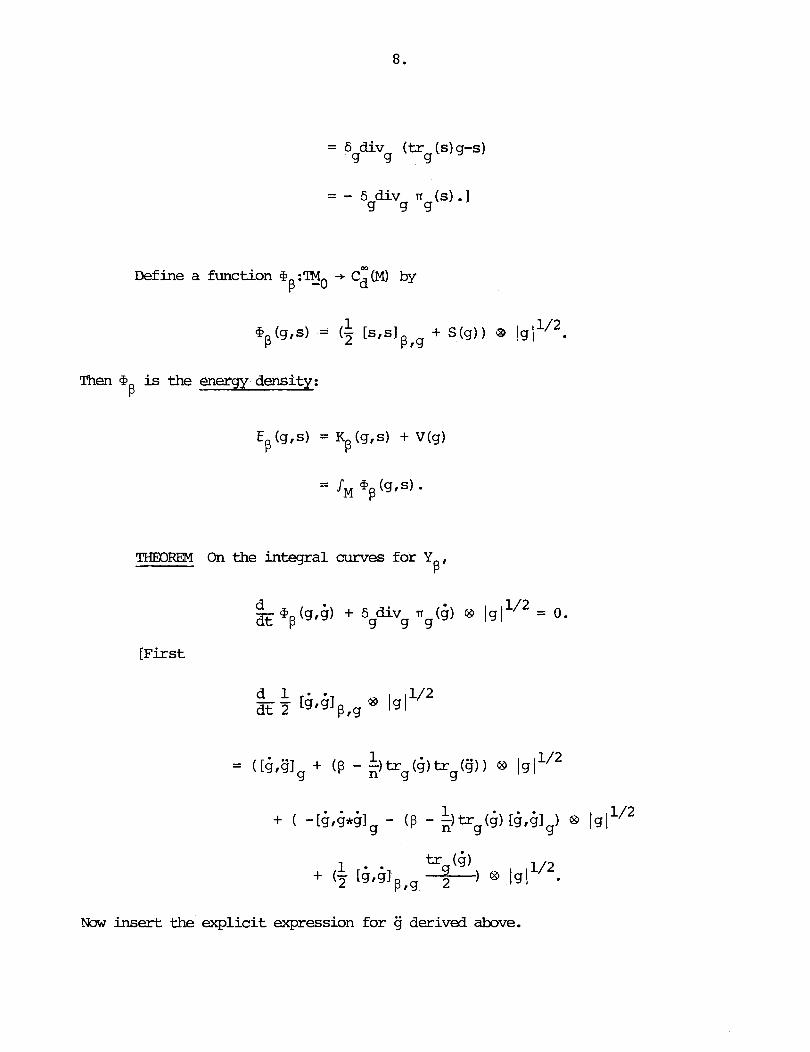
= 6 div (tr (s)g-s) g g g

= - 6 div n (s) . ] g 5753

Define a function .P :TMo + c ~ ( M ) by B

Then cP is the energy density: B

THEOREM On the integral curves for Y B '

[First

Now insert the explicit expression for g derived above.

1 ( p - -)tr (4) t r (g) is the sum of f i ve t e r m s : n 9 g

1 2-n-2811 1 0 p - 1 zpn

. . . There are t w o imnediate cancellations, viz. term 1 cancels with - [g,g*g]

1 and term 6 cancels w i t h - ( p - ---) trg (6) [4,41 Consider next term 3 and term 8

g '

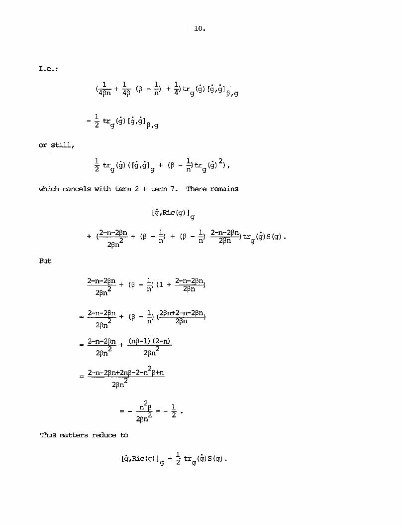
or still,

which cancels with term 2 + t e r m 7. There remains

But

Thus matters reduce to

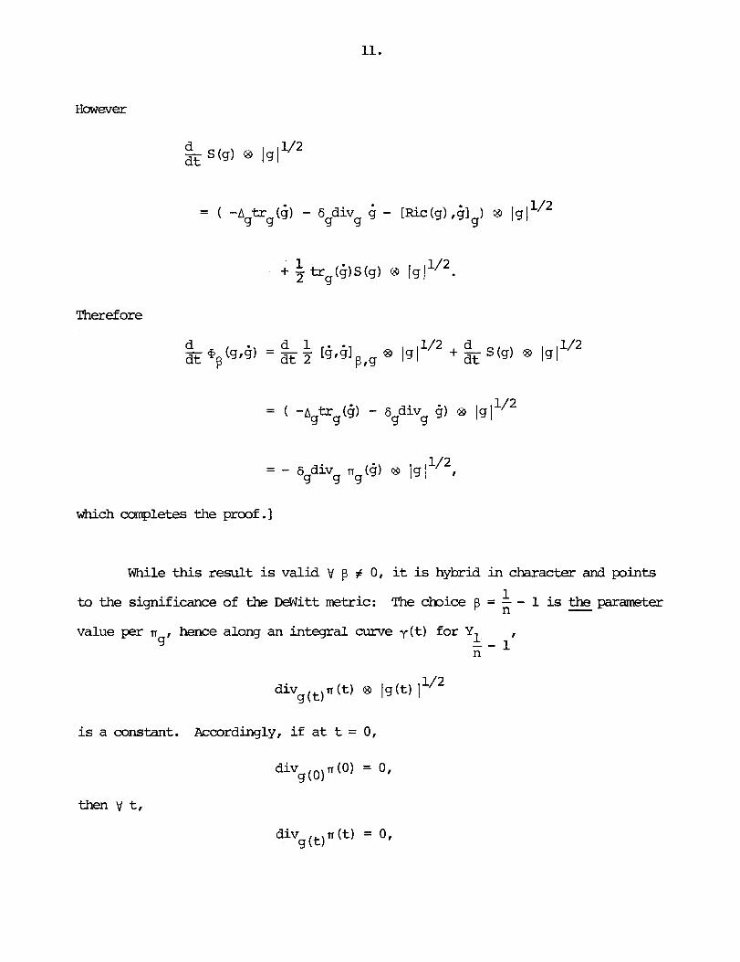
However

Theref ore

which mnpletes the proof. 1

While this resu l t is valid V p # 0, it is hybrid in character and points

to the significance of the Mitt metric: The choice p = - - 1 is the parameter n - value per n hence along an integral curve y ( t ) for Y1 I ' - -

n 1

is a constant. Accordingly, i f a t t = 0,

thus

and so el is pointwise constant in time. - - n 1

RBwk: Let C be a nonzero constant. Replace V by CV (a.k.a. VC) and

Then, on the integral curves of Y BtC '

Let

Then

LDlM& We have

[Since

it follows that

Theref ore

-1 " ((9,") = (g,8 $ t S ( A ) ) .

2 Thus the coefficient of tr (s) i s

9

or still,

1 Example: Take p = - - 1 -- then n

# i f n = s w 1 1 'I2, which inplies that

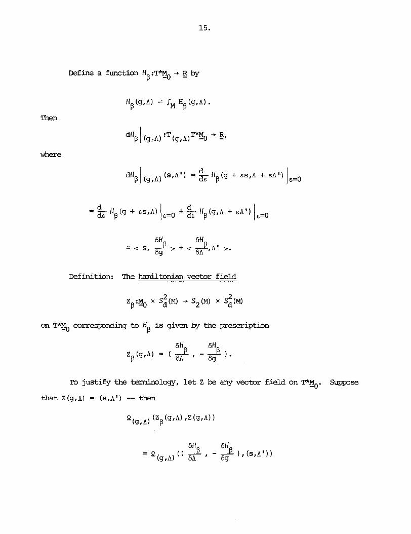
Then

where

Define a function ff :T*M -+ R by p -0 -

Definition: The hamiltonian vector f ie ld

on T*g0 mrrespording to H is given by the prescription P

To justify the tamhology, let Z be any vector f ie ld on T*zo. Suppose

that Z (grA) = (s,dl) -- then

Observation: The diagram

carmutes.

Therefore

(4 *y = z B B B '

bbreover, i f y ( t ) is an integral curve for Y and c ( t ) is an integral cwve B

for Z and i f 4 y(0) = c ( O ) , then + y(t) = c ( t ) , hence the projections of y ( t ) S B B

and c ( t) onto Eo coincide.

Remrk: Hamilton's equations are, by definition, the system of differential

equations defined by Z B '

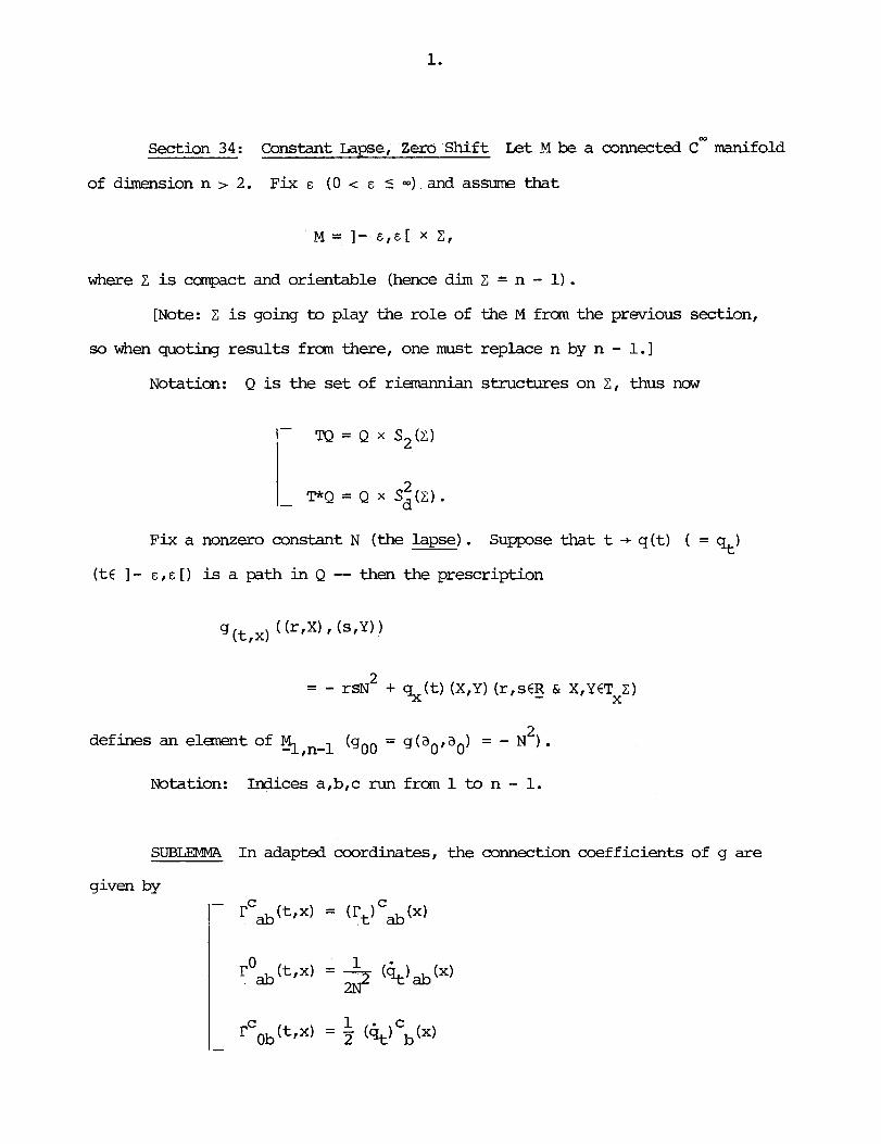
Section 34 : Constant Lapse, Zero Shift Let M be a connected C- manifold

of dimension n > 2. Fix E (0 < E 5 00) and assume that

where Z is ccgnpact and orientable (hence dim 2, * n - 1) . [Note: Z is going to play the role of the M £ram the previous section,

so when quoting results £ram there, one must replace n by n - 1 . 1

Notation: Q is the se t of riesnvlnian structures on Z, thus now

Fix a nonzero constant N (the lapse). Suppose that t -+ q ( t ) ( = qt)

( t E I - E , E [ I is a path in Q -- then the prescription

2 defines an elanent of %,n-l (goo = g(aot aO) = - N ) .

Notation: Indices a,b,c run £ram 1 to n - 1.

SUBLEPPIA In adapted coordinates, the connection coefficients of g are

given by

and

T H M ) m Ric(g) = 0 i f f satisfies the differential equation

and the constraints

We shall start w i t h the assumption that Ric(g) = 0.

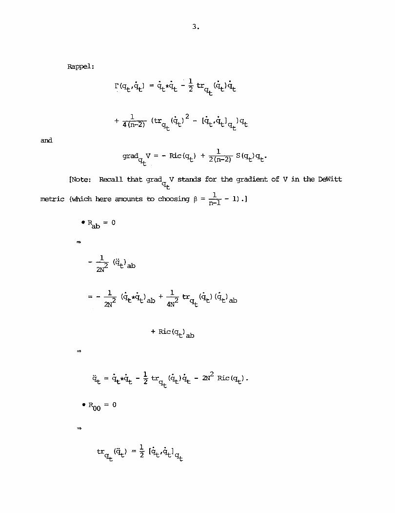
Rappel :

and

[Note: Recall that grad V stands for the gradient of V in the Mitt %

L

metric (which here armunts to choosing = = - I).]

L L

Therefore

But then

as claimed.

[Note: Since

CI

it follows

L 2N grad V = - g,

L

that the curve t -t q ( t )

( - 2 ~ ' grad 9c V )

grad V qt -2N2'

(tE I- E , E [ ) is a geodesic per

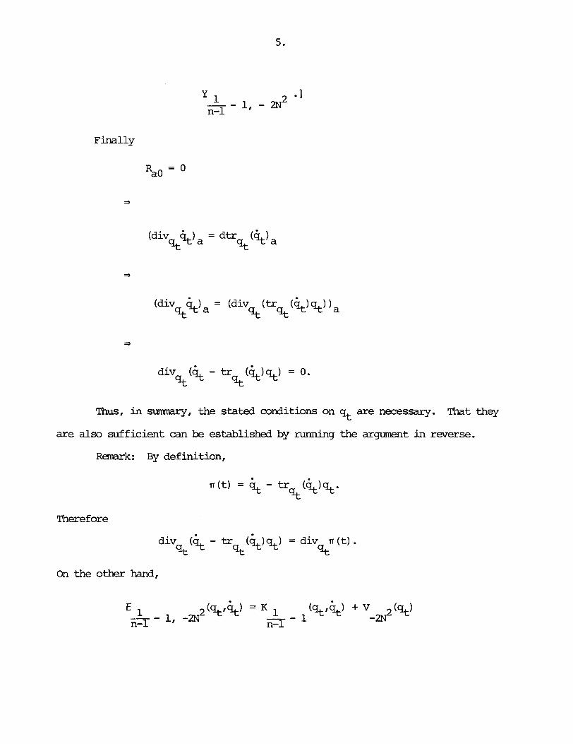
Finally

(div a = dtr a st st

(div $)a = (div st

(tr ($st''a st s,

Thus, in surmmry, the stated conditions on qt are necessary. That they

are also sufficient can be established by running the argument in reverse.

Remark: By definition,

Therefore

div ($ - tr (<)%) = div n (t) . s, s, st

On the other hand,

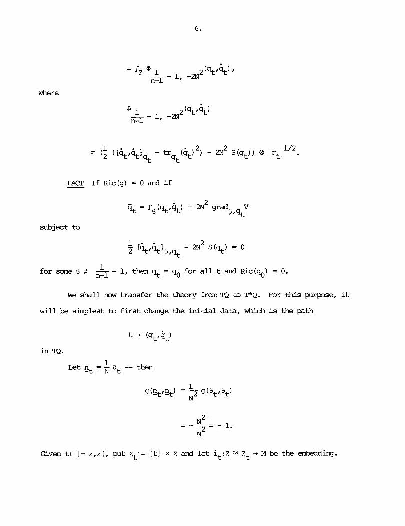
where

FACT If Ric (g) = 0 and i f

;t = rg (qt, + 2NL grad B I q t V

subject to

W e shall now

w i l l be simplest to

1, then qt = qo for a l l t and Ric(qo) = 0.

transfer the theory from TQ to T*Q. For th i s purpose, it

first change the i n i t i a l data, which is the path

in TQ.

Given t€ 1- E ,E[ , put Zt = {t) x Z and let it:z Zt -+ M be the M i - .

Working w i t h the metric connection of g, let ut€S2 (2) be the extrinsic curvature,

thus

xt (VIWl = % ( -i;V&,w) g (q,ql

[In fact,

So, instead of the path

we can just as w e l l work w i t h the path

Definition: The nnnentum

defined by the prescription

2 of the theory is the path t + pt in %(Z)

where

[Simply observe that

Theref ore

$=at

Consider the relations figuring in the theorem, beginning with the constraints.

In terms of ut, this reads

div (2Nxt - 2NKtgt) = 0 st

or still,

div (xt - Ktqt) = 0. st

But div pt is, by definition, st

1/2 div (xt-Ktqt) !;9 , q t

thus our constraint becares

div pt = 0. s,

In t e r m s of ut, this reads

or still,

or still,

or still,

or still,

or still,

whexe we have set

It remains to reformulate the differential equation

2KIL grad V %

in terms of pt.

We have

where

Formulas

- # x# = ((i # - 4N(xt*xt) . d t t

TO isolate it, one need only divide % by 2 N .

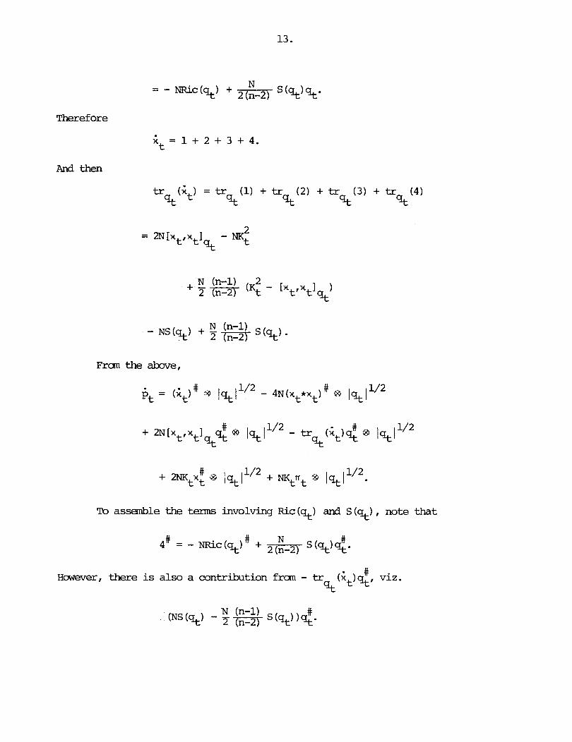
Theref ore

Andthen

Fram the above,

'~b assanble the tm involving Ric (st) and S (s,) , note. that

# Huwever, there is also a contribution from - tre (Gt) qt, viz.

But

- - N 2-n + 1) = 2. N(2 (n-2)

Thus we are l e f t with

Next

which leaves

# -NKx + N t t 2(n-2)

N (n-1) 2 - - - - 2 (n-2) (Kt [xtfxt

Now collate the data and colleat t e ~ ~ n s .

# The coefficient of Ktxt is

- N + 2 N + N = 2 N e

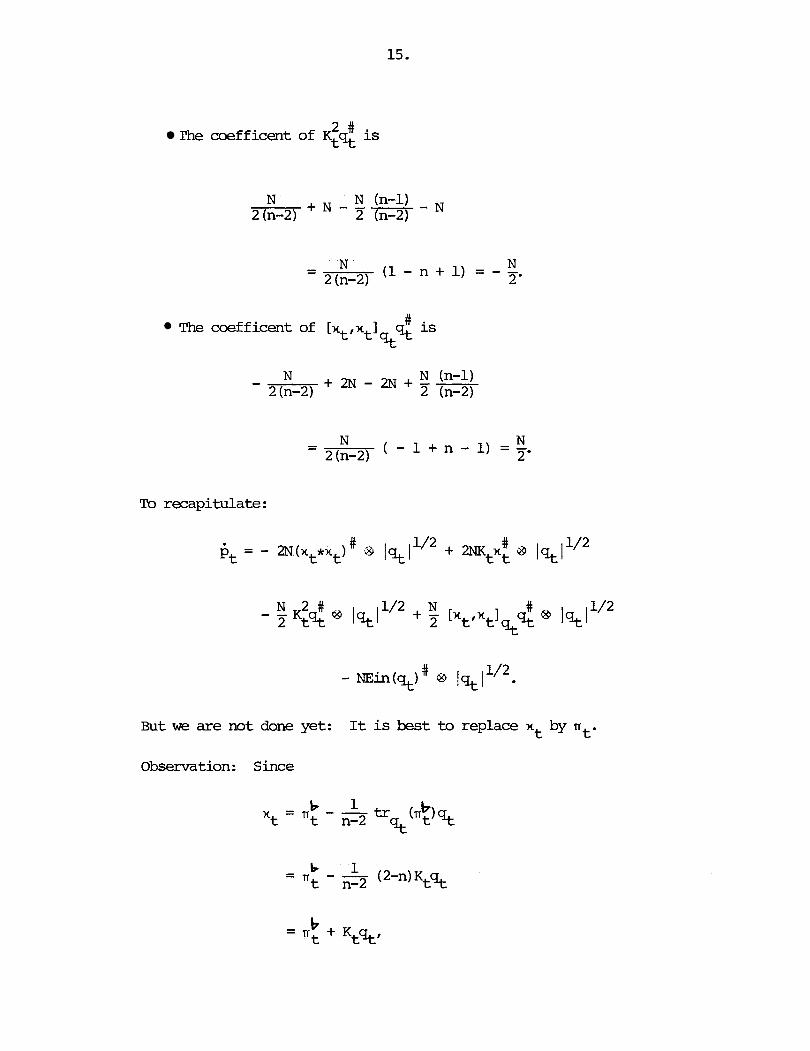
2 # The coeff icent of Kt% is

# The coefficent of [ntfxtlstst is

To recapitulate:

But we are not done yet: It is best to replace xt by fit.

Observation : Since

where, by definition,

Theref ore

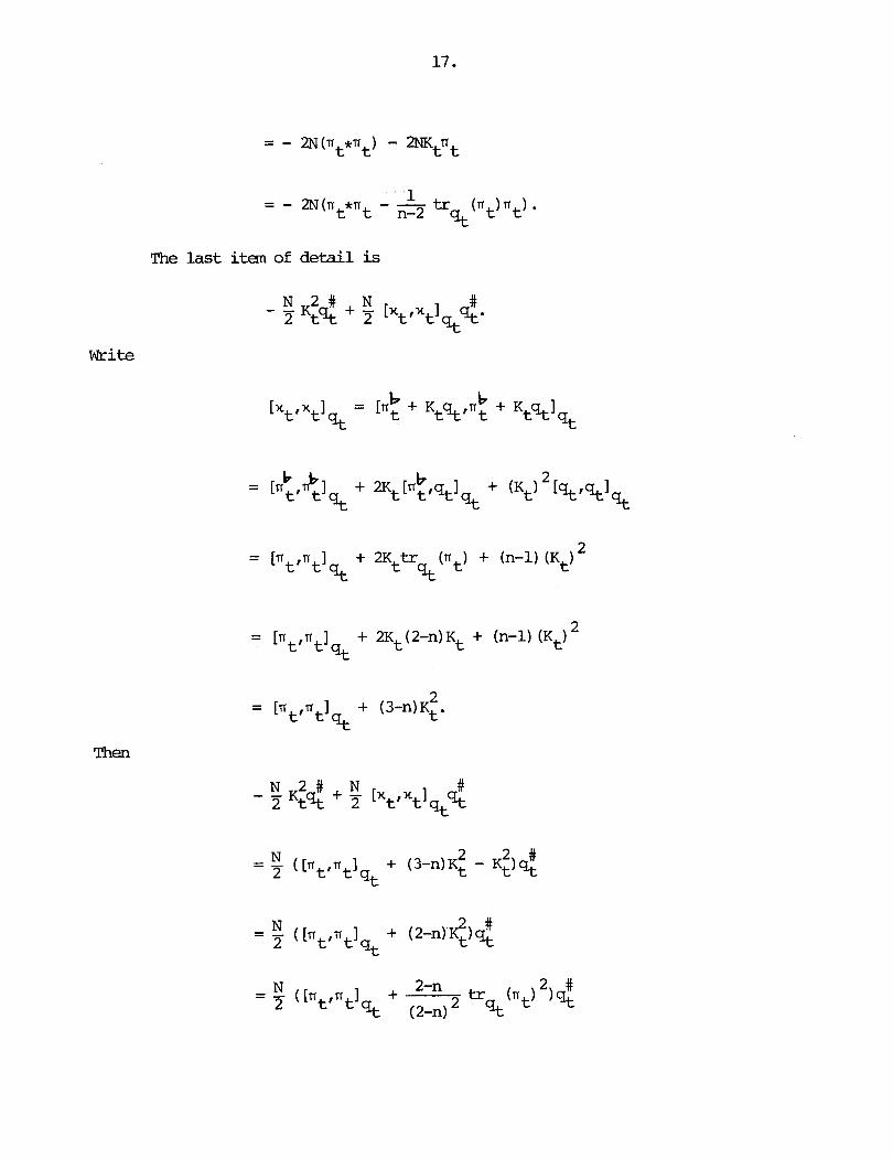
The last iten of detail is

N K 2 # + N W - 2 tst T [Xt'xtlst%*

Write

Then

N = - ( [n ,rr 1 - - 2 t t qt n-2 st

Sumnary: We have

- 2N(ut* ' r t - - bt - - n-2 tr (n ) n 8 ~ q t j " ~ s t t t

N 1 / 2

# 1/2 - N E i n ( q t ) @lqtl .

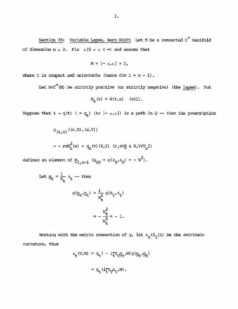
Section 35: Variable Lapse, Zero Shift L e t M be a connected C- manifold

of dimension n 7 2. Fix E (0 < E 5 "1 and assume that

where 2 is compact and orientable (hence dim 2 r n - 1).

Let N€cm (M) be s t r i c t l y positive (or s t r i c t l y negative) (the lapse) , Put

Suppose that t + q ( t ) ( = qt) ( t 6 I - E ~ F I ) is a path in Q -- then the prescription

2 defines an element of Ml,n-l - (goo = g(aoIao) = - N ) .

1 L e t nt = - at -- then - Nt

Working with the metric connection of g, let xt€S2(z) be the extrinsic

curvature, thus

xt(VIW) = gt( - i;V&,W)g(gIgtt)

And, as in the case of constant N,

Remark: The focus below w i l l be on the canputation of ; rather than q. t

A t each t, sulsananifold theory is applicable to the pair (M,Z) (per - g = iXg = %). To help keep things straight, overbars are sanetimes used to t

distinguish objects on Z £ran the corresponding objects on Y.

LET4MA In ada~ted coordinates (and abbreviated notation), the connection L

coefficients of g are given by

and

[The ccsrrputation is carried out using

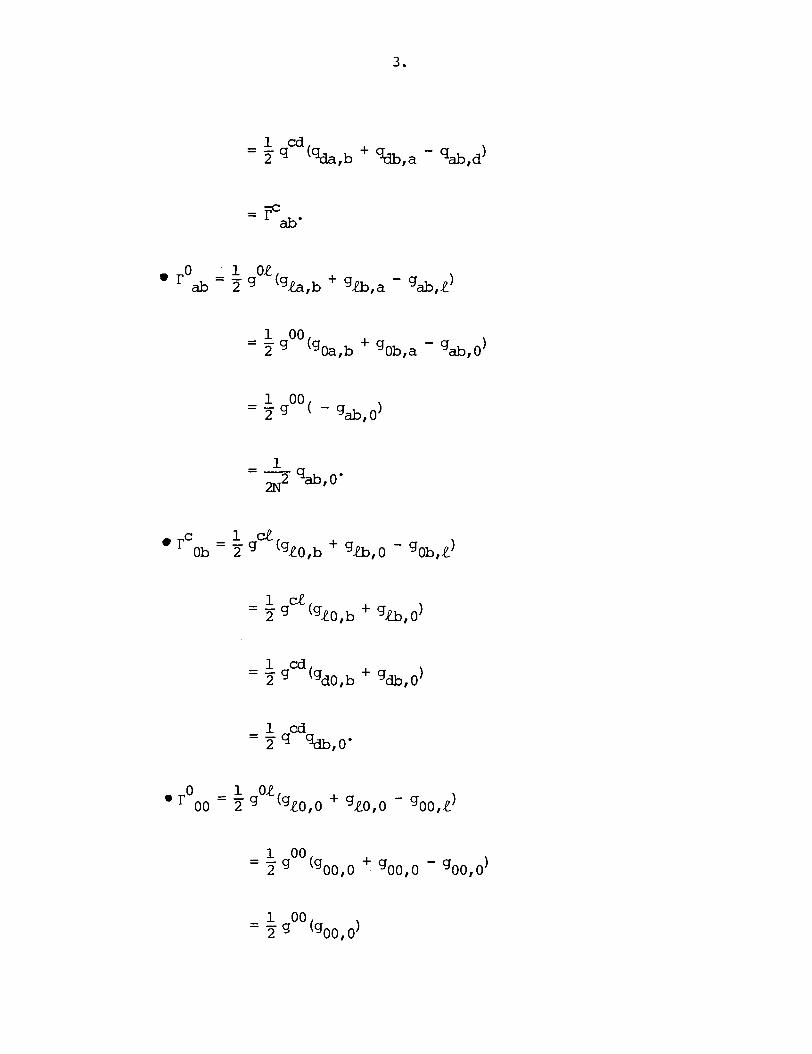
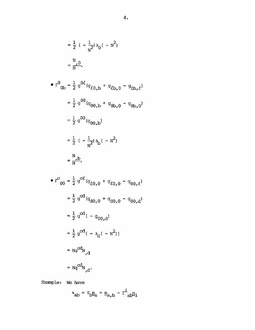
- 1 cd - 3 (gdOtO + gdO,O - gOOtd)

- 1 cd - 29 ( -

1 ad 2 = p ( - a d ( - N 1 )

= " P N d

= Nq 5 t d'

m p l e : W e have

- nab - V g a = n i - I' *ni -a,b

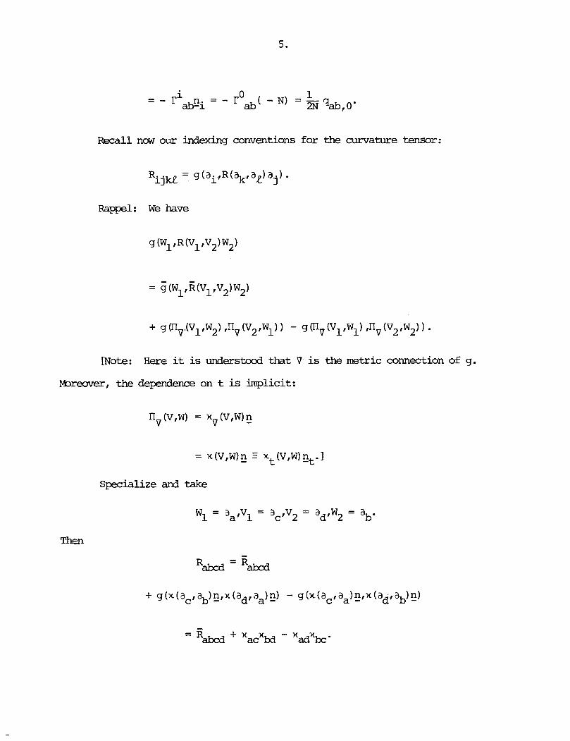
Recall now our indexing conventions for the curvature tensor:

[Note: Here it i s understood that V is the metric connection of g.

mreover, the dependence on t is implicit:

Specialize and take

Then

Rappe l : W e have

or still,

= (B n) (v1,w) - (5 x) (v~ ,w) . v2

- [Note: V is the mtric connection of g , hence is torsion free. Therefore

Details It is a question of supplying the omitted steps i n the preceding

manipulation. To begin wi th ,

On the other hand,

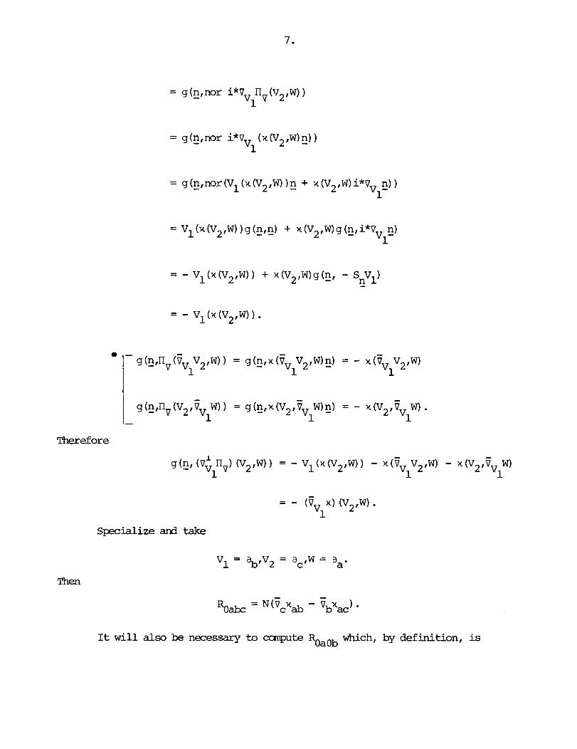
0

Therefore

Then

Specialize and take

It will also be necessary to canplte ROaOb which, by definition, is

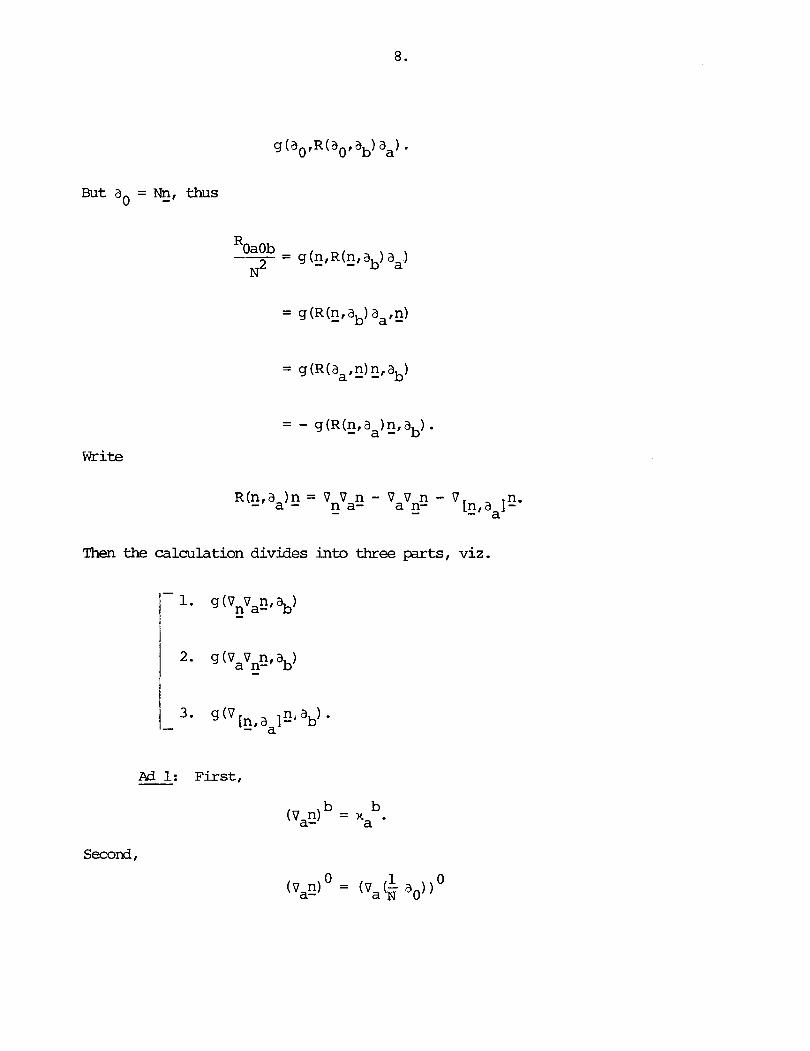
Then the calculation divides into three parts, viz.

Ad 1: Fi r s t ,

Second,

Theref ore

Ad 2: Analogously, -

Ad 3 : On the one hand,

[n,aalC - = 0,

while on the other,

Now combine terms:

THEDm Ric(g) = 0 iff nt satisfies the differential equation

; = 2N (X *X ) - N K x - NtRiC(%) + % t t t t t t t t

and the constraints

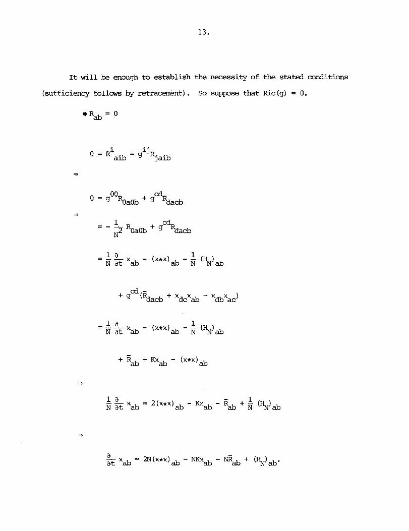
It will be enough to establish the necessity of the stated conditions

(sufficiency follaws by retracement) . So suppose that Ric(g) = 0.

00 O = g R OaOb + .".dad3

; = ZN (x *x ) - N K x - N t F l i c ( q t ) + % . t t t t t t t t

i - i j O = R Oia - R j ~ i a

But

- b

(div x) a = Tbn a 9

Therefore

div (x - Kq) = 0. 9

div (x, - KA) = 0. st

The necessity of the stated conditions is thereby established.

Observation:

2 Ix,, xtI - Kt = S (qt)

st

K = 2N (X *X ) - N K x - NtRiC(s) + % t t t t t t t t

=2N ( M * u ) - N K x + Nt 2 t t t t t t 2 (n-2) (Kt - [xt~xtlqt)st

2 Definition: The manentun of the theory is the path t + pt in Sd(z)

defined by the prescription

where

The discussion in the previous section can now be repeated virtually

verbatim.

Constraint Equations These are the relations

div pt = 0. st

Evolution Fquations These are the relations

and

[Note: The explanation for the appearance of the laplacian A Nt is st

the fact that tr (Gt) figures in the formula for &.I st

Section 36: Incorporation of the Shift Let M be a connected cm manifold

of dimension n > 2. F ix E ( O < E 5 m, and assume that

where Z is campact and orientable (hence dim 2 = n - 1) -+

Definition: A shi f t is a time dependent vector vield N on ,Z (thus

-+ + 3

N:]- E , E [ -+ TC has the property that Nt(x) = N(t,x)ETxZ V xEZ).

3

Fix a lapse N 3nd a sh i f t N. Sup~ose that t -+ q ( t ) ( = %) ( t€] - E , E [ )

is a path i n Q. Then the prescription

defines an element of %In-l. -+

[Note: In adapted coordinates ( w i t h N = ~ ~ a , ) ,

and

Rgoark: We can w r i t e

+ + +b g = - (N2 - q(~,N))dt 63dt + N W d t + dt @zb+ q,

modulo, of course, the obvious agreements.

l a + Let nt = - (x - Nt) -- then - Nt

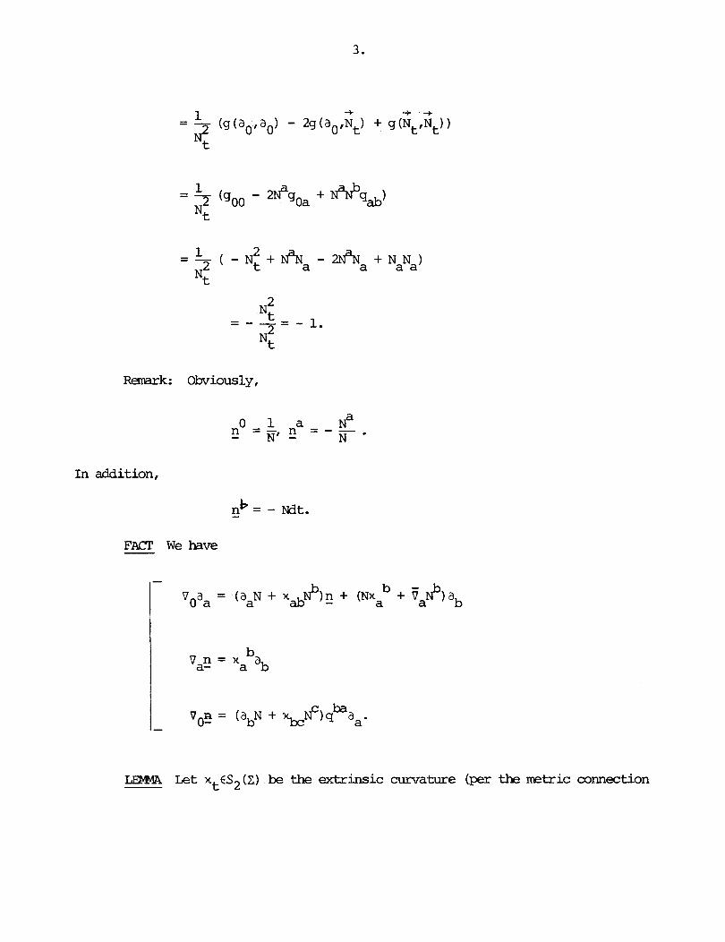
1 = -T (goo - 2Nagoa + Mq*)

Nt

m k : Obviously,

In addition,

nb - = - ~ d t .

FACT We have

LEWA L e t nt€S2 (2) be the extrinsic curvature (per the m t r i c connection

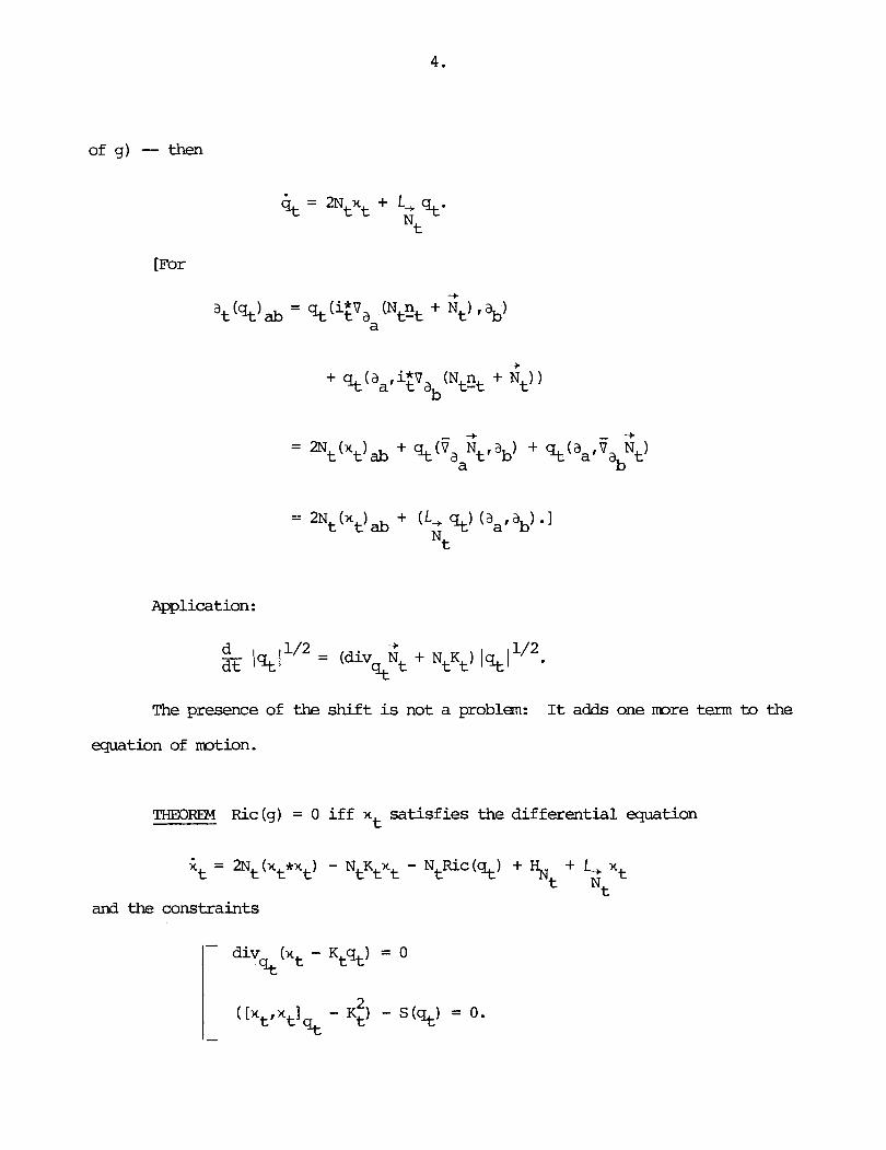
of g) -- then

[For

= a t (X t a b +qt(~aaGtlab) +q,pa1o ab

Application :

The presence of the shift is not a problem: It adds one more term to the

equation of rmtion.

THEOREM Ric(g) = 0 iff xt satisfies the differential equation

i = 2N (x *x ) - NtKtxt - NtRic(qt) + % + L, xt t t t t Nt

and the constraints

div (xt - Kt%) = 0

A p a r t f r m a few additional wrinkles, the argument runs along the by now

familiar lines.

0 ' aOb

- 1 C - - g - Nua nd - %TaNC - vb(TaN + naCNc) I .

[In fact,

0 ' aOb = dt(vovbaa - VbV~aa)

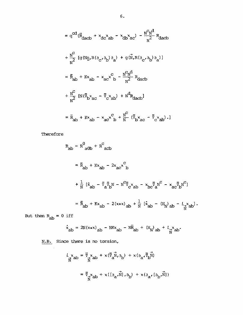
Therefore

- 0 C

Rab - aOb + acb

- 1 . = Rab + Kxab - 2 (x*x) ab + N [X * - (HNIab - I!. 1 -

G a b But then Rab = 0 i f f

Gab = 2N(x*x)* - NKxab -

N.B. Since there is no torsion,

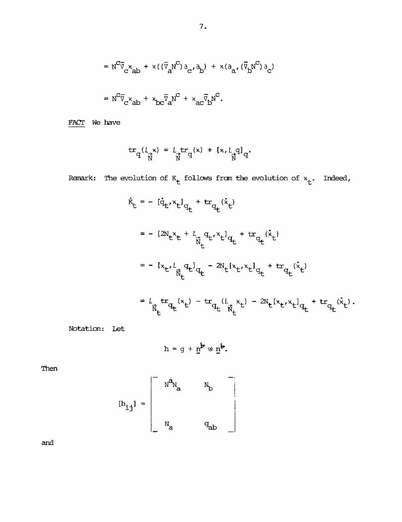
FACT We have

RBnark: The evolution of Kt follows £ran the evolution of x Indeed, t'

Notation: Let

Then

and

To discuss the f i r s t constraint, write

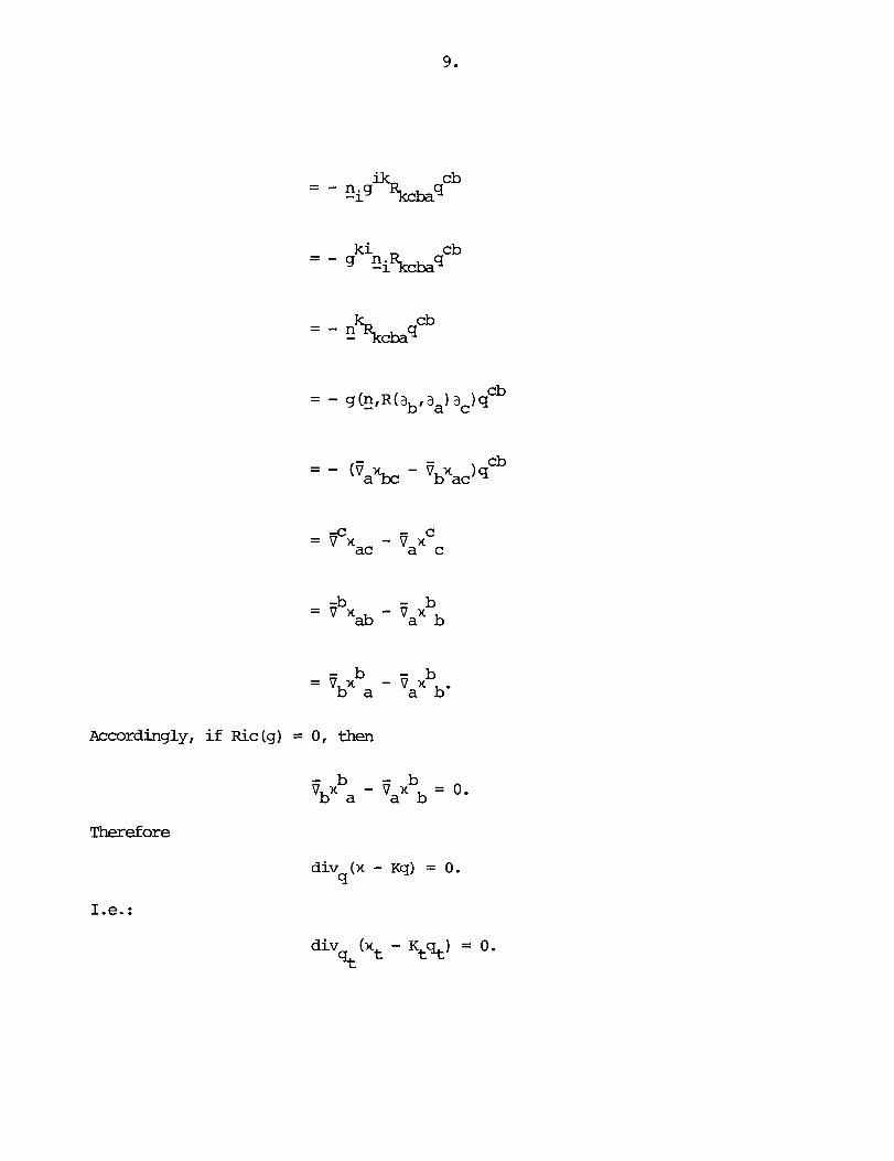
- - b - b - Vbx a - van

Accordingly, if Ric (g) = 0, then

- b - b Vbx a - Van = 0.

Therefore

1.e. :

div (x - Kq) = 0. 9

div (xt - Kt%) = 0. st

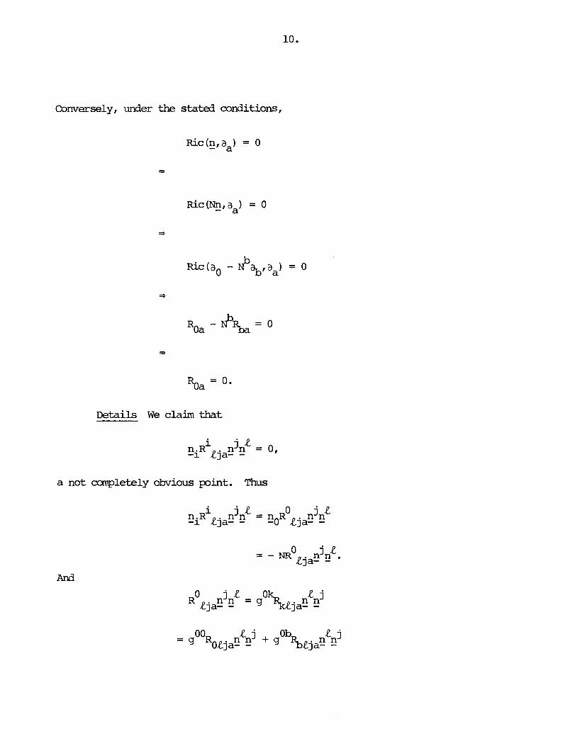
Conversely, under the stated conditions,

And

- 0 0 00 O0 n n + g 0 d -

R ~ ~ ~ a - - 2

00 c 0 00 c d n n + g Rod: n

+ g R ~ c ~ a - -

Ob 0 0 Ob 0 d + g %OoaG rt + g RbOdar! I1

Ob c 0 Ob c d + g s o a n + g %&? E

R ~ ~ ~ a = 0 & Ram = 0.

c 0 O0 n n R ~ c ~ a - -

- 00 c 0 - g rt I1 ROcOa

- 1 - - - . N2

N~ = - R N4 OcOa

- Nb - - 4 % O O ~ * N

But

But

This leaves

And

But

- - Oc b 0 - g n n R - - abco

On the other hand,

Obc 0 - NbNc g n n - - - .

N*

Consequently,

And

' a h + R~ + R~~ = 0.

But

- - - N'NbNd N4

On the other hand,

Ob c d - N ~ N C N ~ s 2 : - N4

Consequently,

Ob c

Turning now to the second constraint, write

i j ke S(g) = R f i j p g

- k & - Rikj.t (hi' - ninj) - - (h" - n - g 1

- - Rikjeh i j h ki? - 2R k fijn i j " (see below)

So, if Ric ( g ) = 0, then Ein (g) = 0, hence

or still,

Conversely, under the stated conditions,

1 Ric (g,g) + 3 S (g) = 0

Details The claim is that

k e i j = - %Ljh n - n -

= - RRRikjh k e i j g g .

- RikjeG i j k R " 5

- i j k k - - siRj2 Z Q E

- i j k R - - RRikjn - n - g g .

i j - 2 ~ ~ , ~ g g

i j = - zgI%tRRikjn - n -

k R i j = - 2(hM - g g )RRRikjz g

mtters thus reduce to showing that

Theref ore

i j k L RL*j" " ""= O*

LEMW We have

[As was noted above,

But

Therefore

Formulas

i j vi(n v.n - 3-

i = dx (vi

= dt(vo(IQ,) + dxa(va(%)

i acN cd = dx milT q ad])

acN cd a acN cd = dt(- N q vOad) + " (ParT q ad])

acN cii 1 acN c a = -5 q (adN + + v ~ ( ~ PN) - x a~ N N

1 -a- - - - V VaN

- - I A N . - N q

Substituting these relations into the lemoa then gives

S(g) = S(q) - 3[x,xl + K 2

q

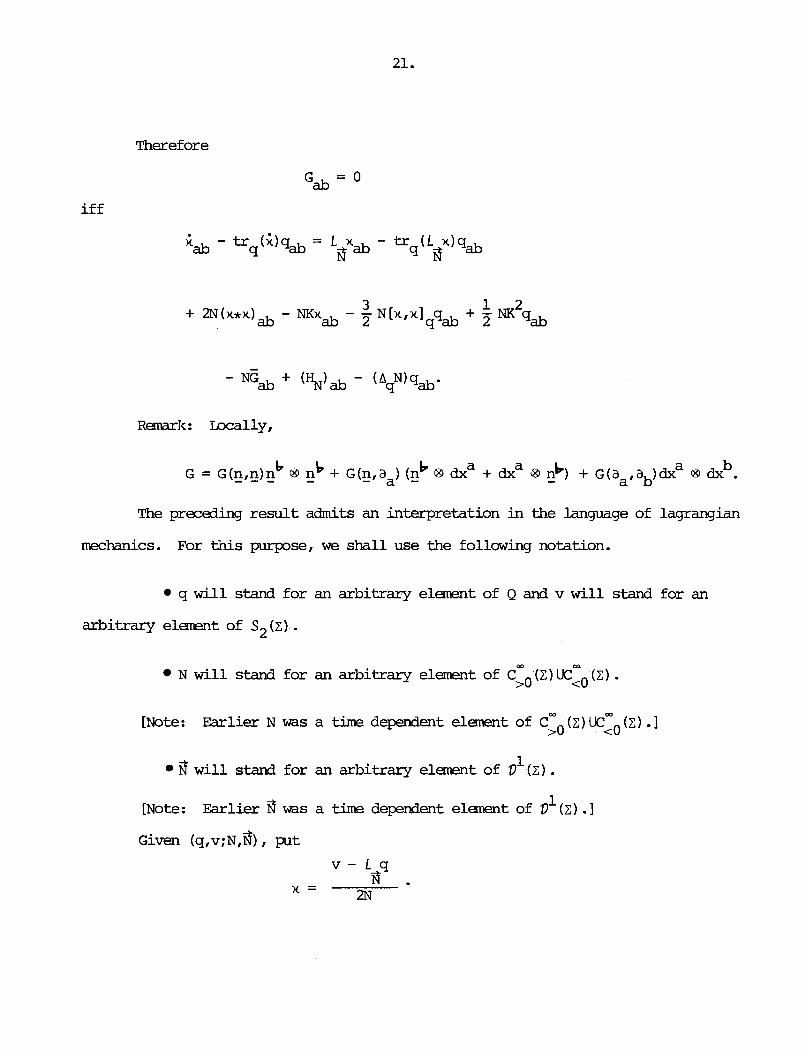
Therefore

i f f

b G = ~ ( n , n ) n ~ - - - 03 nb - + G(n,aa) (nb €3 dxa + dxa 8 nb) - + ~ ( a ~ , a ~ ) a x " 03 dx .

The preceding result admits an interpretation in the language of lagrangian

mechanics. For this purpose, we shall use the following notation.

q w i l l stand for an arbitrary element of Q and v w i l l stand for an

arbitrary element of S2 (2) .

N w i l l stand for an arbitrary element of cZO (2) wZO (2) .

[Note: Earlier N was a t h e dependent element of cZO (c) UCZO (2) .I

m 8 w i l l stand for an arbitrary elanent of D' (Z ) . 1 [Note: Earlier 8 was a t i m e depmdent element of V ( 2 ) . I

Given (cJ,v;N,~) , put

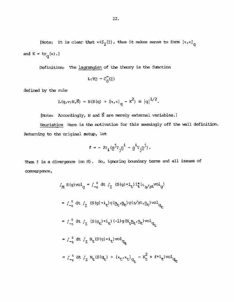
[Note: It is clear t h a t x€S2(2), thus it rrakes sense to form [x,x]

and K = tr (x) .I 9

Definition: The lagrangian of the theory is the function

L:TQ -+ c ~ ( z )

defined by the rule

L(~,v ;N,%) = N ( s ( ~ ) + [x,xlq - K ~ ) ~1 1 ~ 1 ~ ' ~ .

[Note : Accordingly, N and 8 are merely external variables. I

Heuristics H e r e is the mtivation for th is seemingly off the w a l l definition.

Returning to the original setup, l e t

Then f is a divergence (on M ) . So, ignoring boundary terms and a l l issues of

convergence,

+ = r-: at r, L(~~,&:N~,N~).

[Note: Working in adapted coordinates,

vol = ~~ll/~dtndx' A ... A cb?-l, 9

thus

dtk a/at~olg

1 = lg 1 'l2dtz~ dtn (dx A . . . a / a t A dx"-l)

= vol .I 9

Let

Ekample: Consider the simplest case: N = 1, 8 = d -- then

Notation: Write

SL - -- SL ab (q) and - 6L - - SL

(=) 6%b 6vab

[Note: On general grounds,

6L 2 6L 2 - 6sd(z) and csd(z) - 1 &I

S- We have

SUEU3.IMA We have

Consider now the original situation, viz. the t r iple (q,, ~ ~ ~ 3 ~ )

( t E ] - . s f & [ ) -- then insertion of this data into the f o m l a s for the functional

derivatives leads to t m functions of t:

6 L 6L (t) . (t) & - 6qab % b

THEOREM cab = 0 i f f the equations of Lagrange are satisfied, i .e. , i f f

d 6L -- (t) = - d t Q 6L (t). 6qab

It is a question of f i r s t calculating

-- 6L (t) d t h T &

and then comparing t e r m s .

Step 1 : F'rm the definitions,

a b d cd - .,4 (= 4 1

ab cu* vd =-'bd4 ( - 4 qnrg )

a b e d = U c d g 4

ab d ( X * - ~ q @ = ~ q l 1/2

2

Sumnary: We have

Then

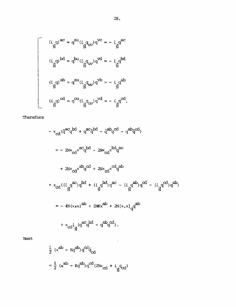
ab ab a b - = ~ ( n & - K q ) K + (n -Kq )vcNC.

Swmary : We have

ab ab - 1/2 + (X - ~ q ) V ~ N ~ O / q / . The final point is to note that

L (nab - Kqab) 3

acbd a b c d = L,(xcd(q q - q q ) )

N

Since v$ = div $, it follows that q

acbd abcd xcdL,(q q - q q ) Q? lql

1/2

N

Observation:

the preceding considerations into account, we then find that

d 6L -- (t) = - dt 6v,b 6L (t)

6qab

iff

which is equivalent to the assertion of the theorem.

One can also arrive a t the constraint equations by d d i n g that V t,

relationships which should be expected to hold on purely formal grounds (due to

the absence of the corresponding velocities in the definition of L ) .

[Note: H e r e

6 L Ad - W e have 6N '

d - L (q,v;N + EN' ,8) de

- d L ( ~ . v : N + EN' ,8) - J, d&

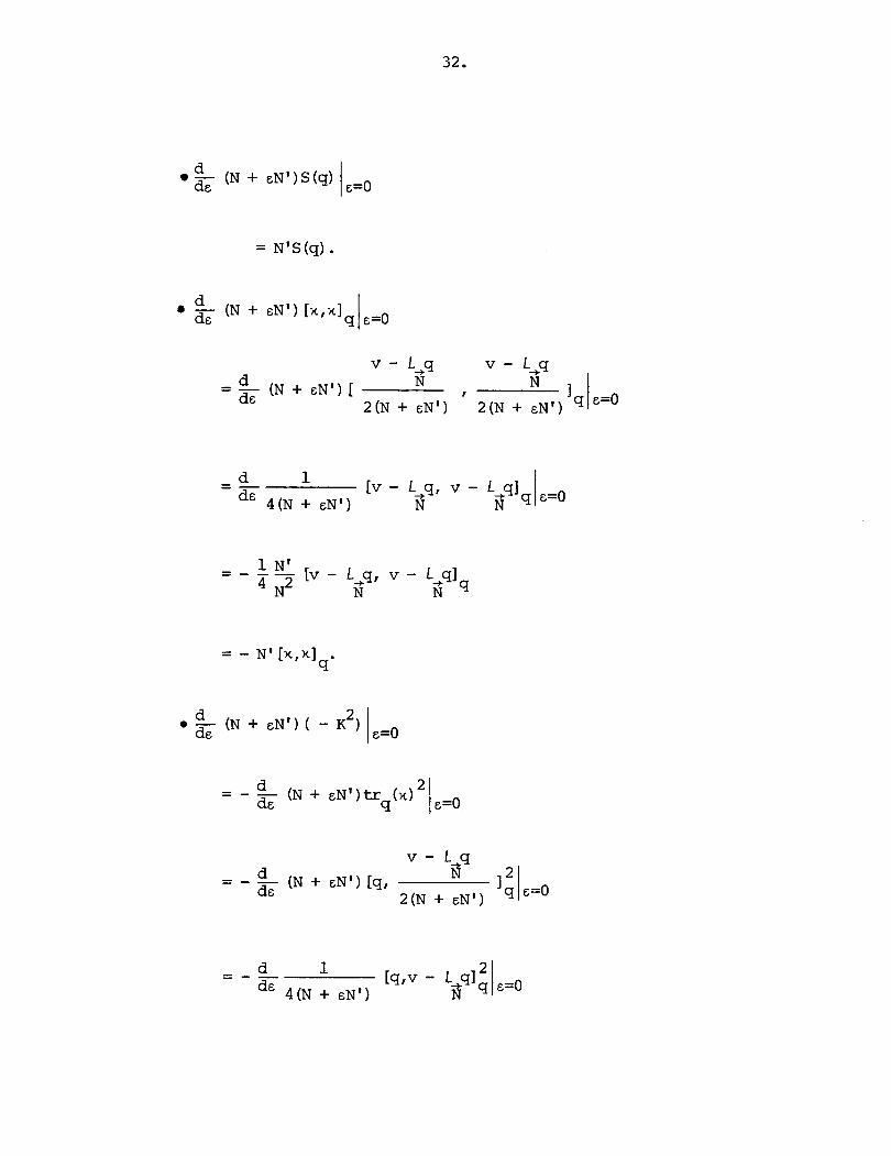
2 = N'K . Thus

and so

6L Ad - : We have 68

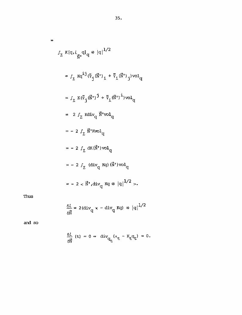
Thus

-- 6 L - 2(div x - divq Kg) o lq/ 1/2 63 9

and so

6 L - (t) = 0 - div (nt - KA) = 0. 68 %

Section 37: Dynamics Let M be a connected cm manifold of dimension n > 2.

Fix E (0 < E 5 00) and assume that

where C is ccanpact and orientable (hence dim C = n - 1).

S u p p e given a t r ip le (c+N 8 ) ( t F 1 - &,&I) (subject to the custdary t' t

stipulations) . 2 Definition: The ny-snentum of the theory is the path t - pt in Sd(E)

defined by the prescription

1/2 Pt = /%I 1

where

[Note: The mtivation lying behind the definition of n is the fact that t

Here p stands for n f & /q11'2 with n = n - Kq.]

One can then reformulate the results f r m the l a s t section along the

following lines.

Constraint Equations These are the relations

div pt = 0. 9t

molution Eauations These are the relations

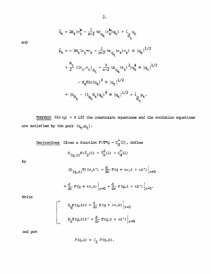
and

T'HEOmiI Ein (g) = 0 iff the constraint equations and the evolution equations

are satisfied by the pair (qt,pt) .

~erivatives Given a function F:T*Q + C: (z) , define

2 03

D (q,N

F:S~(E) x Sd(Z) -+ Cd(U

Write

Then

provided, of course, that the relevant functional derivatives exist.

[Note: Analogous conventions are used in other situations as well, e.g.,

1 i f instead F:T*Q + Ad (Z ) . I Define a function H:T*Q -r C: (z) by

2 , ( s ) - S(q)) @ 141 H(4.A) = ( [stsIq - 3 1/2 4

i f A = s' ~9 lq11/2 and for any £ € C ~ ( Z ) , put

and

So, as a corollary,

and

1 Define a function I:T*Q +. nd(z) by

I ( ~ , A ) = - 2div A. 9

1 Each XCV ( 2 ) thus gives rise to a map IX:T*Q +. C: (z) , viz.

Let

[Note: Recall that

# L# = LXs D lq11/2 + sU @ (div X) ~cJ/~/~.] q

Heuristics To see the origin of the preceding definitions, consider the

fiber derivative of L :

Then

[Note: Keep in mind that

Let

on T*Q correspnding to ff is characterized by the condition f IX

and can be represented in t m of functional derivatives:

Now specialize and take f = NtI X = 8tt. Replacing ( q , ~ ) by (%,pt) I

the evolution equations state that

Otherwise said: The curve

is an integral curve for Z

%f8t

Definition: Le t t -+ f ( t ) be a path in c ~ ~ ( z ) (or c ~ ~ ( z ) ) and let t -r ~ ( t )

1 be a path in D (2) -- then

the evolution equations i f

[Note: Here t lies

Example: If Ein (g)

a curve t -+ (q (t) ,A (t) ) in T*Q is said to satisfy

in m e open intewal centered a t the origin.]

= 0, then the curve t -+ (qt,pt) satisfies the evolution

equations, where

JxMm under

we have

the conditions of the preceding definition, along (q (t) A (t) ) ,

or, in brief,

dH We shall first consider x:

But

Therefore

It resnains to deal with

or still,

or still,

or still,

+ 6 div ( 2 f ( s - - 1/2 q q n-2

Since

and

tr (HI = A £ , q f 9

matters reduce to

+ 6 div (2fs) PP l q 1 1 / 2 + 2[s,H 1 8 1q11/2 q q f q

or still,

6 div (2fs) O lq/1/2 + 2[s,Hflq d /q/1/2. q q

[Start by writing

- 6 div (fs) = $ (div (fs) ), q q q

-a-b = v v (£slab

ab = (" );a;b

ab = (f sab + f s )

;a ;a ;b

= f s a b + f sab+ (£SF) ;a;b ;a ;b ,a ;b

= [ s ,Hf Iq + f

But

On the other hand,

-a 2 s) = V (f div s), q

2 = %(f div s ) ~ q

2 = (f div s ) ~

q ;a

2 2 = (f ) (div s) a + f (div s) a

;a q q ;a

Theref ore

1 2 6 div (fs) = - [stHfIq + - 6 (f div s) . ] q q f q q

Accordingly,

1 2 = - 6 (2f div s) @ lql 1/2

f q q

- 1 2 - - - 6 (f ( - 2div A ) ) f q q

dH This establishes the formula for

dI 1 Turning to f ix ~ € 0 ( 2 ) -- then

dI The formula for =thus follows, Y being arbitrary.

[Note: Integration by parts has been used several times and can be justified

in the usual way. ]

Poisson Brackets Given functions FIIF2 :T*Q + C; ( 2 ) , put

and let

be the corresponding hamiltonian vector fields:

Then the Poisson bracket of FlIF2 is the function

defined by the rule

Therefore

[Note: Tacitly, it is a s s d that the functional derivatives exist.]

LEMM24 Let F :T*Q + C: ( 2 ) -- then, in the presence of the evolution equations,

along (q(t) t A ( t ) 1 , we have

+ 1, W ( [X1rX21 r 1 )

[Fix a p i n t (qo,li0) and take f 2 in cZO(X). Choose paths t - f 2 ( t ) in

C- (x) and t -+ X 2 ( t ) in ~ ' ( 2 ) such that f2(0) = f2 , ~ ~ ( 0 ) = X2. L e t t -+ (q( t ) ,A( t ) ) 7 0

be the curve in T*Q satisfying the evolution equations subject to (q (0) ,A (0) ) =

(qo,no) -- then along (q( t ) ,A(t) ) , we h v e

And (cf. infra)

Setting t = 0 completes the proof when f2 is strictly positive. Assume now that

f2 is arbitrary. Fix C > O:f2 + c€C~~(Z) -- then

or still,

[Note: There are results in PDE theory that guarantee existence ( a r d

uniqueness) of solutions to the evolution equations, a fact which was taken for

granted in the above. This accounts for the initial restriction on f2.]

Details At a pint (q,~) ,

2 f2div s)vol q

div s)vol 4

= S, ev(fl(grad f - f2(grad f ) , 9 2 9 1

Scholium: The following formulas are special cases

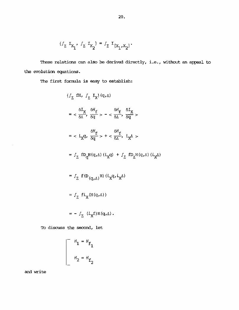
These relations can also be derived directly, i.e., without an appeal to

the evolution equations.

The first formula is easy to establish:

To discuss the second, let

and write

Then

a b abc + 2 J, f l ( v v f 2 - q v Vcf2) (s& -

a b a b = 2 lz l f lV v f 2 - f2v v "Is&vo~

q

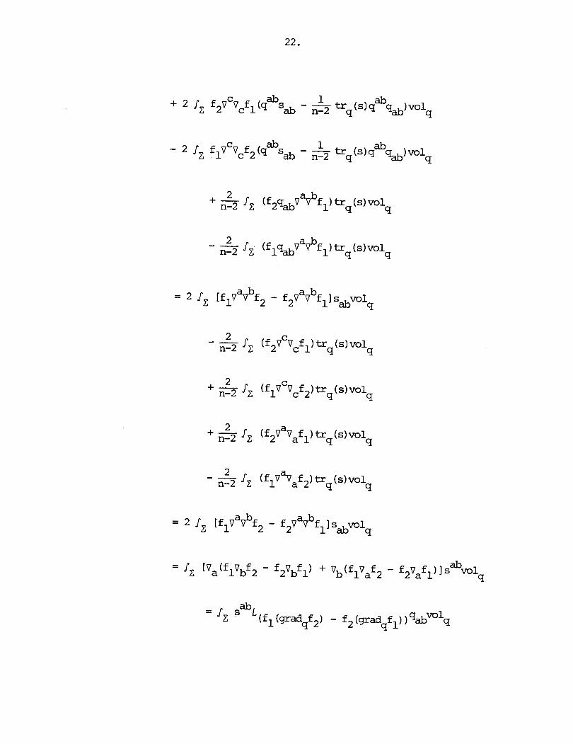
= q vol (fl(gradqf2) - f2(grad q f 1 ) ) ab q

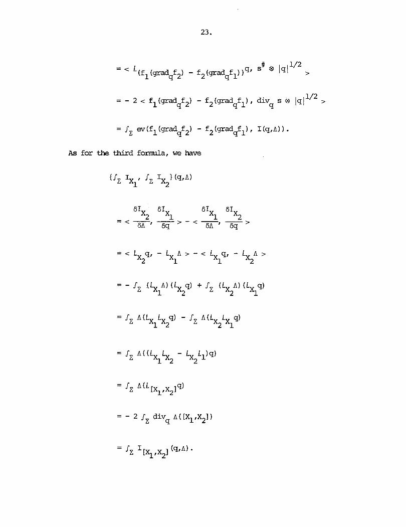
1/2 = - 2 < fl(grad f ) - f2(grad f ) , div S P P lq/ > 9 2 q 1 9:

As for the third formla, we have

Remark: The se t whose el-ts are the ff is a vector space over R f , X -

but it is not closed under the Poisson bracket operation since

and the vector field

depends on q. On the other hand, the se t whose elemnts are the 1, is a vector

space over R - which is closed under the

A

Poisson bracket operation:

So, in view of the Jacobi identity

it is a Lie algebra over R. - The arrow X + ix is thus a hom4norphism of L i e

algebras.

L e t

I- Co% = { ( q , A ) €T*Q:H ( q , A ) = 0)

I (3% = { ( q , A ) CT*Q:I ( q , A ) = 0 ) . -

Then

Con = ConH17Con,,cT*Q Q

is called the physical phase space of the theory,

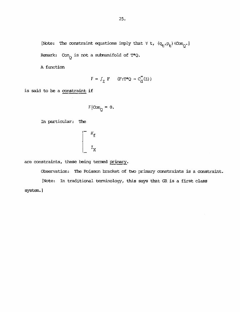
[Note: The constraint equations imply that V t, (%,pt) Con . 1 Q

Rgnark: Con is not a suhnanifold of T*Q. Q

A function

F = Jz F (F:T*Q + c ~ ( c ) )

is said to be a constraint i f

In particular: The

are constraints, these being termed primary.

Observation: The Poisson bracket of tsm primary constraints is a constraint.

[Note: In traditional terminology, this says that GR is a f i r s t class

system. 1

Section 38: Causality In this section we s h a l l provide a proofless

sumnary of the relevant facts.

Let M be a connected cm manifold of dimension n > 2.

Rappel: If M is noncmpact or i f M is campact and has zero Euler

characteristic, then %,n-l is not empty.

Asswe henceforth that M is nonccanpact. Fix g€MII n-l -- then the pair

(M,g) is said ~ be a spacetime i f M is orientable and t ime orientable (i.e. ,

admits a timelike vector f ie ld) .

Remark: The tangent space TJ4 a t a given x€M is R"~-'. - Therefore a

vector X€TxM is timelike i f gx(X,X) s 0, lightlike i f gx(X,X) = 0, and spacelike

i f gx (X,X) > 0. The carrplement in TxM of the closure of the spacelike points

has camponents ("timecones") and there is no intrinsic way to distinguish

them. If one of these cones is singled out and called the future cone V+ (x) ,

then TxM is said to he time oriented. A timelike or lightlike vector in or on

V+(x) is said to be future directed. The other cone is denoted by V - (x) . A

timelike or lightlike vector in or on V - (x) is said to be past directed.

[Note: If T is a &like vector field, then T$1 can be time oriented

by specifying the time cone containing Tx. 1

Assume henceforth that (M,g) is a spacetime.

(gl)x(X,X) = 0 i f f ( g 2 ) x ( ~ , ~ ) = 0.

Then

A curve i n M is timelike, lightlike, or spacelike i f its tangent vectors

are timelike, lightlike, or spacelike.

A curve in M is causal i f its tangent vectors are timelike or lightlike.

A causal curve is future directed (past directed) i f its tangent vectors have

this property.

A future directed causal curve y:I -+M is said to have a future endpoint

(past endpoint) i f y( t ) converges to some point i n M as t .f sup I (t C inf I) . A past directed causal curve y:I -+ M is said to have a past endpoint

(future endpoint) i f y ( t ) converges to scane point i n M as t .f sup I (t J- in£ I) . A future (past) directed causal curve y is said to start a t a point pEM

provided that p is the past (future) endpoint of y.

A future (past) directed causal curve y is said to be future (past)

inextendible i f it possesses no future (past) endpoint.

Notation: V p,q in M,

I- p << q: 3 a future directed timelike curve f r m p to q.

/ - p < q: 3 a future directed causal curve £ran p to q.

[Note: It may or may not be the case that p << p but i t 's always true

that p c p (conventionally, a constant curve is lightlike and both future and

past directed) . I

Definition: The chronological future of p is

1+(p) = {q:p << ql

and the causal future of r, is

The chronological past of p is

and the causal past of p is

J-(P) = {q:q < PI.

[Note: For a nonanpty subset ScM, the sets I' (S) , J' (S) are defined

analogously. E.g. : I+@) = {q:p << q (3 pCS) I and J+(s) = {q:p c q (3 pCS) 1 . + Obviously, I (S) = u and J+(s) = u J + ( ~ ) . Furthennore, J+(S)SUI+(S) .I

PES PES

LEWlA If x << y and y c z or i f x c y and y < c z, then x < < z.

Application: W e have

+ + + + I+(s) = I ( I S ) = I ( J S )

+ + + + + = J (I S)CJ (J S) = J (S).

LENMA If p << q, then 3 neighborhoods N of p and N of q such t h a t P q

I p1 << q'.

+ Application: V p a , I (p) is open.

Topological Properties V p€M,

+ + 1. int I (p) = I (p);

+ + 3. fr I (p) = {x:xfr: (p) & I+(~)CI+(~)};

+ + 4. int J (p) = I (p) ;

5. J+ CI+ (p) . +

Remark: In general, J (p) is not closed, hence may very well be a proper

subset of I+ (p) .

I - + +

future distinguishing if x # y * I (x) f I (Y)

I past distinguishing if x # y ;. I- (x) it I- (y) . -

[Note: Call (M,g) distinguishing if it is both future and past distinguishing.]

Let (M, g) , (MI , g ' ) be spacetimes. Suppose that f :M + Y' is a diff eamrphism -- then f is said to be a chronal isomrphisn provided

x << y - f(x) << f (y).

THEOREM If (~,g) and (M',gV) are distinguishing and if f:M -+ MI is a

chronal i~am~rphism, then f is a conformal iscanetry.

[Note: Spelled out, 3 CC;~ (M) : V x€M,

thus

Given p,q€M, put

Let S be a nonempty subset of M -- then S is causally convex if V p,qcS,

[PI ql cs

Definition: A spacetime (M,g) is said to be strongly causal if each x€M

has a basis of open neighborhoods consisting of causally convex sets.

[Note: A strongly causal spacetime is necessarily distinguishing.]

FPCr Suplase that (M,g) is strongly causal -- then the I+(~) n1- (q)

(p,q€M) are a basis for the topology on M.

A time function is a surjective cW function z:M -+ R - whose gradient grad z is timelike.

Definition: A spacetime (M,g) is said to be stably causal if it admits

a time function z:M -+ R. - FACT Every stably causal spacetime is strongly causal.

Definition: A spacetime (M,g) is said to be globally hyperbolic if it is

strongly causal and V p,qEM, [p,ql is compact.

+ LENMA If (M,g) is globally hyperbolic, then V p, J (p) is closed.

[Note: Mre generally, K cc~npact E. J (K) closed. 1

Example: Rl, n-1 is globally hyperbolic but R 1 ,n-1 - - - (0) is not.

FACX Let (M,g) , (&I ,g' ) be distinguishing chronally i~~~ll~rphic spacetimes --

then ( ~ , g ) is globally hyperbolic i f f (MI ,g ' is globally hyperbolic.

R-k: If (M, g) is globally hyperbolic, then so is (MIcpg) (cp €cCO (11) .

On the other hand, i f &g) & ( ~ , g ) are globally hyperbolic and i f the identity

map is a chronal is~~~~]rphi.sm, then g = cpg' for SCEE cp€cW (M) . 70

L e t (M,g) be a spacetime. Suppose that S is a nonempty subset of M -- +

then the future domain of dependence D (S) of S is the set of a l l points pfM

such that every past inextendible causal curve starting a t p meets S.

[Note: The definition of D- (s) is dual. The union D (S) = D+ ( s ) UD- (s)

is the damain of dependence of S.1

U3MA If S is a closed achronal subset of M, then int D ( S ) , i f nongnpty,

is globally hyperbolic.

[Note: S is achronal provided S ~ I ' (S) = @.'I

Definition: L e t (M,g) be a spacetime -- then a Cauchy hypersurface is

a closed achronal hypersurface ZcM with the property that D ( Z ) = M, hence is met

exactly once by every inextendible timelike curve in M.

[Note: A hypersurface per se is an embedded connected suhnanifold of

dimension n - 1. I 1 , n-1 Example: In R , the hyperplanes xo = constant are Cauchy hypersurfaces.

FACT - If Z1 and Z2 are Cauchy hypersurfaces in !A, then Z1 and C2 are

dif fecxmrphic.

In view of the preceding letma, i f (Mlg) admits a Cauchy hypersurface,

then (M,g) is globally hyperbolic. The converse is also true: Every globally

hyperbolic spacetime admits a Cauchy hypersurface but one can say considerably

mre than this.

+ FACT A spacelike Cauchy hypersurface Z is acausal, i.e., ZnJ-( ,z) = a.

SmCrClRE THM)REEt Suppose that (M,g) is globally hyperbolic -- then

there exists a connected (n-1)-dimensional manifold Z and a diffecmorphisn

Y : R x I: -t M such that V t, I: = Y ( { t) x 2) is a spacelike Cauchy hypersurf ace - t

in M, hence

Addenda

1. The spacelike leaves Xt of the foliation figuring in the theorem

-1 are the level hypersurfaces of a time function z , i.e., V t, Zt = T (t).

2. The vector f ie ld grad z is past directed but possibly inccmplete.

To remedy th is technicality, l e t

- grad T xT - l brad T I l

H e r e the norm is taken relative to sane ccanplete r i g ~ n n i a n metric, thus X is T

a canplete vector field. Put I: = (0) and define a diff-rphim 0:Y -t R - x Z

where p(p) is the unique point of 2 crossed by the maximal integral cuwe of

xz through p. Let P= 6' -- then v t,

3. Put

Given XCZ, let

yx(t) = y (t,x)

!I'hen yx:R + M is an integral curve for - a It is timelike and az'

t c t' J yx(t) c< y x ( t l ) .

Furthermore, ?- is parallel to grad T: V t, az

So V t, yx (t) lies on the trajectory of XT containing x.

4. If L CM is a Cauchy hypersurface, then y (t) intersects ZO exactly 0 X

once a t the parameter value tz (x) . The function tz :Z + R is cm and - 0 0

ZO = { Y (tZ (x) ,x) : X€Z ) . In addition, i f Z , Z are Cauchy hypersurfaces , then 0

1 2

the map zl + Z2 which sends Y (5 (XI ,x) to Y (5 (x) ,XI is a diffecmorphisn. 1 2

5. Since T = t 0 @, it follows that

Therefore

6 . Let q ( t ) be the r i m i a n structure on Z determined by pulling

back g via the arrow

yt i 2 % {t) x Z

t -* Zt - M.

Put

Define gTglf n-l (per R x 2) by the prescription

Then

gT = I*g.

But this implies that

Ein (g,) = Y*Ein(g) ,

thus the vanishing of Ein (gT) is equivalent to the vanishing of Ein (g) . Terminology Let (F4,g) be a globally hyperbolic spacetime.

* M is spatially canpact if its Cauchy hypersurfaces are ccanpact.

M is spatially noncolrrq?act if its Cauchy hypersurfaces are noncanpact.

FACT Suppse that (M,g) is globally hyperbolic. Let Z c M be a closed

achronal hypersurface. Assume: r, is carpact -- then Z is a Cauchy hypersurface.

LETN9 The Cauchy hypersurfaces in a globally hyperbolic spacetime are

orientable.

Let

~ ~ = I - E , E [ X Z (OCES-),

where Z is orientable (hence dim Z = n - 1). Suppose given a triple (qt,~t,$)

satisfying the usual conditions and let g be the element of ?41,n-l determined

thereby (for this, it is not necessary to assume that 2: is canpact) -- then, in general, the pair (Pl,g) is not globally hyperbolic.

[Note: The spacetime (M,g) is, however, stably causal. Thus take for

z the projection (t,x) -+ t -- then

grad t = (dt) #

g(qrad t, grad t) = - 1 - < 0. N

2

Therefore grad t is timelike. 1

OAssume that 3 a complete qEQ and positive constants A > 0, B > 0:

.Assume that 3 positive constants C > 0, D > 0: V t & \J' xCZ:

Assume that 3 a positive constant K > 0: V t,

-+ -+ QJtfNt) 5 K.

FACT Under these conditions, (M,g) is globally hyperbolic and the slices -

It) x 2 are spacelike Cauchy hypersurfaces.

[Note: There is also a converse: Make the same assumptions on the data

except for the ccsnpleteness of q, form (M,g), and suppse that it is globally

hyperbolic -- then q is necessarily cqlete.]

Example: When fi = 0 and q and N are independent of t, g is said to be

static. So, in this situation, (M,g) is globally hyperbolic if (Z,q) is q l e t e

and N is bounded above and below on C (matters being autmatic if Z is ccarrpact).

Section 39: The Standard Setup The pint here is to initiate the

transition £ran a theory based on metrics to a theory based on forms.

LEMMA Every connected orientable 3-manifold Z is parallelizable.

[For the proof, it will be convenient to admit manifolds with boundary.

Thus let -

I wl (z) = lSt ~tiefel-~hitney class

w2 (Z) = 2nd Stiefel--Whitey class. I - Then z is parallelizable provided wl(Z) = 0 = w2(z). But wl(.Z) = 0 is aukmatic

(Z being orientable) . 2

Case 1: Z conpact and aZ = 8. Proof: wl(Z) = 0 - w2(Z) = wl(" = 0

(Wu relations) . Case 2: Z ccanpact and ax # 8. Proof: Consider the double of Z and

apply Case 1.

Case 3: Z nonccmpact and aZ = j3. Pmof: Let a€H2(Z:Z/2Z) - - be

arbitrary -- then a is represented by a compact surface S + C (Thm), hence

Case 4: z noncampct and ax f j3. Proof: consider Z - a2 and apply Case 3.1

Take n 7 3 and let Z be a connected ccanpact (n-1)-dimensional orientable

cm manifold.

Assumption Z is parallelizable.

Put

M = R x Z . - Then M is also parallelizable.

Notation: Indices a,b,c run £ran 1 to n - 1.

Let E1,-.-,En-l be time dependent vector fields on r, such that tl t,

is a basis for ~'(2). Canplete this to a basis

for D' (MI . Construction Let q(t) be the element of Q determined by stipulating

that the Ea(t) are to be an orthonormal frame -- then the prescription

defines an elanent of Mlfn - -

Rgnark: This procedure gives rise to a certain class of spacetimes

(M, g) (Eo is a timelike vector field) . In general, however, if g $ I , n-l is

arbitrary, then one has no guarantee that g Z is randegenerate, let alone

spacelike. On the other hand, there is a gauge-theoretic ambiguity: Distinct E

m y lead to the sam g.

[Note: While not necessarily globally hyperbolic, the spacetime (M,g)

is at least stably causal (the projection (t,x) -+ t is a time function) .I

In view of the definitions, 3 cm functions N and E? on !?I such that

a= NEo + %. a t

[Note: N has constant sign, i.e., N is s t r i c t ly positive (or s t r ic t ly

negative) . I

~erminology: N is called the lapse and 8 = N ~ E ~ is called the shift .

Reality Check Suppose given a t r ip le ( q , , ~ ~ , 8 ~ ) satisfying the usual

conditions. Fix t i m e dependent vector f ields El, ..., EnV1 on Z which a t each

t constitute an orthonormal frame for q (t) . Take

Then

which is in agreement with the earlier considerations.

Let it:z% - t M k thembedding (zt= {t) x 2). Zt

0 Notation: Given T€D (M) , put q

We have - T = i * L

t a/atT-

[In fact,

where 4 is the flow attached to s. Therefore

4;T - T - - i* lim

t s - t O S

Example: By construction,

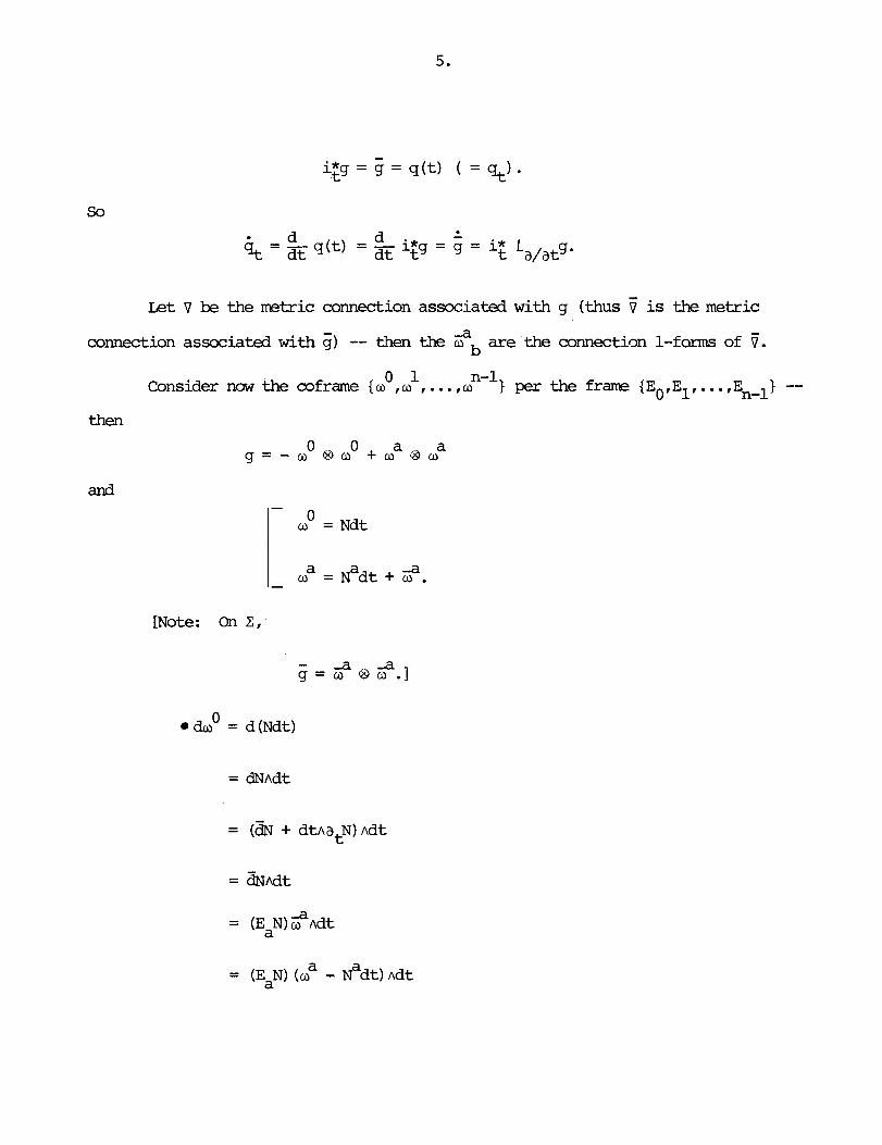
L e t V be the metric connection associated w i t h g ( t h u s 7 is the metric

connection associated w i t h g) -- then the ijab are the connection 1-£0- of i.

0 1 C o n s i d e r now the coframe { o , o , . . . , on-'] per the £ram {EO ,El, . . . , En-'} --

then

0 a a g = - 0 O o O + o @ o

and

I - o a = N a d t + $ .

[Note: On 2 ,

. dao = d (Ndt)

= (a + dtnatN) ndt

= & ~ d t

= (EaN)$ndt

= (EaN) (oa - 8 d t ) n d t

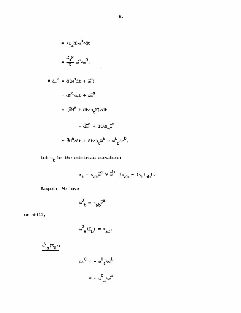
= (3 + dtAatN) A d t

L e t xt be the extrinsic curvature:

Rappe l : We have

or s t i l l ,

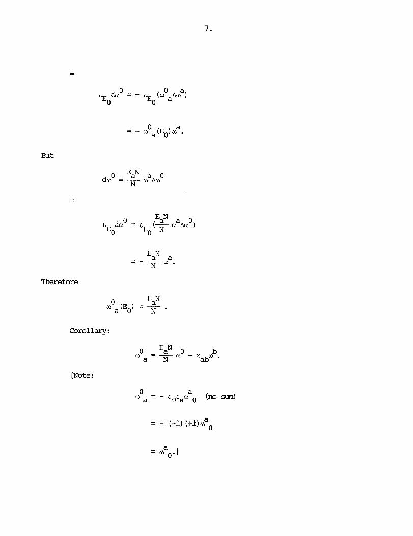
- a - - ooa (E,) 0 .

But

o *aN a o do = - N o Am

*

EaN a o L duo= (-ano) *o N

EaN a = - - N 0 .

Therefore

Corollary:

[Note :

8.

Rappel: We have

a w (Eo) :

or still,

*

But

and

[Note :

Remaxk:

- (3) -Nu&

'ab is symnetric while oh is antisynmetric.]

since g = za N 5, it follows that

- gab = ij, 'Eb' + 5 (Ea) .

Theref ore

Definition: The rotational parameter of the theory is the function

LEMMA W e have

[It is a question of explicating the relation

Write

Then

But

Theref ore

[Note: In terms of the extrinsic curvature,

Notation: Put

Then

Notation: Put

Then

LlW@ We have

[Consider the first relation. Thus

[Note:

and

Let p,v be indices that run bebeen 1 and n-1. Wrking locally, write

Then

To simplify this, w r i t e

Reality Check The claim is that

equals

or still,

a b =2Ne e x t y v a b '

On the other hand,

a b 2 i e e

P v

a b =2Ne e x t p V a b '

But

Now use the foil-g relations

to get

Therefore

a b a b 1 + 2 = (VbNa)e e + (Ta%)e ,e w v

a b = (TbNa) ea eb + (VaNb) e e

II. v P v *

1 N.B. -- V XED (Z) ,

-b

[Note: The verification is an exercise in the definitions and will be

detailed later on.]

Section 40: Isolating the - Lagrangian The assumptions and notation

are those of the standard setup.

Rappel :

i j eij = * (0 no ) (i, j = O , l , . . . rn-l) .

[Note: oil is an (n-2)-fonn and the Hodge star is taken per

Consider

Write

. . [Note: Obviously, eiJ = - el1. In addition,

Since b

'0a = d%a + O b A W a'

it follows that

O b a a O b n-2 Oa = ( - w b ~ e - a b ~ e ) nooa + (-1) e AdaOa

Therefore

i j e naij = Oa ab 0

2d(6+,a~0 + 20 AW

But

and

Remark: The explanation for singling out the term

is the fact that

the overbar standing for pullback

Notation: Put

[Note: The Hodge star is taken per

but there is a caveat: G& is not equal to i;€Iab (which, in fact, is identically

zero (cf . infra) ) .I

Proceeding formally, set aside the differential

and ignore all issues of convergence -- then

Details To see the passage f r m

ab 0 i$,a/at[e - w AW b) - w ACO ) I a0 Oa Ob

recall f i r s t that coo = ~t ( L 0

= N), hence iza = N i X d t = 0. t t

Tkis sa id , write

Put

Then

And

[Note: To discuss the effect of canitting

£ram these considerations, observe that

It rmains to examine the integrand::

= - det 1 I *

But

Therefore

- - - det

Accordingly, at each instant of time,

2 = I Z N t (S(qt) + [ z , x ~ I % - Kt)v01 1

q t

which is in complete agreement with what has been established earlier.

Section 41: The Pbnentum Fonn The assumptions and notation are those

of the standard setup.

R e c a l l that the mmentum of the theory is the path t -+ pt 2 i n Sd (2) defined

by the prescription

where

In this section, we shall show that pt is closely related to a certain element

Notation: L e t

Definition: The m~~nentum form of the theory is the path t -+ Gt i n

dn-2 0 12 ; T1 (Z ) ) defined by the prescription

LEMMA W e have

[To begin w i t h ,

But

Therefore

Consider naw

Write

Then

and

afb: In this case, -

By definition,

where

But

Irdeed,

Let

Then

LEMMA We have

[Write

Application:

[In fact,

Section 42: Elimination of the -Metric The assuqtions and notation

are those of the standard setup.

Then the dynamics can be formulated in terms of (Zt,6t) a s opposed to (%,pt) ,

i.e., there are again constraint equations and evolution equations. While this

approach does not lead to new results, the methods are instructive, thus are

mrth examining.

L e t Q be the set of ordered coframes on Z -- then each ~ F Q gives rise to - - a riemannian structure qCQ, viz.

a a q = o @ o .

Conversely, each qEQ gives rise to a coframe &Q - which, however, is only determined

up to a local rotation.

[Note: A t this pint, M does not play a role, hence the absence of overbars

in the notation.]

Put

Observation: There is a canonical pairing < , >

[Note: EZplicated, on general grounds,

n-2 0 Consider T*Q = Q x A (Z iT1 (Z) ) -- then - -

The Canonical 1-Form 0 This is the map

defined by the prescription

The Canonical 2-Form Q This is the map

defined by the prescription

LEWA W e have

a = - do.

[In fact ,

Therefore 51 is exact and the pair (T*Q,Q) is a symplectic manifold. -

Suppose given a function f:T*Q -+ R. I -

*n-2 - : Write

n-2 0 for that element of A (Z ; T1 (2) ) characterized by the relation

1 n_ : Write

1 1 for that elanent of A (b;TO(z)) characterized by the relation

Sf 6f + -+ [Note: Bath - and d e p d on (a, p) , thus 6; SP

Definition: The hamiltonian vector field

Xf:T*Q - + TT*O -

attached to f is defined by

To justify the terminology, let X be any vector f ie ld on T*Q. Suppose that - -+ +-

X(w,p) = (2 ,St) -- ,then

6f -+ -+ 6f = i2 (, Ap' - o'n - -) 6~ 6':

Example: Each coframe determines by duality a f r m 3, thus

This said, let

Then it is clear that

Definition: The configuration space of the theory is Q, - the velocity phase

space of the theory is TQ, - and the r r ~ ~ n e n t u m phase space of the theory is T*Q. - + +

Elements of Q are denoted by z, elments of TQ are denoted by (o,v) , and - - + +

elements of T*Q are denoted by (wfp) . - The theory carries three external variables, namely

where Ypb€cm(Z) and Ypb = - Wba.

+ -+ Given ( ~ , v ; N , ~ , w ) , put

Definition: The lagrangian of the theory is the function

defined by the rule

+ + L ( ~ , v ; N , ~ , w )

[Note: A s usual, the (n-l)~ab are the curvature £0- of the m t r i c

connection vq associated with q and, of course, the Hodge star is taken per q. I

L e t

Then, in order to transfer the theory from TQ to T*Q, it w i l l be necessary to - - calculate the functional derivative

n-2 0 which, a p r i o r i , is anelement of A (Z;T1(Z)):

Notation: L e t

[Note : Therefore

LEMMA We have

[TO faci l i ta te the computation, "variational notation" w i l l be employed,

i. e. , we shall replace the symbol vat by 6va and abbreviate D a to -- then v

a = 6v ma.]

[~ote: This result is the reason for the "1/2" prefacing the integral Iz L.1

6L is widely Ranark: The method employed abave for the calculation of - sva

applicable and will be used without mment whenwer it is convenient to do so.

[Note: The interior derivative is not a participant, hence the possibility

of misinterpretation is minimal. I

Consider now the fiber derivative of L:

Then

To simpli£y th is , write

L e t

Then

Theref ore

On the other hand,

Motivated by these considerations, let

be the function defined by the prescription

[Note: Here the external variable N is unrestricted, i.e., N can be any

element of cm (2 ) . I Definition: The physical phase space of the theory (a.k.a. the constraint

surface of the theory) is the subset Con of T*Q whose elements are the points Q - -

+ + (o,p) such that simultaneously

6 ff The calculation of - is trivial. Thus define m

E:T*Q + A"-$ -

Then

6H , observe that Turning to - &b

Therefore

There remains the determination of - 6H To this end, fix a -- then b '

Write

But

And

c ~ c ~ % ~ ~ = d - 6 ~ ~ ~ d ~ ~ .

Since

f, d ( 6 ~ ~ ~ p ~ ) = 0,

it follows that

[Note: The intqal

can be rewritten as

Here

is defined by

-+ + Scholim: Con is the subset of T*Q consisting of those pairs (o,p) such Q -

that

subject to

Definition: -f +

The ADI sector of T*Q consists of the pairs (o,p) for which -

6 ff In the ADM sector of T*Q, the functional derivative - - can be expressed in 6Na

terms of the R-linear - operator

To see this, recall that

And

Therefore

But

Since n = d h M > 2, the vanishing of Ein(g) is equivalent t o the vanishing

of Ric(g) and for the lat ter , conditions have been given in terms of the path

t + (%,xt) in 'IQ or the path t + (q,,pt) in T*Q. H a u w e r , one can also work

instead w i t h the path t + (Zt,$ in T*Q, there being, as always, t w o aspects t o - the analysis: Constraints (i.e., the Goi = 0 equations) and evolution (i.e., the

Gab = 0 equations). In the next section, we shall t rea t the constraints and, in

the section aftex that, evolution.

Rappel: The qnmetry of the extrinsic curvature implies that the cmponents

pa of the mxentum form 6 satisfy the constraint t

i.e., the path t + (<,4) l ies in the ADM sector of T*Q. -

Section 43: Constraints in the Cofrane Picture The assumptions and notation

are those of the standard setup.

Rappel: 'd t,

[Since

-b * P 6 Y- = %(Pat*'") - n-2 t *I

we have

- P 6 -b -a - - n-2 t *%(pa,*zb) - g t ( p a I * ~ )qt(pbt*w - P26 6

(n-2) 2 t a b a b

gt [Note: T stands for \J .]

It suffices to deal w i t h

- v - d Pa

as opposed to

[Note: B e a r inmind that

This said,

Pa = (Xt - Kt%)**%

U s i n g the definitions, one finds that

- V d (ut - Kt%) &A*%

- vol (see below)

- - "av0'%-

On the other hand,

= 0.

Therefore

- - - Eoavol st'

Details The claim is that

a relation which I s a special case of the following generalities. Thus let

a b O T = T d CD o EV2(Z) .

1 Fix a VEcon TX - then b' XED (Z) ,

But

- - < Ec.d V Trs >.

Theref ore

[Note: These considerations apply in particular to the choices

Section 44: Evolution in the Cofram Picture The assumptions and notation

are those of the standard setup.

Rappel :

a b = I o Apa + e b o Apa + f2 NE, = 3

where

There are rn t m central objectives:

W e shall start with a, which turns out to be the easier of the tm. 'Pa

Obviously

6U - -- a b 6 L+o + Wabw + - iz NE]. N 6pa

Granted I and 11, it follows that

Ad I: Consider

But

a b = 2q(pb,xw

thereby establishing I.

Ad 11:

- P a - - - q(6pa,*o ) V O ~ n-2 q

- P a - - - w Asp,. n-2

Smmary: We have

6H is m e difficult. However, it is at least clear that The calculation of 7 60

[Note: Pinned down,

We have

[There are two points:

1. vol = 1

E bl bn-l

W A ... A a q (n-1) ! bl.. . bn-l

Accordingly,

Then

b b = fja* ( w Apc) A m 1 + * (o A p ) A 6 vol

9 c a q'

Therefore

c b (a A%) A6a* (0 Apt)

b - *(a A P ~ ) ~ 6 ~ ~ 0 1 ) . 9

But

b 6,(*(~ ApC) AVO^

'4

b = 6a(a Apt)

b = €iaa Ap,.

So, in view of the lemna, it fo l laws that

c b (w Apb) "6,* ( 0 Apt)

b b = q (pb, *aC) (6 a w A p c - * (w Apt) 6wa~*wa)

Now add I and I1 to get:

or still,

or still,

LZNMA We have

b c a a b c (a A o ) = 6o A* ( w A o A w ) .

[In fact,

b c &ja* (0 A w )

a a b c = 6 w ~ * ( w A o A o 1.1

Application:

b c a a b c Q A 6 1; (0 A o ) = So AQA* (o A o A o ) . bc a

Rappel: E%y definition,

is the Ricci 1-form hence

= S(q) .

[Note: There is an expansion

2 LEMMA Let aEA Z -- then

a b c a A * (o A o A m )

[For any index d between 1 and n-1,

a b c d q(aA*(w ~o ACO ) ,*w ) V D ~ (2

a b c d = aA* (a ~w Aw ) A**w

n a b c d = (-1) a h (w Aw Aw ) Aw

d a b c = w AaA*(o Aw Aw )

d a b c = q(w Aa,w Aw Aw )vol q

- a b c - t (a AW Am )m1 w Aa q

- a b c - LaL d (w Ao Aw )vol

w q '

an expression which surely vanishes i f d # a,b,c. Therefore

a b c a b c an* (w AO Aw = Ca*w + 90 + Cc*w .

H e r e -

a b c a Ca = q ( a ~ * ( o ~w ho ),*a )

But

a b c a . C a ~ l = q (an* (a nw A o ) , *o ) vol

q q

- a b c - Lat a

(w A 0 A 0 )vol o g.

Application:

a b c %A* (a A 0 A 0 )

Therefore

The final point is the analysis of

or, as is preferable, of

Put

Then the ebc are the ccmponents of an elanent

thus

and

Rappel: We have

But then

b c 6,QhcA*(w Aw )

= 6,SAB bc

) n P = 6 a ( s + w"

bc d bc A O ~ ~9~ + ~ A 6 ~ a = d t j a y x : A e + S a w

bc = d(6aWoc~9

d bc + 6a%

ndebc + 6awod"~d nobc + C a c

bc = d ( % s ~ e 1

bc dc + 6 a y x : ~ d ~ + B a s A u d

The differential

integrates to zero, hence can be set aside. Write

Then

But

C dab = - aib Aw C

Qnit the differential

b d ( 6a0 A* (dNA%) 1

which, of course, will not contribute - then

LEMMA We have

vq a d *(dNnwa) = *(vadN - (d$I)w ) .

[Write

C dN = Ncw (Nc = q(dN,wC)).

Then

But

a c b - w A* (NCo AW ) . b

Make the obvious cancellation -- then

vq d *(&A%)

c a b a = mcA* (o Ao ) + NcA ( - ocbA* (o Ao ) )

c a %A* (W AW. )

c a = q (dNc I ob) obA* (o Ao )

= q(mcIob) (-I)"-~* (oCAma) Amb

b a = ( - l ) "Ncn ( -1) n-2* ( L ( a A 0 ) )

b

c b a c a b = Nc*(q(o - q ( a b ~ W ) W )

c b a c a b = *(Ncq(o ,.a ) a - N c q ( ~ 10 1.

Hcwever, by definition,

b c % = V r n = o @ ( % - a N )

b c

=a

c b vadN = < Eat% - W bNc > W

b c b = < Ea,dNb> o - N C < E a , W b > W

a c c a b = q ( m c t ~ ) a - N c q ( w ) W

In addition,

Putting everything together then leads to the conclusion that, mdulo an

exact f o m ,

b c a a - 6 %A* (o AW ) = - 6 0 A*(', dN - (dqN)o ) . 2 a a

S u m w r y : We have

Constraint Epations These are the relations

Evolution Euuations These are the relations

and

In the last section, we saw that

and

Therefore the constraint equations are equivalent to

Turning to the evolution equations, note that

which is precisely the functional derivative %- evaluate3 at ( , ; ,8 ,oab) . 6Pa t t t t

In view of this, the evolution equations thus say that

In other mrds: The curve

is an integral curve for the hamiltonian vector field

attached to ff (all data taken at t) .

MAIN THEOREM Suppose that the constraint equations and the evolution

equations are satisfied by the pair

[Note: It is this result which justifies the passage to the coframe picture.]

To prwe the theorem, it suffices to shw that if V b,

then

# 1/2 + ( - ( A Nt)%) 0 lqtl +L+pt* t g t NL

And for this, one can work locally.

Let p,v be indices that run between 1 and n-1.

[Note: Bear in mind that g and gt are one and the same. ]

UW7A We have

Str ic t ly speaking, n vol and n @ 1 qt 1 'I2 are different entities but t C L c

for the purposes a t hand, it is more convenient to use n+volrc . Agreeing to

denote it also by pt, the evolution equation

replaced throughout by

for fir is as abuve, the only change

LEMMA We have

[In fact,

The point now is to apply the lemm and replace & by its evolution equation, the claim being that the result is the evolution equation for bW.

t

The first item on the agenda is to check that there is no net contribution

£ran the rotational terms.

: The rotational contribution fran % is

or still,

But

So the t w o rotational terms do indeed cancel out.

Consider f i r s t

Since

we have

But there is mre, viz.

1 'V = N (-)tr (n )n vol t n-2 qt t t qt'

Thus

is accounted for. There remains

or still,

or still,

-a P -C V - 2Nt (o e a ~ ~ c ) *a ) e

or still,

To begin with,

- - - Nt - - 1 (nt) 2~ e e v vol 2 n-2 qt b b qt

This leaves

or still,

or still,

or still,

Here

And

-c v = - N ~ ~ ~ x I J . A * ~ e

- - - P v e e vol Nt%c c b qt

= - N ~ R ~ C ( E ~ , E J epCevbvol 9t

= - N t R k (e V ' a a C axp st

- - - ' R epcevbvol Nte be c v l p l %

= - N eP epl ev ev' t c c b bR vol

p ' v l %

PP' " I R W1 = - Nt% 9t

p ' v ' qt

PV = - NtR vol %-

Item:

(c - ( A N ~ ) ~ ) v o I . t % st'

For it is clear that

On the other hand,

which, in ccanplete analogy w i t h the discussion of Ric, reduces to

Item:

equals

i.e., equals

Therefore the issue is the equality of

and

Write

to get

Then

so what's left is the equality of

( L+ dxP~%) evb Nt

and

or, equivalently, that

To see this, take p = v (the general case is similar (because p pv = pvp)) --

Indeed, each term is an n-form while dim Z = n-1. Apply t : 53

The sum 1 + - - - + 6 is zero.

n-3 times 2 + 5 equals (-1)

n-3 i. e. , equals (-1) times

( f. dxpAdXp + d x p A ~ dxp) A t -b

Nt 3 t a".'

which is zero.

Therefore

Section 45: Camputation of the Poisson Brackets The assuntptions and

notation are those of the standard setup.

Given functions flIf2:TXQ - -, RI - let X1,X2 be the corresponding hamiltonian

vector fields -- then the Poisson bracket of flIf2 is the function

Ifl,f21:T*g -+ 5

defined by the rule

Therefore

[Note: Tacitly, it is assumed that the functional derivatives exist.]

Rappel :

where

Definition:

is the integrated diffeamrphism constraint;

is the integrated rotational constraint;

is the integrated hamiltonian constraint.

Therefore

and we have:

= ff (N grad N2 - N2 grad N1) D 1

Ranark: A constraint is a function f :T*Q -t R such that f 1 con = 0. - - a

primary. The foregoing relations then imply that the Poisson bracket of two

primary constraints i s a constraint.

Ad 1: We have

Therefore

Ranark: The canonical l e f t action of Diff Z on T*Q - is syrtplectic (i.e.,

'v' cp CDiff Z , cp-S2 = $2) and admits a rm~mentum map

1 J:T*Q - + H ~ ( D ( 2 ) ,R ) , -

which provides an interpretation of HD.

Ad 2: We have -

6HR (W) 6ffD ($ 6ffD ($1 tiffR (W) = fz 1 A A I -

66 6; sEf sf;

But

Therefore

L e t - -++ 1 c b P

2

%h(~t~) = [q(pbt*w )q(pct*~ ) - z]mlq

-+ + 1 E (alp) = - 2 S (q)vOlq.

- pot

Then

thus

kin: - We have

But

Therefore

- pot: W e have

it being clear that

6ffH (N) pot = 0.

Write

and hold the second term i n abeyance for the mment -- then

But

It remains to consider the contribution

Bearing in mind that this is a sum over the index a, replace 6a i n the earlier

analysis by Lj - then N

Therefore

Remark: The elments figuring i n the in-at& rotational constraint are

mth functions W: r, + - so (n-1) . Agreeing to view cW ( 2 ; - so (n-1) ) as a Lie algebra,

it follows that the a r m W + ffR(W) is a hcmmmrphism.

[Note: On the basis of Etepns 2, 4, and 5 , the integrated rotational constraints

are an ideal in the fu l l constraint algebra.]

= 0.

Proceeding, note that

b a

=Wavol = 0. a q

So now, a l l tbat's left is

- yP,."...i.,

b + VPbO **vadN.

W r i t e

Then

b c = NWa Ric 0 A*w b ac

But Ric is syrmretric and W is antiqmnetric, hence

Finally

Ad 6: W e have

Insert the explicit formulas for

Then, after cancellation, matters reduce to

which we claim is the same as

To see this, recall that

a b P q(Pb,*o )a - - aa = - 0 n-2 Oa'

But

Therefore

Reversing the roles of Nl and N2 then ccmpletes the verification. Pbving on,

write

Ic (NlvavbN2 - N2vavbNl) Wa"pb

Nm use the identity

1 valid for any XED (C) (cf infra) . Thus let

X = N1 grad N2 - N2 grad N1.

Then

a + <(N1 grad N2 - N2 grad Nl) w A%

=>

= H (N grad N2 - N2 grad N1) D 1

A s for w h a t remains, viz.

= det I I

[Note: In the AIM sector of T*Q, - the Poisson bracket

= det

- -

vbNl 'aN1

- 'bN2 'aN2 -

Details Here is the proof that V XEV'(L).

b a b ( v b P ) w = L,pa + w b ( X ) w .

1.e. :

Star t w i t h the RHS - then

a a (vxwa) (Y) = xu (Y) - w (VxY)

c a = ~~9 + X w

c a = & ( % I +Xwc'pb'.

Turning to the LHS,

Ox = Ea 8 (dXa + waCxc)

=>

a = ax"(%) + w c(%)~c=

Remrk: The relation

a b p w a w = - q(pb,*w )w + - Oa n-2

is really a definition, though, for consistency, one should check that

a b = w A* (w Aw ) Pa ob

or still,

Section 46: Field l?qyations Let M be a connected cm mifold of dimxsion n.

Assume: M is parallelizable.

Notation: co$ is the set of ordered cofrms on M.

n [Note: Each w = {wl,.. . ,a 1 in cofM gives rise to an el-t viz .

1 n Definition: Let o = {w ,..., w 1 be an elenent of oofM -- then a variation

of w is a curve - 1 n

E + U(E) = (w (E) ,..., w (E)) , where

i i i w (E) = w + ESW

and the 6wi~nk have mnpact support.

[Note: This usage of the symbol 6 conflicts with that used for the interior

derivative which, to eliminate any possibility of confusion, will be denoted in

this section by d*.]

Let F:cofM -+ V, where V is a vector space over R - - then by definition,

[Note: It is custorary to write SF instead of DwF(6w) and F instead of

F(w). This shorthand is canputationally convenient and normally should not lead

to misunderstandings. 1

In what follows, we shall use the abbreviation w + E ~ U to designate a

variation of w.

Rules

Suppose that a:cofM + A ~ M - then

6da = d6a.

[Note: Spelled out,

N.B. - 1. In general, 6 does not conmute w i t h the Hodge star:

2. In general, 6 does not cmnute w i t h the interior derivative:

6 o d * # d * 0 6.

Rappel :

On the other hand,

Rappel :

il.. .i i j

.ip 60 = 6. A t w 0

j

[In fact,

j = --?3L E ... E E ( 6w A (:p2 A j n ... A w )

(n-p) ! il ip il.. .ipjpljw2. . . jn

Example :

For another example, define

Then

TI-E computation of R . . miJ is irmediate: 1 3

k i j = 8w AR. . ~ 0 k.

13

Turning to the ccmputation of 6R. .Aeij, note first that 1 3

On the other hand,

And

i j d * ( w Aw )

But

Therefore

ij Since the exact term 652..A8 is dynamically irrelevant, the formalism dictates

1 3

that

To see the significance of this, write

Rick the Ricci 1-form. Accordingly, if we define the Einstein 1-form by

6 L then the vanishing of the --r; (k = l,...,n) is equivalent to the vanishing of 8w

where

One can also incorporate a comlogical constant A: Take

1 i j LA(w) = - R . .A0 - 2 17 g

and let

LA (u) = Jy LA (4 - k

Since 6~01 = 6w A*%, the foregoing analysis implies that

Exercise: Ccanpute % if L = 6w

Given a:cof + A ~ M , write M

Therefore

Remark :

= (-1) "-lt (W . ACX) A ~ w j 7

Thus

or still,

[We have

The $ are (n-1) -forms and the collection dl . . . ,J"> is called the current attached to the pair ( a , B) .

Consider the trace of the current attached to the pair (a, P) :

= * (pBA*a - (n-p) aA* 6)

Therefore 9, = 0 i f f n = 2p.

Observation:

Rappel: V ~EA'M,

1.e. :

Thus

= 0.

But then

J'I&] = 0,

SO in th is case,

let L:cofM + A%, where L depends on and dw:

1 n 1 n L = L(w ,... ,W ,dw I . . . ,dw ) .

Then

Here

Now rewrite 6~ as

Definition: w satisfies the field equations per L provided v i,

[Note: Formally, if L = L, Men

6 t . - aL 7--

aL -4- d - .I

6w1 a$ a i d -

Example: Take n = 4 and put

Then

Definition: The lagrangian of teleparallel gravity is the canbination

where the pi are real and

Rappel: We have

- - 1 Because of this, the choice po = 0, pl - 0, p2 - Z, p3 - - - 1 is called the

teleparallel equivalent of GR (sametims denoted GR 1. I I [Note: If desired, a cosnological constant X can be introduced by setting

Rappel :

[ N o t e : In terms of the interior product,

Thus

= ci ] jk'

ample (Anti Yang-Mills) : Con

Therefore

Write

Therefore

1 2 3 Using the theorem, one can calculate 6Z , 6L , and 6L . The field equations

2 obtained thereby are, hawever, rather unwieldly. To illustrate, consider 6L .

2 6L : We have -

= 2d6wiAwiA* ( d o . 3 AW' )

+ 26wiAd (wi A* (do . A@' ) ) 3

where

J2 " = I (dw . Aw j ) h (dwi hi) w e I

But

3 i j - (-1) (dwiAw ) AI e* ( dw . Aw ) w I

- - - ( (dw . Awi) A* (dw . A w j ) ) l e 1 w I

+ 2 I (dwihi) A* (dw . Aw j ) . w I

2 Consequently, the field equations for w per L are

- 2wiAd* (dw . hwJ ) + 2dwiA* (dw . AwJ ) 3 7

Take po = 0 - then there is another approach to the field equations for w

which is more econcanical in its execution.

We have

Put

yi jkrst ir js k t = (P, + P2 + P3)" 77

1 ijkrst*, L = - C 4 ijkcrstY

or still,

1 Fijk*l L = - C 4 i j k

where

i j k - ijkrst F - Y Crst*

FACT

LEMMA We have

[For

= - c J A ~ ~ A F ~ ~ * (U AW ) 2 i j k 2 u v

1 = - c 4 ijkF iuv g ( ~ j k I~uAuv)* l

- - 1 - 1 Fijk*l - - ikj.xl 4 i j k 4 i jkF

1 = - c i jk 1 &k*, 4 i jkF *1 - - C 4 ikj

= - : cijk~ijk*l + - 1 4 c i j k Fijk,l

1 &k*, = - c 2 i j k

W e shal l now turn to the calculation of 6L.

F i r s t

But

6Fijk = 6 (y i jkrs t 'rst)

i jkrst = Y

rsti jk = Y Erst

- rsti jk - "ijky %St

i jkrs t = Y 'rstKi jk

1 i jk 1 . . = - 2 (6C i j k ) F *1 + , ~ ~ ~ ~ ~ ~ ~ ~ 6 * l

1 = - '8Cijk 2 ) $jk,l + 4 c i j k ~ ~ j ~ 6 u ~ ~ * w ~ .

Observation:

1 i j k I L = 1 ( - C . . F vol) we w, 4 13k g

1 Fijkl = - c 4 i j k "1 g

. . = - c F " ~ * W ~ .

4 i j k

[Frm the definitions,

L - 6w A ( C ~ ~ * ~ ~ - CieV*q

- L - 6Ciwfl - 6w A (Cieu*uV - Ciev*wu)

The replawmnts u -t j, v -t k then serve to cmplete the proof.]

Thus

1 + T d ( ~ w . . ~ i j k ~ * ( W 1 A 1) j

= G W ~ A (d*Fe

1 S j k e 'Ci j*4 - e

+ 2 Ci k*Wj) + 1 lLI W

+ d ( ~ w ~ A * F ~ ) .

l F i j k R - 2 (Ci j*r, *W )

- ' i k j

- 1 ($jk ik j l - 2- - F )Ci j*%-

1 i j k - Fikj = - (F 2 1 *\.

Thus

Thus

Notation :

Scholium: W e have

Definition: w satisfies the field equations per L provided v L ,

[Note: Matters are consistent in that

Reality Check Take pl = 0, p3 = 0 -- then the claim is that the field

equations per L2 derived earlier agree with those obtained above. For, in

th is situation,

Therefore

j j p2 [ - 2w.Ad*(dw.Aw ) + 2 d w i ~ * ( d w . ~ w ) 1 I 3

Inserting this then leads to

or still,

£ram which the claim.

Rrtmark: In GRI 1, the field equations

are equivalent to the vanishing of E i n (g) . 1 The 9 are (n-1) -£oms and the collection {J , . . . ,?I is called the energy-

mmentum current attached to w.

Ll3lMA We have

[In fact,

e Application: If n = 4, then J = 0.

Let

EL = d*Fe - J,. Then

FACT We have

I a l - - 2 b 1 - 2p2 - P ~ ) A ~ ~ ~ + (2p2 + p3)BLfil

for certain entities A and B.

So, if pl = 0 and 2p2 + p3 = 0, then E [&I = 0.

[Note : This applies to GR I I * I

Section 47: Lavelock Wavity Let M be a connected cm manifold of dimension n.

Assume: M is parallelizable.

Definition: The pth Lovelock lagrangian is the function

given by

1 [NO*: Comentionally, L (w) = v d where, as before,

0 (3'

1 1 k k n n g = - w 8 w - 0 . . - w 8 w + w k + b w k + l + - * * + w 8 w .]

Rappel: The

are the Lavelock (n-1) -forms.

[Note: Recall that

IEbNA Fix p 2 1 (n 2 2p) -- then

1 k 6Lp = 2 6~ AE (p)

The case p = 1 was treated in the l a s t section, There w e saw that

And

Proceeding by iteration, take p = 2 -- then

1 i j i j - 6 (Qi AQi 2i A% 2,

11 2 2

1 i j i j - 6 (ai 1 1 2 2 2 11ARi2j2)Ae

1 i j i j + - R 2 ilj:Qi2j2 A6(% *).

But

i j i j A Q ~ 1 1 2 2 )

a i l j l 2 2

i j i j - - k 1 1 2 2

Ani A6w A e k

As for what remins, observe first that

i j i j - - (&Ai j AQi j + Ai Ami )A0 1 1 2 2

1 1 2 2 1 1 2 2

i j i j = mi A Q ~ ~ ~ ~ A ~ 1 1 2 2

1 1

i j i j + Qi2j2A6Ri A0 2 2 1 1

1 1

i j i j - - ,,I122 "il j lAQi2 j

And

i j i j + 6Qi "Ai2 j2A0 2 2 1 1

1 1

i j i j = 6Qi AAi A8 1 1 2 2

1 1 2 2

i j i j 1 1 2 2

i j i j = 2(6Qi jhi A$

1 1 2 2 )

1 1 2 2

i j i j

mi 1 1 mi 2 2 "0 1 1 2 2

k i j i j

= 6 (dwi + wi kAw AQi j A€J 1 1 2 2

11 1 j l 2 2

i j i j Aili A0 1 1 2 2

2 2

i j i j = d6wi 1 1 2 2

:'i2jzhe

k i j i j k i j i j + 6wi kAw A.Qi2j2A0 1 1 2 2 + w A6w 1 1 2 2 jFi2jce 1 j l i lk

Naw write

i j i j d (6wi j Aili A8 1 1 2 2 )

11 2 2

i j i j = aswi Aai A0 1 1 2 2

11 2 2

i j i j - hi Ad(% A0

1 1 2 2 )

11 2 2

i j i j = aswi AQi At3 1 1 2 2

11 2 2

i j i j 1 1 2 2 i j i j

- hi ~dl-2~ he - 6wi A Q ~ ~ d 0 1 1 2 2

11 2 2 11 2 2

Then this a l r e a d y accounts for

i j i j d b i Mi A0

1 1 2 2

11 2 2

To see haw the other terms are taken care of, express

i j i j d B 1 1 2 2

k i j i j = 6wi k ~ w A C ~ ~ "0

1 1 2 2

1 j l 2 2

k i j i j - - wi k ~ 6 ~

"6 1 1 2 2

1 jl 2 2

So, to finish the verification, we must shcw that

i j i j - 6wi rdni A8

1 1 2 2

1 1 2 2

the key being that

i j i j 1 1 2 2 i j i j = nk Aw A 0 - k ~ ~ 1 1 2 2 1, i2k %2kAw j

i j i j X pi2k~e 1 1 2 2

i j i j - k A 0 1 1 2 2 'i2kiw j ,

Thus the terms in question do in fact cancel one another.

ReMlk: The condition on p 2 1 is that 2p 6 n. If n = 2p, then E(;) = 0,

hence 6Ln is exact. - 2

[Note: This also follows fran an earlier observation, viz. that Ln itself

is exact:

6~ = (4~r)~~!d&II .I P P

Notation: Let

and

[Note: Therefore

IEbMA W e have

Definition: o satisfies the field equations per L provided V k, P

- -(plk = 0.

[Note: In view of the laam, this anaounts to requiring that

da(p) = -r (p) k (k = 1, ..., n).

Reality Check Take p = 1 -- then

Therefore w satisfies the field equations per L1 iff Ein(g) = 0.

Ranark: Suppose that the standard setup is in force -- then it would be of interest to transcribe the problem of the vanisking of Z(p) (1 5 p) (n > 2p)

to a time dependent issue on C. Thus, if p = 1, the vanishing of E(1) is equivalent

to the vanishing of Ein(g) and for this, one has the constraint equations and the

evolution equations in T*Q or T*Q. - Nothing this precise is known for p r 1.

If p = 2, one can isolate the lagrangian as was done when p = 1, but even in

this situation, the passage to T*Q or T*Q - along the lines that I muld like to

see has never been carried out.

Section 48: The Palatini F o n ~ l i s m Let M be a connected cOa manifold of

dimension n > 2.

Assume: M is parallellzable.

1 Rappel: con 'IM is an affine space w i t h translation p u p D2(M).

L e t stand for the set of torsion free connections on TM.

1 1 Denote by S2 (M) the subspace of D2 (M) consisting of those 'l such that

.Let V',V"Econ0TM -- then the a s s igm~t

1 defines an element of S2 (M) .

[In fact ,

1 r,et v~ccmg~M - then 'd q€S2 (MI, the assi-t

is a torsion free connection.

[In fact,

VXY + rI(X,Y) - V? - !~(Y,x)

= TX,YI .I

1 Scholim: con ?M is an affine space w i t h translation group S2 (M) . 0

Definition: Ut V€conOm - then a variation of V is a curve

E -t V + €!I,

1 where YES2 (M) has ccarcpact support.

Fix w€cofM and define

by

Here

n. . (v) = 3

is ccglrputed per V while

i j eij = *(',, 1

is cOrnPuted Per ~ ~ , n - k (conventions as in the prwious section) .

Remark: Actually, in the considerations that follow, it w i l l be simplest

to use the local representation of Lu, i.e.,

1 LU(V) = - 2

Of course, in this context,

[Note: As a map,

1 n the indices refer to a chart (U,{x ,..., x I ) .

0 Ric : conolM -+ V2 (M)

but Ric (V) need not be symztric. I

Iet R~ (V + Eq) he the curvature CCBnponents of B + &!I. ju

LEMMA W e have

[In fact,

R ~ ~ ~ ( v + E'I)

But, £ran the definitions,

Therefore

i i + c j r i , + raljq ka - ?kjri& - rakjq

as contended. I

Application: We have

[NO*: Since V is torsion free, r is symnetric in its covariant indices

(by construction, the same holds for Y) . I

Theref ore

L e t vg be the metric connection - then ~ ~ ~ c o n ~ T T 4 , hence the difference D

defined by

V = V g + D

Observation :

Consequently,

- jt $ k - g (Vk jjt - v p jk)

[Note: The term

is the divergence of a cmpactly s u w r t e d vector field Xq, hence integrates to

zero. I

Therefore

1 L e t T(V) be the element of D2 (M) given locally by

Then the conclusion is that

= div X + tr (T(V),y). 9 Y 4

[Note: Here tr stands for the pairing 9

Definition: An elenent VEcOnOTM is said to be crit ical i f

T(V) = 0.

[Note: To mtivate this, adopt the usual shorthand and let

Lw(V) = rM Lw(V).

Then

1 1 = - 2 I M divg %mlg + - I tr (T (v) ,q)volg

2 M g

d d€ w - L (v + E ~ I )

or still, V is crit ical i ff

THEOREM Suppose that n > 2 - then VEconOTM is critical iff V = vg.

It is clear that vg is critical V n (since in this case D = 0 ) .

To go the other way, the assumption that T(V) = 0 implies that

Thus

But

Therefore

and, by the syxnwtry i n i & j,

Similarly

But then

=>

=>

=>

=>

Add to this the relation

+ Qj - (Dikj + D . . I*

+ Dkji) = 0 Dijk + Djfi

to get

or still,

or still,

1.e. :

Fix wEmfM - then instead of workhg with con TM, one can work with 0

con TM which, as w i l l be recalled, is an affine space w i t h translation group g

1 1 1 D2 (M) (the subspace of D2(M) consisting of those 4 such that V X,Y,ZED (M) ,

g

Definition: Let VEcon TM - then a variation of V is a curve g

€ -t v + &q,

1 where Y E D ~ (MI has ccrrp?act support.

4

[Note: W r i t e

i !l(EyEj) = 4 kjEi.

Then

j 1 3 ki (na sum) . I

A s before, define

H e r e

R . . (V) 1 3

is computed per V while

is computed per g.

Given VEcon TM, consider g

or, i n brief,

[Note : Since

it follows that the connection 1-forms of V + EY are the

Then

k a i j + zlikjw " ("Mu Aw hwa).

N.B. - i j

d * ( w Aw

i j a j i a = Ela(,) A* (w Aw Awa) - wiah* (w h w ) - wJ A* (w Aw ) . a

Definition: An element VEcon TW is said to be c r i t i ca l i f V i , j : (3

i j Ela (v) A* (w Aw AU,) = 0.

[Note: Set

LwCV, = rM LJV) .

Then V is c r i t i ca l i f f V Y,

d

or still, V is c r i t i ca l i f f

FGmark: Our assumption is t h a t n > 2. I f n were 2, then

so every VEcon TM would be critical and the mthods used below are not applicable. g

THEOREN Suppose that n > 2 -- then VEcon 'IT4 is c r i t i c a l i f f V = vg. 4

It is clear that vg is c r i t i c a l V n (the mtric connection is torsion free).

As for the converse, it suffices to prwe that

V critical => V torsion free.

a V critical => 0 (V) = 0 (a = 1, ..., n).

To see how the argument runs, take a = 1 -- then the claim is that

for a l l k ;r 1, there being tw possibilities:

Then

In addition,

to get

ni-1 det A = (-1) (n-1) . Theref ore

a j xa = g(O (V) ,w ma) = 0.

In particular:

1 k g(0 (V) ,w ALO~) = 0 (k > 1) .

Remark: It is not difficult to &end the Lavelock theory so as to

incorporate con TM: Simply define g

1 i j i j L ( V ) = - R ( V I A . . . A R . ( V I A 8 '"' p p (2p 5 n). wrp 2 iljl 'P~P

The condition for criticality at lwel p then becaws the requirement that

V il, jl:

[Note: If p > 1, then these equations do not necessarily imply that V is

torsion free.]

Section 49 : TQrsion Let M be a connected cW manifold of dimension n > 2.

Assume: M is parallelizable.

Fix u€m& and let V be a g-connection - then, per the previous section,

and, as was shown there, V is critical, Le.,

i j oaVA* (u A A = 0

tl i,j iff V = vg.

Rappel: Suppose that V = vg (in wh ich case we write ni in place of

LEMMA We have

1 1 - R. . (V) Aeij = - R. . liei' + d (v) ) 2 1 3 2 1 3

Assume naw that the standard setup is in force -- then

Vccon TM => %con TZ. 4 -

4

[Note: By definition, ? is the connection on TC which is obtained fnm the

induced connection i;V on STM via the prescription

This said, let us consider the significance of the following conditions.

0 Equation 1: i;O (8) = 0.

[We have

Therefore

0 i*O (V) = 0 t

C=>

But

0 Accordingly, it@ V = 0 i f f the extinsic m a t u r e rt is symnetric.1

[We have

a - So, i f it@ ( V ) = 0 V a, then V is torsion free (and conversely) .]

0 -tion 3: i * ~ 0 (V) = 0.

Eo [We have

= i * ( ~ Wdt - dNA1 d t ) Eo Eo

Thus

or still,

a -tion 4: i * ~ 0 (V) = 0 (a = 1, ..., n-1).

Eo

[We have

a i * ~ 0 (V) = O Eo

or still,

But

On the other hand,

Therefore

Notation: Put

- - = N i * w (E )

'a t t O a o (cf . Equation 3)

I Gab = - N i*wa (E ) (cf . Equation 4) . - t t b 0

LEbMA Suppose that Ryations 1 - 4 are satisfied for a l l t - then V is torsion free, i. e. , O (V) = 0.

0 [ ~ t is a question of shaYlng that O V = 0 and Oa(v) = 0 (a = 1,. . . ,n-1) .

Write

Then

and

Section 50: Ektadkg the Theory The assumpti:ons and notation are those

of the standard setup.

Throughout this section, V stands for an arbitrary element of con TM. g

[Note: Here, of course,

0 0 a a g = - u @ u +uAu.]

Rappel: I£ v a vg, then

This relation was the initial step in isolating the lagrangian and our first

objective is to generalize it in order to cover the case when V # vg.

Since V is a g-connection, it is still true that R. . (V) = - $ 2 . . (V) , hence 1 7 3 1

thus as before

i j Oa Oa b 0 AO. . (V) = 28 WOa + 28 AuObAw 1 3 a

Write

to get

2 0

Oa Oa = 2d(wOaA0 ) + 2wOaAd8 .

Then

Oa b eijA52. . (0) = 2 d (wOaAOOa) + 2wOaAd00a + 2 8 AwObAw

1 3 a

ab 0 ab 0 + e A (a* ( v ) - ua0h b) + e A W ~ ~ " W b.

But on general grounds,

0 a dooa = d * ( w Aw )

O a b = %A*(w Aw Aw 1,

Oa so modulo the differential 2 d (ooa~O 1 ,

i j O a b Oa b 0 AR. . (V ) = 2 o O a A d u p ! w Aw Aw ) + 2 0 Aw Aw

17 Ob a

ab 0 ab 0 + 0 A ( s l , ( v ) - w,,Aw + 0 AwaOAw b.

We have

0 = 1 E~ ' W ~ a A~%Ao*)

And

O a b = - *(w Aw Aw I .

We have

a b 0 = 1 (*w AwOhAw a)

Eo

And

Oa Therefore, up to the differential 2d (woaAO 1 ,

ab 0 ab 0 + 0 A (Q* (V) - waOAw b) + 9 AuaOAw b.

N.B.

b b - 2wOb(EO) w + 2w a (Eo) uobA*>

a b b = - 2wOa (EO) W b A W + 2ua (E ) w A*u . b 0 Oa

Rappel :

- P = N i * w (E ) a t t O a 0

a Gab = - N i * w (E 1. - t t b 0

Using now the sane methods that were enployed in the study of eiJAQij,

we then find that

-a 4 3 - = Nt* (w Aw ) w Oa Ob'

Details Items 1, 2, 5, and 6 are handled as before but one has t o be

careful w i t h i tam 3 and 4 and make sure that the signs are correct. Thus write

E j 2 ~ n - 1 ~ ~ 0 + --• + ow A ... A w

(n-l)! bj 2... jn-1

Then

The fact that

is prwed in exactly the same way.

s w :

1 + 2 + 3 + 4 + 5 + 6

Claim:

[The issue is the equality of

and

But

and

But

Claim:

[The issue is the equality of

Frm these considerations, it follaws that

1 + 2 + 3 + 4 + 5 + 6

Consequently, if we set aside the differential

then formally

ij IM 0 AR. . (V) 1 3

-a -b - cc E AW + E O a ~ t i ; ~ E %]A+ (w AU 1. b c Oa 0

Remark: A s far as I can tell, an analysis of the

along the foregoing lines has never been carried out.

LENMA We have

[In fact,

Because of this, one can replace

Reality Check Specialize and take V = vg - then

1 + 2 + 3 + 4 + 5 + 6

reduces to

as it should. First , since vg is torsion free,

hence

%(a;-, + q&F) = 0.

It remains to consider

-C - la- Nt (zoa~Gob) + 2 [Q awc~$ob + w Aw - L+ w ~ A G ~ ~ ]

Ob Nt

or still,

or still,

or still,

or still,

or still,

or still,

wh ich equals

Before extrapolating the foregoing, let us recall the notation: Elements

+- +- of Q - are denoted by ;, elements of 732 - are denoted by (o,v) , and elarrmts of

-k +- T*Q - are denoted by (w,pj.

External Variables These are N, G , and W plus three others, viz . : a 1 1. w - = [o b l ~ A (Z;so(n-1)). -

Definition: The lagrangian of the theory is the function

n-1 L:TQ - -+ h c

[Note: The precise lrsanlng of the symbol (w) - is this. Let be the

fr- associated w2th by duality - then the prescription

defines a q-comection V (w) - (since % + % = 0) and the

are the associated curvature forms. I

Reality Check Let w - = [dab] be the connection 1-fonm per the metric

connection vq associated with q and, as in the earlier theo'y, put

Since vq is torsion free, w i t h these specializations,

I B W A We have

Let

FL:TQ - -+ T*Q

be the fiber derivative of L:

Then

Therefore

We now shi f t the theory from TQ - to T*Q and let -

be the function defined by the prescription

[Note: Here the external variable N is unrestricted, i.e., N can be any

el-t of c ~ ( c ) . I Remark:

vq associated

L e t w = [wabl be the connection 1-forms per the metric connection - w i t h q -- then it is clear that

+ + + = ff (wIp;NINIW).

The theory has fiye constraints, character2zed by the conditions

Of these, the first three are familiar while the last ism are new.

We have

Let oa(w) be the torsion forms associated with V (w) -- then - -

Define

n-1 Ia:T*Q+A - E

[Note: Accordingly, in contrast to the earlier theory, one of the constraints

is not part of 14.1

LEMMA W e have

[There are t m contributions to the variation w.r.t. w*. The first is

or still,

or still,

or still,

or still,

or still,

But

is thus accounted for. What's left cames f r m consideration of

Hawever, on the basis of what was said during our discussion of the Palatini

This explains the occurrence of

c a b - NO (w) - A* (w Aw Awe) .

a h a b = d ( N G ~ A* (w AM ) ) + G w ~ ~ A ~ N A * (w AU ) . ab

Since

a b Iz d (N6wabA* (w Aw ) ) = 0,

incorporation of the minus sign leads to

If V(w) is torsion free, then - - - - 0 and if further dN + ~~w~ = 0, then, bBa

-0. in view of the lesrrna, - -

There is also a partial converse. Thus assume that V a,

oc (w) - A* ( w a h c ) = 0

and V a & V b,

a b a h - (dN + B~U') A* (w Aw ) - NQ' (w) - A* (w Aw Awe) = 0.

a b b = ( - ~ ) ~ * ( q ( w ,a ) w

n a = (-1) *w .

a b c b .*(w Aw Aw )Aw

a b c = (-1) - ) I (w Aw Aw ) b w

Then

So, under the supposition that

it follaws that

B u t this means that

is cr i t ical , hence V(w) is torsion free. - [Note: Bear inmind that dim C > 2.1

Definition: The relations

are called auxiliary constraints.

[Note: They are simpler to use and nothing of substance is lost in so

doing. ]

The central theorem in the coframe picture is that Ein(g) = 0 provided

the constraint equations and the evolution equations are satisfied by the

+- -+ pair (utIpt). Is there a similar detection principle at work which will imply

that V = vg? It turns out that the answer is "yes" but no time develo-t of

the induced connection is involved: The situation is basically controlled by

the imposition of certain constraints.

Let V be a g-connection - then, as w e know O(V) = 0 if Equations 1 - 4 are satisfied v t:

Consider the one paranaete~ family

-a t -+ (; t t t t ,6 :N , ,[ailb]; [U b ~ r [%I)

associated w i t h the pair (g, V) + +

ASS-: V t, the pair (ut, pt) lies in the ADM sector of T*Q, i . e. , -

for all a,b. The claim is that Equation 1 is satisfied. This is obvious if

a = b, so suppose that a * b - then

Stipulate next that

I -

the auxiliary constraints are in force V t:

thus taking care of Ekpitions 2 - 3. As for Equation 4, we shall simply assume

that it holds at each t (but see the next section on evolution).

g Conclusion: Under the stated conditions, O(V) = 0 => V = V .

Section 51: Evolution in the Pa la tM,Pic ture The assurrq?iti~ns and

notation are those of the standard setup.

Rappel:

H(Z,$;N,~,W; w f B)

where

There are then tsm points:

The discussion of - " is verbatim the sane as in the cofrane picture, the 'pa

result being that

But

b c [Note : There is no need to deal w i t h (g) A* (w Aw ) , o_ being independent +-

of 0.1

There remains the calculation of

To this end, w r i t e

d a a b c + %(d% + w& ) A 6 w h * ( w Aw Aw )

Thus

d a b c + %(dwc + udAw ) "(W AW AW ) .

Impose now the auxiliary constraints:

a b c Then the term prefacing * (w Aw Aw ) disappears and the claim is that

a = - *(VadN - (AqN)w ) .

Consider the one parameter family

associated with the pair (g,V) (V~con TM) . g

Assume: The evolution equations

are satisfied by the pair (Zt,$t) .

If further the data i s subject to the auxiliary constraints

then the evolution equations reduce to those of the coframe picture. This said,

suppose finally that V t, the pair (Zt , $tt) lies in the ADM sector of T*Q. - ?%pations 1 - 4 are therefore satisfied, hence B = vY. Consequently, i f the

constraint equations of the cofrm picture also hold, then Ein(g) = 0.

Section 52: Expansion of the Phase Space The assumptions and notation

are those of the s t a d a d setup.

Rappel :

where

Definition:

is the integrated diffecrm~rphism constraint;

b %(w) = rI Wabu A P ~

is the integrated rotational constraint;

ffH(N) = NE

is the integrated hamiltonian constraint.

Theref ore

u = ffD + KR + ffH

a b + / B - (w)A*(u Aw 1. c a % -

In the coframe picture, six relations were obtained for the Poisson

brackets of the ff,,, Q, and yI. Sow of these canputations carry over to the

present setting and we have

6HH (N) But there are differences: This t h is linear in N (as is, of

6ua 6HH (N)

course, 1 , hence "a

There are also problems with

and

But, in general, Ric (wl # Ricba (9 , so there is no guarantee that the ab -

integral vanishes.

To resolve these issues (and others), it dl1 be convenient to enlarge

our horizons and pronlote tm of the external variables to configuration status.

is an (n-1) -by- (n-1) matrix of 1-forms with + q ~ a = 0. Generically, pu - - - n-2

[p a ] €A (L; so (n-1) ) is an (n-1) -by- (n-1) matrix of (n-2) -forms w i t h pW + &I b

ab

p = 0. The prescription %

defines a symplectic structure on

n-1 n-1 is a 1-by- (n-1) matrix of ern functions on 2. Generically, p+ = [pB I €A (Z; 5 ) B a

is a 1-by- (n-1) matrix of (n-1) -forms on 1. The prescription

defines a symplectic structure on

c m ( z ; p ) x ( r; 5n-1) .

Definition: The expanded configuration space is

1 n-1 C = Q - x A (E;so(n-1) 1 x c~('(E:R 1.

W e shall then operate in

equipped with the obvious symplectic structure.

[Note: A typical point in T*C is the pair of t r ip les

-+ -++ (w, ~ ,B;P ,P~,P-+~ I - B

N.B. Functions on T*Q l i f t to functions on T*C. - -

In particular : % (8) and HR (W) are functions on T* C which are independent

of (orpw;6,p-+). - By contrast, ffH(N) is a function on T*C which definitely depends - B

on w (but not on p ) . - w

Given k m ( h ; , define

HZ(&) :T*C + R -

There are four constraint surfaces associated w i t h these functions.

ConT: This is the subset of T*C whose el-ts are the points

such that

a b dua + w b ~ u = o (a = 1.. .. .n-1).

9: This is the subset a£ T*C whose elepnents are the points

such that

Conl: This is the subset of T*C whose elePnents are the points

such that

Con2: This is the subset of T*C whose elements are the points

such that

pB = 0 (a = 1,. . . .n-1). a

= 0.

meed, V C ~ ) = vq, hence ~ i c * ( w ) - = ~ i ~ ~ w l . - Rappel: L e t fl,f2:T*C + R - -- then their Poisson bracket IflI f2} is the

function

If,,f,l:~*C + R -

defined by the rule

Example: We have

Therefore

Therefore

a a a c = d ( 6 w ~a,) + 6w A d a , - 6w Aw $ac

Application:

Application :

Inspecting the definitions, we see at once that

and

U3Wi We have

[It is a question of explicating

or still,

c d - g 6 (R ( w ) A * ( w A w ) ) 2 ab o d -

or still,

or st i l l ,

But

a b a b = - d ( h AN*(w Aw 1 ) - 6wabAd(N*(w Aw 1 ) . ab

And

N c b c a = - 6w A ( w A* (OI AU ) - w c b k (W AU ) ) . 2 ab ca

To combine these t e r m s , write

b d w A* (w Aw ad

b c = fJ&A*(W Aw I

c b = wcaA*(w Aw )

and

Then

- - c d w Aw f w A6 w ) A * ( w A w )

2 (6abcr rd cr a b r d

Application :

Therefore

a b a b a b = - &A* (w Aw ) - Nd* (w Aw ) i- Nd* (w Aw )

a b = - pabAdNA* (w Aw ) .]

Given NI let

HT (* (dNAWa)

stand for the function T*C -+ R that sends -

to

Iz * (dNAwaa) A ( h a i- wab~wb) .

[Note: Strictly speakingt Ws is not consistent w i t h the earlier agr-ts

in that here % = * (~NAwJ depends on :. However, no difficulties w i l l arise

therefran. So, e.g,,

a b ip Ba(d% + O h c ~ c ~ A* (o AW )

Observation: To begin with,

(-1) " [ * (dNAoa) A (doa + oabAob) 1

In addition,

a = - [d* (dNAoa) Ao + (-1) n-3* (dNAwa] Aha]

Therefore

b - 1 1, * (dNAwal A (dwa + wabAw )

- - (2-n) Iz ( A ~ ~ ( ~ ) N ) V D ~ q '

which brings us to the pint of the amputation: In general, the integral

does not vanish, hence H is nontrivial. T

[Note: If V(g) = vq, then

and, of course,

LEMMA We have - a b b a

p*AdNA* (w Aw + 2pabAw A* (mu

= 0.

[Write

C dN = Ncw .

Then

a b P ~ A ~ A * (W AW

c a b = pa$Ncw A* (w ~w 1

Notation: Put

& (N) = ffH (N) - ffT (* (dNMa)

Accordingly,

G#) tH1(p) .3 1

= {HH(N) ,H1(p) c\ I - { I ~ ~ ( * ( ~ A W ~ ) ) ,ffl(p) - I t

which, upon restriction to Car+ equals

a h h - JZ pabAdNA*(w h - 2 2 p A* A*(dNAWa). C ab

Remark: Since

it is still the case that

N.B. The correction term -

is identically zero on (3%.

.., In terms of HH, we have:

ad I: Proceeding as fn the cofram picture, let

where

and

Note that does not depend on w, - while E does not depend on $. This said, pot

in obvious notation,

ffH(N) = ff&(N) + HH (Nl , pot

and, as before,

H o w e v e r , ffH (N) has to be treated a little b i t differently. Thus, in the present pot

setting,

where % is per vq. This integral was encountered earlier: It computes to

But

= 0,

being symru3tric.

M 111: It has been pointed out a t the beginning of this section that here

{ffH(Nl) ,ffH ( 9 = 0.

Therefore

Using the explicit formulas for these Poisson brackets and then restricting to

(3% leads bed3ately to the claimed result.

Surmsu7y: On ConTI the fundamental Poisson bracket relations are the sam as - those in the coframe picture prwided one works w i t h HH(N) rather than HH (N) .

The next step is to find modifications

such that

#1: W e have

Thus

b + 1 L w Aw Aaa. C 8a.b

But

a a b = - Iz d(L w )/laa - /I w Aw ,AL ab.

3 3

Now restrict to ConT -- then dub = - wb /wa

a

#2 : We have

On the other hand,

Notation: Put

Then on Co%,

+ {ff ( 6 ) , ffT(b) 1 = 0, {HD(N) (6) 1 = 0-

D

b b - d b ~ w haa - Y P b a A x a*

b b c = - 1pbA (0 (w) - - w Aw ) Aaa C

b b c = - JP~AO ( w ) ~ a + w AU AU "aa a a b c

b b c = - GPbAO ( w ) A a - a + w AW Aw Aaa c ab

b = - (a ) - .aa - w C b ~ w a b ~ w c ~ a a

b b = - upb/\@ (w) - naa - wb c AW ac ~w ma

b b = - UPb~o (w) - haa + w c b ~ w a c ~ w

a*

b c Wabhw AU ,AaC

- - c b - W Aw aAw Aac ab

a b = W Aw AU Aac c ab

c b = w Aw Aw Aaa. a cb

Thus

b a = PZ WahB w A@.

On the other hand,

Let

Thus

The canbination

is antisymnetric and

But

b 1, Z,(o) hw A a g = Iz dug )l; Aa a a'

To see this, mite

and recall that

Theref ore

= dv 'a*

Consequently,

on the nose.

#2: We have

a b = - I~ B~N(~(P~,*u )U A@ - - U~AB). n-2

On the other hand,

b P b a = fz Ej,N(q(pat*w 1 - q a)w AB

Then on ConT,

it follows that

= H (N grad N2 - N2 grad N1) D 1

Notation: Con, is the subset of T*C whose elements are the points

such that simultaneously

Definition: The physical phase space of the theory (a.k.a.

surface of the theory] is the subset Con,,, of T*C defined by

the constraint

Con nco nCon i7Con2. - P a l = Q 1 ?

A constxaint is a function $:T*C + R - such that $ 1 ~ 0 % ~ ~ = 0.

Definition: A function @:T*C + R - is said to be f i rs t class if

where

[Note: Here the paramters

are arbitrary.]

A function that is not f i r s t class is called second class. E.g.: ifD,

f f ~ f and ff are second class, as is ff. H

The fact t h a t ff is second class can be partially remedied. To this end, let

Then

- l%arh to this last representation of H, on C O % ~ ~ , we have:

- - S t i l l , this does not say that H is f i r s t class since {H,Hl(p) } has yet to be - considered and therein lies the rub.

Notation: Let

[Note: ConTnCos is the subset of T*C consisting of those p in t s

such that the auxiliary constraints

are in force. 1

We then claim that on Conpal (N) ,

In fact,

So, while is not, s t r ic t ly speaking, f i r s t class, it is a t least f i r s t

class in a restricted sense.

[Note: For the record, observe too that

- hence they vanish on an1fCon2. Nevertheless, working with ff is not the same as

mrking w i t h ff.

Section 53: Wensign of the Scalars Let M be a connected cm manifold

of dimasion n,

its tensor algebra,.

Notation: Put CO

D(M;G) = @ %(M;:), P ~ F O

the cmplexified tensor algebra.

0 1 1 [Note : Here , DO (M; C) - = c ~ ( M ; C) - , DO (M; $1 = D (M; C) - , the derivations of

1 the linear forms on V (M;C) (viewed as a module over c*(M;c) .I

.cI

03

The operation of conjugation in C (H;C) - induces a similar operation in

Given define %P1 (M;C) - by - - Xf = (Xf) .

- In general, the conjugation T -t T is defined

m k : There is an arrow 00 i.r_clus?an

1 For example, each XfQ (M) can be rqarded as a complex vector field via the

prescription

0 A ccmplex metric is an element of D2 (M;C) - which is symnetric and

randegenerate.

Notation: is the set of complex metrics on M. - [Note: There is an a rm of inclusion M - -t % - I - -1e: Suppose that M is parallelizable. Let I E ~ , . . . , E,} be a mnplex

1 frame. Given X,YED (M;C) , put

g(X,Y) = I,. .&' 1 3

Then g is a camplex metric on M.

1 n [Note: In terms of the associated cofrarre {w ,... w 1,

Let g% -- then a connection V on 'IT1 O C - is said t o be a g-connection i f - Vg = 0. As i n the real case, among a l l g-connections there is exactly one with

zero torsion, the metric connection.

mote: Likewise, other enti t ies associated with g still make sense (e.g.

Ein(g) ) , a point that w i l l be taken for granted in the sequel.]

Section 54: Selfdual Algebra In this section we shall develop the machinery

that will be needed for conrplex general relativity in dimension 4.

Rappel: L e t V be a vector space over R - -- then a amp1.x structure on V is

an Rlinear - map J:V -+ V such that J~ = - I, where I = i% is the identity map.

LEMMA The arrow

J:~(l,3) -+ ~(1,3)

defined by

is a ccarq?lex structure on ~ ( 1 ~ 3 ) .

Before we give the proof, it is necessary to explain the index convention on

the Levi-Civita symbol. Thus, as usual, E ijke is the upper Levi-Civita symbol

(€0123 = 1). Indices are then lowered by means of

is - not the lower Levl-Clvita symbol (g0123 = - 1).

FACT - i l f i 1 2 3 4 &

i i i i E - - 6 1 2 3 4

-jlj2j3j4 j1j2j3j4*

A matrix A = [ A ~ . 1 €so (l,3) is characterized by the condition 3 -

Thus to check that JAeso (l,3) , one must ccanpare -

w i t h

But

while

And

- I - - - E . O . E E ( 6 1 ~ 6 ' ~ - 6i 6' ) A 2 1 J U V v u uv

- - - - i j E.E.E E 6 6 VAW 2 1 J U V u

1 i j + - E E E E ~ dUAW 2 i j u v v

- 1 - - - 1 € . € . € . & . A + - € . € . & . € . A

2 1 ~ 1 3 i - j 2 ~ 3 3 1 j i

= -a,.. 11

Therefore

as contended.

N.B. One can, of course, view J as an ~~~~rphism of &(4,R) - but tkven J

is no longer a catplex structure.

Pass now to the ccnnplexif ication - so (1,3) 8 C - ( E - so (1,3) ) and extend J C -

by linearity -- then there is a direct sum decamposition

where

+ [Note: The elanents of - ~ ( 1 . 3 ) ~ (so(1,3);) - are said to be selfdual - -

(antiselfdual) .I

[JA, JB] = - [APE] .

[In fact,

Let

be the projections, so that

Then

+ Therefore - so (1,3) are ideals in so (1,3)

-C - C -

em ark: - S0(1,3)C ( 2 SO(4,C)) is connected and there is a covering map - - -

SL(2,C) - - x SL(2,C) - - + S0(113)c - -

which is universal, the product

SL(2,C) - x SWIG) - being simply connected.

[Note: It is not difficult to see that

Let M be a connected coo manifold of dimension 4, Fix a serniriemannian

structure 4% ,3'

Assume: The orthonoml frane bundle LM (g) is t r ivia l .

Suppse that E = {E l,...,E 1 is an orthonoml f r m . Let n

Then

LENMA We have

[ W r i t e

B u t

- - juv

- - - (4-3) ! &irs : €uEv (4-4) ! j uv"~s Awuv

- 1 & - - w Aw 4 u v juv rs uv'

i r i r s = 6 . 6 6' - 8.8 6' - 6 6 . 6

I U V I V U U J V

i r i r i r + 6 6 t i S + & 6 . 6 ' - 6 6 6' u v j V I U v u j*

And

1 i r 1. - E E ~ 6 6'w hw 4 u v j u v r s

1 - - i - E E ~ .w 4 u v , U P ' U V

= 0.

i r s 2. - - ' € & 6 6 6 u /ww 4 u v j v u r s

- 1 - - - i E E ~ 4 u v j%d"'uv

1 - - i - & E 6 .w Aw 4 u v J uv uv

i r s 3. - - : E U E V ~ u 6 js vWrsnWw

- 1 - - - E E W 4 i v jvAWiv

1 i r s 4. - E E ~ 6 6 . w A% 4 u v u v j r s

1 - - - E.E W .Aw 4 I v VJ iv'

1 i r s 5 . a E ~ E ~ ~ V6 j 6 U ~ r s ~ ~ u v

I - - - E E W . AW 4 u i ju ui '

1 i r 6. - - E E 6 6 6'.u A W ~ ~ 4 u v v u j r s

while

Therefore

Variant

UW4A W e have

[ W r i t e

- - - - 1 2 E i j k e 1 (pkr st w S t ) N p 1 r u v 1 e uv

- - - - l E E E E E E i jklE 8 i j r u v Aw -rtwEkr st uv

- - - E . E . E E E 6 ijke 8 1 j r u v Stw Aw

rluvEkr st w

- - E . E . E E E 6 i jka. 8 1 7 r u v

Stw Aw ruveEkr st uv

- - - ~ E E E E E (4-3) ! &i jk

8 i j r u v (4-4) ! stw AW rwEkr st uv

1 - - i j k - 8 E l j r u v . E . E E E 6 ruV~kStwSt~wuv.

B u t

ruv r 6 j u 6' v

i j k i j k i j k = 6 r6 u6 - 6 r 6 v 6 u - 6 U 6 r 6 v

i j j k 4 - 6 6 gk + t i i 6 j g k 6 u v r v r u v u r*

And

1 i j k 1. E ~ E E , E ~ E ~ ~ r6 U6 V ~ k S t ~ s t ~ ~ W

- 1 - - E . E . E . E . E E St" A" 8 11 l - ~ v v i st jv

2. - - i j k ' E . E . E E E ~ 6 6 E AW 8 i j r u v r v u k r st uv

- 1 - - - E . E . E . E E . E 8 l j l u j u i stust~uu

- - - - St" /\W i EuEui st u j

i j k E ~ E ~ E ~ E ~ E ~ ~ r6 v~kStust~uuv 3. - -

- - - - E E . E E . E E Aw 8 i J j l v v j st iv

- - - - I E E St" /\W 8 v j st iv'

1 i j k 4. g E ~ E j ~ r ~ U ~ V 6 U~ 4 rSCTStuSt~uW

1 5. - E . E . E E E 6i 61 6k E Stu ~u 8 l j r u v v r u k r s t uv

- 1 - - E E Au 8 u u j s t ui '

6. - -1 E E E E E 6i 6 j 6k E st^ AW 8 i j r u v v u r k r s t uv

1 1 + 2 = - E E 1 St, Au - - E E Au

8 v v i s t jv 8 u u i st u j

- - - - E E 1 st, Au - - 1 E E "u Au 8 k k i s t k j 8 k k i s t k j

- - - E E 1 Stu /\W 4 kik s t k j

= - ( - E st, A ) 2 2 ik s t k k j

while

Variant

Returning to our g-connection V, write

where

Deccorrpose Qv analogously, thus

Similarly

Remark: To interpret these relations, define cmplex g-connections V' by

Then

LEMMA We have

[In fact,

- - - 1 "ki2.j u v 4 "uvi j %L ( V ) A u Aw

[Note : It is to be emphasized that here, E~~~~ is the genuine 1-

Levi-Civita symbol and not its hybrid cousin used earlier.]

Rappel:

Therefore

1 (8) = - a. . (V) A0 i j

ij 2 11

6i j i + - (do. (V) + w. .A@ (V))Aw . 2 1 1 3

Now specialize and take V = vg -- then the conclusion is that

Remark: The preceding considerations also imply that

Section 55: The Selfdual Lagrangian The assumptions and notation are

those of the standard setup, subject now to the stipulation that n = 4, hence

dim c = 3.

Consider

ij + 1 ij e mij ( = ? e AQ. . I . 13

Write

+ Since R is selfdual, we have

where

Theref ore

Observation :

Consequently,

thus, on formal grounds,

To explicate the integral over C, note f i r s t that

On the other hand, the calculation of

is t r i ck ie r and hinges on a preliminary remark.

Define an ele~nent

Therefore

But

Let u,v = 1,2,3 and write

1 *wa = - O u v w Aw Aw 2

or still

- 1 O u v - - iS'a/at [a 2 E ~ E ~ ~ ~ ~ w AU AU A' R + ~ I Eo

But

So f inally

or still,

Remark: We could just as well have worked with

the upshot being that there would be a sign change, viz.

This seemingly technical point has its uses and will cane up again later on.

+ To mke further progress, it will be necessary to take a closer look at R *:

LEMMA We have

[Let u,v = 1,2,3 -- then, since w+ is selfdual,

B u t

= E OacuE Ocbv

- - - E OaucE Obvc

= - 6au bv

Application:

LEMMA We have

[By definition,

2w+ = w - Jw.

Thus

On the other hand, w+ is selfdual, hence

or still,

But

And, in addition,

[Note: By the same token,

Put

Then

)

and the prescription

defines a ccarq?lex &onnection A. Denoting by F the associated curvature, we have

[Note: The proof of the preceding 1- is applicable to Q+ab, so

Now write

where

Details The equality

is not obvious. By definition,

thus

+ + = di*@ + i*w Ai*oi + i*w hi*@ t a b t a i t b t b i t a

whereas

Then

- + 1 +c i * w Ai*whb ( E ~ ) = (Eo) t ac t

+ 1 + C i * w Ai*; ( E ~ ) = l&Ai;u a (Eo) .

- t b c t a

Le t U,V = 1,2,3 and r,s = 1,2,3:

=>

But

a u v a u v = 6 6 6 b r s a - 6 r 6 b 6 s - b6 s6 r

a u v a + 6as6ub6vr - 6 s6 rS b. + r6 s6 b

And

There rmains the contribution £ram

or still,

or still,

Reverse the roles of a and b in the above to get:

The first line cancels with

while the second, upn application of ig, leads to

Sumnary : We have

[Note: For the record,

H e r e

and

The preceding expression for

is not convenient for manipulation (no boundary terms have arisen thus far).

We have

[Note:

With the understanding that the expression

is to be ignored, it follaws that

Claim: There is a simplification, viz.

To see this, write

-a a I= -b = Z* (du + A cAw ) Aw

[Note :

- -d -b OE w A w A w cad Oc

= ; /\E ;dAwb Oc cad

Therefore

-a - -c = ~ ~ ( q t ( i ~ ~ ~ w ) - %(wocI~ ) 6 a b ) ~ l

st-

Bearing in mind that Z* = - Zbaf take a # b and consider

Write

Then

To recapitulate: Pkdulo the boundary term,

1 a -b + - N F A * ( w A w ) I . 2 t a b

[Note : Analogously,

-a -b + N F A*(W AU 11 .I Z t a b

The theory (be it selfdual or antiselfdual) carries three external variables,

and

where wab€Cm(~) and yPb = - Wb a'

+ + + Given (u,v;N,N,W), put

Definition :

SD: Let -

Then the selfdual lagrangian is the function

3 L+:TQ - + A c ~c -

defined by the rule

+ + + L (~,v;N,$,w)

ASD: Let -

C Fab = dA.& + AacAA b'

Then the antiselfdual lagrangian is the function

defined by the rule

a [Note: The w are the connection 1-forms of the mtric connection 'Vq

associated with q and, of course, the Hodge star is taken per q.]

To initiate the transition from TQ - to T*Q, the usual procedure at this - point would be to calculate the functional derivative

&L* 7

6;

While possible, this is not totally straightforward and introduces certain technical

cmplications wbich ultimately are irrelevant. Therefore it will be best to simply

sidestep the issue and proceed directly to T*Q, - where one can take advantage of its underlying symplectic structure.

Section 56: Two Canonical Transformations The a s s ~ t i o n s and notation

are those of the standard setup but w i t h the restriction that n = 4.

Rappel: -f -t

+i (W~P;N,$,W)

where

-+ Let & be the set of ordered ccsnplex coframs on C -- then each w q gives - -

r ise to a complex metric q, viz.

and we write

1 2 3 vol = w Aw Aw . (2

-t -f [Note: Elements of T*Q are again denoted by (w , p) .I

-C - Then the hamiltonian of cmplex general relativity is the function 14 above

-t + formally extended to T*Q by allawing (w,p) to be ccmplex. -

ReM1k: The external variables N , s , c are, a t the beginning, real. However,

i n the formalities to follow, one can allow them to be camplex. T h i s does not

change the earlier theory, which goes through unaltered. S t i l l , a t the end of

the day, we shall return to the path t -t (z t ' Pi=1 in the ADM sector of T*Q - and,

of course, in this situation, the external variables ~ ~ ~ $ ~ , 6 ~ ~ are real.

Define

Then T is bijective.

[Note: Explicitly,

is given by

-1 + -+ + + T (w,p) = (w,p + a d;) . I

LB4MA T is a canonical transformation.

[It is a question of verifying that

And

L e t

3 -t P = p - JTdL

So, schemtically,

I -

With this in mind, put

Then

and w e shall now examine each of the terms figuring in the RHS.

The f i r s t of these is

Claim:

[In fact,

a a a a L+dw A a = Iz L+w A d a . PJ N

But

a a 0 = 1, LJw A d a )

N

Therefore

The second term is

which will be left as is.

It remains to consider

+ 3 E(w,P + &I dZ).

To begin with

Next

1 b b + q ( d ~ ~ , * w ~ ) ~ ( d u ,*w ) ,

where

a P = q(Pa,*w ) .

Rappel: We have

Claim:

1. The sum of

b b a - q(dwaI*w ) q ( d w ,*w )vo l q

and

a b b a ( dw Aw ) A* (dw Aw

is zero.

2 . The sum of

and

1 a a b b - - (dw Aw ) A * (dw Aw ) 2

is zero.

[Consider

Then

On the other laand,

S w : We have

N.B. Write the constraint equations and the evolution equations in terms +

of ffT. Sumse that they are satisfied by the pair (; P ) - then Ein (g) = 0. tr t

At first glance, it appears that little has been gained by the foregoing

procedure. Hcrwever, the next step is to follow the canonical transformation -+ -t -+ + (w,p) +- (w ,P) by yet another and then the situation will simplify considerably.

+- + Given (w,P), let

where

C P = q(Pc,*w 1.

+- +- Reality Check On (wt,Pt), this definition of Aab agrees with the one used

in the last section, viz. (choosing the plus sign)

Thus start by writing

- a + % fl -c -a -b - &i$pctwAu ) w + T q t ( p c , * w ) * ( w h 1.

1. me lab are the connection 1-forms per the metric connection 7

9t ( = V ) , hence

- -a -b -c -c -b -a -c -c ( q t ( d w ,w i\w ) w - q t ( d w ,w Aw ) w

wab = 2

-a -b -c - q,(d;c,w Aw ) w )

On the other hand,

Therefore

2. We have

And

Put

Then

Indeed

1 = 2 'Aab -

= A*.

LEMMA We have

[Re Aa: Write

- 1 b c d P 1 b c -q(Pdr ~ c - W AU ) W - (-1 - E * ( w A M ) 2 2 a b c

Then

- - ma.

Re Pa: First

But

-t -f ~otat ion: Given (0,~) , let

and put

Set

and equip it w i t h the evident symplectic structure.

Define

SUBLEMMA S is bijective.

[It is obvious that S is injective. To establish that S is surjective, fix

Then we claim that

To see this, consider

Theref ore

LEMMA S is a canonical transformtion.

It suffices to shm that

for all

Here the Poisson bracket on the left equals

or still,

But £ram the definitions, it is clear that

which leaves

Matters therefore reduce to consideration of

or still,

where

To finish, one then has to prove that

On purely algebraic grounds (cf. infra) , there are unique complex 1-forms

Xc that sat isfy the equation

To compute them, begin by wedging both sides w i t h 2:

We have

Accordingly,

or still,

Put

Then

Therefore

- - Ycl

which implies that

Details The first thing to note is that by linear algebra, one can assume

without loss of generality that

Ba = 0 (a = 1,2,3),

the point being to shaw that the only solution to

c a *(U Aw ) A X = 0

C

is the zero solution. This said, consider the systepn

Write

Then

Thus

I -

Interpretation of A Each triple

determines an - sL(2,C)-valued - l-form on C, To explain this precisely, we need

some preparation.

Rappel: Let

Then

Thus the set {T~,T~,T~} is a basis for - su(2) (with structure constants E&)

which is orthonormal per the scalar product

< A,B > = - 2 t r (Al3) . -

Pass now to sl (2,C) , the complexification of su(2) . Let ra = % -- then - - -

the r, are a basis for - sl(2,C) - (viewed as a complex Lie algebra) , the structure

constants being &i &*:

Given x, the combination

is an sl(2,C)-valued 1-form on C, call it again. The force term 8, i.e., the - -

curvature of f f , is an sit (2 ,C) -valued 2-form on E , viz . - -

Therefore

which is in agree~nent w i t h the earlier definition of $ as

Section 57: Ashtekar's Hamiltonian The assumptions and notation are those

of the standard setup but w i t h the restriction that n = 4,

A s was established in the l a s t section, there are canonical transformations

T and S :

H e r e

where

b 'a = %A* (W Ada) .

However, before we trace the effect of

to review and reinforce our notation,

Recall that

and

this change of variable, it w i l l be best

Theref ore

N e x t put

where

Then

Finally let

z = [zabl (zab€Cm(~;g)

a subject to Z = - zb and write a

Thus

Remark: There

a priori,

is an issue of consistency in the definition of 3.

or still,

the implied assumption being that this reduces to

- - - a b u - 6 6 )AAA 2 &abJb c8 v V C U V

- - - b (6 A A A -Ac#+,) 2 'abc c u u

- - - J-T 2 Eabc%hAC'

FACT W e have

d [ z i a ) = & i t j + z i $ d .

[For

& i 6 = h a ~ a a

b = (az, - A , A Z ~ ) A Q ~

= ~ Z ~ A Q " + A ~ , A Z ~ A Q ~

and

b W e shall now make the change of variable Pa + %A*(w Awa) in HT and consider

the various terms obtained thereby.

First

which we claim is equal to

To see this, write

Then

=>

On the other hand,

Next

Put

where

wc = - s(dN,wc).

The discussion then breaks into two parts:

a b 2. jg - a Z& Aw .

[Note: We shall hold

in abeyance for the t ime being.]

[Note: Here, of course,

i h & = z a hdha.]

Write

c a b - Z A A*(w Aw )Au a b c

- u b Z A A& w Aw - - ( -

- u b Z A Aw Aw - a 'cauEabv v c

- u b Z A Aw Aw - a EcuaEvba v c

u b = &i 6CUvbzv~c~~ AU

c u c u u b = fl (6 v6 - 6 b6 V) ZVACAw Aw

u b = JT zCncmb~wb - z u AU

u b = - a z %Aw Aw

U

u C = - ZuAcAw Aw

C U = ZuAcAw Aw

c a = ZaAcAw Aw .

Write

b - &i Za~abcAcAQ

u v wAw) = - &i Z ~ E ~ A ~ A ( - %w

- a - - u v E Z A Aw Aw 2 abcEbuv a c

m 7 -

u v E Z A Aw Aw 2 acbEvub a c

Therefore

c a b 1, - Z,bAcA* (W Aw ) AU

b = 1, - Za€&AcAQ .

As for the other term,

a b - Z*du Aw

a 13 = - Gi (- a)€&&& AU

= - a b €,zc& Aw

- - - c b ccbazadw Aw

- - - b c cbcaZadw Aw

= - b c E Z d w Aw , abc a

which we claim is the same as

Thus write

Then

But

Therefore

and the claim follows,

So, in recapitulation:

1 +

Remark: The expression

appeared earlier during the course of the lagrangian analysis.

We have

And

- - - N Z ~ ~ ~ ~ [ q ( ~ ~ ~ * w b lq(Pv,*w c u v )W Aw

P b u c P c b v - - q ( P U I * w ) W W - q ( P v I * a ) U A u 2

p 2 b c a + - w W ] A w . 4

b c u v a a - E q ( P * )q (Pv ,*w ) U AU AU abc u r w

b c u v a = - q(Pu.*w ) q(Pv ,*w ) w Aw A E & )

b c u v b c = - q(PU,*w ) g ( P v , * w ) w AUI A*(u AU

b u c a q(Pu,*w )w Aw Aw 'abc Z

P c b v a + Eabc q (PV' *w ) w Aw Aw

b u l a c = Pq(PU, xu ) w A 2 LW AW

c v l a b + Pq(Pv,*w )w A - E w Aw 2 cab

- p2 - - - a b c 4

cabcw Aw Aw

- - - 3 2 - P vol 2 q '

Therefore

N AA ha 'C - T 'a& c

Next

=>

a c u c u u v = q(dN,w )Ach(6 a6 - 6 v6 ,) w AU

a c u u v = - q ( d ~ , w )ACA6 V6 AU

a a b = - q(d.N,w )PbA*(w Aw ) .

Therefore

r, a w a A w a

E a r l i e r we had set aside

b W (P + &i dwa) Aw , 'Z 'abc c a

where

Since

c b = &i Eabcq (dN. w ) PaAu

it follaws that

b W P Aw a 1 &abc c a

cancels with

a b a 11: q(dN,wa)PbA*(w Aw 1.

What ranains, viz.

a b - re Eabcwcdw IW ,

cancels with

c a Ig - q(~,wc)q(w Au ,dwa)vol

Indeed

c a = - I, Wcq(w IW ,dwa)vol

q '

Definition: The Ashtekar hamiltonian is the function

ff:T**Q -+ C -C - -

defined by the prescription

ff ( 6 r X ; ~ r 8 1 3 )

The constraints of the theory are encoded in the demand t h a t

W e shall deal w i t h the f i r s t and second of these later on. As for the third,

it is clear that

-+ + Rappel: The ADM sector of T*Q consists of the pairs (w,p) for which

-C -

The image of the AOM sector of T*& under T is the set of pairs (;,if) such - that

+ -t The image of the ADM sector of T*& under S 0 T is the set of pairs (Q,A) -

such that

& = 0.

- - - b c c 'abc a0 Aw + &i E*U 5

- - - b c J-?: c ~ ~ d w Aw + - APb + - 2 €*bJCAPb

- - - b c fl c cabcdw AW + - E*W APb + - R E b 2 acbW '%

- - - b c fl c E & A @ + - E d APb - - b abc 2

a E d APc 2

- - - E * ~ W h + - b c J -? :~ (-&id(wAu)) 2 abc

- - - b c 1 E d w Aw + - E (dwb~wC - ubAdwC) abc 2 abc

= -

- - - ~ ~ d w b c Aw + - 1 E d w b c Aw + 1 cabcdw b Aw c 2 abc

= 0.

We have

The path t -r (Zt,&) l ies i n the ADM sector of T*Q - and Ein(g) = 0 prwided

the constraint equations and the evolution equations are satisfied by the pair

-+ -+ -+ -+ (wt,pt). The path t -+ T(wt,pt) ( = ( 1 ) lies in the image under T of the

ADM sector of T*& and, since T is canonical, Ein(g) = 0 provided the mtraint - equations are satisfied by the

( = i6,,q)) lies in the image

S 0 T is canonical, E i n (g ) = 0

equations are satisfied by the

-+ -% , . ina ally, the path t + S 0 T (wt,pt)

under S 0 T of the ADM sector of T*qC and, since - provided the constraint equations and the evolution

-t + N.B. - The constraint equations and the evolution equations per (%,At) are

explicated in the ensuing sections.

Section 58: Evolution i n the Ashtekar Picture The assumptions and notation

are those of the standard setup but w i t h the restriction that n = 4.

Let + -+ + +

ff = ff(Q,A;N,N,Z)

Objective: Ccrmpute the functional derivatives

and hence determine the equations of notion

6 ff Calculation of , : SA

1. Consider

Thus

Therefore

2. Consider

6 a (2 /, d%) . Thus

Theref ore

3. Consider

Sa(- m- -i 3 **a).

Thus

Therefore

= - a % (N*Q~) .

Ccanbining 1, 2, and 3 then gives

6U Calculation of - 63 '

Thus

= - 6QaAL A + L+ ( 6QaAAa) . N' a N

Therefore

2 . Consider

6 (2 A $6) . a

Therefore

3. Consider

Thus

b b 6, (- a &,A*Q ) = 6, (- a NFbA - w )

L,mPlA We have

1 c a a b = q(NFc,*w )w - q(w ,*NFb)W .

[let 6, = and

1 c a b Ya = q(Bc,*w )w - q(wa,*6b)w .

Then (see the end of Section 56)

b a 6 = * (W Aw ) AYb a

=>

a b a w A 6, = waA* (w Aw ) Ay b

But

Notation: Put

__f

( R i c F ) a = I bFba. W

Then

* ( R l c F) a = - fi

= G i E*' bFc W

=>

+ ( F b c F ) a = - E ~ I ~ ~ F ~

Definition: The relations

are the Ashtekar equations of mtion.

Reality Check Along the path t -; (Ztt6t) we have

Write

Then

d -a And this expression for *W had better agree with the one given above (in

particular, the imaginary t e r m s must vanish, our data being real).

- 1 J3-c 1 -c -b -2EabcL,W Am f - E W AL,w 2 acb Nt Nt

The L i e derivative terms thus match up. To ccanpare the rotational terms, recall

that

- - ( - & + R E F ) - 2 auv uvc c

J--i - - - - - - - - E P 2 &auvQuv 2 auv uvc c

J-i- - - - - - I & E P 2 &auv%v - T auv cw c

The rotational terms are thereby accounted for. Next

- - - - - a * - r n z b + E N i A W ~ 2 uvUuv t acb t Ob

In view of this, all that remains is to s?mw that the imaginary terms add up to

zero :

Therefore

The evolution equation for

is, of course, cc~nplex (wen though (zt is real) , hence breaks up into real

and imaginary parts. As will be sham below, its real part admits a simple

interpretation (but its imaginary part appears to be less amenable to explicit

recognition) . Let v be indices that run between 1 and 3 and work locally.

Rappel: We have

[Note: Asusual, K = I-lv

Write

= - ep e~ eb dxvt a b v'yv

Then

where

The pint m is that the equation for ZOa is the negative of the real part

of the equation for ia.

To verify this, start frm the fact that

Taking the real part of L, Aa thus gives - L, zoa. Ib see e e

Nt Nt

cmmes from, write

The real part of this is

or still,

or still,

or still,

The remaining terms can be identified in the same straightforward fashion, so

the details will be Qnitted.

Section 59: The Constraint Analysis The assumptions and notation are

those of the standard setup but w i t h the restriction that n = 4.

Rappel:

-t -f ff ( ~ , & N , N , z )

Definition: The physical phase space of the theory (a.k.a. the constraint

surface of the theory) is the subset Con of T**% Whose elsents are the points *$ -

-+ -f (Q,A) such that simultaneously

6 ff - : We have m

- . '* . We have 6Na -

b 6,[L Q %I

fi

Write

But

b + d((6NaIE Q )A2$,). a

Since

I, d((6JP1, ~ ~ 1 ~ ) = 0, a

it follows that

Some additional manipulation of this formula will prwe to be convenient.

Fi rs t

But

On the other hand,

Therefore

-- b b '* - xE dQ Mj, + xE Q A% r;Na a a

= (I, %)dQb + F AI 8 + ($ ( 8 ~ ~ - dQb) a a

A b b = IE % A ~ Q + F A X Q .

a ,a

One can go further. In fact,

1 Qb = 1, b

E - *W

a a

- - - b I *W ,a

LEMMA We have

+ - X +- - X + - - (F A *a), = - fi (Ric F A Q),

[ S t a r t fram the LHS -- then

- E ~ F ~ A * Q '

But

u v b u v = $ 3 6 6 -6b6u6v - 6 6 6 c r s c s r r c s

b u v + 8 6 U 6 v - 6 6 6 + r6 s6 c s c r s r C*

Arid

b u v r s 1- 6 c6 sq(FUvIw AUJ

- - - v u E q(F ,w Aw ) = 0. abb uv

b u v r s 3. - 6 6 6 q(FWrwAu) r c s

b u v 5. 6 s6 C6 r q ( ~ u v , ~ r ~ u s )

Consequently,

[Note: There is another way to write ($ X *&la which we shall use belcw.

Thus, since Fa and aa are 2-forms,

b b = I FAQ + F A 1 Q

Ea Ea

b b = I FAQ + F A 1 (-*LO)

Ea Ea

Therefore

Definition:

is the integrated diffeamrphism constraint;

ffRcZ) = rL 9fZ

is the integrated rotational constraint;

%(N) = r - a d i "6

is the integrated hamiltonian constraint.

Remark: The preceding considerations imply that

__f

H@ = rZ rrtc$f,8d - ~ 8 . c ~ i , F X 611

and

[Note: H e r e

Zc$&

-+ Incidentally, in the subset of T**qC where $6 = 0. HD(N) reduces to -

Theref ore

and we have

= ff (N grad N2 - N2 grad N1) D 1

Remark: A constraint is a funstion f :T * $ * -+ C - such that f Icon* = 0. - 92

'I'~us, by constructionr ffD($) ffR(3) and ffH(N) are constraints, these being

termed primary. The foregoing relations then inply that the Poisson bracket

of two primary constraints is a constraint.

Items 1 and 3 are established i n the usual way, so we s h a l l concentrate

on Items 2, 4, 5, and 6.

Ad 2: W e have

+ X + = iz [ L A A- (Z A Q), +

N' a

Consider f i r s t

Thus

But

And

Iet us nc%' turn to

I, L Q ~ A ( X i: W a 3

or still,

rz - Q ~ A L (X 3

Q = A ( ~ i: 8) a being a 3-form. Write

- Q ~ A L (3 j: 21, 8

- &i Q~AE~Z+,AL+Z,. N

Rewrite the second term as

or still,

L z A(- E ~ A A Q ~ ) 3

or still,

Therefore

+ J - a Q ~ A E * L , ; ~ A Z ~ .

It remains to compare

In the last line, change

to get

The terms in question thus cancel, leaving

Ad 4: We have

But

Therefore

Ad 5: We have -

Write

=>

r, dzam~wa = - j, zamma.

Matters thus reduce to consideration of

dzaANAAachc

and

- 1.

2.

3. ~ ~ ~ ~ z ~ / ~ m ~ ~ l \ w ~ . -

d (Z , /WNL~~AJJ~)

a c a c = dZaAN/\A c ~ u + zamM c ~ w

= A ~ ~ A Z ~ A ~ N A ~ c

= A~,AZ,A~NA~ a

= A~~Az~A..""

= - A ~ ~ A Z ~ A ~ N A W ~ .

2. Z ~ A N ~ , A & ~

= A ~ ~ A Z ~ A N A ~ ~ C

= A ~ ~ A Z ~ A N A ~ ~

=

= - A ~ ~ A Z ~ A N A ~ W ~ .

There remains - FI times

A ~ ~ A ~ ~ ~ A A ~ ~ A ~ ~ - z a ~ m a c h c

= A~,AZ,ANAA~~/WC - zammabngb

b = A ~ ~ A Z ~ A N N L ~ ~ ~ ~ - z a A N 4 h

b = Z a ~ A (- + A~,AA~,) h

b = ZamA - FabAw

or still,

JT N (zam-pb)

= N((P X *61 i 2).

This has ncrw to be CQnbined w i t h

(B X 6) a~ (N F) a + a NF*Q~) .

Then

Therefore

Write

- N1 (+ F*Qa) /9 (N,*Q")

= - Nl (a I?*& A dA (N2*6)

-t X = - & N1 (: F*& A ( d (N2*6) + & A A NZ*6)

1 = - Gi (7i ~*6) ( N ~ ~ N ~ A * ~ )

By the same token,

Combining terms thus gives

((: F*6)

which, of course, is equal

A (N2dNl - NldN2) A*&

to zero. N e x t

Now change the sign, switch the roles of N1 and N2, and add -- then we get

or still,

Put, for the mment,

Then we claim that

-t X t; n *anB = (a A a r\ q(B,xa.

To establish this, note that the LHS equals

a - aaAw AP-

On the other hand, the RHS equals

tf X d)aAqtBI*~a)

It will be simplest to mrk £ram left to right. So let

B = 4(B,wb)wb.

Then

a - aaAw AB

But

And

Section 60: Densitized Variables The assuq?tions and notation are those

of the standard setup but with the restriction that n = 4.

The Ashtekar hmiltonian

is globally defined but this is not the case of its traditional counterpart

which is only defined locally.

Let x1,x2,x3 be mordinates on Z consistent with the underlying orientation

[Note: If the d-in of x1,x2,x3 is U, then, for econony of notation, we

shall pretend in what follows that U = 1.1

Convention: V,V and a,B,y,6 are coordinate indices that run between 1 and 3.

Local Formulas

LEMMA We have

det = det [ea 1 det [eav] . 1-I

[In fact,

Abusing the notation, l e t

and then put

[Note : Accordingly,

1-I v " = (det q) e ae a aE a

= (det q)qlJ-v.l

[Write

Then

But

Therefore

- e b e c ) . - ~ & y ( ~ b c a a B

a L e t A = [e I -- then

a

b c a e e e %cadet A = 'a& a B y

=>

a' e 1 b c

y 2 det A Eaf3u(Ebca"e we 6)

- 1 e e e b c a' ) - 2 det A %can' (Eaf3y cr B y

- - 1 2 det A %cat' ( 'ha ,det A)

- 1 a' - 2 &at%a" = 6 at'

We are naw in a position to discuss the local version of ff.

Analysis of ffD (g) : In the literature, it is custamary to restrict attention

to flID (g) which, by definition, is

Here

Write

and

Then

And

Write

Then

And

Therefore

Analysis of % (2) : By definition,

where

Write

Then

Write

AC = AC dxy . Y

Therefore

L

Analysis of ffH(N) :

note that

and then write

To discuss

thus reducing matters to consideration of

ec = 1 E e ll e V

2 det [eyc] cabEwv a b

- 1 - - Ell EV 2& cabEyl-lv a b'

And

=>

1 E eC = - Ecr EB - E@ Ea )

aBY Y 2&- ('cab a b 'cab a b

- 1 - - 8 a E ~ E ~ - E E E ) 2&-

(€cab a b cba b a

Therefore

Sumnary: We have

Remark: Frm the definitions,

Section 61: &scaling the Theory The assumptions and notation are those

of the standard setup but with the restriction that n = 4.

Fix a nonzero cumplex number I (the Imnirizi parameter) . Define

Then T is bijective. 'I

[Note: Explicitly,

is given by

N.B. The Ashtekar theory is the case I = a. -

LEMMA T is a canonical transformation. 'I

Remark: If 'I is real, then TI restricts to a canonical transformation

T*Q - + T*Q. - Proceeding as before, put

Then

And

where

Therefore

E(&$ + I d 3

NUN set

so that

where

To continue, it w i l l be necessary to introduce same notation that reflects the

presence of I.

1 a b c P a b Aab = - [q(Pc,w Aw )w - - *(w Aw ) ] .

I 2

Put

- I Ac - 2 &-Aw.

Then

cabcAc = & ( € A ) abc 2 cuv uv

= 1Aab.

Arad again

b a Computation of H I This is simply a mtter of replacing Pa by A$* (w nw )

i n the foregoing expression for ffT and keeping track of the t e r m s obtained 1

Fortunately mst of the work has already been carried out during the course

deriving the Ashtekar hamiltonian, hence there is no point in repeating the

First

does not involve 1 and is equal to

To discuss

thereby.

of

details.

where

Setting aside

we have :

Therefore

Finally

- IN$ A *d

But

reintroduce

wkich leaves

or still,

or still,

Definition: The I-mdification of the Ashtekar hamiltonian is the function

defined by the prescription

[Note: fl is the Ashtekar hamiltonian. 1 Fr

Remark: If I is real, then the theory restricts t o a theory on T**Q.

LEMMA We have

[Recall that

Using the lama and the fact that

one can write down the I-modified equations of mtion and the I-modified Poisson

bracket structure, a task that will be left to the reader as an exercise ad libitum.

N.B.

The local expressions for

can be repackaged so as to give local expressions for

This is completely obvious but, due to the presence of the potential

an additional term is present in f f (N) which has to be isolated. 1 I H

a Notation: Given q, let w be the connection 1-forms per the metric

connection vq. Write, as usual,

Working locally, write

1 = - E E R U V * 4 EabcEuvcEa~-yE~vy u v a~

- 1 - - 4 EabcEuvc yv u v

- 1 - - ( s ~ gB - ga 6 B ) E v v a b U~ g aB 4 EabcEuvc v v 1-1

- 1 a - E~ E~ ) R * ~ ~ - - 4 EabcEwc (E uE v u v

u v

a b a - 6 6 ) ( E ? E @ - E ~ E ~ ) R * = T (6 V U U V u v a$

1 a f 3 a B ab = - (2E aE - 2E bE a )Q aB 4

1 a B a b = - E E n 1 a B a b 2 a b aB - 3 E E R b a aB

1 a B a b = 2 E aE bR 1 a B b a aB - T E aE bR aB

1 a B a b = z E E 52 1 a B a b

+ aE bR a b aB 2

B = E ~ E n aB a b

B a a = E ~ ~ E b ~ a b (axa , 2)

Therefore

3 S ( q ) v d q = s(q)* d x

Reconciliation In the literature, one will find a different formula for

H I I H (N) . ID explain this, consider the path t + (zt,&) and suppose that the

constraint

1 2 - 2 (s(%) + Kt - [KtrKt1 ) = 0

s,

is in force. Bearing in mind that (lc,Jab = K*, write

where we have put

Therefore

- - v a 1~1-I IP E K - E ~ - I ~ K ~ EV IP ] d e t g t a b v 1 - I b v

- - ~ 1 - 1 ~ ~ ' ~ ( K ~ P - K~ 8 ) det gt V 1-1 1-I V

or still,

" ( K a 8 - K a 8 ) ( d e t q& S ( g t ) = E aE v 1-I 1-I v

from which

So, under the abwe assunrq?tions,

Section 62: Asymptotic Flatness In the metric theory, take M = R x C - (dim M = n > 2) and recall:

Constraint Equations These are the relations

div pt = 0. st

Evolution Ecruations These are the relations

and

THEOREM Ein(g) = 0 iff the constraint equations and the evolution equations

are satisfied by the pair (qt,pt)

For this, we assured that C was campact. But actually compactness played

no role at all in the proof which was purely algebraic.

Q: - So where does ccanpactness play a role?

A: - In the hamiltonian formulation of the dynamics.

N.B. The pint is that this interpretation hinges on the calculation of

certain functional derivatives and the formulas derived thereby d e m on ignoring

all boundary terms. While permissible if C is ccxnpact, in the nonccBTIpact case

the boundary terms have to be taken into account.

4 3 To minimize technicalities, we shall ass= that M = R - = R - x R - , thus now 3

C = R - . The strategy then is to consider a certain class of riemannian structures 3 on R - which is sufficiently broad to cover the standard examples but sufficiently

restrictive to give a sensible theory.

[Note: For the sake of simplicity, I shall pass in silence on the role of

covariance in the theory.]

Notation: Put

2 Parity Let p d ( g ) -- then p determines a radially constant function 6 on 3

R - (0): - .." X P(X) = P($ .

If the parity of p is even (odd), then 6 is even (odd).

[Note: The antipodal rmp on S2 sends p to -p. In terms of the azimuthal

angle 8 and the polar angle 4, it is the arrow

-t (as (8+n) sin (n-+) , sin (8+n) sin (n-4) , cos (n-4) ) . ]

SUB- If the parity of p is even (odd) , then aka is odd (even) (k = 1,2,3) .

[Note: 6 is hmmgeneous of degree 0, hence aka is hamgeneous of degree -1.

2 But then r (aka) is hcmgeneous of degree 0, thus 3 p k d (S ) : -

or still,

Notation:

- + 1 1 0 (--) stands for an even function which is 0 (F) ((E a 0) . r r

1 o-(%) stands for an odd function which is O(+ ( E 0). - r r

+ [Note: In either case, E = 0 is admitted, so 0 (1) (0-(1)) represents a

bounded wen (cdd) function. In particular: If p d (S2) and is of even (odd)

parity, then 5 = O+(IJ ( 0 - t ~ ) .I

~xample: %t p d ( s 2 ) . - I f the parity of p is even, then

If the parity of p is odd, then

m l e : ~t P E C * ( ~ ~ ) . If the parity of p is wen, then

If the parity of p is odd, then

1 Integrals If f = 0(=) (6 > O ) , then r

hence f is Iebesgue integrable, so

In general, hckJever, our integrals w i l l be improper, i-e., by

we shall simply understand

Accordingly, i f f is odd, then

Notation: Let f E C ~ @ ~ ) - then we w r i t e

1 1 provide3 f is 0(-) and its partial derivatives of order m are O(-& r E r

(m = 1,2, ... 1. 2 m

[NO*: Here E is nonnegative. E.g.: L e t p€Cm(2 ) - then ii = 0 (I),

1 1 d g that 5 = 0(1), ai6 = o ( ) , 3 . a . a = o(-$ etc.]

1 I r

Example: If for large r,

but its partial derivatives of every order blow up a t infinity.

1 1 m 1 Observation: If f = om(-) and f = om(-) , then f f = 0 ( +& 1 1 2 1

r El r &2 r 1 2

let S2,,, stand for the se t of 2-covariant symnetric tensors in R~ - w i t h

the following property: Given s, 3

such that for r > > 0,

where

and

Definition: L e t tl be the usual f l a t metric on R~ - and l e t q be a ri&an

structure on E3 -- then q is said to he asymtotically f l a t provided q - qs2,,.

3 Notation: Q a, is the set of asymtotically f l a t riertlannian structures on R - . Example: If for r > > 0,

. . -2 7

U W A Let qEQ, and se2,, -- then q + cs&jW for E sufficiently small.

3 [This is certainly true on campact sets, in particular on the Q (R) . As for the situation a t infinity, one has only to shaw that q + ES is nonsingular

provided 1 E I < < 1. Indeed, q + ES + 17 as 1 x 1 + - and the property of being

wsi t ive definite is closed in the set of norsingular symetric 3-by-3 matrices.

Fix positive constants C and D such that

Then

Choose R > 1:

I /q(x) + ES(X) - X ) 1 lop < 1.

Therefore q(x) + ES(X) is nonsingular. Now restrict E so that it also mrks on

D~ (R) .I

[Note: Thus, on formal grounds, the tangent space to Qw at q is S2 , i. e. , 1

- TqQm - S2,wJ

LEMMA Let qEQco - then

[In fact, the map

I is C , thus is Lipschitz in a neighborhood of the identity.]

[Note: One can be more precise, viz . for r > > 0,

Connection Coefficients Let qEQoo -- then, per the metric connection,

1 Id - = z q , + , qij,e)* ij

Therefore

Miscellaneous Estimates Let q R .

I det q = 1 +O($.

.veq=l+o(;L

[Explicitly,

LEMMA Let q€Qm -- then

[For

[Note: Iteration of this procedure shows that the partial derivatives of

ij 1 q of order m > 1 are 0 . I

r

let $lrn stand for the set of 2-ntravariant spmetric tensor densities

3 3 on R - with the following property: Given A = Ad x, 3

i j (x) = 1 T ij ($ x + V i j (XI, -

where

and

Define

[Note: This integral is finite. Thus fix Ro > > 0 -- then for R > Rot

and

Put

Then

defined by the prescription

serves to equip r with a globally constant symplectic structure.

The hamiltonian ff:r +- R - of the metric theory depends on external variables -f

NIN:

# if A = s e l q lV2. Huwever, there is a difficulty in that neither integral

will be convergent unless conditions are imposed on N and $.

Assumption:

I -

where 8 and +i are cm functions on s2 - of cdd parity.

[Note : These are, by definition, the standard conditions on N and 8. ]

LEMMA If N and 8 satisfy the standard conditions, then the integrals

defining

tf (q, A ; N , ~ )

are convergent.

While elementary, it w i l l be safest to run through the particulars.

Convention: In the sequel, we shall sanetimes write ho when it is a question

To deal with

amunts to dealing with

3 1 , (div S ) ~ N ' ~ d x, R 9

where, as w i l l be recalled,

(div q s) = qjkvjs*.

j k = s (Vj4 q Xi'kl,Ni

ii' kkl

The issue of integrability thus becoms that of

+ 1 = 0 (?;I + ho.

r

This reduces matters ~ consideration of

or still, to

- 1 which is 0 (-$. r

Therefore the integral

1 , - 2 div A($) R - 9

is convergent.

To discuss the integral

start by writing

Then

Next

Finally

And

-I- 1 = 0 + ho. r

But thm

Therefore the integral

is convergent.

Maintaining the assmption that N and are subject to the standard conditions,

i f we ignore the boundary tenns, then

and

- - 1 6ff - 2 N ( s - - tr (s)q) + L+q. 6 A 2 q N

[Note: These formulas imply that

To justify the foregoing, one has to identify the boundary terms and show

Surface Integrals Working i n Rn, - let

n sn-l - (R) = {x: E (xi) = R}. i=l

n-1 Equip Rn - with its usual riemannian structure and view S - (R) as a r i d a n

s-fold -- then the vol- form on sn-l(R) - is the pullback of the (n-1)-form

n-1 me exterior unit m-1 to 2 (R) , considered as the boundary of $(R), is

and the divergence theorem says that

[Note: Take n = 3 and define

2 1~:10,21~[ x IO,?rl + (R)

by

1,(9,$) = (R ccs 0 s in $, R sin 0 s in @, R cos $1.

Then

Therefore

R2 2.n lT

= ii- I ~ ( R cos e sin $ $ lR + R sin e sin 6 x 2

2 2lT .rr = R I I ( c o s e sin $ x1 0 xR + sin 0 sin $ x2 o I + cos $ x3 o xR)sin $ d$ do- 0 0 R

So, i f

is defined to be

3 lim 1 3 (div X) d x

R -t a, D (R) - and if

then

Hmever the weaker assmnption that

does not guarantee that

exists: Without additional data, the conclusion is merely that

To appreciate the pint, consider

Later on, it w i l l be necessary to differentiate under the integral sign, a

process that requires saw backup. Here is one such result, tailored for improper

integrals.

3 Criterion Suppose given f (x,t) (x€R - ,tE[-a,al) . Make the following assumptions.

1. f is a continuous function of (x, t ) .

a f 2. - is a continuous function of (x, t) . a t 3 3. 1 f (x, t) d x exists and is a continuous function of t.

R - a f 3 4. 1 (x,t)d x exists and is a continuous function of t.

R - 5. 3 M > 0: V R,

a f - (x,t)d x (-a I t 2 a ) . M Z l ~ 3 g (R) a t I Then

d 3 a f 3 - [/ f (x , t )d XI = S - (x,t)d x. d t R3 a t E -

[Choose Rn:Rn < Rn+l & l i m = w:

t a£ 3 -(x,tf)d x d t ' '* lR3 a t t

= Jt lim 1 - 3 -a (x , t t )d x d t ' n -; D - (R,) a t 1

= l im J 3 3 jt af (x , t l )d t ' d x (Fubini)

n -; a D - (R,) -a a t 1

= l i m j 3 3

(f (x,t) - f (x,-a) )d x n + D - (Rn)

Rappel:

The ccanputation of

and

depends on rewriting

and this is where an integration by parts creeps in.

LEMMA The integral

is convergent.

[We have

i j j i Since s = s , it suffices to consider

Write

Then

The boundary te.rm that figures in the passage £ran

arises from the identity

Here

where

We then want to argue that

J , (div X)vol = 0. R q q

For this purpose, write

= l im J , (div fi X) d3x R -t w D (R) -

then

and we are done. But we don't quite have this. To see w h a t we do have, note

that for R > > 0,

Accordingly, it resnains to examine

where

But since the parity of 1,2,3 is odd, the integral vanishes, thus

/ , (div X) vol = 0. R - q 4

The functional derivative of

1 N ( [ s I s l q - t rq (~)2 - s ( q ) ) G d3x R -

w.r . t . A does not involve a boundary term. A s for the functional derivative of

w.r . t . q, a boundary term is encountered only in the congutation of

We have

where 6qES2 . But t

Since both integrals are convergent (cf. infra), this makes sense.

That the second integral is convergent is easy to see: In fact ,

[Note: No a d d i t i o n a l d p u l a t i o n is needed for the second integral (it

6ff contributes directly to -1 . I Q

Notation: Put

Identity W e have

= - 1% - (AqN)q16qlq

- Sq (N (dtrq (6q) - div q 6q) )

The integral

6tl is convergent and leads to the remining term i n the expression for -

6q'

Details Write

+ 1 1 1 x ( 0 (i + O ( r n ) ) (1 + O(;))

r

1 = om(+ + ho. r

a ik jl a ~q q (6q) keJZ O r i j a

- 1 1 + 1 1 = (O + 0(2+6)) ( 0 + +(=I) (Qik + O ( ) ) 1 (nje + O ( 2 ) 1

r r r

+ 1 1 1 (0 ( 1 + 0(--i76)) (1 + O($

r

[Note: The discussion of

[ (AqN) q, 6qlq&

is analogous.]

Therefore, to finish up, it has to be sham that

3 - div 6q) ) 6 d x = 0 q

Because of this, each integral is an ordinary divergence, hence it suffices

to consider

where

N.B.

- a f = N --;- tr (bq), f . = N(div 6q). j ax3 3 s j

aN 5. = (acl-6q) , f j = trq(6q) - j 3x1

And

And

+ 1 Conclusion: The potentially troublesone part of xi is 0 (--Z) which, when r

2 ml t ip l i ed by 2, integrates t o zero over S - (R) .

Poisson Brackets Put

and

Theref ore

and we have:

= ff (N grad N2 - N2 grad N1). D 1

3 3 3 N.B. Tacitly, N, N, N1, N2, N1, N2 are subject to the standard conditions. -

To ensure consistency, one then has to check that

[811821 , L,., and N1 grad N2 - N2 grad N1 N

also satisfy the standard conditions, w h i c h is straightforward (they all have the

rnl form 0 (?) (E > 0)).

r

[Note: In this context, the gradient depends on q, i.e., grad = gradq.]

Each of the three computations leads to a boundary term, ignorable in the

case of a compact C but, of course, not in general.

To illustrate, consider the derivation of the relation

Here the boundary term is

where

This said, write

= 1 d(1 ,yOlq)

R - NEN

3 = 1 (div X)d x,

R

the vector field

being given by

But, on the basis of earlier work,

Therefore

Denote by C% the subset

0.

of r consisting of those pairs (qIR) such that

div s = 0. q

* Denote by Co% the subset of I' consisting of those pairs (q,A) such that

[Note: H e r e , as always, A = s' 8 l q ~ ~ ' ~ . ]

Put

Con% = Con rlCon,p. D

Definition: A constraint is a function f: r -+ R - such that f ]Con = 0. QW

Therefore

are constraints, these being t d primary. Since the Poisson bracket of ~ K I

primary constraints is a constraint, our system is f i r s t class.

Section 63: The Integrals of Wtion-Energy and Center of Mass

The assmptions and notation are those of Section 62.

Rappel:

ff = ff, + ff,,

where

ffD(8) = 1 - 2div A$) R - q

and

ffH(~) = I ~([s,sl~ - ~(9) fi d3x. 2

R -

Needless to say, 8 and N are subject to the standard conditons. However, in

order to formulate the definition of energy, linear mmmtum, angular ~lyxnentum, and

center of mass, the standard conditions are restrictive, thus mst be relaxed.

In this section, we shall deal with HH(N) an3 suppose that

where A and BI, B2, B3 are constants and sc stands for a function which satisfies

the standard conditions.

Problem: Determine whether the integral defining ffH(N) is convergent or not.

Since this is the case of HH(sc), it suffices to consider the matter when

b N = A + Bx (b = 1,2,3).

First,

is convergent, as is

There remins

Write

Accordingly, the mnvergence of the integral defining HH(N) hinges on the

behavior of

The integral of a term involving aiqik or a qik is convergent. E . g . : e

Thus things simplify to

But

So we are left with

Write

Therefore

then the integrals

are convergent.

Details To discuss the second integral, write

ij k t a& q 6 )

ij k t - ij k t = ( a f i )q /q + qij(aFk5fi+ q q aL&

1 + hi + 0 (;I I (nkl + 0 $1 I ,,Go

i j , * aedet q = (det q) q tqij

1. Suppose that N = sc -- then

-,

and

So in this case parity plays no role.

and

So in this case parity is crucial.

Notation: Let

where

Then

L div x = a ~ x

and we have

3 1 (div X)d x = l h 1 (div X) d3x 5 R += oJ D - (R)

Observation: If N = sc, then

3 IR3 (div X) d x = 0. -

+ 1 [The terms that might cause trouble are 0 (--$ but, before carrying out the r

integration, they must be multiplied by a function of odd parity.]

Assume next that N = 1, hence

Write

- - - qii, pG + 0 r

1 2 The integral of 0(-$ over S - (R) vanishes i n the limit, thus we need only consider r

is hcarogeneous of degree -2, so

is hamgeneous of degree 0 and is therefore the radial extension of a function

2 Fed(? ) . Consequently, the dependence on R in the integral

2rt n J J (co~ sin @ F (e,@) + sin 6 sin @ F2(eI@) + cos @ F3(e.@))6ol, sin @ a@ 0 0 1

I resides solely in 401~. Since 6 = 1 + O() , it follows that

exists, the traditional notation for this being the symbol

N.B. What the analysis really shows is: -

where

Definition: The energy is the function

given by the prescription

Example: If for r > > 0,

0 P (q) = 8m.

1 2 3 [Setm = 1 and, to facilitate the computation, use x,y,z instead of x ,x ,x .

Take R > > 0 -- then

R~ I? ( m s 0 s i n 4 ( 2R cos 0 sin 4 1 R~

+ s i n e s i n g ( 2R sin 8 sin g + cos g ( 2R 4) sin g ag ae

R~ R3

LEMNA W e have

Unfortunately, for arbitrary q, the integral

3

'R3 - (div 'Id

is divergent. Hmever, i f q is suitably restricted, then, as we shall see,

convergence is guaranteed.

Definition: Let qEQmU then q is said to satisfy condition * i f for r > > 0,

[Note: Here it is understood that

Observe too that

is odd and homgeneous of degree

is homogeneous of degree -3 (G? lj

Notation: Q* is the subset 00

condition +.

-2 while

is not subject to a parity assumption).]

of Q, consisting of those q which satisfy

~e~nark: ~ e t q e ~ z - then for r > > 0,

i j 1 1 x 4 (XI = nij - F o i j ( z ) - - 1 6 (-) + o(=).

r 2 i j r r

is convergent.

It will be enough to consider

and

3 2 As usual, pass from g (R) t o S - (R) . Ad I: Write -

When expanded, there is a total of 48 terms but not all of them need be omsidered

individually provided we first do scane judicious regrouping. To this end, start

by writing

and

Then

there rernains

Since fi = O(1) and

1 ajP* = O(-)r

r 3+6

Items 3, 6, and 9 are, respectively,

1 1 1 O ( 0-1, O(x). r 2+6 r 3+6 r

Rappel :

+ 1 1 & = 1 + 0 (2 +O(-1. r 1+6

Item 1:

b a ( L a 16 X q i j k j r i k

Item 4:

Item 5:

Item 7:

Item 8:

On the basis of the foregoing, it is clear that only Item 2 has the potential

to mke a finite nonzero contribution to

1 (div X) d5x. R -

Ad 11: Write -

The relevant terms are then:

3. - 1 - 5 5. .G "ij r2 M 11

And of these, only Itan 2 is germane in that it might rnake a f in i te nonzero

contribution t o

3 J (div X)d x. R -

0 Definition: The center of mass J is the t r ip l e

where for b = 1,2,3,

sends q to

Ob Exercise: Ccanpute J (q), where for r > > 0,

b N.B. W t N = A + Bx

investigation isolates the

+ sc - then for arbitrary qEQ,, the preceding potentially divergent part of

-

as a limit of surface integrals, m l y

Scholium: On ConH (hence too on Can %)

And, as we have seen earlier, the integrals

are convergent, thus the same is true of

Recall now that

But

And (see belw)

[Note :

0 Formally, the variation of

is equal to

Formally, the variation of

is equal to

Details While the integrals my very well be infinite, l e t us manipulate

them as i f they were finite. So, for example,

b LEmA Suppose that N = A + Bx + sc -- then V qEQo3, the integral

is convergent.

[The case when N = A + sc was dispatched in the last section, thus it suffices

b to take N = x . W r i t e

1 = 0 - ( 3 + ho.] -

Section 64: The Integrals of Pbtion-Linear and Angular Mmentum

The assumptions and notation are those of Section 62.

Rappel: Tf fi satisfies the standard conditions, then the integral

defining ffD($) is convergent and equals

[Note: -11 that the boundary t e r m implicit i n this relation necessarily

vanishes. 1

Suppose now that

8=X+EG+$ .

Here

and stands for a vector field satisfying the standard conditions, so

j i 2 where A ~ , B~ ( = - B i) are mnstants, $ is a ern function on S of odd parity, j -

a n d E > O .

+- Problem: Determine whether the integral defining ffD(N) is convergent or not.

To isolate the issues, drop the standard conditions and assume only that

On formal grounds,

LEMMA The integral

is convergent.

[We have

And

- 1 j + v i j Bk 1 -ij- k 1 ij- k - (T ik +y GikB + - V GikB r r r

But

Therefore

And

Application: Let 8 = ft + I33 -- then the sum

is convergent.

[Note: It is not claimed that the individual constituents are convergent.]

N.B. We have -

# i div (S (6q)$)vo1 R q 9

To see this, write

LEENA Suppose that 8 = - then the integral

is convergent.

[In fact,

= 3 . @,.xi', 3 1

ij k = 3 . 0 q*A ).

3

2 But on S (R) (R > > 01, -

ij k q j p

- - 1 ,ij 1 1 + O(-)) (nik + O(ij;))qc R2+"

Ana

Consequently, the integral

is convergent.

Heuristics To mtivate the next definition, take

To be specific, work with (1,0,0) -- then

And

Therefore

exists and equals

Definition: The linear m m a t u m is the triple

where for b = 1,2,3,

b [Note: In v i m of w h a t has been said above, the integral defining P is

convergent. 1

If 8 = &, then, in general, the integral

divergent (hawever, it w i l l be convergent i f (q, A) EC0r-Q . 3 ~ota t ion: L e t 3:'m stand for the subset of S i rw mnsisting of those A = Ad x

such that for r =. > 0,

021 vij = 0 (-1 (0 < 6 5 1). r 3+6

[Note : T a c i t l y ,

i j j i -ij - j i i j j i 'I ='I ' I ='I , V = v .]

is convergent.

[We have

2 But on (R) (R > > 0) ,

Obviously,

I = a(-] (c > 0) ,

R~~

which leaves

' ' -ij Bearing i n mind that , T are functions of the angular variables alone, it

1 remins only to note that Items 1 and 3 are even while I t em 4 is O(3).1 R

Consequently, the integral

-2 ,a is convergent provided AES d

Rappel: The canonical basis for - so (3) is

Thus

In addition,

Heuristics To motivate the next definition, take

And

Therefore

exists and equals

[ N o t e : The proof of the preceding 1- shows that

j lim 1 ...% = 0.1 R + (R)

Definition: The angular lrmmentum is the t r ip le

1 2 3 ( J r J r J ) ,

where for b = 1,2,3,

sends A to

[Note: In view of what has been said above, the integral defining P is

convergent. ]

Example: Suppose that

(here, -rij = 0) and we claim t

Consider first ?(A) which, by definition, is

= 2 1 h r 2 3 21 Xt 2 (x2It3' - x h )r i-w R -+ 'n (R) R '

'n 1 mopping the 2 and setting aside the 0 (-) (as they w i l l not contribute), we r

h a v e

2 2rt n 1 1. R io lo (cos 0 sin $) [ ( R sin 0 sin $) ( - -)sin 0 sin $ cos $ R~

2 - (R ms $1 ( T ) m s 0 sin $ sin 0 sin $]sin $ d$ d 8 R

2 2 n n 3. R lo Jo (COS $) [ (R s in 0 sin $) 0

1 - (R cos $1 (?)cos 0 sin $ cos $ ] s i n $ d$ dB R

or still,

2 2 2 - cos $ sin $ ( a s 8 - sin €))]sin $ d$ de

2i-t rt 2 2. J J ( s i n 8 sin$)[sin 8 cos 0 sin $cos $ 0 0

2 - 2 sin 8 cos 0 sin $ ms $ ] s i n $ d$ d 8

2rt n 2 2 3. JO J0 - cos f3 sin $ ms $ d$ dB

2n n 4 2 2. lo .ro [sin @ cos 4 sin e cos e

4 2 - 2 sin @ cos @ sin 9 cos Old@ d9

2 3 3. j?~: - cos 9 sin @ cos (I d@ dB

- - 2i-t n 4 3 - j j [sin @ m s 4 cos 9 0 0

4 2 2 3 + sin 4 cos @ sin 9 cos 0 + sin 4 cos @ cos @Id+ d 9

- - 2i-t n 4 3 - jo j0 [sin @ cos @ cos e

4 2 + sin @ cos 4 (1 - cos 9) cos 0

2 3 + sin @ m s @ cos 91d@ d 9

2n n 4 2 3 = - / J [sin @ cos @ cos 8 + sin @ cos @ cos Old@ de

0 0

2l-t n 2 2 = - JO JO [sin @(1 - m s $)as @ cos 0

2 3 + sin 4 cas @ cos Old@ d0

Analogously,

2 3 (A) = 0.

3 Turning to J ( A ) , insertion of the data leads to

3 2i-t J (A) = 24, d0 I: sin3$ db

Section 65: Wif-yIng the Hamiltr,nian The asst.mptiow and notation are

those of Section 62.

3 Definition: A lapse N&(R ) is said to be a- - t i c i f

where A and B1, B2, B3 are constants.

1 3 Definition: A shif t $ED (R ) is said to be asymptotic i f -

f i = A + & + Z ,

where &R3 - and B g O ( 3 ) . - N.B. Recall that sc and are short for the standard conditions. -

-f 3 Suppose that N = sc and N = sc - then

# 6H 6H i f A = s €3 ]ql1l2. Furth-re, the functional derivatives - and - &st &I 6A

and satisfy what we shall term the ADM relations, i-e. ,

and

However, for an arbitrary asymptotic lapse or shift, the boundary terms

corn into play and the ADM relations break down. To restore them, it is necessary

to mdify the definition of H.

[NO*: Implicit in this is the functional differentiability of the mdifi-

cation. I -+ 3

Esrample: Consider the situation when N = 1 and N = sc. Define

or still,

Then HRT is functionally differentiable and satisfies the ACM relations.

b b b Fxample: Consider the situation hen N = sc and $ = (6 I, 6 2, 6 3)

(b = l,2,3). Define

ff,:r '

by

or still,

Then ffR!r is functionally differentiable and satisfies the AllM relations.

Definition: The Regge-Teitelboim mdification of the hamiltonian is the

function

f-f&:r + 5

defined by the prescription

[Note: Here, of course, N and G are asymptotic. 1

THEOREM ff, is functionally differentiable and satisfies the AIM relations.

[This follaws £ran what has been said in Sections 63 and 64.1

-f ---.t %nark: If N = sc a n d N = sc, then f f m = Hand ffl~on = 0. But for

Qw

arbitrary asymptotic N and GI ffmlcon * 0. E.g. : Take N = 1 and suppose that Q,

-t 4 N = sc -- 0

then H,'mnQ_ = P .

-+ -t Suppose that NII N2, N1, N2 are asymptotic -- then

and

are asymptotic.

N grad N1 - 2

-+ 3 [Note: If N1 = sc, N1 = sc, then the resulting entities also satisfy the

-+ 3 standard conditions (and ditto if instead N2 = sc, N2 = sc). Let us also remind

ourselves that grad refers to grad ( q q ) . I q

= H ( L N2 - L Nl,[81,$~ + N1 grad N2 - N2 grad N1). b fi.,

Remark: In general, ~e Poisson bracket

does not vanish on Con , hence is not a constraint (but this will be true if Qm

-+ 4 4 either N~ = sc, N = sc or N~ = sc, s2 = SC). 1

Section 66: The ~oincarg Structure The assurrptions and m t a t i o n are those

of Section 62.

Definition :

ffm (1, b) - generator of t b translations.

Definition:

- b g b

f f 0 ( 6 , , 6 3) 1 - generators of space translat ions

b + (X ,O) - generators of b s t s

j j j ffm(O, ( \ j l ~ I \ j 2 ~ r \ j j ~ ) ) - generators of rotations.

[Note: In each case, b = 1,2,3.1

The objective row w i l l be to rompute a l l of the Poisson brackets amongst

these 10 ent i t ies .

For use below, recall the following points.

thus

a f i j a grad f ( = grad f ) = (li7q ) --7,

51 ax ay3

thus

Time ~ranslation/Space Translation: We have

T i m Translation/host: W e have

TiTlbe Translationhtation: W e have

Boost/Boost: We have

b b" b ' = H m ( O , x grad x - xb" grad x I .

Take, for example, b' = 1, b" = 2 -- then

1 2 2 x grad x - x grad x

1

Theref ore

In general:

Boost@tati~n: We have

= H,( - L b' +

j j j x t o ) . (%Wjlx IEbvjZx ~ % l l ~ ~ ~

Take, for exanplel b' = 1, b" = 2 -- then

Therefore

3 = - H,(X .b).

In general:

Space TranslationJSpace Translation: We have

Space Translation/Rotation: We have

Take, for example, b' = 2, b" = 3 -- then

Theref ore

Rotation/Rotation: We have

Therefore

In general:

Rappel: Let g be the Lie algebra of the Poincar6 group - then dim g = 10 - -

and admits a basis

I- Po -- generator of time translations

P' , p2 I p3 -- generators of space translations

N1 -- generators of boosts

1 - J1 , J2 , J3 - generators of rotations

subject t o the following canmitation relatians:

O b [P .P I = 0, [PO,J!PI = pb, [P0,P1 = 0,

1 bll [Nb' ,$"I = \ l b ~ ~ c

0 J ~ I I$ IP 1 = - 6btbtlP ,

[ N ~ ' , P " I = - E ~ ~ ~ ~ ~ ~ N ~ ,

[P ,Pb" ] = 0, [ P b l , P ' ] = - E t bllcpc

[?',P"] = - c b l b l t c ~ C *

The f o m l a s for

- Time Translation/Boost

- Boost/Boost

each contain a term of the form ff (0 ,s) , which sawwhat spoils what otherwise

muld be a very pretty picture. S t i l l ,

Therefore, upon restriction to Cory,, the Poisson brackets derived above have

exactly the same structure as the -tation relations of g. -

Section 67: Function Spaces In R", - Soblev space theory is standard fare

but weighted Soblev space theory is less so. Since it is the latter which will

be needed for the applications, a brief account seems appropriate.

[Note: In what f o l l ~ , it will be a s s W that n 2 3 (n = 3 being the case

of ultimate interest) .I

Notation: Let

i.e., let

Given a rmltiindex a = (alr . . . ,a ) , write n

and put

consisting of those functions f :lf + R - of

y 6 we understand the Banach space class ck such that

[Note: The indexing

Example: Take n = 3 and suppose that q is an asymptotically flat riemannian

structure on R3 -- then -

LEMMA pointwise multiplication induces a continuous bilinear map

Definition: ?&t kEz ,6e -- then by $ we understand the H i l b e r t space LO

consisting of those l o d l y integrable functions f :Rn - -+ R - possessing locally

integrable distributional derivatives up t o order k such that

[Note: The inner product i n 6 is

N.B. C: (Rn) - is dense in 6. Example: Suppose that £ d l - then the partial derivatives aif are square

integrable.

n ~~amp1e: L& CER - - then oc& <=> c < - (6 + -) . In particular: The 2

constants belong to $ iff 6 < - 1 2 '

[Since

it suffices to take k = 0. But

2c 26' n-1 - a cr r -O(r 2c + 26 + n-1)

= O(r -(-(2c + 26 + n-1)) 1.

C FACT mltiplication f + frr defines a continuous imp 6 - Wk 6-c '

LEMMA The operator

is a bounded linear transformation.

Heuristics One reason for introducing the $ is that they are better suited for the study of certain elliptic differential operators. Take, e.g., the

laplacian A corresponding to rl (the usual flat metric on R~). As a densely - 2 n 2 n defined operator on L (R - 1, its maximal damin is the set of fa (R ) such that -

2 n Afa (R - ) in the sense of distributions, i.e., is the ordinary Sobolev space

2 n 2 n 2 n H (R - ) (and there, A is selfadjoint). Viewed as a map A:H (R )+ L (R ) , khe - - kernel of A is trivial:

On the other hand, the range of h is not closed. For if it were, then

2 n 3 C > O : Vf€H (R), -

But such a relation cannot be true. To see this, let

(SRf) (x) = f (Bc) . Then

2 asR£ = R SRAf .

Therefore

Put

2 2 2 n Then the L ae, by definition, the weighted L -spaces (L: = L (I! 1) .

6

2 FACT Suppose that fas has the property that in the sense of

distributions -- then £4. 2 Observation: The dual of L6 is L-r Ideed,

2 Remark: The dual of 6 contains L-6 However, to canpletely explicate it,

one has to introduce a weigh- Soblev space WI~, which is a certain subset of

the space of twpered distributions on gn and, by construction, is the dual of $. If k 2 k', 6 2 ti', then

REL;LICK LEMMA Suppose that k > kt, 6 > 6' -- then the injection

is compact.

[Note: In other mrds , if ifn} c $ is a bunded sequence, then there is a

subsequence i f 1 which converges in $ : .I %

Remark: The injection

is continuous but not compact.

EMBEDDING IXWA 1 We have

Application: Fix k > " - then V f*, 2

n provided c < 6 + 2.

[Take k1 = 0, choose 6' :c < 6 < 6 + 5, and write

oClf 1 = o C-61061 I f l

= 0(1)0(1) = oC1) . I

[Note: If 0 < 6 + then

If1 = o(l) . I

2 Example: If f is C and if

then

n POIN& ~ A L I T Y Suppse that 6 > - r - then 3 C > 0 such that v £4,

[Note: Take 6 = -1 to get

PW3WCT LJWlA Pointwise multiplication induces a continuous bilinear map

n Application: S u p e that k p b z - 2 -- then $ is closed under the 2

formation of products.

The theory outlined above admits an obvious extension to the case of functions

f :Rn - + d - but it is custamry to abbreviate and use the q m b l $ i n this situation

as w e l l .

[Note: To say that a tensor T&R") is i n 6 simply means that its components q -

Notation: L e t l:Rn - -+ R" - he the identity map and write ~c(1) for the set of

functions f : - R" + I? - such that f - 1%.

[Note: The arrow 4 (1) -+ 4 that sends f to f - I is bijective, thus 6 (I) can be topologized by demanding that it be a hameomorphism.1

Denote now by

the set of diffec~~y3rphisms

such that

and equip it with the topology inherited £ran e: (I) .

k+l write 4 = I + F, where F$:. ~ i x E > 0: [Note: Given +EDgel,

Therefore the derivative D$ of $ (viewed as an n x n matrix of partial derivatives) 1

is identity matrix plus a matrix whose entries are i n c:, hence are 0 -1 r

THEOREM Llk+l is closed under c a p s i t i o n and inversion, thus is a group 6-1

k-l-1 (in fact, a topological group). PBreaver, Dgel operates continmmly to the right

on $: (kt s k + 1, 6tEF3 by pulIback:

Terminology: A cliff-rphisn $:Rn - + Rn - is called an asympt o t ic symnetry

k+l of class (k, 6) i f $€D6-1.

k+l 0 n LENMA L e t @@6-l. Suppse t h a t TEDq(E ) (q > 0) is in 6: (kt i k, 6 ' e ) --

then the same is true of $*T.

[Take q = 2 and write

Here

Q -

n n But k > 2, S > - -I and k' s k, which implies that the product of an element in 2

Wk with an element of $: is again in $:.I 6

The definition of $ can be extended in the obvious way to "sufficiently regular' open subsets of gn, e . g . , to

exterior domains:

E& = {x:/xI > R}

annular domains:

Suppose that f$(Q (R 2 1) -- then for elementary reasons.

the implicit positive constants being independent of RIfI and where, as before

(SRf) (x) = f (Rx)

[Applying the usual Soblev inequality to SRf

[Note: K > 0 is independent of R,f .]

Let f$ and take k > -- then the estimate

can be sharpened to

2 1).

on el, for x% we have -

To see this, just note that

and then quote the 1en-m.

Section 68: Asymptotically Euclidean Riemannian Structures As in the

previous section, it will be ass& that n r 3.

Definition: Let q be a riemannian structure on R~ - - then q is said to be n n asymptotically euclidean of class (k, 6) (k > 2, 6 > - 2) if

[Note: Here Q is the usual flat mtric on R~.] -

hence $,q is asymptotically euclidean of class (k, 6) . [We have

n = C

a(xaocp-l) a(xbocp-'1

a,bl axi ax' 'ab

But

where F~~$. Therefore

And the FHS of this equation is in %. I

[Note: Recall that is closed under the fo-tiin of products

LEMMA Suppose that q is asymptotically euclidean of class (k,6) -- then k+l V $,q is asymptotically euclidean of class (k, 6) .

0 n [Bearing in mind that q - n€V2 (R - 1 ( => 0, (q-11) dl , one has only to write

6

From th is point on, it w i l l be assumed that n = 3. Therefore the threshold

values for (k, 6) are

Obviously,

In particular :

On the other hand,

N.B.

IXM~ZI Suppose that q is asymptotically euclidean of class (k,6) -- then

The proof of this hinges on saw preliminary considerations.

To begin with, we claim that

det q - 1%. Thus write

det q =

= 931 (q12q23 - q13 (q22 - 1) - q13)

Now m e the +l to the other side and use the fact that 6 is an algebra. 1 Since det q > 0 and since det q - l#, hence is 0 (:) for sare E > 0, it r

follaws that 3 C1 > 0, C2 > 0:

Cl detq 5 C2.

Observation :

ij (det q) q = cof qij

(det q)qij - ?ij €8 6'

With this preparation, the verification that

is straightforward.

i z j : We have

i = j : We have

= / , 02& 1 (det q) (qii - 1) / d3x R (det q) 2 -

But

(det q) (qii - 1) ii = (det q)q - 1 + (1 - det q).

And both

1 - det q 2 are in L6, hence so is their sun.

Notation: QaE(k,6) is the set of asymtotically euclidean r i m i a n

3 structures on R - of class (k, 6) (k r 2,6 2 - 1) . [Note: Accordingly, V (k, 6) , $dl and

w k : If q is asynptotically flat, then q is asymptotically euclidean of

class (2,-I), i.e.,

QwcQm(2,-1)

Let q€QAE(2,-1) - then q is said to satisfy the integrability condition if

[Note: In v h of the relation

it is clear that q satisfies the integrability condition iff

To recast the integrability condition, write

is integrable. Therefore

N e x t

1 jl ik - - - 2 4 [(a@ ) h i j + q k j qijtk) 1

ij ke - ' i k qij,krL)

The first and second term are integrable. Indeed

- ik - iu vk

aiq - - 4 svri4

ik aLq = -

- qiUgw I LSVk I

so the preceding reasoning is applicable. The integrability of S(q) is thus

equivalent ta the integrability of

ij ke 4 4 (4* . e - qij ,kre) I 1 r

Now write

ij ke q (qik,j,~ - qij,kI~)

W e have

On the other hand, thanks to the lemna above,

2 W r t the product of an element in Ll w i t h an elenent i n is integrable. And

multiplying such a product by a term which is O(1 ) does not affect integrability.

Therefore

is integrable.

L e t

where

1 3 1 3 s ( q ) a (R ) <=> div X a (5 . -

Consequently, i f q sat isf ies the integrability condition, then

3 (div X) d x = lim / 3 (div X) d x - R + a D (R) -

exists.

Remark: In the literature, it is m t h s asserted that S(q) is integrable

i f f

exists, a statemsntwkich is patently false. The p i n t , of course, is that an

improper integral is not necessarily a Lebesgue integral, hence the mere existence

= l i m r 3 3 (div X) d x R -t D - (R)

1 3 does not imply that div x a (5 ) .

Let Q&(k, 6) stand for the subset of QAE (k, 6 ) mnsisting of those q which

satisfy the integrability condition.

3 3 Fix C > O:det(D$) r C > 0. Put y = $(x) -- then d y = det(D$)d x and

Definition: The energy is the function

0 P :Q&(k, 6) + R -

given by the prescription

1 0 N.B. If the partial derivatives of qi are 0 (-& , then P (q) = 0. -

r

E;xample: Let

Then q is asymptotically flat (hence 9EQAE(2, -1) ) and

0 P (q) = 32n.A.

To begin with:

But

A 2 2 A 3 4 + 6(1 +E) + 4(l +;r)u + 11 . Therefore the only term that is relevant is

However, of the tenns on the RHS, only

can contribute and we have

Taking R > > 0, matters thus reduce to

~ A R ~ I? I: (cos 8 sin C$ ( R cos 0 sin C$ 1 R~

+ sin 8 sin 4 ( R sin 8 sin 4 1 +COS@( ') ) sin 4 dC$ dB R~ R3

= 8A04rr = 32rrA.

[Note: This is a legal computation. It does not depend on whether

1 3 1 3 S(q)€L (R - ) or, equivalently, whether div XEL (R 1 . In the case at hand, - -

qieli,e q i i l ~ , ~

aria since u = om($), it can be set equal to z e m . ?he potential trouble then r

lies with the divergence of

1 2 3 X X X

(T 7p 3) I

r r r

there being no actual diff iculty in that

r div 7 = 0. r

1 3 So, i n this situation, S (q) a (5 ) .

Ekercise: Suppose that for r > > 0,

Then

k+l Given m&(k,G), let 0 be its orb i t under the left action of D6 by q -

0 0 The lemna implies that P is finite on 0 Hat\rever, much mre is true: P is

9.

constant on 0 q '

The most d i f f icu l t case is when k = 2, 6 = -1, so w e ' l l concentrate on it.

Estimation Principle Fix Ro a 1. S u p s e that f 4 (so) -- then

[Start w i t h the fact that

Next, in view of the trace theorem from ordinary Sobolev theory (viz. that

restriction to a compact hypersurface entails the loss of one half of a derivative),

with

In particular:

Therefore

[Note: As usual in estimates of this type, C is a positive constant that

can vary from line to line. I

Application: If f 4 and F& , then -1

[Recall that 1

But then

Passing to the proof of the theoran, we shall begin w i t h the special situation

0 when q = q, the objective being to shaw that P ($*q) = 0.

let p = xa 0 $-l - then

3 . ya - xa€w2

a a 2 =' Y f b - 6 b e W _ l

=> a EW1 Y,bfc 0'

Because of this, each of the terms

- 2 a a a aiiy caly - s l)

2 has the form f*Ff where f 4 and FEW2 , so their integrals over S (R) will not -1 - contribute when R -+ a=. W e are thus left w i t h

1 3 Rappel: For any XED (g 1,

Therefore

2 2 3 1,s (R) = dx Adx

But

1 2 1 *dx3 = dx Adx .

Accordingly, in a mild abuse of notation,

div X = J' 3 3 J 3 (xl*dxl + x2*dx2 + X *dx ) . g (R) s (R)

0 The relation P (4 ,~ ) = 0 then follows upon observing that

Details To i l lus t ra te the 1 2 procedure, note tha t the coefficient of dx Mx

on the LHS is

3 ai(aiy -

or still,

J 1 2 3 3 a1aly - ala3y + a2a2y3 - a2a3y + a3a3y - a,a3y

1 3 2 = a 11 a y3 - ala3y + a 2 a 2 ~ - a2a3y .

As for the RHS, write

t k R j a.a.y ax ek d ( ~ ~ a ~ y dx ) = cike

l j k = E a . 3 . ~ dx ~ d x i k l ] 1

2 j k 3 j + E ik2 a . a . Y d x ~ x 7 1 + Eik3ajaiy&mk

l j 2 1 j = E i21 a . a . Y d x ~ & 7 1 + E ~ ~ ~ ~ ~ ~ ~ Y ~ x M X ~

2 j 1 2 j a.a.y dx Adx + ~ ~ ~ ~ a ~ a ~ ~ dx + 'i12 3 1

3 j 1 3 j 2 3.a.y c i ~ A& + ~ ~ ~ ~ a ~ a ~ ~ d~ ~ d x . + 'i13 7 1

1 2 Then the coefficient of dx Adx is

1 2 3 3 a a . y - E ~ ~ ~ ~ a ~ a ~ ~ - 'i12 2 1 i13 a 2 a i Y + E ~ ~ ~ ~ ~ ~ ~ Y

or still,

or still,

as desired.

To discuss

write

Then

since q s (2, -1) , we have

- q* - Q* + Fab'

where ~ ~ 4 ~ . hence

qab 0 $ = 'iab + Fah O *.

And still, F* 0 $ g l . Therefore

w a l l i n g that gl the integral of

is closed under the formation of products, the upshot is that

over - S" (R) is o (1) . There remains

or, equivalently,

But

is ignorable, leaving

[Note : Analogously,

provides the contribution

To discuss

write

Then

The t e r m s on the f i r s t and second line can, for the usual reasons, be set aside.

In this connection, bear i n m i n d that

It remains M deal with

o r still,

So, by the chain rule,

ai 'qie O (VJ - 1))

is a sum of terms of the form f-F (£4, F&~), thus is ignorable. A l l that is

left, then, is

[Note: Analogously,

a b - aiy aiY y q * O $1

provides the contribution

can be written in the form

where

It was shawn h e that

Therefore

the contention of the theorem.

Remrk: The invariance of the energy definitely depends on the assumption

k+l that the diffemorphism + is an element of D6.1. TO see this, f ix constants

C 2 0, a > 0 and let

Wrking i n a neighborhood of infinity, put p = £-I(,) ( => r = f (p) ) and take

a ya = pxa ( => x a C r = y (1 +-)) P.n

-- then it can be shuwn that

Section 69: Laplacians Continuing to work in IX3, in th is section we shall - formulate a few background results from e l l ip t i c theory and i l lus t ra te their use

by deriving sa-e consequences which w i l l play a role la ter on.

Criterion A s m :

m€cw(r), where IcR is an open interval (pss ib ly infinite) . -

L e t 0 I k' s k, 6'ER-- - then

Rappel: Suppose that q is asyrrq?totically euclidean of class (kt&) -- then

Pbre is true:

i j q - " i j 4-

[Note: It was shown i n the l a s t section that

(det q) qij - nij $. I 1

TO see this, take @ (x) = - (x > -1) . Since det q -1% and since x+l

[in£ (det q -1) , sup (det q -1) I cl -1 ,a[,

it makes sense to form

Accordingly, v fg, 1 - f€$. det q

$i -1 = - . (det q) (qii -1) $. det q

Consider the laplacian A aorresponding to q -- then it is clear that

Then it is still the case that

Details First

And

Next take @ (x) = fi (x > -1) , hence

I Finally clmose @ (x) = - (x > -1) to get Jl?x

N.B. By the same argument, A induces a mp q

is an isamrphism.

[Note: Take 6' = -1 to get that

is an isamrphism, in particular that

is an i s m r p h i m provided q€QAE (2 , -1) . I

Let E and F be Hilbert spaces - then a bounded linear transformation

T:E -t F is said to be Fredholm i f K e r T is f ini te dimensional, Ran T is closed,

and Co Ker T = F/Ran T is f ini te dimensional.

[Note: T is semi-Fredholm i f Ker T is f ini te dimensional and Ran T is closed.]

If T:E + F is Fredholm, then its index is

ind T = dim K e r T - dim Co K e r T.

Example: The operator

has a t r ivial kernel (a

2 do not belong t o W-j,2)

bounded harmnic function is a constant and the constants

. S t i l l , its range is not closed, so A is not Fredholm.

L e t %yz -- then V determines an arrm

viz. f + Vf.

Convention: Henceforth, it w i l l be a s s d that V is, in addition, cM).

is Fredholm with index 0 and is an ismmrphism i f V 2 0.

There are various results that go under the mm "maximum principle". Here

are two, tailored to our specific situation.

Strong Maximum Principle If f is a nonnegative cm function such that

5 and i f f (xo) = 0 a t saw xOER - , then f vanishes identically.

[Note: There is no sign restr ict ion on V.]

Weak Maxirrnrm Principle I f f = o (1) is a cm function such that

Af -Vf 2 0 9

and i f V 2 0 , then f 5 0.

[For, as was shown above,

~ n d the product of t m elonenis in 6;;

Definition: let qQAE (k, 6) - then the operator

is called the confarmal laplacian attached to q.

Conformal Replacement Principle L e t q€QAE(k,G) (-1 5 6 < - . Ass-:

3 S (q) 2 0 - then 3 X ~ T o (g 1 subject to x - 1% such that

4 S(x q) = 0.

4 [Viewing x as the unknown, put q' = x q. The rule for the change of scalar

curvature under a conformal transformation then gives:

Since S (q) s 0 and helongs to the conformal laplacian

is an iso~llorphism, thus there exists a unique :$ such that

= 0.

Elliptic regularity implies that x is cCo, so it remains to show that x > 0.

TO this end, let 0 s a s 1 and determine ;a$ via

1 a (Aq - s(q))jia = S ( q ) -

Put xa = 1 + Xa and let I = {a:xa 01 - then I is not anpty (xo = 1). On the

other hand,

0 1 3 is open in CO and the map a -; x tC is continuous (E > 0 & E < 2 s 6 + 2). E a E

Therefore I is open. But I is also closed. For aO€i => x 2 0. However, a.

Xa +- 1 at infinity, so, thanks to the strong maximcan principle, x > 0. 0 a.

1.e.: a €1. Consequently, I = [0,11, hence xl= x > 0.1 0

Remaxk: 3 3 > 0 suchthat

C s x s l .

1 3 3 C s x : C h o o s e R > > O : ~ z ~ i n g - g (R). A s for the restriction

3 x I D - (R) , it is positive, thus by ~ c t n e s s , 3 c > 0 :

3 (R) => x(x) 2 c.

x 5 1: Since = o(1) and since

the weak maximum principle implies that 5 0 or, equivalently, that x 5 1.

4 In particular: Replacing q by q' = x q in the conformal replacement principle

1 does not take one outside of Qm (k, 6) (X-lCl$, -1 5 6 < - .

Suppose that q€Q&(k,6) with S(q) s 0 - then qtEQ&(k,S) and

Trivially, qt€Q&(k,6) (S(q') = 0). This said, to fix the ideas let k = 2,

6 = -1.

Rappel: If £4 and FRY^^, then

We have

4 since x - 1&,

=>

it follaws that

can be ignored.

The products

are in 3 GTI -1'

Therefore

le other hand,

Then

will not contribute, leaving

4 ( ( six) qiR - ( aLx) qii)

or still,

[ L e t I = {X:X > -1) and write

2 Bearing in mind that det q -lEW_l, the criterion formulated at the beginning

then implies that

fi -1 = Jl + (det q -1) - 1

= Y (det q -1) (det q -1)

i s i n 2 I -1'

But

And

Therefore

Now l e t R -t t o get:

0 0 P (4') = P (q) - 8 l i m / A x vol R ' m D (R) 4 q '

[Note: It is not claimed that A x is integrable.] q

W g y Reduction Principle This is the assertion that

0 0 p (q') 5 P (q) -

In fact,

A x vol r 0. ID3 - (R) q

One can then quote the lenrma.

Section 70: Positive Energy F?etain the assumptions and notation of the

preceding section.

1 THEX)m Let q~Q&(4,6) (- 1 5 6 < - -i). Assm: S(q) z 0 -- then

0 P (q) 2 0.

While we are not yet in a position to establish this result, in view of the 0

energy reduction principle, to prove that P (q) 2 0, it suffices to prove that

0 P (q') 2 0.

This said, replace q' by q (so now S (q) = 0). Fix a one parameter family

of cm cutoff functions (9 > 0) satisfying the follaving conditions.

2 . I) (x) depends only on I x 1 and is a decreasing function of Ix 1 . 0

Put

[Note: F m the definitions,

for 8 r 1x1 r 28 uniformly in 8 > > 0.1

LEMMA We have 1

[Note: The implied constant on the right is independent of 8.1

There is no guarantee that S(qg) is nonnegative, hence the conformal

replacement principle is not applicable a priori. S t i l l , as w i l l be shown

3 4 below, for a l l 8 > > 0, 3 X e ~ ~ O ( ~ ) subject to xe - 1EW6 (- 1 r 6 < - 1 9 such that

4 S(xeqg) = 0.

Rappel: The conformal laplacian

is E'redholm w i t h index 0.

So, to conclude that

1

is an iscp~l~rphisn, one has only to shew that

is injective (8 > > 0 ) .

N .B. Granted this, the existence of xe is then inmediate (argue as in the - conformal replacerent principle) .

There are a couple of technicalities that have to be taken care of first.

Integration by Parts Let q€Qm(k,S) 6 -1). Su-a that u , g -- thm

Notation: Put

2 "f = grad q f and I Q q f / = q(Vqf,Vq£).

[Mte: The positive constant C is independent of f and the C are uniform q q0

Turning now to the injectivity of

I A f - g S ( q , ) f = O ( 0 . O O ) qe

and, to derive a contradiction, assume that f # 0 -- then

But for 0 > e0,

Therefore 1 < 1 ... .

where q; = 4

Xeqe

LEWlA We have

Take 0 > e0 - then i n a certain exterior danain 4 (ue = xe I

4 and there, S(ugq) = 0, thus

i.e.,

Aug = 0.

This mans & t u g is harmonic. But u -+ 1 a t infinity, so there is an expansion 8

And

0 P (q;)) = 32rAe.

N.B. Since P(q;)) -+ P(q) (0 -t m ) , mtters have been reduced to proving that

A > 0. 8 -

3 LEPMA If A < 0, then there exists a riemmnian structure q" on R with

8 6 - the follawing properties:

But this is impossible. Thus let M be a canpact connected coo manifold of

dimension 2 3 - then there are three possibilities.

(A) 3 a r i d a n structure g on M: S (g) 2 0 and S (g) f 0.

(B) 3 a riemannian structure g on M:S (g) 3 0 and M $ A.

(C) jl a riemannian structure g on M: S (g) z 0.

Example: V n 2 3,

3 In particular: T - does not admit a r i m i a n structure g:S (g) 2 0 and

S(g) I x > 0 a t sone x.

3 Now take a cube centered a t the origin which s t r ic t ly contains Q (R) and

identify opposite sides to get a torus -- then q i induces a riemannian structure

g on this torus: S (g) z 0 and S (g) I x > 0 a t sone x, a contradiction.

The proof of the lama depends on an elementary preliminary fact.

I s m Suppose that u = + v is m n i c i n

Then 3 6 > 0: lv 1 < 6 implies 3 (A) with the following properties: - 1. AHrOandMj!O.

2. H = u near 1x1 = 1.

3. H = constant near 1x1 = 6.

[ASS- f i r s t tha t v = 0 and construct a function f q 0 ( ] l , 6 [ ) subject to:

2. f (x) = constant (5 I x < 6).

For the particulars, see below. Since A = 7 a2 + -- a on radial functions, one ar r a r

can let H (x) = f ( lx 1 ) . To t r ea t the general case, f i x a rotationally invariant

C" cutoff function $ : E3 +- 10, l ] such that

El l ip t ic theory can then be used to secure 6 (for, by hypothesis, v is hanmnic).

[NO*: Denote by K the constant figuring i n the definition of f - then it is clear that H = K near 1x1 = 6, so the constant of property 3 is independent

of v.]

Details Observe first that

2 f"(x) + - f' (x) = - - X X 2dx (x2f'(x)).

kbtivated by this, for E small and positive, let

Here eE(x) = -1 (1 < x 1; 2), then climbs £ran -1 to -& between 2 and 2 + E, then

slmly strictly increases hitting 0 at 5 (usual e -'Ix stuff), and finally OE(x) = 0

1 (5 5 x < 6). Take f(x) = - (1 < x I 2) and if x > 2,

X

Obviously, f(5) is positive provided E is close enough to zero. And

The function ug is harmonic in a certain exterior domain . oloose a k positive integer k such that Re < 6 and consider

Then for k > > 0, Ivl < 6 and the function

is positive.

[Note : Therefore A-

is positive. I

Put

Mter rescaling, we might just as well take L = 1. So, to ccarq?lete the

proof, one merely has to explicate S(q") and this is only an issue if 0

8 < Ix 1 < gk+l. B U ~ when x is thus restricted,

And

Here, of course, A < 0 => - 8Ae > 0. Wreover, 8

Consequently, S (q:) has properties 1 and 2.

0 3 Remark: It can be shown that if S(q) r 0 and P (q) = 0, then (R ,q)

3 is ismetric to (R - , n) . Example: There is one special set of circumstances where one can &'mediately

0 3 4 3 assert that P (q) r 0. To this end, work in all of R and take q = u q (u€Cyo @ ) ) . -

~ssume: Au 2 0 and in a certain exterior domain ER, u is harmonic w i t h -

Then

In fact, 1 - u = o (1) and A (l-u) 2 0, thus the weak maxinnnn principle implies

that 1 - u r 0 or still, 1 r; u. Therefore

REFERENCES

BOOKS

Carroll, S . , Spacetime and GeomeZny, Addison Wesley, 2004.

Chrusciel, P. and Friedrich, H. (editors), The Einstein Equations and Lange Scale Behavioh o 6 Gnavitational Fields, irk ha user Verlag, 2004.

Frauendiener, J. and Friedrich, H. (editors), The Con~anmaL StnucZuhe 06 Spacekime, Springer Verlag, 2002.

Lovelock, D. and Rund, H., Tenhots, Diddetential Fohms, and Vahiational PnincipLeh, Wiley, 1975.

O'Neill, B., Semi-Riemannian Geomethy, Academic Press, 1983.

Straumann, N., Genehal Relativity wikh Applications to Asthophyaics, Springer Verlag, 2004.

ARTICLES

1. Anderson, I., Natural variational principles on riemannian manifolds, Ann. 06 MaXh. - 120 (1984), 329-370.

2. Ashtekar, A. and ~ewandowski, J., Background independent quantum gravity: A status report, Clahsical Quantum Ghavity - 21 (2004) , R53-R152.

3. ~artnik, R., Phase space for the in stein equations, Commun. Analysia Geom. - 13 (2005) , 845-885.

4. Beig, R. and O'Murchadha, N., The ~oincarg group as the symmetry group of canonical general relativity, Ann. Phys. 174 (1987) , 463-498. -

5. Bojowald, M., Loop quantum cosmology, gr-qc/0601085.

6. Bray, H., Proof of the riemannian Penrose conjecture using the positive mass theorem, 3 . Vidd. Geom. - 59 (2001) , 177-267.

Corvino, J., Scalar curvature deformation and a gluing construction for the Einstein constraint equations, Cammun. M a t h . Phyn. - 214 (2000), 137-189.

Dafermos, M., The interior of charged black holes and the problem of uniqueness in general relativity, Commun. Puhe AppL. M a t h . - 58 (2005), 445-504.

Fischer, A. and Marsden, J., The Einstein equations of evolution -- a geometric approach, 3. M a t h . Phyn. - 13 (1972) , 546-568. Fischer, A. and Marsden, J., Topics in the dynamics of general relativity. In: f n o L a t e d G h a v i t a 2 i n g Syntemn i n Geneha1 R e L a t i v i t y (J. Ehlers, editor), North Holland, 1979.

Huisken, G. and Ilmanen, T., The inverse mean curvature flow and the riemannian Penrose inequality, 3. D i h d . Geom. 59 (2001), 353-437. -

Lee, J. and Parker, T., The Yamabe problem, BULL. Ameh. M a t h . S o c . - 17 (1987), 37-91.

Lohkamp, J., Scalar curvature and hammocks, Math . Ann. 313 (1999) , 385-407. - Lovelock, D., The Einstein tensor and its generalizations, J. M a t h . Phyn. - 12 (1971) , 498-501.

Maxwell, D., Initial data for black holes and rough space- times, Ph.D. Thesis, University of Washington, 2004.

Regge, T. and Teitelboim, C., Role of surface integrals in the hamiltonian formulation of general relativity, Ann. Phyn. - 88 (1974) , 286-318.

~Anchez, M., Cauchy hypersurfaces and global lorentzian geometry, math. DG/0604265.

Schirmer, J., Triad formulations of canonical gravity without a fixed reference frame, gr-qc/9503037.

Smolin, L., How far are we from the quantum theory of gravity?, hep-th/0303185.

Zanelli, J., Lecture notes on Chern-Simons (super)-gravities, hep-th/0502193.