The Computer Journal 32 (1): 1−12 (1989)

To wards a Formal Foundation for DeMarco Data Flow Diagrams *

T.H. Tse and L. Pong

Department of Computer Science

The University of Hong Kong

Pokfulam Road

Hong Kong

ABSTRACT

In thie paper, we describe a proposal for formalizing data flow diagrams through extended Petri nets.

We illustrate the usefulness of the approach by describing how it can be used to analyse the

consistency of requirements specifications.

1. INTRODUCTION

Quite a number of tools have been proposed under the name of structured analysis and design.

Examples are data flow diagrams [7, 8, 35], Jackson structure diagrams, Jackson structure text [9],

system specification diagrams, system implementation diagrams [10] , Warnier/Orr diagrams [17] and

structure charts [36] . They are widely accepted by software engineering professionals because of the

top down nature of the methodologies and the graphical nature of the tools [3] . They enable

practitioners to visualize the target systems and to communicate with users much more easily than

traditional methods. Unfortunately, structured systems development has still remained a manual

method, due to the fact that there is no theoretical foundation behind the tools. A series of studies

[27, 29, 28, 30, 31] are being made to define such theoretical foundations.

Amongst the structured analysis tools, data flow diagrams have become the most popular [2] .

They hav e a graphical representation with only a few primitives and concepts. A complex system

specification can be decomposed into a modular and hierarchical structure which is easily

comprehensible. Because of the lack of a formal framework, however, only a couple of automated

aids [6, 11] have been developed to support its use. In this paper, we shall describe a proposal for

formalizing data flow diagrams through extended Petri nets. We shall illustrate the usefulness of the

approach by describing how it can be used to analyse the consistency of requirements specifications.

2. REASONS FOR CHOOSING PETRI NETS

In order to remedy the defects of informality in the structured analysis tools, an attempt is made to

add a mathematical structure to data flow diagrams. Petri net is found to be an appropriate model in

this respect because of the following reasons:

(a) Petri nets can be represented both graphically and algebraically. The graphical representation

closely resembles data flow diagrams. Transitions and places of Petri nets correspond,

respectively, to processes and data flows of DFD’s. A subnet concept is also supported, so that a

* This research was supported in part by a Hong Kong and China Gas Research Grant, and a University of Hong Kong

Research Grant.

1

hierarchical representation of a system at various levels of abstraction can be created in a manner

similar to that of DFD’s. Parallelism is supported and irrelevant processing sequence can be

ignored to allow freedom in design and implementation.

(b) The algebraic representation of Petri nets, on the other hand, provides a theoretical basis for the

analysis of a specification. The concepts of tokens and markings, not found in any other model,

provide an excellent means of analysing the behavioural properties of target systems.

(c) Surveys in [5, 4, 12, 13] reveal that Petri nets serve as an excellent tool for systems design and

testing because of their rich formalism. They are, however, not acceptable as a systems analysis

tool because users find them difficult to understand. If the user-friendliness of data flow diagrams

is added to Petri nets, the resulting specification language will have assets in both aspects.

The concept of Petri nets has been applied in other projects on the design of system specification

tools. Examples are IML-inscribed predicate/transition nets [22] , abstract process nets [14, 15] and

EDDA [25] . The present project differs from the others in the use of DeMarco data flow diagrams as

the user interface, and the application of special consistency analyses on the resulting language to

safeguard the correctness of a specification.

A brief description of Petri nets will be given in the appendix. More details can be found in [1, 18,

19, 21].

3. FORMAL DATA FLOW DIAGRAMS (FDFD)

Our specification language — Formal Data Flow Diagrams (FDFD) — provide data flow diagrams

with a theoretical framework through extended Petri nets. As pointed out in [32] , a requirements

specification language should be graphics based and augmented by a symbolic description which is in

one-to-one correspondence with the graphics. Moreover, a symbolic description is more easily input

into an automated system for analysis and maintenance. Hence we define FDFD in two equivalent

forms — graphic and symbolic. The graphical representation retains the user-friendly advantages of

the original data flow diagrams. The symbolic representation makes use of the algebraic foundation

of Petri nets. It also has a formal syntax so that it can be processed easily by a computer. The one-to-

one correspondence between the graphics and symbolic representations enables consistency and

traceability between the two. It also enhances the maintainability of the specification.

An FDFD consists of two types of primitive elements — data flows and tasks. They correspond to

data flows and processes, respectively, of an ordinary data flow diagram.

To avoid ambiguities in a specification, we require that the relationships among input/output data

flows for any giv en task must be defined explicitly. They are described by the operators ‘‘and’’ and

‘‘or’’ (or ‘‘∗’’ and ‘‘+’’ in the graphical representation). The ‘‘and’’ connector of data flow diagrams

fits well with Petri nets, because the latter assumes an ‘‘and’’ operation on places connected to a

transition. The ‘‘or’’ problem can be solved by extending the Petri net model to include input and

output logic functions, as discussed below.

Let D = {d1, d

2, ..., d

m}, where m ≥ 1, be a finite set of data flows. Suppose E denotes the set of all

data flow expressions over the operators ‘‘and’’ and ‘‘or’’ (such as ‘‘d1

and d2

or d3’’). An FDFD is

defined as a 4-tuple G = (D, T, I, O) such that:

• D is the set of data flows.

• T = {t1, t

2, ..., t

n}, where n ≥ 1, is a finite set of tasks.

• D and T are disjoint.

2

• I: T → E and O: T → E are functions which map tasks to data flow expressions. I is called the

input logic function and O the output logic function.

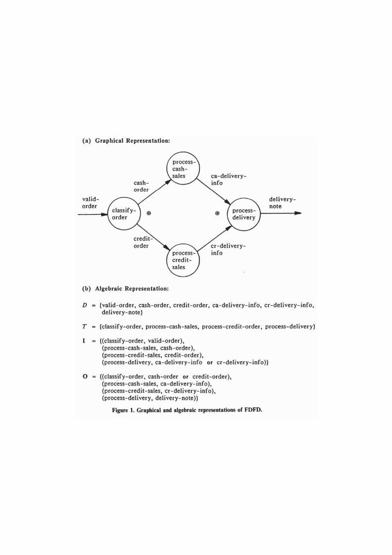
The graphical representation of a sample FDFD and its symbolic equivalent are shown in Figure 1.

To model the behaviour of a system over time, we have also incorporated the notions of token and

firing from Petri nets into FDFD. Tokens can be placed in the data flows of an FDFD. The presence

of a token means that input through a given data flow is ready for a task. A marking of an FDFD is

defined as a set of tokens assigned to its data flows. It indicates the state of a system represented by

the FDFD at a certain point in time. Mathematically, it is a function u: D → N from the set of data

flows D of an FDFD to the set of non-negative integers N. Giv en an FDFD G and a marking u, we

shall call the ordered couple M = (G, u) a marked FDFD.

The marking can be changed by the execution of one or more tasks. A task is said to be executable

if a combination of data flows satisfying its input logic function contains at least one token each, or in

other words, a combination of data satisfying the input logic is available. After the execution of a

task, one token is removed from each of the input data flows, and new tokens are placed in a

combination of data flows satisfying the output logic function. A marking v is said to be reachable

from another marking u if there exists a sequence of executions that changes u into v.

These dynamic elements will provide the basis for analysing the dynamic behaviour of the system.

The analysis will help to detect problems which may not otherwise be apparent in the static model,

such as deadlocks or tasks that will never be activated.

4. CONSISTENCY ANALYSES

To demonstrate the feasibility of the language, a specification system based on FDFD has been

implemented. Details of the specification system can be found in [20] .

One important area in the analysis of a requirements specification is consistency. Consistency

analysis will provide information on the completeness and correctness of a requirements specification.

In addition, if consistency between different decomposition levels in a hierarchical specification is

maintained, it will also reduce the amount of effort required in systems design and maintenance.

Following the line of [5, 4, 16], we shall discuss in this section three types of consistency analyses

useful for requirements specifications. They are global consistency, structural consistency and

behavioural consistency. We shall illustrate how they can be achieved through FDFD.

4.1 Global Consistency Analysis

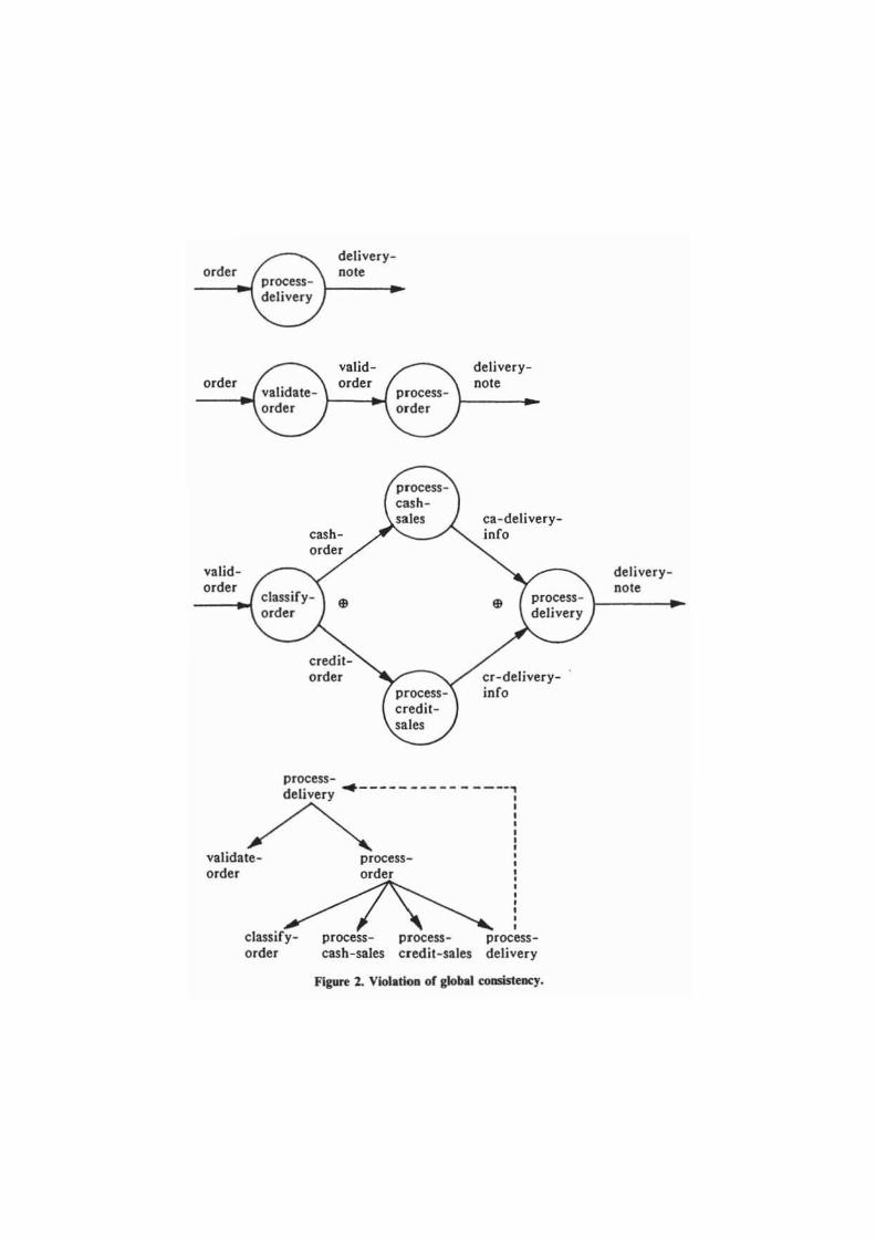
Before we concentrate on the consistency analysis at each abstraction level, we must make sure

that the specification as a whole is defined as a hierarchical structure. Decomposition should not be

done recursively, as illustrated in Figure 2. Otherwise, not only is the resulting specification

confusing to users, but some non-primitive elements may in fact remain undefined. We shall refer to

this type of consistency checking as global consistency analysis.

The decomposition of a task into a hierarchy of subtasks can be regarded as the creation of directed

graphs whose vertices represent data/tasks and whose edges represent parent-child relationships

between data/tasks. A partial ordering would result and the corresponding directed graph should

contain no cycle. The presence of any cycle would imply recursive decomposition. This is illustrated

in the last part of Figure 2.

3

Our algorithm for the detection of cycles is as follows: The directed graph can be represented by

an adjacency matrix A. The entry A(i, j) has a value of 1 if there is an edge from vertex i to vertex j,

and 0 otherwise. From this adjacency matrix, we can compute its corresponding path matrix P, where

the entry P(i, j) has a value of 1 if there is a path from vertex i to vertex j, and 0 otherwise. Hence,

P(i, i) = 1 will indicate the presence of one or more cycles passing through i.

The path matrix P can be computed from the adjacency matrix A by using the Warshall algorithm

[26] :

begin

P := A

for i = 1 to n do

for j = 1 to n do

for k = 1 to n do

P(j, k) := P(j, k) or (P(j, i) and P(i, k))

end.

We can then determine whether or not the hierarchy contains cycles by simply inspecting the diagonal

of P. Any such cycle, if exists, can be located systematically from the original adjacency matrix.

In addition, the precedence analyser developed in [33, 34] can be applied to the adjacency matrix

to generate useful reports for further analyses of the specification.

4.2 Structural Consistency Analysis

In order to spell out the details of a task in a data flow diagram, it can be redrawn as subtasks in

another data flow diagram. One important principle to bear in mind is the balancing rule in structured

analysis [7]: any data flow entering or leaving a parent bubble must be be represented on the lower

level diagram by the same data flow into or out of some child bubble(s). We shall refer to this rule as

structural consistency.

Before we spell out the conditions for structural consistency, we must define the concepts of

external input and output data flows. Given an FDFD G, an external input data flow is defined as a

data flow which is an input to some task in G but not an output to any task in G. The set of all

external input data flows of G will be denoted by ext−input(G). The set ext

−output(G) of external

output data flows is similarly defined.

A necessary and sufficient condition for structural consistency can now be stated. Given a task t0,

let G0

= (D0, {t

0}, I

0, O

0) be the FDFD formed by t

0and its associated input and output flows. Let

G1

= (D1, T

1, I

1, O

1) be the new FDFD formed by decomposing t

0into subtasks. The decomposition

of t0

into subtasks in G1

will be structurally consistent if and only if:

(a) ext−input(G

1) = I

0(t

0), and

(b) ext−output(G

1) = O

0(t

0).

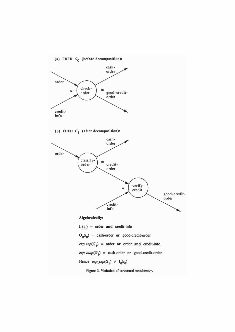
The example in Figure 3 shows a violation of structural consistency.

An algorithm has been developed for finding ext−input(G

1) and ext

−output(G

1). It is summarized

as follows:

(1) Let t1, t

2, ..., t

nbe the tasks of G

1. Relate each t

iwith a data transformation of the form

L(ti) → R(t

i),

where L(ti) = I(t

i) and R(t

i) = O(t

i). Hence represent G

1by a combined transformation

4

L(t1) → R(t

1) and L(t

2) → R(t

2) and ... and L(t

n) → R(t

n).

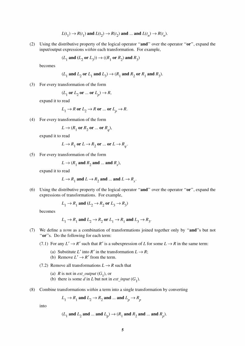
(2) Using the distributive property of the logical operator ‘‘and’’ over the operator ‘‘or’’, expand the

input/output expressions within each transformation. For example,

(L1

and (L2

or L3)) → ((R

1or R

2) and R

3)

becomes

(L1

and L2

or L1

and L3) → (R

1and R

2or R

1and R

3).

(3) For every transformation of the form

(L1

or L2

or ... or Lp) → R,

expand it to read

L1

→ R or L2

→ R or ... or Lp

→ R.

(4) For every transformation of the form

L → (R1

or R2

or ... or Rq),

expand it to read

L → R1

or L → R2

or ... or L → Rq.

(5) For every transformation of the form

L → (R1

and R2

and ... and Rs),

expand it to read

L → R1

and L → R2

and ... and L → Rs.

(6) Using the distributive property of the logical operator ‘‘and’’ over the operator ‘‘or’’, expand the

expressions of transformations. For example,

L1

→ R1

and (L2

→ R2

or L3

→ R3)

becomes

L1

→ R1

and L2

→ R2

or L1

→ R1

and L3

→ R3.

(7) We define a term as a combination of transformations joined together only by ‘‘and’’ s but not

‘‘or’’ s. Do the following for each term:

(7.1) For any L ′ → R ′ such that R ′ is a subexpression of L for some L → R in the same term:

(a) Substitute L ′ into R ′ in the transformation L → R;

(b) Remove L ′ → R ′ from the term.

(7.2) Remove all transformations L → R such that

(a) R is not in ext−output (G

1), or

(b) there is some d in L but not in ext−input (G

1).

(8) Combine transformations within a term into a single transformation by converting

L1

→ R1

and L2

→ R2

and ... and Lp

→ Rp

into

(L1

and L2

and ... and Lp) → (R

1and R

2and ... and R

p).

5

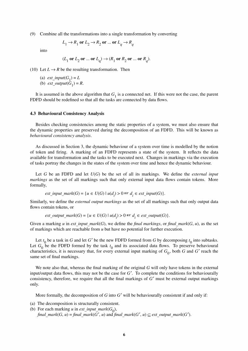
(9) Combine all the transformations into a single transformation by converting

L1

→ R1

or L2

→ R2

or ... or Lq

→ Rq

into

(L1

or L2

or ... or Lq) → (R

1or R

2or ... or R

q).

(10) Let L → R be the resulting transformation. Then

(a) ext−input(G

1) = L

(b) ext−output(G

1) = R.

It is assumed in the above algorithm that G1

is a connected net. If this were not the case, the parent

FDFD should be redefined so that all the tasks are connected by data flows.

4.3 Behavioural Consistency Analysis

Besides checking consistencies among the static properties of a system, we must also ensure that

the dynamic properties are preserved during the decomposition of an FDFD. This will be known as

behavioural consistency analysis.

As discussed in Section 3, the dynamic behaviour of a system over time is modelled by the notion

of token and firing. A marking of an FDFD represents a state of the system. It reflects the data

available for transformation and the tasks to be executed next. Changes in markings via the execution

of tasks portray the changes in the states of the system over time and hence the dynamic behaviour.

Let G be an FDFD and let U(G) be the set of all its markings. We define the external input

markings as the set of all markings such that only external input data flows contain tokens. More

formally,

ext−input

−mark(G) = {u ∈ U(G) | u(d

i) > 0 + d

i∈ ext

−input(G)}.

Similarly, we define the external output markings as the set of all markings such that only output data

flows contain tokens, or

ext−output

−mark(G) = {u ∈ U(G) | u(d

i) > 0 + d

i∈ ext

−output(G)}.

Given a marking u in ext−input

−mark(G), we define the final markings, or final

−mark(G, u), as the set

of markings which are reachable from u but hav e no potential for further execution.

Let t0

be a task in G and let G ′ be the new FDFD formed from G by decomposing t0

into subtasks.

Let G0

be the FDFD formed by the task t0

and its associated data flows. To preserve behavioural

characteristics, it is necessary that, for every external input marking of G0, both G and G ′ reach the

same set of final markings.

We note also that, whereas the final marking of the original G will only have tokens in the external

input/output data flows, this may not be the case for G ′. To complete the conditions for behaviourally

consistency, therefore, we require that all the final markings of G ′ must be external output markings

only.

More formally, the decomposition of G into G ′ will be behaviourally consistent if and only if:

(a) The decomposition is structurally consistent.

(b) For each marking u in ext−input

−mark(G

0),

final−mark(G, u) = final

−mark(G ′, u) and final

−mark(G ′, u) ⊆ ext

−output

−mark(G ′).

6

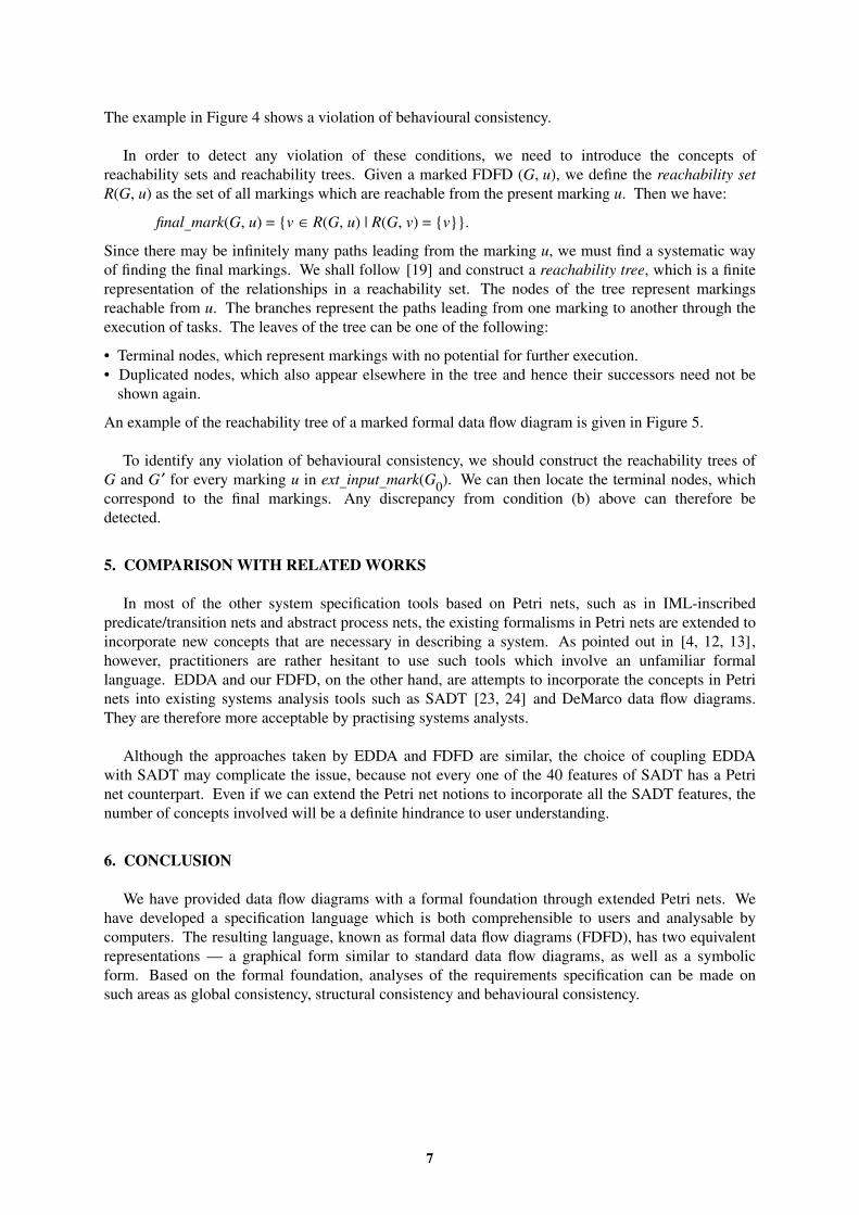
The example in Figure 4 shows a violation of behavioural consistency.

In order to detect any violation of these conditions, we need to introduce the concepts of

reachability sets and reachability trees. Given a marked FDFD (G, u), we define the reachability set

R(G, u) as the set of all markings which are reachable from the present marking u. Then we have:

final−mark(G, u) = {v ∈ R(G, u) | R(G, v) = {v}}.

Since there may be infinitely many paths leading from the marking u, we must find a systematic way

of finding the final markings. We shall follow [19] and construct a reachability tree, which is a finite

representation of the relationships in a reachability set. The nodes of the tree represent markings

reachable from u. The branches represent the paths leading from one marking to another through the

execution of tasks. The leaves of the tree can be one of the following:

• Terminal nodes, which represent markings with no potential for further execution.

• Duplicated nodes, which also appear elsewhere in the tree and hence their successors need not be

shown again.

An example of the reachability tree of a marked formal data flow diagram is given in Figure 5.

To identify any violation of behavioural consistency, we should construct the reachability trees of

G and G ′ for every marking u in ext−input

−mark(G

0). We can then locate the terminal nodes, which

correspond to the final markings. Any discrepancy from condition (b) above can therefore be

detected.

5. COMPARISON WITH RELATED WORKS

In most of the other system specification tools based on Petri nets, such as in IML-inscribed

predicate/transition nets and abstract process nets, the existing formalisms in Petri nets are extended to

incorporate new concepts that are necessary in describing a system. As pointed out in [4, 12, 13],

however, practitioners are rather hesitant to use such tools which involve an unfamiliar formal

language. EDDA and our FDFD, on the other hand, are attempts to incorporate the concepts in Petri

nets into existing systems analysis tools such as SADT [23, 24] and DeMarco data flow diagrams.

They are therefore more acceptable by practising systems analysts.

Although the approaches taken by EDDA and FDFD are similar, the choice of coupling EDDA

with SADT may complicate the issue, because not every one of the 40 features of SADT has a Petri

net counterpart. Even if we can extend the Petri net notions to incorporate all the SADT features, the

number of concepts involved will be a definite hindrance to user understanding.

6. CONCLUSION

We hav e provided data flow diagrams with a formal foundation through extended Petri nets. We

have dev eloped a specification language which is both comprehensible to users and analysable by

computers. The resulting language, known as formal data flow diagrams (FDFD), has two equivalent

representations — a graphical form similar to standard data flow diagrams, as well as a symbolic

form. Based on the formal foundation, analyses of the requirements specification can be made on

such areas as global consistency, structural consistency and behavioural consistency.

7

ACKNOWLEDGEMENTS

This research is supported in part by a Hong Kong & China Gas research grant and a University of

Hong Kong research grant. The authors are indebted to Ronald Stamper of the London School of

Economics, University of London, and S.W. Ho and C.F. Chong of the University of Hong Kong for

their invaluable comments and suggestions.

REFERENCES

[1] T. Agerwala, ‘‘Putting Petri nets to work’’, IEEE Computer 12 (12): 85−94 (1979).

[2] L.L. Beck and T.E. Perkins, ‘‘A survey of software engineering practice: tools, methods, and

results’’, IEEE Transactions on Software Engineering SE-9 (5): 541−561 (1983).

[3] M.A. Colter, ‘‘Evolution of the structured methodologies’’, in Advanced System Development /

Feasibility Techniques, J.D. Couger, M.A. Colter, and R.W. Knapp (eds.), Wiley, New York, NY,

pp. 73−96 (1982).

[4] A.M. Davis, ‘‘The design of a family of application-oriented requirements languages’’, IEEE

Computer 15 (5): 21−28 (1982).

[5] A.M. Davis and T.G. Rauscher, ‘‘Formal techniques and automatic processing to ensure

correctness in requirements specifications’’, in Proceedings of the IEEE Conference on

Specifications of Reliable Software, M.V. Zelkowitz (ed.), IEEE Computer Society Press, New

York, NY, pp. 15−35 (1979).

[6] N.M. Delisle, D.E. Menicosy, and N.L. Kerth, ‘‘Tools for supporting structured analysis’’, in

Automated Tools for Information Systems Design, H.-J. Schneider and A.I. Wasserman (eds.),

Elsevier, Amsterdam, The Netherlands, pp. 11−20 (1982).

[7] T. DeMarco, Structured Analysis and System Specification, Yourdon Press Computing Series,

Prentice Hall, Englewood Cliffs, NJ (1979).

[8] C.P. Gane and T. Sarson, Structured Systems Analysis: Tools and Techniques, Prentice Hall,

Englewood Cliffs, NJ (1979).

[9] M.A. Jackson, Principles of Program Design, Academic Press, London, UK (1975).

[10] M.A. Jackson, System Development, Prentice Hall International Series in Computer Science,

Prentice Hall, London, UK (1983).

[11] G.R. Kampen, ‘‘SWIFT: a requirements specification system for software’’, in Requirements

Engineering Environments: Proceedings of the International Symposium on Current Issues of

Requirements Engineering Environments, Y. Ohno (ed.), Elsevier, Amsterdam, The Netherlands,

pp. 77−84 (1982).

[12] J. Martin, Program Design which is Pro vably Correct, Savant Institute, Carnforth, Lancashire,

UK (1983).

[13] J. Martin, An Information Systems Manifesto, Prentice Hall, Englewood Cliffs, NJ (1984).

[14] L.J. Mekly, A Systems Approach to Software Design Representation, PhD Thesis, Northwestern

University, Evanston, IL (1979).

[15] L.J. Mekly and S.S. Yau, ‘‘Software design representation using abstract process networks’’,

IEEE Transactions on Software Engineering SE-6 (5): 420−435 (1980).

[16] T.J. Miller and B.J. Taylor, ‘‘A system requirements methodology’’, in Proceedings of

ELECTRO 1981, IEEE Computer Society Press, New York, NY, pp. 18.5.1−18.5.5 (1981).

8

[17] K.T. Orr, Structured Systems Development, Yourdon Press Computing Series, Prentice Hall,

Englewood Cliffs, NJ (1977).

[18] J.L. Peterson, ‘‘Petri nets’’, ACM Computing Surveys 9 (3): 223−252 (1977).

[19] J.L. Peterson, Petri Net Theory and the Modeling of Systems, Prentice Hall, Englewood Cliffs,

NJ (1981).

[20] L. Pong, Formal Data Flow Diagrams (FDFD): a Petri-Net Based Requirements Specification

Language, MPhil Thesis, The University of Hong Kong, Pokfulam, Hong Kong (1986).

[21] W. Reisig, Petri Nets: an Introduction, EATCS Monographs on Theoretical Computer Science,

vol. 4, Springer, Berlin, Germany (1985).

[22] G. Richter and R. Durchholz, ‘‘IML-inscribed high-level Petri nets’’, in Information Systems

Design Methodologies, a Comparative Review: Proceedings of the IFIP WG 8.1 Working

Conference (CRIS 1982), T.W. Olle, H.G. Sol, and A.A. Verrijn-Stuart (eds.), Elsevier,

Amsterdam, The Netherlands, pp. 335−368 (1982).

[23] D.T. Ross, ‘‘Structured analysis (SA): a language for communicating ideas’’, in Advanced

System Development / Feasibility Techniques, J.D. Couger, M.A. Colter, and R.W. Knapp (eds.),

Wiley, New York, NY, pp. 135−163 (1982).

[24] D.T. Ross and K.E. Schoman, ‘‘Structured analysis for requirements definition’’, in Classics in

Software Engineering, E. Yourdon (ed.), Yourdon Press Computing Series, Prentice Hall,

Englewood Cliffs, NJ, pp. 365−385 (1979).

[25] W. Trattnig and H. Kerner, ‘‘EDDA: a very-high-level programming and specification language

in the style of SADT’’, in Proceedings of the 4th Annual International Computer Software and

Applications Conference (COMPSAC 1980), IEEE Computer Society Press, New York, NY, pp.

436−443 (1980).

[26] J.P. Tremblay and P.G. Sorenson, An Introduction to Data Structures with Applications,

McGraw-Hill, New York, NY (1976).

[27] T.H. Tse, ‘‘A unified algebraic view of structured systems development models’’, Doctoral

Consortium, 6th International Conference on Information Systems, Indianapolis, IN (1985).

[28] T.H. Tse, ‘‘An algebraic formulation for structured systems development tools’’, Hong Kong

Computer Journal 2 (4): 44−49 (1986).

[29] T.H. Tse, ‘‘Integrating the structured analysis and design models: an initial algebra approach’’,

Australian Computer Journal 18 (3): 121−127 (1986).

[30] T.H. Tse, ‘‘Tow ards a unified algebraic view of structured systems development models’’, ACM

SIGMIS Database 17 (4) (1986).

[31] T.H. Tse, ‘‘Integrating the structured analysis and design models: a category-theoretic

approach’’, Australian Computer Journal 19 (1): 25−31 (1987).

[32] T.H. Tse and L. Pong, ‘‘An examination of requirements specification languages’’, The

Computer Journal 34 (2): 143−152 (1991).

[33] S.J. Waters, ‘‘CAM 01: a precedence analyser’’, The Computer Journal 19 (2): 122−126 (1976).

[34] S.J. Waters, ‘‘CAM 02: a structured precedence analyser’’, The Computer Journal 20 (1): 2−5

(1977).

[35] V. Weinberg, Structured Analysis, Yourdon Press Computing Series, Prentice Hall, Englewood

Cliffs, NJ (1980).

9

[36] E. Yourdon and L.L. Constantine, Structured Design: Fundamentals of a Discipline of Computer

Program and Systems Design, Yourdon Press Computing Series, Prentice Hall, Englewood

Cliffs, NJ (1979).

APPENDIX

A Brief Summary of Petri Nets

A Petri net is a directed bipartite graph consisting of two types of nodes — places and transitions.

Algebraically, it is defined as a 4-tuple C = (P, T, I, O) such that:

• P = {p1, p

2, ..., p

n}, where n ≥ 1, is a finite set of places.

• T = {t1, t

2, ..., t

m}, where m ≥ 1, is a finite set of transitions.

• P and T are disjoint.

• I: T → 2P and O: T → 2P, where 2P denote the power set of P, are functions which map transitions

to sets of places. I is called the input function and O the output function.

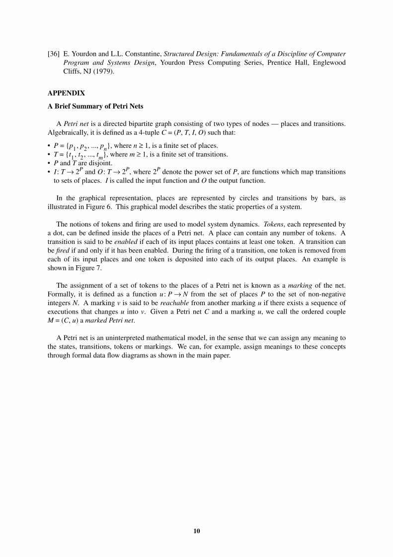
In the graphical representation, places are represented by circles and transitions by bars, as

illustrated in Figure 6. This graphical model describes the static properties of a system.

The notions of tokens and firing are used to model system dynamics. Tokens, each represented by

a dot, can be defined inside the places of a Petri net. A place can contain any number of tokens. A

transition is said to be enabled if each of its input places contains at least one token. A transition can

be fired if and only if it has been enabled. During the firing of a transition, one token is removed from

each of its input places and one token is deposited into each of its output places. An example is

shown in Figure 7.

The assignment of a set of tokens to the places of a Petri net is known as a marking of the net.

Formally, it is defined as a function u: P → N from the set of places P to the set of non-negative

integers N. A marking v is said to be reachable from another marking u if there exists a sequence of

executions that changes u into v. Giv en a Petri net C and a marking u, we call the ordered couple

M = (C, u) a marked Petri net.

A Petri net is an uninterpreted mathematical model, in the sense that we can assign any meaning to

the states, transitions, tokens or markings. We can, for example, assign meanings to these concepts

through formal data flow diagrams as shown in the main paper.

10

(a) Graphical Representation:

valid­order

cash­ordcr

classify­order

credit­order

(IJ) AllelJrale Representation:

process­cash-

ca-delivery­info

process­delivery

cr-delivery­info

delivery­note

D _ {valid-order, cash-order, credit-order, ca-delivery-info. cr-delivery-info, delivery- note}

T - {classify-order. process-cash-sales, process-credit-order, process-delivery}

I .. «classify-order, valid-order), (process-cash-sales, cash-order), (process-c red it -sales, cred it -order), (process-delivery, ca-delivery - info or cr-delivery-info»

o - ((classify-order, cash-order or credit-order), (process- cash-sales, ca- delivery- info), (process-credit-sales, cr-delivery- info), (process-delivery. delivery- note)}

Figure 1. Graphical and algebrak representations of FOFO.

order delivery­note __ ---<., process­

delivery

valid-order order ___ .j validate- '--.... 01

valid -order

order I

cash-order

.. credit­order

process­order

delivery­note

ca-delivery-inro

.. cr-delivery­inro

process-. 4----- --- -- - ----.,

A i validate- process- : order order :

cJassiry­order

process­cash-sales

process­credit-sales

, , , , , , process­delivery

Figwe 2. VioI.lion or Ck)bal roDSisteacy.

delivery-note

(a) FDFD GO (before decomposltion):

order

cred it ­info

• check­order

..

cash­order

good-credit-order

(b) FDFD G1 (aHer decomposition):

order

classify­order

..

Algebraically:

cash­order

credit-order

credit­info

[oUr} = order and credit-info

0o(tr} = cash-order or good-credit-order

exp_inp(G1) = order or order and credit-info

exp_outp(Gt ) = cash-order or good-credit-order

Hence up _inp{G1) *- [o(tr}

Figure 3. Violation or structural coMistency.

good-credit­order

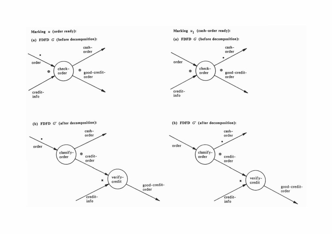
Markin. tI (order rudy):

(a) FOFO G (bdore decomposition):

credit­info

cash­order

.. . good-credlt-order

(b) FOFO G' (after decomposition):

• order~ /"

classify- ) .. order

cash-ordey

credit-order

-credit­info

good-credil­order

Markin. til (ush-order rudy):

(a) FOFO G (bdore decomposition):

order

credit­info

check­order

•

..

cash­order

Bood-credit-order

(b) FOFO G' (afler decomposition):

~ order

cash-order

•

order credit-~''''U'J: order

-credit­info

verify­credit

good -credil ­order

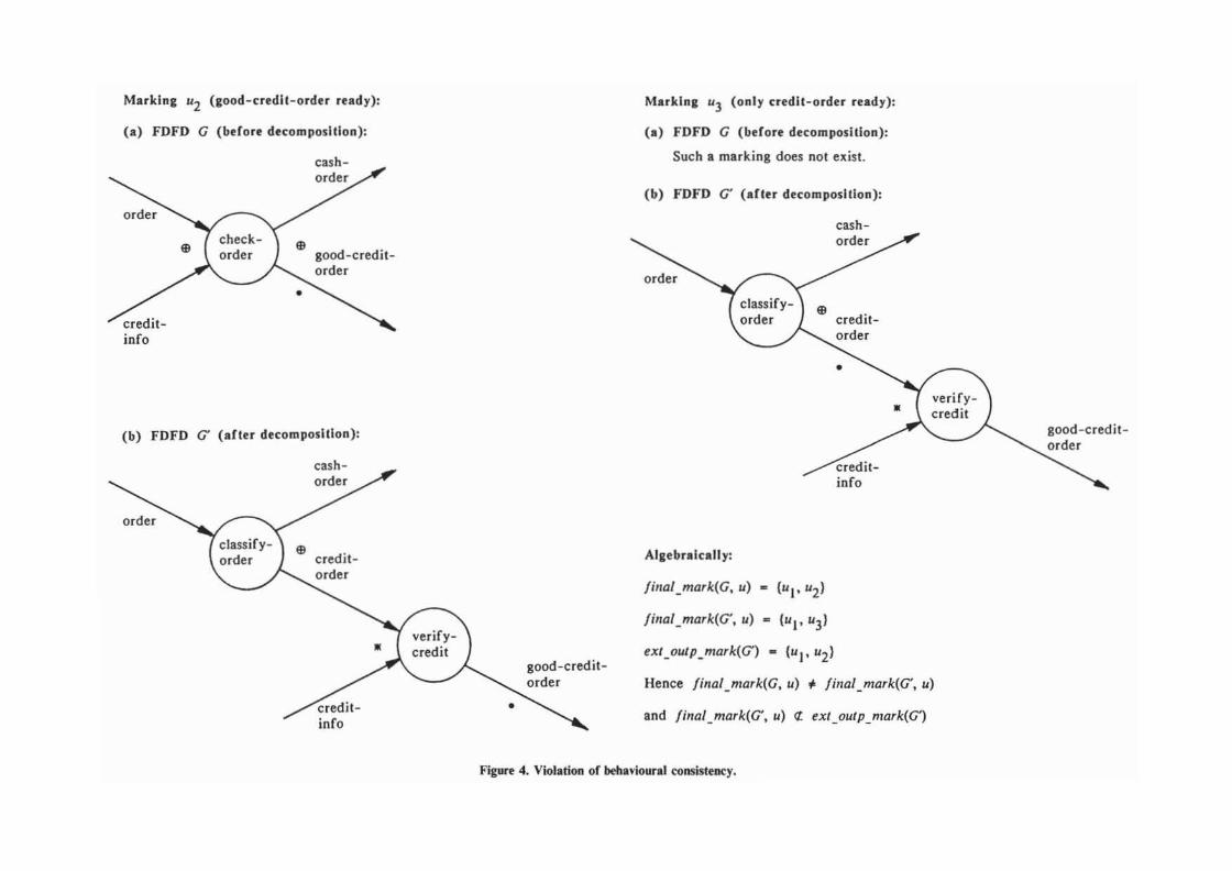
Marklnl u2 (Kood-c:redlt-ordu rudy):

(a) FDFD G (bdore dec:omposltlon):

order

credit­info

cash­order

" od . go -credlt-order

•

(b) FDFD G' (aUer decomposillon):

" . credlt-order

credit ­info

verify­credit

•

good-credit­order

Marklne u3 (only credit-order rudy):

(a) FDFD G (bdore decomposition):

Such a marking does not exist.

(b) FDFD G' (aUer decomposition):

order

cash­order

classify­order " . cred ll-

A1eebralully:

jillaf_mark(G, u) .. (ul' u2)

jillal_mark(G', u) - (u l , u3)

~XI_oulp_mark(G') .. (up u2)

order

•

credit­info

Hence jina'-mark(G, u) ~ jillal_mark(G', u)

and jillal_mark(G', u) ([. ~xt_outp_mark(G')

Figure 4. Vtolation of behavioural consistency.

good-credil ­order

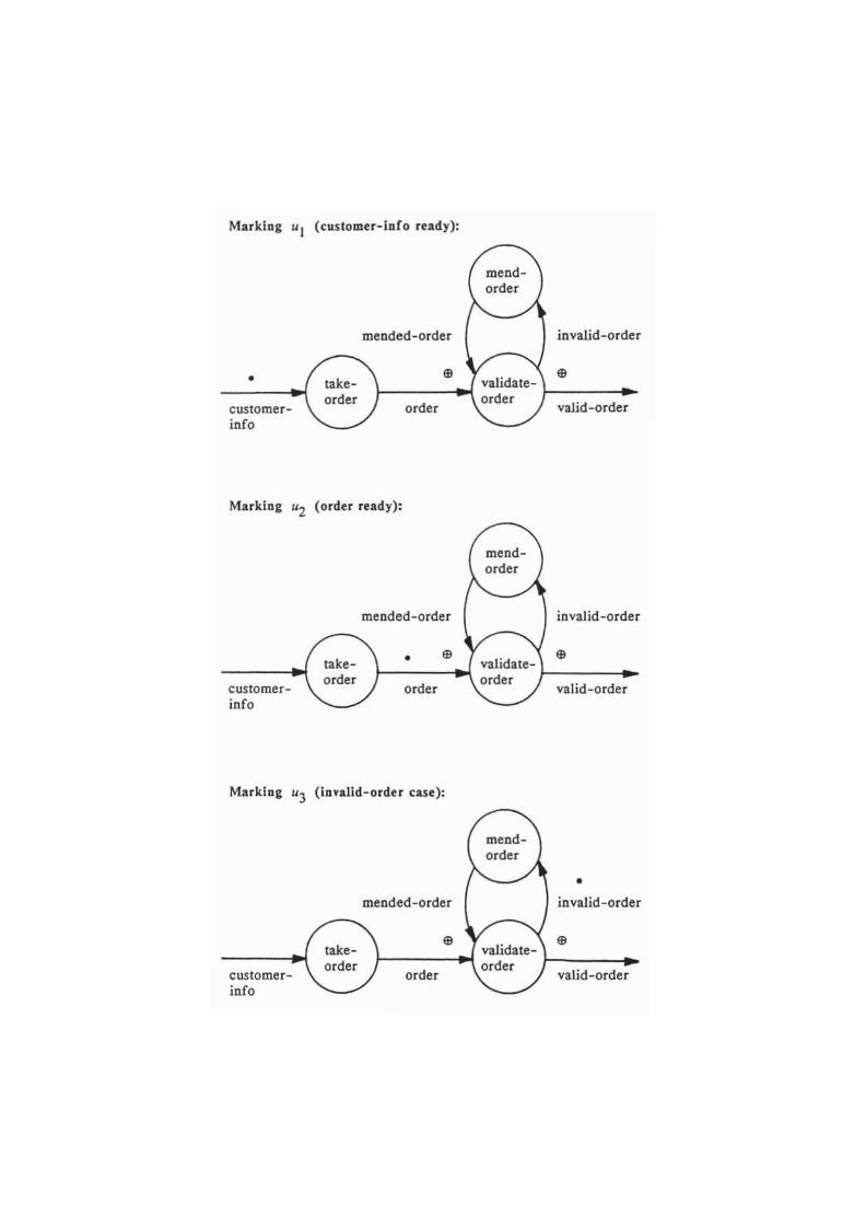
Marking ul ( customer- Iofo ready):

•

customer­info

take­order

meoded-order

meod­order

iovalid-orde r

" " I----~_I validate- '-_ _ _ _

order order r

valid-orde r

Markio g u2 (order ready):

custome r­info

take­order

mended-orde r

mend­order

invalid-orde r

. " " '-___ .., validate- '-------iO~ ,--- order r

order valid-order

Marking uJ (inn lid- orde r case):

meod-order '" ./ •

mended-order invalid-order

/ '\ " /~'<

" take- validate-order

order order

valid-order customer- "- ./ "- / info

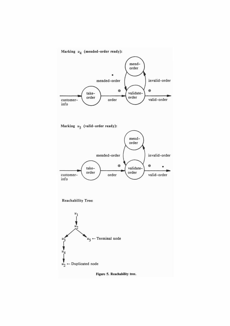
Markiol 1.14 (mended-order ready):

• mended-order invalid-order

" .. validate- )-____ _

I-----;~ order order custorner­

info

Markiol Us (valid-order ready):

mended-order

'\ take- " order

order customer- \... ./ info

Reachability Tree:

"I

~ ",

~"5 - T"min.I node

",

~ - Doplie.ted node

/ '\ mend­order "'_/

>I" '\ validate-order

./

Figun 5. Readl.bility tree.

valid-order

invalid-order

" • valid-order