Embed Size (px)
Citation preview

To the University of Wyoming:The members of the Committee approve the thesis of Troy E. Lake, Jr. presented on
28 April 2017.
Dr. Dimitri Mavriplis, Chairperson
Dr. Craig Douglas, External Department Member
Dr. Michael Stoellinger
Dr. Brian Allan
APPROVED:
Dr. Carl P. Frick, Head, Department of Mechanical Engineering
Dr. Michael Pishko, Dean, College of Engineering and Applied Science
Lake, Jr., Troy E., Adjoint based, Error Controlled, Loosely Coupled, Unstructured Design
Optimization and Adaptive Mesh Refinement Using FUN3D, M.S., De-
partment of Mechanical Engineering, May, 2017.
Adjoint-based design problems are dependent on the sensitivities from the CFD solu-
tion. Current best practices for these adjoint based design problems use fixed-complexity
computational meshes that are built using developed best practices. An issue with these
fixed-complexity computational meshes is that flow features may not be properly or com-
pletely captured. To improve the accuracy of the solution and the sensitivities, the mesh
can be adaptively refined to reduce the discretization error within the flow solution. By
adapting the mesh, the size of the mesh may be reduced as well, increasing the computa-
tional efficiency of the design problem. The computational efficiency of the design problem
may also be improved with the use of progressive design variable parameterization. This re-
search focuses on developing methodologies for variations of current best practices methods
for design optimization problems including the use of adaptive mesh refinement. The design
optimization and mesh adaption processes utilize the built-in tools within FUN3D, linked to
the SNOPT optimizer for geometry optimization. To justify the benefits of the coupled mesh
adaptation and design optimization, the final value of the objective function, complexity of
the computational mesh, and the Optimization Complexity Function for each case are used
as comparison points. An inviscid, non-lifting airfoil, and a viscous, lifting airfoil are used
as test cases for this research. The baseline case uses a fixed parameterization scheme, and
comparison cases exploit progressive parameterization to aid in creating optimal shapes while
avoiding the introduction of irregular shape features. Fixed complexity mesh optimization
cases are compared with loosely coupled adaptive mesh refinement (AMR) and optimization
cases. The family of fixed-complexity meshes are also used in a progressive mesh complexity
method, starting with the coarse mesh and then transitioning the final design to the next
finest mesh. During the research, it was found that the more design variables used during the
optimization, the better the resulting optimal airfoil. For a 31 design-variable case, the final
1
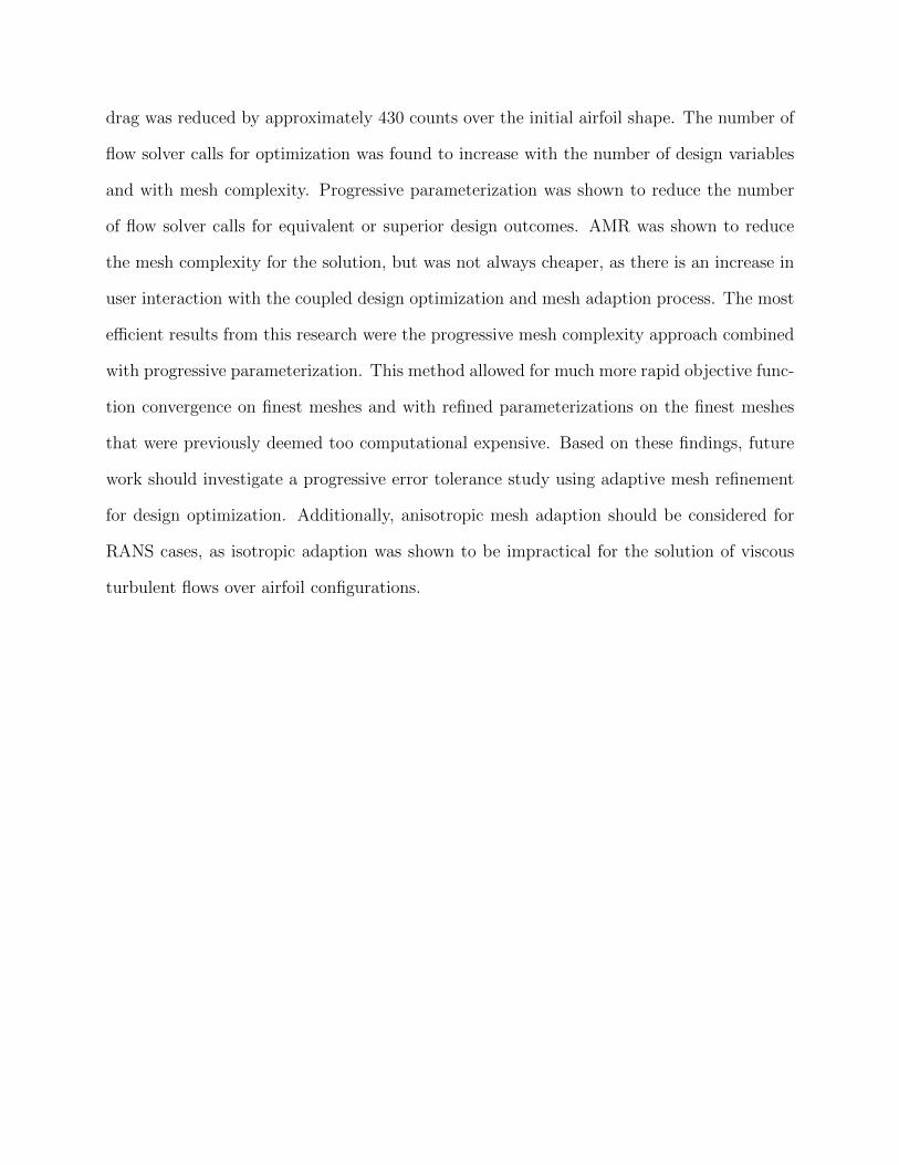
drag was reduced by approximately 430 counts over the initial airfoil shape. The number of
flow solver calls for optimization was found to increase with the number of design variables
and with mesh complexity. Progressive parameterization was shown to reduce the number
of flow solver calls for equivalent or superior design outcomes. AMR was shown to reduce
the mesh complexity for the solution, but was not always cheaper, as there is an increase in
user interaction with the coupled design optimization and mesh adaption process. The most
efficient results from this research were the progressive mesh complexity approach combined
with progressive parameterization. This method allowed for much more rapid objective func-
tion convergence on finest meshes and with refined parameterizations on the finest meshes
that were previously deemed too computational expensive. Based on these findings, future
work should investigate a progressive error tolerance study using adaptive mesh refinement
for design optimization. Additionally, anisotropic mesh adaption should be considered for
RANS cases, as isotropic adaption was shown to be impractical for the solution of viscous
turbulent flows over airfoil configurations.

ADJOINT BASED, ERROR CONTROLLED,
LOOSELY COUPLED, UNSTRUCTURED DESIGN
OPTIMIZATION AND ADAPTIVE MESH
REFINEMENT USING FUN3D
by
Troy E. Lake, Jr., B. S. A. E.
A thesis submitted to theDepartment of Mechanical Engineering
and theUniversity of Wyoming
in partial fulfillment of the requirementsfor the degree of
MASTER OF SCIENCEin
MECAHNICAL ENGINEERING
Laramie, WyomingMay 2017

Copyright © 2017
by
Troy E. Lake, Jr.
ii

To my family, both related and the friends that have become family. Without you, this
would not have been possible.
iii

Contents
List of Figures viii
List of Tables xi
Acknowledgments xiii
Chapter 1 Introduction 1
1.1 Motivation . . . . . . . . . . . . . . . . . . . . . . . . . . . . . . . . . . . . . 1
1.2 Literature Survey . . . . . . . . . . . . . . . . . . . . . . . . . . . . . . . . . 4
1.2.1 Design Optimization . . . . . . . . . . . . . . . . . . . . . . . . . . . 4
1.2.2 Shape Parameterization Methods . . . . . . . . . . . . . . . . . . . . 5
1.2.3 Adaptive Mesh Refinement . . . . . . . . . . . . . . . . . . . . . . . . 7
1.2.4 Design Optimization Coupled with Adaptive Mesh Refinement . . . . 7
Chapter 2 Methodology 9
2.1 Computational Mesh Generation . . . . . . . . . . . . . . . . . . . . . . . . 9
2.1.1 Collared Computational Mesh Design . . . . . . . . . . . . . . . . . . 10
2.1.2 Family of Computational Meshes . . . . . . . . . . . . . . . . . . . . 11
2.1.3 Adaptive Mesh Refinement . . . . . . . . . . . . . . . . . . . . . . . . 12
2.1.4 Complexity of Computational Mesh . . . . . . . . . . . . . . . . . . . 13
2.2 Design Optimization . . . . . . . . . . . . . . . . . . . . . . . . . . . . . . . 14
iv

2.2.1 General Approach . . . . . . . . . . . . . . . . . . . . . . . . . . . . . 14
2.2.2 Fixed Design Variable Parameterization . . . . . . . . . . . . . . . . 17
2.2.3 Progressive Design Variable Parameterization . . . . . . . . . . . . . 17
2.2.4 Grid Complexities . . . . . . . . . . . . . . . . . . . . . . . . . . . . 18
2.2.5 Loosely coupled adaptive mesh refinement and design optimization . 18
2.2.6 Setting and Managing Design Variable Bounds . . . . . . . . . . . . . 19
2.3 Overall Strategies . . . . . . . . . . . . . . . . . . . . . . . . . . . . . . . . . 20
Chapter 3 Numerical Approach 22
3.1 FUN3D . . . . . . . . . . . . . . . . . . . . . . . . . . . . . . . . . . . . . . 22
3.1.1 Flow Solver . . . . . . . . . . . . . . . . . . . . . . . . . . . . . . . . 23
3.1.2 Adjoint-Based Design Optimizer . . . . . . . . . . . . . . . . . . . . . 23
3.2 Mesh Generation . . . . . . . . . . . . . . . . . . . . . . . . . . . . . . . . . 24
3.3 Data Reduction . . . . . . . . . . . . . . . . . . . . . . . . . . . . . . . . . . 24
3.4 Computational Power . . . . . . . . . . . . . . . . . . . . . . . . . . . . . . . 25
Chapter 4 Results for Test Case 1: Transonic, Inviscid, Non-lifting, Drag
Minimization 26
4.1 Problem Description . . . . . . . . . . . . . . . . . . . . . . . . . . . . . . . 27
4.2 Solver Setup . . . . . . . . . . . . . . . . . . . . . . . . . . . . . . . . . . . . 27
4.3 Fixed-Complexity Computational Mesh Generation . . . . . . . . . . . . . . 29
4.4 Fixed-Complexity Computational Mesh, Fixed Parameterization Results . . 32
4.4.1 Three design-variable . . . . . . . . . . . . . . . . . . . . . . . . . . . 32
4.4.2 Seven Design Variables . . . . . . . . . . . . . . . . . . . . . . . . . . 37
4.4.3 Fifteen Design Variables . . . . . . . . . . . . . . . . . . . . . . . . . 37
4.4.4 Thirty-One Design Variables . . . . . . . . . . . . . . . . . . . . . . . 39
v

4.4.5 Fixed-Complexity Computational Mesh, Fixed Parameterization, Max
Bounds . . . . . . . . . . . . . . . . . . . . . . . . . . . . . . . . . . 41
4.5 Fixed-Complexity Computational Mesh, Progressive Parameterization . . . . 42
4.5.1 Fixed Bounds . . . . . . . . . . . . . . . . . . . . . . . . . . . . . . . 42
4.5.2 Max Bounds . . . . . . . . . . . . . . . . . . . . . . . . . . . . . . . . 44
4.6 Adapted Mesh, Fixed Parameterization Results . . . . . . . . . . . . . . . . 45
4.7 Adapted Mesh, Progressive Parameterization Results . . . . . . . . . . . . . 47
4.8 Adapted Mesh: Design followed by AMR . . . . . . . . . . . . . . . . . . . . 49
4.9 Progressive, Fixed-Computational Mesh Refinement . . . . . . . . . . . . . . 50
4.9.1 Fixed Design Variable Parameterization . . . . . . . . . . . . . . . . 50
4.9.2 Progressive Design Variable Parameterization . . . . . . . . . . . . . 52
Chapter 5 Results for Test Case 2: Transonic, RANS, Lift Penalized, Drag
Minimization 54
5.1 Problem Description . . . . . . . . . . . . . . . . . . . . . . . . . . . . . . . 54
5.2 Solver Setup . . . . . . . . . . . . . . . . . . . . . . . . . . . . . . . . . . . . 55
5.3 Fixed-Complexity Computational Mesh Generation . . . . . . . . . . . . . . 56
5.4 Fixed-Complexity Computational Mesh, Fixed Parameterization Results . . 57
5.5 Fixed-Complexity Computational Mesh, Fixed Parameterization Results . . 60
5.5.1 Seven Design-Variables . . . . . . . . . . . . . . . . . . . . . . . . . . 60
5.6 Fixed-Complexity Computational Mesh, Progressive Parameterization Results 61
5.7 Adaptive Mesh Refinement . . . . . . . . . . . . . . . . . . . . . . . . . . . . 62
Chapter 6 Conclusions and Lessons Learned 63
6.1 Conclusions for Test Case 1 . . . . . . . . . . . . . . . . . . . . . . . . . . . 63
6.2 Conclusions for Test Case 2 . . . . . . . . . . . . . . . . . . . . . . . . . . . 64
6.3 General Conclusions . . . . . . . . . . . . . . . . . . . . . . . . . . . . . . . 64
vi

6.4 Operational Lessons Learned . . . . . . . . . . . . . . . . . . . . . . . . . . . 65
6.4.1 Fully converging the flow solution and adjoint solution . . . . . . . . 65
6.4.2 Fully converging mesh movement problem . . . . . . . . . . . . . . . 66
6.4.3 Tightening bounds . . . . . . . . . . . . . . . . . . . . . . . . . . . . 66
6.4.4 Isotropic Mesh Adaption . . . . . . . . . . . . . . . . . . . . . . . . . 67
6.4.5 Restart vs Uniform start for design problems . . . . . . . . . . . . . . 68
6.4.6 Bound Limits on Adapted Meshes . . . . . . . . . . . . . . . . . . . . 69
6.5 Recommendations for Future Work . . . . . . . . . . . . . . . . . . . . . . . 69
Appendix A Numerical Approach Figures 71
Bibliography 74
vii

List of Figures
2.1 Family of fixed-complexity computational meshes . . . . . . . . . . . . . . . 10
2.2 Sample collared mesh . . . . . . . . . . . . . . . . . . . . . . . . . . . . . . . 11
2.3 Airfoil . . . . . . . . . . . . . . . . . . . . . . . . . . . . . . . . . . . . . . . 13
2.4 Design parameterization locations . . . . . . . . . . . . . . . . . . . . . . . . 16
2.5 Bound size comparison as it applies to reparameterization . . . . . . . . . . 20
4.1 Sample half mesh . . . . . . . . . . . . . . . . . . . . . . . . . . . . . . . . . 27
4.2 Overall view of fixed-complexity computational meshes . . . . . . . . . . . . 29
4.3 Zoomed view of fixed-complexity computational meshes . . . . . . . . . . . . 30
4.4 Near-field view of fixed-complexity computational meshes . . . . . . . . . . . 30
4.5 Airfoil view of fixed-complexity computational meshes . . . . . . . . . . . . . 31
4.6 Drag convergence for the fixed-complexity computational mesh on the initial
shape of a NACA-0012m . . . . . . . . . . . . . . . . . . . . . . . . . . . . . 31
4.7 Mach convergence for the family of fixed-complexity computational meshes . 32
4.8 Surface coefficient of pressure profiles for the family of meshes . . . . . . . . 32
4.9 Shock location view of surface coefficient of pressure . . . . . . . . . . . . . . 33
4.10 Optimality, and objective function convergence from SNOPT for the family
of fixed-complexity computational meshes with 3 design-variable for the first
optimization circuit . . . . . . . . . . . . . . . . . . . . . . . . . . . . . . . . 33
viii

4.11 Flow solver call convergence for the family of fixed-complexity computational
meshes with 3 design-variable for the first optimization circuit . . . . . . . . 34
4.12 Family of fixed-complexity computational meshes density (rho) residual con-
vergence (red line) and drag values flow solution (black line) convergence
history for 3 design-variable first optimization circuit . . . . . . . . . . . . . 34
4.13 Family of fixed-complexity computational meshes density (rho) adjoint resid-
ual convergence . . . . . . . . . . . . . . . . . . . . . . . . . . . . . . . . . . 35
4.14 Mach contours with 3 design-variable for the first optimization circuit . . . . 35
4.15 Mach convergence for successive optimization circuits . . . . . . . . . . . . . 38
4.16 Mach convergence for successive optimization circuits . . . . . . . . . . . . . 39
4.17 Various views of the discretization-error adapted computational meshes . . . 46
4.18 Mach contour comparison of adapted and fixed-complexity computational
meshes . . . . . . . . . . . . . . . . . . . . . . . . . . . . . . . . . . . . . . . 46
4.19 Example of adaptive mesh refinement mesh size growth . . . . . . . . . . . . 48
5.1 Overall view of fixed-complexity computational meshes . . . . . . . . . . . . 57
5.2 Zoomed view of fixed-complexity computational meshes . . . . . . . . . . . . 57
5.3 Near-field view of fixed-complexity computational meshes . . . . . . . . . . . 58
5.4 Airfoil view of fixed-complexity computational meshes . . . . . . . . . . . . . 58
5.5 Lift and drag convergence for the fixed-complexity computational mesh on
the initial shape of the TMA-0712 . . . . . . . . . . . . . . . . . . . . . . . . 59
5.6 Mach convergence for the family of fixed-complexity computational meshes . 59
5.7 Surface coefficient of pressure profiles for the family of meshes . . . . . . . . 60
5.8 Example of design result from under-resolved computational mesh . . . . . . 60
5.9 Initial and final Cp profiles for 7 and 15 design variables . . . . . . . . . . . . 62
6.1 Unconverged residuals . . . . . . . . . . . . . . . . . . . . . . . . . . . . . . 66
ix

6.2 Bound limit comparison . . . . . . . . . . . . . . . . . . . . . . . . . . . . . 67
A.1 Computational mesh adaption process within FUN3D . . . . . . . . . . . . . 72
A.2 Design optimization process within FUN3D . . . . . . . . . . . . . . . . . . 72
A.3 Optimization then adaptation . . . . . . . . . . . . . . . . . . . . . . . . . . 73
A.4 Adaption then optimization . . . . . . . . . . . . . . . . . . . . . . . . . . . 73
x

List of Tables
2.1 Node count for collared and non-collared meshes at various boundary far field
distances . . . . . . . . . . . . . . . . . . . . . . . . . . . . . . . . . . . . . . 11
2.2 Collar spacing (unit lengths) . . . . . . . . . . . . . . . . . . . . . . . . . . . 11
3.1 Computational resources used for research . . . . . . . . . . . . . . . . . . . 25
4.1 Pointwise settings for test case 1 . . . . . . . . . . . . . . . . . . . . . . . . . 29
4.2 3 design-variable first optimization circuit tabulated values . . . . . . . . . . 36
4.3 3 design-variable final design tabulated values . . . . . . . . . . . . . . . . . 37
4.4 7 design-variable final design tabulated values . . . . . . . . . . . . . . . . . 37
4.5 15 design-variable final design tabulated values . . . . . . . . . . . . . . . . . 39
4.6 Select 31 design-variable optimization circuit tabulated values . . . . . . . . 40
4.7 31 design-variable final design tabulated values . . . . . . . . . . . . . . . . . 40
4.8 Maximum bound limit, fixed parameterization tabulated final values for fixed-
complexity computational meshes . . . . . . . . . . . . . . . . . . . . . . . . 41
4.9 Progressive design variable parameterization tabulated values fixed mesh case 43
4.10 Progressive Design Variable Parameterization Tabulated Values fixed mesh
case, max bounds . . . . . . . . . . . . . . . . . . . . . . . . . . . . . . . . . 44
4.11 Final design tabulated values for adapted mesh refinement case . . . . . . . 47
xi

4.12 Progressive design variable parameterization values for adapted mesh refine-
ment case . . . . . . . . . . . . . . . . . . . . . . . . . . . . . . . . . . . . . 49
4.13 Adaption then optimization and optimization then adaption comparison . . 50
4.14 3 design-variable progressive mesh design optimization . . . . . . . . . . . . 51
4.15 7 design-variable progressive mesh design optimization . . . . . . . . . . . . 51
4.16 Progressive parameterization with progressive mesh design optimization . . . 52
5.1 Pointwise settings for Test Case 2 . . . . . . . . . . . . . . . . . . . . . . . . 56
5.2 7 design-variable final design tabulated values for the fine mesh . . . . . . . 61
5.3 Progressive parameterization final design tabulated values for the fine mesh . 61
xii

Acknowledgments
I would like to acknowledge Dr. Dimitri Mavriplis for taking me on as a student, allowing
me to come back home to Wyoming, and directing my research. My committee for taking
their time to help with this research. My parents and brother for all the support they have
provided for me. Dr. Brian Allan for his mentorship and help throughout the last two years.
Dr. Michael Park for his assistance and guidance here at NASA Langley during my research
phase. Catherine McGinley and Luther Jenkins for the opportunity to work here at NASA
while finishing my research, and their patience. Dr. Marlyn Andino for sharing an office
with me and being a sounding board about work and life during this time. Enrico Fabiano
for all his help and friendship. Dr. Elizabeth Ward for being my NASA mom. Lindsey
Carboneau and Michael Staab for their editing help and patience with my writing. Norma
Farr, Dr. Douglas Nark, Michael Wiese, Carrie Rhoades, Thomas Britton, and the rest of
the Afterburner group to remind me to relax and to not take yourself too seriously.
Troy E. Lake, Jr.
University of Wyoming
May 2017
xiii

Chapter 1
Introduction
1.1 Motivation
Design optimization offers a way to increase performance and efficiency requirements
for aerospace vehicles. Design optimization varies parameters, e.g., camber or thickness, to
minimize objective functions (the design goals) for each problem. These objective functions
can include a desired sonic boom signature of the vehicle, lift, pitching moment, or drag
value. High fidelity aerodynamic design optimization is a field within computational fluid
dynamics, which takes continuous partial differential equations, e.g., the Navier-Stokes equa-
tions, discretizes them on a computational mesh, and then creates an optimal shape for a
given set of requirements within a given flow field. The discretization process introduces
unquantified discretization error into the solution, i.e., the difference between the solution
of the continuous partial differential equation and that of the discretized partial differen-
tial equation. Traditional design optimization uses fixed computational meshes developed
using common best practices and experience-gained knowledge. This method often pro-
vides optimal designs on a given computational mesh, but significant challenges may arise.
If considerable geometric changes occur, significant discretization error may arise from the
1

emerging flow physics. To capture these new physics, a user may recreate the computational
mesh to better capture the flow features of the more optimal shape. A highly refined initial
computational mesh can also capture these emerging flow physics, though the associated
computational expense may make this approach infeasible. An alternative approach controls
the discretization error associated with emerging flow physics by loosely coupling the design
optimization process with error estimators and mesh adaption. Consequently, the exact dis-
crete sensitives calculated using the flow solution with reduced discretization errors results in
a flow solution which follows the continuous partial differential equations more closely. This
thesis focuses on finding optimal configurations for a desired objective function constrained
to the discrete partial differential equations by controlling the discretization error with error
estimation and mesh adaption. A comparison between recreating fixed-complexity compu-
tational meshes and the discretization-error-controlled computational meshes demonstrates
the benefit of controlling the discretization error with error estimation and mesh adaption
during the design optimization process. This comparison includes the optimization complex-
ity function values, differences between the computed final objective functions, and output
quantities, such as lift and drag.
Li and Hartmann [1] performed a similar comparison using the AIAA Aerodynamic
Design Optimization Discussion Group (ADODG) [2] case 1. Li and Hartmann’s research
used a two-dimensional, inviscid, Discontinuous Galerkin finite-element method. The re-
sulting design, using adaptive mesh refinement, proves more optimal than the design using
the original computational mesh while maintaining the same number of degrees of freedom.
In this test case from the ADODG, the shape changes dramatically, causing the shock to
shift from a location of approximately two-thirds of the chord to the trailing edge of the
airfoil. The shock transitions from a straight normal shock to a more curved shock, with
the formation of a lambda shock not present on the initial shape. While able to provide
improvement over the initial computational mesh, recreating computational meshes between
2

design optimization cycles does not ensure complete capture of the new features. Li and
Hartmann demonstrated a more optimal design by incorporating adaptive mesh refinement
in the design optimization process. Li and Hartmann also showed a decrease in required
computational time to reach the more optimal solution.
Anderson et al. [3] performed a similar comparison of the ADODG case 1 using CART3D
[4]. Anderson showed a decrease in number of design searches required to reach an opti-
mal solution by using progressive parameterization. This comparison used adaptive mesh
refinement and adaptive design-variable parameterization. Adaptive design-variable param-
eterization refers to the number of design variables and design-variable locations changing
during the optimization process. The design-variable parameterization used both fixed and
progressive parameterization.
By automating the computational mesh building process, adaptive mesh refinement
reduces direct user interaction, requiring little a priori knowledge of the flow physics to reach a
numerically accurate solution. Mesh adaption and grid error estimators only resolve required
areas based on the flow physics, thus lowering the computational cost. The discretization-
error-controlled adaptive mesh refinement technique presented targets objective function
error and an additional grid-error term, as defined in reference [5].
The research presented in this thesis performs similar comparisons between the fixed-
complexity computational meshes and a discretization-error-controlled adapted mesh de-
scribed by Li and Hartmann [1], though with notable differences between the two applica-
tions. This research used one error tolerance level, like Anderson [3], while Li and Hartmann
used multiple error tolerance levels. Li and Hartmann used a finite-element method with
curved elements and this research used a finite-volume method with isotropic unstructured
elements, a more common approach in the aerospace industry. Anderson used a finite-volume
approach with Cartesian cut cells. Li and Hartmann also used element splitting mesh adap-
tion whereas this research uses a metric-based adaption approach. Anderson used a cell
3

splitting method for adaption. The metric-based adaption allows for more user control of
the adaption process and the use of anisotropic computational mesh cells, though these are
not used for this research.
1.2 Literature Survey
Presented in the following subsections is a literature review covering design optimization
coupled with adaptive mesh refinement and the individual components which make up the
coupled process. This provides a general background to place the current research into
context with previous research.
1.2.1 Design Optimization
Design optimization covers many different approaches and methodologies. Therefore,
only sources which highlight the techniques utilized in this research are documented. Jame-
son [6] provided a brief history of design optimization over the past 30 years, centered around
transonic flow conditions. Jameson discussed the importance of understanding this regime,
and then subsequently demonstrated [7] this with an Euler code for both 2D and 3D de-
sign optimization, as well as provided information on adjoint formulations. The results
demonstrate the difficulties of transonic design and that even “optimal” solutions can be im-
proved. A set of lectures by Vassberg and Jameson given at the Von Karman Institute [8,9]
discussed approaches to design optimization problems, as well as background on the im-
portance of optimization. Lecture 1 [8] introduced theoretical background on commonly
used techniques for aerodynamic design optimization and application of these techniques
to simple problems, i.e., The Spider and The Fly. Lecture 2 [9] extended the application
of the techniques presented in Lecture 1 [8] to both industry and research. Mavriplis [10]
demonstrated the implementation of the discrete adjoint for three-dimensional optimization
4

problems on unstructured meshes. The adjoint formulation is compared to the forward sen-
sitivity formulation on a transonic aircraft with a weighted penalized objective function.
This comparison demonstrated a tangent used to verify the adjoint, concluded with a time
savings seen by the adjoint formulation once a larger number of design variables are manip-
ulated during optimization. To improve aerospace design techniques, Poole [11] identified
two global search algorithm methods - partial swarm and gravitational search algorithms
- as potentially useful for aerodynamic problems, and developed a global search algorithm
framework based on this. Poole [12] discussed and compared adjoint-based optimization
schemes and the global search algorithm framework for subsonic, two-dimensional flow con-
ditions. Poole concluded that the global search algorithms can reduce the drag further than
adjoint methods in most cases, though at a substantial increase in computational cost. This
increase in computational cost for global search methods indicates adjoint methods will con-
tinue in design optimization cases moving forward as improvements in computational costs
to global search methods are made. Buckley [13] utilized real-world requirements to perform
airfoil optimizations with penalty-method objective functions. These requirements included
off-design situations, as aircraft are not always in the on-designed situation. To meet these
off-design requirements, the weights within the penalty function were surveyed, allowing for
an alternative to computation of multiple adjoints. This alternative is useful for the coupled
process of design optimization and adaptive mesh refinement, as there remains a significant
amount of research on how best to implement multiple adjoints for adaptive mesh refinement.
1.2.2 Shape Parameterization Methods
The parameterization of an optimization problem greatly influences the final shape. De-
pending on the limitations placed on the parametrization, the resulting final shape may move
between local minima without ever approaching the global minimum for the target function.
Additionally, the type of parameterization impacts the final shape, as certain features may
5

or may not be attainable depending on the form of parameterization. Samareh [14] sur-
veyed shape parameterization methods, comparing each over a set of features, such as what
is parameterized, i.e., the computational mesh or the surface, whether for a structured or
unstructured mesh, and how the shape is perturbed. Samareh stressed that the choice of
shape parameterization method depends on the problem specific requirements, noting that
aerospace design optimization problems include the entire aerospace vehicle, not just the
aerodynamics. The third lecture by Vassberg and Jameson [15] also surveyed the impact
of the shape parameterization method on the final optimized solution. Vassberg and Jame-
son provided viscous and inviscid design optimization cases, comparing the results of the
final shape but emphasizing that there is no global optimal shape parameterization method.
Samareh [16] detailed the creation and structure of MASSOUD, the parameterization tool
used in this research. MASSOUD parametrizes a perturbation plane rather than the geome-
try itself using aerodynamic terms such and camber and thickness. This method allows for a
more natural approach to design optimization, as the user can better visualize what is being
perturbed more rapidly. This allows for easier user constraints for aerodynamic problems,
such as thickness or twist, for more realistic geometry creation. Castonguay [17] surveyed
the impact of the shape parameterization method on the final shape for a two-dimensional
inverse design case and a drag minimization case. The shape parameterization methods
were ranked per the accuracy of the inverse design and resulting objective function value
for drag minimization. Mousavi [18] extended this survey to three-dimensions, perform-
ing the same ranking as Castonguay [17]. Anderson [19] surveyed techniques for deforming
surfaces and details the creation of a new tool which utilizes Blender [20], an open source
three-dimensional modeling tool used by the animation community. By employing Blender,
Anderson utilized the advanced geometry definition and manipulation techniques developed
by the digital animation industry. The fixed parameterization work by Anderson extended
to an adaptive shape parameterization method [21]. This adaptive shape parameterization
6

method allowed for design variables to be adjusted on the surface for better utilization of
computational resources during design optimization problems, similar to the use of adaptive
mesh refinement for computational meshes.
1.2.3 Adaptive Mesh Refinement
The final individual component used in this work consists of the adaptive mesh refine-
ment strategy. Multiple approaches may be taken to adapt a mesh; therefore, only the
techniques which are applicable to this research are covered. Park [22] surveyed current
adaptive mesh refinement research and outlined suggestions for research areas in the future,
particularly those outlined by the CFD Vision 2030 Study [23]. Venditti and Darmofal [24]
performed isotropic mesh adaption for inviscid flows in two-dimensions for multiple test
cases using the finite-volume solver FUN2D. Objective function adaption was compared to
Hessian-based adaption, showing that adapting to an objective function allows for more
accurate representation of flow physics and force coefficients, regardless of the quantity in-
cluded in the objective function, indicating the importance of a single feature on the entire
flow. Venditti and Darmofal [25] expanded this adaption method comparison to include
two-dimensional viscous flows on anisotropic computational meshes.
1.2.4 Design Optimization Coupled with Adaptive Mesh Refine-
ment
Nemec et al. [26] performed inviscid design optimization coupled with adaptive mesh
refinement on a finite-volume, Cartesian cut-cell computational mesh. Nemec demonstrated
that without the use of error estimators to adapt the computational mesh, discretization
errors can lead to non-optimal designs. Nemec saw the largest speed increase by limiting the
complexity of the computational mesh initially during the design optimization, and refin-
7

ing the computational mesh as the design neared the targeted inverse design. Anderson [3]
continued this work by performing the AIAA ADODG cases 1-4. Anderson showed as good
or superior drag reduction to previous work, much of which does not include error con-
trol via adaptive mesh refinement. As an aside, Anderson’s viscous cases from the AIAA
Aerodynamic Design Optimization Discussion Group were initially designed inviscidly, then
computed on viscous computational meshes, still demonstrating drag reductions. Dalle and
Fidkowski [27] performed multi-fidelity, two-dimensional viscous and inviscid design opti-
mization coupled with adaptive mesh refinement using a Discontinuous Galerkin method.
The multi-fidelity technique was similar to the technique used for complexity control by Ne-
mec [26]. A decrease in computational time by an order of magnitude occured using adaptive
computational meshes over fixed computational meshes, coupled with a greater reduction in
drag. Employing FUN3D for a fully viscous solution, using the Spalart-Allmaras turbulence
model, on a quarter sector mesh of a jet nozzle, Heath [28] noted a decrease in the overpres-
sure signature in the more optimal design, as well as an increase in overall thrust. A frozen
viscous sublayer was used during the adaption process to ensure proper sublayer capture.
References [29–37] document work on problems from simple elliptic equations to com-
plete Navier-Stokes equations using finite-element methods. This research provides a mathe-
matically rigorous starting point for moving to finite-volume applications. With the inclusion
of these articles, the hope is to take much of the rigor learned from the finite-element meth-
ods and applied for future research on automating the process. It is interesting to note that
many of these references document work which was done in the early 2000’s, which are not
referenced in any of the finite-volume or finite-element work applied more directly to realistic
aerospace problems.
8

Chapter 2
Methodology
This thesis attempts to validate the benefits of coupling design optimization with adap-
tive mesh refinement. In this section, the following items are discussed to provide background
on the tools and methods that are used in this research:
• Computational mesh generation
• Optimization procedure
• Optimization strategies
2.1 Computational Mesh Generation
The current best practice for design optimization use fixed-complexity computational
meshes, as the use of mesh adaption is generally reserved for final designs. A fixed-complexity
mesh is a mesh that does not change in number of nodes or cells during the optimization
process. This provides the baseline for the comparison with adapted computational meshes
in this research. These computational meshes were created using Pointwise [38], a commer-
cial computational mesh generation software package. A family of h-refined computational
meshes were created for each baseline test case. H-refinement divides the surface edge in half,
9

creating a finer computational mesh at each level. Figure 2.1 is a depiction of the family of
h-refined meshes, the coarsest on the left, and moving to the right, each mesh having twice
as many surface nodes as it progresses and quadruple the volume nodes.
(a) Coarse (b) Medium (c) Fine
Figure 2.1: Family of fixed-complexity computational meshes
2.1.1 Collared Computational Mesh Design
The collared mesh technique acts as a form of volume sourcing for computational mesh
creation. Figure 2.2 is a sample collared mesh, with the collar rings highlighted. Volume
sourcing is a process of inputting control locations to help with the decay of the cells as they
emanate from the source (e.g., airfoil) or in this case, the progressively distant outer boundary
locations. The control locations refer to points in which the initial spacing and growth rate
are defined. From those points, the mesh generation algorithm creates a mesh that best fits
the explicitly defined mesh generation criteria. Cell decay corresponds to the rate at which
the cells increase in size at increasing distances from the sources. A collared mesh enhances
the previous computational mesh by appending additional rings to the computational mesh
at the outer boundary. Table 2.1 lists the node counts for each mesh boundary distance.
This table illustrates an example of the quasi-volume sourcing achieved with this technique,
with node count increasing at farther distances compared to the non-collared approach.
10

Figure 2.2: Sample collared mesh
Table 2.1: Node count for collared and non-collared meshes at various boundary far fielddistances
Boundary Distance Collared Mesh Node Count Non-Collared Mesh Node Count5 10752 1075210 11600 1089225 12615 1112050 13514 1122975 14110 11329100 14564 11255
For the collared approach, Table 2.2 details the spacing parameters specified for each collar
at each mesh level of the family of meshes, i.e., coarse, medium, fine.
Table 2.2: Collar spacing (unit lengths)
Collar Level Coarse Mesh Medium Mesh Fine Mesh100 3.00000 1.50000 0.7500075 2.25000 1.12500 0.5625050 1.50000 0.75000 0.3750025 0.75000 0.37500 0.1875010 0.30000 0.15000 0.07500
Airfoil 0.00100 0.00050 0.00025
2.1.2 Family of Computational Meshes
The families of surface h-refined, fixed complexity computational meshes created for each
test case using the collared mesh approach achieve two goals. The first is to attain mesh
11

convergence for the design optimization process. The second is to determine the starting
surface refinement for the adaption process, i.e.,, the surface mesh points from the Medium
and Fine computational meshes are selectively employed in the adaptive mesh refinement
process. This avoids shape faceting, which may occur from coarse surface discretization
and potentially result in sub-optimal designs, and is important for test case 1 in particular.
Test case 1 was a drag reduction case for an inviscid flow, therefore all reduction in drag
is reducing wave drag, and the faceting of the airfoil may introduce additional shocks. In
this case, as the optimal solution removes the shock from the flow, and any sharp edges may
introduce a shock.
Creation of Fixed-Complexity Computational Meshes
A family of meshes was created with target node counts for each level using Pointwise
[38]. Pointwise is a mesh generation software tool that is heavily used in the CFD community.
The exact details of the various settings for both fixed-complexity computational mesh test
cases are detailed in their respective chapters. These families of computational meshes served
as the starting point comparison for the final solution with the loosely coupled designs for
both cases. This research only document comparisons using adaptive mesh refinement for
the first case, as the second case was unable to obtain a reasonable adapted computational
mesh given the requirement for this research to use isotropic mesh adaption. These families
of computational meshes were used directly in shape optimization. To ensure fully optimized
solutions, reparameterization was employed.
2.1.3 Adaptive Mesh Refinement
The mesh adaption process for this research used the “Refine/two” adaption method
within FUN3D, detailed in Chapter 3. “Refine/two” does not require a frozen boundary layer
mesh, allowing the adaptation to apply any changes in the shape that impact the sublayer
12

to the boundary layer discretization, improving the capture of the flow physics. Given the
restriction placed on this research of performing only isotropic mesh adaption, no viscous
mesh adaption is performed. Isotropic mesh adaption means that the cell aspect ratios are
approximately 1:1. Figure 2.3 depicts the adapted mesh, with the noticeable near 1:1 aspect
Figure 2.3: Airfoil
ratio noticeable around the edges of the picture. Figure A.1 illustrates a flow chart for the
adaptive mesh refinement process within FUN3D.
2.1.4 Complexity of Computational Mesh
For this research, the number of mesh points or nodes in the 2D symmetry plane deter-
mines the complexity of the computational mesh. The 2D symmetry plane is used as FUN3D
does not have a true 2D mode. FUN3D uses a “2.5D” mode, meaning the mesh is extruded
1 unit in the y direction of the mesh, as the z-direction is perpendicular to the flow direction,
and the x-direction is streamwise with the flow source. When the boundary conditions are
set in Pointwise, the planes at y=0 and y=1 are set to a y-symmetry condition to enact
the 2D mode for FUN3D. Additionally, a flag is turned on within the FUN3D name-list
13

indicating that this is a two-dimensional flow to expedite the flow solution. However, this
feature is unavailable in the adjoint solver, therefore requiring the use of the y-symmetry
condition in the boundary condition file. Users may specify the complexity of the compu-
tational mesh in one of two ways. In the first approach, users request a desired complexity
and “Refine/Two” begins making the most efficient and accurate mesh while attempting to
maintain the desired complexity level. Discretization-error estimates are computed during
the adapting process, allowing the user to coarsen or refine the computational mesh based
on the desired discretization error. In the second approach, the user requests a discretiza-
tion error tolerance and “Refine/Two” proceeds to create a mesh which meets the requested
discretization error tolerance. The user may increase or decrease the tolerance during the
adaption process to guide the complexity, if required.
2.2 Design Optimization
2.2.1 General Approach
The design optimization process for this research utilizes the built-in tools within FUN3D,
linked to the optimizer SNOPT (Sparse Nonlinear OPTimizer) [39] for geometry modifica-
tion. The process began with parameterizing the airfoil for the desired number of design
variables. FUN3D then computed the flow solution, followed by the adjoint solution, and
passed the sensitivities from the adjoint solution to SNOPT, which in turn determines new,
more optimal design parameterization values. These values were then used to construct the
new optimal airfoil shape. Figure A.2 is a flow chart depicting the process within FUN3D
for design optimization.
14

Objective Functions
Objective functions may include a number of components, such as lift, drag, pitching
moment, sonic-boom signature, and any combination of these and other values. The initial
test case consists of a drag minimization problem in which the objective function is taken
as the drag coefficient, Cd. For the second test case, the objective function is expressed by
a penalty method. A penalty method adds a term to the objective function which increases
(penalizes) the objective function value when constraints deviate from the goal, such as a
target lift or pitching moment. The FUN3D mesh adaption process currently does not permit
multiple adjoints for use in constrained optimization (though the design optimization does),
necessitating penalty methods. This ensures the exact same optimization problem for both
the fixed and adapted computational meshes. The FUN3D user manual provides the initial
objective functions, modified for the unique constraints of each test case.
The objective is minimized by inputting the sensitivities into an optimization framework,
which then provides shape changes based on the number of design variables and the limits
on those design variables. As mentioned previously, SNOPT was the optimizer for this
research. SNOPT uses sequential quadratic programming to solve nonlinear optimization
problems for a given objective function and set of sensitivities. The commonality of SNOPT
for aerospace design optimization problems led to its selection for this research. For all
optimization calculations a single adjoint is used, as the mesh adaptation process within
FUN3D does not allow for multiple adjoints. Test case 1 uses a single component objective
function, unconstrained with a single adjoint for drag minimization. Test case 2 uses a
two-component, penalized unconstrained objective function, with a single adjoint for drag
minimization with a targeted coefficient of lift.
15

Parameterization
Parameterization refers to the number and location of design variables for the design
optimization problem. These points may be placed throughout the aerodynamic body and
provide locations for the optimizer to change the shape of the aerodynamic body.
All shape parameterizations for this research employ MASSOUD [16], a tool developed
at NASA Langley Research Center by Jamshid Samareh targeted toward aerospace appli-
cations. MASSOUD generates a plane that divides the upper and lower surfaces of the
aerodynamic shape, airfoils in this case, allowing for control of the deformation in aerody-
namic body terms. These terms include twist, sweep, and planform shape, as well as the
two terms used for this 2D research: thickness, and camber.
Figure 2.4: Design parameterization locations
16

Figure 2.4 illustrates the location of the design variables for the 4 different levels of
parameterization along the unit chord length of the airfoil. These are the locations for the
thickness variables for the first test case and for the thickness and camber design variables
for the second test case.
2.2.2 Fixed Design Variable Parameterization
The baseline case for this research uses a fixed parameterization scheme. For the fixed
parameterization approach, the number and location of design variables does not change dur-
ing the optimization process. The shape is reparameterized at the end of each optimization
circuit and the design process begins again to ensure a fully converged, new, more optimal
design. This research uses fixed parameterizations of 3, 7, 15, and 31 design-variables, which
are compared with the progressive parameterization approach described below.
2.2.3 Progressive Design Variable Parameterization
This research exploits progressive parameterization to aid in creating optimal shapes,
while avoiding the introduction of irregular shape features. Progressive parameterization
refers to starting with a sparse parameterization, optimizing the shape until the objective
function can no longer be reduced, refining the parameterization, reparameterizing the geom-
etry, and repeating the optimization process. Test case 1, a symmetric airfoil, uses thickness
design variables, while the second test case uses thickness and camber design variables,
spaced out evenly along the plane dividing the upper and lower surface of the airfoil. Two
additional variables appear on each end of the thickness parameterization plane. This means
that for the 3 design-variable case, there are actually 7 design-variables in the parameter-
ization, with only 3 being active, the other 4 remaining inactive. These are not directly
manipulated by the optimizer as the thickness parameterization uses a cubic polynomial.
17

Due to the nature of cubic polynomials, a hole may develop in the leading or trailing edge
of the airfoil if the last two points in the parameterization are allowed to move freely. The
progressive parameterization starts with 3 design-variables, with the final shape from the
3 design-variables reparameterized with 7 design-variables. The same reparameterization
is performed after the final shapes for the 7 design-variables, 15 design-variables, and 31
design-variables, each time the parameterization is increased in design-variables.
2.2.4 Grid Complexities
Two approaches may be taken for optimizing on a fixed-complexity computational mesh.
The first is to perform all optimization on a single fixed-complexity computational mesh,
either using a fixed parameterization scheme or a progressive parameterization scheme. The
second approach may be done two different ways. First, the optimization starts on a coarse
mesh, then the resulting shape is reparameterized onto a finer mesh. This reparameterization
uses the the same number of design-variables as the coarser mesh. The second method
starts on a coarse mesh, with the resulting shape being reparameterized onto a finer. This
reparameterization uses the next refined number of design-variables, e.g., 3 design-variables
to 7 design-variables.
2.2.5 Loosely coupled adaptive mesh refinement and design opti-
mization
This research approaches coupling of the design optimization with adaptive mesh re-
finement in two ways, based on whether the error estimation occurs before or after shape
optimization. Within FUN3D, the error estimation occurs during the adaption process. This
means that for the design followed by adaptation approach, the error estimate occurs after
the optimization. Alternatively, for the adaption followed by design approach, the error esti-
18

mate occurs before the optimization. Micheletti [36] performed this same study using finite
element methods for an advection-diffusion-reaction equation, finding that both methods
reach the same solution. Figure A.3 illustrates the process for optimization-then-adaption
and Figure A.4 the process of adaption-then-optimization.
2.2.6 Setting and Managing Design Variable Bounds
For thickness design parameters, the bounds define the distance that the airfoil shape
may be displaced as measured from the initial parameterized airfoil surface. This is similar
to the camber design parameter, with the limit now on the amount of camber displacement
for the airfoil instead of the thickness displacement. Two approaches are taken for bound
limits in this research. The first is to apply smaller bounds and reparameterize the shape
multiple times in order to reach the final, most optimal solution. The second is to apply the
largest bounds that will not cause the flow solver to fail and hold these constant throughout
the entire optimization procedure. Depending on the number of design variables, even for the
largest bound limits, reparameterization may be required. This will be shown in the results
section of this thesis. Reparameterization refers to taking the final geometry from the design
optimization procedure, inputting it into the geometry parameterization software, and using
this new shape as the starting point for a new optimization. Reparameterization allows for
larger effective bounds to be explored at smaller intervals. During an optimization, too large
of a step within the bounds may be taken, causing the flow solver to crash, resulting in no
new design. By taking smaller steps and reparameterizing at the end of each optimization
circuit, the initial larger bounds may be searched successfully, just over multiple optimization
circuits.
An optimization circuit is defined as the entire process from when the flow solver is used
on the geometry for the first time until the optimizer, SNOPT, exits and terminates the pro-
cess. This termination may be for multiple reasons, including reaching the desired optimality,
19

(a) Small Bounds (b) Large Bounds
Figure 2.5: Bound size comparison as it applies to reparameterization
reaching the maximum number of major design iterations, or that SNOPT has encountered
numerical difficulties and is no longer able to provide a new shape for FUN3D. Figure 2.5
illustrates that the same final shape may be achieved through the use of reparameterization
with a single large bound optimization circuit.
Optimality is an additional important term for this research. Optimality is defined as
the degree to which the Karush-Kuhn-Tucker (KKT) [40] conditions are satisfied. As this
research uses unconstrained optimization, optimality is related directly to the magnitude of
the design parameter sensitivities.
2.3 Overall Strategies
This research uses the following cases to demonstrate the benefits of coupling mesh
adaption with design optimization:
• Fixed bounds on a fixed-complexity computational mesh with fixed parameterizations
(Baseline)
• Variable bounds on a fixed-complexity computational mesh with fixed parameteriza-
tions
• Variable bounds on a fixed-complexity computational mesh with progressive parame-
terization
20

• Variable bounds on a discretization-error-adapted computational mesh with fixed pa-
rameterizations
• Variable bounds on a discretization-error-adapted computational mesh with progressive
parameterization
To justify the benefits of the coupled mesh adaption and design optimization, the fol-
lowing values will be used as comparison points:
• Final value of the objective function
• Complexity of the computational mesh
• Optimization Complexity Function (O.C.F.) defined as:
O.C.F. = L2 ∗√
0.1 ∗ F.S.C. ∗ 10 ∗O.C. ∗ 0.01 ∗M.C. (2.1)
– This is a combination of the objective function (L), the number of flow solution
calls (F.S.C), optimization circuits (O.C.), and the complexity of the compu-
tational mesh (M.C.). This is chosen to provide a relative speed term to the
optimization process as the optimization circuits were performed on three differ-
ent machines, all with different clock speeds and number of cores per node. The
more efficient optimization process tends to a value of zero for the O.C.F.. The
coefficients were chosen to reflect the fact that the user interaction required with
new optimization circuits is more costly for this research compared to the other
items. These coefficients may be adjusted for each individual research problem
depending on how the critical computing sources are for the research.
21

Chapter 3
Numerical Approach
During this research, many tools have been used to enable the optimization process, as
well as to carry out the workload. Practices in current research and industry fields provide
a guideline for tools aiding and expediting numerical processing, helping to reduce workload
as well as required computational time and resources. This research employs the following
software and machines for this purpose.
3.1 FUN3D
FUN3D [41] is a second order, finite-volume, node-centered computational fluid dynam-
ics solver developed and maintained at NASA Langley Research Center. FUN3D solves
the Euler and Reynolds Averaged Navier Stokes (RANS) equations for both compressible
and incompressible flows on unstructured computational meshes. For the first test case of
in this research, the compressible Euler equations are used. For the second test case, the
compressible RANS equations with the Spalart-Allmaras [42] turbulence model equations
are used. The RANS optimization is limited to the Spalart-Allmaras model, as it is the
only turbulence model with an adjoint solver within FUN3D. FUN3D has many options
for turbulence modeling, inviscid flux implementation, and flux limiting; however, for this
22

research, the following options were chosen: Vanleer flux vector splitting method for invis-
cid flux construction for both the residual and Jacobian constructions, and GMRES with
2500 Krylov vectors for the inviscid test case and 1000 Krylov vectors for the RANS case.
All cases are attempted to be converged to a RMS residual drop of 10E-13, providing fully
converged solutions for the adjoint solver, design optimizer, and mesh adaption.
3.1.1 Flow Solver
A custom version of FUN3D was compiled for this research. This is due to an error
within SNOPT which producing a failure when reading the specified optimality value from
an input file. The custom version set the optimality tolerance within FUN3D, which is
hard coded, to 1E-40. The low optimality tolerance assures that SNOPT and FUN3D
continue exploring the design space within the predefined bounds fully without encountering
a premature convergence tolerance.
3.1.2 Adjoint-Based Design Optimizer
To perform optimization within FUN3D, three folders are required: ammo, model.n ,
and description.n .
The ammo folder contains the files required for job submission script, the design name-
list, and the optimization script which controls the sequencing of the required elements of
FUN3D for design optimization. The required elements include the flow solver, adjoint
solver, sensitivities calculations, optimizer, and mesh motion. The design name-list dictates
which optimizer to use, the location of the computational mesh to be optimized, as well as
other options. The optimizer tied to the code is SNOPT [39].
The model.n folder contains the final optimized shape, as well as a shape history,
sensitivity history, and a forces history. The n indicates the point for the optimization in a
23

multi-point optimization if that is desired. For this thesis, all n ’s are 1, as no multi-point
optimization is performed.
The description.n folder contains the computation mesh, design optimization parame-
terization, the flow solver name-list, and the file containing the objective function and bounds
for the optimizer to move the parameterization.
All three folders are required for design optimization. The path for the parent folder
for these three folders is set in the design name-list.
3.2 Mesh Generation
Computational meshes are generated with Pointwise Version 17 [38], an industry stan-
dard for mesh generation and provides acceptable starting meshes for the adaption process.
Using best practices with aid from NASA Langley’s Geolab, fixed complexity computational
meshes are generated for the comparison to the adapted computational meshes using Point-
wise. All computational meshes are generated with the built-in Advancing Front, inviscid
generation method. Boundary decay values are determined by trial and error to the desired
node count for each level of the fixed computational meshes. The adapted computational
meshes are started with the coarse level fixed computational mesh.
3.3 Data Reduction
Data is reduced and analyzed using Tecplot360. Tecplot360 is a post-processing visual-
ization tool and an industry standard. Flow field and computational mesh visualizations are
created with Tecplot360, and layout files are developed to ensure the consistent features are
presented for each case. Surface pressures and convergence data are created from Tecplot360
as well, as it produces acceptable plots and allows for a single post-processing tool for all
24

aspects of data reduction and visualization.
3.4 Computational Power
NASA Langley Research Center’s K-Cluster [43] is the computational resource used for
all FUN3D cases in this thesis. The K-Cluster is comprised of three different machines: K2,
K2a, and K3, each of which are described in Table 3.1
Table 3.1: Computational resources used for research
NameMachineType
Number ofNodes
Number ofCores
Core DescriptionNodeMemory
K2SGI ICEAltix 8400
160 1920Dual socket hexcore 3.07 GHz
24GBRAMpernode
K2aIBM iDat-aplex
252 3024Dual socket hexcore 2.80 GHz
24GBRAMpernode
K3SGI ICEAltix X
262 4192Dual socket octcore 2.60 GHz
32GBRAMpernode
25

Chapter 4
Results for Test Case 1: Transonic,
Inviscid, Non-lifting, Drag
Minimization
Test case 1, taken from the AIAA Aerodynamic Design Optimization Discussion Group
(ADODG) [2], consists of a drag optimization on a NACA 0012 airfoil while maintaining
symmetry and thickness no less than 12%. This case has a theoretical minimum Cd of 0
shown by Spalart [44], achieved by rounding the trailing edge and blunting the leading edge.
Work by Li [1] and Anderson [3] provides a comparison for FUN3D to other flow solvers for
both fixed-complexity computational meshes and discretization-error-adapted computational
meshes. Li achieved a minimum drag of 100 counts using PADGE, the DLR DG solver [45],
and Anderson reduced the drag to 43 counts with CART3D [4]. Both cases adapted the mesh
using element or cell subdivisions. Furthermore, Li performed p-refinement mesh adaptation
with comparison to a family of fixed-complexity computational meshes. Similar comparisons
with multiple parameterization techniques and methods on both fixed-complexity compu-
tational meshes and discretization-error adapted computational meshes are performed in
26

this research. The objective function is taken as the drag coefficient on the airfoil which is
obtained as twice the value of the integrated drag on the half symmetric airfoil profile.
4.1 Problem Description
This research uses the modified NACA 0012 [2] airfoil geometry prescribed by the AIAA
ADODG in Equation 4.1.
y = 0.6 ∗ (0.2969 ∗√x− 0.1260 ∗ x− 0.3516 ∗ x+0.2843 ∗ x3 − 0.1036 ∗ x4) (4.1)
The modification closes the trailing edge to a sharp point. All computations are performed
on a half mesh to take advantage of the requirement for symmetry and speed up computation
time. Figure 4.1 depicts an example of a half mesh.
Figure 4.1: Sample half mesh
4.2 Solver Setup
This research uses the following non-default FUN3D settings to converge the problem:
• Compressible, inviscid flow equations
• Mach 0.85
27

• Objective function L = Cd
• Van Leer flux vector splitting is used for both the residual and Jacobian inviscid flux
construction
• Residual stopping criteria of 1E-13 for the flow, and adjoint solvers to ensure that the
Hessian is accurately approximated as possible within SNOPT
• Mesh movement residual stopping criteria of 1E-13 for the mesh movement equations
to reduce the likelihood of negative volumes. By reducing the likelihood of negative
volumes, the bounds may be larger which results in a lower number of optimization
circuits.
• SNOPT Optimality stopping criteria is set to 1E-40 to ensure a fully converged design
problem without an early exit. This is a hard-coded limit in FUN3D. It must be
hardcoded as there is a bug within SNOPT that does not allow it to read in an
optimality tolerance from an input file.
• A maximum of 2500 Krylov Vectors are used for the flow solver and adjoint solver.
This is not a default option for FUN3D, but it allows for increased CFL ramping and
consistent convergence for every flow solver and adjoint solver evaluation. By using
this large number of Krylov vectors, memory becomes an issue for the adjoint solver
in particular, so this method may not be appropriate for larger, 3D cases.
These solver settings help expedite the residual convergence and design optimization
process. Initial testing of the design cases determined these settings before work on this
research began.
28

4.3 Fixed-Complexity Computational Mesh Generation
A family of meshes was created with target node counts for each level using Pointwise.
Table 4.1 details the settings used in Pointwise to create the meshes. These use the collared
mesh approach detailed in Chapter 2. The boundary decay feature within Pointwise, a value
that varies from 0 to 1, controls how quickly the cells grow as the advancing front of the
computational mesh approaches the boundaries. A higher value corresponds to less growth.
The airfoil spacing refers to the node spacing on the airfoil, being non-dimensionalized by
the airfoil chord length
Table 4.1: Pointwise settings for test case 1
Mesh Boundary Decay Airfoil Spacing Node CountCoarse 0.9875 0.001 49804
Medium 0.99715 0.0005 199284
Fine 0.99929 0.00025 801073
Table 4.1 gives the quantities for the controllable features within Pointwise used to
create the family of fixed-complexity computational meshes. These settings may be used in
combination with the collared mesh approach to recreate these meshes.
(a) Coarse (b) Medium (c) Fine
Figure 4.2: Overall view of fixed-complexity computational meshes
Figures 4.2 through 4.5 depict the family of fixed-complexity computational meshes and
allow for visualization of the collaring effects. A computational mesh convergence study was
performed to determine the reference baseline drag value for the NACA-0012 airfoil. Figure
29

(a) Coarse (b) Medium (c) Fine
Figure 4.3: Zoomed view of fixed-complexity computational meshes
(a) Coarse (b) Medium (c) Fine
Figure 4.4: Near-field view of fixed-complexity computational meshes
4.6 is the drag convergence plot for the family of fixed-complexity computational meshes.
The straight-line behavior of Figure 4.6 is indicative of consistent grid convergence and
second-order accuracy. The computed drag of the nominal airfoil on the fine fixed-complexity
computational mesh is 470.84 counts. Extending this plot to the y-intercept (1/nodes = 0)
gives the infinite resolution drag value of 470.82 counts, which is within two one-hundredths
of a count of drag of the fine fixed-complexity computational mesh. Figure 4.7 depicts the
Mach contours for the coarse, medium, and fine fixed-complexity computational meshes,
showing that as the mesh is refined, the shock resolution becomes sharper. Figure 4.8 shows
the computed surface pressure coefficient for the family of fixed-complexity computational
30

(a) Coarse (b) Medium (c) Fine
Figure 4.5: Airfoil view of fixed-complexity computational meshes
meshes. The shock occurs at approximately the 0.75 chord location. Figure 4.9 is a closer
inspection of shock location, showing that refining the mesh sharpens the shock and shock
location.
Figure 4.6: Drag convergence for the fixed-complexity computational mesh on the initialshape of a NACA-0012m
31

(a) Coarse (b) Medium (c) Fine
Figure 4.7: Mach convergence for the family of fixed-complexity computational meshes
Figure 4.8: Surface coefficient of pressure profiles for the family of meshes
4.4 Fixed-Complexity Computational Mesh, Fixed Pa-
rameterization Results
4.4.1 Three design-variable
For the 3 design-variable case, and for all the fixed parameterization cases, the optimiza-
tion process started with the NACA-0012 airfoil, optimizing until the output values leveled
off at a final design value and the optimality decreased at least 3 orders of magnitude.
32

Figure 4.9: Shock location view of surface coefficient of pressure
(a) Coarse (b) Medium (c) Fine
Figure 4.10: Optimality, and objective function convergence from SNOPT for the familyof fixed-complexity computational meshes with 3 design-variable for the first optimizationcircuit
Figure 4.10 shows the optimality convergence of the first optimization circuit for the
family of fixed-complexity computational meshes. As defined in Chapter 2, an optimization
circuit corresponds to the entire process from when the flow solver is used on the geometry
for the first time until the optimizer, SNOPT, exits and terminates the process. For the
first optimization circuit, all computational meshes reached machine precision for optimality
and all cases yielded approximately 380 counts of drag, a reduction of 90 counts. The upper
33

(a) Coarse (b) Medium (c) Fine
Figure 4.11: Flow solver call convergence for the family of fixed-complexity computationalmeshes with 3 design-variable for the first optimization circuit
bounds for the design variables during this optimization were set to 0.01. This is uniform for
all three fixed-complexity computational meshes and for all numbers of design variables to
ensure equal comparison throughout the optimization process for an optimization baseline.
Figure 4.11 shows the convergence of the optimization problem as a function of flow solver
calls during the first optimization circuit. The medium and fine mesh converge almost
identically, with the coarse mesh requiring one more iteration.
(a) Coarse (b) Medium (c) Fine
Figure 4.12: Family of fixed-complexity computational meshes density (rho) residual conver-gence (red line) and drag values flow solution (black line) convergence history for 3 design-variable first optimization circuit
Figure 4.12 depicts the density residual convergence and drag value for the flow solver
during the first optimization circuit for the coarse, medium, and fine 3 design-variable fixed-
34

complexity computational meshes. All flow solver calls during the optimization circuit con-
verge to machine precision. This convergence has lead to more rapid and consistent design
optimization, and is prescribed to ensure no discrepancies arise from the incomplete conver-
gence of the flow solution or adjoint solutions.
(a) Coarse (b) Medium (c) Fine
Figure 4.13: Family of fixed-complexity computational meshes density (rho) adjoint residualconvergence
Figure 4.13 details the adjoint convergence for the coarse, medium, and fine meshes. It
confirms that all adjoint residual values reached machine precision, ensuring optimization
differences from residual convergence are reduced and do not affect the design outcome.
(a) Coarse (b) Medium (c) Fine
Figure 4.14: Mach contours with 3 design-variable for the first optimization circuit
Figure 4.14 illustrates the Mach contours for the resulting shape from the first optimiza-
tion circuit, with the shock moving aft approximately 0.05 chord length. Table 4.2 details
35

Table 4.2: 3 design-variable first optimization circuit tabulated values
MeshFlowSolverCalls
ObjectiveFunction: Cd
OptimalityOptimizationComplexityFunction
Coarse 9 0.038022 1e-16 0.09679
Medium 8 0.037994 1e-16 0.18227
Fine 8 0.037980 1e-16 0.36517
the final values of the first optimization circuit. All three fixed-complexity computational
meshes reached machine zero for optimality, with the coarse computational mesh requiring
one more flow solver call during the optimization process. The trend seen in the baseline
airfoil data continues, where the coarse mesh is highest in drag and the fine is the lowest.
Even though the fine and medium computational meshes produce a lower drag value, the
O.C.F. does indicate more efficiency from the coarse computational mesh. This efficiency
comes from the overall cost for the solution. This does not include the number of cores or
nodes, as the speed of the cores vary across machines and can impact the overall time of the
solution. These values are for the first optimization circuit of the 3 design-variables case.
Table 4.3 documents the final results from the 3 design-variable design problem using the
full set of optimization circuits. This differs from Table 4.2 in that it includes all final values
for the 3 design-variable problem. To reach the values in Table 4.3, 3 reparameterizations
are required, which leads to 4 optimization circuits (including the initial parameterization).
Reparameterizing the final design at the end of an optimization circuit creates new effective
bounds. The coarse computational mesh required 4 optimization circuits to reach an opti-
mality of machine precision and a converged objective function. These additional circuits are
required to further reduce the objective function and to bring the optimality back to machine
precision. The medium and fine computational mesh use the same number of optimization
circuits as their stopping criteria to ensure a consistent comparison of the final design at
each mesh level.
36

Table 4.3: 3 design-variable final design tabulated values
MeshOptimizationCircuits
FlowSolverCalls
ObjectiveFunction: Cd
OptimalityOptimizationComplexityFunction
Coarse 4 48 0.029248 1e-16 0.26453
Medium 4 48 0.029194 4.5e-8 0.52720
Fine 4 78 0.029152 7.7e-10 1.34354
Table 4.4: 7 design-variable final design tabulated values
MeshOptimizationCircuits
FlowSolverCalls
ObjectiveFunction: Cd
OptimalityOptimizationComplexityFunction
Coarse 7 221 0.013624 1e-16 0.16292
Medium 7 269 0.013606 1.5e-6 0.35861
Fine 7 277 0.013598 1.2e-8 0.72874
4.4.2 Seven Design Variables
The 7 design-variable case reduced the drag of the baseline airfoil by approximately 330
counts. Again, the number of optimization circuits required for the coarse mesh to reach
machine optimality convergence was used for the stopping point for the medium, and fine
computational meshes.
Table 4.4 details the final totals for the 7 design-variable fixed parameterization design
problem for the family of fixed-complexity computational meshes.
4.4.3 Fifteen Design Variables
Fixed complexity results are only discussed for the coarse mesh for the 15 and 31 design-
variable cases, as well as the progressive parameterization design cases. This is for two
reasons: the first that it has been shown that the medium and fine mesh follow the logical
trend of coming to slightly lower drag values than the coarse mesh. The second is that the
required number of optimization circuits and flow solver calls for the next cases become too
37

computationally expensive given the available resources.
During the optimization process, an increase in the drag was observed as optimization
circuits were performed. After investigating the airfoil shape and the upper surface integrated
pressure values, it was seen that the trailing edge of the airfoil continues to become blunt.
This movement continues to advance the airfoil shape towards the expected optimal design,
which has been shown by Spalart [44] and other researchers for this design problem. More
evidence is provided in the 31 design-variable case. This may provide insight for other design
problems. Though the objective function may increase in value between circuits, it eventually
decreases and reaches a more optimal solution overall. These paths should be investigated
by the optimizer as they may show a more globally optimal shape than initially considered.
(a) Initial (b) Optimization Circuit 1 (c) Optimization Circuit 4
Figure 4.15: Mach convergence for successive optimization circuits
Figure 4.15 shows changes in design shapes between the initial shape and optimization
circuits 1 and 4. The airfoil thickness increases near the trailing edge after the initial op-
timization circuit created a “dove-tail”. This initial “dove-tail” takes multiple optimization
circuits to remove before the rounded trailing edge develops.
Table 4.5 documents the final set of results for the 15 design-variable fixed parameteri-
zation case. Note that the optimality did not decrease by the desired 3 orders of magnitude,
but drag was reduced by over 400 counts and the final design-variable values were not near
the edge of the bound limits.
38

Table 4.5: 15 design-variable final design tabulated values
OptimizationCircuits
FlowSolverCalls
ObjectiveFunction: Cd
OptimalityOptimizationComplexityFunction
17 472 0.005898 8.3e-2 0.06954
4.4.4 Thirty-One Design Variables
Similarly to the 15 design-variable case, the 31 design-variable shape develops a more
rounded trailing edge as the optimization circuits progress. This exhibits the same occasional
increase in drag between circuits, but overall comes closer to the analytic solution of a
vanishing drag value.
(a) Optimization Circuit 1 (b) Optimization Circuit 9 (c) Optimization Circuit 14
(d) Optimization Circuit 15 (e) Optimization Circuit 16
Figure 4.16: Mach convergence for successive optimization circuits
Figure 4.16 illustrates a more pronounced “dove-tail” in the 31 design-variable case,
emphasizing its movement aft as the design problem is reparametrized and re-optimized.
39

Table 4.6: Select 31 design-variable optimization circuit tabulated values
Optimizationcircuit #
IntegratedUpperSurfacePressures
ObjectiveFunction: Cd
1 0.52697 0.0230469 0.58760 0.01507014 0.60389 0.01285615 0.60542 0.01304016 0.60951 0.012722
Table 4.7: 31 design-variable final design tabulated values
OptimizationCircuits
FlowSolverCalls
ObjectiveFunction: Cd
OptimalityOptimizationComplexityFunction
28 926 0.004146 7.6e-8 0.06177
Table 4.6 details the values of the shape change, showing an increase in drag between op-
timization circuit 14 and 15, but also an increase in the integrated upper surface pressure.
This may suggest there was an increase in the area under the curve, the airfoil shape in
this case, and the design was approaching the more optimal shape. The increase in drag is
attributed to the larger shock forming over the aft portion of the airfoil as the shape changes.
The change between optimization circuit 15 and 16 shows another increase in the integrated
upper surface pressures and a decrease in the overall drag of the shape, indicating the new
shape reduces the shock strength.
Table 4.7 details the final tabulated values for the 31 design-variable design problem.
This reduced the drag the most out of all the fixed parameterization cases but came at the
highest cost for flow solver calls and optimization circuits.
For the final optimization circuit, the bound was tightened to 0.0005 chord lengths.
This was done to reduce stalling in the flow solver residuals seen for the final optimization
circuit for the original bounds of 0.01. By reducing the bound sizes after the final reparam-
40

Table 4.8: Maximum bound limit, fixed parameterization tabulated final values for fixed-complexity computational meshes
DesignVariables
OptimizationCircuits
Flow SolverCalls
ObjectiveFunction: Cd
OptimalityOptimizationComplexityFunction
3 1 21 0.029246 1.7e-5 0.087477 1 72 0.013620 4.3e-7 0.0351315 5 573 0.004044 3.4e-6 0.0195431 18 677 0.004075 5.1e-8 0.04091
eterization, the optimizer has a much smaller search region and the optimizer explores the
design space much more rapidly and converges to a final solution more rapidly as well.
4.4.5 Fixed-Complexity Computational Mesh, Fixed Parameteri-
zation, Max Bounds
One method for counteracting the increase in optimization circuits required to reach
the minimum drag is by utilizing larger bounds. For this design problem, the bounds were
increased to the largest values that did not cause the flow solver to fail before completion
for each optimization circuit. A disadvantage of this approach that there is a great deal of
trial and error and human interaction to determine the bound limit values. Table 4.8 details
the final values for this maximum bound design case. The 3 design-variable case reaches
the design solution in 21 flow-solver calls, 27 less than the in the smaller bound limit design
problem described above, and in one optimization circuit, further reducing user interaction.
The 7 design-variable case further reduces dramatically the number of flow solver calls and
optimization circuits. The optimization circuits decrease from 7 to 1, and the flow solver
calls decrease from 221 to 72. These reductions in flow solver calls and optimization circuits
continues in the 15 and 31 design-variable cases.
A second optimization circuit was performed on both the 3 and 7 design-variable cases.
41

When the second optimization circuit was run, the optimality reaches 1e-16 with no change
in drag; therefore, only one optimization circuit is necessary. The bounds for the 3 design-
variable case were 0.5. This allows the optimizer to move the design-variables around and
search more of the design space. For the 7, 15, and 31 design-variable case, the bounds were
set to 0.05. This still allowed for much of the design space to be searched, but this does
show that with fewer design-variables, more of the design space may be searched earlier.
For the 15, and 31 design-variable cases, the bounds had to be decreased after the second
optimization circuit to 0.01, as the flow solver would crash from instabilities in the solution
process.
4.5 Fixed-Complexity Computational Mesh, Progres-
sive Parameterization
A progressive parameterization scheme is used to further improve upon designs and ex-
pedite the design process, in terms of reduced number of flow solver calls and optimization
circuits. This method allows for the major design changes to occur with fewer design vari-
ables. This can expedite the design process by using the coarser parameterization for the
larger changes and then using the finer parameterizations for the final optimizations of the
design. The two different approaches for the bound limit values are used in the progressive
parameterization method. These are the fixed and max bounds, the same fixed and max
bound cases from the fixed-parameterization cases.
4.5.1 Fixed Bounds
Starting with the converged solution of the 3 design-variable case from the fixed bounds,
fixed parameterization case, the resulting shape is reparameterized with progressively more
42

Table 4.9: Progressive design variable parameterization tabulated values fixed mesh case
DesignVariables
OptimizationCircuits
Flow SolverCalls
ObjectiveFunction: Cd
OptimalityOptimizationComplexityFunction
3 4 48 0.029248 1e-16 0.264537 4 216 0.013956 1.9e-5 0.1277615 6 166 0.006396 1.2e-9 0.0288131 10 400 0.004442 1.6e-5 0.02785
(7, 15, 31) design variables, with the same fixed bounds of 0.01. Table 4.9 details the final
tabulated values for each stage of the progressive parameterization for the fixed bounds. An
additional 4 optimization circuits were required to drop the drag to approximately 139 counts.
While this is 2 counts higher than the fixed 7 design-variable case, both are still far from
optimal. When the 7 design-variable case had converged, the shape was reparameterized with
15 design-variables. The 15 design-variable parameterization was able to reduce the drag by
over 50% from the final solution of the 7 design-variable case. The final 15 design-variable
solution was within 6 counts of the fixed-parameterization value for 15 design-variables, and
was achieved in 11 fewer optimization circuits.
With 31 design-variables, the remaining drag is reduced by approximately 33%, with
10 additional optimization circuits. The total number of optimization circuits is 24, which
is 4 less than the number required for the 31 design-variable case. The final drag value
is within 2 counts of the fixed 31 design-variable case. This reduction in optimization cir-
cuits reduces human interaction with the design optimization process, helping to expedite
the design process. While the final O.C.F. value for the 31 design-variable portion of the
progressive parameterization with the fixed bounds in Table 4.9 is reduced over the fixed-
parameterization 31 design-variable case in Table 4.7, the total amount of user interaction
required with the reparameterization after each optimization circuit is similar.
For the progression to the 31 design-variable case, the bounds required tightening from
43

Table 4.10: Progressive Design Variable Parameterization Tabulated Values fixed mesh case,max bounds
DesignVariables
OptimizationCircuit
FlowSolverCalls
ObjectiveFunction:Cd
OptimalityOptimizationComplexityFunction
3 1 21 0.029246 1.7e-5 0.087477 1 26 0.013646 4.6e-10 0.0211915 11 364 0.007244 1.7e-5 0.0741031 7 321 0.003858 5.9e-7 0.01575
the initial value of 0.01 to 0.005, and then to 0.0025. The reason for this is that when the
bounds stay at 0.01, the flow solver convergence stalls, and the design oscillates between
solutions; the adjoint that is computed from the flow solution is not as accurate, as the flow
solution does not converge past 1e-5 and instead oscillates until the maximum number of
flow solver iterations is reached.
4.5.2 Max Bounds
By increasing the bounds for the progressive parameterization method, a final drag of
39 counts was achieved in 20 optimization circuits. The progress between each stage of the
progressive parameterization is documented in Table 4.10.
The max bounds case for progressive parameterization final design outperforms that
fixed bounds case, similar to the fixed parameterization cases. The final O.C.F. for the 31
design-variable case part of the max bounds progressive optimization in Table 4.10 indicates
that there is an increase in performance over the 31 design-variable case in Table 4.9 from the
fixed bounds progressive parameterization case. These are the final O.C.F. values, which were
reached after trial and error to find the bounds that allow for a convergence optimization
circuit. The bounds for the 3 design-variable case were 0.5, as it was the solution from
the fixed-parameterization case. The 7 design-variable case had the bounds on the design-
variables reduced to 0.02, after a trial and error process of reducing the bounds from the
44

0.5 to get a completed optimization circuit. The 15, and 31 design-variable cases had the
design-variable bounds reduced to 0.01 for the first optimization circuit and had to be reduced
to 0.0005 by the final optimization circuit for the 31 design-variable case. These reductions
were done for multiple reasons, depending on the optimization circuit. These reasons include
the need to reduce the flow solver stalling behavior, design-variable oscillations that cause
unnecessary amounts of flow solver calls, and issues with the flow solver becoming unstable
and crashing. Again, this took a much trial and error, and the final optimization circuit
values for each of the design-variable parameterizations does not reflect the total amount of
trials to get a completed optimization circuit.
4.6 Adapted Mesh, Fixed Parameterization Results
An additional method for reducing the required number of optimization circuits to reach
the minimum drag utilizes adaptive mesh refinement techniques. For the discretization-error
adapted computational meshes, a baseline adapted computational mesh with an estimated
discretization-error of 0.1 counts is created from the initial fixed-complexity coarse computa-
tional mesh. This was done in 10 adaptive mesh refinement cycles using the error tolerance
control feature. The initial drag for the adapted mesh was 471.30 counts with a mesh size of
16311 nodes. These 10 adaption cycles call the flow solver 1 time for each cycle, and these
are included in the total number of flow solver calls for the design optimization problem.
Figure 4.17 illustrates the discretization-error adapted computational mesh that is the
starting point for all adapted computational mesh cases in this research.
Figure 4.18 illustrates the computed Mach contours for the initial discretization-error
adapted mesh, coarse fixed-complexity mesh, and fine fixed-complexity mesh, showing a
more resolved shock on the adapted computational mesh compared to even the fine fixed-
complexity computational mesh. Table 4.11 documents the fixed parameterization results for
45

(a) Airfoil (b) Near Field (c) Far Field
Figure 4.17: Various views of the discretization-error adapted computational meshes
(a) Adapted (b) Coarse (c) Fine
Figure 4.18: Mach contour comparison of adapted and fixed-complexity computationalmeshes
the maximum allowable bounds discretization-error adapted computational meshes. These
bounds range from 0.6 chord units for the 3 design-variable case to 0.02 for the 31 design-
variable case. These bounds were determined by trail and error during the optimization
process. The trial and error process began with setting very large bounds and then reducing
the bounds until an optimization circuit could be completed. The 3 design-variable case
for the adapted computational mesh required one less optimization circuit than the fixed-
complexity computational mesh case. The adapted mesh reduced the drag to a value in
between the fixed-complexity medium and fine computational mesh optimization cases, with
fewer mesh points than the fixed-complexity coarse computational mesh. This decrease in
46
Table 4.11: Final design tabulated values for adapted mesh refinement case
DesignVariables
OptimizationCircuits
Flow Solver Calls(w/ AMR)
MeshSize(nodes)
ObjectiveFunction:Cd
Optimality
3 3 75 30515 0.029178 1.9e-117 6 301 32072 0.013600 7.6e-915 4 278 36964 0.007478 1.6e-531 4 542 49591 0.004264 1.3e-7
mesh size creates a noticeable speedup in the design process. While the number of flow solver
calls is approximately double that of the fixed-complexity computational mesh, this includes
the mesh adaption flow solver calls. Ignoring the adaptation flow solver calls, the number is
lower than the flow solver calls for the fixed-complexity computational mesh. While there is
an increase in number of calls, the adapted mesh optimization cases require less wall-clock
time than the optimization using the medium mesh at all optimization circuits, on a quarter
of the required number of the computing cores. For the adaptive mesh refinement cases, no
fixed bound cases were run. This is due to the ability of the max bound case to reduce the
number of required optimization circuits to reach a converged solution. This need to reduce
the number of optimization circuits is important for the adaptive mesh refinement cases, as
the mesh must be readapted after each optimization circuit.
4.7 Adapted Mesh, Progressive Parameterization Re-
sults
An adapted mesh case for the progressive parameterization was performed to compare
final solutions with the fixed complexity progressive parameterization. One of the measures
of speed for this optimization research is the overall size of the mesh. This measure is
used for this research, as the same computer hardware was not available for all the cases
47

performed in this study, which makes comparisons in terms of wall clock time infeasible. This
is particularly important for the 31 design-variable case. During the optimization process,
the “dove-tail” shape, seen also in the fixed mesh cases, begins to vanish and the trailing
edge begins to round. In this case, the mesh will grow in complexity up to 200,000 mesh
points, but then in the following optimization circuit and adaption, is able to drop back
down in the 40-50,000 mesh point range. Figure 4.19 depicts an example mesh size growth
during the adaption and optimization process. The mesh increases to approximately 160,000
nodes to resolve intermediate shocks that develop during the optimization and then decreases
after the shocks are removed from the flow. The exception to this is the 31 design-variable
Figure 4.19: Example of adaptive mesh refinement mesh size growth
case, which saw mesh sizes over 1,000,000 nodes for an error estimate of 0.2 counts, which is
double that of the desired value. With the option to coarsen the mesh, key flow features may
be resolved while the mesh may return to a smaller size during the remainder of the design
process. Table 4.12 documents the progressive parameterization results from the adapted
mesh design problem. The results are similar for the first two design-variable cases with
the fixed-complexity progressive parameterization cases. All completed results are within 3
to 5 counts of the fixed-complexity progressive parameterization drag values. The bounds
for this case are the same as the fixed-complexity progressive optimization case. The 31
48

Table 4.12: Progressive design variable parameterization values for adapted mesh refinementcase
DesignVariables
Optimizationcircuits
Flow Solver Calls(w/ AMR)
MeshSize(nodes)
ObjectiveFunction:Cd
Optimality
3 2 114 30515 0.029178 1.9e-117 2 155 30502 0.013944 5.2e-615 8 373 56998 0.007738 4.1e-8
design-variable case for the progressive parameterization was not completed, as the mesh
grew too large to be adapted on the available resources for this research.
4.8 Adapted Mesh: Design followed by AMR
This research approaches coupling of the design optimization with adaptive mesh re-
finement in two ways, based on whether the error estimation occurs before or after shape
optimization. Within FUN3D, the error estimation occurs during the adaption process. This
means that for the design followed by adaptation approach, the error estimate occurs after
the optimization. Alternatively, for the adaption followed by design approach, the error
estimate occurs before the optimization. Figure A.3 illustrates the process for optimization-
then-adaption and Figure A.4 the process of adaption-then-optimization. This study was
performed to show that the order in which the optimization and mesh adaption occur does
not impact the final solution. Micheletti [36] performed this same study using finite ele-
ment methods for an advection-diffusion-reaction equation, finding that both methods reach
the same solution. To demonstrate that the order in which the design and adaption is
performed does not have an impact on the final design, a test was conducted with the 7
design-variable parameterization. Table 4.13 documents the results of the design followed by
adaption method versus the adaption followed by design method for 7 design-variable. As
seen in Table 4.13, the design then adaption mesh method was shown to reach the solution
49

Table 4.13: Adaption then optimization and optimization then adaption comparison
MethodOptimizationcircuits
Flow Solver Calls(w/ AMR)
Mesh Size(nodes)
ObjectiveFunction: Cd
Optimality
AMRthenDesign
6 301 32072 0.013600 7.6e-9
DesignthenAMR
4 172 35198 0.013680 1.7e-5
in fewer optimization circuits, but the final drag values are almost identical in both design
cases. The final airfoil shapes are also almost identical between the two methods as well.
4.9 Progressive, Fixed-Computational Mesh Refinement
This is a method of improving the design by starting on a coarse fixed-complexity
computational mesh and then moving to the next finer fixed-computational mesh to further
improve the design. This transfer to the next computational mesh can be performed with
two different parameterizations. In the first case, the same parameterization as the coarser
mesh is used on the next finer mesh. In the second case the parameterization is refined as
the shape is applied to the next finer mesh. For each increase in mesh refinement, the final
design variables are applied to the next mesh. These are applied from the original airfoil
and the shape is updated by inputting the design variable values obtained from the previous
optimization. All shapes are moved to the next mesh after one optimization circuit.
4.9.1 Fixed Design Variable Parameterization
Starting with the coarse fixed-complexity computational mesh and 3 design variables,
the design shape changes obtained on the coarse mesh are applied to the medium fixed-
complexity computational mesh. For the medium mesh, the maximum additional shape
50

Table 4.14: 3 design-variable progressive mesh design optimization
MeshOptimizationCircuits
FlowSolverCalls
ObjectiveFunction:Cd
OptimalityOptimizationComplexityFunction
Coarse 1 21 0.029247 1.7e-5 0.08748
Medium 1 22 0.029193 2.6e-8 0.17845
Fine 1 (3) 11 (54) 0.029151 2.0e-6 0.25225Fine -Fixed
4 78 0.029152 7.7e-10 1.34354
Table 4.15: 7 design-variable progressive mesh design optimization
MeshOptimizationCircuits
FlowSolverCalls
ObjectiveFunction:Cd
OptimalityOptimizationComplexityFunction
Coarse 1 72 0.013621 4.3e-7 0.03513
Medium 1 52 0.013604 2.6e-6 0.05958
Fine 1 (3) 41 (165) 0.013598 3.7e-6 0.10597Fine -Fixed
7 277 0.013598 1.2e-8 0.72874
changes produced by the optimizer on the medium mesh were 1.54E-4 chord units. This is
a minor change and resulted in a change in drag of 0.3 counts of drag. This was repeated
for the fine fixed-complexity computational mesh. The results for the 3 design variable case
are documented in Table 4.14, while the results for the 7 design variable are shown inTable
4.15.
This method showed that the same final shape and drag value results are reached with
fewer flow solver calls than performing the optimization on the fine mesh only. The bounds
for the coarse mesh were set to the maximum allowable for proper mesh convergence, 0.1. The
bounds for the medium mesh and fine mesh were set to 0.028. With the larger bounds applied
to the coarse mesh, the majority of the design was performed at a lower computational cost
by using the coarse mesh. This also resulted in fewer optimization circuits and fewer total
flow solver calls during the optimization process. For the 7 design-variable case in particular,
51

Table 4.16: Progressive parameterization with progressive mesh design optimization
MeshOptimizationCircuits
FlowSolverCalls
ObjectiveFunction:Cd
OptimalityOptimizationComplexityFunction
Coarse 1 21 0.029247 1.7e-5 0.08748
Medium 1 (2) 41 (62) 0.013635 1.1e-6 0.05314Medium- Fixed
7 269 0.013606 1.5e-6 0.35861
Fine 1 (3) 33 (95) 0.012148 2.3e-7 0.07588
the total number of optimization circuits was reduced from 7 to 3, cutting the user interaction
by more than half. The total number of flow solver calls was reduced by over 100, with only
41 being required for the fine mesh, greatly reducing the computational time to converge the
solution. This is also reflected in the O.C.F., with the sum of this process being less than
the O.C.F. of the fine mesh only optimization.
4.9.2 Progressive Design Variable Parameterization
In this approach, optimization is performed on progressively finer meshes, similarly to
the previous case with the addition of progressive design-variable parameterization. Starting
on the coarse mesh with three design variables, the mesh level is increased to the medium
mesh with 7 design variables. To perform this, the medium mesh must first be adjusted with
the final 3 design-variable shape changes and then reparameterized with 7 design-variable
shape. Table 4.16 documents these results. This same process is repeated using 15 design
variables on the fine mesh for the final design.
This method was able to further reduce the objective function and allowed for opti-
mization to be performed on the fine mesh with 15 design variables, which was previously
deemed too expensive with the given number of optimization circuits required for the 15
design-variable case. The medium mesh was able to reach the same solution as the 7 design-
variable values from the fixed parameterization work, in a quarter of the flow solver calls
52

and in 2 optimization circuits, compared to that required previously. In a total of 95 flow
solver calls, this process was able to reduce the drag of the airfoil by 330 counts, which was
the most efficient of all the methods used in this research. An extension of this would be
to take this same method and move to mesh adaption, by performing preliminary designs
on a mesh with a larger error tolerance and as the parameterization is increased, the error
tolerance could be tightened.
53

Chapter 5
Results for Test Case 2: Transonic,
RANS, Lift Penalized, Drag
Minimization
Test case 2 uses the TMA-0712 airfoil that was created in the Flow Physics and Control
branch at NASA Langley by Lewis Owens and William Milholen [46]. This optimization
routine minimizes the viscous and pressure drag while maintaining a target coefficient of
lift of 0.7. This airfoil is one that has already been optimized using CDISC [47], a pressure
coefficient inverse design method. This research looks to improve upon this design with the
use of adjoint methods.
5.1 Problem Description
The airfoil is placed into Pointwise from a data file of points provided by Lewis Owens
[48]. The trailing edge is blunt with a thickness of 0.006 chord units. All computations
are performed on a full mesh with a stretched, anisotropic mesh in the viscous sublayer
54

region that wraps around the airfoil, similar to an O-mesh. There is no wake for the fixed-
complexity computational meshes in order to keep the computational meshes more uniform
within the family.
5.2 Solver Setup
This research uses the following non-default FUN3D settings to converge the problem:
• Compressible, turbulent, viscous flow equations
• Mach 0.78
• Reynolds Number 30 million
• Objective function L = C2d + (Cl − 0.7)2
• Van Leer flux vector splitting is used for both the residual and Jacobian inviscid flux
construction. This was done for consistency with the first test case. While this is
typically viewed as a poor flux construction method for viscous flows, convergence is
generally more robust using this choice.
• Residual stopping criteria of 1E-13 for the flow, and adjoint solvers to ensure that the
Hessian is accurately approximated as possible within SNOPT
• Mesh movement residual stopping criteria of 1E-13 for the mesh movement equations
to reduce the likelihood of negative volumes. By reducing the likelihood of negative
volumes, the bounds may be larger which results in a lower number of optimization
circuits.
• SNOPT Optimality stopping criteria is set to 1E-40 to ensure a full converged design
problem without an early exit. This is a hard-coded limit in FUN3D. It must be
55

hardcoded as there is a bug within SNOPT that does not allow it to read in an
optimality tolerance from an input file.
• A maximum of 1000 Krylov Vectors are used for the flow solver and adjoint solver.
This is not a default option for FUN3D, but it allows for increased CFL ramping and
consistent convergence for every flow solver and adjoint solver evaluation. By using
this large number of Krylov vectors, memory becomes an issue for the adjoint solver
in particular, so this method may not be appropriate for larger, 3D cases.
These solver settings help expedite the residual convergence and design optimization
process. These were determined beforehand with initial testing of the design cases.
5.3 Fixed-Complexity Computational Mesh Generation
A family of meshes is created with target node counts for each level using Pointwise.
Table 5.1 details the settings used in Pointwise to create the meshes. These use the collared
mesh approach detailed in Chapter 2. The boundary decay feature within Pointwise, a value
that varies from 0 to 1, controls how quickly the cells grow as the advancing front of the
computational mesh approaches the boundaries. A higher value corresponds to less growth.
The airfoil spacing refers to the node spacing on the airfoil, using a unit chord airfoil and
the spacing being the respective fraction of the chord.
Table 5.1: Pointwise settings for Test Case 2
MeshBoundaryDecay
AirfoilSpacing
NodeCount
ViscousLayers
y+GrowthRate
Coarse 0.5 0.004 45819 40 3 1.2
Medium 0.982 0.002 101520 40 1.5 1.2
Fine 0.99815 0.001 300,782 39 1 1.2
Table 5.1 gives the quantities for the controllable features within Pointwise used to create
56

the family of fixed-complexity computational meshes. These settings, in combination with
the collared mesh approach, can be used to recreate these meshes.
5.4 Fixed-Complexity Computational Mesh, Fixed Pa-
rameterization Results
(a) Coarse (b) Medium (c) Fine
Figure 5.1: Overall view of fixed-complexity computational meshes
(a) Coarse (b) Medium (c) Fine
Figure 5.2: Zoomed view of fixed-complexity computational meshes
Figures 5.1 through 5.4 depict the family of fixed-complexity computational meshes and
allow for visualization of the collaring effects.
57

(a) Coarse (b) Medium (c) Fine
Figure 5.3: Near-field view of fixed-complexity computational meshes
(a) Coarse (b) Medium (c) Fine
Figure 5.4: Airfoil view of fixed-complexity computational meshes
A computational mesh convergence study is performed to determine the reference base-
line lift value for the TMA-0712 airfoil. Figure 5.5 is the lift convergence plot for the family
of fixed-complexity computational meshes. The computed coefficient of lift of the nominal
airfoil on the fine fixed-complexity computational mesh is 0.6890. Extending this plot to
the y-intercept (1/nodes = 0) gives the infinite resolution coefficient of lift value of 0.7234,
which is within 5% of the Cl value of the finest mesh. These values bracket the target Cl
value of this airfoil, which is 0.7.
Figure 5.6 depicts the Mach contours for the coarse, medium, and fine fixed-complexity
computational meshes, showing as the mesh is refined, the shock resolution becomes sharper.
Figure 5.7 shows the computed surface pressure coefficient for the family of fixed-complexity
58

(a) Lift (b) Drag
Figure 5.5: Lift and drag convergence for the fixed-complexity computational mesh on theinitial shape of the TMA-0712
(a) Coarse (b) Medium (c) Fine
Figure 5.6: Mach convergence for the family of fixed-complexity computational meshes
computational meshes. The shock occurs at approximately the 0.75 chord location. As
the resolution of the mesh increases, the shock becomes sharper. Throughout this design
problem, the overall goal is to reduce the shock strength while maintaining the target lift of
0.7 for every mesh. During this exercise, it is seen that the coarse and medium meshes do not
have the required resolution for producing an accurate solution of the flow over this airfoil.
Additional evidence is provided by the example design result from the coarse mesh with 31
design variables seen in Figure 5.8. This illustrates that the optimization process is highly
influenced by the discretization-error, as an under-resolved computational mesh is unable to
provide accurate sensitivities for the optimizer. The resulting shapes are then impractical
59

Figure 5.7: Surface coefficient of pressure profiles for the family of meshes
Figure 5.8: Example of design result from under-resolved computational mesh
for design and testing. The fine mesh appears to have the proper resolution, leading this to
be considered as the only suitable mesh for future research.
5.5 Fixed-Complexity Computational Mesh, Fixed Pa-
rameterization Results
5.5.1 Seven Design-Variables
For the 7 design-variable case, and for all the fixed parameterization cases, the opti-
mization process started with the TMA-0712 airfoil, and the optimization was run until the
output values leveled off at a final design value on the fine mesh only.
60
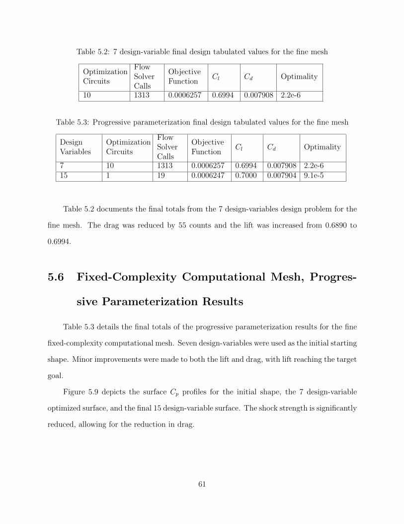
Table 5.2: 7 design-variable final design tabulated values for the fine mesh
OptimizationCircuits
FlowSolverCalls
ObjectiveFunction
Cl Cd Optimality
10 1313 0.0006257 0.6994 0.007908 2.2e-6
Table 5.3: Progressive parameterization final design tabulated values for the fine mesh
DesignVariables
OptimizationCircuits
FlowSolverCalls
ObjectiveFunction
Cl Cd Optimality
7 10 1313 0.0006257 0.6994 0.007908 2.2e-615 1 19 0.0006247 0.7000 0.007904 9.1e-5
Table 5.2 documents the final totals from the 7 design-variables design problem for the
fine mesh. The drag was reduced by 55 counts and the lift was increased from 0.6890 to
0.6994.
5.6 Fixed-Complexity Computational Mesh, Progres-
sive Parameterization Results
Table 5.3 details the final totals of the progressive parameterization results for the fine
fixed-complexity computational mesh. Seven design-variables were used as the initial starting
shape. Minor improvements were made to both the lift and drag, with lift reaching the target
goal.
Figure 5.9 depicts the surface Cp profiles for the initial shape, the 7 design-variable
optimized surface, and the final 15 design-variable surface. The shock strength is significantly
reduced, allowing for the reduction in drag.
61

Figure 5.9: Initial and final Cp profiles for 7 and 15 design variables
5.7 Adaptive Mesh Refinement
Initially, the test case was attempted using isotropic cells for the mesh adaption. It was
found that this would lead to a cell volume of 5e-13 for the first cell for a y+ value of 1
and a total number of surface mesh points of over 2 million. This mesh size is impractical
for the application of most CFD codes. Since this research was restricted to the use of
isotropic cell adaption, mesh adaption was not possible for this test case. There have been
preliminary attempts during this research of the application of anisotropic adaptive meshes
with cell aspect ratios of up to 100,000. While this is rather high, it does allow for much
better resolution of the boundary layer and the wake, with fewer cells. This appears to be
promising, as the mesh size is much closer to the size of the fine mesh for this research, which
is undersized as there is no wake for fine mesh and the y+ value of 1 is considered the upper
limit required for proper boundary layer resolution.
62

Chapter 6
Conclusions and Lessons Learned
6.1 Conclusions for Test Case 1
The current practice of using fixed-complexity computational meshes was found to be
more time efficient during the design process and to incur a lower user interaction penalty
compared to the use of loosely coupled AMR and optimization. This is true for the methods
employed in this research. The user interaction occurs through the toolbox setup within
FUN3D and could be reduced with scripting, but there will still be many more flow solver
calls with an adapted mesh refinement technique compared to the fixed-complexity compu-
tational mesh approach. This is due to the need to readapt the mesh at the end of each op-
timization circuit. Readaption is required as the shape change may cause the discretization-
error to increase in the mesh. A possible way to reduce this would be to use smaller bounds
so that the shape does not change as rapidly. This is not a typical case though, as most
design problems for real-world simulations will be starting from an already preliminary op-
timized shape, therefore the changes will typically be inherently small. Additionally, the
error estimates provided in the mesh refinement process may be used to help with the ever
increasing desire to apply statistical bounds to the solutions. This will help with certainty
63

in the final design before performing wind-tunnel testing and flight testing. One issue that
arose during this work for the adapted meshes is that the meshes tend to grow rapidly in
size when there are dramatic shape changes. One solution to alleviate this has been to try
smaller bounds. Meshes were observed to increase by an order of magnitude or more in size
in the presence of large shape changes, which adversely impacted the efficiency of the pro-
cess. It may be more efficient to perform many optimization circuits with smaller changes to
the design to help keep the mesh size down. An additional alternative method to maintain
smaller meshes sizes would be to perform progressive error tolerance with the loosely coupled
AMR approach.
6.2 Conclusions for Test Case 2
After the difficulties with the adaptive mesh refinement, and the under resolved coarse
and medium fixed-complexity computational meshes, this test case focused on documenting
and determining the best starting point for a previously optimized airfoil. A previously
optimized airfoil may be started with a relatively refined parameterization and achieve much
improvement for a relatively low cost. The shock is able to be reduced, which in turn
reduces the overall drag of the shape. However, one potential issue for transonic flight is the
creation of a single point-design airfoil that may be very ill-performing for other conditions.
To determine this, the shape should be tested at these other conditions and potentially
designed using multi-point optimization.
6.3 General Conclusions
Included are some general observations and conclusions from this research. The first is
that an increase in design-variables leads to a more optimal final shape. The second is that
64

the number of required flow solver calls increases with the number of design-variables and
with mesh complexity. Thirdly, it was found that bound settings can dramatically impact the
total cost. Too large bound settings may cause oscillations in the final shape, prolonging the
design process. Too small bound settings may require multiple reparameterizations during
the design process. Fourth, progressive parameterizations may reduce the number of flow
solver calls and the overall cost of the optimization. Fifth, progressive mesh complexity
reduces the number of flow solver calls and opens design optimization possibilities on the
more refined meshes that may have previously been deemed infeasible. A combination of
progressive mesh complexity and progressive parameterization leads to an even larger cost
reduction. Finally, AMR with design optimization reduces cost through mesh complexity
reduction, but there are cost increases due to the additional flow solver calls for the AMR
and the user interaction is doubled for each optimization circuit due to the current FUN3D
workflow.
6.4 Operational Lessons Learned
6.4.1 Fully converging the flow solution and adjoint solution
One of the most critical lessons learned from this research is that the flow solution and
adjoint solution must be fully converged for consistent optimization results. Fully converged
solutions enable the optimizer to better approximate the Hessian for the optimization. If this
is not done, the optimization tends to oscillate, and the optimizer will exit after reporting
numerical difficulties. To ensure the flow solver can converge more fully at each step, the
bounds must also be tightened on the design variables for the optimizer. Tightened bounds
limit the ability of the shape to change, therefore avoiding the introduction of shape changes
that disrupt the flow and in turn make the solution more amenable to convergence. Figure 6.1
illustrates a case when the flow solution does not achieve convergence. The output solution
65

for the adjoint and for the optimizer is now dictated by where the solution is stopped within
this unsteady behavior. The effect of tightening the bounds on the design space has not
been completely determined, and is recommended for future work.
Figure 6.1: Unconverged residuals
6.4.2 Fully converging mesh movement problem
One of the early limiting factors on the inflation of the bounds was the development
of negative cell volumes during mesh movement. Fully converging the mesh movement
problem to machine zero helped remove many of the negative cell volumes that arose during
large shape changes. By doing this, the optimization can perform the changes with fewer
optimization circuits. Potentially the same solution can be reached with the smaller bounds,
but this requires many more optimization circuits and increases the time dramatically.
6.4.3 Tightening bounds
Like the flow solution problem above, occasionally the design-variable value will oscil-
late within the bound limits during an optimization circuit. This causes the optimizer to
constantly adjust the design-variable, never converging to a solution, until it hits the major
iteration limits prescribed by the user. For example, during this research one particular case
called the flow solver over 1500 times and the optimizer was only adjusting the thickness
66

of the shape by 1e-4 or less. Since the optimizer could make the changes and there was
a difference in the solution, the optimizer continued to try to improve the design until the
major iteration limit was reached. Slightly tightening the bounds can remove this behavior,
and the design optimizer can converge to a solution in more than order of magnitude or fewer
flow solver calls. Figure 6.2 gives a comparison on the same starting point of an airfoil. The
loose bounds condition had bounds of 0.01 and the tight bounds test had bounds of 0.005.
Halving the bounds reduced the number of flow solutions by over 1400, while producing the
same final answer of 0.003621. This is different from the problem of not fully converging the
flow solver; these are both fully converged within the flow solver, but when the optimizer
slightly adjusts the shape, the overall optimization problem cannot converge.
(a) Loose bounds (b) Tight bounds
Figure 6.2: Bound limit comparison
6.4.4 Isotropic Mesh Adaption
Since the adapted meshes for this thesis are limited to isotropic cells, the adaption
presented is infeasible for a viscous flow case due to the computational tools used. FUN3D
has anisotropic mesh adaption capabilities but these were not used for this research. The
main limiting factor is the adaption toolbox itself. It is still a serial mesh adaption tool,
which means that memory overhead is an issue. The memory overhead due to the required
67

number of surface nodes to resolve the boundary layer and maintain isotropic cells exceeds
the ability to continue calculations. In future work, invoking the anisotropic adaptive mesh
refinement capability within FUN3D should enable this work to become feasible for 2D
viscous flow problems.
6.4.5 Restart vs Uniform start for design problems
All cases in the research presented here were performed with restarts between each
reparameterization. The initial restart is generated by running FUN3D’s flow solver and
saving the restart file, which is flagged to be saved within the input namelist. A new restart
file is saved at the end of each optimization cycle within an optimization circuit and used as
the initial conditions for the next optimization cycle. Restarts between parameterizations
are achieved by modifying FUN3D to read in a restart file each time. Restarts were not used
during the progressive fixed-complexity mesh research, as the meshes were increasing in size
and the flow solution was not able to be interpolated onto the new finer mesh. Restarts
were used during the adaption process by starting the process from the second cycle, which
uses the restart from the previous iteration during the adaption process. This allowed for a
single continuous restart file chain during the adaption process. This change was made after
early work showed a discrepancy between the final solution, obtained using a restart file and
the solution obtained starting with uniform flow initial conditions for the reparameterized
geometry. This difference was seen because the solution initialized with uniform flow was
not always able to reach a machine precision converged solution after a reparameterization.
More work needs to be done in this area, as both cases should provide the same solution,
whether starting from a restart or uniform flow initial conditions.
68

6.4.6 Bound Limits on Adapted Meshes
As mentioned in the conclusions to the first test case, future work should include re-
search concerning the magnitude of bounds allowed for adaptive meshing cases. This is
recommended as a result of the observation that some cases led to the generation of very
large meshes based on the specified error criteria when large shape changes were requested
by the optimizer.
6.5 Recommendations for Future Work
From this research, adaptive mesh refinement appears to provide a way to improve upon
design optimization cases for final values. While it may be more computationally expensive
currently with the large amount of user interaction required for performing adaptive mesh
refinement and design optimization within the FUN3D framework, developments can be
made to reduce this interaction and automate much of these processes. A progressive AMR
error tolerance is recommended for future work to determine if there are potential benefits,
similar to the benefits observed in the progressive mesh complexity cases performed in this
work
Future work recommendations include the use of anisotropic cells in the mesh refinement
process. This will allow for even further reduced mesh sizes. A potential issue with highly
stretched cells can be that smaller bounds may be required to prevent the occurrence of
negative volumes. Another recommendation is to incorporate global optimization schemes
into the initial design optimization process to help narrow the design space, after which
local optimization schemes may be used to finish optimizing the shape. As the adapted
meshes provide the user with error estimates, these estimates may be useful for uncertainty
quantification (UQ) during the design process. UQ is becoming an ever increasing desire
for design optimization as it allows for realistic bounds to be placed on values, helping to
69

improve the certainty of the design before production begins. Moving the adaption and
design optimization to three-dimensional problems is also recommended moving forward,
allowing for more true and realistic shapes to be developed for both wind tunnel testing and
flight testing.
70

Appendix A
Numerical Approach Figures
71

Initial Mesh
Flow Solver
Adjoint Solver
Error Esitmation
Mesh Adaption
New Mesh
Exit Criteria Met Exit
no
yes
Figure A.1: Computational mesh adaption process within FUN3D
Initial Mesh
Flow Solver
Adjoint Solver
Optimizer
Shape Change
Mesh Movement
New Shape
Exit Criteria Met Exit
no
yes
Figure A.2: Design optimization process within FUN3D
72

Initial Mesh
Design Optimization
New Shape
Mesh Adaption
New Mesh
Exit Criteria Met Exitno
yes
Figure A.3: Optimization then adaptation
Initial Mesh
Mesh Adaption
New Mesh
Design Optimization
New Shape
Exit Criteria Met Exitno
yes
Figure A.4: Adaption then optimization
73

Bibliography
[1] Li, D. and Hartmann, R., “Adjoint-Based Error Estimation and Mesh Refinement in anAdjoint-Based Airfoil Shape Optimization of a Transonic Benchmark Problem,” Noteson Numerical Fluid Mechanics and Multidisciplinary Design, Vol. 132, 2016, pp. 537–546.
[2] “AIAA Aerodynamic Design Optimization Discussion Group,”https://info.aiaa.org/tac/ASG/APATC/AeroDesignOpt-DG/default.aspx.
[3] Anderson, G. R., Nemec, M., and Aftosmis, M. J., “Aerodynamic Shape OptimizationBenchmarks with Error Control and Automatic Parameterization,” AIAA 2015-1719,53rd AIAA Aerospace Sciences Meeting, Kissimmee, FL January 2015.
[4] “CART3D Software,” https://www.nas.nasa.gov/publications/software/docs/cart3d/pages/cart3Dhome.html.
[5] Park, M. A., Anisotropic Output-Based Adaptation with Tetrahedral Cut Cells for Com-pressible Flows , Ph.D. thesis, Massachusetts Institute of Technology, September 2008.
[6] Jameson, A., “CFD for Aerodyanmic Design and Optimization: Its Evolution over theLast Three Decades,” AIAA 2003-3438, 16th AIAA Computational Fluid DynamicsConference, Orlando, FL June 2003.
[7] Jameson, A., “Efficient Aerodyanmic Shape Optimization,” AIAA 2004-4369, 10thAIAA/ISSMO Multidisciplinary Analysis and Optimization Conference, Albany, NYAugust 2004.
[8] Vassberg, J. C. and Jameson, A., “Aerodynamic Shape Optimization Part I: TheorticalBackground,” Lecture 1, Von Karman Institute, 2006.
[9] Vassberg, J. C. and Jameson, A., “Industrial Applications of Aerodynamic Shape Op-timization,” Lecture 2, Von Karman Institute, 2014.
[10] Mavriplis, D. J., “A Discrete Adjoint-Based Approach for Optimization Problems onThree-Dimensional Unstructured Meshes,” AIAA 2006-0050, 44th AIAA Aerospace Sci-ences Meeting and Exhibit, Reno, NV January 2006.
74

[11] Poole, D., Allen, C., and Rendall, T., “A Constrained Global Optimization Frame-work,” AIAA 2014-2034, 14th AIAA Aviation Technology, Integration, and OperationsConference, Atlanta, GA June 2014.
[12] Poole, D., Allen, C., and Rendall, T., “Comparison of Local and Global ConstrainedAerodynamic Shape Optimization,” AIAA 2014-3223, 32nd AIAA Applied Aerodynam-ics Conference, Atlanta, GA June 2014.
[13] Buckley, H. P., Zhou, B. Y., and Zingg, D. W., “Airfoil Optimization Using PracticalAerodynamic Design Requirements,” Journal of Aircraft , Vol. 47, No. 5, September-October 2010, pp. 1707–1719.
[14] Samareh, J. A., “Survey of Shape Parameterization Techniques for High-Fidelity Mul-tidisciplinary Shape Optimization,” AIAA Journal , Vol. 39, No. 5, 2001, pp. 877–884.
[15] Vassberg, J. C. and Jameson, A., “Influence of Shape Parameterization on AerodynamicShape Optimization,” Lecture 3, Von Karman Institute, 2014.
[16] Samareh, J., “Multidisciplinary aerodynamic-structural shape optimization using defor-mation (MASSOUD),” AIAA 2000-4911, 8th Symposium on Multidisciplinary Analysisand Optimization, Long Beach, CA September 2000.
[17] Castonguay, P. and Nadarajah, S. K., “Effect of Shape Parameterization on Aerody-namic Shape Optimization,” AIAA 2007-59, 45th AIAA Aerospace Sciences Meetingand Exhibit, Reno, NV January 2007.
[18] Mousavi, A., Castonguay, P., and Nadarajah, S. K., “Survey of Shape ParameterizationTechniques and its Effect on Three-Dimnesional Aerodynamic Shape Optimization,”AIAA 2007-3837, 18th AIAA Computational Fluid Dynamics Conference, Miami, FLJune 2007.
[19] Anderson, G., Aftosmis, M., and Nemec, M., “Parametric Deformation of Discrete Ge-ometry for Aerodynamic Shape Design,” AIAA 2012-0965, 50th AIAA Aerospace Sci-ences Meeting including the New Horizons Forum and Aerospace Exposition, Nashville,TN, January 2012.
[20] “Blender,” https://www.blender.org.
[21] Anderson, G. R. and Aftosmis, M. J., “Adaptive Shape Control for Aerodynamic De-sign,” NAS NAS-2015-02, NASA Ames Research Center, 2015.
[22] Park, M. A., Krakos, J. A., Michal, T., Loseille, A., and Alonso, J. J., “UnstructuredGrid Adaption: Status, Potential Impacts, and Recommended Investments Toward CFDVision 2030,” AIAA 2016-3323, 46th AIAA Fluid Dynamics Conference, Washington,DC June 2016.
75

[23] Slotnick, J., Khodadoust, A., Alonso, J., Darmofal, D., Gropp, W., Lurie, E., andMavriplis, D., “CFD Vision 2030 Study: A Path to Revolutionary Computational Aero-sciences,” NASA-CR-218178, March 2014.
[24] Venditti, D. A. and Darmofal, D. L., “Grid Adaption for Functional Outputs: Applica-tion to Two-Dimensional Inviscid Flows,” Journal of Computational Physcis , Vol. 176,2002, pp. 40–69.
[25] Venditti, D. A. and Darmofal, D. L., “Anisotropic grid adaptation for functional out-puts: application to two-dimensional viscous flows,” Journal of Computational Physcis ,Vol. 187, February 2003, pp. 22–46.
[26] Nemec, M. and Aftosmis, M. J., “Output Error Estimates and Mesh Refinement inAerodyanmic Shape Optimization,” AIAA 2013-865, 51st AIAA Aerospace SciencesMeeting including the New Horizons Forum and Aerospace Exposition, Dallas, TXJanuary 2013.
[27] Dalle, D. J. and Fidkowski, K. J., “Multifidelity Airfoil Shape Oprimization UsingAdaptive Meshing,” AIAA 2014-2996, 32nd AIAA Applied Aerodynamics Conference,AIAA AVIATION Forum, Atlanta, GA June 2014.
[28] Heath, C. M., Gray, J. S., Park, M. A., Nielsen, E. J., and Carlson, J.-R., “AerodynamicShape Optimization of a Dual-Stream Supersonic Plug Nozzle,” AIAA 2015-1047, 53rdAIAA Aerospace Sciences Meeting, Kissimmee, FL January 2015.
[29] Becker, R., Kapp, H., and Rannacher, R., “Adaptive Finite Element Methods for Op-timal Control of Partial Differential Equations: Basic Concept,” SIAM Journal onControl and Optimization, Vol. 39, No. 1, 2000, pp. 113–132.
[30] Becker, R. and Rannacher, R., “An optimal control approach to a posteriori errorestimation in finite element methods,” Acta Numerica, Vol. 10, 5 2001, pp. 1–102.
[31] Becker, R., “Mesh Adaption for Stationary Flow Control,” Journal of MathematicalFluid Mechanics , Vol. 3, 2001, pp. 317–341.
[32] Becker, R. and Vexler, B., “Optimal control of the convection-diffusion equation usingstabilized finite element methods,” Numerische Mathematik , Vol. 106, No. 3, 2007,pp. 349–367.
[33] Dede’, Luca, Q. and Alfio, “Optimal control and numerical adaptivity for advection–diffusion equations,” ESAIM: Mathematical Modelling and Numerical Analysis -Modelisation Mathematique et Analyse Numerique, Vol. 39, No. 5, 2005, pp. 1019–1040.
[34] Hintermuller, M. and Hoppe, R. H. W., “Goal-Oriented Adaptivity in Control Con-strained Optimal Control of Partial Differential Equations,” SIAM Journal on Controland Optimization, Vol. 47, No. 4, 2008, pp. 1721–1743.
76

[35] Li, R., Liu, W., Ma, H., and Tang, T., “Adaptive Finite Element Approximation forDistributed Elliptic Optimal Control Problems,” SIAM Journal on Control and Opti-mization, Vol. 41, No. 5, 2002, pp. 1321–1349.
[36] Micheletti, S. and Perotto, S., “The Effect of Anisotropic Mesh Adaptation on PDE-Constrained Optimal Control Problems,” SIAM Journal on Control and Optimization,Vol. 49, No. 4, 2011, pp. 1793–1828.
[37] Yan, N. and Zhou, Z., “A priori and a posteriori error analysis of edge stabilizationGalerkin method for the optimal control problem governed by convection-dominated dif-fusion equation,” Journal of Computational and Applied Mathematics , Vol. 223, No. 1,2009, pp. 198 – 217.
[38] Pointwise, “Pointwise V17,” http://www.pointwise.com/pw/.
[39] Gill, P. E., Murray, W., and Saunders, M. A., “SNOPT: An SQP Algorithm for Large-Scale Constrained Optimization,” SIAM Review , Vol. 47, No. 1, 2005, pp. 99–131.
[40] Hicken, J. E. and Zingg, D. W., “Aerodynamic Optimization Algorithm with IntegratedGeometry Parameterization and Mesh Movement,” AIAA Journal , Vol. 48, No. 2,2017/04/17 2010, pp. 400–413.
[41] Biedron, R. T., Carlson, J.-R., Derlaga, J. M., Gnoffoo, P. A., Hammond, D. P., Jones,W. T., Kleb, B., Lee-Rausch, E. M., Nielsen, E. J., Park, M. A., Rumsey, C. L.,Thomas, J. L., and Wood, W. A., “FUN3D Manual: 12.9,” NASA TM-2016-219012,Langley Research Center, February 2016.
[42] Spalart, P. R. and Allmaras, S. R., “A One-Equation Turbulence Model for Aerody-namic Flows,” La Recherche Aerospatiale, Vol. 1, No. 1, 1994, pp. 5–21.
[43] “K-Cluster,” http://k-info.larc.nasa.gov/CCFresources hardware.html, October 2013.
[44] Spalart, P. R., “Extensions of d’Alembert’s paradox for elongated bodies,” Tech. Rep.2181, The Royal Society, 2015.
[45] Hartmann, R., “PADGE DG solver from Center for Computer Applications inAeroSpace Science and Engineering,” http://www.dlr.de/as/en/desktopdefault.aspx/,2006, Electronic Software.
[46] Milholen, W. E. and Owens, L. R., “On the Application of Contour Bumps for Tran-sonic Drag Reduction (Invited),” Conference Proceedings 462, American Institute ofAeronautics and Astronautics, January 2005.
[47] Campbell, R., “Efficient viscous design of realistic aircraft configurations,” AIAA 1998-2539, 29th AIAA, Fluid Dynamics Conference, Albuquerque, NM June 1998.
[48] Owens, L., “Private Correspondence,” Discussion on TMA-0712 Airfoil.
77