To the Graduate Council:

I am submitting herewith a dissertation written by Niranjan Anandrao Patil entitled “Field Weakening Operation of AC Machines for Traction Drive Applications.” I have examined the final electronic copy of this dissertation for form and content and recommend that it be accepted in partial fulfillment of the requirements for the degree of Doctor of Philosophy, with a major in Electrical Engineering.

J. S. Lawler

Major Professor

We have read this dissertation and recommend its acceptance:

L. M. Tolbert

S. M. Djouadi

Suzanne Lenhart

Accepted for the Council:

Carolyn R. Hodges Vice Provost and Dean of the Graduate School

(Original Signatures are on file with official student records)

Field Weakening Operation of AC

Machines for Traction Drive

Applications

A Dissertation

Presented for the

Doctor of Philosophy Degree

The University of Tennessee, Knoxville

Niranjan Anandrao Patil

August 2009

ii

Dedication

This dissertation is dedicated to my parents, Anandrao and Padma; my sister, Swarada;

and my wife, Neha, for always believing in me, inspiring and encouraging me to reach

higher in order to achieve my goals.

iii

Acknowledgements

I want to thank Dr. Jack Lawler for continuously providing me with invaluable knowledge

and guidance, Drs. John McKeever and Leon Tolbert for providing me a research

assistantship at Oak Ridge National Laboratory, my department for providing a teaching

assistantship, Pedro Otaduy for sharing SRM data with me which was necessary for the

nonlinear analysis of SRM motor. I would also like to thank Cliff White, Matthew

Scudiere and Chester Coomer for their help at the National Transportation Research

Center and I would like to thank Dr. S. M. Djouadi and Dr. Suzanne Lenhart for serving

on my committee. Finally, I would like to thank my parents; my sister; my wife; my in-

laws, Medha, Arvind and Abhay; and my friends, Rahul, Pushkar, Asim, Anindyo and

Weston, for their unending support and encouragement.

iv

Abstract

The rising cost of gasoline and environmental concerns have heightened the interest in

electric/hybrid-electric vehicles. In passenger vehicles an electric traction motor drive

must achieve a constant power speed range (CPSR) of about 4 to 1. This modest

requirement can generally be met by using most of the common types of electric

motors. Heavy electric vehicles, such as tanks, buses and off-road equipment can

require a CPSR of 10 to 1 and sometimes much more. Meeting the CPSR requirement

for heavy electric vehicles is a significant challenge. This research addresses the

CPSR capability and control requirements of two candidates for high CPSR traction

drives: the permanent magnet synchronous motor (PMSM) and the switched reluctance

motor (SRM).

It is shown that a PMSM with sufficiently large winding inductance has an infinite CPSR

capability, and can be controlled using a simple speed control loop that does not require

measurement of motor phase currents. Analytical and experimental results confirm that

the conventional phase advancement method charges motor winding with required

current to produce the rated power for the speed range where the back-EMF normally

prevents the generation of the rated power. A key result is that for the PMSM, the motor

current at high speed approaches the machine rating independent of the power

produced. This results in poor partial load efficiency.

v

The SRM is also shown to have infinite CPSR capability when continuous conduction is

permitted during high speed operation. Traditional high speed control is of

discontinuous type. It has been shown that this discontinuous conduction itself is the

limiter of CPSR. Mathematical formulas have been developed relating the average

current, average power, and peak current required producing the desired (rated) power

to machine design parameters and control variables. Control of the SRM in the

continuous conduction mode is shown to be simple; however, it does require

measurement of motor current. For the SRM the motor current at high speed is

proportional to the power produced which maintains drive efficiency even at light load

conditions.

vi

TABLE OF CONTENTS

1 INTRODUCTION .................................................................................................................................. 1

1.1 ELECTRICAL OR HYBRID ELECTRICAL TRANSPORTATION VEHICLES .................................................. 1

1.2 INTRODUCTION TO FIELD WEAKENING ............................................................................................. 3

1.3 VIABLE CANDIDATES FOR FIELD WEAKENING OPERATION ................................................................ 6

1.4 DISSERTATION OBJECTIVES AND OUTLINE ....................................................................................... 8

2 LITERATURE REVIEW: PERMANENT MAGNET SYNCHRONOUS MOTORS ............................. 13

2.1 FIELD WEAKENING OPERATION OF PERMANENT MAGNET SYNCHRONOUS MOTORS ........................ 15

2.1.1 Constant Voltage Constant Power Vector Control [8],[29] .................................................... 27

2.1.2 Constant Current Constant Power Vector Control [19] [30] .................................................. 30

2.1.3 Optimum Current Vector Control [9] ...................................................................................... 32

3 CONVENTIONAL PHASE ADVANCEMENT METHOD ................................................................... 37

3.1 ANALYSIS OF A PERMANENT MAGNET SYNCHRONOUS MOTOR DRIVEN BY CONVENTIONAL PHASE

TIMING ADVANCEMENT METHOD [37]. ........................................................................................................ 40

3.1.1 Fundamental Frequency Model............................................................................................. 44

3.1.2 Below Base Speed Operation (Constant Torque Zone, n≤1) ............................................... 48

3.1.3 Operation above Base Speed (Constant Power Region, n≥1) ............................................. 50

3.1.4 “Optimal” Inductance for the Field-Weakening ...................................................................... 53

3.2 STEADY STATE PMSM CONTROL CONSIDERING WINDING RESISTANCE ......................................... 56

3.2.1 Constant Power Speed Ratio ................................................................................................ 61

4 SIMULATIONS AND EXPERIMENTAL VERIFICATION OF CONVENTIONAL PHASE

ADVANCEMENT METHOD FOR SURFACE PM MACHINES. ................................................................. 63

4.1 SIMULINK BASED SIMULATION MODEL ........................................................................................... 63

4.2 SIMULATION RESULTS .................................................................................................................. 70

4.3 MEASURED MACHINE DATA .......................................................................................................... 72

vii

4.4 EXPERIMENTAL SETUP ................................................................................................................. 75

4.5 EXPERIMENTAL RESULTS AND CONCLUSION ................................................................................ 102

5 INTRODUCTION – SWITCHED RELUCTANCE MOTORS ............................................................ 132

5.1 MODELING OF SWITCHED RELUCTANCE MOTORS [4][51]. ............................................................ 137

6 LITERATURE REVIEW – SWITCHED RELUCTANCE MOTOR CONTROL ................................. 148

6.1.1 Low Speed Voltage Control (Voltage PWM)[15],[59] .......................................................... 151

6.1.2 Low Speed Current Control [15],[59] ................................................................................... 153

6.1.3 High Speed Single Pulse Control of Switched Reluctance Motors ..................................... 154

6.2 LITERATURE REVIEW – HIGH SPEED SINGLE PULSE CONTROL ..................................................... 158

7 CONTINUOUS CONDUCTION ANALYSIS AND SIMULATION RESULTS ................................. 177

7.1 EXAMPLE MOTOR MODEL ........................................................................................................... 178

7.1.1 Nomenclature and Parameters of the Example Motor ........................................................ 181

7.2 EXAMPLE MOTOR ANALYSIS ....................................................................................................... 183

7.2.1 Linear Model ........................................................................................................................ 184

7.2.2 Nonlinear Model .................................................................................................................. 185

7.2.3 Nonlinear Model with Partial Derivatives ............................................................................. 191

7.2.4 Nonlinear Model with Current Estimation from Flux-Linkage Data ..................................... 191

7.3 SIMULATION RESULTS ................................................................................................................ 194

7.4 CONTINUOUS CONDUCTION ANALYSIS - FLAT UNALIGNED INDUCTANCE TYPE SRM ....................... 205

7.4.1 Region I Analysis ( 0 ( )r a ) ........................................................................ 211

7.4.2 Region II Analysis ( ( )r a ) ....................................................................... 213

7.4.3 Region III Analysis (

2*

2* 2*

r dwell r

r dwell

) ................................................ 214

7.4.4 Region IV Analysis ( 2* 2*r dwell r ) ........................................... 215

viii

7.4.5 Region V Analysis ( r r commutation ) ............................................... 215

7.4.6 Region VI Analysis ( r commutation r ) ......................................................... 216

7.4.7 Analytical Results ................................................................................................................ 219

7.4.8 Validation of Analytical Results ........................................................................................... 233

7.4.9 Controller Analysis .............................................................................................................. 240

7.4.10 Constant Power Speed Ratio .......................................................................................... 253

7.5 CONTINUOUS CONDUCTION ANALYSIS - NON-FLAT UNALIGNED INDUCTANCE ................................ 256

7.5.1 Region I Analysis ( 0 ( )r adv ) ...................................................................... 264

7.5.2 Region II Analysis ( ( )r adv ) ..................................................................... 266

7.5.3 Region III Analysis ( r dwell ) ........................................................................ 267

7.5.4 Region IV-a Analysis ( 2

rr dwell

) ................................................................... 268

7.5.5 Region IV-b Analysis (2

rdwell

) .............................................................................. 269

7.5.6 Region V Analysis ( dwell r ) ......................................................................... 270

7.5.7 Region VI Analysis (

r r commutation

r r dwell adv

)............................................ 271

7.5.8 Region VII Analysis ( r commutation r ) ........................................................ 272

7.5.9 Analytical Results ................................................................................................................ 274

7.5.10 Validation of Analytical Results (Simulation Results) ..................................................... 285

7.5.11 Controller Analysis .......................................................................................................... 300

7.5.12 Constant Power Speed Ratio .......................................................................................... 304

8 CONCLUSION AND FUTURE WORK ............................................................................................ 309

8.1 SURFACE PERMANENT MAGNET SYNCHRONOUS MOTOR ............................................................. 309

ix

8.2 SWITCHED RELUCTANCE MOTOR ................................................................................................ 312

Bibliography ............................................................................................................................................ 316

Appendix .................................................................................................................................................. 330

Vita ............................................................................................................................................................ 362

x

LIST OF TABLES

Table 2-1: Torque Equations [24] .................................................................................. 20

Table 4-1: Parameters of a Surface Permanent Magnet Synchronous Motor with

Fractional-Slot Concentrated Windings. ........................................................................ 64

Table 4-2 : Machine per-phase Resistance and per-phase Inductance Measurement. 74

Table 4-3 : Measured No Load Losses and Machine Data. .......................................... 80

Table 4-4 : 250V, 25% Load ........................................................................................ 104

Table 4-5 : 250V, 50% Load ........................................................................................ 105

Table 4-6 : 250V, 75% Load ........................................................................................ 106

Table 4-7: 250V, 100% Load ....................................................................................... 107

Table 4-8 : 300V, 25% Load ........................................................................................ 108

Table 4-9 : 300V, 50% Load ........................................................................................ 109

Table 4-10 : 300V, 75% Load ...................................................................................... 110

Table 4-11 : 300V, 100% Load. ................................................................................... 111

Table 4-12 : Current Comparison at 250V and 300V DC. ........................................... 119

Table 4-13 : Minimum Current and Unity Power Factor Speed. .................................. 128

Table 4-14 : Calculated Torque Component of the Stator Current (with 300V DC). .... 130

Table 7-1 : Flat Unaligned Inductance type SRM, Dwell = 31. .................................... 236

Table 7-2 : Flat Unaligned Inductance type SRM, Dwell = 31. .................................... 237

Table 7-3 : Flat Unaligned Inductance type SRM, Dwell = 31. .................................... 238

Table 7-4: Flat Unaligned Inductance type SRM, Dwell = 32. ..................................... 239

Table 7-5 : Peak Current Required to get Rated Power. ............................................. 248

xi

Table 7-6 : Rated Power Development at High Speed. ............................................... 248

Figure 7-28 : CPSR Analysis – Flat Unaligned Inductance type SRM. ....................... 254

Table 7-7: CPSR of the Flat Unaligned Inductance type SRM with Discontinuous

Conduction. ................................................................................................................. 257

Table 7-8 : Non-flat Unaligned Inductance type SRM, Dwell = 31° (Linear Model and

Non Linear Model). ...................................................................................................... 288

Table 7-9 : Non-flat Unaligned Inductance type SRM Dwell = 31° (Linear Model). ..... 289

Table 7-10: Non-flat Unaligned Inductance type SRM Dwell = 31° (Non Linear Model).

.................................................................................................................................... 290

Table 7-11 : Non-flat Unaligned Inductance type SRM Dwell = 31° (Linear Model). ... 291

Table 7-12: Non-flat Unaligned Inductance type SRM Dwell = 31° (Non Linear Model).

.................................................................................................................................... 292

Table 7-13 : Current Regulator Set Point to get Rated Power. .................................... 297

Table 7-14 : Rated Power at High Speed using Continuous Conduction. ................... 298

Table 7-15 : CPSR of the Non Flat Unaligned Inductance type SRM with Discontinuous

Conduction. ................................................................................................................. 308

xii

LIST OF FIGURES

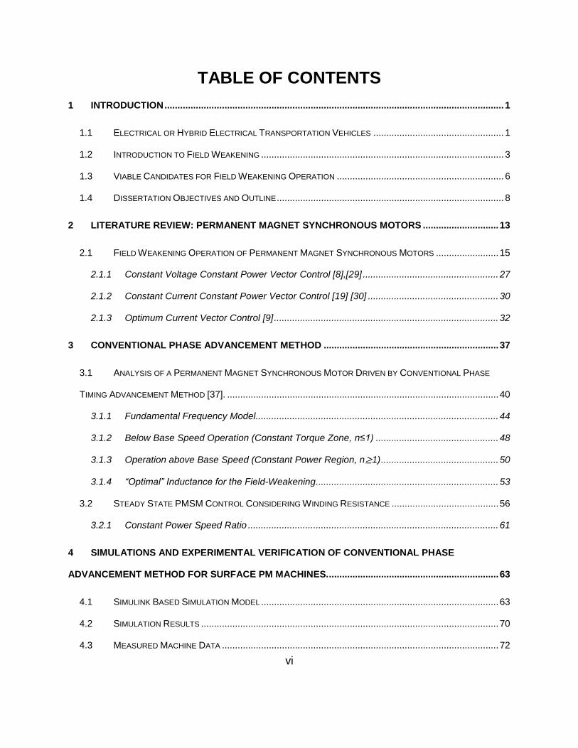
Figure 1-1: Typical AC Drive Characteristics. ................................................................. 2

Figure 1-2 : Electrical Equivalent Circuit of a Separately Excited DC Motor. ................... 4

Figure 1-3: AC Motor Classification Based on the Shape of Back EMF Waveform. ....... 7

Figure 2-1: Surface Permanent Magnet Motor - Cross Sectional View. ........................ 14

Figure 2-2: Interior Permanent Magnet Motor - Cross Sectional View. ......................... 16

Figure 2-3: Synchronous Reluctance Motor - Cross Sectional View. ........................... 17

Figure 2-4: Electrical Equivalent d-q Circuit of a Synchronous Motor in the

Synchronously Rotating Reference Frame [23]. ............................................................ 20

Figure 2-5: Current and Voltage Limited Operation of Permanent Magnet Motors [8]. . 23

Figure 2-6: Below Base Speed Operation of Surface PM Machines [28]. ..................... 26

Figure 2-7: Above Base Speed Operation of Surface PM Machines [8][9]. ................... 28

Figure 2-8: Constant Current Constant Power Vector Control. ..................................... 31

Figure 2-9: Optimum Current Vector Control. ................................................................ 33

Figure 2-10: Scheme of Flux-Weakening Control System for Permanent Magnet

Synchronous Motors [9]. ............................................................................................... 34

Figure 2-11: Optimal Condition for Flux Weakening Operation of Surface PM Motors

[31]. ............................................................................................................................... 35

Figure 3-1: Comparison of Back-EMF and Applied Stator Voltage above Base Speed

without Field-Weakening. .............................................................................................. 38

Figure 3-2: Comparison of Back EMF and Applied Voltage above Base Speed With

Phase Advancement. .................................................................................................... 39

xiii

Figure 3-3: Motor / Inverter Schematic for a PMSM Driven by CPA [37]. ...................... 41

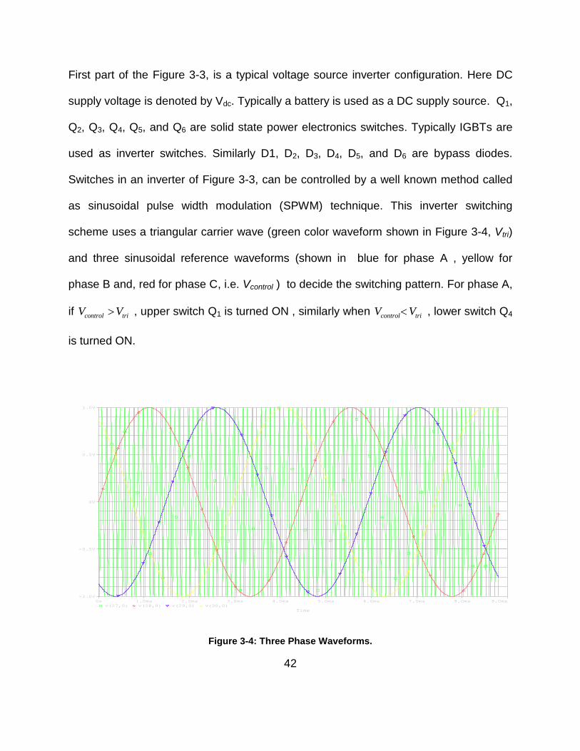
Figure 3-4: Three Phase Waveforms. ........................................................................... 42

Figure 3-5: Fundamental Frequency Model. ................................................................. 45

Figure 3-6: Vector Diagram of Conventional Phase Advancement Method. ................. 57

Figure 4-1: Simulink Model for CPA driven PMSM Simulation. ..................................... 65

Figure 4-2 : PMSM Motor Model ................................................................................... 68

Figure 4-3 : Vehicle Dynamics. ..................................................................................... 69

Figure 4-4 : Simulation Results for CPA driven PMSM motor at Full Load (6kW) and 151

Vdc Supply Voltage. ....................................................................................................... 71

Figure 4-5: No Load Losses Measurement Setup. ........................................................ 73

Figure 4-6 : Per Phase Stator Winding Inductance Measurement using LCR meter. .... 74

Figure 4-7 : Measured Back-EMF of a 6-kW Fractional-Slot Concentrated-Winding

PMSM Motor at Base Speed (900 rpm). ....................................................................... 76

Figure 4-8 : Measured Back-EMF of a 6-kW Fractional-Slot Concentrated-Winding

PMSM Motor at 4000 rpm. ............................................................................................ 77

Figure 4-9 : Measured Back-EMF with FFT at Base Speed (900 rpm).......................... 78

Figure 4-10 : Measured Back-EMF with FFT at 1800 rpm. ........................................... 79

Figure 4-11: Measured No Load Losses of a 6-kW Fractional-Slot Concentrated-

Winding Motor. .............................................................................................................. 81

Figure 4-12 : Measured Back-EMF of a 6-kW Fractional-Slot Concentrated-Winding

PMSM Motor. ................................................................................................................ 82

Figure 4-13: Close up of the Experimental 6-kW Surface PM Motor. ............................ 83

xiv

Figure 4-14 : Index Pulse from Incremental Encoder on back-EMF at 900 rpm. ........... 85

Figure 4-15: Rotor Position Estimation. ......................................................................... 87

Figure 4-16 : Overall Electrical Schematics. .................................................................. 88

Figure 4-17 : a. Motor & Dyne Coupling, b. Voltage & Current Sensors........................ 90

Figure 4-18 : Overall Experimental Setup. .................................................................... 91

Figure 4-19 : Overall Test Schematics. ......................................................................... 92

Figure 4-20 : Simulink Based OPAL RT Model. ............................................................ 96

Figure 4-21: Data Acquisition and Motor Control (OPAL RT Model). ............................ 97

Figure 4-22: Part of the CPA Based Controller for Surface PM Motor with Fractional-Slot

Concentrated Windings. ................................................................................................ 98

Figure 4-23 : Modulation Index and Inverter Lead Angle Logic. .................................. 100

Figure 4-24: Details of the Sine Triangle type PWM Switching Scheme. .................... 101

Figure 4-25 : Data Monitor (OPAL RT). ....................................................................... 103

Figure 4-26 : Speed Tracking. ..................................................................................... 112

Figure 4-27: Measured Power Vs Speed, Torque Vs Speed and Current Vs Speed for

300V, & 100% Load. ................................................................................................... 114

Figure 4-28: Measured Losses. ................................................................................... 115

Figure 4-29 : Measure Inverter Efficiency. ................................................................... 117

Figure 4-30 : Measured Motor Efficiency. .................................................................... 118

Figure 4-31 : Measured Drive Efficiency. .................................................................... 121

Figure 4-32 : Comparison of Inverter Efficiency. ......................................................... 122

Figure 4-33 : Comparison of Motor Efficiency. ............................................................ 123

xv

Figure 4-34 : Comparison of Total Drive Efficiency. .................................................... 124

Figure 4-35: No Load Losses and Drive Efficiencies. .................................................. 126

Figure 5-1 : Cross-Sectional View of a Four Phase 8/6 Switched Reluctance Motor. . 133

Figure 5-2: Asymmetrical Half-Bridge Voltage Source Inverter Topology for an 8/6 SRM

Motor [11],[15]. ............................................................................................................ 135

Figure 5-3: Per Phase Equivalent Circuit of Switched Reluctance Motor. ................... 139

Figure 5-4: Per Phase Inductance Profile of an 8/6 SRM Motor (Neglecting Saturation).

.................................................................................................................................... 141

Figure 5-5: Flux-Linkage Vs Current Plot. ................................................................... 145

Figure 6-1: Firing Scheme of an 8/6 SRM Motor. ........................................................ 149

Figure 6-2: Voltage Control (Voltage PWM) [59]. ........................................................ 152

Figure 6-3: Current Type SRM Control. ....................................................................... 155

Figure 6-4: Single Pulse High Speed Operation of SRM Motors. ................................ 157

Figure 6-5: Speed Control System for Switched Reluctance Motor Based on [65]. .... 162

Figure 6-6: Inner Torque Control Loop for Switched Reluctance Motor based on [65].

.................................................................................................................................... 163

Figure 6-7: Closed Loop High Speed Control Scheme for Switched Reluctance Motor

Based on [12],[11]. ...................................................................................................... 165

Figure 6-8: Current Regulator Set Point as a Function of Output Torque [11]. ............ 166

Figure 6-9: Advance Angle Estimation [11]. ................................................................ 168

Figure 6-10: High Speed SRM Control Based on [11]. ................................................ 169

xvi

Figure 6-11: Closed Loop Torque Control Loop for Continuous Conduction Based on

[75]. ............................................................................................................................. 175

Figure 7-1: Flux-Linkage Vs Rotor Position Plot for the Example SRM Motor. ............ 179

Figure 7-2: Flux-Linkage Vs Current plot for the Example Motor. ............................... 180

Figure 7-3: Example Motor Data. ................................................................................ 182

Figure 7-4: Maximum Co-Energy of the Example Motor with Peak Current of 600A. .. 183

Figure 7-5: Linear Magnetic Model of the Example Motor. .......................................... 186

Figure 7-6: Linear Inductance Profile of the Example Motor. ...................................... 187

Figure 7-7: Simulink Model for the Example Motor [ L(θ) ]. ........................................ 188

Figure 7-8: Inductance Profile of the Example SRM. .................................................. 189

Figure 7-9: Simulink Model for the Example Motor Simulation [ L(θ,i) ]. ...................... 190

Figure 7-10: Partial Derivatives for Nonlinear Model. .................................................. 192

Figure 7-11: Simulink Model Based on Partial Derivatives. ......................................... 193

Figure 7-12: Simulink Model of the Example Motor based on Current Estimation from

Flux-Linkage Data. ...................................................................................................... 195

Figure 7-13: Instantaneous Phase Current and Co-energy for the Example Motor when

Producing Rated Power at Base Speed [78]. .............................................................. 196

Figure 7-14: : Instantaneous Phase Current and Co-energy for the Example Motor when

Producing Rated Power at 6 Times Base Speed (using model in Section 7.2.2). ....... 197

Figure 7-15: Simulation Result of Discontinuous Conduction: Advance Angle = 22.5 ,

Dwell = 30, Iset = 600A @ 6500 RPM (using model in 7.2.2). .................................... 200

xvii

Figure 7-16: Simulation Result of Continuous Conduction: Advance Angle = 22.5 , Dwell

= 31, Iset = 600A @ 6500 RPM (using model in Section 7.2.2). ................................. 201

Figure 7-17 : Continuous conduction (n = 6, dwell = 31°, advance angle = 22.5°, and

Ipeak = 600A). ............................................................................................................. 202

Figure 7-18: Inductance Profile Comparison for Linear Model and Non-Linear Model.204

Figure 7-19: Location of Zero Volt-Sec Notches for Flat Unaligned Inductance type SRM

Motor when Operated in Continuous Conduction (Matlab Simulation). ....................... 206

Figure 7-20: Flat Unaligned Inductance type SRM Analysis when Operated in

Continuous Conduction. .............................................................................................. 207

Figure 7-21: Validation of Flat Unaligned Inductance Type SRM Motor Analysis, Speed

= 6500 rpm (n=26), Dwell = 31°, Advance Angle = 23° and Current Regulator Set Point,

Ipeak = 600A. .............................................................................................................. 234

Figure 7-22 : Comparison Between Analytical and Simulation Results. ...................... 241

Figure 7-23 : Comparison Between Analytical and Simulation Results. ...................... 242

Figure 7-24 : Comparison Between Analytical and Simulation Results. ...................... 243

Figure 7-25 : Comparison Between Analytical and Simulation Results. ...................... 244

Figure 7-26 : Dwell Angle Vs Advance Angle (Speed = 3750 RPM, Ipeak = 500A). ... 245

Figure 7-27: Power Control in Continuous Conduction Mode. .................................... 247

Figure 7-28 : CPSR Analysis – Flat Unaligned Inductance type SRM. ....................... 254

Figure 7-29 : Non-Flat Unaligned Inductance Profile................................................... 258

Figure 7-30 : Notch Location for Non Flat Unaligned Inductance type SRM when

Operated in Continuous Conduction Mode. ................................................................ 260

xviii

Figure 7-31 : Continuous Conduction Analysis – Non Flat Unaligned Inductance type

SRM. ........................................................................................................................... 261

Figure 7-32: Validation of Non-flat Unaligned Inductance Type SRM Motor Analysis,

Speed = 3750 rpm (n=15), Dwell = 31° , Advance Angle = 23° and Current Regulator

Set Point, Ipeak = 600A. ............................................................................................. 286

Figure 7-33 : Average Power. ..................................................................................... 287

Figure 7-34: Comparison of Analytical Results with Simulation Results for a Non Flat

Unaligned Inductance Profile type SRM Motor. ........................................................... 294

Figure 7-35 : Comparison of Analytical and Simulation Results. ................................. 295

Figure 7-36 : Comparison of Analytical and Simulation Results. ................................. 296

Figure 7-38 : Comparison between Non Linear and Linear Analysis for Rated Output

Power. ......................................................................................................................... 299

Figure 7-39: Dwell Angle Vs Advance Angle (Speed = 3750 RPM, Ipeak = 500A). .... 301

Figure 7-40 : Power Control in Continuous Conduction Mode. ................................... 302

Figure 7-41 : Response to a Step Change in Current Regulator Set when Operating at

6500 RPM with Dwell Angles of 30.25o and 31o. ......................................................... 303

Figure 7-42: CPSR Estimation with Single Pulse High Speed Operation of the Non flat

Unaligned Inductance type SRM. ................................................................................ 305

xix

Abbreviations

RMS = Root Mean Square

EMF = Electro-Motive Force

PM = Permanent Magnet

IPM = Interior Permanent Magnet Motor

SPM = Surface Permanent Magnet Motor

IM = Induction Motor

PMSM = Permanent Magnet Synchronous Motor

CPSR = Constant Power Speed Ratio

SPWM = Sinusoidal Pulse Width Modulation

CPA = Conventional Phase Advancement Method

SRM = Switched Reluctance Motor

PI = Proportional + Integral type Controller

DC = Direct Current

1

1 INTRODUCTION

1.1 Electrical or Hybrid Electrical Transportation Vehicles

Air pollution concerns, oil dependence on politically unstable regions and high oil prices

are some of the reasons that have caused a flurry of activity in the areas of efficient

electrical or hybrid electrical vehicles. If only an internal combustion engine is used,

application of brakes results into generation of heat energy (kinetic energy gets

converted into heat energy). If an electric motor or a combination (motor and an internal

combustion engine) is used, kinetic energy can be converted into regenerative power

which can be used to recharge batteries. This improves overall vehicle efficiency. The

selection of a particular motor technology depends on several factors like cost,

efficiency, size, weight, noise level etc. Locomotives are a good example of a high

starting torque requirement. When a train is started, it is typically accelerated with a

rated torque to a constant coasting speed. Once it reaches this cruising speed, low but

sufficient torque to overcome road losses is required. Occasionally, the train may be

required to run at a much higher speed than the designed cruising speed. These

desired characteristics of a traction vehicle fit well with a motor having a wide speed

range. Many other applications such as fork-lifts, golf carts, excavators, dump trucks,

construction vehicles, and mining shovels also require high torque at low speeds and

higher speed range. Other examples of traction vehicles are various types of

construction trucks. They require not only high torque capability but also high speed

2

operation, particularly when driving on state or interstate highways. With current

technology, at low speed, most of the electrical drives can be controlled to produce high

torque. Special control technique has to be applied in order to operate electrical traction

vehicles at high speed. There are several reasons for this limited speed range. One of

the reasons is the upper limits that are placed on the motor input voltage and motor

current due to the limitation on available DC supply voltage (battery). Power electronics

used in the voltage source inverter which converts this DC voltage in an AC voltage,

also puts some limitations on voltage and current capacity. These limits not only restrict

the maximum torque but also the maximum speed at which rated power can be

produced. Figure 1-1 shows ideal as well as practical drive characteristics. In traction

vehicle terminology, base speed ( bn ) or the rated speed is the speed at which available

motor input voltage (or inverter output voltage) will be at the maximum value.

Figure 1-1: Typical AC Drive Characteristics.

Speed Maximum Speed

Constant Torque Region O

utp

ut P

ow

er

Real Drive

Ideal Drive

CPSR

Constant Power Region

Rated Power

Base Speed

3

Below this speed is the constant torque region. Above base speed, starts a constant

power region.

AC drives do not have a natural flat output power characteristic at high speed. As the

speed increases, output power increases. Once the applied voltage is at the maximum

value, output power starts to decrease. At some speed, developed power drops below

the rated power of the motor. The ratio of this highest speed at which the rated power

can be developed to the base speed is called Constant Power Speed Ratio (CPSR) [1].

Widely used vector controlled induction motor drives can offer a CPSR of 4:1[1]. The

next section describes a typical control scheme used to extend the high speed range of

a separately excited DC motor.

1.2 Introduction to Field Weakening

Separately excited DC motors, if controlled properly, can provide ideal Torque / Power

characteristics. To illustrate this, consider the steady state electrical model of a

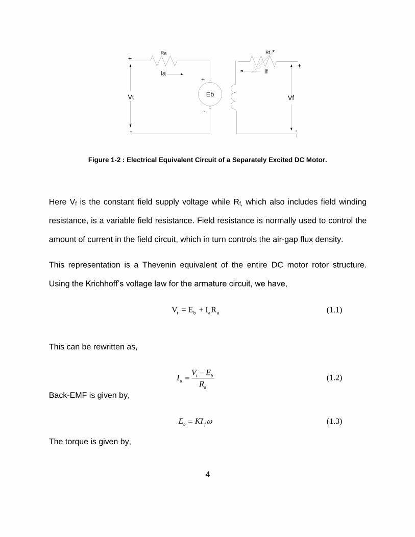
separately excited DC motor, as shown in Figure 1-2. . In this model, the armature

circuit is represented by an ideal terminal supply voltage source Vt, winding resistor Ra,

and generated back-EMF Eb. The back-EMF is generated due to the interaction

between the armature circuit magnetic flux and the field circuit magnetic flux. In this type

of an electrical motor, the air gap flux density is provided by the electromagnets which

are energized by the controllable field current If.

4

Eb

Ra

++

--

Vt Vf

IfIa

Rf

+

-

Figure 1-2 : Electrical Equivalent Circuit of a Separately Excited DC Motor.

Here Vf is the constant field supply voltage while Rf, which also includes field winding

resistance, is a variable field resistance. Field resistance is normally used to control the

amount of current in the field circuit, which in turn controls the air-gap flux density.

This representation is a Thevenin equivalent of the entire DC motor rotor structure.

Using the Krichhoff’s voltage law for the armature circuit, we have,

t b a aV = E + I R (1.1)

This can be rewritten as,

t ba

a

V EI

R

(1.2)

Back-EMF is given by,

b fE KI (1.3)

The torque is given by,

5

e t f aT = K * I * I (1.4)

Here = motor speed in rad/sec, and Kt, Kg are the motor design constants (torque and

back EMF respectively). From Equation (1.4), it is clear that, in constant torque region,

to keep the torque constant, field current If and the armature current Ia have to be kept

constant or their product has to be maintained constant. If can be held constant by

keeping field supply voltage Vf and field winding resistance Rf constant. From Equation

(1.2) , armature current Ia depends on the difference between the motor terminal voltage

Vt and back-EMF Eb. As shown in Equation (1.3) , Eb increases with speed due to its

dependence on motor speed . Thus the converter output voltage must be increased to

keep the armature current constant to keep the toque constant till base speed. At low

speed, the rated armature current and the rated excitation flux can be used to obtain the

rated motor torque. Because there is a limit on the available DC supply voltage, at some

speed Nb, also called the base speed or the rated speed, the converter will reach its

limiting output voltage Vt max. Above this base speed, only way force the current into the

motor is by reducing the back-EMF. From Equation(1.3), this can be done by reducing

the field current If. In this region, output torque through its dependence on the field

current and the armature current will also decrease with increase in the speed, i.e.,

1

T

(1.5)

Since Output Power, e eP = T (1.6)

6

Above base speed, the process of producing the rated power by lowering the air gap

flux density (field flux f = K If ) to increase the speed range of an electrical motor is

termed as the “flux weakening” or the “field weakening”.

1.3 Viable Candidates for Field Weakening Operation

Basic principles of electromagnetic induction were discovered in the early 1800's by

Oersted, Gauss, and Faraday. By 1820, Hans Christian Oersted and Andre Marie

Ampere had discovered that an electric current can produce a magnetic field. The next

15 years saw a flurry of cross-Atlantic experimentation and innovation, leading finally to

a simple DC rotary motor. While experimenting in 1834, Thomas Davenport developed

what we today know as a DC motor, complete with a brush and commutator (receiving

U.S. Patent No. 132). After the development of the Ward Leonard system of Control [2]

(Patent No. 463,802), DC motors became the motor of choice for loads that require

precise control of speed and torque. The Induction Motor (IM) was invented by Nikola

Tesla in 1888 [3]. His landmark paper in AIEE (May 15th, 1888) was entitled “A New

Alternating Current Motor”. Once the concept of a “cage” was introduced, it was an easy

step to the development of synchronous motors. The earliest recorded Switched

Reluctance Motor (SRM) was one built by Davidson in Scotland in 1838 [4]. It did not

become viable until the recent developments in high power switching devices such as

Bipolar Junction Power Transistor (BJT) in the early 1980’s. The development of Alnico

magnets by Bell Laboratories in the 1930’s triggered the development of Permanent

7

Magnet (PM) machines. In 1950’s ceramic magnets became available. In 1960’s

commercial rare earth PMs became available. At present, neodymium-iron-boron

(NdFeB) magnets are used for traction drive application. To aid in the choice of the field

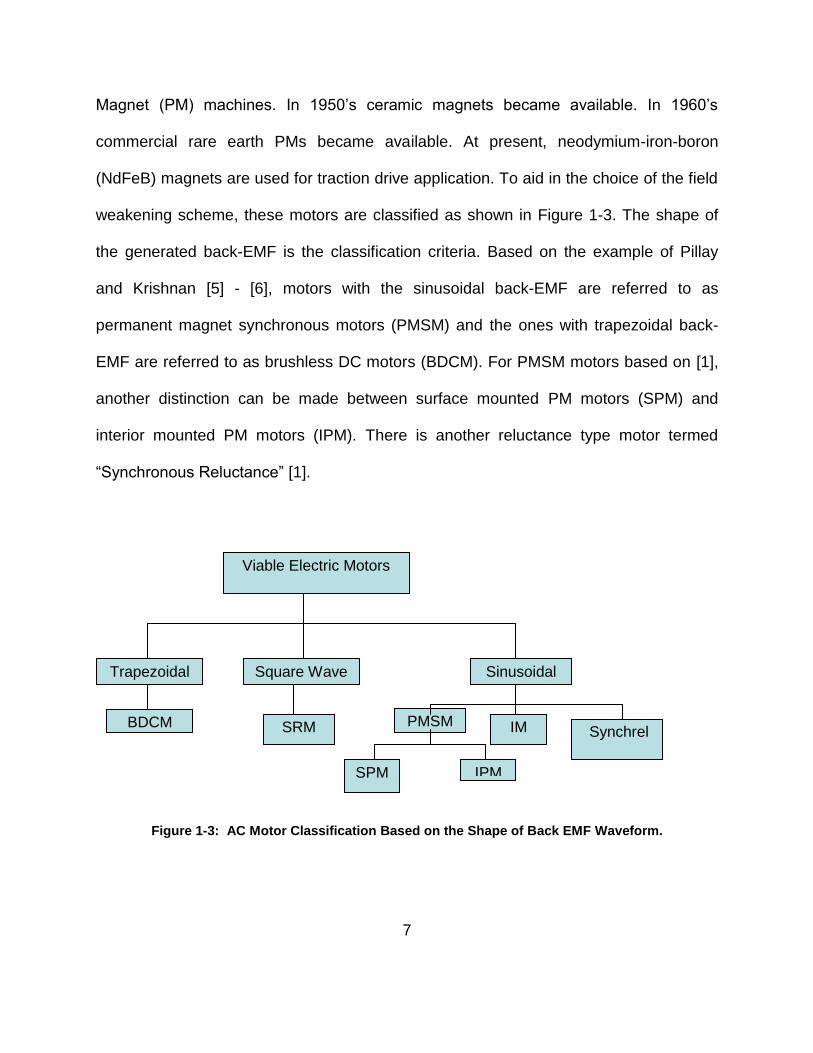
weakening scheme, these motors are classified as shown in Figure 1-3. The shape of

the generated back-EMF is the classification criteria. Based on the example of Pillay

and Krishnan [5] - [6], motors with the sinusoidal back-EMF are referred to as

permanent magnet synchronous motors (PMSM) and the ones with trapezoidal back-

EMF are referred to as brushless DC motors (BDCM). For PMSM motors based on [1],

another distinction can be made between surface mounted PM motors (SPM) and

interior mounted PM motors (IPM). There is another reluctance type motor termed

“Synchronous Reluctance” [1].

Figure 1-3: AC Motor Classification Based on the Shape of Back EMF Waveform.

Viable Electric Motors

Trapezoidal Square Wave Sinusoidal

BDCM SRM PMSM

SPM IPM

IM Synchrel

8

Only induction motors have a controllable source of air gap flux density like that of a DC

motor. The well-studied equivalent circuit of an induction motor can be used to derive

the analytical expressions for its CPSR [7]. Analysis has shown that the induction motor

does not have a natural “constant power” operating region [7]. During field weakening

operation, when producing as much power as possible within the current rating of the

motor, power output monotonically decreases with speed. The rate of decrease of

developed power is related to drive parameters and indicate that several factors may

reduce the rate of decrease of power with speed during field weakening [7]. The

formulas indicate that while many model parameters influence the CPSR to some

extent, it is the maximum permissible magnetizing current magnitude, DC supply

voltage, base speed and torque requirement, and leakage inductances that have the

greatest effect [7]. In situations where the motor design is fixed, the only parameters

that can be varied by the drive designer are the DC supply voltage and power rating.

This puts limits on the CPSR and prevents the use of a widely used induction motor for

traction drive applications requiring a CPSR of 10:1 or more. In this research, the

Surface Permanent Magnet Synchronous Motor and Switched Reluctance Motor have

been considered for traction drive applications requiring a wide CPSR (10:1 or more).

1.4 Dissertation Objectives and Outline

The overall objective of this research was to increase the highest speed at which PMSM

and SRM motors can produce their rated power without exceeding their current limits.

9

The rotor of the PMSM motor has surface permanent magnets resulting in smooth and

constant torque with high power density. Due to the use of permanent magnets,

permanent magnet synchronous motors have higher torque and higher efficiency [1], [8]

than that of induction motors for the same size. In case of separately excited DC

motors, there are two sets of windings resulting in “torque producing” and “field

producing” currents. These currents are controlled independently, and in the constant

power region, the field current is reduced to produce the rated power. In PMSM motors,

there is only a stator winding and field flux is produced by the permanent magnets. As

described in the Chapter 2, when the motor is in the constant power or field-weakening

region, a part of this stator current has to be used to weaken the field produced by these

permanent magnets and the remaining part of that current can produce the rated power.

Chapter 2 reviews vector control based field-weakening methods that are typically used

for the high speed operation of PMSM motors. These methods require an accurate

measurement of the stator current. For a three phase motor, this means the use of six

voltage and six current sensors. These measured currents and voltages are then

converted to the “field component” and the “torque component”. Above motor base

speed, the “field component” of the current is applied such that it opposes the magnetic

field produced by the permanent magnets.

If not used properly, this traditional “field weakening” method can cause irreversible

demagnetization of the rotor permanent magnets [9]. The need for three phase voltage

and current measurement results in more drive hardware size, weight and cost. The

three-phase to two-phase transformation means more mathematical complexity, slower

10

system response and more required computational power. Use of sensors also reduces

the reliability of the control system.

The primary goal for this part of the research was to develop a simple high speed

controller. For this research, a conventional phase advancement method was

considered as a field-weakening control scheme. Cambier et al have a patent on this

conventional phase advancement method for brushless DC motors [10]. Chapter 3

describes the adaptation of this CPA method for the surface permanent magnet

synchronous motors. This chapter also describes the development of a real time

controller based on this CPA method. A fundamental frequency model of PMSM motor

was considered for realizing this high speed controller.

It has been shown that three simple equations form the basis of this high speed

controller. Chapter 4 is focused on the implementation and experimental verification of

the CPA based control method to widen the CPSR ratio of a surface PM motors. It is

shown that with the CPA based controller, there is a well defined speed at which a

PMSM motor operates at a unity power factor. At this speed, the resultant current is at

the minimum value. Also, at this speed, the inverter efficiency is at its highest level. It is

possible to adjust the machine design parameters such that this minimum speed will be

the same as the nominal speed of the motor. Also, it has been shown that this CPA

based method does not require any phase voltage or current measurements. This

method does not require any three-phase to two-phase transformations, which reduces

complexity, hardware size and implementation cost.

11

When compared with induction motors or permanent magnet motors, switched

reluctance motors are simpler in design. The rotor of the SRM motor is nothing but a

stack of steel laminations, making SRM simple in construction and low in cost. As there

is no source of rotor excitation (permanent magnets or windings), SRMs are inherently

fault-tolerant [11], and they can be used in very high speed or high temperature

applications [12]. Use of a proper converter topology can avoid shoot-through faults and

isolate the faulted phase, eliminating a possibility of drag torque and fire hazard during

phase failure. In Chapter 6 and 7, it has been shown that this SRM structure results in a

higher natural CPSR than PMSM motors [13], but it also results in more torque

pulsation and acoustic noise. Therefore, the SRM is an ideal candidate for heavy off-

road vehicles where vibrations and noise are generally not an issue.

Traditional SRM control is of a discontinuous type. For example, at the beginning of

each cycle, the stator current starts from zero and returns back to zero. Chapter 6

reviews the existing constant torque and constant power region control strategies. In

Chapter 7, it has been shown that this discontinuous type high speed control strategy

itself is the limiter of the CSPR. Because of the non-linearity due to saturation and

complex interdependence of the winding inductance, current and flux-linkages, with

traditional discontinuous conduction, associated machine data is required to derive a

look up table relating required peak current and output torque [14] , [15]. This data is

typically obtained by FEA analysis or by carrying out a number of experiments. Even

though, an SRM motor is low cost and fault tolerant, designing an SRM controller is

tedious.

12

For this research, a continuous conduction based high speed control scheme has been

considered. Switched Reluctance Drives Limited has patents (US 5469039, US

5545964, US 5563488) on continuous type control schemes. The primary goal for the

second part of the research was to mathematically analyze the high speed operation of

SRM motors when continuous conduction is used. Chapter 7 describes this

mathematical analysis. It has been shown that if the speed-sensitive losses are ignored,

the CPSR of an SRM motor can be infinite when a continuous conduction based high-

speed control scheme is used [13] and the resultant average and RMS current are well

below the rated value. At high speed, saturation is not an issue [16]. Using a linear

magnetic model, analytical expressions have been derived relating resultant average

motor power and average motor current to the machine design and control parameters.

Analytical expressions relating required peak current to the desired output power have

also been derived. In Section 7.4 and Section 7.5, required residual flux-linkage and

resultant minimum current have been derived. For verification purposes, these

analytical results have been compared with simulation results based on linear as well as

non-linear models. In Chapter 7, it has been shown that the control variables required

for continuous conduction based control scheme are same as the low-speed,

discontinuous conduction based control scheme.

13

2 LITERATURE REVIEW: PERMANENT MAGNET SYNCHRONOUS MOTORS

Inverter driven permanent magnet synchronous motors (PMSM) are widely used in high

performance variable frequency drive systems. The stator of a typical synchronous

motor is the same as that of a standard induction motor (IM). It is made of a number of

stampings slotted to receive stator windings. Permanent magnet synchronous motors

also have sinusoidal flux distribution. This results in a sinusoidal back EMF and requires

sinusoidal currents to produce constant torque. Unlike induction motors, the rotor of a

synchronous motor has permanent magnets (PM) instead of electro-magnets. When

compared to an induction motor, these rare earth permanent magnets create high

density magnetic field. This results in higher efficiency and lighter weight [10]. Constant

magnetic field also generates relatively constant torque for a constant stator current

input [10]. This inherent characteristic of PMSM motors to produce a constant torque for

a constant current is considered to be a drawback for applications in electric vehicles.

Particularly in the constant power region, torque has to decrease with increase in speed

in order to produce the constant rated power without exceeding current rating. PMSM

motors also have higher power factor compared to that of an Induction Motor [5]. Figure

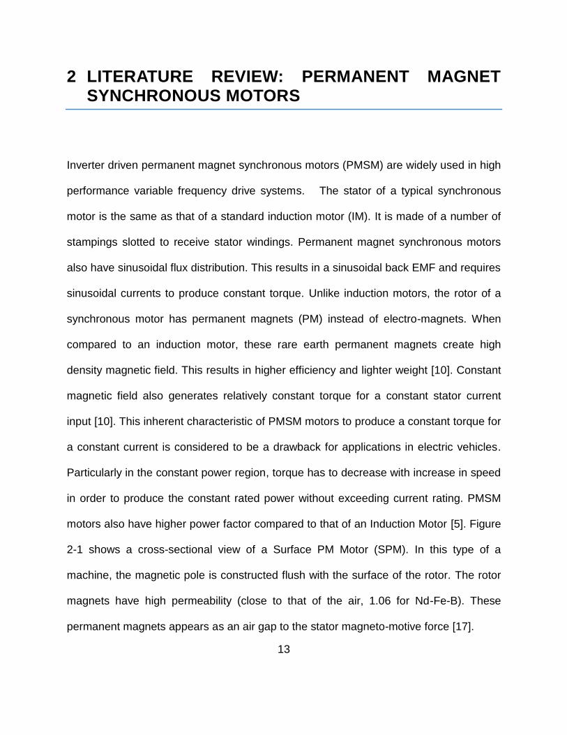
2-1 shows a cross-sectional view of a Surface PM Motor (SPM). In this type of a

machine, the magnetic pole is constructed flush with the surface of the rotor. The rotor

magnets have high permeability (close to that of the air, 1.06 for Nd-Fe-B). These

permanent magnets appears as an air gap to the stator magneto-motive force [17].

14

Air Gap

Stator Core

Rotor Core

Shaft – Non

Magnetic

Permanent

Magnets

Figure 2-1: Surface Permanent Magnet Motor - Cross Sectional View.

15

Therefore, the air gap flux density between the stator and the rotor is uniform hence

SPM is a non-salient type of machine. As a result only magnetic torque is produced.

The term salient means “protruding” or “sticking out” and a salient pole is a magnetic

pole that sticks out from the surface of the rotor. Figure 2-2 shows a cross sectional

view of an Interior Permanent Magnet motor (IPM). Here rotor magnets are inset into

the rotor. Here, the air gap flux density between stator and rotor is not uniform. As a

result both magnetic and reluctance torques are produced.

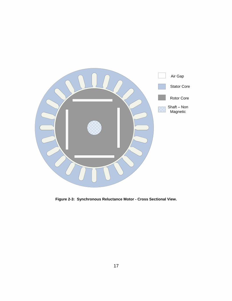
Figure 2-3 shows a cross sectional view of the synchronous reluctance motor. Here

rotor has air gaps. As a result only reluctance torque is produced.

2.1 Field Weakening Operation of Permanent Magnet Synchronous

Motors

Motors with sinusoidal operation can be characterized by parameters resolved into a

quadrature-axis and a direct-axis component. The problem arises due to the speed

dependency of machine inductances, whereupon the coefficients of differential

equations (voltage equations), which describe the motor behavior, are time varying

except when the motor is at standstill. After several configuration dependent

transformations were developed, it was recognized that there is one “general”

transformation which eliminates all time-varying inductances.

16

Air Gap

Stator Core

Rotor Core

Shaft – Non

Magnetic

Permanent

Magnets

Figure 2-2: Interior Permanent Magnet Motor - Cross Sectional View.

17

Air Gap

Stator Core

Rotor Core

Shaft – Non

Magnetic

Figure 2-3: Synchronous Reluctance Motor - Cross Sectional View.

18

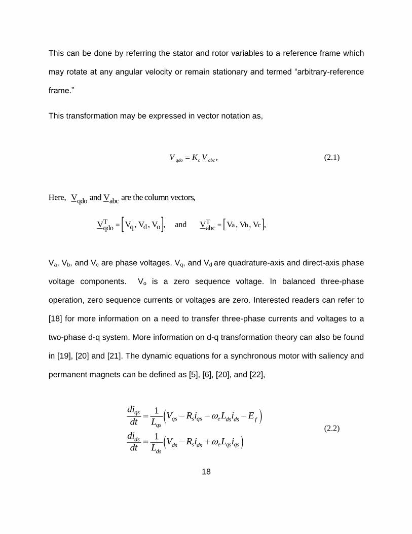
This can be done by referring the stator and rotor variables to a reference frame which

may rotate at any angular velocity or remain stationary and termed “arbitrary-reference

frame.”

This transformation may be expressed in vector notation as,

,qdo abcsV K V (2.1)

Here, V and V are the column vectorsqdo abc ,

V V V VqdoT

q d o , , , and V V V VabcT a b c , , ,

Va, Vb, and Vc are phase voltages. Vq, and Vd are quadrature-axis and direct-axis phase

voltage components. Vo is a zero sequence voltage. In balanced three-phase

operation, zero sequence currents or voltages are zero. Interested readers can refer to

[18] for more information on a need to transfer three-phase currents and voltages to a

two-phase d-q system. More information on d-q transformation theory can also be found

in [19], [20] and [21]. The dynamic equations for a synchronous motor with saliency and

permanent magnets can be defined as [5], [6], [20], and [22],

1

1

qsqs s qs e ds ds f

qs

dss e qs qsds ds

ds

diV R i L i E

dt L

diV R i L i

dt L

(2.2)

19

Here Rs= stator per phase winding resistance, Lqs=q-axis inductance, Lds= d-axis

inductance, Ef = back-EMF due to magnetic flux, e = electrical rotor speed, Vqs = q-axis

voltage component, Vds = d-axis voltage component, Iqs = q-axis current component, ids=

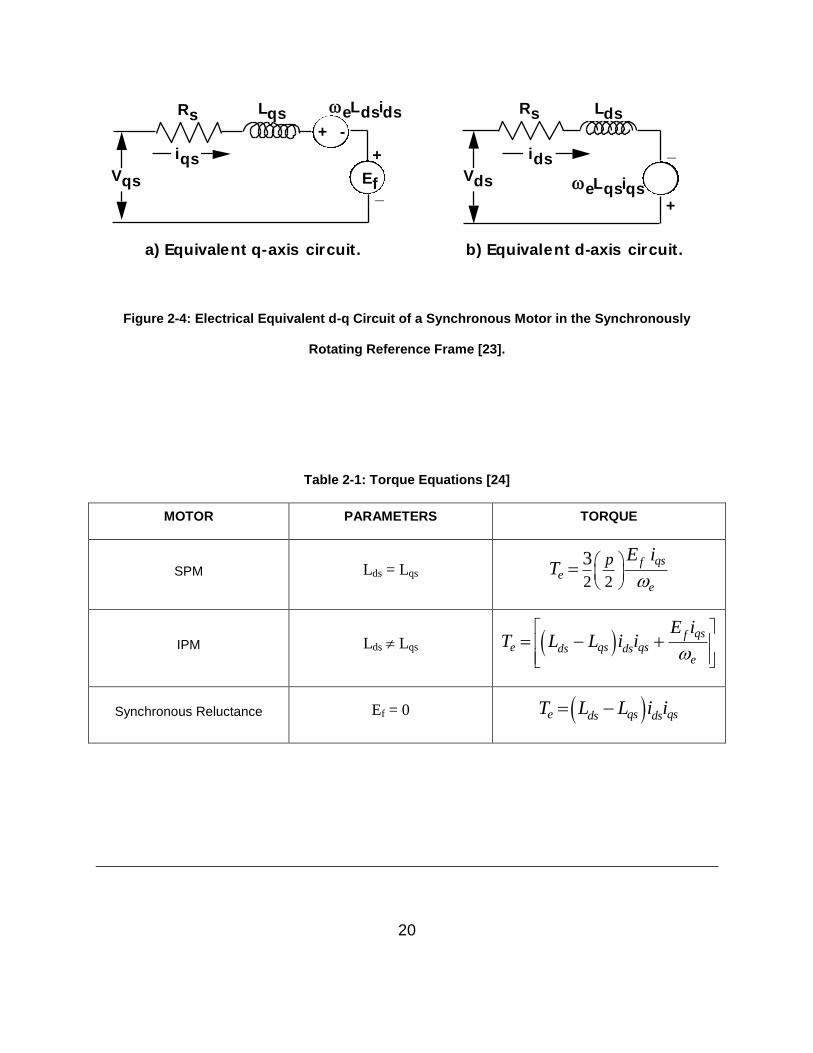
d-axis current component. Equation (2.2) is consistent with the circuit of Figure 2-4.

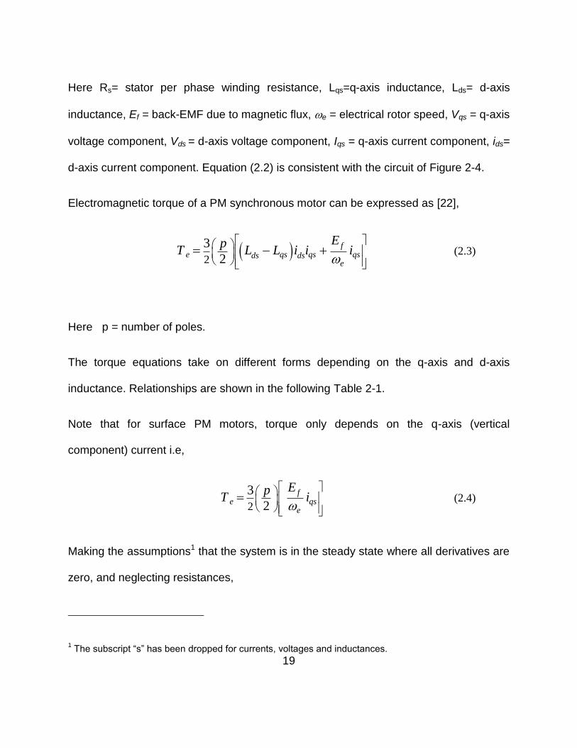
Electromagnetic torque of a PM synchronous motor can be expressed as [22],

2

3

2f

e qs qs qsds dse

EpT L L i i i

(2.3)

Here p = number of poles.

The torque equations take on different forms depending on the q-axis and d-axis

inductance. Relationships are shown in the following Table 2-1.

Note that for surface PM motors, torque only depends on the q-axis (vertical

component) current i.e,

2

3

2f

e qse

EpT i

(2.4)

Making the assumptions1 that the system is in the steady state where all derivatives are

zero, and neglecting resistances,

1 The subscript “s” has been dropped for currents, voltages and inductances.

20

Figure 2-4: Electrical Equivalent d-q Circuit of a Synchronous Motor in the Synchronously

Rotating Reference Frame [23].

Table 2-1: Torque Equations [24]

MOTOR PARAMETERS TORQUE

SPM Lds = Lqs 2 2

3 qsfe

e

p E iT

IPM Lds Lqs qsfe qs qsds ds

e

E iT L L i i

Synchronous Reluctance Ef = 0 e qs qsds dsT L L i i

iqs

+ -

Rs Lqs eLdsids

EfVqs

+ _

LdsRs

+_

eLqsiqsVds

a) Equivalent q-axis circuit. b) Equivalent d-axis circuit.

ids

21

Equation (2.2) now becomes

d e q qV L i (2.5)

And

q e d d fV L i E (2.6)

These voltages are subject to the voltage limitations due to the limitation on available

DC link voltage.

2 2 2

q d rV V V (2.7)

Similarly, the current limitations due to limitations of the power devices used in the

inverter system and winding insulations,

2 2 2

q d ri i I (2.8)

Here, Ir = rated stator current value in amperes and, Vr = rated stator voltage value in

volts.

Combining Equations (2.5) and (2.6), in Equation (2.7) , we have,

2 2

2

e q q e d d f rL i L i E V (2.9)

22

Defining, f

mag f

e

E

flux linkages due to rotor permanent magnets,

Equation (2.9) becomes,

2 2

1

mag

dqd

r r

d e q e

iiL

V V

L L

(2.10)

In the ,d qi i plane, Equation (2.10) is an ellipse centered at -

mag

Ld. With rated voltage Vr

fixed, this ellipse shrinks inversely with the speed of the motor, e. Thus, one has a

voltage-limit ellipse and a current-limit circle. We note that for the surface type

permanent magnet motors, Lq and Ld are equal (due to non-saliency). Thus, the

voltage-limit ellipse degenerates into a circle. The current limiting circle and the voltage

circle are shown in Figure 2-5 [9]. At = o any control action must occur within the

cross-hatched area. Below base speed, all the action occurs inside the current limiting

circle.

Above base speed, the applied voltage is the maximum and the back-EMF exceeds the

applied voltage. Consequently the back-EMF has to be reduced to produce torque in

the constant power region. Unlike separately excited DC motors or induction motors,

PM synchronous motors do not have a separate and controllable source of air-gap flux

density. Therefore, a component of the stator current (the d-axis current) must be used

to counter the air-gap flux density.

23

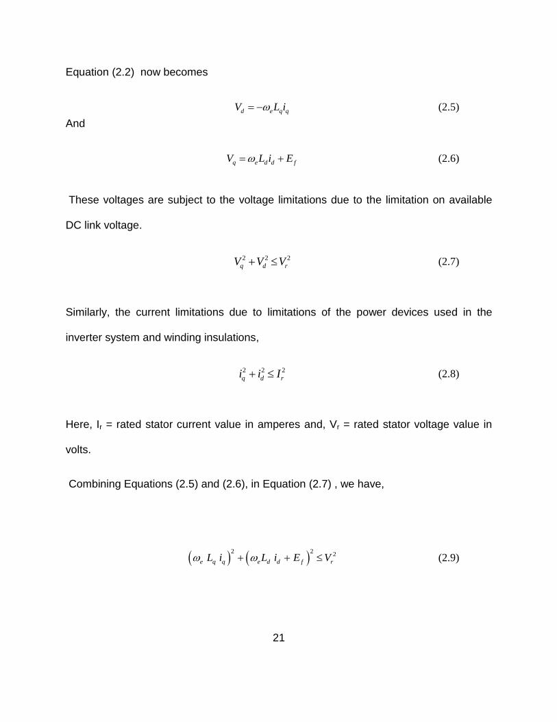
Figure 2-5: Current and Voltage Limited Operation of Permanent Magnet Motors [8].

qi

Current limiting circle

Voltage limiting circles

Increasing speed

0

di

24

The q-axis component of the stator current is then used to develop the required torque.

This has led to the terminology “flux-weakening” [8]. Controllers that control both the

magnitude and the phase angle of the stator excitation are termed as “vector

controllers” [25]. Since this “vector control” also results in the control of spatial

orientation of the electromagnetic field, the term “field orientation” [25] is also used. The

flux weakening control [8] is very useful for high speed, constant power operation

considering the voltage constraint. This is a desired characteristic in traction

applications. Since part of the current is “wasted” in field weakening, surface PM

machines have generally been considered to be poor candidates for achieving this wide

constant power speed [1].

The center of the voltage limiting circle in Equation (2.10) is also called as the

characteristic current of SPM machines, and is defined as,

mag

CH

d

IL

(2.11)

Here mag is the RMS magnetic flux linkage and dL is the d – axis inductance. This

center should lie inside the current limiting circle (red circle in Figure 2-5). Theoretically

SPM machines have infinite CPSR if CH ratedI I [26]. For surface PM machines, this

characteristic current is usually several times higher than the rated current of the

machine [8]. With conventional distributed stator winding, due to the large effective air

gap, inductance value of the SPM machines is typically low. Due to use of permanent

magnets, the magnet flux linkage is quite high. This results in much higher value of the

25

characteristic current than the rated current, putting limits on achievable CPSR. It is also

well known that when the rated current of the motor is equal to the characteristic current

of the motor, flux weakening is optimal [1]. For this reason a wider CPSR can simply be

achieved by a adding a series of external inductors [17]. This technique increases

weight, volume and losses [1]. Surface PM Machines with a fractional slot concentrated

windings (FSCW) have considerably higher inductance, mainly due to higher slot

leakage inductance [26], [27]. Surface PM Machines equipped with concentrated

windings provide the highest power and torque density [26] compared to that of

distributed windings. Due to the lower winding losses, FSCW machines also have

superior thermal performance in the constant power region [26]. Although, distributed

winding machines have the best inverter utilization. Without flux weakening, a machine

must be designed to produce the rated torque over the entire speed range. This also

requires over sizing of an inverter. Additionally, low inductance increases the switching

requirements of power devices and causes high short circuit currents.

The electric torque produced by the surface PM machine is given by[22],

2

3

2 mage q

pT i

Here mag is the flux produced by the permanent magnets and p is the number of stator

poles. For a given machine design, output torque only depends on the q-axis current. In

the constant torque region (below base speed operation), maximum torque-per-amp is

26

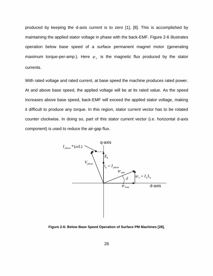
produced by keeping the d-axis current is to zero [1], [8]. This is accomplished by

maintaining the applied stator voltage in phase with the back-EMF. Figure 2-6 illustrates

operation below base speed of a surface permanent magnet motor (generating

maximum torque-per-amp.). Here a is the magnetic flux produced by the stator

currents.

With rated voltage and rated current, at base speed the machine produces rated power.

At and above base speed, the applied voltage will be at its rated value. As the speed

increases above base speed, back-EMF will exceed the applied stator voltage, making

it difficult to produce any torque. In this region, stator current vector has to be rotated

counter clockwise. In doing so, part of this stator current vector (i.e. horizontal d-axis

component) is used to reduce the air-gap flux.

Figure 2-6: Below Base Speed Operation of Surface PM Machines [28].

d-axis mag

gap

a q qI L

q phasei I

bE

phaseV

*( )phaseI L

q-axis

27

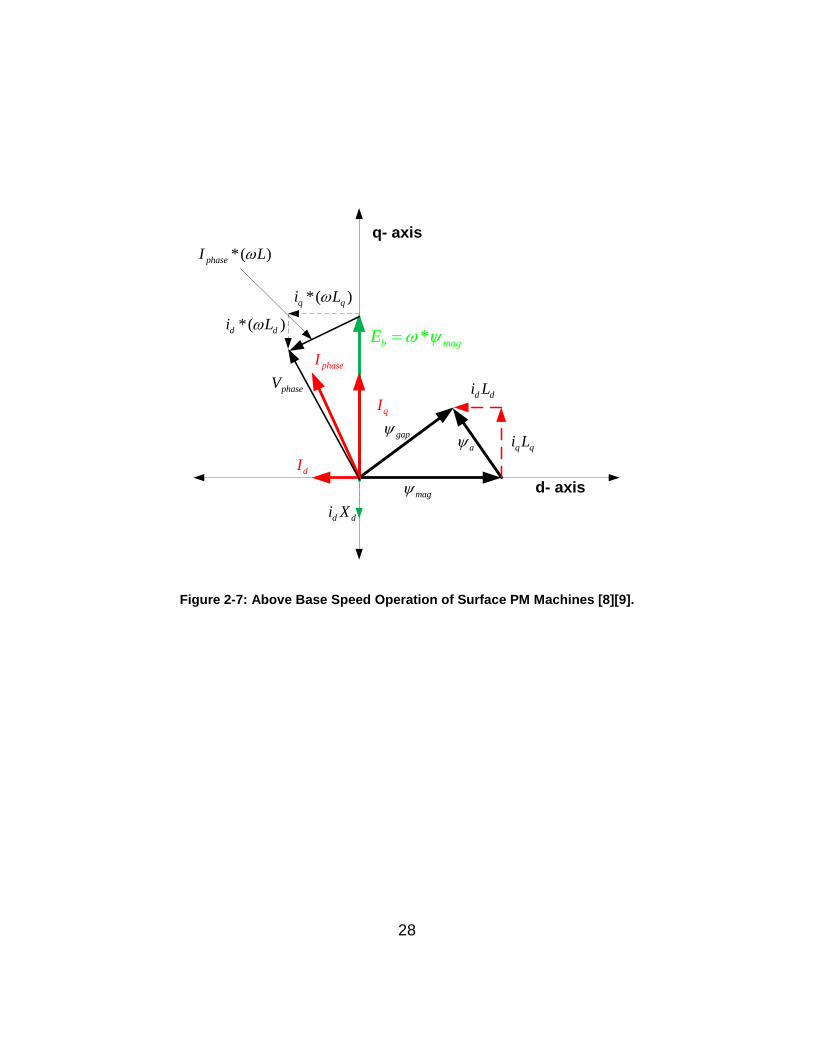
This in turn reduces the generated back-EMF. The remaining vertical or q-axis

component of the stator current is then used to produce the required torque. Figure 2-7

illustrates above base speed, field weakening operation of the Surface PM Machines.

As speed increases, current vector rotates more towards the direct-axis. At some

speed, developed torque becomes zero as all of the current is used to reduce the back-

EMF. In constant power zone, as the part of the current is used to oppose the magnetic

field produced by the permanent magnets, magnet demagnetization due to the direct

axis armature reaction must be prevented.

The demagnetization process is irreversible and it decreases the electro-magnetic

torque [9]. Use of magnets with large coercive force helps with the above problem in

field-weakening zone operation of permanent magnet synchronous motors [28]. The

following sections describe some of the available field weakening techniques for surface

PM machines.

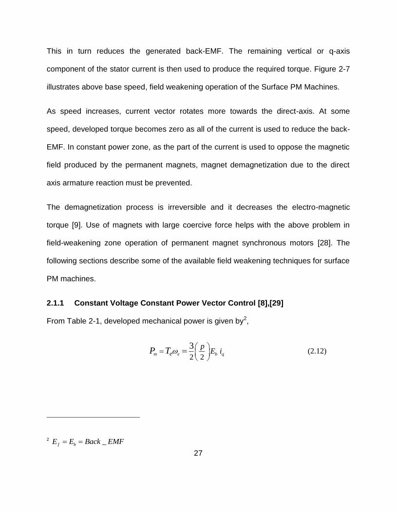
2.1.1 Constant Voltage Constant Power Vector Control [8],[29]

From Table 2-1, developed mechanical power is given by2,

2 2

3m e b qe

pE iP T

(2.12)

2 _f bE E Back EMF

28

*( )q qi L

*( )d di L

phaseV

phaseI

qI

dI

*b magE

agap

mag

*( )phaseI L

d- axis

q- axis

d di X

d di L

q qi L

Figure 2-7: Above Base Speed Operation of Surface PM Machines [8][9].

29

Therefore, in the field-weakening zone, to keep power constant, the q-axis component

of the stator current has to be changed with increase in speed.

At and above base speed b , rated power can be developed using rated value of stator

current, i.e,

From Equation(2.12),

2 2

3rated mag rated b rated b

pI KIP

(2.13)

Therefore, from Equation (2.12) and Equation (2.13) , the q-axis component of the

stator current can be derived as,

bq rated

e

i I

(2.14)

From Equation (2.5), the d-axis component of the applied stator voltage is,

* bd e q q e q rated b q rated

e

V L i L I L I

(2.15)

Note that, in constant power region, this value is constant. In this zone, as the applied

voltage is at its rated value, to keep the voltage constant, we have,

2 2

max

2 2

max

,s d q

q s d

V V V

V V V

(2.16)

30

Note that the q-axis component of the applied stator voltage is also constant. From

Equation(2.6),

2 2

max

2 2

max

,q e d d f s d

s d f

d

e d

V L i E V V

V V Ei

L

(2.17)

Note that, as speed increases, both the d-axis and q-axis components of the stator

current decrease. In this control strategy, the current vector is controlled according to

the Equation (2.14) and (2.17) to produce maximum available torque considering both

current and voltage constraints.

2.1.2 Constant Current Constant Power Vector Control [19] [30]

In this control strategy, instead of applied voltage, in the field weakening zone, applied

current is held constant. As explained in the previous section, Equation (2.14) implies

constant power operation in the field-weakening zone. To keep stator current constant,

2

2 2 2 bd s q s rated

e

i I i I I

(2.18)

From Equation (2.15) , constant q-axis current means, the d-axis component of applied

stator voltage will also be constant. So in this control strategy, the voltage vector moves

along the line d b q sV L I . In contrast to the previous method, here q-axis component of

the applied stator voltage decreases. Figure 2-8 illustrates constant current constant

power control strategy.

31

phaseV

phaseI

agap

mag d- axis

q- axis

A

B

A’

B’

.dV const

Figure 2-8: Constant Current Constant Power Vector Control.

32

2.1.3 Optimum Current Vector Control [9]

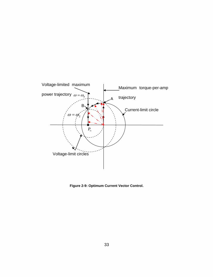
Figure 2-9 illustrates optimum current vector control strategy. Below base speed,

voltage vector is adjusted such that current will be in phase with the back-EMF

producing maximum torque-per-amp.

This can be done till point A. Point A is where current-limit circle intersects the voltage-

limit circle corresponding to the base speed. Morimoto [9] has shown that the voltage-

limited maximum power trajectory passes through the characteristics current point. So

from base speed till point B (point where current-limit circle intersects the maximum

power line), stator current can follow the current-limit circle. Note that this is not a

constant power strategy. By this control strategy maximum allowable apparent power is

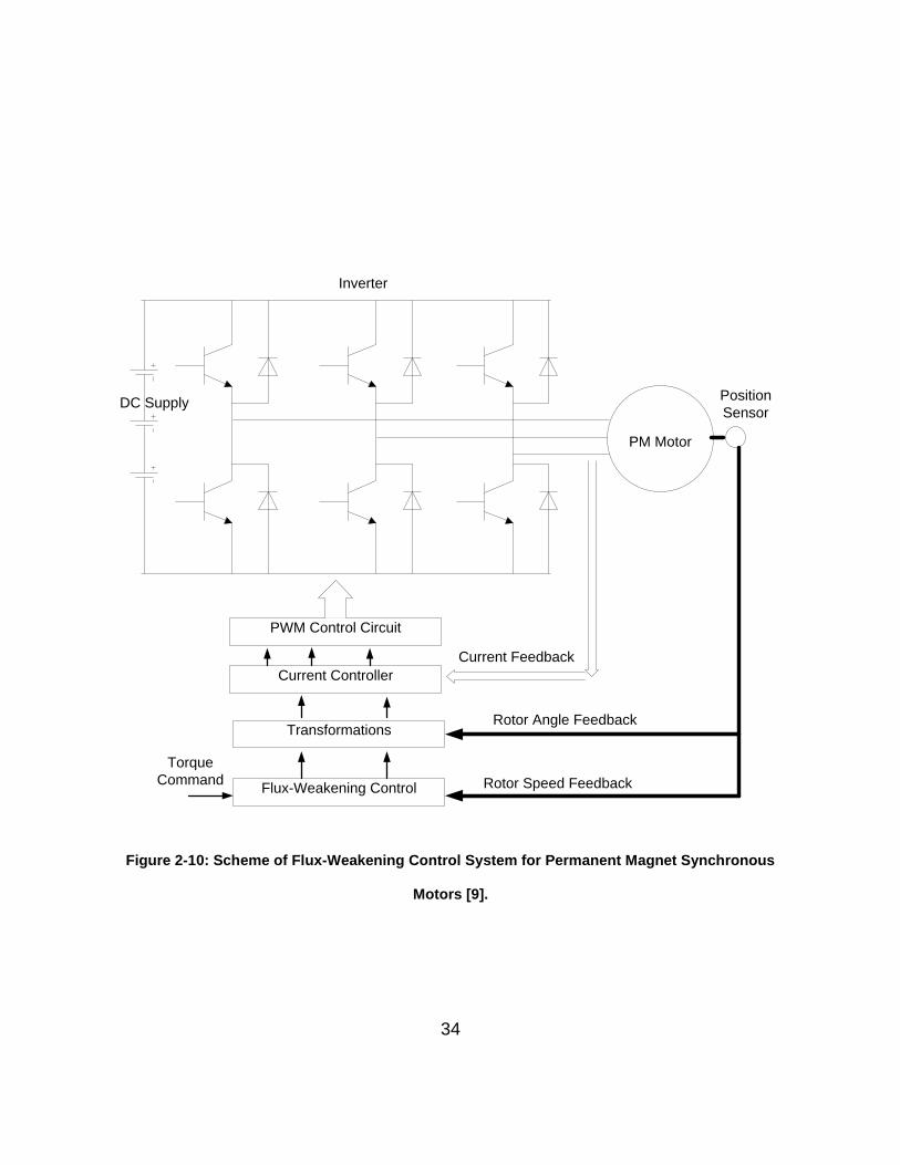
produced. Figure 2-10 illustrates this field-weakening control scheme.

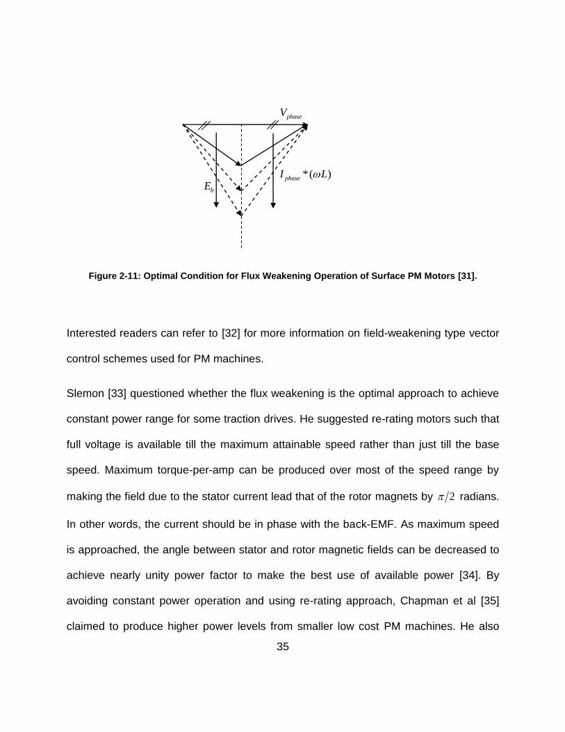
If the characteristic current of the motor is same as the rated current of the motor, i.e.

CH RatedI I , then the back-EMF ( bE ), terminal voltage ( phaseV ), and the voltage drop

across the phase inductance ( *( )phaseI L ) form an isosceles triangle. This triangle

grows at the same rate as the speed increases [31]. With this scenario, there is no

theoretical limit on the maximum speed at which the motor can be operated [31]. The

difference between the inductance voltage drop and back-EMF is what controls the

maximum attainable speed; and the closer this ratio is to unity, the higher is the

attainable speed [31]. Figure 2-11 illustrates the same. Here phaseV is the applied phase

voltage, phaseI is the resultant per phase stator current, L is the per phase winding

inductance, and bE is the generated back EMF.

33

Figure 2-9: Optimum Current Vector Control.

Voltage-limited maximum

power trajectory b

2

Current-limit circle

Voltage-limit circles

A

B

P

Maximum torque-per-amp

trajectory

34

Flux-Weakening Control

Transformations

Current Controller

PWM Control Circuit

PM Motor

Position

Sensor

Rotor Angle Feedback

Rotor Speed Feedback

Torque

Command

Inverter

DC Supply

Current Feedback

Figure 2-10: Scheme of Flux-Weakening Control System for Permanent Magnet Synchronous

Motors [9].

35

Figure 2-11: Optimal Condition for Flux Weakening Operation of Surface PM Motors [31].

Interested readers can refer to [32] for more information on field-weakening type vector

control schemes used for PM machines.

Slemon [33] questioned whether the flux weakening is the optimal approach to achieve

constant power range for some traction drives. He suggested re-rating motors such that

full voltage is available till the maximum attainable speed rather than just till the base

speed. Maximum torque-per-amp can be produced over most of the speed range by

making the field due to the stator current lead that of the rotor magnets by 2 radians.

In other words, the current should be in phase with the back-EMF. As maximum speed

is approached, the angle between stator and rotor magnetic fields can be decreased to

achieve nearly unity power factor to make the best use of available power [34]. By

avoiding constant power operation and using re-rating approach, Chapman et al [35]

claimed to produce higher power levels from smaller low cost PM machines. He also

phaseV

bE *( )phaseI L

36

outlined design choices (gear ratio, rearranging motor windings, and extending constant

volts per hertz by providing a frequency range above rated value) intended to avoid flux

weakening and improve power per unit mass ratio. Nipp [36] suggested that the

extension of speed range of PMSM is possible by connecting different coil groups of the

stator winding in different configurations. This approach requires larger motors to be

used for smaller applications increasing size, weight and cost. Otherwise it requires

extra voltage, increasing power electronics rating and hence size, cost and weight.

37

3 CONVENTIONAL PHASE ADVANCEMENT METHOD

Above base speed, the internal back-EMF exceeds maximum available supply voltage.

Thus as the speed of the motor approaches the base speed, the ability of an inverter to

force current into motor winding diminishes. This causes torque reduction and ultimately

puts limitation on the achievable maximum speed.

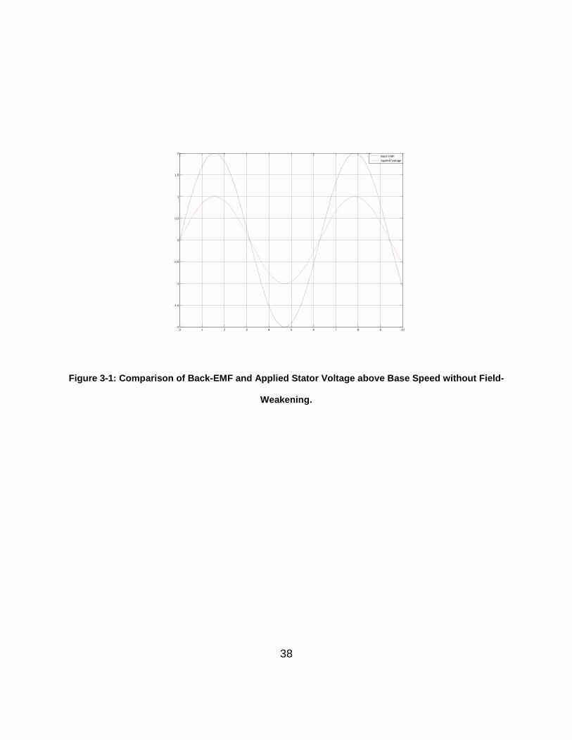
In Figure 3-1, the red curve represents applied voltage and the black curve represents

generated back-EMF. Note that back-EMF exceeds the applied voltage making it

difficult to force any current into the motor.

In vector control, as discussed in the previous chapter, above base speed, d-axis

current is applied such that it reduces the resultant air-gap magnetic field. This causes

reduction in generated back-EMF. This helps the inverter to force current into the motor

winding and develop the required torque at higher speeds. This traditional “flux

weakening” method, if not used properly, can cause irreversible demagnetization of the

rotor permanent magnets [9].

Vector control requires information about the phase currents and voltages. These three-

phase quantities have to be transformed into equivalent d-q values. Based on control,

error values (d-q) have to be transformed back to the three phase values. Based on this

information along with Pulse Width Modulation technique used, inverter switches are

turned ON or OFF.

38

Figure 3-1: Comparison of Back-EMF and Applied Stator Voltage above Base Speed without Field-

Weakening.

0 1 2 3 4 5 6 7 8 9 10-2

-1.5

-1

-0.5

0

0.5

1

1.5

2Back EMF

Applied Voltage

39

This means vector control requires precise information about the phase currents and

phase voltages. This implies more drive hardware, size and weight. An Abc-dq

transformation means more mathematical complexity, slower system response and

more required computational power. The primary goal of this research was to reduce

this mathematical complexity. This can be done by avoiding vector control type field

weakening scheme which also reduces the need for voltage and current sensors.

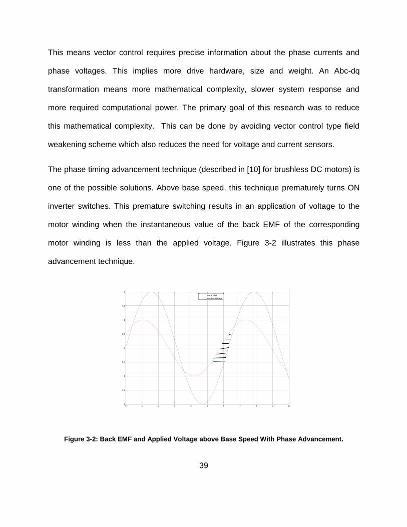
The phase timing advancement technique (described in [10] for brushless DC motors) is

one of the possible solutions. Above base speed, this technique prematurely turns ON

inverter switches. This premature switching results in an application of voltage to the

motor winding when the instantaneous value of the back EMF of the corresponding

motor winding is less than the applied voltage. Figure 3-2 illustrates this phase

advancement technique.

Figure 3-2: Back EMF and Applied Voltage above Base Speed With Phase Advancement.

0 1 2 3 4 5 6 7 8 9 10-2

-1.5

-1

-0.5

0

0.5

1

1.5

2

Back EMF

Applied Voltage

40

Phase timing advancement results in “pre-charging” of the winding with current. By the

time the rotor rotates to a position where generated back-EMF exceeds applied

voltage, current in the winding has already been raised to a level that can produce

significant torque even though the same current starts decreasing due to the negative

relative voltage applied across the motor inductance. This results in significant increase

in maximum motor speed at which constant power can be developed.

3.1 Analysis of a Permanent Magnet Synchronous Motor Driven by

Conventional Phase Timing Advancement Method [37].

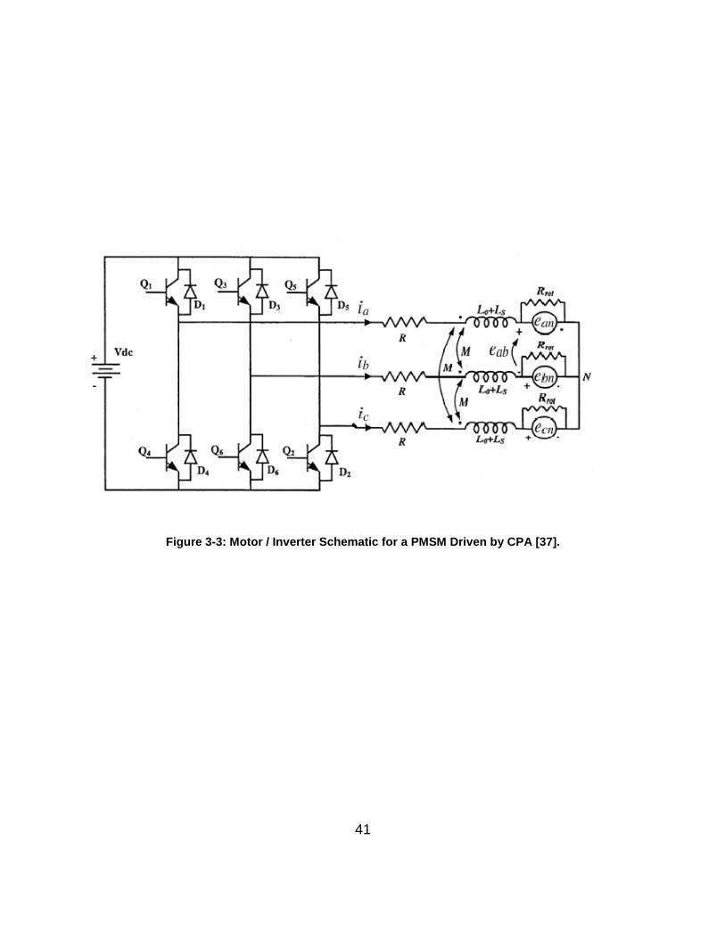
Figure 3-3 shows a schematic of a three-phase PMSM driven by a voltage-source

inverter (VSI). Figure 3-3 also defines some of the parameters and notations used in

this discussion. Here p = number of poles, N=actual mechanical rotor speed in

revolutions per minute (rpm), Nb = mechanical base speed in rpm, n = relative

speed = ,bN

N b = base speed in electrical radians/sec, = *2 *

2 60

bNp

, = actual rotor

speed in electrical radians/sec, = nb, Eb = rms magnitude of the phase-to-neutral emf

at base speed, IR = rated rms motor current, PR = rated output power = 3EbIR, Ls =self

inductance per phase, Lo = leakage inductance per phase, M = mutual

inductance, L = equivalent inductance per phase = Lo + Ls + M, R = winding resistance

per phase, van=applied phase A to neutral voltage, ean = phase A to neutral back-

EMF and, eab = phase A to phase B (line-to-line) back-EMF.

41

Figure 3-3: Motor / Inverter Schematic for a PMSM Driven by CPA [37].

42

First part of the Figure 3-3, is a typical voltage source inverter configuration. Here DC

supply voltage is denoted by Vdc. Typically a battery is used as a DC supply source. Q1,

Q2, Q3, Q4, Q5, and Q6 are solid state power electronics switches. Typically IGBTs are

used as inverter switches. Similarly D1, D2, D3, D4, D5, and D6 are bypass diodes.

Switches in an inverter of Figure 3-3, can be controlled by a well known method called

as sinusoidal pulse width modulation (SPWM) technique. This inverter switching

scheme uses a triangular carrier wave (green color waveform shown in Figure 3-4, Vtri)

and three sinusoidal reference waveforms (shown in blue for phase A , yellow for

phase B and, red for phase C, i.e. Vcontrol ) to decide the switching pattern. For phase A,

if control triV V , upper switch Q1 is turned ON , similarly when control triV V , lower switch Q4

is turned ON.

Figure 3-4: Three Phase Waveforms.

Time

0s 1.0ms 2.0ms 3.0ms 4.0ms 5.0ms 6.0ms 7.0ms 8.0ms 9.0ms

v(27,0) v(28,0) v(29,0) v(30,0)

-1.0V

-0.5V

0V

0.5V

1.0V

43

Simultaneous switching of both of these switches in one inverter leg will result in short

circuit of a DC supply. As it takes a small but finite time for switches to change the state,

to avoid short circuit usually a dead time is inserted between changes of state. The

amplitude and frequency of an inverter output waveform (applied stator voltage) is

determined by the amplitude and frequency of the controlV waveform. This frequency is

called the fundamental frequency. Usually the amplitude of the triangular waveform is

kept at unity and the amplitude of a sinusoidal control waveform is changed. The ratio of

/control triV V is called the modulation index am . When the modulation index am is more

than 1, the inverter is said to be operating in an over-modulation region and the

switching waveform looks like a square wave. Maximum value of the am is 4 / . The

frequency of Vtri waveform is called the switching frequency. The switching frequency is

usually in KHz to obtain a sinusoidal shape in the resultant stator current.

The remaining part of Figure 3-3 is a typical PMSM motor model. Resistors R and Rrot,

represent the copper losses and the speed sensitive rotational losses of a typical PMSM

motor respectively. The value of Rrot can be calculated for any given speed using the

least-squares fit of a back-EMF data and the least squares-fit of rotational no-load

losses data. At relative speed n, the value of (n) is calculated as,

23 b

rot

rot

nER n

P n (3.1)

.

rotR

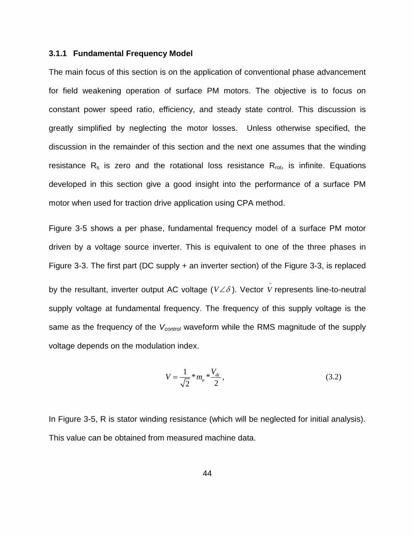
44

3.1.1 Fundamental Frequency Model

The main focus of this section is on the application of conventional phase advancement

for field weakening operation of surface PM motors. The objective is to focus on

constant power speed ratio, efficiency, and steady state control. This discussion is

greatly simplified by neglecting the motor losses. Unless otherwise specified, the

discussion in the remainder of this section and the next one assumes that the winding

resistance Rs is zero and the rotational loss resistance Rrot, is infinite. Equations

developed in this section give a good insight into the performance of a surface PM

motor when used for traction drive application using CPA method.

Figure 3-5 shows a per phase, fundamental frequency model of a surface PM motor

driven by a voltage source inverter. This is equivalent to one of the three phases in

Figure 3-3. The first part (DC supply + an inverter section) of the Figure 3-3, is replaced

by the resultant, inverter output AC voltage (V ). Vector ~

V represents line-to-neutral

supply voltage at fundamental frequency. The frequency of this supply voltage is the

same as the frequency of the Vcontrol waveform while the RMS magnitude of the supply

voltage depends on the modulation index.

1

* * ,22

dca

VV m (3.2)

In Figure 3-5, R is stator winding resistance (which will be neglected for initial analysis).

This value can be obtained from measured machine data.

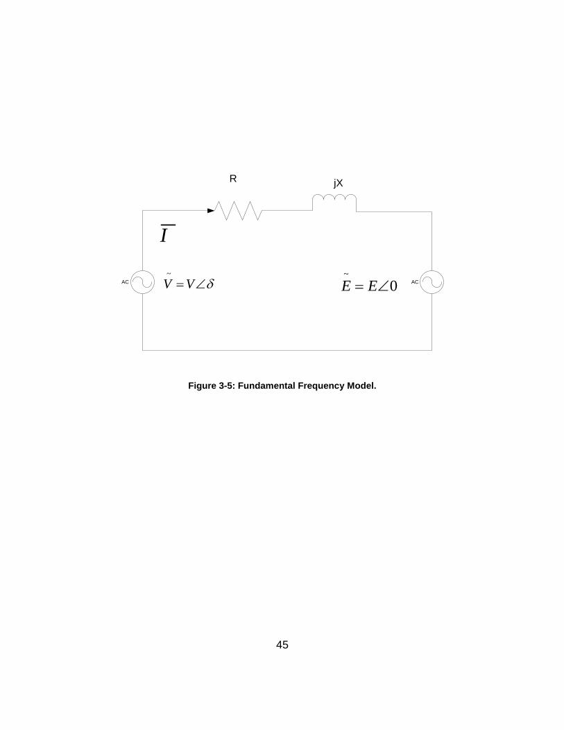
45

AC AC

~

V V ~

0E E

R jX

I

Figure 3-5: Fundamental Frequency Model.

46

Similarly, the motor per phase winding reactance can be expressed as,

b

b

b

X L

X L

X nX

(3.3)

Value of per-phase stator winding inductance (L) can also be obtained from the

measured machine data. Here is the per-phase winding reactance at base speed

and n is the relative speed of the motor compared to the base speed. Vector ~

E

represents the phase-to-neutral generated motor back-EMF. This vector is chosen as a

reference vector. Its phase angle will always be zero. Magnitude of this back-EMF is

linear in motor speed. The voltage constant Kv, has units of RMS volts per electrical

radian per second. Thus, the RMS value of the back-EMF at any motor speed is given

by,

v

b v

b

b

E K

E K

E nE

(3.4)

Here is the RMS magnitude of line-to-neutral back-EMF at base speed and n is the

relative motor speed compared to the base speed. A detailed PSPICE simulator was

developed to analyze the performance of a PM synchronous motor, controlled by PWM

when operating at a constant speed, based on the fundamental frequency model. This

bX

bE

47

model of the motor drive is applicable at a selectable but constant speed. As the motor

speed increases, generated back-EMF increases. Supply voltage has to be increased

proportionally. Based on the available DC supply voltage, base speed nb, can be

defined as the highest speed at which applied voltage will be at its rated value. At this

point, modulation index 4 /am and 2 * dcV V . The base speed is also the highest

speed at which rated torque is required, and can be produced. Power developed at this

point is the rated power. True base speed nbt , is exactly same as the actual base

speed when the dc supply voltage is the minimum value that permits rated torque to be

developed at the base speed. For sinusoidal PWM, we have,

1

* * ,22

dcout a

VV m (3.5)

From Figure 3-5, we have,

*( ) ( )b bV I R jnX nE (3.6)

Assume that the rated current is in phase with back-EMF to produce maximum torque-

per-amp.

Neglecting resistance, at base speed (n = 1), with modulation index at 4 , we have,

22

_ min2

dc b b rV E X I

(3.7)

48

Here rI is the rated RMS stator winding current. Note that Equation (3.7) insures that

sufficient dc supply voltage is provided so that at base speed, the driving voltage is

sufficient not only to overcome the back-EMF voltage but also internal impedance of the

motor. If the DC supply voltage is less than Vdc_min , it will not be possible to develop the

rated torque at the specified base speed and the true base speed will be less than the

specified value. If the DC supply voltage is larger than Vdc_min , then the true base

speed will be greater than the specified value. Letting the true base speed be denoted

as nbt we have,

min

dcbt b

dc

Vn n

V

(3.8)

When the DC supply is larger than the minimum, the rated torque can be developed at a

speed higher than the base speed resulting in greater power conversion capability.

However, the drive control can be configured to preclude this extra capability restricting

the maximum power above base speed to the rated power. Even though control may

be used to constrain the torque speed envelope, the addition of surplus dc supply

voltage may allow reduced current magnitude at higher speeds, thereby reducing

inverter and motor copper losses and improving efficiency. This possibility is discussed

further.

3.1.2 Below Base Speed Operation (Constant Torque Zone, n≤1)

In the constant torque zone, both the magnitude of the applied stator voltage V, and the

angle can be adjusted. This allows motor current to be in phase with the back-EMF.

49

From Figure 3-5, voltage magnitude V, and inverter lead angle can be calculated as

follows;

2 2 1

22 1

tan

tan

b b

bb b

b

bb b

b

V nE jnIX

nIXnE nIX

nE

IXn E X I

E

V

. (3.9)

Note that inverter lead angle does not depend on the speed. It only depends on the

current required to produce desired torque. It also depends on motor design parameters

at base speed such as phase reactance and back-EMF.

Equation (3.9) applied to Figure 3-5, neglecting resistance, we have RMS current,

~ cos0 sin bb

b b b

nE VV nE VI j

jnX nX nX

(3.10)

As speed increases, the modulation index has to be increased from 0 to 4/ so that the

applied voltage overcomes back-EMF and the winding reactance voltage drop. From

Equation (3.9), it can be seen that, for the constant current, the applied voltage vector

extends from the origin at constantuntil it reaches its maximum value. Assuming that

the DC supply voltage is minimum given by Equation (3.7), modulation index is 4/

and stator current is the rated current, maximum phase voltage magnitude can be

calculated as,

50

22

max b b rV E X I (3.11)

Similarly, inverter lead angle is given by,

1tan r b

b

I X

E

(3.12)

With the rated current, the power developed at the base speed will be the rated power.

Since the current is in phase with the back-EMF, for 3-phase rated power Pr, we have,

3r b rP E I (3.13)

At base speed, the constant torque region ends. If applied DC voltage is more than (3.7)

, the true base speed will be more than the designed base speed. Although control can

be used such that applied voltage is limited to the designed base speed value. Above

base speed starts constant power region.

3.1.3 Operation above Base Speed (Constant Power Region, n≥1)

Above base speed voltage magnitude maxV V i.e. sinusoidal PMW is operating in the

over-modulation region. Neglecting the armature resistance, from Figure 3-5, current

vector is given by,

max maxsin cos ,b

b b b

r x

V E VI j

nX X nX

I I jI

(3.14)

51

It can be seen from Equation (3.14) that this stator current has two parts a) Real part –

which is responsible for mechanical torque production, and b) Imaginary part.

Here is the component of motor current which is in phase with the back-EMF. This

component is like a q-axis current component in the d-q model and it can be referred to

as a torque producing current component. is the component of a phase current that is

orthogonal to the back-EMF and results in no net torque production. This component is

like a d-axis component of the current in the d-q model and can be referred to as a field

weakening current. Total motor current has RMS magnitude,

2 2

2 2 2

max max

,

2 cos

r x

b b

b

I I I

V n V E n EI

nX

(3.15)

From Figure 3-5, the apparent inverter output power (or motor input power) can be

derived as follows,

*

*

maxmax

* ,

0( )*

in

bin

b

S V I

V nES V

jnX

(3.16)

Therefore motor input power is given by,

*

max

3Re( ),

3 sin

in

bin

b

P VI

V EP

X

(3.17)

rI

xI

52

Similarly, total motor output power is given by,

*

max

3Re( ),

3 sin

m

bm

b

P EI

V EP

X

(3.18)

and

maxmax 3 b

b

V EP

X (3.19)

Here Pmax, is the maximum power that can possibly be converted to mechanical form.

This power corresponds to the lead angle being 90. From Equation (3.17) and

Equation (3.18), it can be seen that, motor output power is equal to the motor input

power. As we have neglected the winding resistance, efficiency is 100%. Since the

losses are zero, all the power from first part of the Figure 3-5 is transferred to the

second part of the figure. Common value of this power is,

max3 sinbm in

b

V EP P

X (3.20)

This expression shows that, it is easy to control surface PM motor to deliver rated power

in constant power zone. Inverter lead angle , has to be held fixed at a value that

causes motor output power in Equation (3.20) to be equal to the rated power of the

motor given by Equation (3.13).We have,

1

max

sin3

b r

b

X P

V E

(3.21)

53

While constant lead angle control allows the PMSM to operate at a constant power

above base speed, it is not a certainty that doing so results in operation within the rated

motor current limit. The critical factor is the motor inductance as shown in the next

section.

3.1.4 “Optimal” Inductance for the Field-Weakening

Observe from Equations (3.14) that as the speed approaches infinity, motor current

magnitude approaches a limiting value given by,

max max

max

max

lim lim sin cos ,

lim lim sin 0

lim lim cos

b

n nb b b

rn n

b

b b bx

n nb b b b

V E VI j

nX X nX

VI

nX

E V E EI

X nX X L

(3.22)

Equation (3.15) gives the value of RMS motor current, when operating at any speed

above base speed. Equation (3.21) gives the value of the lead angle such that the

rated power is produced in the constant torque zone. In order to keep the current

required to produce this rated power below the rated current value , we have ,

2 2 2

max max

2 2

max

2 cos

2,

b b

b

b

b

r

V nV E n EI

nX

V n n EI

n L

I I

(3.23)

RI

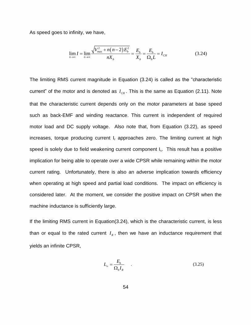
54

As speed goes to infinity, we have,

2 2

max 2lim lim

b b bCH

n nb b b

V n n E E EI I

nX X L

(3.24)

The limiting RMS current magnitude in Equation (3.24) is called as the “characteristic

current” of the motor and is denoted as . This is the same as Equation (2.11). Note

that the characteristic current depends only on the motor parameters at base speed

such as back-EMF and winding reactance. This current is independent of required

motor load and DC supply voltage. Also note that, from Equation (3.22), as speed

increases, torque producing current Ir approaches zero. The limiting current at high

speed is solely due to field weakening current component Ix. This result has a positive

implication for being able to operate over a wide CPSR while remaining within the motor

current rating. Unfortunately, there is also an adverse implication towards efficiency

when operating at high speed and partial load conditions. The impact on efficiency is

considered later. At the moment, we consider the positive impact on CPSR when the

machine inductance is sufficiently large.

If the limiting RMS current in Equation(3.24), which is the characteristic current, is less

than or equal to the rated current , then we have an inductance requirement that

yields an infinite CPSR,

. (3.25)

CHI

RI

b

b R

EL

I

55

This inductance value is sometimes cited as the “optimal” value for field weakening [27],

[31], [8]. Theoretically, any surface permanent magnet synchronous machine having an

inductance value equal to Equation (3.25) or higher, will have an infinite CPSR.

In the constant power region, there is a well defined speed at which current magnitude

is minimal. Setting the derivative of Equation (3.15) with respect to relative speed n,

equal to zero and solving for this speed yields,

maxmin

cosb

Vn

E . (3.26)

.

With this value of substituted into Equation (3.15), the minimum current can found.

min

max3

PI

V (3.27)

Note that this minimum current magnitude is independent of motor parameters and

depends linearly on the developed power and inversely on the maximum fundamental

frequency component of the inverter output voltage. Since can be increased by

raising the dc supply voltage, there may be a reduction in motor and inverter losses

when is increased above the minimum level required to sustain rated power at base

speed. It can be shown that for speeds less than nmin , the inverter power factor is

lagging; while for speeds above nmin , the inverter power factor is leading. Thus, the

inverter operates at the optimum unity power factor condition at only one speed, namely

n

maxV

dcV

56

nmin. Figure 3-6 illustrates this conventional phase advancement control strategy when

used for the flux weakening of surface permanent magnet synchronous machines.

In this figure, red vector represents the stator current. Up to base speed, the current is

maintained in phase with the back-EMF. This produces the maximum torque per amp.

Simulation and the experimental results (as described later) suggest that, from base

speed till nmin, stator current decreases with increase in speed to the minimum value. At

this speed, current is phase with the applied voltage. So power factor is unity. Below

this speed, the power factor is lagging. Above nmin, the current increases with speed and

approaches the characteristic current. If this characteristic current is less than the rated

current of the motor, theoretically surface PM machines have infinite CPSR. Above nmin,

the power factor is leading as the back-EMF exceeds the rated supply voltage.

3.2 Steady State PMSM Control Considering Winding Resistance

The mathematical analysis given in previous section neglected winding resistance.

Neglecting these factors makes the analysis simpler. It leads to compact expressions

which provide considerable insight into the control of surface PM motors for traction

drive application, using conventional phase advancement method. Stator current can be

considered as a control variable. Depending on the load (torque/power) requirement,

the required motor current can be estimated. This required motor current can be

achieved by controlling the magnitude and the angle of applied stator voltage.

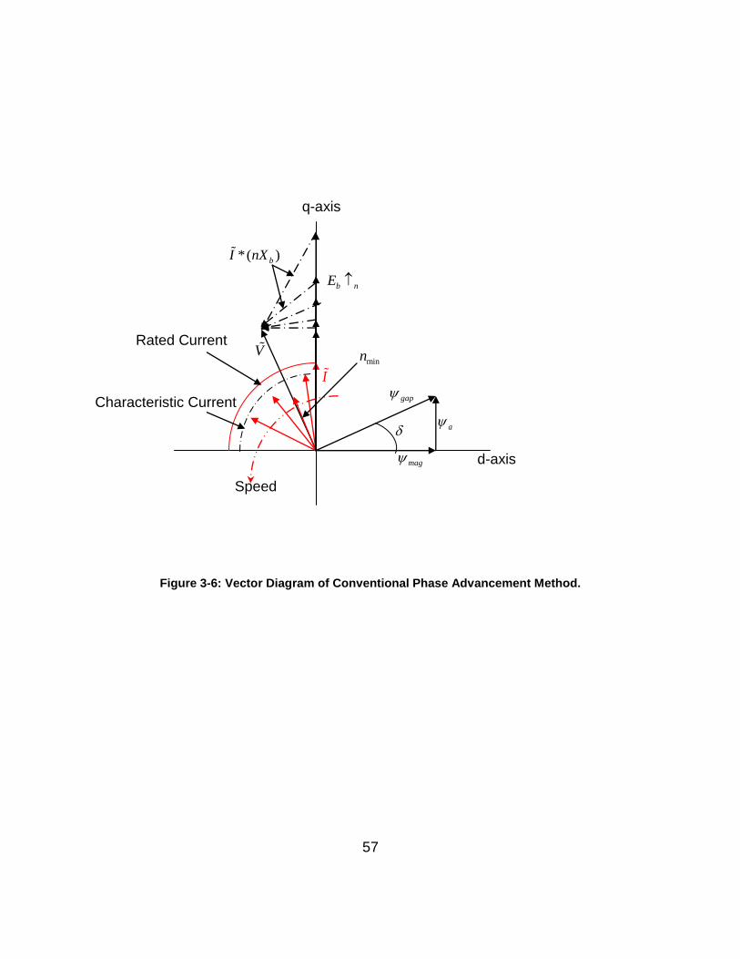
57

Figure 3-6: Vector Diagram of Conventional Phase Advancement Method.

d-axis mag

gap

a

b nE

V

I

Speed

Rated Current

Current

minn

*( )bI nX

q-axis

Characteristic Current

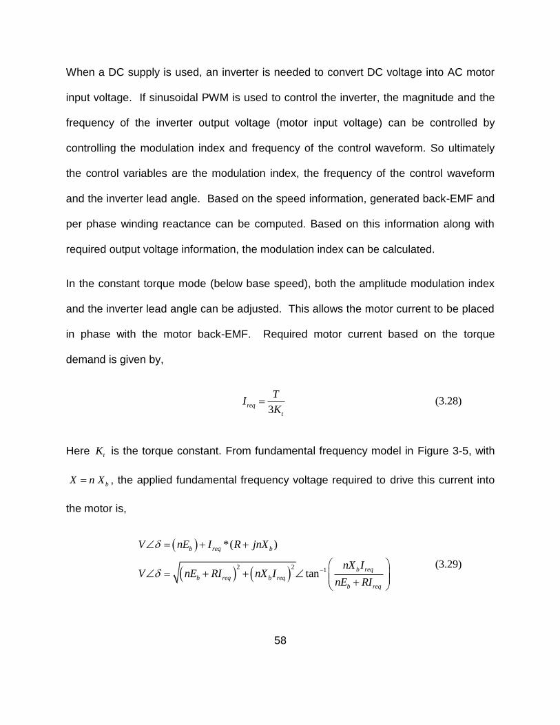
58

When a DC supply is used, an inverter is needed to convert DC voltage into AC motor

input voltage. If sinusoidal PWM is used to control the inverter, the magnitude and the

frequency of the inverter output voltage (motor input voltage) can be controlled by

controlling the modulation index and frequency of the control waveform. So ultimately

the control variables are the modulation index, the frequency of the control waveform

and the inverter lead angle. Based on the speed information, generated back-EMF and

per phase winding reactance can be computed. Based on this information along with

required output voltage information, the modulation index can be calculated.

In the constant torque mode (below base speed), both the amplitude modulation index

and the inverter lead angle can be adjusted. This allows the motor current to be placed

in phase with the motor back-EMF. Required motor current based on the torque

demand is given by,

3

req

t

TI

K (3.28)

Here tK is the torque constant. From fundamental frequency model in Figure 3-5, with

, the applied fundamental frequency voltage required to drive this current into

the motor is,

2 2

1

*( )

tan

b req b

b req

b req b req

b req

V nE I R jnX

nX IV nE RI nX I

nE RI

(3.29)

bX n X

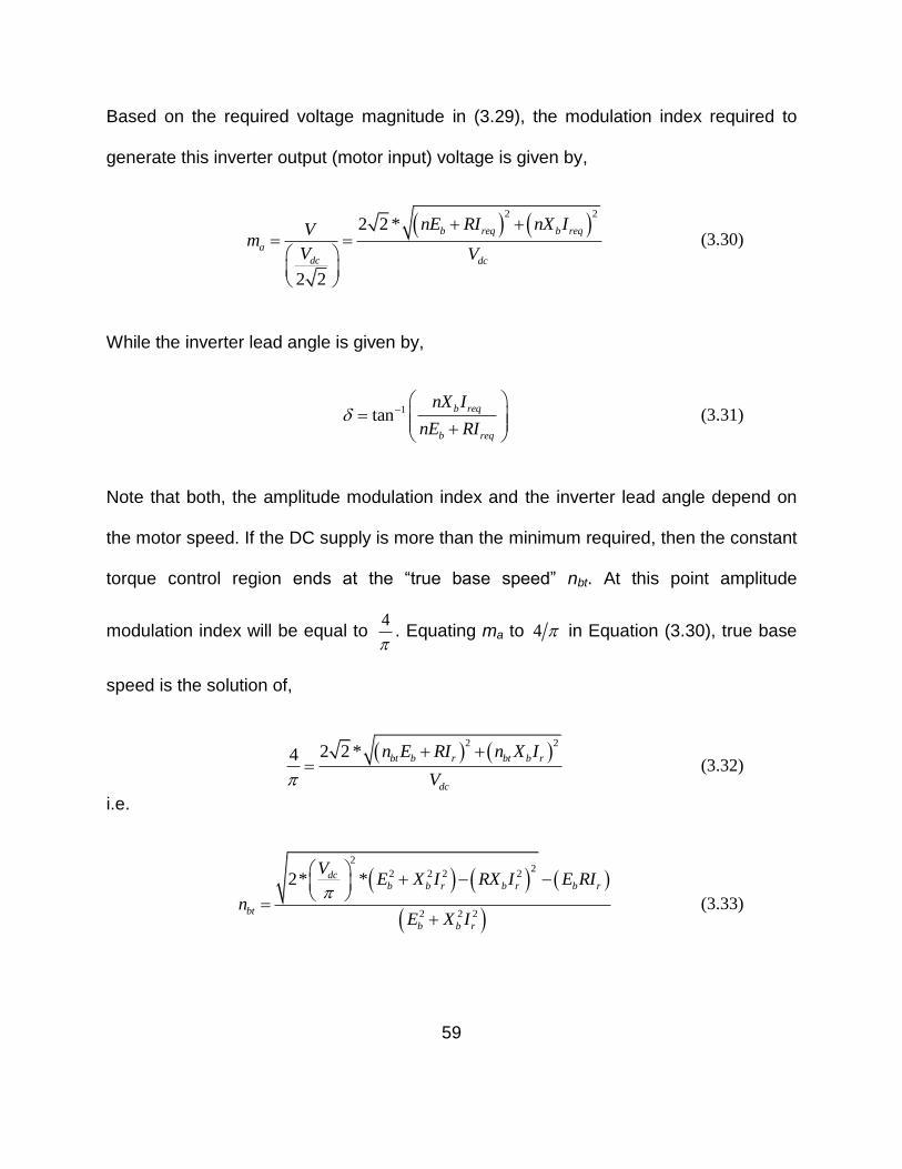
59

Based on the required voltage magnitude in (3.29), the modulation index required to

generate this inverter output (motor input) voltage is given by,

2 2

2 2 *

2 2

b req b req

a

dc dc

nE RI nX IVm

V V

(3.30)

While the inverter lead angle is given by,

1tanb req

b req

nX I

nE RI

(3.31)

Note that both, the amplitude modulation index and the inverter lead angle depend on

the motor speed. If the DC supply is more than the minimum required, then the constant

torque control region ends at the “true base speed” nbt. At this point amplitude

modulation index will be equal to . Equating ma to 4 in Equation (3.30), true base

speed is the solution of,

2 22 2 *4 bt b r bt b r

dc

n E RI n X I

V

(3.32)

i.e.

22

2 2 2 2

2 2 2

2* *dcb b r b r b r

bt

b b r

VE X I RX I E RI

nE X I

(3.33)

4

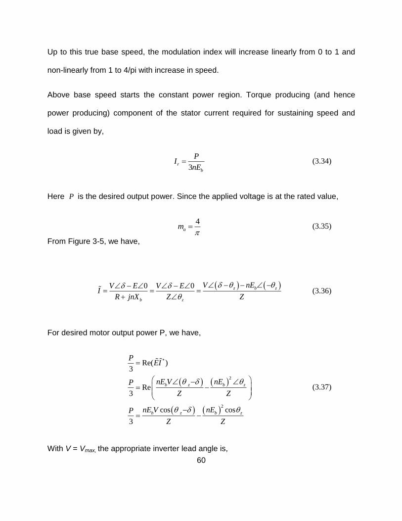
60

Up to this true base speed, the modulation index will increase linearly from 0 to 1 and

non-linearly from 1 to 4/pi with increase in speed.

Above base speed starts the constant power region. Torque producing (and hence

power producing) component of the stator current required for sustaining speed and

load is given by,

3

r

b

PI

nE (3.34)

Here is the desired output power. Since the applied voltage is at the rated value,

4

am

(3.35)

From Figure 3-5, we have,

0 0 z b z

b z

V nEV E V EI

R jnX Z Z

(3.36)

For desired motor output power P, we have,

*

2

2

Re( )3

Re3

cos cos

3

b z b z

b z b z

PEI

nE V nEP

Z Z

nE V nEP

Z Z

(3.37)

With V = Vmax, the appropriate inverter lead angle is,

P

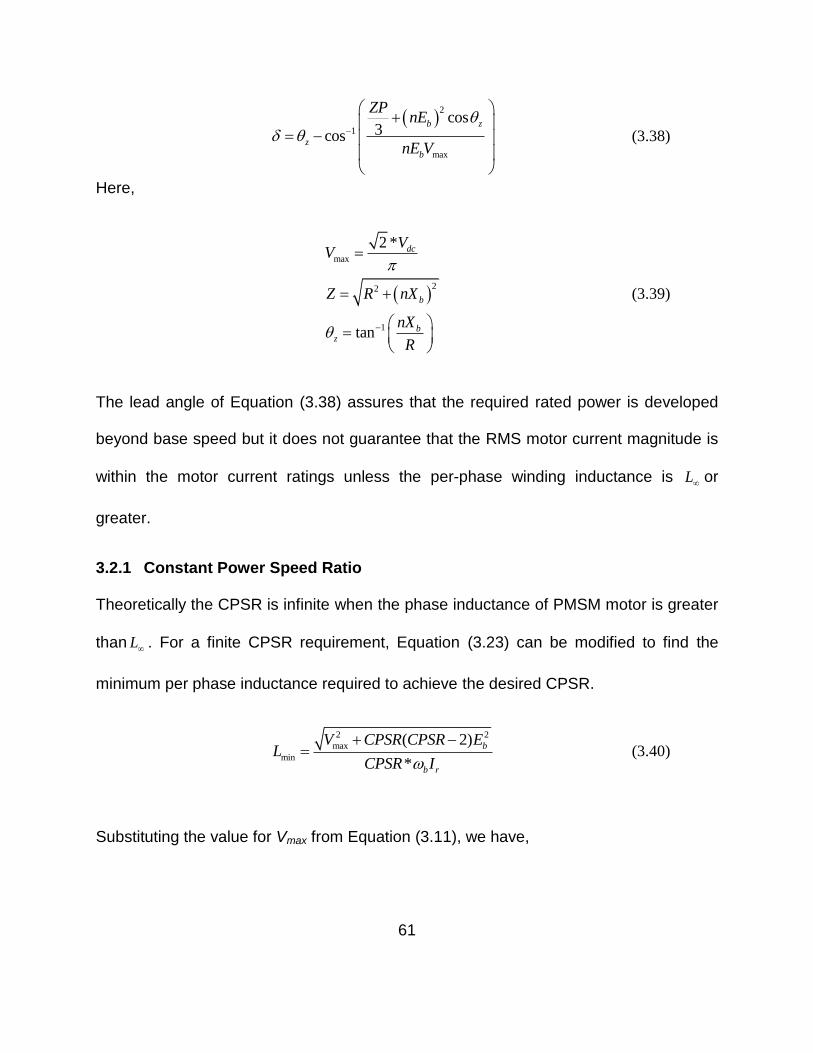
61

2

1

max

cos3cos

b z

z

b

ZPnE

nE V

(3.38)

Here,

max

22

1

2 *

tan

dc

b

bz

VV

Z R nX

nX

R

(3.39)

The lead angle of Equation (3.38) assures that the required rated power is developed

beyond base speed but it does not guarantee that the RMS motor current magnitude is

within the motor current ratings unless the per-phase winding inductance is or

greater.

3.2.1 Constant Power Speed Ratio

Theoretically the CPSR is infinite when the phase inductance of PMSM motor is greater

than L . For a finite CPSR requirement, Equation (3.23) can be modified to find the

minimum per phase inductance required to achieve the desired CPSR.

2 2

max

min

( 2)

*

b

b r

V CPSR CPSR EL

CPSR I

(3.40)

Substituting the value for Vmax from Equation (3.11), we have,

L

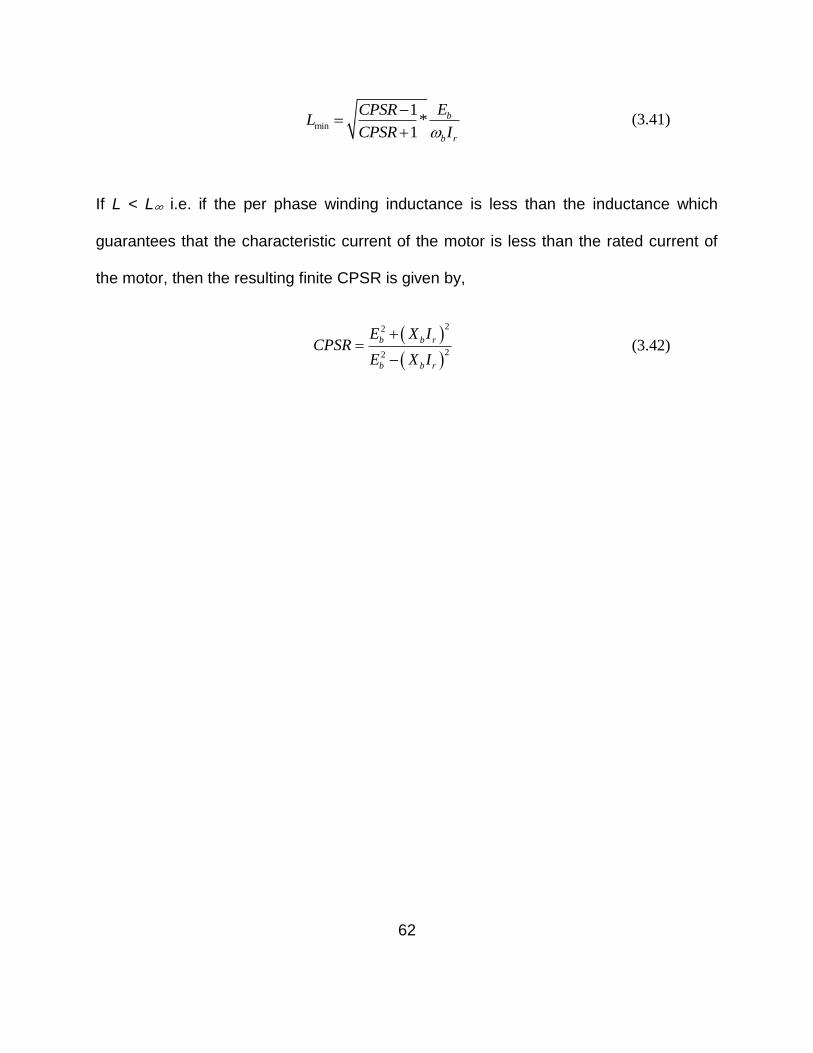
62

min

1*

1

b

b r

ECPSRL

CPSR I

(3.41)

If L < L∞ i.e. if the per phase winding inductance is less than the inductance which

guarantees that the characteristic current of the motor is less than the rated current of

the motor, then the resulting finite CPSR is given by,

22

22

b b r

b b r

E X ICPSR

E X I

(3.42)

63

4 SIMULATIONS and EXPERIMENTAL VERIFICATION of CONVENTIONAL PHASE ADVANCEMENT METHOD FOR SURFACE PM MACHINES.

A 30-pole, 6-kW, and 6000 rpm prototype of a permanent magnet synchronous motor

(PMSM) with fractional-slot concentrated-windings was designed and developed by the

University of Wisconsin, Madison [27]. Compared to the regular PMSMs with distributed

winding, this machine has significantly more inductance [27], making it an ideal

candidate for field weakening type control scheme. In April 2006, this prototype was

delivered to the Oak Ridge National Laboratory (ORNL) for testing the CPA based

controller. The control scheme based on conventional phase timing advancement is

very simple compared to the vector control based field weakening scheme. It is low-cost

because this control method does not require current or phase voltage sensors.

The following table shows parameters of the surface permanent magnet motor with

factional-slot concentrated windings used for simulation and experimental verification

purpose.

4.1 Simulink Based Simulation Model

Figure 4-1 shows the algorithm for simulating a CPA based PSMS drive. This model

assumes that the motor parameters, which includes per phase inductance, resistance,

and back-EMF are known.

64

Table 4-1: Parameters of a Surface Permanent Magnet Synchronous Motor with Fractional-Slot

Concentrated Windings.

Parameter Measured value

Number of Poles, p 30

Base Speed, Nb 900 RPM

Back-EMF at Base Speed, Eb 49.45

Voltage Constant, KV 0.03497

Rated Power, Pr 6 kW

Rated Torque, Tr 63.66 Nm

Rated RMS Current, Ir 40.44 A

Per Phase Winding Resistance, R 76 mΩ

Per Phase Inductance, L 1.3 mH

65

Figure 4-1: Simulink Model for CPA driven PMSM Simulation.

ncom

900

Vehicle Dynamics

Te

thetae

spd

we

pe

Stator Voltage

Stator Current

Speed

Saturation 1

SaturationProportional Gain

k

PWM/Inverter

Ma

del

V1

PWM Logic

icom

we

Ma

del

Motor Model

V1

we

I1

theta1

Te

Modulation Index

Integrator

1

s

Gain 2

-K-

Gain 1

-K-

Error - Current Command

DeltaComplex to

Magnitude -Angle

|u|

u

66

Here ncom is the speed command. Speed error is generated by comparing ncom with

speed feedback from the vehicle dynamics block. This error, processed through a PI

controller, is used as the stator current command. Based on this current requirement,

required stator voltage magnitude and angle is calculated by using Equation (3.29).

Based on the speed feedback, current command, and region of operation (constant

torque or constant power), PWM Logic block calculates the modulation index and

inverter lead angle by using Equations (3.28), (3.30), and (3.31) or Equations (3.34),

(3.35). PWM / Inverter block represents the inverter model. Magnitude of the generated

voltage is nothing but *2 2

DCVMa and is the angle of this motor input voltage. Motor

Model block, based on the information about applied voltage, along with the information

about per-phase inductance, resistance and back-EMF, estimates the resultant stator

current by using Equation (3.36). Based on this stator current, output torque is

calculated using the Equation (3.13).

This output torque is then compared with the load torque information obtained from the

road load equations. Following differential equation describes the Vehicle Dynamics

block. We have,

.

m m e lJ D T T (4.1)

Here J is the motor inertia constant; D is the damping constant, eT is the electrical

torque generated by the motor, lT is the load torque (also called as a road load) and m

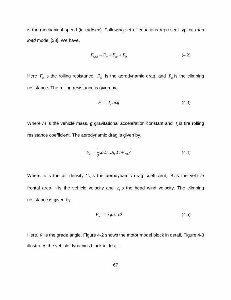
67

is the mechanical speed (in rad/sec). Following set of equations represent typical road

load model [38]. We have,

total rr ad crF F F F (4.2)

Here rrF is the rolling resistance, adF is the aerodynamic drag, and crF is the climbing

resistance. The rolling resistance is given by,

. .rr rF f m g (4.3)

Where m is the vehicle mass, g gravitational acceleration constant and rf is tire rolling

resistance coefficient. The aerodynamic drag is given by,

2

0

1. . . .( )

2ad D fF C A v v (4.4)

Where is the air density, DC is the aerodynamic drag coefficient, fA is the vehicle

frontal area, v is the vehicle velocity and 0v is the head wind velocity. The climbing

resistance is given by,

. .sincrF m g (4.5)

Here, is the grade angle. Figure 4-2 shows the motor model block in detail. Figure 4-3

illustrates the vehicle dynamics block in detail.

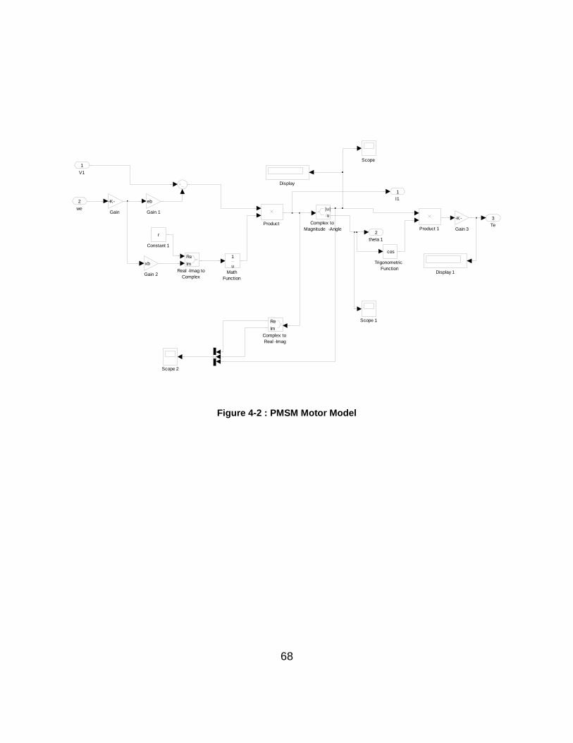
68

Figure 4-2 : PMSM Motor Model

Te

3

theta 1

2

I1

1

Trigonometric

Function

cos

Scope 2

Scope 1

Scope

Real -Imag to

Complex

Re

Im

Product 1Product

Math

Function

1

u

Gain 3

-K-

Gain 2

xb

Gain 1

eb

Gain

-K-

Display 1

Display

Constant 1

r

Complex to

Real -Imag

Re

Im

Complex to

Magnitude -Angle

|u|

u

we

2

V1

1

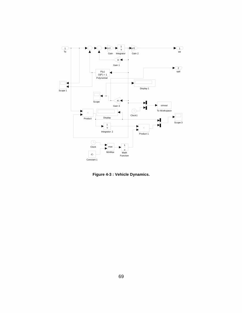
69

Figure 4-3 : Vehicle Dynamics.

spd

2

we

1

To Workspace

simout

Scope 3

Scope 1

Scope

Product 1

Product

Polynomial

P(u)

O(P) = 1

MinMax

max

Math

Function

1

u

Integrator 2

1

s

Integrator

1

s

Gain 3

-K-

Gain 2

p/2

Gain 1

D

Gain

1/J

Display 1

Display

Constant 1

-C-

Clock1

Clock

Te

1

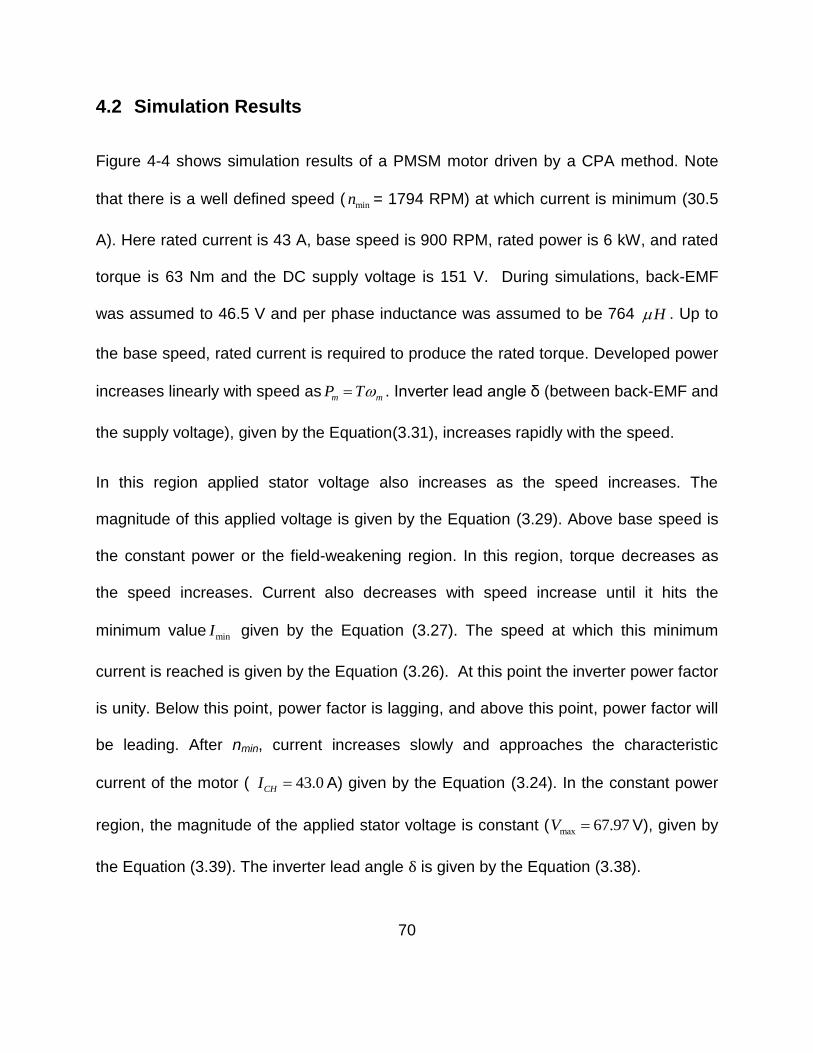
70

4.2 Simulation Results

Figure 4-4 shows simulation results of a PMSM motor driven by a CPA method. Note

that there is a well defined speed ( minn = 1794 RPM) at which current is minimum (30.5

A). Here rated current is 43 A, base speed is 900 RPM, rated power is 6 kW, and rated

torque is 63 Nm and the DC supply voltage is 151 V. During simulations, back-EMF

was assumed to 46.5 V and per phase inductance was assumed to be 764 H . Up to

the base speed, rated current is required to produce the rated torque. Developed power

increases linearly with speed as m mP T . Inverter lead angle δ (between back-EMF and

the supply voltage), given by the Equation(3.31), increases rapidly with the speed.

In this region applied stator voltage also increases as the speed increases. The

magnitude of this applied voltage is given by the Equation (3.29). Above base speed is

the constant power or the field-weakening region. In this region, torque decreases as

the speed increases. Current also decreases with speed increase until it hits the

minimum value minI given by the Equation (3.27). The speed at which this minimum

current is reached is given by the Equation (3.26). At this point the inverter power factor

is unity. Below this point, power factor is lagging, and above this point, power factor will

be leading. After nmin, current increases slowly and approaches the characteristic

current of the motor ( 43.0CHI A) given by the Equation (3.24). In the constant power

region, the magnitude of the applied stator voltage is constant ( max 67.97V V), given by

the Equation (3.39). The inverter lead angle δ is given by the Equation (3.38).

71

Figure 4-4 : Simulation Results for CPA driven PMSM motor at Full Load (6kW) and 151 Vdc Supply

Voltage.

72

Simulation results (both Matlab based and PSPICE based) confirmed that if

conventional phase advancement method is used, the experimental surface permanent

magnet motor with fractional-slot concentrated-windings can produce the rated power at

6000 RPM. It can be seen in Figure 4-4 that the current required to produce this rated

power is same as the rated current of the motor. Per phase inductance value of the

actual experimental motor was 1.3 mH and back-EMF was 49.5 V which results in

characteristic current = 26.9 A. The rated current of the experimental motor was 40.44

A.

4.3 Measured Machine Data

Figure 4-5 shows measurement setup for no–load losses. First part of this figure shows

a cross-sectional view of experimental 6 kW motor. The second part of this figure shows

the dynamometer that was used to run this motor at different speeds to measure back-

EMF at different speeds. The second part also shows Agilent 4284A precision LCR

meter. Figure 4-6 shows the LCR meter that was used for the per-phase stator winding

inductance measurement. Per phase stator winding resistance measurement was

carried out using Agilent 3458A digital multi meter. Table 4-2 lists all the measured data

along with the data obtained from FEA analysis and analytical prediction [27]. For no-

load losses measurement, Surface PM Motor was connected to a dynamometer

(DynLOC IV). Stator windings were connected to a Tektronix TDS5104B oscilloscope.

Using the DynLoc IV control panel, the machine was rotated at different speeds.

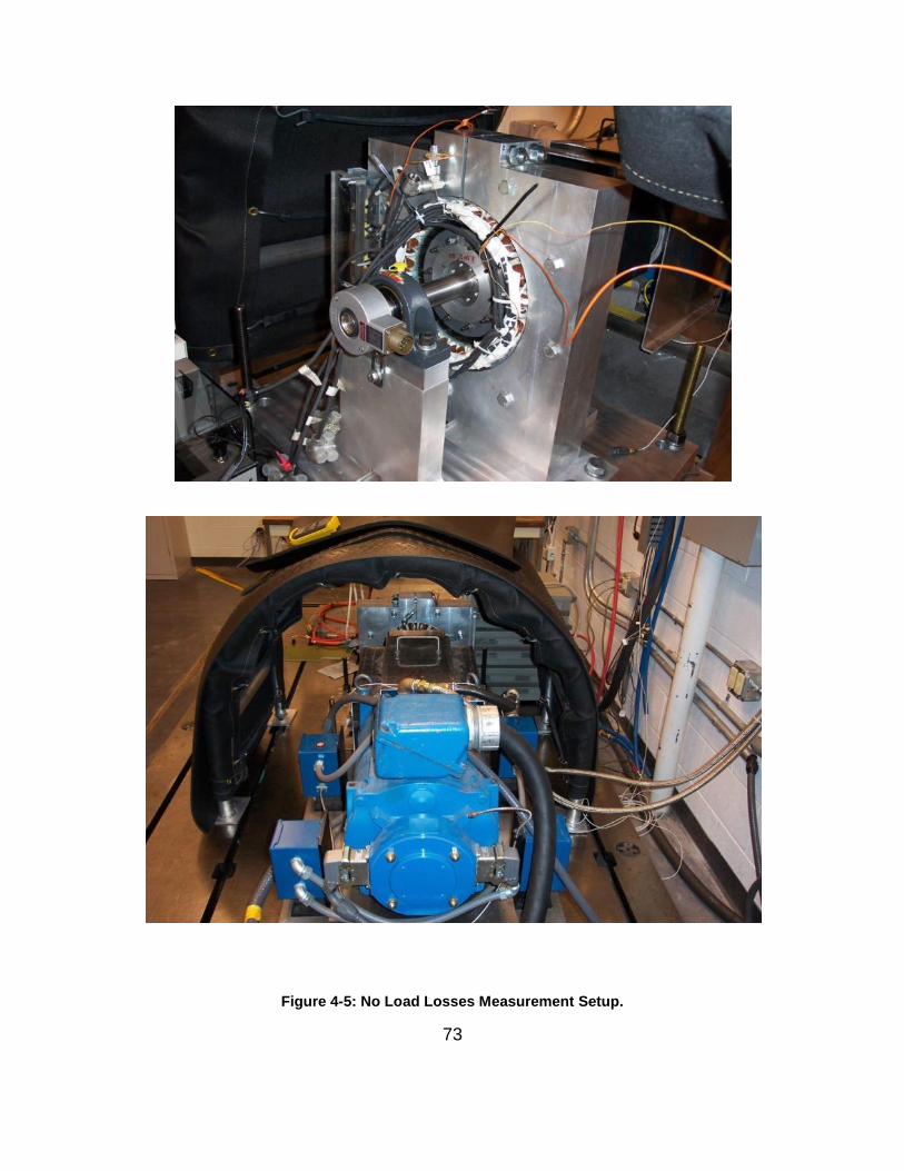
73

Figure 4-5: No Load Losses Measurement Setup.

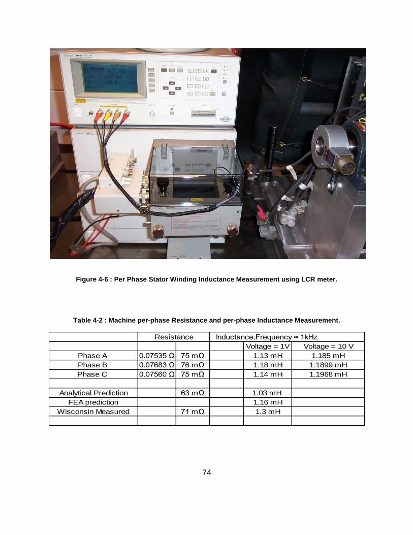
74

Figure 4-6 : Per Phase Stator Winding Inductance Measurement using LCR meter.

Table 4-2 : Machine per-phase Resistance and per-phase Inductance Measurement.

Inductance,Frequency ≈ 1kHz

Voltage = 1V Voltage = 10 V

Phase A 0.07535 Ω 75 mΩ 1.13 mH 1.185 mH

Phase B 0.07683 Ω 76 mΩ 1.18 mH 1.1899 mH

Phase C 0.07560 Ω 75 mΩ 1.14 mH 1.1968 mH

Analytical Prediction 63 mΩ 1.03 mH

FEA prediction 1.16 mH

Wisconsin Measured 71 mΩ 1.3 mH

Resistance

75

Figure 4-7 shows captured back-EMF waveform at base speed (900 rpm) and 4000

rpm. Figure 4-8, Figure 4-9 and Figure 4-10 shows the measured back-EMF with its

Fast Fourier Transform. The purple line is the back-EMF, and the yellow graph is its

FFT. A 3rd harmonic can be noticed on these figures. Stator windings of a three phase

PMSM motor usually have a common neutral point as they are usually connected in Y

format. This type of connection results in the cancelation of 3rd and all the triplen

harmonics. From these figures, it can also be seen that the surface PM motor with

fractional-slot concentrated-windings type motor has sinusoidal shaped back-EMF.

Using the dynamometer, the experimental motor was rotated at 0 – 4000 rpm in the

steps of 100 rpm. At each speed, peak to peak, and RMS value of the fundamental

frequency component of the back-EMF was recorded. Table 4-3 lists all this measured

data.

Figure 4-11 shows measured no-load losses. Figure 4-12 shows RMS values of the

back-EMF along with its least square fit. This is used to calculate the voltage constant

Kv in Equation (3.4). Since there is no load attached to the motor, torque required by the

dyne to keep the motor speed constant is only the no-load power loss ( *P T ) at

that speed.

4.4 Experimental Setup

Figure 4-13 shows a close up of the experimental, 6-kW surface permanent magnet

motor with fractional-slot concentrated-windings.

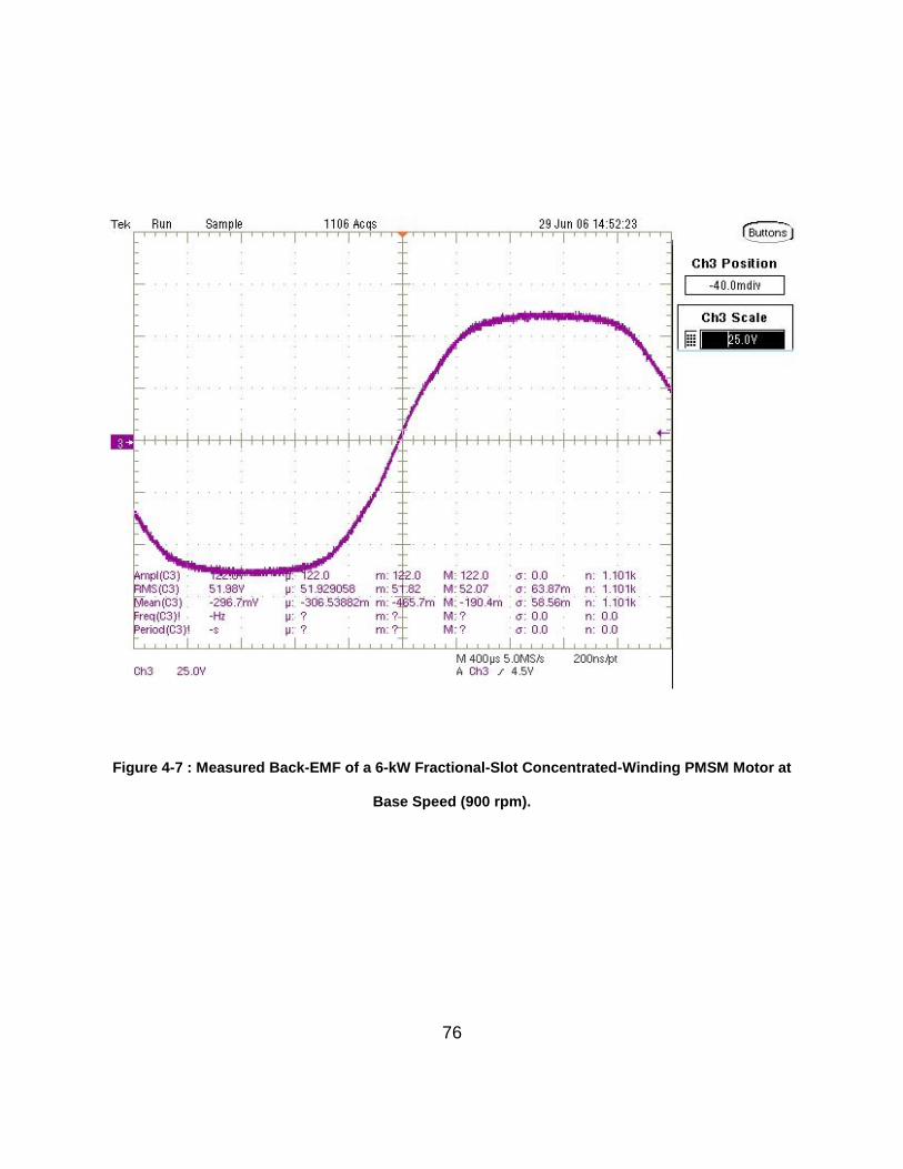
76

Figure 4-7 : Measured Back-EMF of a 6-kW Fractional-Slot Concentrated-Winding PMSM Motor at

Base Speed (900 rpm).

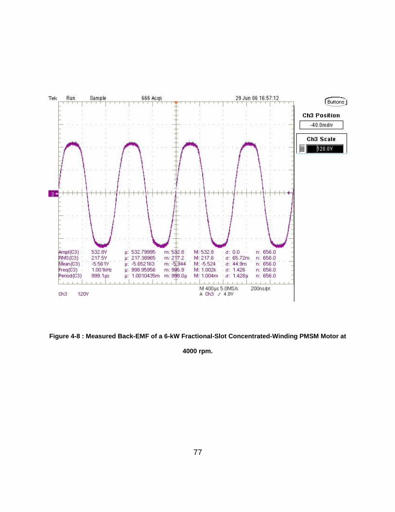
77

Figure 4-8 : Measured Back-EMF of a 6-kW Fractional-Slot Concentrated-Winding PMSM Motor at

4000 rpm.

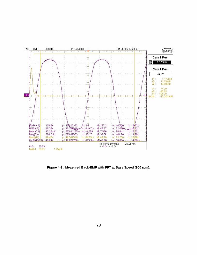
78

Figure 4-9 : Measured Back-EMF with FFT at Base Speed (900 rpm).

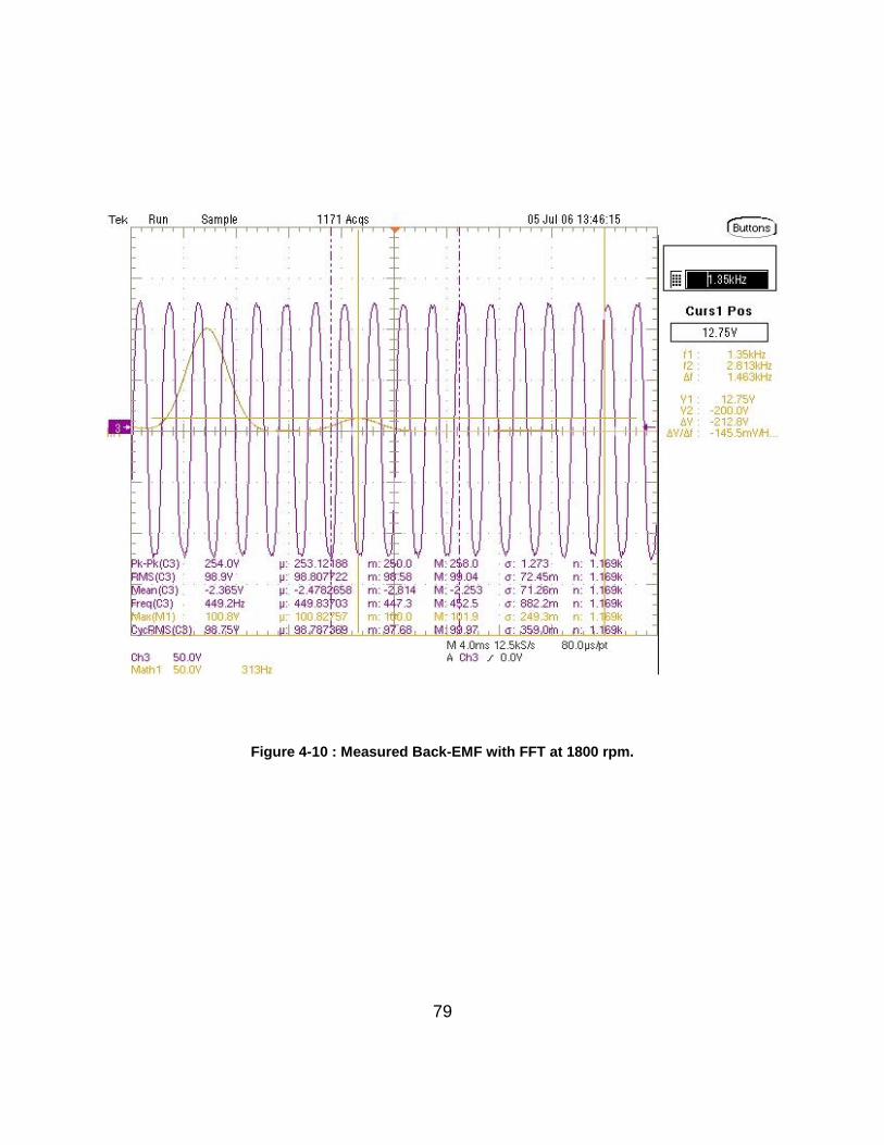
79

Figure 4-10 : Measured Back-EMF with FFT at 1800 rpm.

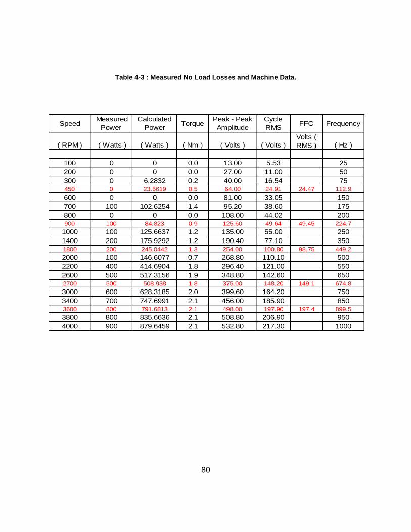
80

Table 4-3 : Measured No Load Losses and Machine Data.

( RPM ) ( Watts ) ( Watts ) ( Nm ) ( Volts ) ( Volts )

Volts (

RMS ) ( Hz )

100 0 0 0.0 13.00 5.53 25

200 0 0 0.0 27.00 11.00 50

300 0 6.2832 0.2 40.00 16.54 75

450 0 23.5619 0.5 64.00 24.91 24.47 112.9

600 0 0 0.0 81.00 33.05 150

700 100 102.6254 1.4 95.20 38.60 175

800 0 0 0.0 108.00 44.02 200

900 100 84.823 0.9 125.60 49.64 49.45 224.7

1000 100 125.6637 1.2 135.00 55.00 250

1400 200 175.9292 1.2 190.40 77.10 350

1800 200 245.0442 1.3 254.00 100.80 98.75 449.2

2000 100 146.6077 0.7 268.80 110.10 500

2200 400 414.6904 1.8 296.40 121.00 550

2600 500 517.3156 1.9 348.80 142.60 650

2700 500 508.938 1.8 375.00 148.20 149.1 674.8

3000 600 628.3185 2.0 399.60 164.20 750

3400 700 747.6991 2.1 456.00 185.90 850

3600 800 791.6813 2.1 498.00 197.90 197.4 899.5

3800 800 835.6636 2.1 508.80 206.90 950

4000 900 879.6459 2.1 532.80 217.30 1000

Cycle

RMSFFC FrequencySpeed

Measured

Power

Calculated

Power Torque

Peak - Peak

Amplitude

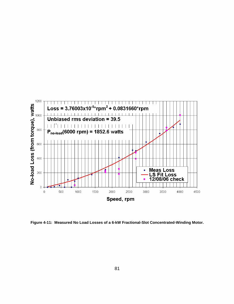
81

Figure 4-11: Measured No Load Losses of a 6-kW Fractional-Slot Concentrated-Winding Motor.

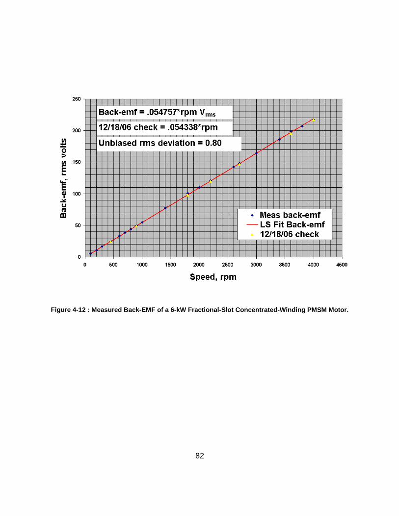
82

Figure 4-12 : Measured Back-EMF of a 6-kW Fractional-Slot Concentrated-Winding PMSM Motor.

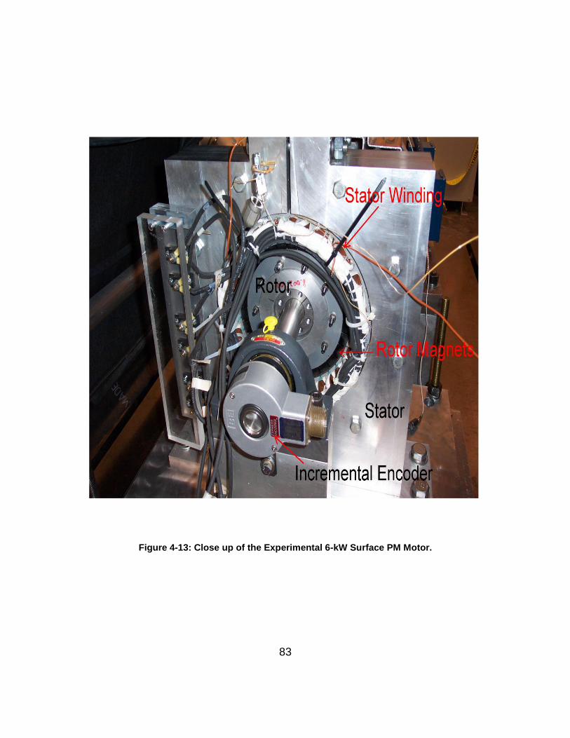
83

Figure 4-13: Close up of the Experimental 6-kW Surface PM Motor.

84

Stator, stator windings, rotor, rotor permanent magnets, and incremental encoder can

be seen in this figure.

It is very important to know the exact rotor position of the synchronous motors because

if the applied stator voltage is 1800 out of phase with the back-EMF, the resulting large

current can damage the motor windings. An incremental encoder was used to measure

the speed and the rotor position of the experimental motor. HS35 type incremental

optical encoder from BEI industry was used. Incremental encoders typically have three

output pulses, namely A, B and Z. This particular encoder has 1024 pulses (A and B)

per mechanical revolution. Because of the offset between pulse A and pulse B, a 4X

resolution can be obtained (by using rising and falling edge of Pulse A and B) to

measure the speed and to estimated the rotor position. There is also one pulse per

mechanical revolution, also called as a reference pulse or a Z pulse. This Z pulse is

usually used to reset the rotor angle measurement counter after 360°.

Figure 4-14 shows these z pulse (pink) along with the generated back-EMF at 900 rpm.

The angle difference between the index pulse and the nearest zero-crossing (with rising

voltage) of the back-EMF is recorded. Since the encoder is fixed on the rotor shaft, this

offset remains constant over the entire speed range. So when the motor is running, Z

pulse is detected by connecting it to the digital input terminal of the OPAL RT system.

An event detection block (hardware + software) was used. When this pulse is detected,

a recorded offset degree from this point gives the zero-crossing of the back-EMF

waveform. This was considered as a zero degrees i.e. 0 .

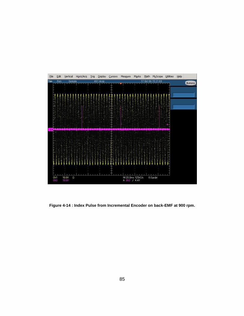
85

Figure 4-14 : Index Pulse from Incremental Encoder on back-EMF at 900 rpm.

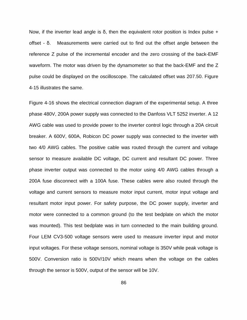
86

Now, if the inverter lead angle is δ, then the equivalent rotor position is Index pulse +

offset - δ. Measurements were carried out to find out the offset angle between the

reference Z pulse of the incremental encoder and the zero crossing of the back-EMF

waveform. The motor was driven by the dynamometer so that the back-EMF and the Z

pulse could be displayed on the oscilloscope. The calculated offset was 207.50. Figure

4-15 illustrates the same.

Figure 4-16 shows the electrical connection diagram of the experimental setup. A three

phase 480V, 200A power supply was connected to the Danfoss VLT 5252 inverter. A 12

AWG cable was used to provide power to the inverter control logic through a 20A circuit

breaker. A 600V, 600A, Robicon DC power supply was connected to the inverter with

two 4/0 AWG cables. The positive cable was routed through the current and voltage

sensor to measure available DC voltage, DC current and resultant DC power. Three

phase inverter output was connected to the motor using 4/0 AWG cables through a

200A fuse disconnect with a 100A fuse. These cables were also routed through the

voltage and current sensors to measure motor input current, motor input voltage and

resultant motor input power. For safety purpose, the DC power supply, inverter and

motor were connected to a common ground (to the test bedplate on which the motor

was mounted). This test bedplate was in turn connected to the main building ground.

Four LEM CV3-500 voltage sensors were used to measure inverter input and motor

input voltages. For these voltage sensors, nominal voltage is 350V while peak voltage is

500V. Conversion ratio is 500V/10V which means when the voltage on the cables

through the sensor is 500V, output of the sensor will be 10V.

87

OffsetOne Rotor

Revolution

Back-EMFIndex Pulse

Position Pulses

Figure 4-15: Rotor Position Estimation.

88

Figure 4-16 : Overall Electrical Schematics.

#4/0 AWG

Good for DC 230 A

Lug 88 is negative

Lug 89 is positive

#12 AWG

# 4/0 AWG

Good for 200

A

Available:

# 1 AWG from Test Bedplate to Building Ground

Motor (6 kW)

Rated current, @ 60 A, on Test Bedplate

Two #1/0 AWG from Robicon frame to

Building Ground

20A Control Logic Power

Supply

3 Phase AC Utility Supply: 480 V, 200 A

20 A Circuit Breaker

Ground wire from Inverter to Test Bedplate - #4/0 AWG in black cable wrapped at ends with Green tape.

U V W Fused breaker: 600V, 200A disconnect with 100A fuse with reducing clips from 200 A to 100 A

Test Bedplate

89 88

G

#1 AWG

Good for 100

A

DC Supply , Robicon

600V , 200 A

Fused Disconnect

Ground wire from Robicon drop to Inverter :

#4/0 AWG wire in orange cable wrapped at ends with Green tape.

Voltage & Current Sensors

89

Four LEM LC300S current sensors were used to measure inverter input currents. For

these sensors, nominal current is 300A while peak current is 500A. Conversion ratio is

1:2000. Additionally, three LEM LT100-P/SP 33 current sensors were used to measure

motor input current (inverter output current).

Figure 4-17 shows the setup of these sensors. The output of these voltage and current

sensors was connected to a power analyzer (Yokogawa PZ4000). Based on the

measured voltage and current information provided by the sensors, this analyzer

computed inverter input power (DC Power) and motor input power (or inverter output

power). The dyne control panel displayed the information about motor output torque and

shaft power. Figure 4-18 shows a view of the overall setup. Figure 4-19 shows an

overall schematic of the same.

The Danfoss VLT 5252 inverter is designed to be used with an induction motor. In order

to use it with the experimental surface PM motor, the inverter’s control logic was

bypassed. Only the switching part along with over-current, over-voltage, over

temperature protection and dynamic braking capability was used. Two sets of interface

cards compatible with the Danfoss inverter were ordered from Aalborg University in

Denmark. One of these cards converted IGBT gate signals (switching information) from

the controller to the fiber optic signal to reduce noise interference. The second card

converted this fiber optic signal back to the digital signals. The second card was

mounted on the inverter. This second card also monitored for over-voltage, over-

current, over-temperature conditions, and if required, could shut down the inverter.

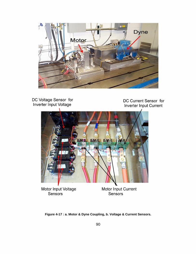
90

Figure 4-17 : a. Motor & Dyne Coupling, b. Voltage & Current Sensors.

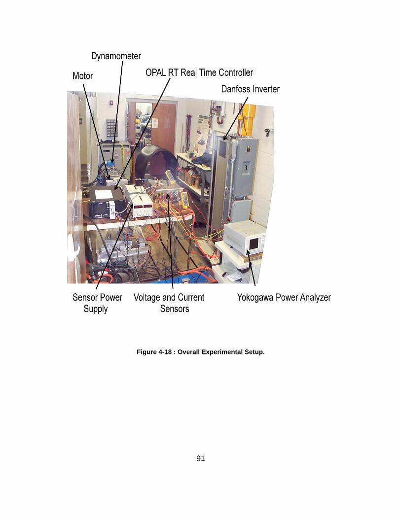
91

Figure 4-18 : Overall Experimental Setup.

92

Figure 4-19 : Overall Test Schematics.

93

Another modification to the Danfoss VLT 5252 was a set of DC connectors, to allow

power from a 600 V, 600 A Robicon DC power supply to be connected directly to the

inverter's DC link. In doing so, the converter part of the Danfoss drive was bypassed.

Although not used during this testing, the inverter DC link can be supplied by 3-phase,

480 V power from AC source which is then rectified and used to charge the DC link.

OPAL RT based real time controller with 3.2 GHz speed (800 MHz bus speed) with a

QNX 6.2 operating system was used. OPAL RT OP5340 card with 16 analog inputs was

used to monitor the stator and rotor, currents and voltages; along with rotor position,

motor speed, DC supply voltage and DC supply current.

OPAL RT OP5311 with 16 digital inputs card was used to monitor Z, A and B

incremental encoder pulses. OPAL RT OP5312 card with 16 digital outputs was used to

send the PWM switching signals to the inverter IGBT’s. These signals were sent to the

Danfoss inverter via the Alborg University interface cards. All these signal conditioning

cards were mounted on the “target” PC which has the QNX based operating system. A

Toshiba laptop was used as a “host” PC to compile and download the control model

generated in the Simulink. This compiled model was then downloaded to the “target” PC

via Ethernet cable from the host PC to the target PC. The host computer was also used

to monitor all the feedback (motor speed, motor voltages, motor currents and DC supply

voltage and current). A GP-IB cable transmitted data from the Yokogawa PZ400 power

analyzer, to a data readout program installed on separate Dell desktop in the control

room.

94

A typical motor (or experiment) startup procedure was:

1. Connect the 3-phase, 480V auxiliary power source to provide the power to the

inverter's internal circuitry followed by a restart using a push button on the Alborg card,

(to clear faults).

2. Turn ON the motor and dyne cooling system.

3. Turn ON the dyne power supply.

4. Compile Simulink based control model in the host PC, and download control model to

the target OPAL RT PC; 5. RUN the controller without enabling inverter gate switching.

6. Connect the DC power supply and increase the applied DC voltage from zero to the

desired DC link value in order to avoid high inrush current.

7. Start the dyne in a speed mode and increase the motor speed to 400 RPM.

8. Set the desired speed command through the host PC, release the dyne by turning

the speed mode OFF and ENABLE the inverter gate signal switching. Once the dyne

speed mode is turned off, OPAL RT controller starts controlling the motor speed. An

absolute type encoder can provide the accurate rotor position. If this type of encoder is

used, PMSM motor can be started from the standstill by the controller alone. With an

incremental type encoder, unless the motor is rotating, the initial rotor position cannot

be detected. Without accurate information about the rotor position, voltage cannot be

applied to a synchronous motor to avoid high inrush current.

95

9. Turn the dyne back ON but in torque mode; 10. Start loading the motor to the desired

load condition.

At this point, the controller should be able to maintain the commanded speed while

developing the required torque.

Figure 4-20 shows the overall OPAL RT control model. SM_Encoder has all the control

logic, data acquisition, and signal conditioning program. SC_Encoder_interface has all

the monitoring blocks. Figure 4-21 shows the inside of SM_Encoder.

Upper portion of the Figure 4-21 is speed and rotor position estimation algorithm. Here

encoder pulses A,B and Z are connected to the digital input card of the OPAL RT

system. An even detection block measures the number of A and B pulses. Note that this

particular encoder produces 1024 pulses per revolution. Based on the encoder

feedback, the rotor position and number of revolutions per minute (RPM) is estimated. Z

pulse or the index pulse is also detected and used to reset the rotor position counter.

This is the speed and rotor position feedback. Middle portion of the Figure 4-21 is a

currents and voltages measurement algorithm. Output of the voltage and current sensor

is connected to the analog input card on the OPAL RT system. Phase voltages and

currents were measured for monitoring purpose only. During simulations, it was

detected that DC voltage value had the greatest effect on the controller. Therefore, only

the DC voltage feedback was used for control purpose. The lower portion of the Figure

4-21, is the actual CPA based controller. Figure 4-22 shows this conventional phase

advancement based controller.

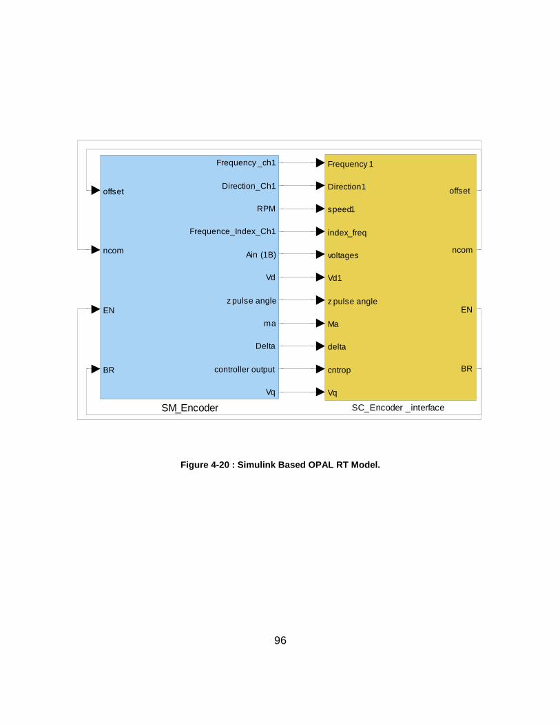
96

Figure 4-20 : Simulink Based OPAL RT Model.

SM_Encoder

offset

ncom

EN

BR

Frequency _ch1

Direction_Ch1

RPM

Frequence_Index_Ch1

Ain (1B)

Vd

z pulse angle

ma

Delta

controller output

Vq

SC_Encoder _interface

Frequency 1

Direction1

speed1

index_freq

voltages

Vd1

z pulse angle

Ma

delta

cntrop

Vq

offset

ncom

EN

BR

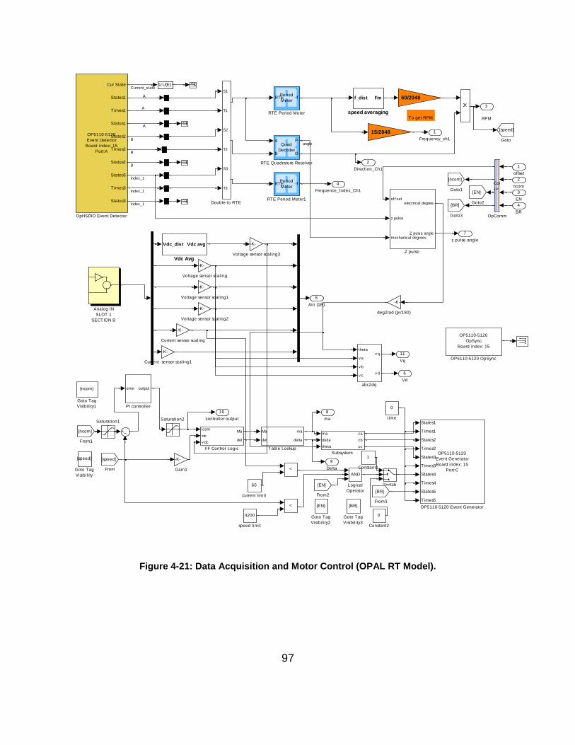
97

Figure 4-21: Data Acquisition and Motor Control (OPAL RT Model).

To get RPM

A

A

11

Vq

10

controller output

9

Delta

8

ma

7

z pulse angle

6

Vd

5

Ain (1B)

4

Frequence_Index_Ch1

3

RPM

2

Direction_Ch1

1

Frequency_ch1

0

time

4200

speed limit

f_dist Fm

speed averaging

-K-

deg2rad (pi/180)

60

current l imit

<

<

theta

v a

v b

v c

v q

v d

abc2dq

of f set

z pulse

mechanical degrees

electrical degree

Z pulse angle

Z pulse

-K-

Voltage sensor scaling3

-K-

Voltage sensor scaling2

-K-

Voltage sensor scaling1

-K-

Voltage sensor scaling

Vdc_dist Vdc avg

Vdc Avg

Ma

del

ma

delta

Table Lookup

Switch

ma

delta

theta

ca

cb

cc

Subsystem

UU(E)

UU(E)

UU(E)

UU(E)

UU(E)

UU(E)

U U(E)

Saturation2Saturation1

A

B

P

D

Quad

Decoder

RTE Quadrature Resolver

RTE fPeriod

Meter

RTE Period Meter1

RTE fPeriod

Meter

RTE Period Meter

error output

PI controller

OP5110-5120

Event Detector

Board index: 15

Port:A

Cur State

States1

Times1

Status1

States2

Times2

Status2

States3

Times3

Status3

OpHSDIO Event Detector

OpComm

Ts = Ts

OpComm

OP5110-5120

OpSync

Board index: 15

OP5110-5120 OpSync

OP5110-5120

Event Generator

Board index: 15

Port:C

States1

Times1

States2

Times2

States3

Times3

States4

Times4

States5

Times5

OP5110-5120 Event Generator

AND

Logical

Operator

60/2048

15/2048

[BR]

Goto3

[EN]

Goto2

[ncom]

Goto1

BR

Goto Tag

Visibil ity3

EN

Goto Tag

Visibil ity2

ncom

Goto Tag

Visibil ity1

speed

Goto Tag

Visibil ity

[speed]

Goto

-K-

Gain1

[BR]

From3

[EN]

From2

[ncom]

From1

[speed]

From

icom

we

v dc

Ma

del

FF Control Logic

S1

T1

S2

T2

S3

T3

Double to RTE

-K-

Current sensor scaling

-K-

Current sensor scaling1

0

Constant2

1

Constant1

Analog IN

SLOT 1

SECTION B

4

BR

3

EN

2

ncom

1

offset

angle

A

B

B

B

index_1

index_1

index_1

Current_state

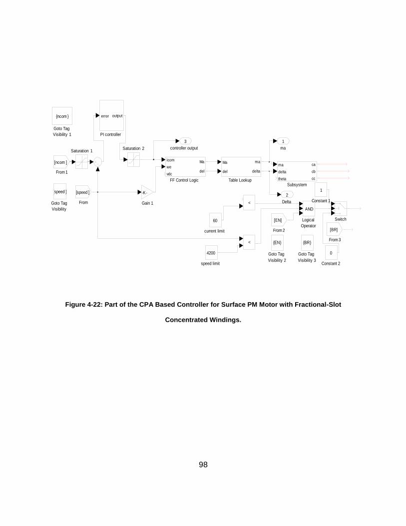
98

Figure 4-22: Part of the CPA Based Controller for Surface PM Motor with Fractional-Slot

Concentrated Windings.

controller output

3

Delta

2

ma

1

speed limit

4200

current limit

60

<

<

Table Lookup

Ma

del

ma

delta

Switch

Subsystem

ma

delta

theta

ca

cb

cc

Saturation 2Saturation 1

PI controller

error output

Logical

Operator

AND

Goto Tag

Visibility 3

BR

Goto Tag

Visibility 2

EN

Goto Tag

Visibility 1

ncom

Goto Tag

Visibility

speed

Gain 1

-K-

From 3

[BR]From 2

[EN]

From 1

[ncom ]

From

[speed ]

FF Control Logic

icom

we

vdc

Ma

del

Constant 2

0

Constant 1

1

99

Here ncom is the speed command set by the operator using the user interface. Speed

feedback is then compared with the desired speed command. Through a PI controller,

this error is converted to a current command. In the constant torque zone (below base

speed), based on the DC voltage feedback, the required current is then converted into

the required modulation index by using Equation (3.30) and required inverter lead angle

by using Equation (3.31). In the constant power region (above base speed), modulation

index is fixed at 4 and the inverter lead angle is calculated by using Equation (3.38).

Figure 4-23 shows the details of the actual Controller. Based the rotor position

feedback, this calculated modulation index and the inverter lead angle is then converted

to the appropriate PWM switching signals. Figure 4-24 shows the details of the sine-

triangle type PWM switching scheme.

As described in Chapter 3, in sinusoidal PMW, a sine wave is compared with the

triangular waveform. The amplitude of the triangular waveform is kept constant. PWM

switching frequency is nothing but the frequency of this triangular waveform. During

experimentation 9 kHz switching frequency was used. Amplitude of the sine waveform

is nothing but the scaled modulation index. Frequency of the sine waveform is same as

the frequency of the motor. Figure 4-24 shows the details for PWM logic.

Angle of the sine waveform is obtained by adding the calculated inverter lead angle to

the measured rotor position. Generated switching signals are then applied to the

Danfoss inverter IGBT’s through an OPAL RT digital output card and Alborg University

interface card.

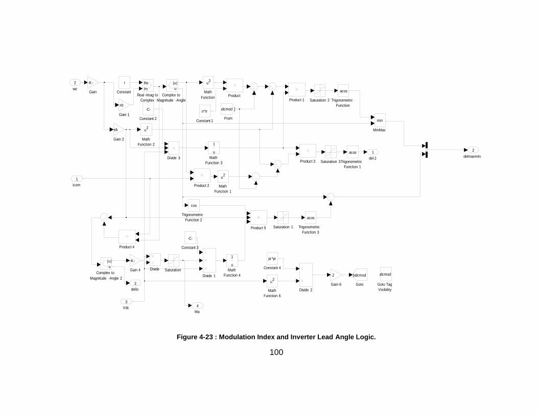
100

Figure 4-23 : Modulation Index and Inverter Lead Angle Logic.

Ma

4

dello

3

delmaxmin

2

del 2

1

Trigonometric

Function 3

acosTrigonometric

Function 2

cos

Trigonometric

Function 1

acos

Trigonometric

Function

acos

Saturation 3

Saturation 2

Saturation 1

Saturation

Real -Imag to

Complex

Re

Im

Product 5

Product 4

Product 3

Product 2

Product 1Product

MinMax

min

Math

Function 6

u2

Math

Function 4

1

u

Math

Function 3

1

u

Math

Function 2

u2

Math

Function 1

u2

Math

Function

u2

Goto Tag

Visibility

vdcmod

Goto

[vdcmod ]

Gain 6

2

Gain 4

-K-

Gain 2

eb

Gain 1

xb

Gain

-K-

From

[vdcmod ]

Divide 3

Divide 2

Divide 1

Divide Constant 4

pi *pi

Constant 3

-C-

Constant 2

-C-

Constant 1

ir*ir

Constant

r

Complex to

Magnitude -Angle 2

|u|

u

Complex to

Magnitude -Angle

|u|

u

Vdc

3

we

2

icom

1

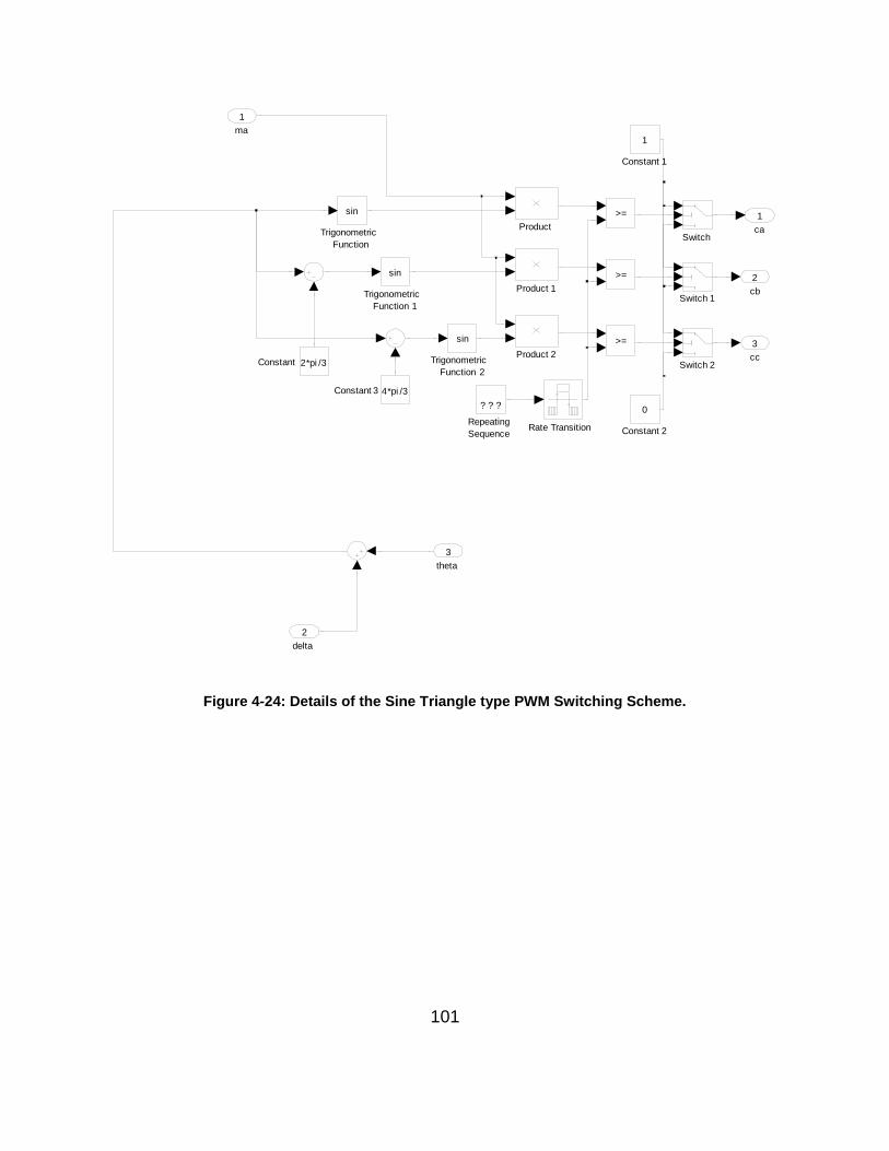
101

Figure 4-24: Details of the Sine Triangle type PWM Switching Scheme.

cc

3

cb

2

ca

1

>=

>=

>=

Trigonometric

Function 2

sin

Trigonometric

Function 1

sin

Trigonometric

Function

sin

Switch 2

Switch 1

Switch

Repeating

Sequence

? ? ?

Rate Transition

Product 2

Product 1

Product

Constant 3 4*pi /3

Constant 2

0

Constant 1

1

Constant 2*pi /3

theta

3

delta

2

ma

1

102

The inverter, then converts available DC voltage from the Robicon DC power supply

into motor input voltage (V ).These phase voltages are then applied to the motor

stator winding leads through voltage and current sensors. Figure 4-25 shows the inside

of SC_Encoder_interface. When the Simulink model is running on the host PC, this is

the only part of the model that is displayed and changed. Through this interface, a

speed command is entered. Desired motor torque can be controlled through Dyne’s

control panel.

4.5 Experimental Results and Conclusion

Tests were carried out at 450, 900, 2000, 3000 and 4000 RPM. For each of these

speeds, applied load was varied from 0% to 100% in the steps of 25%. These sets of

measurements were carried out at 300V DC and at 250V DC. Table 4-4, Table 4-5,

Table 4-6, Table 4-7, Table 4-8, Table 4-9, Table 4-10, Table 4-11 show the measured

torque, stator voltages, stator currents, DC voltage and DC current at each of these test

points.

Figure 4-26 shows the response of CPA based control system to a step change in the

speed. Here the yellow line indicates step change in speed command and the pink

graph indicates the response of the motor. Speed command has been changed from

900 RPM to 1800 RPM.

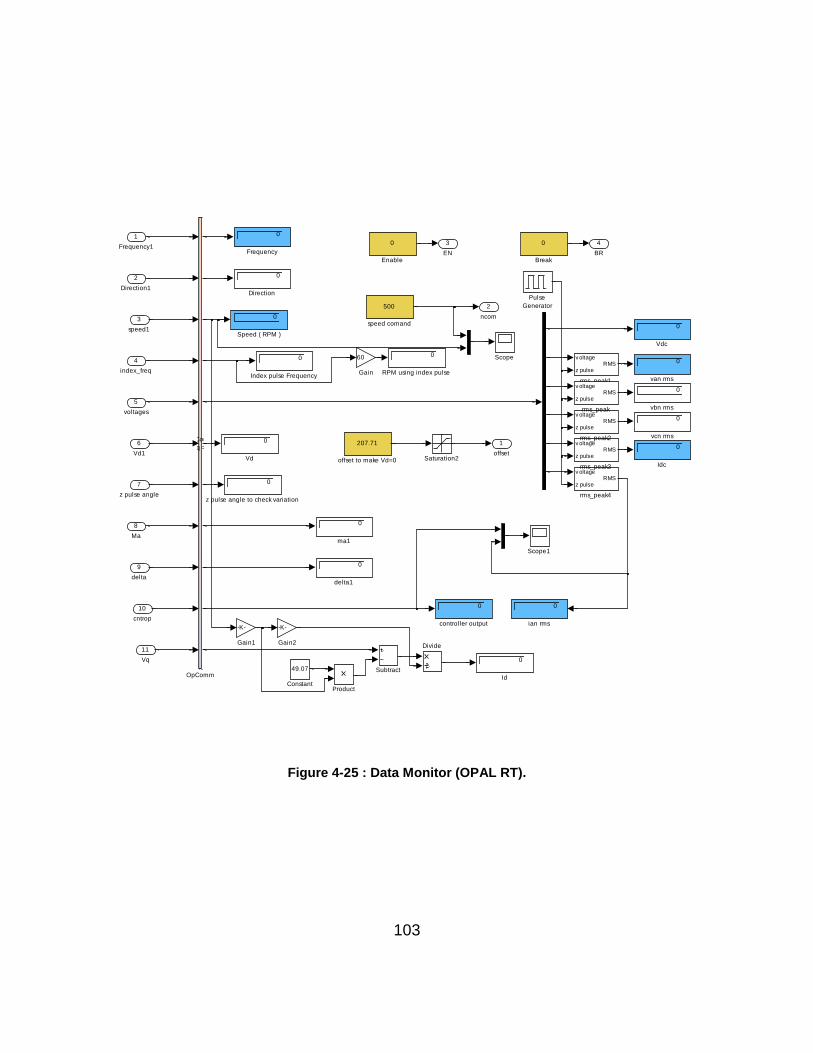
103

Figure 4-25 : Data Monitor (OPAL RT).

4

BR

3

EN

2

ncom

1

offset

0

z pulse angle to check variation

0

vcn rms

0

vbn rms

0

van rms

500

speed comand

v oltage

z pulseRMS

rms_peak4

v oltage

z pulseRMS

rms_peak3

v oltage

z pulseRMS

rms_peak2

v oltage

z pulseRMS

rms_peak1v oltage

z pulseRMS

rms_peak

207.71

offset to make Vd=0

0

ma1

0

ian rms

0

delta1

0

controller output

0

Vdc

0

Vd

Subtract

0

Speed ( RPM )

Scope1

Scope

Saturation2

0

RPM using index pulse

Pulse

Generator

Product

OpComm

Acq = 1

OpComm

0

Index pulse Frequency

0

Idc

0

Id

-K-

Gain2

-K-

Gain1

60

Gain

0

Frequency

0

Enable

Divide

0

Direction

49.07

Constant

0

Break

11

Vq

10

cntrop

9

delta

8

Ma

7

z pulse angle

6

Vd1

5

voltages

4

index_freq

3

speed1

2

Direction1

1

Frequency1

104

Table 4-4 : 250V, 25% Load

25%

MOTOR INVERTER SOURCE

6-kW 36/30 FSCW SPM Danfoss VLT 5252 controlled by Aalborg card interfaced to OPAL-RT Robicon dc supply

RPM

Torque,

N-m

Power,

kW

van,

Vrms ia, Arms

vbn,

Vrms ib, Arms

vcn,

Vrms

ic,

Arms

Power to

Motor,

kW

Measured

Loss, kW

vsupply,

Vdc

isupply,

Adc

Power to

inverter,

kW

450

900 15.9 1498.5 86.93 12.35 86.72 11.99 86.75 12.3 1574 75.5 253.31 6.5 1648

2000 7.2 1507.2 118.4 11.84 118.8 11.13 118.8 12.4 1762 254.8 250.82 7.2 1766

3000 4.8 1508 121.5 11.16 120.9 10.87 121.1 10.2 1899 391 253.11 7.57 1905

4000 3.6 1508 120.7 14.07 125.3 13.48 123.2 14 2226 718 253.23 8.8 2228

105

Table 4-5 : 250V, 50% Load

50%

MOTOR INVERTER SOURCE

6-kW 36/30 FSCW SPM Danfoss VLT 5252 controlled by Aalborg card interfaced to OPAL-RT Robicon dc supply

RPM

Torque,

N-m

Power,

kW van, Vrms ia, Arms

vbn,

Vrms ib, Arms

vcn,

Vrms ic, Arms

Power to

Motor,

kW

Measured

Loss, kW

vsupply,

Vdc

isupply,

Adc

Power to

inverter,

kW

450

900 31.9 3006.5 94.6 21.81 94.79 21.81 94.6 21.78 3073 66.5 253.35 12.73 3197

2000 14.3 2995 118.26 14.03 118.1 14.21 119.04 15.04 3192 197 250.77 12.89 3203

3000 9.6 3016.9 121.06 12.85 121.1 12.92 120.89 12.98 3318 301.1 253.27 12.97 3401

4000 7.2 3015.9 122.34 15.73 121.3 15.9 124.93 15.48 3634 618.1 253.32 14.47 3651

106

Table 4-6 : 250V, 75% Load

75%

MOTOR INVERTER SOURCE

6-kW 36/30 FSCW SPM Danfoss VLT 5252 controlled by Aalborg card interfaced to OPAL-RT Robicon dc supply

RPM

Torque,

N-m

Power,

kW van, Vrms

ia,

Arms

vbn,

Vrms

ib,

Arms

vcn,

Vrms ic, Arms

Power to

Motor,

kW

Measured

Loss, kW

vsupply,

Vdc

isupply,

Adc

Power to

inverter,

kW

450

900 47.7 4500.6 102.72 31.96 102.52 31.8 102.6 32.03 4688 187.4 253.34 19.24 4865

2000 21.5 4500.7 118.56 19.53 117.84 19.92 117.5 19.9 4690 189.3 250.72 18.76 4739

3000 14.4 4522.4 120.68 16.32 120.86 16.14 120.8 16.01 4868 345.6 253.15 19.09 4903

4000 10.8 4523.9 124.15 17.34 122.6 18.21 121.1 18.58 5122 598.1 253.19 20.4 5138

107

Table 4-7: 250V, 100% Load

100%

MOTOR INVERTER SOURCE

6-kW 36/30 FSCW SPM Danfoss VLT 5252 controlled by Aalborg card interfaced to OPAL-RT Robicon dc supply

RPM

Torque,

N-m

Power,

kW van, Vrms

ia,

Arms

vbn,

Vrms

ib,

Arms

vcn,

Vrms ic, Arms

Power to

Motor,

kW

Measured

Loss, kW

vsupply,

Vdc

isupply,

Adc

Power to

inverter,

kW

450

900 63.7 6010.3 111.96 45.44 112 45 111.86 45.1 6406 395.7 252.94 26.28 6623

2000 28.7 6010.9 119.77 22.78 119.6 23.5 119.88 24.16 6138 127.1 253.4 24.43 6179

3000 19.1 6000.4 120.65 20.16 120.5 20 120.5 21.04 6277 276.6 253.02 25.2 6324

4000 14.4 6031.9 120.76 22.26 124 21.2 122.35 22.4 6520 488.1 253.13 26.09 6549

108

Table 4-8 : 300V, 25% Load

25%

MOTOR INVERTER SOURCE

6-kW 36/30 FSCW SPM Danfoss VLT 5252 controlled by Aalborg card interfaced to OPAL-RT Robicon dc supply

RPM

Torque,

N-m

Power,

kW van, Vrms ia, Arms

vbn,

Vrms ib, Arms

vcn,

Vrms ic, Arms

Power to

Motor,

kW

Measured

Loss, kW

vsupply,

Vdc

isupply,

Adc

Power to

inverter,

kW

450 15.9 749.27 81.3 11.61 81.11 11.35 81.04 11.38 784 34.73 300.58 3.03 873

900 16 1508 98.89 12.94 98.89 12.63 98.7 12.74 1609 101 307.73 5.42 1678

2000 7.2 1508 136.79 17.58 134.3 15.58 138.69 16.55 1742 234 302.44 6.13 1842

3000 4.8 1507.5 146.52 7.46 146.3 7.67 146.28 7.7 1942 434.5 307.7 6.43 1938

4000 3.6 1508 150.1 11.52 144.1 12.61 149.33 12.06 2236 728 307.48 7.28 2262

109

Table 4-9 : 300V, 50% Load

50%

MOTOR INVERTER SOURCE

6-kW 36/30 FSCW SPM Danfoss VLT 5252 controlled by Aalborg card interfaced to OPAL-RT Robicon dc supply

RPM

Torque,

N-m

Power,

kW van, Vrms

ia,

Arms

vbn,

Vrms ib, Arms vcn, Vrms ic, Arms

Power to

Motor,

kW

Measured

Loss, kW

vsupply,

Vdc

isupply,

Adc

Power to

inverter,

kW

450 31.8 1498.5 81.56 21.39 81.46 21.45 81.58 21.33 1532 33.5 300.71 5.55 1680

900 31.8 2997.1 103.58 21.8 103.48 21.81 103.38 21.87 3073 75.9 300.57 10.84 3264

2000 14.3 2995 135.77 15.58 134.3 16.78 133.34 15.79 3244 249 302.83 10.85 3285

3000 9.5 2985.5 146.32 10.32 146 10.67 146.08 10.31 3390 404.5 307.7 10.96 3384

4000 7.2 3016.7 148.13 13.3 146.82 13.27 148.34 13.18 3687 670.3 307.4 11.99 3709

110

Table 4-10 : 300V, 75% Load

75%

MOTOR INVERTER SOURCE

6-kW 36/30 FSCW SPM Danfoss VLT 5252 controlled by Aalborg card interfaced to OPAL-RT Robicon dc supply

RPM

Torque,

N-m

Power,

kW

van,

Vrms ia, Arms

vbn,

Vrms ib, Arms

vcn,

Vrms ic, Arms

Power to

Motor,

kW

Measured

Loss, kW

vsupply,

Vdc

isupply,

Adc

Power to

inverter,

kW

450 47.7 2247.8 85.9 36.2 85.86 35.83 85.79 36.09 2537 289.2 300.78 9.42 2841

900 47.7 4495.6 112.9 32 112.79 31.8 112.91 32.04 4645 149.4 300.5 16.33 4926

2000 21.5 4502.9 138.82 19.8 132.09 18.94 135.83 20.81 4702.9 200 302.74 15.65 4747

3000 14.3 4494 146.07 13.42 146.09 13.44 145.84 13.73 4874 380 307.62 15.97 4877

4000 10.7 4483.1 147.24 15.53 148.5 15.91 146.82 15.76 5096 612 307.4 17 5111

111

Table 4-11 : 300V, 100% Load.

100%

MOTOR INVERTER SOURCE

6-kW 36/30 FSCW SPM Danfoss VLT 5252 controlled by Aalborg card interfaced to OPAL-RT Robicon dc supply

RPM

Torque,

N-m

Power,

kW van, Vrms

ia,

Arms vbn, Vrms ib, Arms

vcn,

Vrms ic, Arms

Power to

Motor,

kW

Measured

Loss, kW

vsupply,

Vdc

isupply,

Adc

Power to

inverter,

kW

450 63.7 3001.8 90.86 45.4 90.65 45.17 90.83 45.41 3501 499.2 300.75 12.4 3725

900 63.7 6003.6 120.63 44.7 120.63 44.1 120.74 44.54 6511 507.4 300.26 22.35 6703

2000 28.6 5990 139.62 29 137.83 26.8 135.73 29.21 6195 205 302.52 20.82 6315

3000 19.1 6000.4 145.75 18.7 145.9 18.79 146.03 18.68 6327 326.6 307.62 20.59 6362

4000 14.4 6030.4 146.43 19.4 146.25 20.43 149.36 18.63 6571 540.6 307.35 21.42 6612

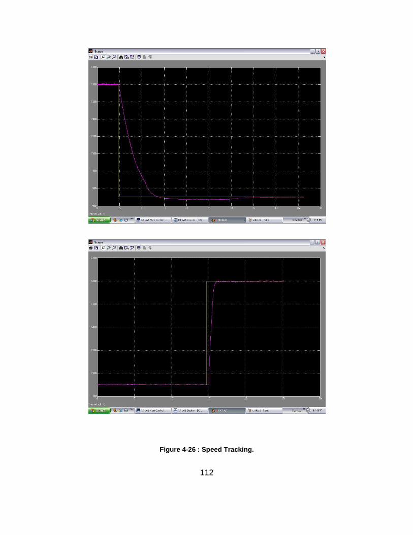
112

Figure 4-26 : Speed Tracking.

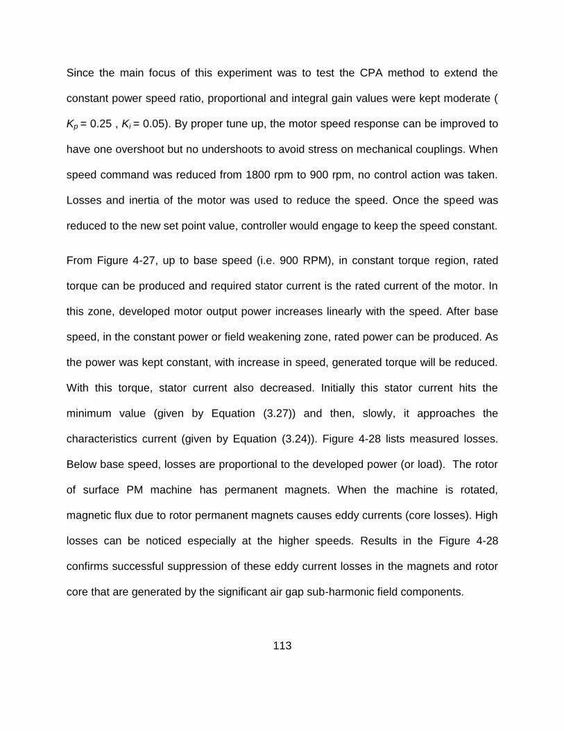
113

Since the main focus of this experiment was to test the CPA method to extend the

constant power speed ratio, proportional and integral gain values were kept moderate (

Kp = 0.25 , Ki = 0.05). By proper tune up, the motor speed response can be improved to

have one overshoot but no undershoots to avoid stress on mechanical couplings. When

speed command was reduced from 1800 rpm to 900 rpm, no control action was taken.

Losses and inertia of the motor was used to reduce the speed. Once the speed was

reduced to the new set point value, controller would engage to keep the speed constant.

From Figure 4-27, up to base speed (i.e. 900 RPM), in constant torque region, rated

torque can be produced and required stator current is the rated current of the motor. In

this zone, developed motor output power increases linearly with the speed. After base

speed, in the constant power or field weakening zone, rated power can be produced. As

the power was kept constant, with increase in speed, generated torque will be reduced.

With this torque, stator current also decreased. Initially this stator current hits the

minimum value (given by Equation (3.27)) and then, slowly, it approaches the

characteristics current (given by Equation (3.24)). Figure 4-28 lists measured losses.

Below base speed, losses are proportional to the developed power (or load). The rotor

of surface PM machine has permanent magnets. When the machine is rotated,

magnetic flux due to rotor permanent magnets causes eddy currents (core losses). High

losses can be noticed especially at the higher speeds. Results in the Figure 4-28

confirms successful suppression of these eddy current losses in the magnets and rotor

core that are generated by the significant air gap sub-harmonic field components.

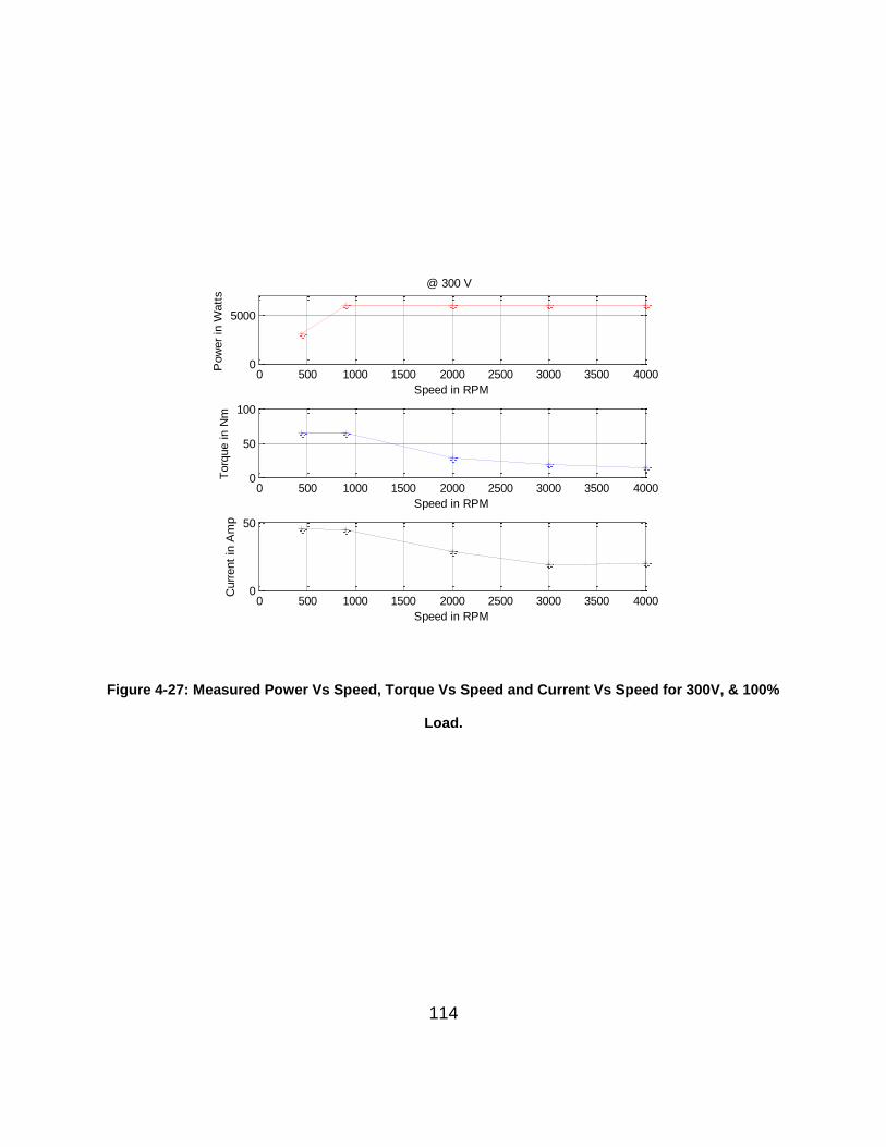
114

Figure 4-27: Measured Power Vs Speed, Torque Vs Speed and Current Vs Speed for 300V, & 100%

Load.

0 500 1000 1500 2000 2500 3000 3500 40000

5000

@ 300 V

Speed in RPM

Pow

er

in W

att

s

0 500 1000 1500 2000 2500 3000 3500 40000

50

100

Speed in RPM

Torq

ue in N

m

0 500 1000 1500 2000 2500 3000 3500 40000

50

Speed in RPM

Curr

ent

in A

mp

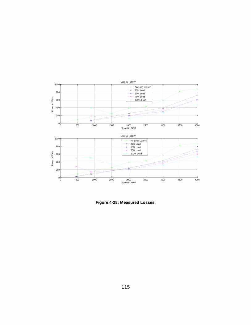
115

Figure 4-28: Measured Losses.

0 500 1000 1500 2000 2500 3000 3500 40000

200

400

600

800

1000Losses : 250 V

Speed in RPM

Pow

er

in W

att

s

No Load Losses

25% Load

50% Load

75% Load

100% Load

0 500 1000 1500 2000 2500 3000 3500 40000

200

400

600

800

1000Losses : 300 V

Speed in RPM

Pow

er

in W

att

s

No Load Losses

25% Load

50% Load

75% Load

100% Load

116

This is a significant result since these losses have been considered to be one of the key

potential obstacles to using fractional-slot concentrated windings for high-speed

operation [27]. Above base speed, as the current approaches the characteristic value,

which is independent of the load condition (or required power output), losses, defined as

the difference between the motor input power and the motor output power, are more for

partial loads. Below base speed losses are proportional to the power output.

Figure 4-29 shows measured inverter efficiency. Below base speed, the inverter is

operating in the linear modulation region. In this region switching losses are high. Above

base speed, inverter operates in the over-modulation region or six-step operation.

Switching waveform is more like a square wave. In this region switching losses are less.

From Figure 4-29 it can be noticed that inverter efficiency is very high in the constant

power region. Between rated base speed and true base speed, inverter operates in the

non-linear region. Here modulation index is between 1 and 4/π. Figure 4-30 shows

measured motor efficiency. In the constant torque region, motor efficiency is good

(above 90%). In constant power region, motor current approaches a constant value.

This value does not depend on the developed shaft power. Current required to produce

25% of the power is almost the same as the current required to produce 100% of the

power. Hence current related losses are almost the same which means partial load

efficiency is poor. This can be seen in the Figure 4-30 and Table 4-12. For the most

operating conditions, motor efficiency is close to 90%. It can be seen that the partial

load efficiency is poor especially at high speed.

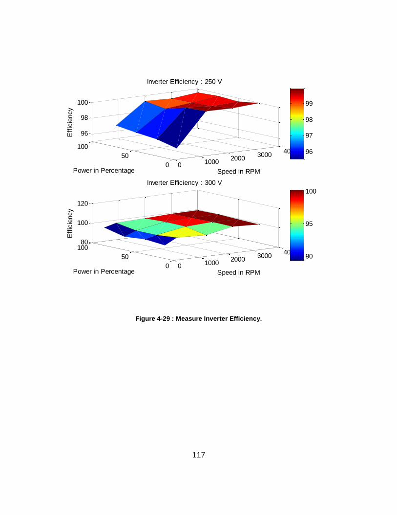
117

Figure 4-29 : Measure Inverter Efficiency.

0 10002000

30004000

0

50

100

96

98

100

Speed in RPM

Inverter Efficiency : 250 V

Power in Percentage

Eff

icie

ncy

96

97

98

99

0 10002000

30004000

0

50

10080

100

120

Speed in RPM

Inverter Efficiency : 300 V

Power in Percentage

Eff

icie

ncy

90

95

100

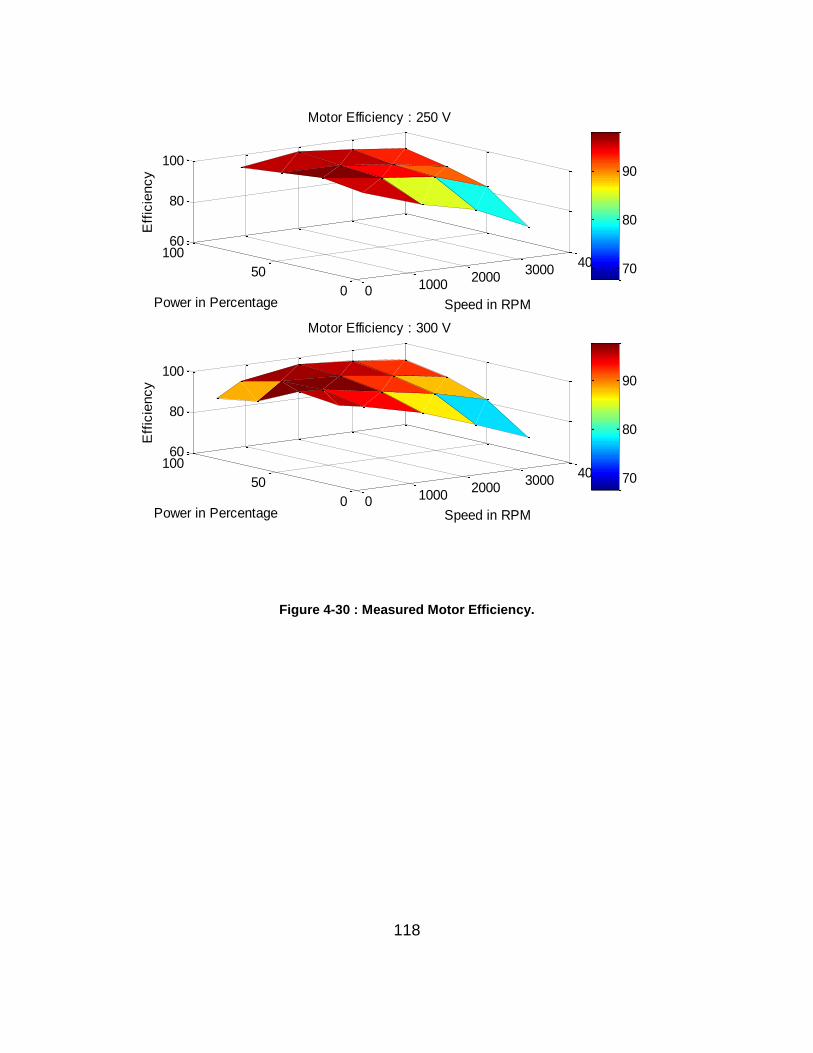
118

Figure 4-30 : Measured Motor Efficiency.

0 10002000

30004000

0

50

10060

80

100

Speed in RPM

Motor Efficiency : 250 V

Power in Percentage

Eff

icie

ncy

70

80

90

0 10002000

30004000

0

50

10060

80

100

Speed in RPM

Motor Efficiency : 300 V

Power in Percentage

Eff

icie

ncy

70

80

90

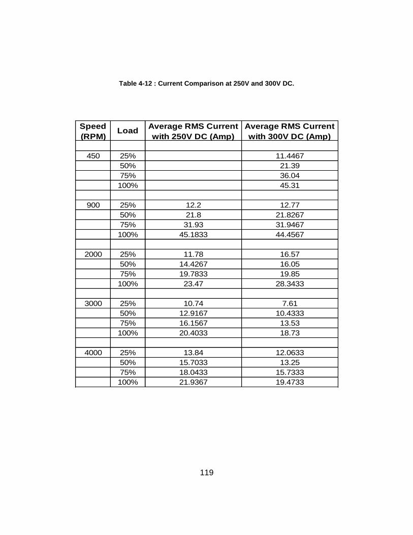
119

Table 4-12 : Current Comparison at 250V and 300V DC.

450 25% 11.4467

50% 21.39

75% 36.04

100% 45.31

900 25% 12.2 12.77

50% 21.8 21.8267

75% 31.93 31.9467

100% 45.1833 44.4567

2000 25% 11.78 16.57

50% 14.4267 16.05

75% 19.7833 19.85

100% 23.47 28.3433

3000 25% 10.74 7.61

50% 12.9167 10.4333

75% 16.1567 13.53

100% 20.4033 18.73

4000 25% 13.84 12.0633

50% 15.7033 13.25

75% 18.0433 15.7333

100% 21.9367 19.4733

Speed

(RPM)Load

Average RMS Current

with 250V DC (Amp)

Average RMS Current

with 300V DC (Amp)

120

In general, even with the traditional vector control schemes, partial load efficiency of the

Surface PM motors, especially at high speeds, is not good [39], [40]. Partial load

efficiency is particularly important if the traction application requires high speed cruising

operation at light loads. For fractional-slot concentrated-windings surface PM machines,

maximizing the power/torque density leads to higher number of poles (experimental

machine has 30 poles). This results in high electrical frequencies [41]. In addition to the

stator core losses + rotor losses, high electrical frequencies generate additional AC

losses in the stator windings of these machines [42], [43], [44].

Care must be taken in the control system itself to reduce these losses. Dual Mode

Inverter control [45] is one method to increase the partial load efficiency of surface PM

machines. This method makes the motor current proportional to the developed power

which increases partial load efficiency. This is done be connecting a pair anti-parallel

thyristors is series with each of the motor phase. Firing of these thyristors can be

controlled to achieve better partial load efficiency. This increases overall reactance

which minimizes the motor current. Traditional vector control can also be modified to

increase the partial load efficiency of the fractional-slot concentrated windings PM

synchronous motors [41]. In this control method, a suitable combination of d-axis

component and a q-axis component of the stator current is estimated by carrying out a

number of simulations or experiments. Figure 4-31 shows measured overall drive

efficiency. Figure 4-32, Figure 4-33, and Figure 4-34 shows comparison of inverter,

motor and drive efficiencies at 250V and 300V DC power supply.

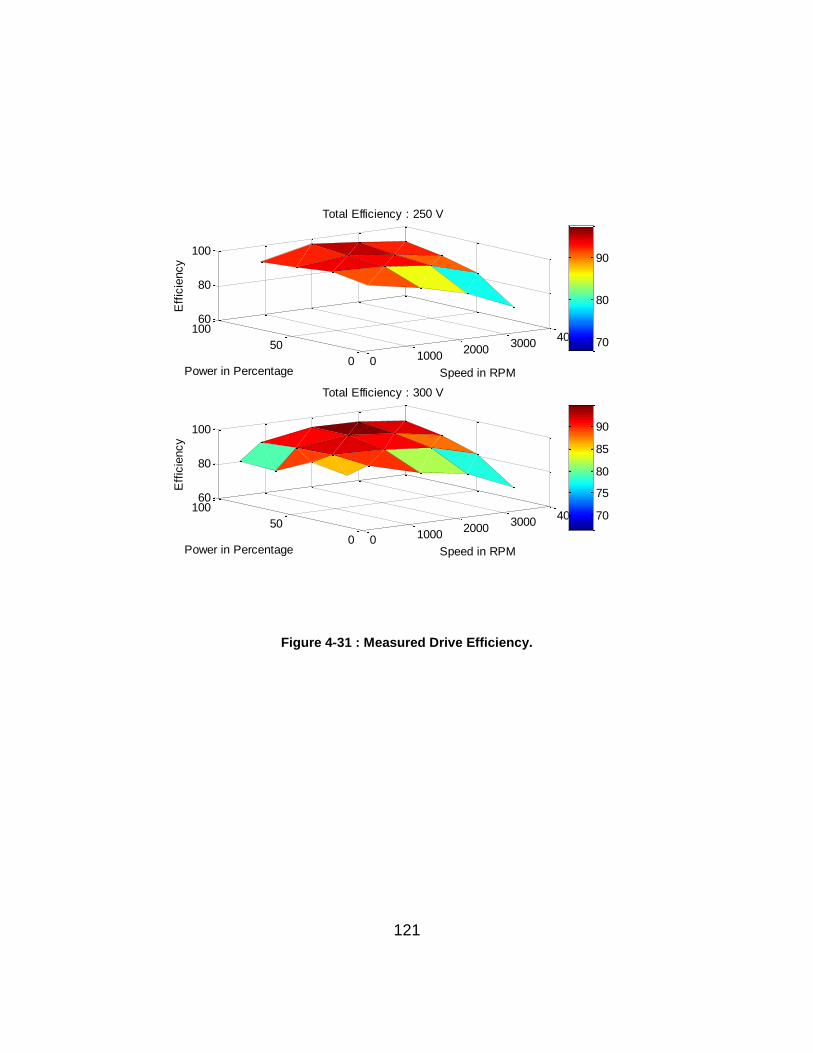
121

Figure 4-31 : Measured Drive Efficiency.

0 10002000

30004000

0

50

10060

80

100

Speed in RPM

Total Efficiency : 250 V

Power in Percentage

Eff

icie

ncy

70

80

90

0 10002000

30004000

0

50

10060

80

100

Speed in RPM

Total Efficiency : 300 V

Power in Percentage

Eff

icie

ncy

70

75

80

85

90

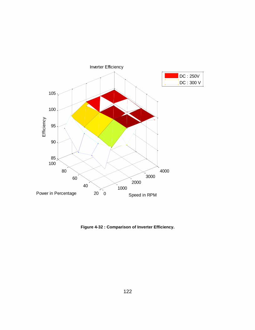
122

Figure 4-32 : Comparison of Inverter Efficiency.

0

1000

2000

3000

4000

20

40

60

80

100

85

90

95

100

105

Speed in RPM

Inverter Efficiency

Power in Percentage

Eff

icie

ncy

DC : 250V

DC : 300 V

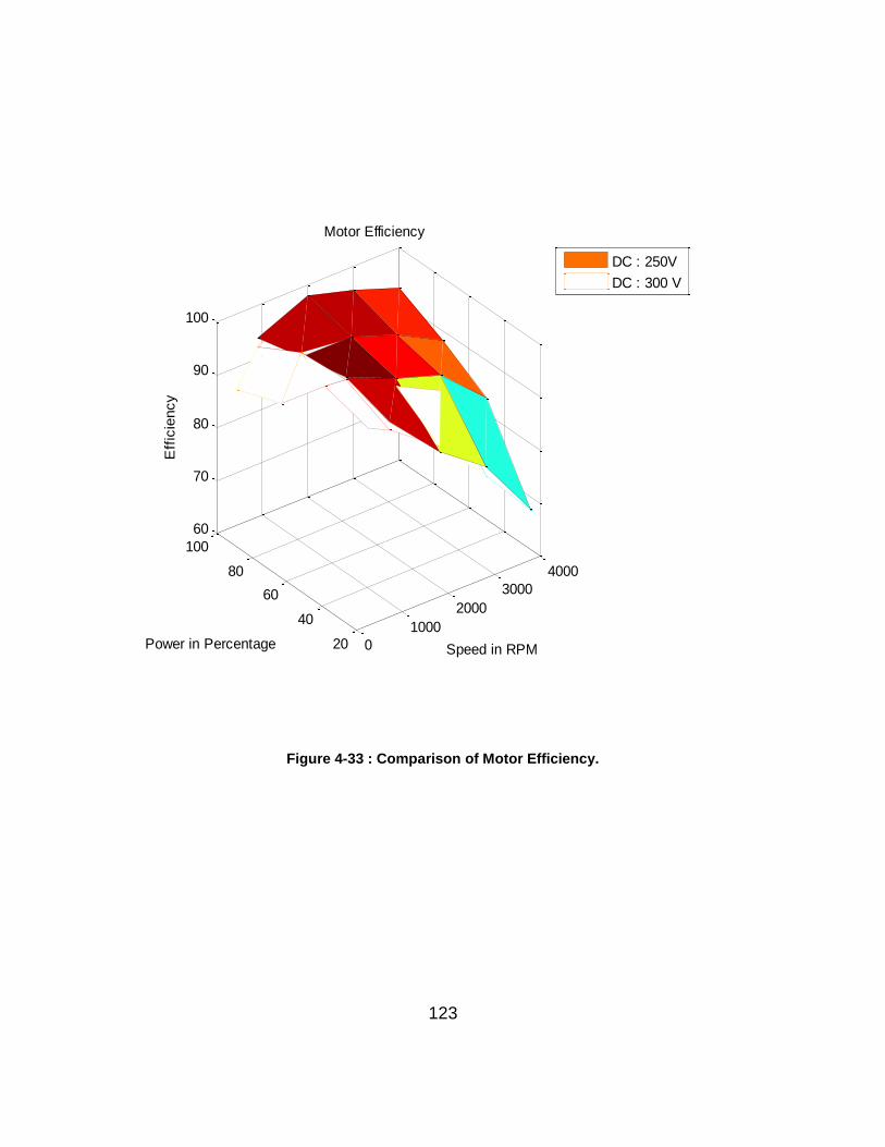
123

Figure 4-33 : Comparison of Motor Efficiency.

0

1000

2000

3000

4000

20

40

60

80

100

60

70

80

90

100

Speed in RPM

Motor Efficiency

Power in Percentage

Eff

icie

ncy

DC : 250V

DC : 300 V

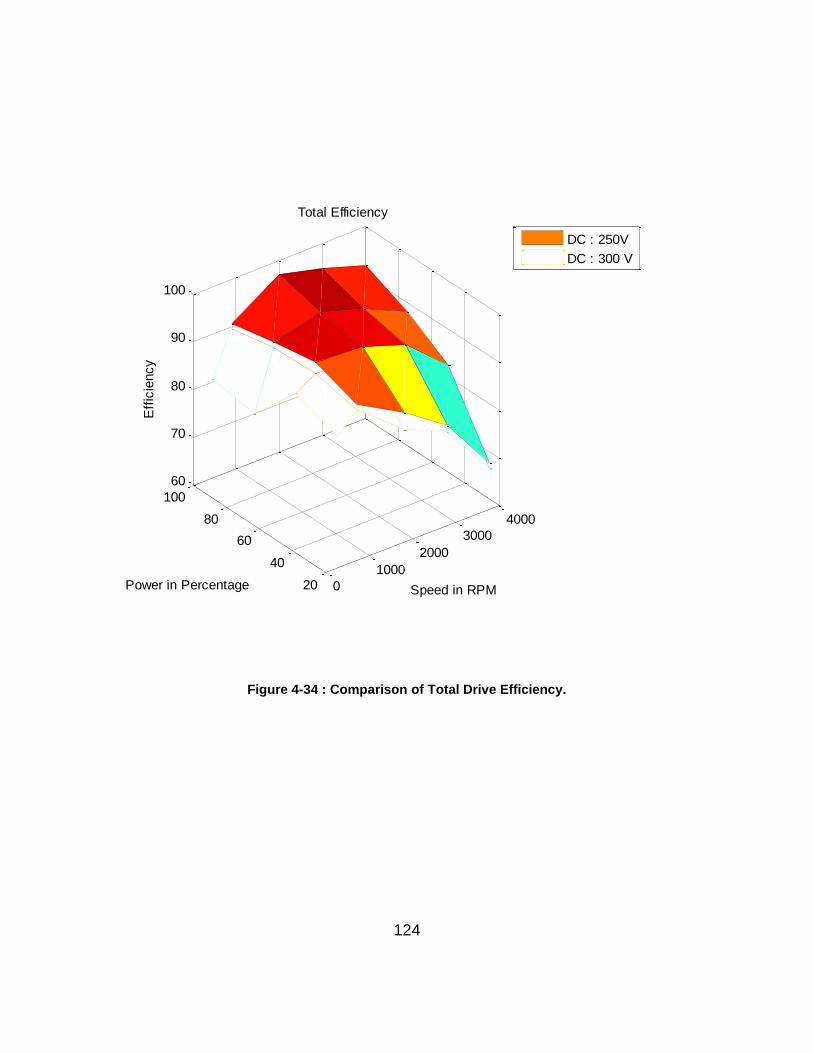
124

Figure 4-34 : Comparison of Total Drive Efficiency.

0

1000

2000

3000

4000

20

40

60

80

100

60

70

80

90

100

Speed in RPM

Total Efficiency

Power in Percentage

Eff

icie

ncy

DC : 250V

DC : 300 V

125

It can be seen from the Figure 4-33 that, for both voltages, motor efficiency is almost

same. Inverter efficiency is also almost same, except for a speed range from base

speed up to the true base speed. Table 4-12 compares stator currents for these two

voltages. It can be seen from the Table 4-12 that, up to base speed, required stator

current is almost equal for 250V and 300V. From rated base speed (900 RPM) till the

nmin , current with 300V DC supply is more than the current with 250V DC supply. So the

current related losses are more with 300V DC supply than 250V DC Supply. Also, note

that for this speed range, sinusoidal PWM operates in the non-linear region.

For the non-linear region, a look up table was used to adjust the modulation index to

avoid unstable operation. This lookup table was designed for a 250V operation. For

300V operation, because of time constrain, same lookup table was used. This can be a

possible reason for more current during the non-linear region with 300V than 250V

power supply. This non-linear region can be avoided by changing modulation index

linearly from 0 to 1 up to the base speed and above base speed operation, the inverter

can be operated in the six-step or square wave operation as reported in [27]. As

expected, above nmin, stator current with 300V DC supply is less than with the 250V

DC supply. So in this speed range, the motor and inverter efficiency should be better

with more voltage. Although as speed increases, stator current approaches to the

characteristic current which does not depend on the applied voltage or the load

conditions.

Figure 4-35 shows the comparison between the no-load losses and motor and drive

efficiency. No load losses were measured in two different ways.

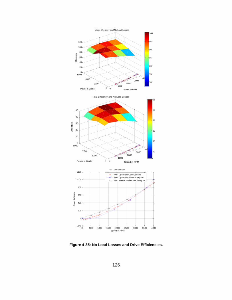
126

Figure 4-35: No Load Losses and Drive Efficiencies.

0

1000

2000

3000

4000

0

2000

4000

6000

0

20

40

60

80

100

120

Speed in RPM

Motor Efficiency and No Load Losses

Power in Watts

Eff

icie

ncy

70

75

80

85

90

95

100

0

1000

2000

3000

4000

0

2000

4000

60000

20

40

60

80

100

Speed in RPM

Total Efficiency and No Load Losses

Power in Watts

Eff

icie

ncy

70

75

80

85

90

95

0 500 1000 1500 2000 2500 3000 3500 4000-200

0

200

400

600

800

1000

1200No Load Losses

Speed in RPM

Pow

er

in W

att

s

With Dyne and Oscilloscope

With Dyne and Power Analyzer

With Inverter and Power Analyzer

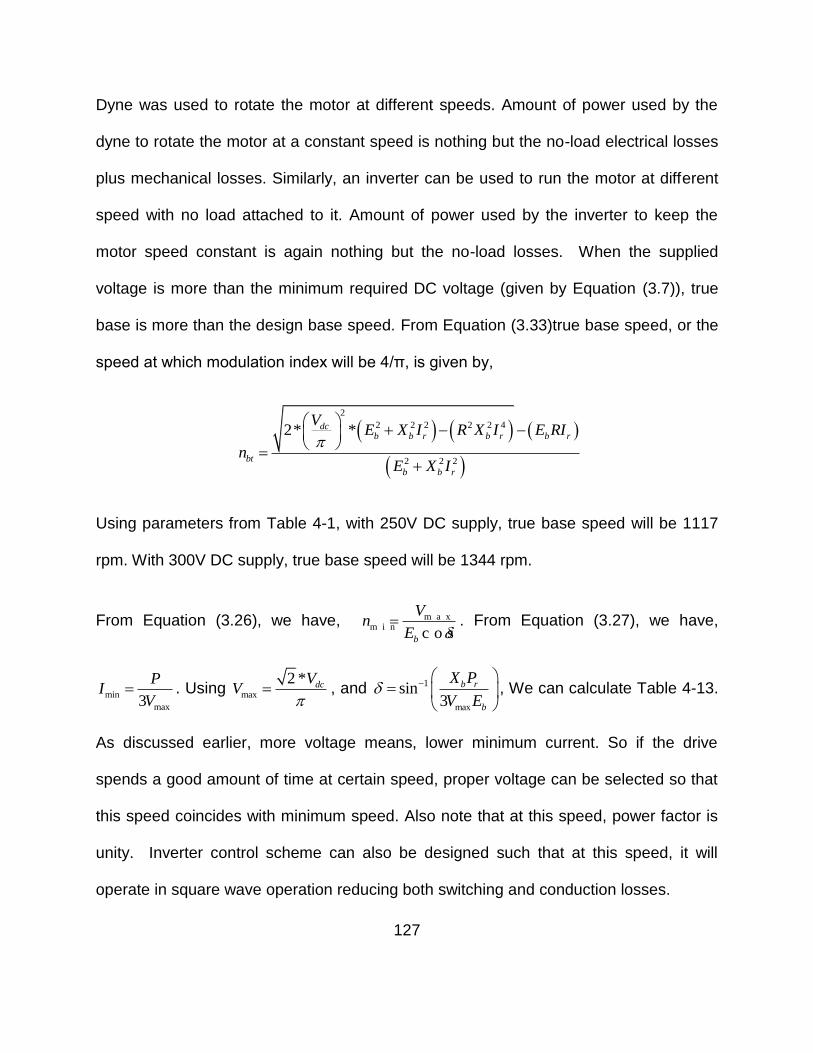
127

Dyne was used to rotate the motor at different speeds. Amount of power used by the

dyne to rotate the motor at a constant speed is nothing but the no-load electrical losses

plus mechanical losses. Similarly, an inverter can be used to run the motor at different

speed with no load attached to it. Amount of power used by the inverter to keep the

motor speed constant is again nothing but the no-load losses. When the supplied

voltage is more than the minimum required DC voltage (given by Equation (3.7)), true

base is more than the design base speed. From Equation (3.33)true base speed, or the

speed at which modulation index will be 4/π, is given by,

2

2 2 2 2 2 4

2 2 2

2* *dcb b r b r b r

bt

b b r

VE X I R X I E RI

nE X I

Using parameters from Table 4-1, with 250V DC supply, true base speed will be 1117

rpm. With 300V DC supply, true base speed will be 1344 rpm.

From Equation (3.26), we have, m a xm i n

c o sb

Vn

E . From Equation (3.27), we have,

min

max3

PI

V . Using max

2 * dcVV

, and 1

max

sin3

b r

b

X P

V E

, We can calculate Table 4-13.

As discussed earlier, more voltage means, lower minimum current. So if the drive

spends a good amount of time at certain speed, proper voltage can be selected so that

this speed coincides with minimum speed. Also note that at this speed, power factor is

unity. Inverter control scheme can also be designed such that at this speed, it will

operate in square wave operation reducing both switching and conduction losses.

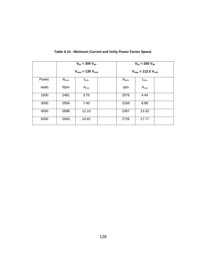
128

Table 4-13 : Minimum Current and Unity Power Factor Speed.

Vdc = 300 Vdc

Vmax = 135 Vrms

Vdc = 250 Vdc

Vmax = 112.5 Vrms

Power,

watts

Nmin,

Rpm

Imin,

Arms

Nmin,

rpm

Imin,

Arms

1500 2481 3.70 2076 4.44

3000 2556 7.40 2169 8.88

4500 2698 11.10 2357 13.33

6000 2943 14.81 2728 17.77

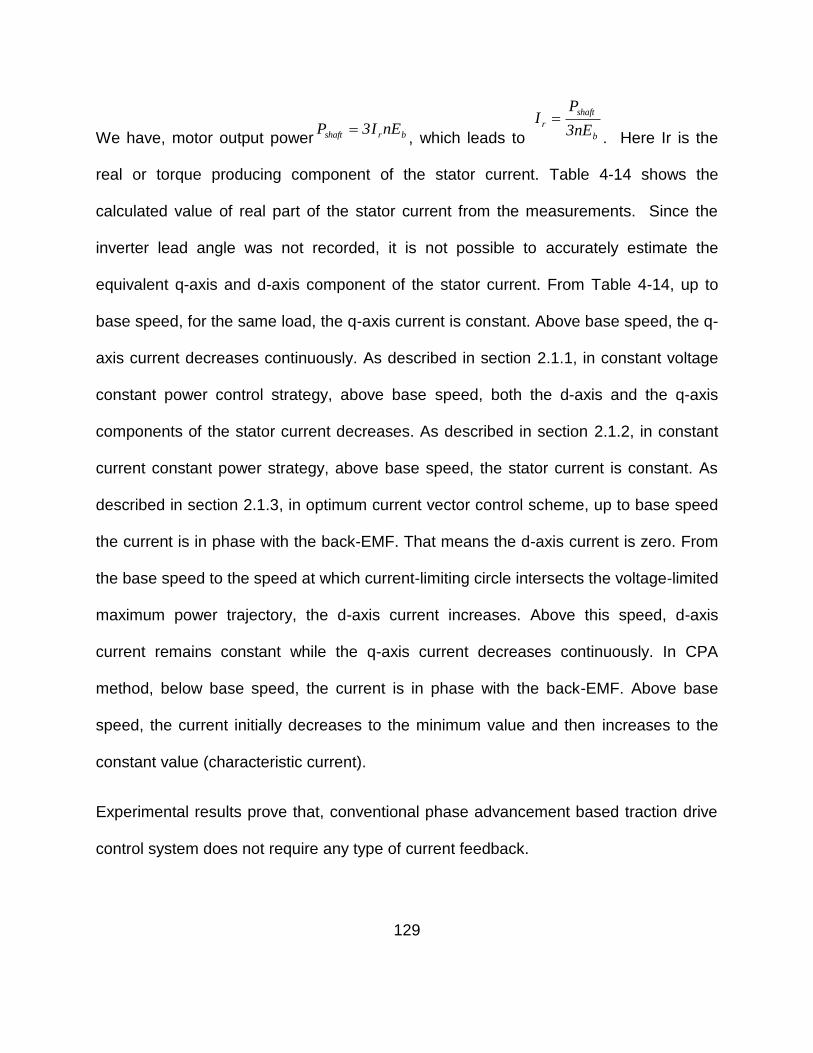
129

We have, motor output power brshaft nEI3P , which leads to b

shaft

rnE3

PI

. Here Ir is the

real or torque producing component of the stator current. Table 4-14 shows the

calculated value of real part of the stator current from the measurements. Since the

inverter lead angle was not recorded, it is not possible to accurately estimate the

equivalent q-axis and d-axis component of the stator current. From Table 4-14, up to

base speed, for the same load, the q-axis current is constant. Above base speed, the q-

axis current decreases continuously. As described in section 2.1.1, in constant voltage

constant power control strategy, above base speed, both the d-axis and the q-axis

components of the stator current decreases. As described in section 2.1.2, in constant

current constant power strategy, above base speed, the stator current is constant. As

described in section 2.1.3, in optimum current vector control scheme, up to base speed

the current is in phase with the back-EMF. That means the d-axis current is zero. From

the base speed to the speed at which current-limiting circle intersects the voltage-limited

maximum power trajectory, the d-axis current increases. Above this speed, d-axis

current remains constant while the q-axis current decreases continuously. In CPA

method, below base speed, the current is in phase with the back-EMF. Above base

speed, the current initially decreases to the minimum value and then increases to the

constant value (characteristic current).

Experimental results prove that, conventional phase advancement based traction drive

control system does not require any type of current feedback.

130

Table 4-14 : Calculated Torque Component of the Stator Current (with 300V DC).

RPMRelative

speed, n

Shaft

Power,

kW

Irms Toruqe

CurrentLoad

450 0.5 749 11.45 10.1 25%

450 0.5 1499 21.39 20.2 50%

450 0.5 2248 36.04 30.3 75%

450 0.5 3002 45.31 40.47 100%

900 1 1508 12.77 10.17 25%

900 1 2997 21.83 20.2 50%

900 1 4496 31.95 30.3 75%

900 1 6004 44.46 40.47 100%

2000 2.222 1508 16.57 4.57 25%

2000 2.222 2995 16.05 9.08 50%

2000 2.222 4503 19.85 13.66 75%

2000 2.222 5990 28.34 18.17 100%

3000 3.333 1508 7.61 3.05 25%

3000 3.333 2986 10.43 6.04 50%

3000 3.333 4494 13.53 9.09 75%

3000 3.333 6000 18.73 12.13 100%

4000 4.444 1508 12.063 2.29 25%

4000 4.444 3017 13.25 4.58 50%

4000 4.444 4483 15.73 6.8 75%

4000 4.444 6030 19.47 9.15 100%

131

This method can extend the constant power region of a surface PM motor with phase

inductance greater than L∞. With the help of speed and rotor position information along

with load requirement, the desired current is calculated by solving a simple fundamental

power transfer equation between two voltages sources (applied voltage and back-EMF).

It can be seen from the experimental results that the rated power can be produced at

any speed above base speed with the required current being less than the rated current

of the motor. Below base speed, both modulation index and voltage angle are changed

while above base speed, only voltage angle is changed. Compared to the traditional

vector control scheme, this method is easy to implement and the required computational

power is less. It was possible to implement a time step of 50 μs and a switching

frequency of 9 kHz.

In the constant power region, since the part of the stator current is used to oppose the

magnetic flux produced by the permanent magnets, improper control technique can lead

to irreversible demagnetization of the rotor permanent magnets.

Use of the permanent magnets on the rotor prevents the use PMSM motors for high

speed application. Since there is always a field excitation, faulted stator phase cannot

be safely isolated to continue the use of motor. For these operating conditions,

Switched Reluctance Motors, described in the next chapter, have advantages over the

PMSM motors.

132

5 INTRODUCTION – SWITCHED RELUCTANCE MOTORS

Light electric or hybrid electric vehicles, such as passenger vehicles, have a modest

constant power speed range (CPSR) requirement of 4 to perhaps 6:1. Such

performance can be achieved with traction drives incorporating a variety of popular

motor types including induction, permanent magnet and switched reluctance machines.

For passenger vehicle applications, the switched reluctance motor (SRM) is often ruled

out based on torque pulsations, mechanical vibration, and acoustical noise despite

recent and on-going research addressing these issues [46]. Traction drives for heavy

vehicles may require a CPSR of 10:1 or more. In addition, heavy vehicles, especially

off-road vehicles, are more tolerant to torque ripple, noise, and vibration. The

potentially low motor/inverter cost of the SRM can make it an attractive candidate for

such applications provided the CPSR can be shown to easily exceed a CPSR of 10:1.

High CPSR means drive can operate at high cruising speed. SRM motors are robust

because of their ability to run under failure conditions [15]. In SRM motors, torque/speed

characteristics is not defined solely by the machine manufacturer hence an extreme

wide range of these characteristics can be obtained by simply alternating control

scheme for phase timings [47]. The switched reluctance motor (SRM) has double

saliency meaning it has a saliency in the stator as well as saliency in the rotor. Figure

5-1 shows a cross sectional view of the four phase 8/6 SRM motor.

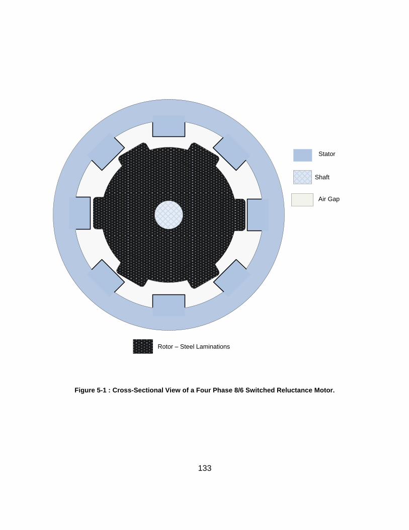
133

Rotor – Steel Laminations

Air Gap

Shaft

Stator

Figure 5-1 : Cross-Sectional View of a Four Phase 8/6 Switched Reluctance Motor.

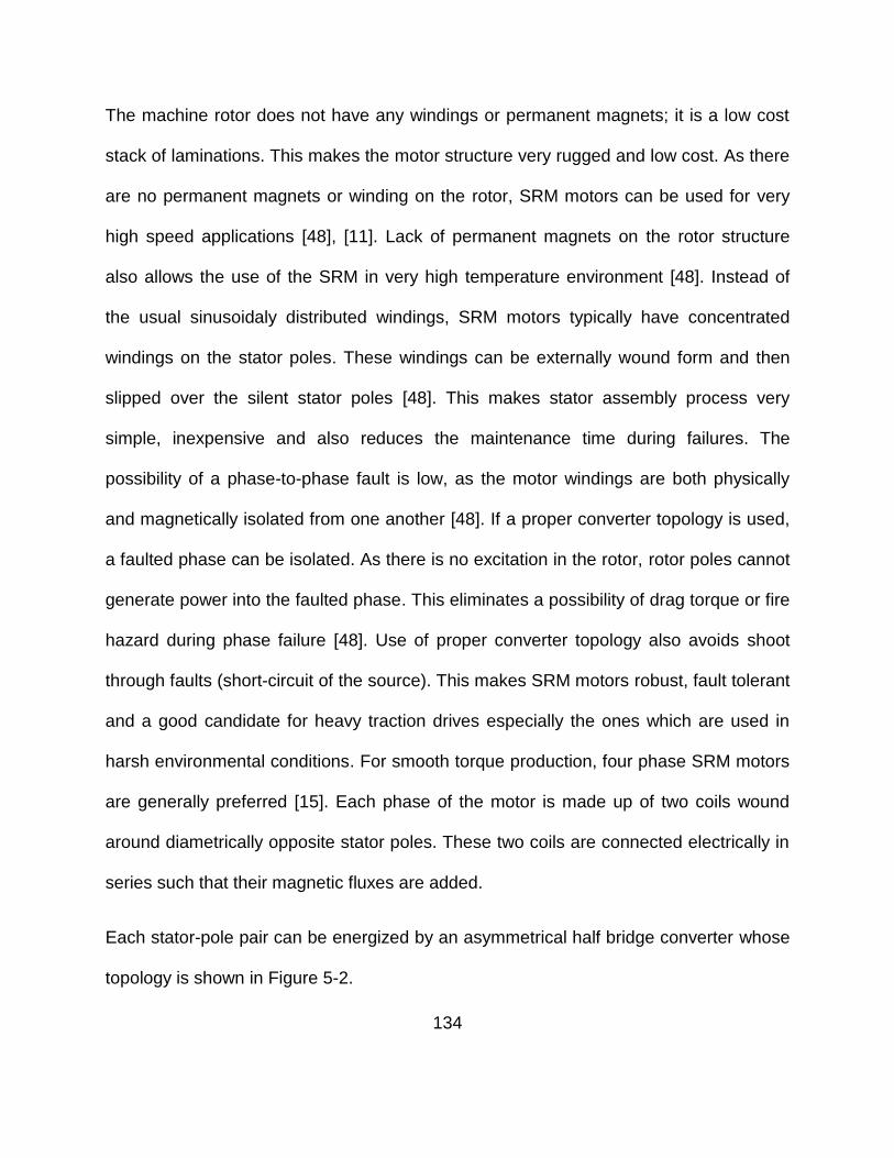
134

The machine rotor does not have any windings or permanent magnets; it is a low cost

stack of laminations. This makes the motor structure very rugged and low cost. As there

are no permanent magnets or winding on the rotor, SRM motors can be used for very

high speed applications [48], [11]. Lack of permanent magnets on the rotor structure

also allows the use of the SRM in very high temperature environment [48]. Instead of

the usual sinusoidaly distributed windings, SRM motors typically have concentrated

windings on the stator poles. These windings can be externally wound form and then

slipped over the silent stator poles [48]. This makes stator assembly process very

simple, inexpensive and also reduces the maintenance time during failures. The

possibility of a phase-to-phase fault is low, as the motor windings are both physically

and magnetically isolated from one another [48]. If a proper converter topology is used,

a faulted phase can be isolated. As there is no excitation in the rotor, rotor poles cannot

generate power into the faulted phase. This eliminates a possibility of drag torque or fire

hazard during phase failure [48]. Use of proper converter topology also avoids shoot

through faults (short-circuit of the source). This makes SRM motors robust, fault tolerant

and a good candidate for heavy traction drives especially the ones which are used in

harsh environmental conditions. For smooth torque production, four phase SRM motors

are generally preferred [15]. Each phase of the motor is made up of two coils wound

around diametrically opposite stator poles. These two coils are connected electrically in

series such that their magnetic fluxes are added.

Each stator-pole pair can be energized by an asymmetrical half bridge converter whose

topology is shown in Figure 5-2.

135

Phase A Phase B Phase CPhase D

QA1

QA2

QB1

QB2

QC1

QC2

QD1

QD2

DA1

DA2

DD1

DD2

QA1

QA2DA1

DA2

VDC

Figure 5-2: Asymmetrical Half-Bridge Voltage Source Inverter Topology for an 8/6 SRM Motor

[11],[15].

136

Here a power electronics switch (IGBT, MOSFET etc.) is connected in between positive

terminal of the DC supply voltage and one end of the stator pole pair winding. A second

switch is connected between the negative terminal of the DC supply voltage and the

other end of the stator pole pair winding. Bypass diodes are also connected across the

stator winding as shown in Figure 5-2. The input DC power supply can be either a

battery or a rectified and filtered AC supply. The DC supply can be fixed or variable in

magnitude. In some known drives, the power supply includes a resonant circuit which

produces a DC voltage which rapidly varies between zero and a predetermined value to

allow zero voltage switching of the power switches [49].

As pointed out by Becerra et. al. in [50], the torque in SRM motor is produced due to the

tendency of a magnetic circuit to align itself to a position of least reluctance. As shown

in Figure 5-2, full DC voltage is applied across the phase winding (phase A) by turning

ON switches QA1 and QA2. This causes current buildup in that phase. This current sets

up a magnetic field which causes a magnetic pull on the nearest rotor pole pair. This

magnetic flux enters the rotor structure through one rotor pole and leaves the rotor

structure through the other pole of that rotor pole pair. That rotor pole pair then aligns

itself to the energized stator pole pair.

This is the position of minimum reluctance (as seen by the stator current). This is also a

position of least stored energy. Once the rotor is at the completely aligned position, both

the switches are turned OFF. This converter also provides a path for continuity of

inductor currents through the bypass diodes when excitation is removed from a coil.

137

All machine phases are excited sequentially and synchronously with the help of a rotor

position encoder to produce unidirectional torque. Torque in the SRM is developed as a

solenoidal force as opposed to the Lorentz force that drives most motors, where both

the stator and rotor produces magnetic field [51].

5.1 Modeling of Switched Reluctance Motors [4][51].

Coupling between phases of the SRM is weak [15], allowing model of each phase to be

developed and solved independently. For one phase, we have coil terminal voltage,

( , )

s

d iV iR

dt

, (5.1)

Here, Vs = voltage applied to the winding by the converter, i = winding current, =

magnetic flux linkage of the winding, R = winding resistance, and = rotor position.

Equation (5.1) is nonlinear due to the nonlinear dependence of the flux linkages , on

the rotor position , and the winding current i . The differential equation can be

expanded as,

( , ) ( , )

s

i di i dV iR

i dt dt

(5.2)

Where ddt

i.e. the motor speed in rad/sec, and we have,

138

( , ) ( , )

s

i di iV iR

i dt

(5.3)

Defining incremental inductance,

,,

il i

i

(5.4)

and pseudo back-EMF,

,, , .

ie i

(5.5)

we have,

( , ). , ,s

diV iR l i e i

dt (5.6)

The term , ,e i

is called as a pseudo back-EMF because, unlike surface PM Motors,

not all of the instantaneous power associated with , ,e i

is converted to the

mechanical form.

Some part of this power is a stored energy, associated with the charge and discharge of

the coil inductance, and rest is converted to mechanical form. The stored energy

component has a zero average value. From the Equation(5.6), we can write the per

phase equivalent circuit of SRM as shown in the Figure 5-3.

139

v

i

R ,l i

, ,e i

+

-

Figure 5-3: Per Phase Equivalent Circuit of Switched Reluctance Motor.

For the simplicity of initial analysis, saturation of magnetic flux-linkage is ignored.

Incremental inductance, which depends on both the rotor position and current, can be

considered as a linear inductance which depends only on the rotor position. Equation

(5.3) and (5.6) can be modified to the following form.

, s

di dLV iR L i

dt d

(5.7)

Multiplying by current i, we get,

2 2

s

di dLV i i R Li i

dt d

(5.8)

From the Figure 5-3, power converted to mechanical form is,

140

mP = Power Supplied – Resistive Loss – Power Stored in an Inductor. Therefore,

2 21

2m s

dP V i i R Li

dt

(5.9)

Here ,

2 2

2 2

1 1

2 2

1 1

2 2

d di dLLi Li i

dt dt dt

d di dLLi Li i

dt dt d

(5.10)

After substituting the Equations (5.8) and (5.10) into the Equation (5.9), we get,

2

2

1

2

1

2

m

mm

dLP i

d

P dLT i

d

(5.11)

From above equation, it is clear that torque ( mT) does not depend on the direction of the

stator current (because of square term) and can only be developed when the

inductance changes. Motoring torque can only be produced in the direction of rising

inductance. The shape and magnitude of the produced torque depends mainly on the

shape and magnitude of the phase current. Therefore the torque control in switched

reluctance drives is attained through the current control [52]. Figure 5-4 shows per

phase inductance profile with respect to the rotor angular position and required stator

current profile to produce the motoring torque.

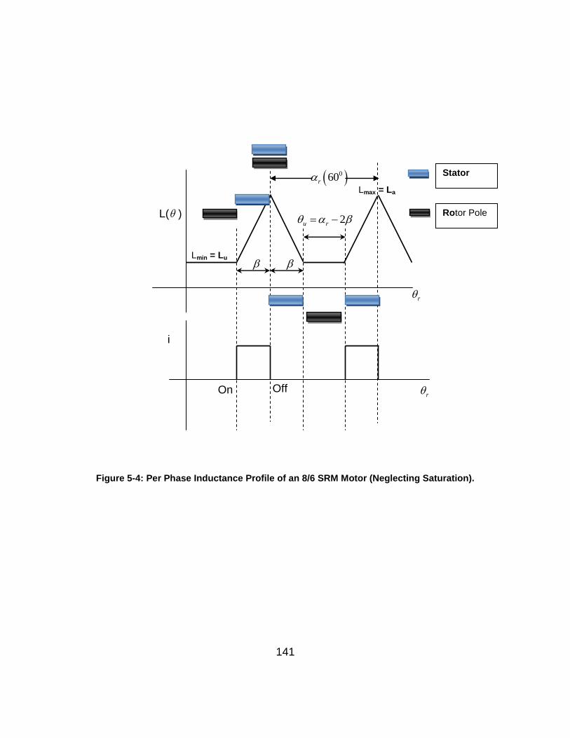
141

Figure 5-4: Per Phase Inductance Profile of an 8/6 SRM Motor (Neglecting Saturation).

L( )

i

r

r

On Off

060r

2u r

Stator

Pole

Rotor Pole

Lmax = La

Lmin = Lu

142

Here saturation is neglected. When a rotor pole pair is aligned with the stator pole pair,

it is a minimum reluctance (or maximum inductance) position for that phase. This

position is also called as a “completely aligned” position. When the center of the rotor

pole pair is aligned with the center line between two adjacent stator pole pairs, this is

the maximum reluctance (or minimum inductance) position. This position is also called

the “completely unaligned” position. If rN is the number of rotor poles, then the rotor pole

pitch,

2

r

rN

(5.12)

This evaluates to be 060 for an 8/6 SRM motor which means the per phase inductance

profile repeats itself every 600. We have, s = stator pole arc length and r = rotor pole

arc length. These lengths are assumed to be equal (i.e. s r ). Inductance profile

for other phases can be obtained by delaying this profile by,

1 12 ,

1 12

6 8 12

r sN N

(5.13)

i.e. by 150,300 and 450. Here Ns is the number of stator poles. As it can be seen in

Figure 5-4, dL d changes sign at full alignment, therefore the pseudo back-EMF

, ,e i also changes its sign at the full alignment.

143

The torque equation can be rewritten as follows,

2 2 max min1 1

2 2e

L LdLT i i

d

(5.14)

Since the current switching to produce torque is based on the reluctance profile, this

machine is called as a switched reluctance motor [4]. Figure 5-4 also shows the ideal

current profile required to produce motoring torque. A current pulse is applied when the

rotor pole pair starts aligning with the stator pole pair (i.e. when magnetic overlap

begins). The current pulse is removed at the completely aligned position. This is done to

avoid generation of braking torque (negative torque). As shown later, a significant

amount of magnetic saturation can be observed especially around completely aligned

position. Because of magnetic saturation, per phase inductance depends not only on

the rotor position but also on the amount of current in the stator winding. Equation (5.14)

is only valid for unsaturated conditions. Considering saturation, the most accurate way

to calculate average power is to rewrite (5.1) as,

,d i v iR dt (5.15)

Then multiplying by phase current and integrating over an interval of T, the total

average power developed by all four phases is given by ,

0

0

average power converted to mechanical form

4= ( )

T

4

m

T

T

P

i v iR dt

i dT

(5.16)

144

The minimum-averaging interval corresponds to one rotor pole pitch, i.e. 60o or / 3

radians for an 8/6 motor. With the substitution,

3

T

(5.17)

Equation (5.16) becomes,

/3

0

/3

0

12

12

12

m

mm

P i d

PT i d

W

(5.18)

Where

/3

0 W i d

(5.19)

is the work done in moving one pole pitch and is also called as the co-energy. The co-

energy W is shown graphically in Figure 5-5.

It is the area enclosed by a plot of current i t vs. flux-linkage t . No saturation can

be observed ff the rotor is held constant at completely unaligned position (i.e. in

between two stator poles), and increased current will be a straight line (OAE) on i t vs.

t plot. Saturation is not observed, as the winding reluctance (mainly due to the air) is

at maximum possible value. With rotor held at completely aligned position, i t vs. t

will follow the path OCF. Since the winding reluctance is at minimum possible value,

saturation can be observed.

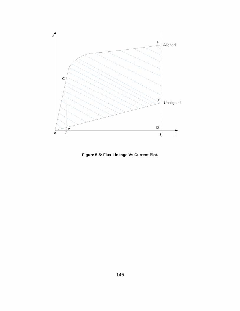
145

oA

C

D

E

F

1I2I i

Unaligned

Aligned

Figure 5-5: Flux-Linkage Vs Current Plot.

146

Now suppose the rotor pole is at completely unaligned position and current (I2) is

applied to the adjacent stator coil. Since the reluctance is at maximum, current will

increase slowly and it will set up magnetic flux. This will cause the rotor pole to move in

to minimum reluctance position (i.e. aligned position).

During this rotor movement, graph will follow the path OAE. Full DC voltage is applied

across that particular phase such that, by the time rotor moves to the on-set of

alignment position, stator current will rise to the required (or rated) value. At point E (at

on-set of alignment), magnetic overlap will start i.e. the rotor pole will start aligning with

the stator pole. Now from point E to point F, the current can be held constant to the

desired value to produce desired torque during the increasing inductance region. Point

F is the fully aligned position. At this point, both the switches are turned OFF. As there

is still current in the phase winding, negative DC voltage needs to be applied through

the bypass diodes. Current will start decreasing and it will follow FCO path. If there is

still current at complete alignment position, reversed back-EMF will reduce current more

rapidly. During alignment, due to the low reluctance saturation can be observed (path

FCO). For a given peak current, maximum torque that can be produced is determined

by the area between the aligned and unaligned flux linkage curves (OAEFCO).

In general, the average torque produced over one revolution is,

avg

r

WT q

(5.20)

Here, q is the number of phases and W is the co-energy. In general, control of the

switched reluctance motor requires; when to turn on the switches (i.e. an advance

147

angle), when to turn off the switches (i.e. dwell angle), and amount of current (current

regulator set point Iset ).

Next chapter describes this SRM control especially high speed control. Switched

Reluctance Drives Limited holds a number of patents (including high speed control) on

different SRM control strategies. Interested readers can refer to [53], [54], [55], [56],

[57], [58].

148

6 LITERATURE REVIEW – SWITCHED RELUCTANCE MOTOR CONTROL

Control requirements for four-quadrant operation can only be met by high-speed real-

time controllers which operate with phase currents directly. Desired average torque can

be obtained by controlling when the current pulse is applied, when the current pulse is

removed and how much current is applied. This can be done by setting an advance

angle adv, a dwell angle dwell

and a current regulator set point seti [15], [12], [11]. For an

advance angle and a dwell angle selection, the point at which magnetic overlap starts is

taken as a reference point. This is the point at which stator pole and rotor pole are at the

on-set of alignment. Since it takes finite amount of time for current to rise (due to the

winding impedance and back-EMF), the current pulse is applied in advance to this point,

such that the current reaches the desired peak value ( setI) just before this magnetic

overlap position. For example, in Figure 6-1, Phase A can be energized by turning on

power electronics switches QA1 and QA2 at an advance angle adv. This applies full DC

supply voltage across the phase A stator winding. During the constant inductance

region, i.e. when the rotor pole is in between two adjacent stator poles, the generated

back-EMF , ,

, , * * *i L i

e i i

is low or zero. So the current rise

is rapid, causing increasing magnetic flux to be established in the machine. This region

is called the “fluxing” region.

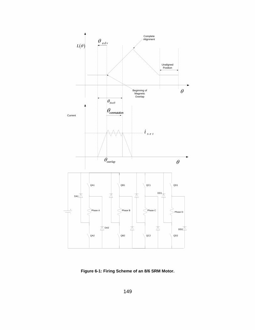
149

overlap

Current

L

s e ti

a d v

dwell

Complete

Alignment

Beginning of

Magnetic

Overlap

Unaligned

Position

commutation

Phase A Phase B Phase CPhase D

QA1

QA2

QB1

QB2

QC1

QC2

QD1

QD2

DA1

DA2

DD1

DD2

Figure 6-1: Firing Scheme of an 8/6 SRM Motor.

150

The magnetic flux produced in the air gap acts on the rotor poles to produce a motoring

torque. This is due to the tendency of the magnetic circuit to align itself to the minimum

reluctance (maximum inductance) position.

As long as the inductance remains nearly constant, there is no or little back-EMF and

full supply voltage is available to force the increasing current. When rotor pole starts

aligning with the stator pole, rising inductance generates a back-EMF which consumes

an increasing portion of the supply voltage. Assuming that the peak current is reached

at the on-set of alignment, during magnetic overlap, the phase current has to be

controlled to the desired value (or the rated value). Literature [15], suggests that a

hysteresis type current regulator can be used.

In a closed loop control system, measured phase current is compared with the current

regulator set point. If the measured phase current is more than the current regulator set-

point plus the hysteresis band, one of the switches in the pair is turned OFF while other

switch is still ON. Turning one switch OFF while remaining switch of that pair is still ON,

imposes a zero voltage on the stator winding through one of the bypass diodes. The

back-EMF causes the current to decline. When phase current falls below the current

regulator set-point minus the hysteresis band, both the switches are turned back ON.

This again imposes a full DC voltage and the phase current rises.

Turning one switch ON or OFF while the other switch of that pair is still ON is called as

a “soft-switching”. To avoid braking or negative torque, both the switches are usually

turned OFF before the complete alignment. At the completely aligned position, the back-

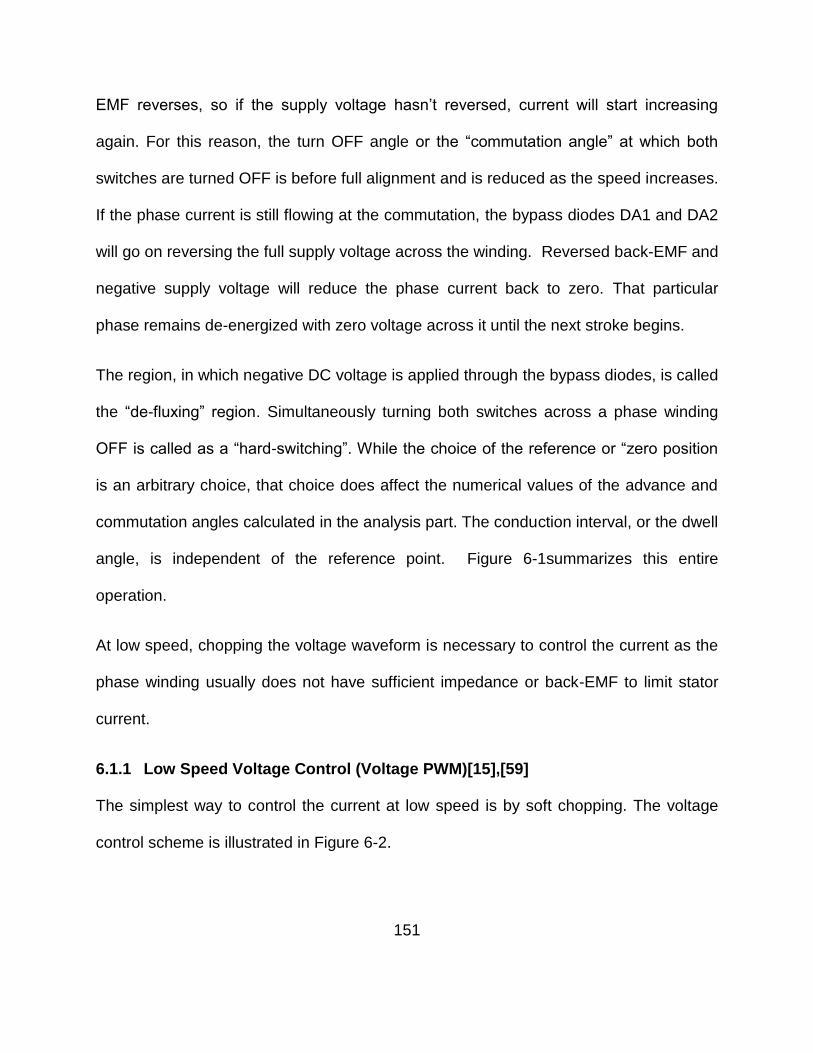
151

EMF reverses, so if the supply voltage hasn’t reversed, current will start increasing

again. For this reason, the turn OFF angle or the “commutation angle” at which both

switches are turned OFF is before full alignment and is reduced as the speed increases.

If the phase current is still flowing at the commutation, the bypass diodes DA1 and DA2

will go on reversing the full supply voltage across the winding. Reversed back-EMF and

negative supply voltage will reduce the phase current back to zero. That particular

phase remains de-energized with zero voltage across it until the next stroke begins.

The region, in which negative DC voltage is applied through the bypass diodes, is called

the “de-fluxing” region. Simultaneously turning both switches across a phase winding

OFF is called as a “hard-switching”. While the choice of the reference or “zero position

is an arbitrary choice, that choice does affect the numerical values of the advance and

commutation angles calculated in the analysis part. The conduction interval, or the dwell

angle, is independent of the reference point. Figure 6-1summarizes this entire

operation.

At low speed, chopping the voltage waveform is necessary to control the current as the

phase winding usually does not have sufficient impedance or back-EMF to limit stator

current.

6.1.1 Low Speed Voltage Control (Voltage PWM)[15],[59]

The simplest way to control the current at low speed is by soft chopping. The voltage

control scheme is illustrated in Figure 6-2.

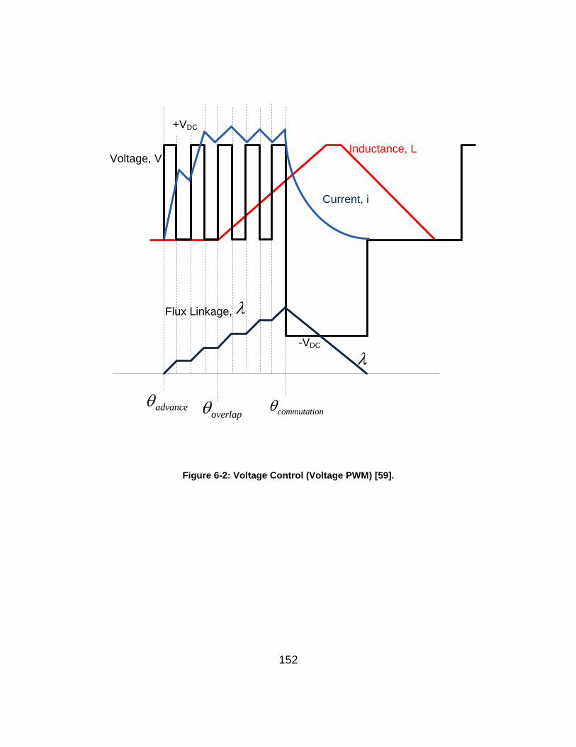
152

Inductance, LVoltage, V

+VDC

-VDC

Current, i

Flux Linkage,

advanceoverlap commutation

Figure 6-2: Voltage Control (Voltage PWM) [59].

153

In this scheme, one switch is left ON while the other switch is turned ON and OFF at a

higher frequency with a fixed duty cycle D = ONt

T . So instead of just controlling the

current during magnetic overlap, the duty cycle is kept constant during the entire fluxing

region (i.e. for entire dwell period). From the advance angle to the turn OFF angle, fixed

duty cycle voltage pulses are applied to the phase winding. During unaligned region,

the current increases rapidly. At the turn OFF angle, current is rapidly reduced by

turning OFF both the switches, and applying negative DC voltage through the bypass

diodes. Instead of soft chopping, hard chopping can also be used to control the current

magnitude during the fluxing region but it increases current ripple by a large factor. Soft

chopping produces lower acoustic noise, less EMI, and less DC ripple current in the

supply and reduces the filter capacitance requirement. In the voltage type control

strategy, turn on angle, turn off angle and duty cycle are the main control variables. As

speed increases, the duty cycle has to be increased to maintain the current. When this

duty cycle D becomes unity, the motor enters into a single pulse high speed operation

mode. During soft chopping, the average voltage applied to the phase winding is DVs.

6.1.2 Low Speed Current Control [15],[59]

Most traction drives are current controlled drives [60]. In this type of control strategy,

phase is magnetized using full supply voltage. Once the current approaches the set

point value, current is controlled around that value by hysteresis type of a control

scheme. After turn OFF angle, for de-fluxing, full negative voltage is applied by turning

both switches OFF. If the switching frequency is high and sufficient DC voltage is

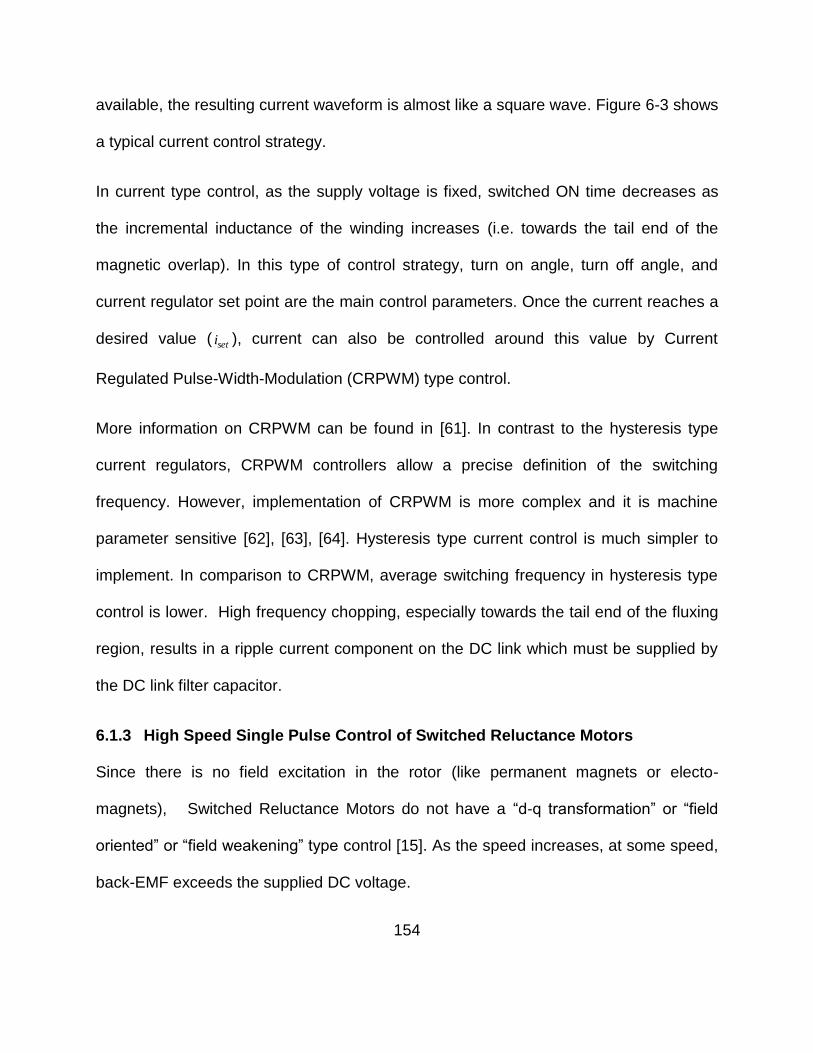
154

available, the resulting current waveform is almost like a square wave. Figure 6-3 shows

a typical current control strategy.

In current type control, as the supply voltage is fixed, switched ON time decreases as

the incremental inductance of the winding increases (i.e. towards the tail end of the

magnetic overlap). In this type of control strategy, turn on angle, turn off angle, and

current regulator set point are the main control parameters. Once the current reaches a

desired value ( seti ), current can also be controlled around this value by Current

Regulated Pulse-Width-Modulation (CRPWM) type control.

More information on CRPWM can be found in [61]. In contrast to the hysteresis type

current regulators, CRPWM controllers allow a precise definition of the switching

frequency. However, implementation of CRPWM is more complex and it is machine

parameter sensitive [62], [63], [64]. Hysteresis type current control is much simpler to

implement. In comparison to CRPWM, average switching frequency in hysteresis type

control is lower. High frequency chopping, especially towards the tail end of the fluxing

region, results in a ripple current component on the DC link which must be supplied by

the DC link filter capacitor.

6.1.3 High Speed Single Pulse Control of Switched Reluctance Motors

Since there is no field excitation in the rotor (like permanent magnets or electo-

magnets), Switched Reluctance Motors do not have a “d-q transformation” or “field

oriented” or “field weakening” type control [15]. As the speed increases, at some speed,

back-EMF exceeds the supplied DC voltage.

155

Figure 6-3: Current Type SRM Control.

0 0.01 0.02 0.03 0.04 0.05 0.06 0.07 0.08-800

-600

-400

-200

0

200

400

600

800

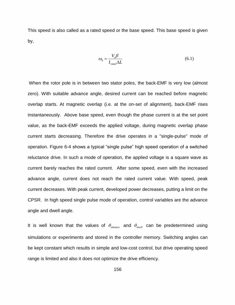
156

This speed is also called as a rated speed or the base speed. This base speed is given

by,

sb

rated

V

I L

(6.1)

When the rotor pole is in between two stator poles, the back-EMF is very low (almost

zero). With suitable advance angle, desired current can be reached before magnetic

overlap starts. At magnetic overlap (i.e. at the on-set of alignment), back-EMF rises

instantaneously. Above base speed, even though the phase current is at the set point

value, as the back-EMF exceeds the applied voltage, during magnetic overlap phase

current starts decreasing. Therefore the drive operates in a "single-pulse" mode of

operation. Figure 6-4 shows a typical “single pulse” high speed operation of a switched

reluctance drive. In such a mode of operation, the applied voltage is a square wave as

current barely reaches the rated current. After some speed, even with the increased

advance angle, current does not reach the rated current value. With speed, peak

current decreases. With peak current, developed power decreases, putting a limit on the

CPSR. In high speed single pulse mode of operation, control variables are the advance

angle and dwell angle.

It is well known that the values of advance and dwell can be predetermined using

simulations or experiments and stored in the controller memory. Switching angles can

be kept constant which results in simple and low-cost control, but drive operating speed

range is limited and also it does not optimize the drive efficiency.

157

Inductance, LVoltage, V

+VDC

-VDC

Current, i

advanceoverlap commutation

Figure 6-4: Single Pulse High Speed Operation of SRM Motors.

158

Turn-off angle can also be shifted synchronously with the turn-on angle (dwell angle can

be kept constant) while advance angle is changed. Other extreme in realizing traction

control is variation of all control variables i.e. advance angle, dwell angle and current set

point. Implementation becomes complex. Advance angle can also be calculated in real

time, which optimizes the output power and hence efficiency [65]. Large torque

oscillations can be observed when the advance angle is changed in increments [61] .

This can be avoided if the change is continuous (smaller).

Similar behavior can be observed during the change from one control strategy to

another, if a combination of strategies is used to optimize the drive efficiency and drive

operating area. Significant research has been done to estimate and optimize these

control parameters especially for below base speed operation [59],[15]. The following

section lists some of the control methods especially for high speed operation.

6.2 Literature Review – High Speed Single Pulse Control

Switched reluctance motors have three distinct regions of operation [47]. Below base

speed, current has to be controlled to the rated value or desired value using voltage

pulse width modulation or hysteresis band current control. Above base speed, applied

voltage is at the rated value and the current can only be controlled by adjusting advance

and dwell angle. In this region, the applied voltage is a square wave and resulting

current is a single pulse. When operated with the fixed voltage and fixed switching

angles, developed torque falls naturally as ω2. By increasing conduction angle in

159

proportion to speed, torque can be made to fall linearly in an inversely proportional way.

As the advance angle is increased, there comes a point where the current pulse

occupies half of the r . When the fluxing region exceeds 2r degrees, resultant

current never returns back to zero as the de-fluxing region becomes shorter than the

fluxing region. This case is similar to applying a DC voltage to a purely inductive circuit.

With each additional stroke, this causes continuous current build up. To avoid this, dwell

angle has to be limited to 50% of the stroke length. In the 3rd region of operation,

voltage is at the rated value and irrespective of the advance and the dwell angle the

current does not reach to the rated value. Current is still in single pulse mode and by

keeping advance and dwell angles fixed, the motor can be operated with its intrinsic

characteristics. Depending on the motor design, it is still possible to develop rated

power even though peak current is below the rated value. However, developed power

decreases rapidly and CPSR is limited.

When the rotor pole is in between two stator poles (unaligned region), 0dLd

.

Neglecting resistance R, we have,

di

v Ldt

(6.2)

Here uL L unaligned inductance which is constant is this case, and sv V (DC

supply voltage, with both switches ON). Therefore,

s u

diV L

dt (6.3)

160

And 0 0i i.e. current starts from zero at the beginning of the cycle and returns back

to zero. Rewriting the Equation (6.3), we get,

u

di Vs

dt L ,

s

u

Vi t t

L (6.4)

u set

s

L It

V

Therefore,

u set

s

L It

V ,

Hence the advance angle which guarantees that the required peak current Iset is

reached at the on-set of alignment is given by,

u setadv

s

L I

V (6.5)

Bose [65] and MacMinn [11] have used this formula to calculate the advance angle as

speed increases to produce the desired or rated power. This formula neglects the

winding resistance and assumes that the back-EMF is zero during the constant

inductance region (unaligned region). Since the advance angle has to be limited to the

161

unaligned region, we have 2adv unaligned r . This puts the limit on the highest

speed.

2r s

u set

V

L I

(6.6)

Equation (6.6) gives the maximum attainable speed considering limits on the

advancement angle to avoid continuous current. Ray et al. [66] used experiments to

calculate the advance angle required to get desired power as a function of speed and

load.

Bose et al. [65] used the speed control loop with the inner torque control loop for SRM

motors. Figure 6-5 illustrates this control strategy. In this control strategy, speed

feedback is compared with the speed command. Generated speed error is then

converted to the torque command through the PI controller. This torque command is

then converted to the peak current set point. The inner torque control loop is shown in

Figure 6-6. Using this current set point, along with the speed feedback and the DC

supply voltage feedback, advance angle or a turn ON angle is calculated based on the

Equation (6.5). Based on this advance angle, commutation angle or the turn OFF angle

is estimated from the predetermined values stored in the memory. Turn OFF angle is

first reduced linearly from the maximum allowable angle (which avoids braking torque)

to the half of that value. Above base speed turn off angle is kept constant. The

relationship between the torque, the phase current, and the firing angles is highly non-

linear and vary as functions of speed and load [67] , [15], [65].

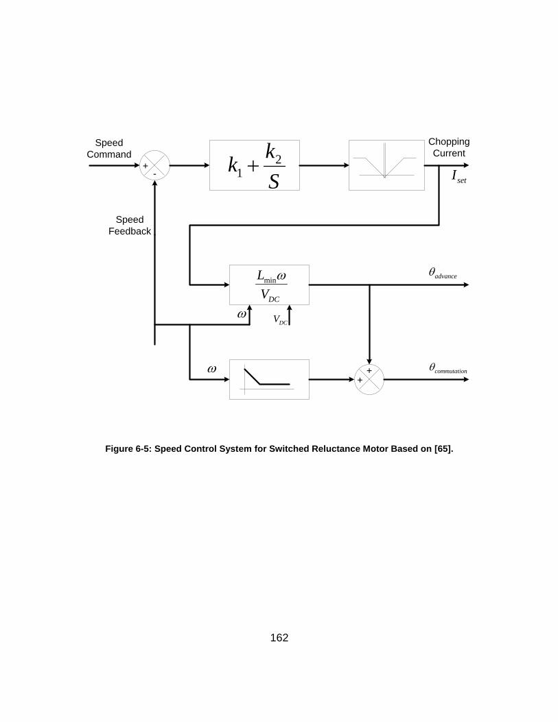
162

Speed

Command

Speed

Feedback

21

kk

S

Chopping

Current

setI+

-

++

min

DC

L

V

DCV

advance

commutation

Figure 6-5: Speed Control System for Switched Reluctance Motor Based on [65].

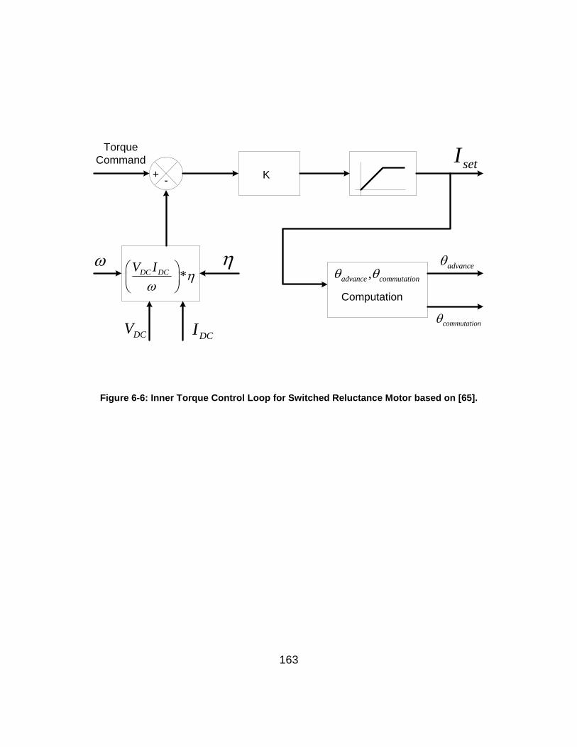
163

K

advance

commutation

,advance commutation

Computation

setI

DCVDCI

*DC DCV I

+-

Torque

Command

Figure 6-6: Inner Torque Control Loop for Switched Reluctance Motor based on [65].

164

If the converter efficiency is known, then based on the DC supply voltage, DC current,

and the speed feedback, torque can be roughly calculated as follows,

*DC DCe

V IT

(6.7)

According to [65], a high gain torque loop inside a speed control loop, linearizes the

overall control system. It enhances the speed response and also allows higher

controller gains within the stability limits for the speed loop. This method provides better

performance than the fixed angle type control strategies.

MacMinn et al.[12],[11] have proposed a closed loop control strategy for a very high

speed, starter-generator switched-reluctance aircraft engine. This control method is

shown in the Figure 6-7. This control method is very similar to Bose’s [65] method

except a phase current feedback is added and inner torque control loop is open. Since

the torque feedback is not always feasible. Figure 6-8 (taken from [11]) shows the

output torque as a function of current regulator set point ( setI). Using curve fitting,

various values of the current regulator set point as a function of desired output torque

can be calculated and stored in the controller memory. These values can be obtained

through simulations or through the experiments. Based on the torque requirement,

current regulator set point is estimated. Based on this current regulator set point, along

with the DC voltage and speed feedback, advance angle is calculated by using

Equation (6.5). Turn on angle (advance angle) is advanced such that the phase current

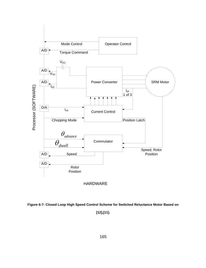
165

Operator Control

A/DTorque Command

Mode Control

Power Converter SRM Motor

Current Control

Iph

1 of 3

Position Latch

Commutator

Speed, Rotor

Position

Rotor

Position

A/D

A/D Speed

advance

dwell

Chopping Mode

D/AIref

VDC

A/D

A/DVDC

IDC

HARDWARE

Pro

ce

sso

r (S

OF

TW

AR

E)

Figure 6-7: Closed Loop High Speed Control Scheme for Switched Reluctance Motor Based on

[12],[11].

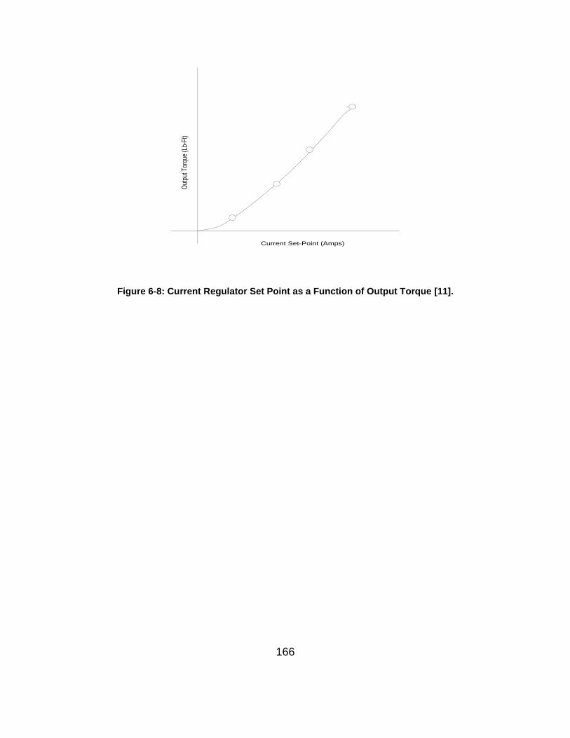
166

Current Set-Point (Amps)

Out

put T

orqu

e (L

b-Ft

)

Figure 6-8: Current Regulator Set Point as a Function of Output Torque [11].

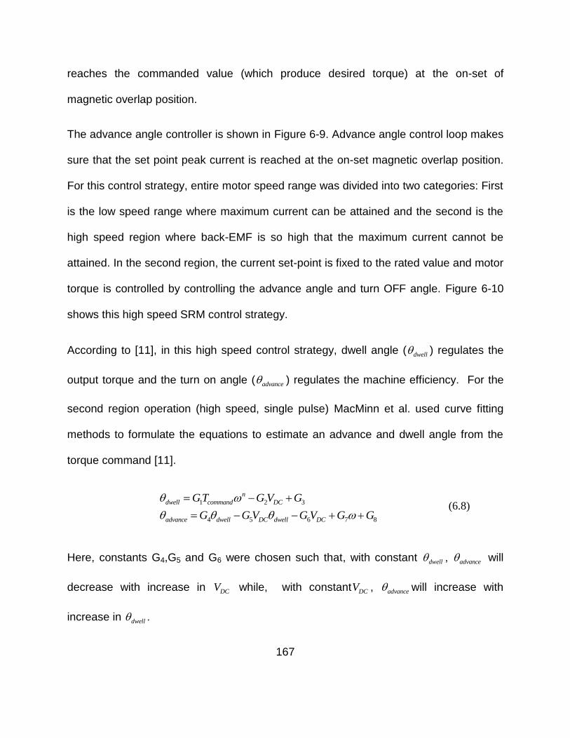
167

reaches the commanded value (which produce desired torque) at the on-set of

magnetic overlap position.

The advance angle controller is shown in Figure 6-9. Advance angle control loop makes

sure that the set point peak current is reached at the on-set magnetic overlap position.

For this control strategy, entire motor speed range was divided into two categories: First

is the low speed range where maximum current can be attained and the second is the

high speed region where back-EMF is so high that the maximum current cannot be

attained. In the second region, the current set-point is fixed to the rated value and motor

torque is controlled by controlling the advance angle and turn OFF angle. Figure 6-10

shows this high speed SRM control strategy.

According to [11], in this high speed control strategy, dwell angle ( dwell ) regulates the

output torque and the turn on angle ( advance ) regulates the machine efficiency. For the

second region operation (high speed, single pulse) MacMinn et al. used curve fitting

methods to formulate the equations to estimate an advance and dwell angle from the

torque command [11].

1 2 3

4 5 6 7 8

n

dwell command DC

advance dwell DC dwell DC

GT G V G

G G V G V G G

(6.8)

Here, constants G4,G5 and G6 were chosen such that, with constant dwell , advance will

decrease with increase in DCV while, with constant DCV , advance will increase with

increase in dwell .

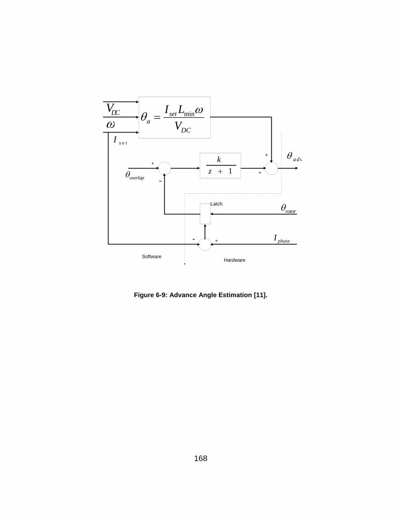
168

minseta

DC

I L

V

s e tI

DCV

1

k

z overlap

adv

phaseI

rotorLatch

SoftwareHardware

+

+

+

+

-

-

Figure 6-9: Advance Angle Estimation [11].

169

DWELL Angle Calculator

ADVANCE Angle Calculator

Dwell

Advance

Torque Command

DCV

setI fixed

Figure 6-10: High Speed SRM Control Based on [11].

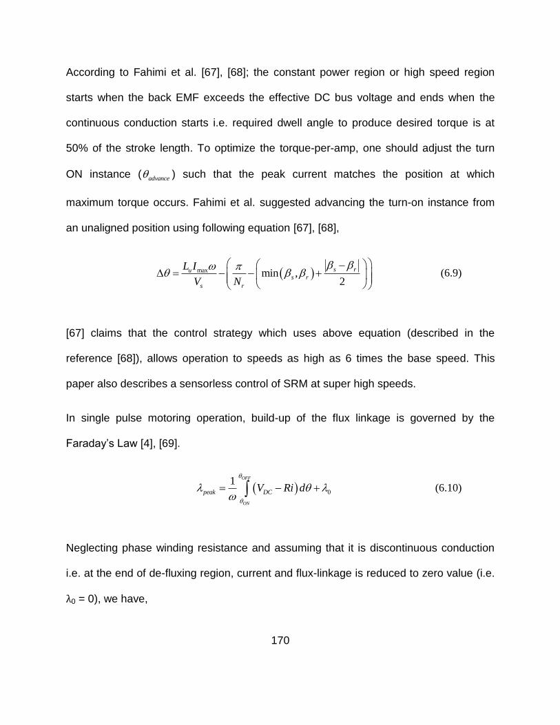
170

According to Fahimi et al. [67], [68]; the constant power region or high speed region

starts when the back EMF exceeds the effective DC bus voltage and ends when the

continuous conduction starts i.e. required dwell angle to produce desired torque is at

50% of the stroke length. To optimize the torque-per-amp, one should adjust the turn

ON instance ( advance ) such that the peak current matches the position at which

maximum torque occurs. Fahimi et al. suggested advancing the turn-on instance from

an unaligned position using following equation [67], [68],

max min ,2

s rus r

s r

L I

V N

(6.9)

[67] claims that the control strategy which uses above equation (described in the

reference [68]), allows operation to speeds as high as 6 times the base speed. This

paper also describes a sensorless control of SRM at super high speeds.

In single pulse motoring operation, build-up of the flux linkage is governed by the

Faraday’s Law [4], [69].

0

1 OFF

ON

peak DCV Ri d

(6.10)

Neglecting phase winding resistance and assuming that it is discontinuous conduction

i.e. at the end of de-fluxing region, current and flux-linkage is reduced to zero value (i.e.

λ0 = 0), we have,

171

DCpeak dwell

V

(6.11)

As the peak value of the flux-linkage decides the iron loss in the motor, dwell has to be

kept to the minimum [69]. Equation (6.5) guarantees that the peak current is reached at

the on-set of alignment. In unaligned inductance region, as the back-EMF is almost

zero, current rise is linear ( DC udi dt V L ). Current in the flat inductance region does not

contribute to the torque production whereas it increases the copper loss in the motor.

Moving the current closer the magnetic overlap position will reduce the copper loss but

to produce the same torque, the dwell has to be increased. Increased dwell increases

the peak value of the flux-linkage. Kioskeridis et al. [69], claim to have optimized the

turn ON and turn OFF angles for high speed single-pulse operation by finding the best

balance between copper loss and iron loss, i.e. between the minimum dwell and the

minimum advance angle. These values were determined using simulations and by

carrying out experiments. The SRM motor was rotated at a constant speed and at a

constant torque and the advance angle and the dwell angle was changed to find out the

best combination by measuring losses at each of those points. Kim et al. in [70],

describe a scheme for advance angle estimation for a single-pulse high speed

operation. To find out the turn ON angle which results in the maximum efficiency, 3D

characteristics of the estimated motor efficiency and torque as a function of the advance

and the commutation angle was investigated using extensive simulations. First for a

given speed, a set of combinations of the advance angle and the commutation angle

which produces same torque was calculated. From that set a combination which results

172

in maximum efficiency was then identified and recorded. According to [70] efficiency is

more sensitive to the advance angle than to the turn OFF angle.

All of the above mentioned SRM control strategies are of discontinuous type. Meaning,

at the beginning of the fluxing region (i.e. when the DC voltage is applied), phase

current starts from the zero and at the end of de-fluxing region (i.e. when the negative

DC supply voltage is applied), it returns back to the zero. Above base speed, back –

EMF, whose magnitude increases as the speed increases, exceeds the applied DC

voltage. Therefore the peak current decreases. With the peak current, co-energy area

decreases and hence the developed power reduces below the rated power. With

discontinuous type conduction, speeds as high as 6 times the base speed can be

achieved which means CPSR is limited to 6:1 [68].

According to Yahia [71], CPSR increases with the increase in the magnetic saliency

ratio i.e. the ratio of the aligned inductance to the unaligned inductance. CPSR and

output power also increases with the increase in the duration of inductance rise [71].

Morel [72] and Vujicic [73] lists the machine parameters that can be changed to

achieve wider constant power range.

Another way to increase the CPSR is by allowing continuous conduction. When the

conduction angle (dwell) is more than the half of the total cycle, current and flux-linkage

fail to return back to the zero as the de-fluxing region is less than the fluxing region. So

with each cycle, progressive growth of the current and the flux-linkage occurs resulting

in an unstable condition. Once the current has grown to the desired or rated value, it

173

can be controlled by keeping the fluxing region exactly equal to half of the cycle (i.e. one

stroke, in an 8/6 motor: 60°). If the de-fluxing region is maintained to the remaining half

of the stroke length, this growth can be sustained. This allows the motor to produce the

rated torque at much higher speeds.

Switched Reluctance Drives Limited has patents (US 5469039, US 5545964, US

5563488) on continuous conduction mainly for switched reluctance generators.

According to these patents, turn OFF angle is kept almost constant (it is decreased a

little bit as speed increases). Turn ON is initially changed such that it results in the

current growth from stroke to stroke. Once the desired peak current is reached, a

feedback control loop keeps the turn ON angle constant. If the load current is increased,

resultant error, through the PI controller causes the advance angle to increase. Since

turn OFF (or commutation) angle is constant, this increases fluxing region (dwell angle).

Resultant flux build-up causes increase in the peak current. Once the current rises

above new required set point, advance angle decreases back and stabilizes to a new

equilibrium point. As described in the next chapter, peak current set point can be used

to regulate the output power but for a given speed and the dwell angle, advance angle

can be changed to maximize the output power rather than to regulate the output power.

According to Korkosz et al. [74], by careful selection of control angles, with continuous

conduction, the rated power can be produced for a wide speed range. Although this

paper fails to elaborate the requirements on the dwell angle to initiate and maintain the

continuous conduction and the control method used/needed to stabilize the current

growth once continuous conduction is initiated. The paper provides the data from

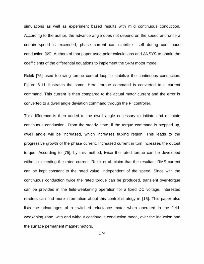
174

simulations as well as experiment based results with mild continuous conduction.

According to the author, the advance angle does not depend on the speed and once a

certain speed is exceeded, phase current can stabilize itself during continuous

conduction [69]. Authors of that paper used polar calculations and ANSYS to obtain the

coefficients of the differential equations to implement the SRM motor model.

Rekik [75] used following torque control loop to stabilize the continuous conduction.

Figure 6-11 illustrates the same. Here, torque command is converted to a current

command. This current is then compared to the actual motor current and the error is

converted to a dwell angle deviation command through the PI controller.

This difference is then added to the dwell angle necessary to initiate and maintain

continuous conduction From the steady state, if the torque command is stepped up,

dwell angle will be increased, which increases fluxing region. This leads to the

progressive growth of the phase current. Increased current in turn increases the output

torque. According to [75], by this method, twice the rated torque can be developed

without exceeding the rated current. Rekik et al. claim that the resultant RMS current

can be kept constant to the rated value, independent of the speed. Since with the

continuous conduction twice the rated torque can be produced, transient over-torque

can be provided in the field-weakening operation for a fixed DC voltage. Interested

readers can find more information about this control strategy in [16]. This paper also

lists the advantages of a switched reluctance motor when operated in the field-

weakening zone, with and without continuous conduction mode, over the induction and

the surface permanent magnet motors.

175

Torque to

Current +

-PI +

+ Power

ConverterSRM

refTrefI

feedbackI

Errordwell

50%dwell

Figure 6-11: Closed Loop Torque Control Loop for Continuous Conduction Based on [75].

Long et. al. [76] and Rekik et al. [75], suggested that for a machine operating with

conventional discontinuous current, extended speed operation can be achieved by

reducing the number of turns per pole, but this reduces torque-per-amp at or below the

base speed. At extended speeds, reducing the number of turns per pole reduces the

effective the back EMF. It allows an improvement in the power capability within the DC

link voltage constraint. According to Long et al., continuous phase current excitation

enhances the extended power capability at extended speeds without significantly

compromising the system or machine efficiencies [76]. Machines with continuous

current can be designed with more number of turns per pole to increase the torque-per-

am at or below base speed. This reduces the inverter current rating and hence silicon

requirement [76].

In continuous conduction, phase current starts from a non-zero value and grows with

every stroke. As described earlier, this phenomenon can be controlled. In SRDL

patents, as described earlier, growing phase current is controlled to the desired value,

176

by changing the advance angle with turn OFF angle almost fixed. In the references [75]

and [16], phase current is controlled by changing the dwell angle while the advance

angle is just used to maximize the efficiency. In both of these continuous conduction

type control methods, dwell angle is changed (50% +) to regulate the output power.

Literature available on these two continuous conduction type control schemes does not

give any details on what is the continuous conduction, how it is initiated, how the current

growth is stabilized, what is the relationship between developed output power and

control / machine parameters, what happens to the average current and what are the

key parameters. The primary goal of this research was to answer these questions. Next

chapter describes the analysis of continuous conduction using linear magnetic model.

177

7 CONTINUOUS CONDUCTION ANALYSIS AND SIMULATION RESULTS

The continuous conduction type control scheme discussed here is very similar to that

typically used to control low speed operation (i.e. discontinuous conduction mode type

control). The relevant control quantities are the advance angle, the dwell angle and the

current regulator set point. It is shown that the dwell angle is the key factor and must be

sufficiently large to sustain the continuous conduction, but excessive values are shown

to reduce the motor efficiency. Advance angle is then set at an “optimum” value that

maximizes energy conversion and control of the developed power is achieved by

raising/lowering the peak current regulator set point. This control results in the

developed power that is directly proportional to the motor current magnitude, achieving

good efficiency at partial as well as full load conditions. Dynamic response can be

sluggish when the dwell is set at the minimum value necessary to support the

continuous conduction for steady state operation. A sophisticated controller that will

widen the dwell during transient intervals in order to improve speed of response and

then collapse the dwell to minimum requirement during steady speed operation can

resolve this potential problem. The remainder of this chapter is organized in six

sections. Section 7.1 contains a description of the parameters of an example SRM

motor intended for a 26:1 CPSR application that is used as an illustration throughout the

chapter. This section also reviews the linear model theory predicting an infinite CPSR

for the SRM operating in continuous conduction. If the speed sensitive losses are

178

ignored, linear magnetic model predicts that the CPSR of the SRM motor can be infinite

when the continuous conduction type high speed control scheme is used [13]. A linear

magnetic model does not provide accurate results for analyzing low speed performance,

but it has been shown to be accurate in predicting high-speed performance of switched

reluctance motor in continuous as well as discontinuous conduction mode [13]. Section

7.2 describes different simulation models of the example motor. Section 7.3 provides

the simulation results for the continuous conduction type control scheme. Section 7.4

and 7.5 describe the mathematical analysis of the example motor when continuous

conduction type control scheme is used for the operation of the SRM motor in the

constant power region. This mathematical analysis tries to answer some of the

questions like how SRM goes into the continuous conduction, how the current growth is

contained, which control and machine design parameters affect the output power and

resultant average current, what happens to the average current and some insight into

the continuous conduction based SRM controller. For verification purpose, the

simulation results have been compared with the analytical results.

7.1 Example Motor Model

Data for the example motor was obtained by using a program [77] designed by the Oak

Ridge National Laboratory. The motor is a four phase 8/6 SRM design. Flux linkage

data obtained from the design program for one phase is displayed in the Figure 7-1, and

Figure 7-2. The data has been displayed for one pole pitch which is 60o for an 8/6

machine. The flux linkage data for this phase would repeat itself in each 60o interval.

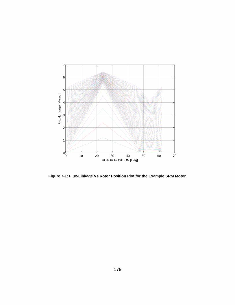
179

Figure 7-1: Flux-Linkage Vs Rotor Position Plot for the Example SRM Motor.

0 10 20 30 40 50 60 700

1

2

3

4

5

6

7

ROTOR POSITION [Deg]

Flu

x-L

inkage [

V-s

ec]

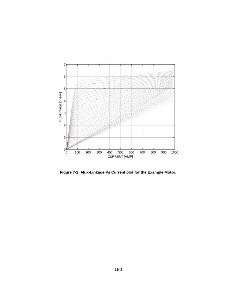
180

Figure 7-2: Flux-Linkage Vs Current plot for the Example Motor.

0 100 200 300 400 500 600 700 800 900 10000

1

2

3

4

5

6

7

CURRENT [AMP]

Flu

x-L

inkage [

V-s

ec]

181

Flux linkage data for the other three phases can be generated by delaying the data in

Figure 7-3 by 150, 300 and 45o. Flux linkages values dependent on both the rotor

position and the winding current. In Figure 7-1, the flux linkages are plotted versus rotor

position, in one degree increments, with winding current as a parameter. The winding

current varies from 0 to 983.607 amps in the steps of 16.394 amperes. The peak of the

flux linkage curves occurs at 22.5o which is the “completely aligned” position while the

minimum flux linkage occurs at 52.5o which is the “completely unaligned” position. In

this position the rotor pole is exactly in between two adjacent stator poles. The “zero

degree” position has been chosen corresponding to the condition where the rotor and

stator poles are “point-to-point” i.e. at the onset of alignment or the on-set of

magnetic/physical overlap. In Figure 7-2 data is displayed with the rotor position as

parameter. Rotor position is varied from 0° to 60° in the steps of 1°. In Figure 7-3,

saturation can be observed for the currents greater than 300A during magnetic overlap.

7.1.1 Nomenclature and Parameters of the Example Motor

bN = Base Speed (250 RPM), R = Winding Resistance Per Phase (0.014 Ω), pI = Peak Current

(650 A), rmsI = Rated RMS Current (450 A), rP = Rated Power (320 HP),CPSR = 26 (Top Speed

6500 RPM), aL = inductance in aligned position (73.38mH), uL = inductance in the unaligned

position (4.15mH), a uL L L = (69.23mH), = pole arc (22.5°), r = pole pitch (60),

adv = advance angle, sV = DC supply voltage (700 V).

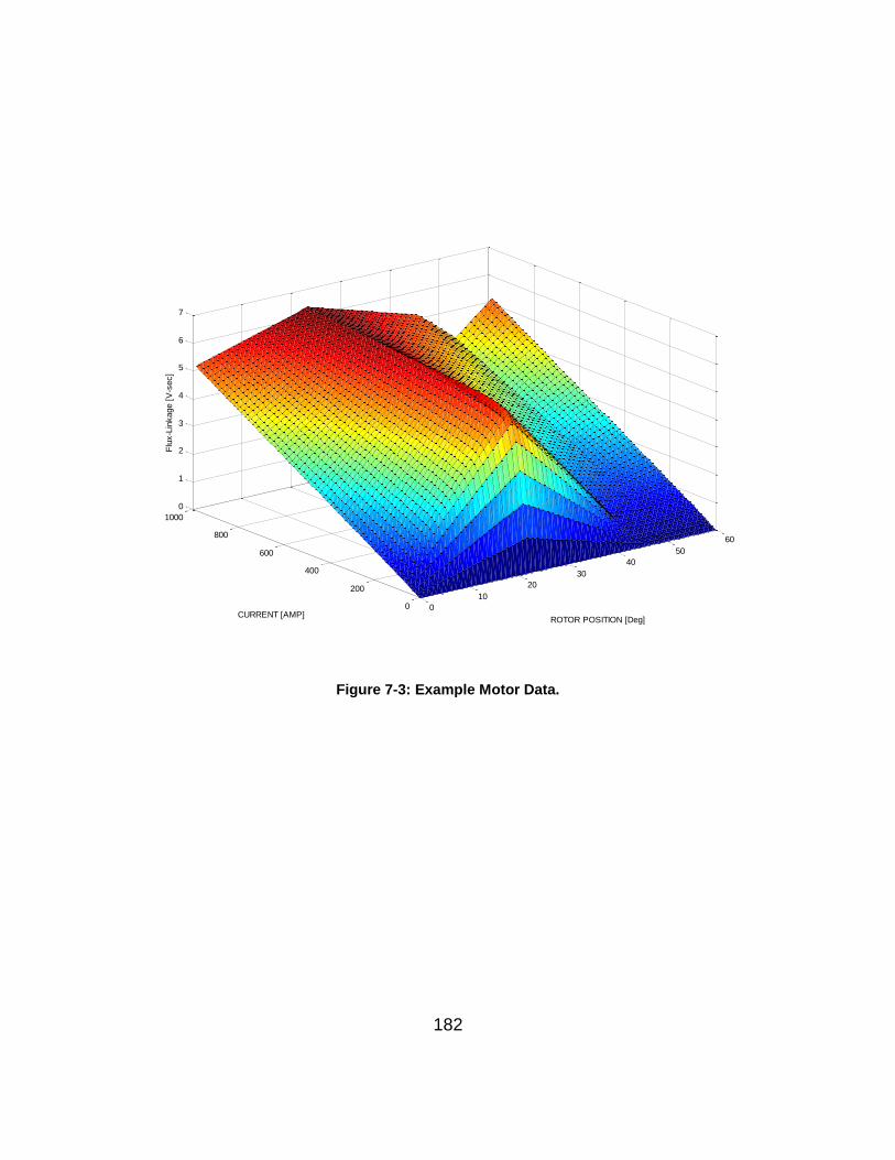
182

Figure 7-3: Example Motor Data.

0

10

20

30

40

50

60

0

200

400

600

800

1000

0

1

2

3

4

5

6

7

ROTOR POSITION [Deg]CURRENT [AMP]

Flu

x-L

inkage [

V-s

ec]

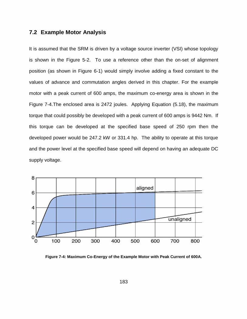
183

7.2 Example Motor Analysis

It is assumed that the SRM is driven by a voltage source inverter (VSI) whose topology

is shown in the Figure 5-2. To use a reference other than the on-set of alignment

position (as shown in Figure 6-1) would simply involve adding a fixed constant to the

values of advance and commutation angles derived in this chapter. For the example

motor with a peak current of 600 amps, the maximum co-energy area is shown in the

Figure 7-4.The enclosed area is 2472 joules. Applying Equation (5.18), the maximum

torque that could possibly be developed with a peak current of 600 amps is 9442 Nm. If

this torque can be developed at the specified base speed of 250 rpm then the

developed power would be 247.2 kW or 331.4 hp. The ability to operate at this torque

and the power level at the specified base speed will depend on having an adequate DC

supply voltage.

Figure 7-4: Maximum Co-Energy of the Example Motor with Peak Current of 600A.

184

7.2.1 Linear Model

For flux-linkages, we have,

, , *i l i i (7.1)

Ignoring saturation we have,

*L i (7.2)

For linear mode it is assumed that the flux-linkages only depend on the rotor position

and not the current level. Another way to determine the flux-linkages is,

sV iR dt (7.3)

Using above equations for flux-linkages, the motor current can be calculated by the

following equation.

sV iR dt

iL

(7.4)

So based on the DC supply voltage information, along with per phase winding

resistance and per phase winding inductance information, it is possible to estimate the

phase current. For a linear model which ignores saturation, per phase inductance

information can be obtained by dividing the flux linkage data in Figure 7-3 by the

185

corresponding current. The linear inductance profile for the example model over one

pole pitch is shown in the Figure 7-5. This graph was obtained by obtained by the

division of the flux-linkage data by the corresponding current (16.393 A). Note that the

inductance during the unaligned region is not perfectly flat. An idealized linear

inductance profile having a constant inductance in the unaligned zone was developed

using Matlab and Simulink to carry out the continuous conduction analysis and

simulations for high-speed operation. First part of the Figure 7-6 shows this flat

unaligned inductance profile while second part shows non-flat (similar to the actual

example motor profile) unaligned inductance profile. Figure 7-7 shows the Simulink

based linear model which uses this linear per phase inductance profile.

7.2.2 Nonlinear Model

Considering current dependent saturation, phase current can be estimated as follows,

,

sV iR dti

L i

(7.5)

Here per phase inductance profile not only depends on the rotor position, it also

depends on the phase current. Inductance profile needed for the above equation can be

obtained by dividing the flux-linkage data of Figure 7-3 by the current for a fixed rotor

angle. Figure 7-8 shows this resultant per phase inductance profile which incorporates

the current dependence. Figure 7-9 shows the Simulink based non-linear model

developed to carry out simulations for comparison with the linear model at high speed.

186

Figure 7-5: Linear Magnetic Model of the Example Motor.

187

Figure 7-6: Linear Inductance Profile of the Example Motor.

0 10 20 30 40 50 600

0.01

0.02

0.03

0.04

0.05

0.06

0.07

0.08

ROTOR POSITION [deg]

IND

UC

TA

NC

E [

mH

]

Lu = 4.15mH

On-Set of Alignment

La = 73.38 mH

0 10 20 30 40 50 600

0.01

0.02

0.03

0.04

0.05

0.06

0.07

0.08

ROTOR POSITION [deg]

IND

UC

TA

NC

E [

mH

]

188

Figure 7-7: Simulink Model for the Example Motor [ L(θ) ].

waveforms

speed 1

3750

rad2deg

-K-

rad /sec 2 RPM 1

-K-

psi / L

omega

-C-

inductance

0.04107

d Theta

z-1

z

d L

z-1

z

cycles2

floor

cycles1

39

current

angle

-C-

Zero Volts 1

0

Zero Volts

0

Voltage Values

voltage .mat

Vdc

-700

Torque Values

torque .mat

Theta (Deg )1

Switch 3

Switch 2

Switch 1

Subtract

Saturation 1

Rs

-K-

Rounding

Function

ceil

Product 3

Product 2

Product

Omega 1

392 .7

Math

Function

|u|2

Lookup Table

Logical

Operator 1

NOT

Logical

Operator

AND

Integrator

1

s

Instant Torque

Inductance Values

L.mat

Inductance

Fluxing

Flux Linkage Vs Current

Flux Linkage Values

flux .mat

Flux Linkage

Divide 2

Divide 1

Current Values

current .mat

Current Controller

Constant

1/2

Compare

To Constant

>= 0

Clock1

60

-C-

-Vdc

-Vs

+Vdc1

Vs

Current

Current

Current

Current

Current

Flux Linkage

Flux Linkage

Flux Linkage

Inductance

Inductance

Vdc

Vdc

omega

Theta rad

Theta radTheta

Theta Deg.

189

Figure 7-8: Inductance Profile of the Example SRM.

0 10 20 30 40 50 600

0.01

0.02

0.03

0.04

0.05

0.06

0.07

0.08

Rotor Position (Deg)

Inducta

nce (

H)

Inductance Vs. Rotor Position

Increasing Current

190

Figure 7-9: Simulink Model for the Example Motor Simulation [ L(θ,i) ].

waveforms

speed

rad2deg

-K-

rad /sec 2 RPM

-K-

psi / L

omega

-C-

inductance comparison

inductance

d psi

z-1

z

d Theta

z-1

z

d L

z-1

z

cycles2

floor

cycles

current 1

current

co energy

back EMF

angle

-C-

Zero Volts 1

0

Zero Volts

0

Voltage Values

voltage .mat

Vdc

Torque Values

torque .matTheta (Deg )

Switch 3

Switch 2

Switch 1

Subtract

Saturation

Rs

-K-

Rounding

Function

ceil

Rotor Position

Product 4

Product 3

Product 2

Product 1

Product

Omega

Math

Function

|u|2

Lookup

Table (n-D)2

2-D T (u)u1

u2

Lookup

Table (n-D)1

2-D T (u)u1

u2

Logical

Operator 1

NOT

Logical

Operator

AND

Integrator

1

s

Instant Torque

Inductance Values

L.mat

Inductance

Fluxing

Flux Linkage Vs Current

Flux Linkage Values

flux .mat

Flux Linkage

Divide 3

Divide 2

Divide 1

Current Values

current .mat

Current Controller

Constant 2

17

Constant

1/2

Compare

To Constant

>= 0

Clock1

60

-C-

-Vdc

-Vs

+Vdc1

Vs

Current

Current

Current

Current

Current

Current

Current

Flux Linkage

Flux Linkage

Flux Linkage

Flux Linkage

Vdc

Vdc

Inductance

Inductance

omega

omega

Theta rad

Theta rad Theta

Theta

Theta Deg.

Theta Deg.

back EMF

I 2

I 2

191

7.2.3 Nonlinear Model with Partial Derivatives

From Equation (5.3) applied voltage can be given by the following equation,

( , ) ( , )

. .s

i di iV iR

i dt

(7.6)

This equation can be modified to the following form to estimate the phase current,

1 ( , )

.( , ) s

di iV iR

idt

i

(7.7)

The partial derivatives required in above equation to calculate phase current can be

derived from the example motor data shown in the Figure 7-3. Interested readers can

refer to [51] , [15], and [4] for more information on various mathematical methods those

can be used to manipulate the flux-linkage data ,i to obtain the partial derivatives

tan

,

i cons t

i

and

tan

,

cons t

i

i

.

Figure 7-10 shows these partial derivatives obtained using Matlab. Figure 7-11 shows

the Simulink based motor model which uses these partial derivatives and Equation (7.7)

to estimate the phase current. During the analysis, this model was not used.

7.2.4 Nonlinear Model with Current Estimation from Flux-Linkage Data

By using piecewise cubic spline interpolation (Matlab command interp1), it is possible to

manipulate the flux-linkage data λ(θ,i), in the Figure 7-3, to estimate the phase current

as a function of the flux-linkage and the rotor position i.e. i(λ,θ).

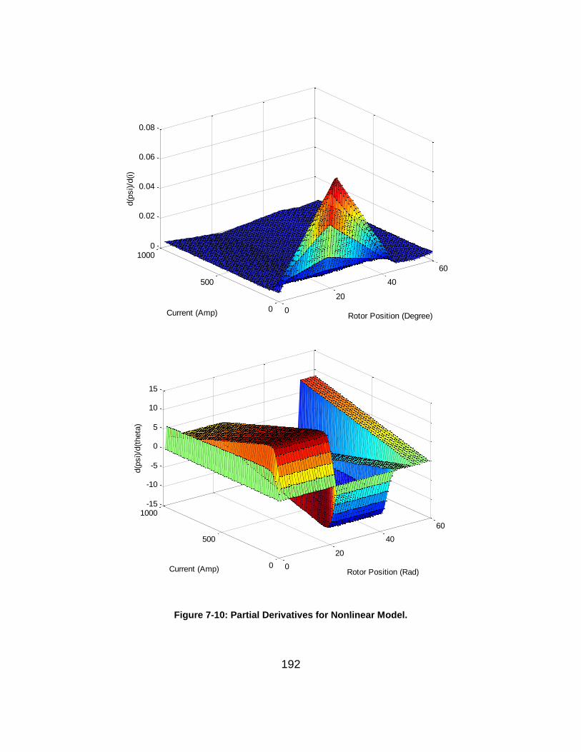
192

Figure 7-10: Partial Derivatives for Nonlinear Model.

0

20

40

60

0

500

10000

0.02

0.04

0.06

0.08

Rotor Position (Degree)Current (Amp)

d(p

si)/d

(i)

0

20

40

60

0

500

1000-15

-10

-5

0

5

10

15

Rotor Position (Rad)Current (Amp)

d(p

si)/d

(theta

)

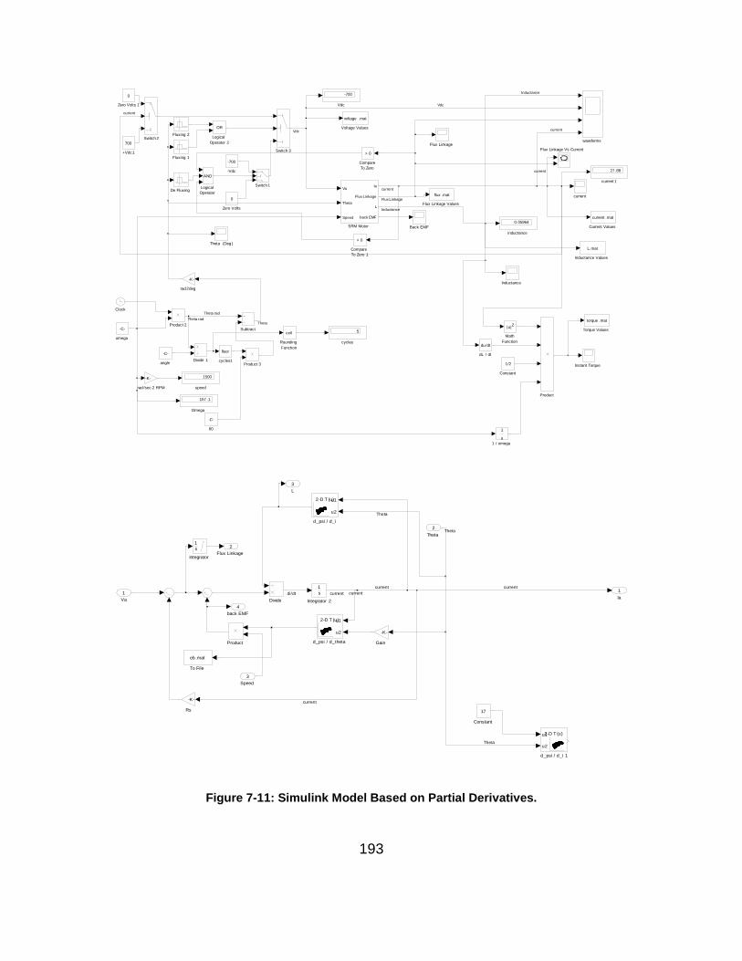
193

Figure 7-11: Simulink Model Based on Partial Derivatives.

waveforms

speed

1500

rad2deg

-K-

rad /sec 2 RPM

-K-

omega

-C-

inductance

0.05964

dL / dt

du /dt

cycles1

floor

cycles

5

current 1

27 .88

current

angle

-C-

Zero Volts 1

0

Zero Volts

0

Voltage Values

voltage .mat

Vdc

-700

Torque Values

torque .mat

Theta (Deg )

Switch 3

Switch 2

Switch 1

Subtract

SRM Motor

Va

Theta

Speed

Ia

Flux Linkage

L

back EMF

Rounding

Function

ceil

Product 3

Product 2

Product

Omega

157 .1

Math

Function

|u|2

Logical

Operator 2

OR

Logical

Operator

AND

Instant Torque

Inductance Values

L.mat

Inductance

Fluxing 2

Fluxing 1

Flux Linkage Vs Current

Flux Linkage Values

flux .mat

Flux Linkage

Divide 1

De Fluxing

Current Values

current .mat

Constant

1/2

Compare

To Zero 1

> 0

Compare

To Zero

> 0

Clock

Back EMF

60

-C-

1 / omega

1

u

-Vdc

-700

+Vdc1

700

current

current

current

current

Inductance

Inductance

Vdc

Vdc

Theta rad

Theta radTheta

Flux Linkage

back EMF

4

L

3

Flux Linkage

2

Ia

1

d_psi / d_theta

2-D T (u)u1

u2

To File

eb .mat

Rs

-K-

Product

Integrator 2

1

s

Integrator

1

s

Gain

-K-

Divide

Constant

17

d_psi / d_i 1

2-D T (u)u1

u2

d_psi / d_i

2-D T (u)u1

u2

Speed

3

Theta

2

Va

1 di/dt

current

current

current

currentcurrent

Theta

Theta

Theta

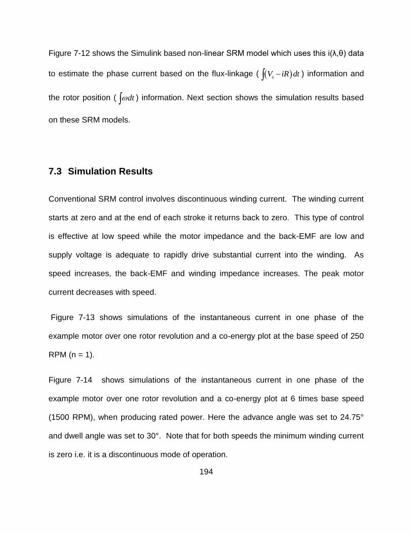
194

Figure 7-12 shows the Simulink based non-linear SRM model which uses this i(λ,θ) data

to estimate the phase current based on the flux-linkage ( sV iR dt ) information and

the rotor position ( dt ) information. Next section shows the simulation results based

on these SRM models.

7.3 Simulation Results

Conventional SRM control involves discontinuous winding current. The winding current

starts at zero and at the end of each stroke it returns back to zero. This type of control

is effective at low speed while the motor impedance and the back-EMF are low and

supply voltage is adequate to rapidly drive substantial current into the winding. As

speed increases, the back-EMF and winding impedance increases. The peak motor

current decreases with speed.

Figure 7-13 shows simulations of the instantaneous current in one phase of the

example motor over one rotor revolution and a co-energy plot at the base speed of 250

RPM (n = 1).

Figure 7-14 shows simulations of the instantaneous current in one phase of the

example motor over one rotor revolution and a co-energy plot at 6 times base speed

(1500 RPM), when producing rated power. Here the advance angle was set to 24.75°

and dwell angle was set to 30°. Note that for both speeds the minimum winding current

is zero i.e. it is a discontinuous mode of operation.

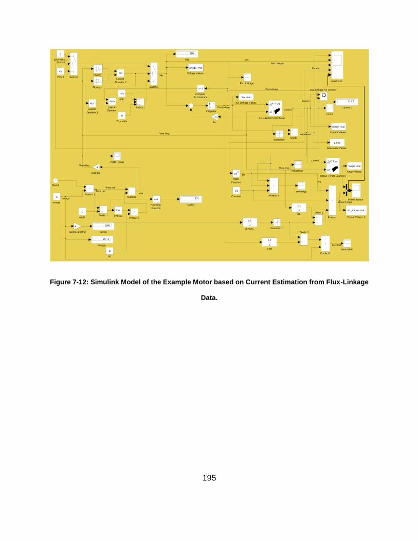
195

Figure 7-12: Simulink Model of the Example Motor based on Current Estimation from Flux-Linkage

Data.

waveforms

speed

1500

rad2deg

-K-

rad /sec 2 RPM

-K-

omega

-C-

d psi

z-1

z

d Theta

z-1

z

d L

z-1

z

cycles2

floor

cycles

13

current 1

211.3

current (psi,theta )

2-D T (u)u1

u2current

co energy

back EMF

angle

-C-

Zero Volts 1

0

Zero Volts

0

Voltage Values

voltage .mat

Vdc

700

Torque Values 1

lin _torque .mat

Torque Values

torque .mat

Torque (Theta ,Current )

2-D T (u)u1

u2

Theta (Deg )

Switch 3

Switch 2

Switch 1

Subtract

Saturation 1

Saturation

Rs

-K-

Rounding

Function

ceil

Product 4

Product 3

Product 2

Product 1

Product

Omega

157 .1

Math

Function

|u|2

Logical

Operator 2

OR

Logical

Operator 1

NOT

Logical

Operator

AND

Integrator

1

s

Instant Torque

Inductance Values

L.mat

Inductance

Fluxing 1

Fluxing

Flux Linkage Vs Current

Flux Linkage Values

flux .mat

Flux Linkage

Divide 3

Divide 2

Divide 1

Divide

Current Values

current .mat

Constant

1/2

Compare

To Constant

>= 0

Clock1

60

-C-

-Vdc

-Vs

+Vdc1

Vs

Current

Current

Current

Current

Current

Current

Flux Linkage

Flux Linkage

Flux Linkage

Vdc

Vdc

omega

Theta rad

Theta radTheta

Theta Deg.

Theta Deg.

Theta Deg.

Inductance

back EMF

I 2

I 2

Linear Torque

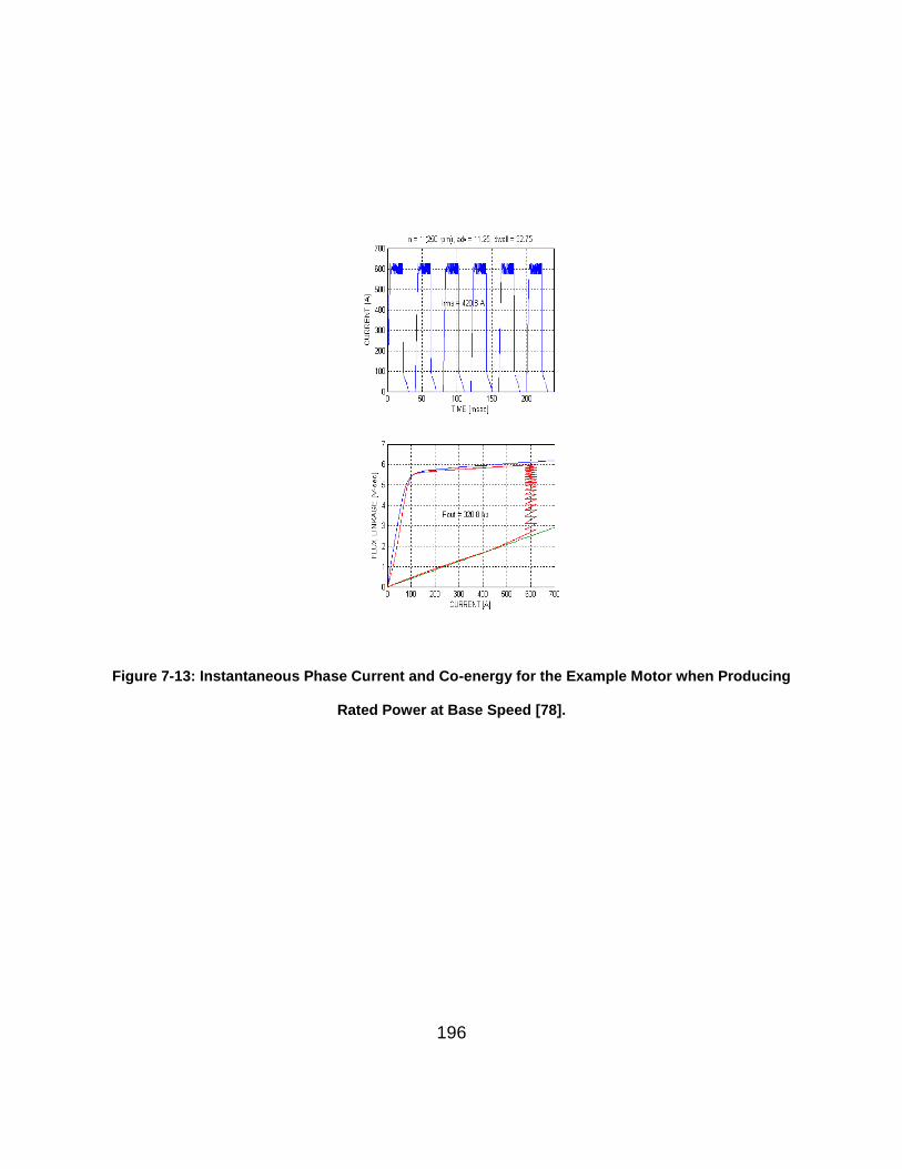
196

Figure 7-13: Instantaneous Phase Current and Co-energy for the Example Motor when Producing

Rated Power at Base Speed [78].

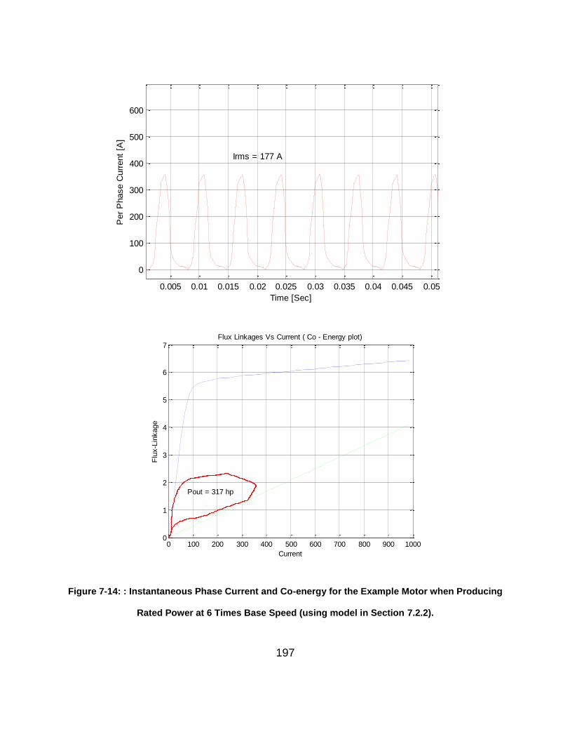
197

Figure 7-14: : Instantaneous Phase Current and Co-energy for the Example Motor when Producing

Rated Power at 6 Times Base Speed (using model in Section 7.2.2).

0.005 0.01 0.015 0.02 0.025 0.03 0.035 0.04 0.045 0.05

0

100

200

300

400

500

600P

er

Phase C

urr

ent

[A]

Time [Sec]

Irms = 177 A

0 100 200 300 400 500 600 700 800 900 10000

1

2

3

4

5

6

7

Flu

x-L

inkage

Current

Flux Linkages Vs Current ( Co - Energy plot)

Pout = 317 hp

198

Unfortunately the co-energy decreases faster than the reciprocal of speed and therefore

the CPSR is finite when the SRM is controlled using discontinuous type control scheme.

In case of the example motor, as Figure 7-13 indicates, the CPSR is 6:1. That is the

relative speed of 6 is the highest speed at which rated power (320 hp) can be

developed. At speeds above 1500 rpm, developed power will be less than 320 hp.

In continuous conduction, the minimum winding current is greater than zero. By

selecting a dwell angle more than 50% of the stroke length or the rotor pole pitch r

(30o for the 8/6 example motor), the fluxing region (or the magnetizing region) is kept

more than the de-fluxing (or the de-magnetizing) region. That is, if the dwell is 31°, de-

fluxing region will be r dwell = 60° - 31° = 29°. At the end of each stroke, flux returns

to a higher value than the start value. At the end of each stroke, residual value of the

flux linkage and hence the minimum current increases. Peak current also increases with

each stroke. Once the desired peak current (current regulator set point) is reached,

current regulator will impose a short zero volt-sec interval (in this case 31° - 29° = 2°) in

the fluxing region by turning OFF one of the switches. By doing so, it will make both the

fluxing region and the de-fluxing region of equal width. During periodic steady state, with

continuous conduction, it is necessary that there be a precise positive and negative volt-

second applied to the winding during each stroke such that the winding current starts

and returns to the same minimum value at the end of each stroke. So during steady

state, both fluxing region and de-fluxing region will be of the same width (in this case

29°) guarantying desired peak current during each stroke.

199

Figure 7-15 and Figure 7-16 shows the example motor operating at the desired top

speed of 6500 rpm for discontinuous and continuous conduction respectively. In both

cases the set point of the peak current regulator is 600A, and the advance angle is

22.5o. The two cases differ slightly in dwell angle. In the discontinuous conduction

case the dwell is 30o which is not adequate to trigger continuous conduction; while in

the continuous conduction case the dwell angle is one degree wider at 31o.

Figure 7-15 shows that when operating with discontinuous conduction, at 6500 RPM

small current is driven into the motor. The RMS current is about 33A, and the developed

power is about 60hp which is far less than the 320hp rating. With continuous

conduction, RMS current is about 333A which is within the 425A rating and the

developed power is about 670hp, which is more than twice the rated power developed

with the rated current at the specified base speed. Note that the current regulator

operates one time during each stroke (during fluxing region) to limit the peak current to

the 600A value (current regulator set-point). The current regulator kicks in because the

dwell is slightly greater than 50% of the stroke length. Figure 7-17 illustrates how

continuous conduction is started and how it is stabilized. The co-energy plot in the

Figure 7-16 justifies the use of a linear inductance model to predict SRM performance

during continuous conduction at high speed. When the winding current is large (600A in

this case), the rotor is in the vicinity of the unaligned position where magnetic saturation

is not a factor. When the rotor is in the vicinity of the aligned position where magnetic

saturation is generally a factor, the winding current is at the minimum value, which is too

low to involve the nonlinearity or saturation.

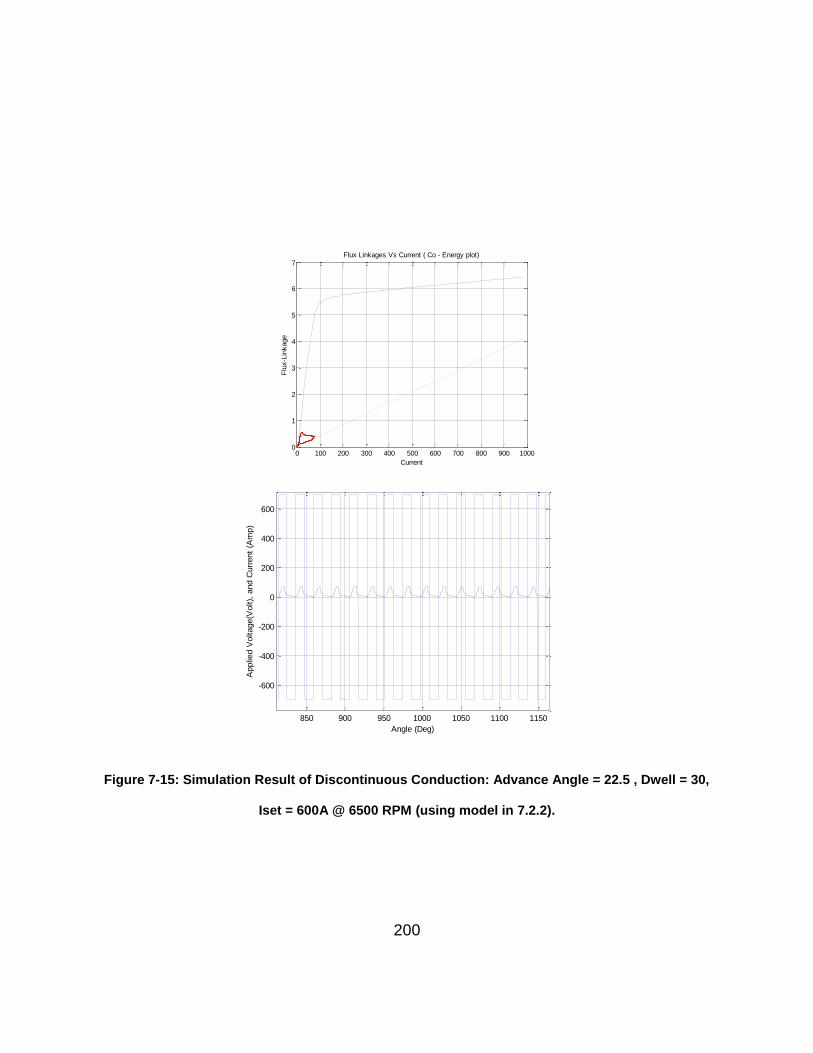
200

Figure 7-15: Simulation Result of Discontinuous Conduction: Advance Angle = 22.5 , Dwell = 30,

Iset = 600A @ 6500 RPM (using model in 7.2.2).

0 100 200 300 400 500 600 700 800 900 10000

1

2

3

4

5

6

7

Flu

x-L

inkage

Current

Flux Linkages Vs Current ( Co - Energy plot)

850 900 950 1000 1050 1100 1150

-600

-400

-200

0

200

400

600

Angle (Deg)

Applied V

oltage(V

olt),

and C

urr

ent

(Am

p)

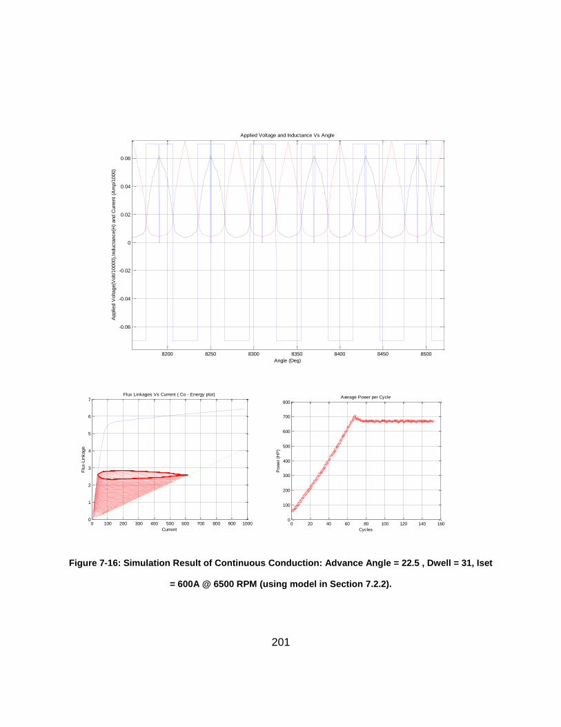
201

Figure 7-16: Simulation Result of Continuous Conduction: Advance Angle = 22.5 , Dwell = 31, Iset

= 600A @ 6500 RPM (using model in Section 7.2.2).

8200 8250 8300 8350 8400 8450 8500

-0.06

-0.04

-0.02

0

0.02

0.04

0.06

Angle (Deg)

Applie

d V

oltage(V

olt/1

0000),

Inducta

nce(H

) and C

urr

ent

(Am

p/1

000)

Applied Voltage and Inductance Vs Angle

0 100 200 300 400 500 600 700 800 900 10000

1

2

3

4

5

6

7

Flu

x-L

inkage

Current

Flux Linkages Vs Current ( Co - Energy plot)

0 20 40 60 80 100 120 140 1600

100

200

300

400

500

600

700

800

Cycles

Pow

er

(HP

)

Average Power per Cycle

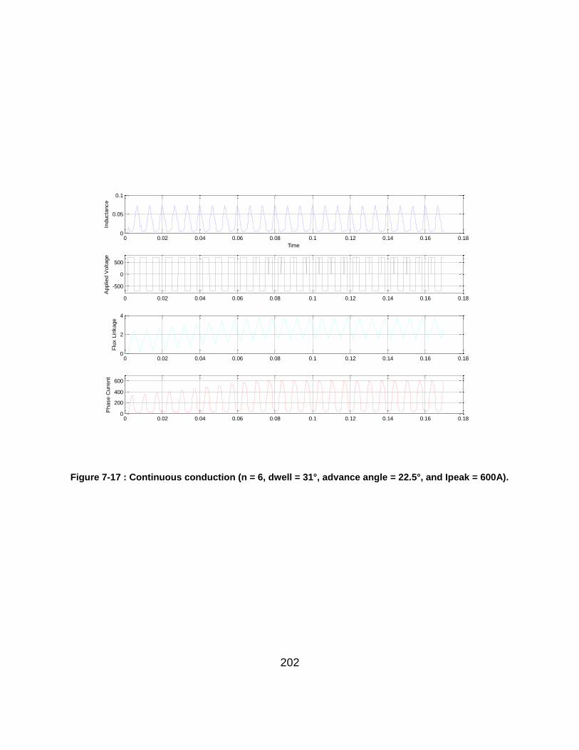
202

Figure 7-17 : Continuous conduction (n = 6, dwell = 31°, advance angle = 22.5°, and Ipeak = 600A).

0 0.02 0.04 0.06 0.08 0.1 0.12 0.14 0.16 0.180

0.05

0.1

Inducta

nce

Time

0 0.02 0.04 0.06 0.08 0.1 0.12 0.14 0.16 0.18

-500

0

500

Applie

d V

oltage

0 0.02 0.04 0.06 0.08 0.1 0.12 0.14 0.16 0.180

2

4

Flu

x L

inkage

0 0.02 0.04 0.06 0.08 0.1 0.12 0.14 0.16 0.180

200

400

600

Phase C

urr

ent

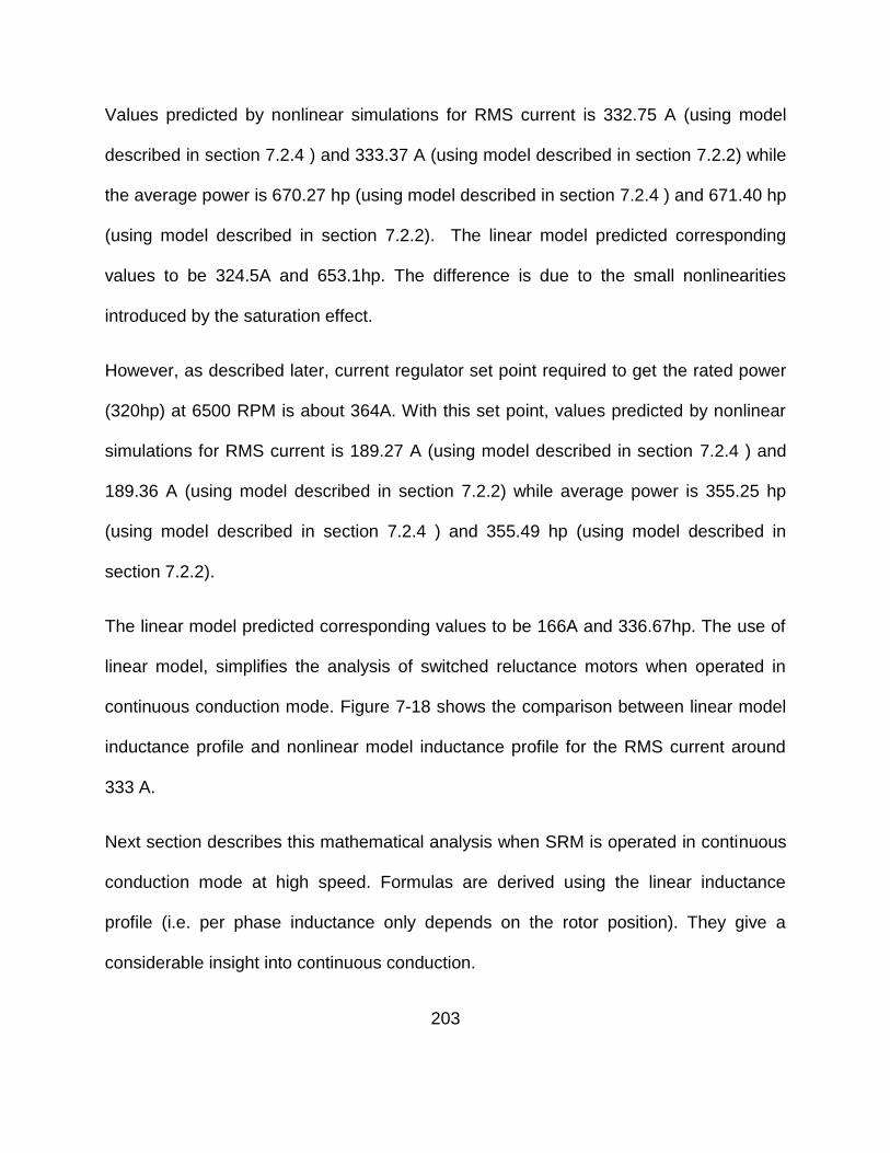
203

Values predicted by nonlinear simulations for RMS current is 332.75 A (using model

described in section 7.2.4 ) and 333.37 A (using model described in section 7.2.2) while

the average power is 670.27 hp (using model described in section 7.2.4 ) and 671.40 hp

(using model described in section 7.2.2). The linear model predicted corresponding

values to be 324.5A and 653.1hp. The difference is due to the small nonlinearities

introduced by the saturation effect.

However, as described later, current regulator set point required to get the rated power

(320hp) at 6500 RPM is about 364A. With this set point, values predicted by nonlinear

simulations for RMS current is 189.27 A (using model described in section 7.2.4 ) and

189.36 A (using model described in section 7.2.2) while average power is 355.25 hp

(using model described in section 7.2.4 ) and 355.49 hp (using model described in

section 7.2.2).

The linear model predicted corresponding values to be 166A and 336.67hp. The use of

linear model, simplifies the analysis of switched reluctance motors when operated in

continuous conduction mode. Figure 7-18 shows the comparison between linear model

inductance profile and nonlinear model inductance profile for the RMS current around

333 A.

Next section describes this mathematical analysis when SRM is operated in continuous

conduction mode at high speed. Formulas are derived using the linear inductance

profile (i.e. per phase inductance only depends on the rotor position). They give a

considerable insight into continuous conduction.

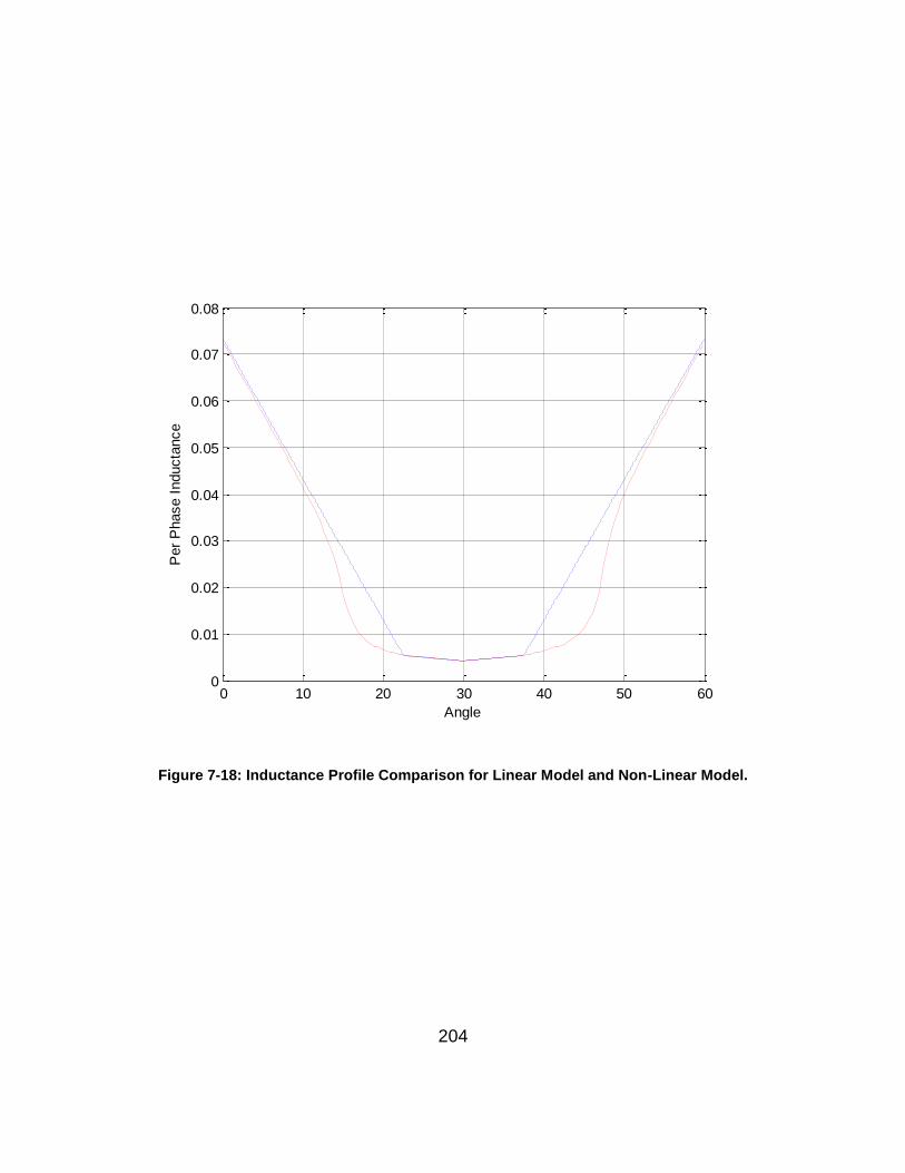
204

Figure 7-18: Inductance Profile Comparison for Linear Model and Non-Linear Model.

0 10 20 30 40 50 600

0.01

0.02

0.03

0.04

0.05

0.06

0.07

0.08

Per

Phase I

nducta

nce

Angle

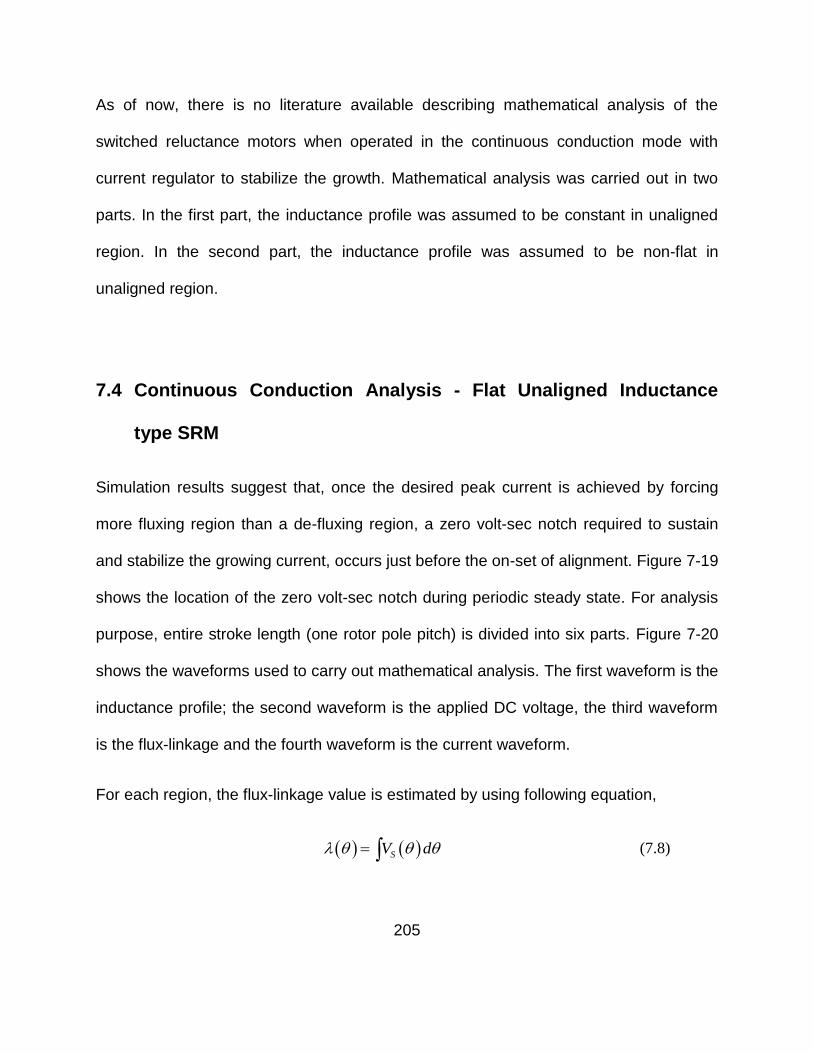
205

As of now, there is no literature available describing mathematical analysis of the

switched reluctance motors when operated in the continuous conduction mode with

current regulator to stabilize the growth. Mathematical analysis was carried out in two

parts. In the first part, the inductance profile was assumed to be constant in unaligned

region. In the second part, the inductance profile was assumed to be non-flat in

unaligned region.

7.4 Continuous Conduction Analysis - Flat Unaligned Inductance

type SRM

Simulation results suggest that, once the desired peak current is achieved by forcing

more fluxing region than a de-fluxing region, a zero volt-sec notch required to sustain

and stabilize the growing current, occurs just before the on-set of alignment. Figure 7-19

shows the location of the zero volt-sec notch during periodic steady state. For analysis

purpose, entire stroke length (one rotor pole pitch) is divided into six parts. Figure 7-20

shows the waveforms used to carry out mathematical analysis. The first waveform is the

inductance profile; the second waveform is the applied DC voltage, the third waveform

is the flux-linkage and the fourth waveform is the current waveform.

For each region, the flux-linkage value is estimated by using following equation,

SV d (7.8)

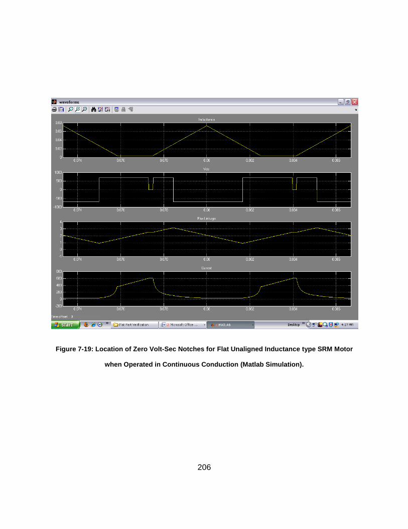
206

Figure 7-19: Location of Zero Volt-Sec Notches for Flat Unaligned Inductance type SRM Motor

when Operated in Continuous Conduction (Matlab Simulation).

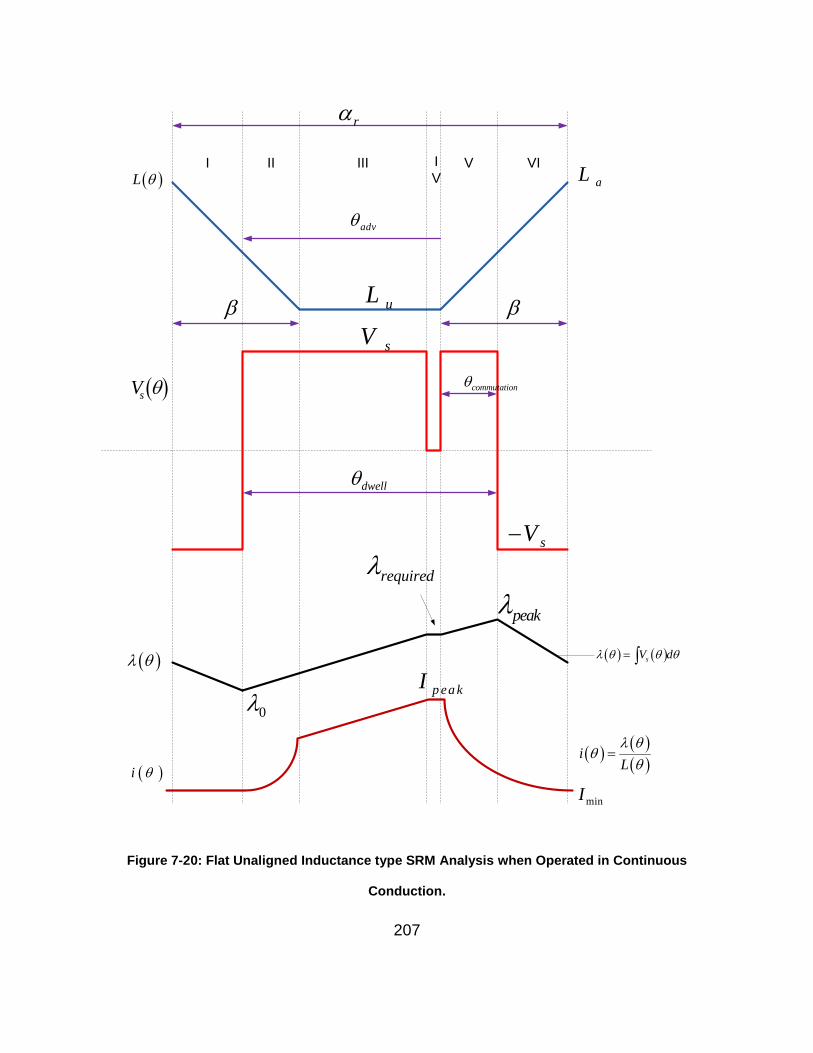
207

required

0

I II III I

VV VI

adv

r

commutation

dwell

L

sV

i

iL

sV d

aL

uL

sV

sV

peak

p ea kI

minI

Figure 7-20: Flat Unaligned Inductance type SRM Analysis when Operated in Continuous

Conduction.

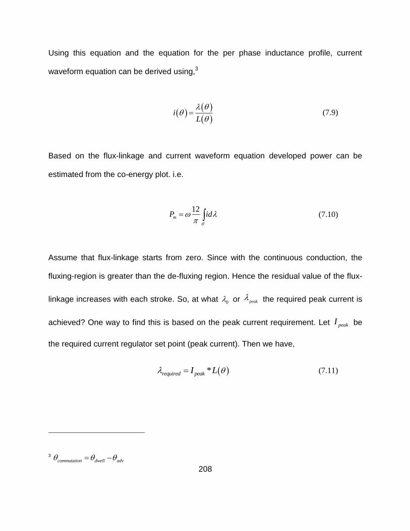
208

Using this equation and the equation for the per phase inductance profile, current

waveform equation can be derived using,3

iL

(7.9)

Based on the flux-linkage and current waveform equation developed power can be

estimated from the co-energy plot. i.e.

12

mP id

(7.10)

Assume that flux-linkage starts from zero. Since with the continuous conduction, the

fluxing-region is greater than the de-fluxing region. Hence the residual value of the flux-

linkage increases with each stroke. So, at what 0 or peak the required peak current is

achieved? One way to find this is based on the peak current requirement. Let peakI be

the required current regulator set point (peak current). Then we have,

*required peakI L (7.11)

3 commutation dwell adv

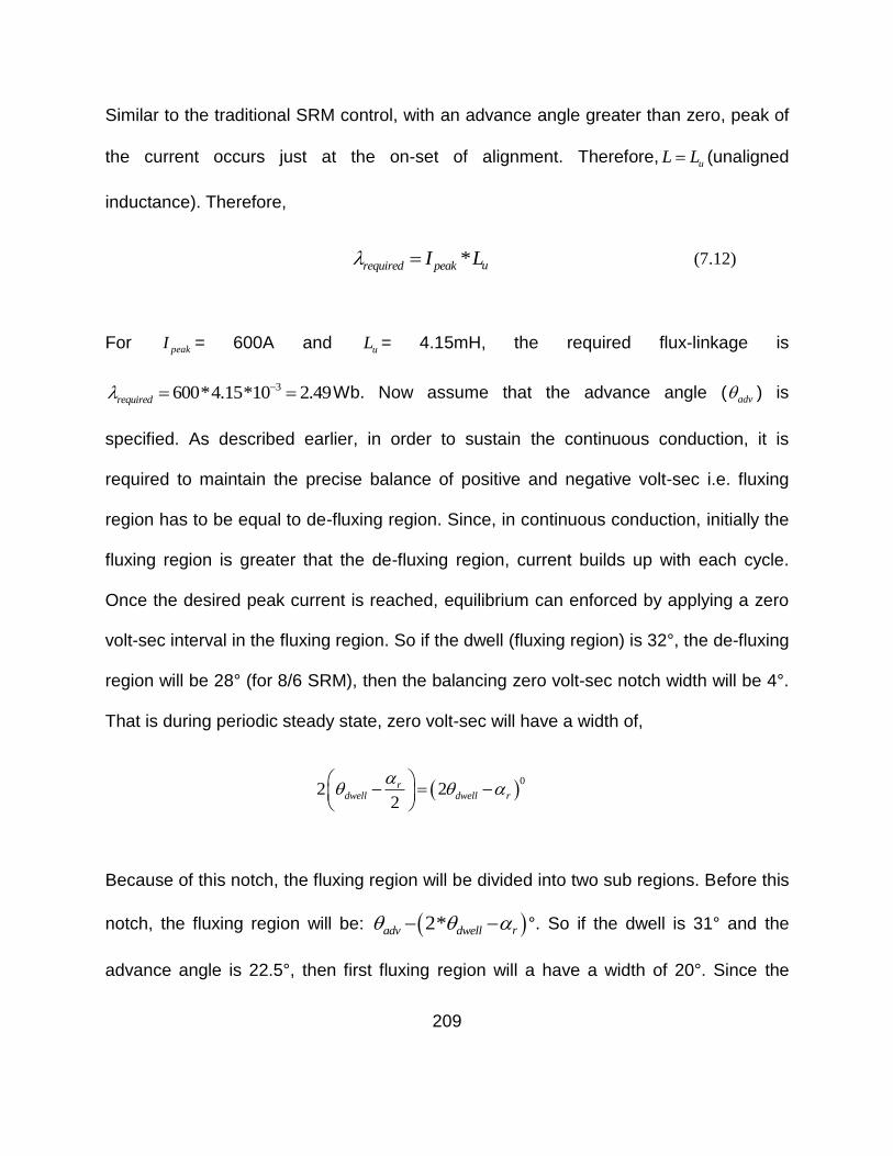
209

Similar to the traditional SRM control, with an advance angle greater than zero, peak of

the current occurs just at the on-set of alignment. Therefore, uL L (unaligned

inductance). Therefore,

* urequired peakI L (7.12)

For peakI = 600A and uL = 4.15mH, the required flux-linkage is

3600*4.15*10 2.49required Wb. Now assume that the advance angle ( adv ) is

specified. As described earlier, in order to sustain the continuous conduction, it is

required to maintain the precise balance of positive and negative volt-sec i.e. fluxing

region has to be equal to de-fluxing region. Since, in continuous conduction, initially the

fluxing region is greater that the de-fluxing region, current builds up with each cycle.

Once the desired peak current is reached, equilibrium can enforced by applying a zero

volt-sec interval in the fluxing region. So if the dwell (fluxing region) is 32°, the de-fluxing

region will be 28° (for 8/6 SRM), then the balancing zero volt-sec notch width will be 4°.

That is during periodic steady state, zero volt-sec will have a width of,

0

2 22

rdwell dwell r

Because of this notch, the fluxing region will be divided into two sub regions. Before this

notch, the fluxing region will be: 2* radv dwell °. So if the dwell is 31° and the

advance angle is 22.5°, then first fluxing region will a have a width of 20°. Since the

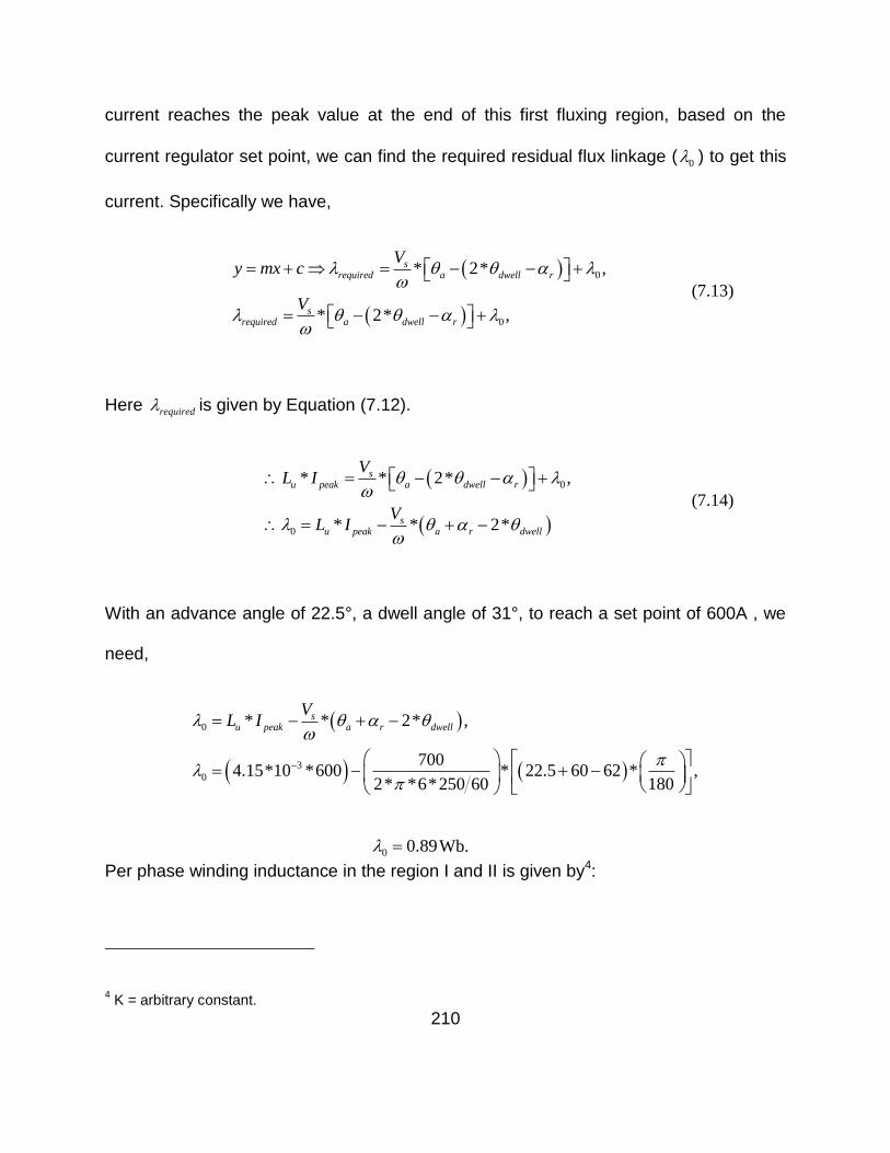
210

current reaches the peak value at the end of this first fluxing region, based on the

current regulator set point, we can find the required residual flux linkage ( 0 ) to get this

current. Specifically we have,

0

0

* 2* ,

* 2* ,

srequired a dwell r

srequired a dwell r

Vy mx c

V

(7.13)

Here required is given by Equation (7.12).

0

0

* * 2* ,

* * 2*

su peak a dwell r

su peak a r dwell

VL I

VL I

(7.14)

With an advance angle of 22.5°, a dwell angle of 31°, to reach a set point of 600A , we

need,

0

3

0

* * 2* ,

7004.15*10 *600 * 22.5 60 62 * ,

2* *6*250 60 180

su peak a r dwell

VL I

0 0.89 Wb.

Per phase winding inductance in the region I and II is given by4:

4 K = arbitrary constant.

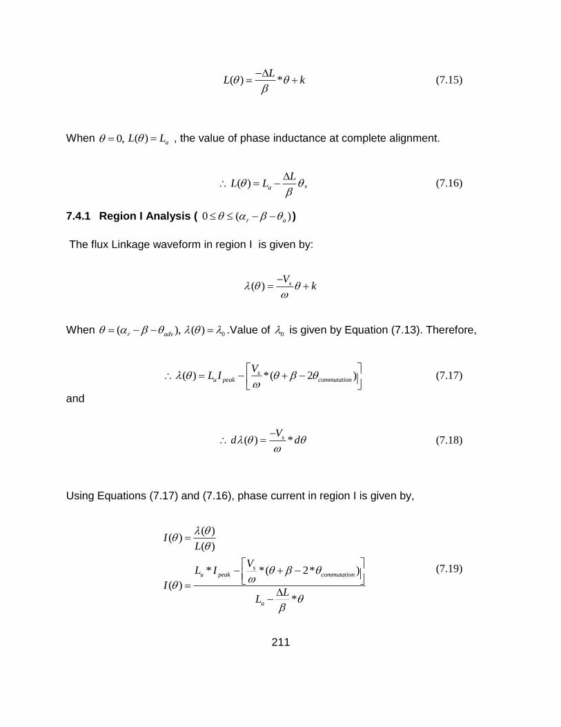
211

( ) *L

L k

(7.15)

When 0, ( ) aL L , the value of phase inductance at complete alignment.

( ) ,a

LL L

(7.16)

7.4.1 Region I Analysis ( 0 ( )r a )

The flux Linkage waveform in region I is given by:

( ) sVk

When ( ),r adv 0( ) .Value of 0 is given by Equation (7.13). Therefore,

( ) *( 2 )su peak commutation

VL I

(7.17)

and

( ) *sVd d

(7.18)

Using Equations (7.17) and (7.16), phase current in region I is given by,

( )( )

( )

* *( 2* )

( )

*

su peak commutation

a

IL

VL I

IL

L

(7.19)

212

Using this current and Equation (7.18) in (5.18), power produced in the region I is given

by,

( ) ( )

0 0

( ) ( )* ( ) ( )* ( )r a r a

P di i d

( )

1

0

( )

1

0

( )

1

0

( )* ( )

* *( 2* )

* *

*

* *( 2* )

* *

*

r a

r a

r a

su peak commutation

s

a

su peak commutation

s

a

P i d

VL I

VP d

LL

VL I

VP d

LL

2

1

2

( )ln ( )

( )2* ln

a r as u peak s

r a

a

a r as

commutation a

a

LV L I VLPL L

LL

LV LL

L LL

L

(7.20)

Details of this and other mathematical calculations are attached in the Appendix 0.

Flux-linkage in region II and III can be calculated as follows:

( ) sVk

When ( ),r a 0( ) .The value of 0 is given in Equation(7.13).

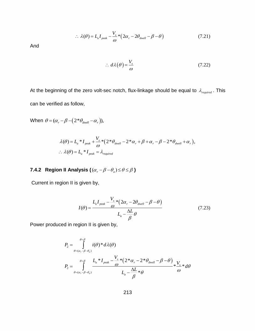
213

( ) * 2 2su peak r dwell

VL I

(7.21)

And

sVd

(7.22)

At the beginning of the zero volt-sec notch, flux-linkage should be equal to required . This

can be verified as follow,

When ( 2* ),r dwell r

( ) * * 2* 2* 2* ,

( ) *

su peak dwell r r dwell r

u peak required

VL I

L I

7.4.2 Region II Analysis ( ( )r a )

Current in region II is given by,

* 2 2

( )

su peak r dwell

a

VL I

IL

L

(7.23)

Power produced in region II is given by,

2

( )

2

( )

( )* ( )

* * 2* 2*

* *

*

r a

r a

su peak r dwell

s

a

P i d

VL I

VP d

LL

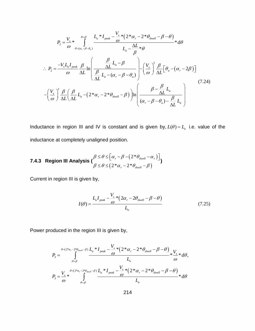
214

2

( )

* * 2* 2*

* *

*r a

su peak r dwell

s

a

VL I

VP d

LL

2

2

2

ln 2

( )

2* 2* ln

( )

as u peak s

a r

a r a

as

a r dwell

r a a

LV L I VLPL L

LL

LV LL

L LL

L

(7.24)

Inductance in region III and IV is constant and is given by, ( ) uL L i.e. value of the

inductance at completely unaligned position.

7.4.3 Region III Analysis (

2*

2* 2*

r dwell r

r dwell

)

Current in region III is given by,

* 2 2

( )

su peak r dwell

u

VL I

IL

(7.25)

Power produced in the region III is given by,

2* 2*

3

2* 2*

3

* * 2* 2*

* * ,

* * 2* 2*

* *

r dwell

r dwell

su peak r dwell

s

u

su peak r dwell

s

u

VL I

VP d

L

VL I

VP d

L

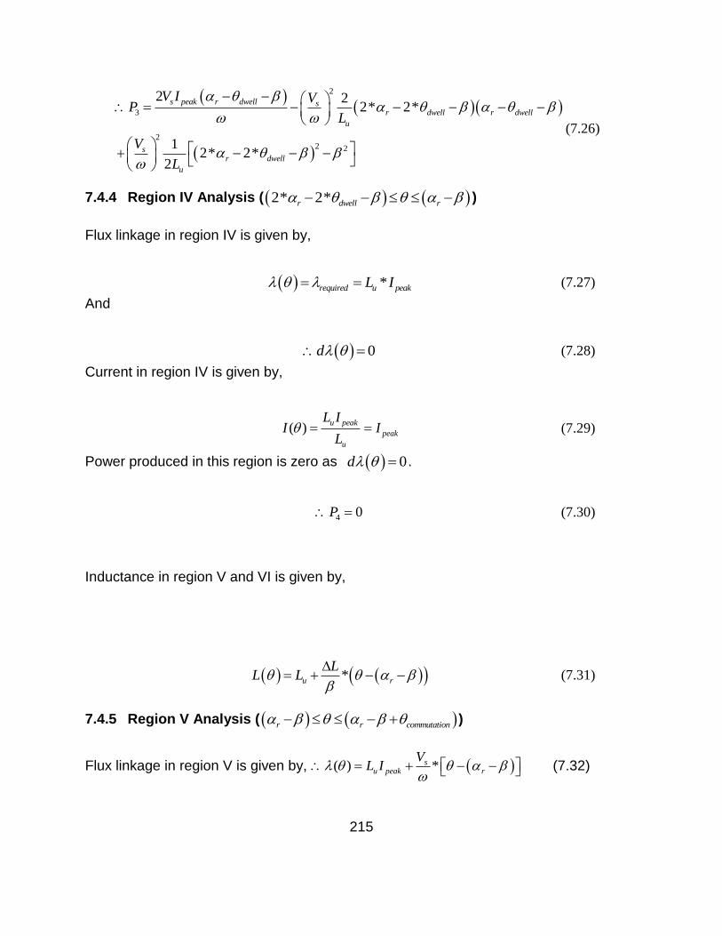
215

2

3

22 2

2 22* 2*

12* 2*

2

s peak r dwell sr dwell r dwell

u

sr dwell

u

V I VP

L

V

L

(7.26)

7.4.4 Region IV Analysis ( 2* 2*r dwell r )

Flux linkage in region IV is given by,

*required u peakL I (7.27)

And

0d (7.28)

Current in region IV is given by,

( )u peak

peak

u

L II I

L (7.29)

Power produced in this region is zero as 0d .

4 0P (7.30)

Inductance in region V and VI is given by,

*u r

LL L

(7.31)

7.4.5 Region V Analysis ( r r commutation )

Flux linkage in region V is given by, ( ) *su peak r

VL I

(7.32)

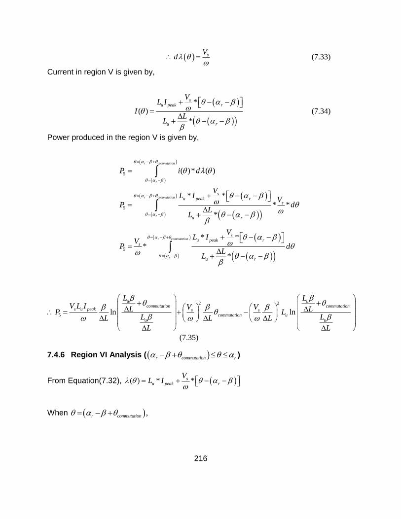
216

sVd

(7.33)

Current in region V is given by,

*

( )

*

su peak r

u r

VL I

IL

L

(7.34)

Power produced in the region V is given by,

5

5

5

( )* ( )

* *

* *

*

* *

*

*

r commutation

r

r commutation

r

r commutation

r

su peak r

s

u r

su peak r

s

u r

P i d

VL I

VP d

LL

VL I

VP d

LL

2 2

5 ln ln

u ucommutation commutation

s u peak s scommutation u

u u

L LV L I V VL LP L

L LL L L

L L

(7.35)

7.4.6 Region VI Analysis ( r commutation r )

From Equation(7.32), ( ) * *su peak r

VL I

When ,r commutation

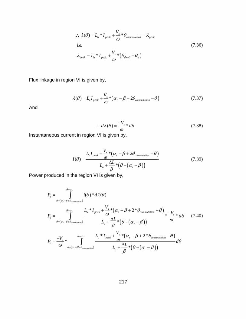
217

( ) * *

. .

* *

su peak commutation peak

speak u peak dwell a

VL I

i e

VL I

(7.36)

Flux linkage in region VI is given by,

( ) * 2su peak r commutation

VL I

(7.37)

And

( ) *sVd d

(7.38)

Instantaneous current in region VI is given by,

* 2

( )

*

su peak r commutation

u r

VL I

IL

L

(7.39)

Power produced in the region VI is given by,

6

6

6

( )* ( )

* * 2*

* *

*

* * 2*

*

*

r

r commutation

r

r commutation

r

r commutation

su peak r commutation

s

u r

su peak r commutation

s

u r

P i d

VL I

VP d

LL

VL I

VP d

LL

(7.40)

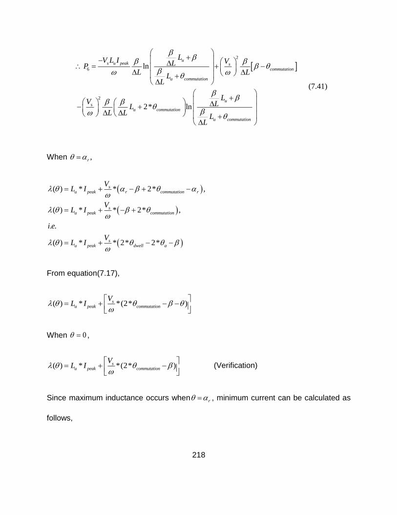
218

2

6

2

ln

2* ln

us u peak s

commutation

u commutation

us

u commutation

u commutation

LV L I VLPL L

LL

LV LL

L LL

L

(7.41)

When ,r

( ) * * 2* ,

( ) * * 2* ,

. .

( ) * * 2* 2*

su peak r commutation r

su peak commutation

su peak dwell a

VL I

VL I

i e

VL I

From equation(7.17),

( ) * *(2* )su peak commutation

VL I

When 0 ,

( ) * *(2* )su peak commutation

VL I

(Verification)

Since maximum inductance occurs when r , minimum current can be calculated as

follows,

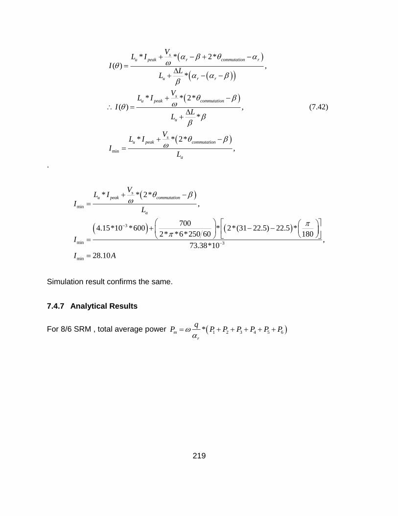
219

min

* * 2*

( ) ,

*

* * 2*

( ) ,

*

* * 2*

,

su peak r commutation r

u r r

su peak commutation

u

su peak commutation

a

VL I

IL

L

VL I

IL

L

VL I

IL

(7.42)

.

min

3

min 3

min

* * 2*

,

7004.15*10 *600 * 2*(31 22.5) 22.5 *

2* *6*250 60 180,

73.38*10

28.10

su peak commutation

a

VL I

IL

I

I A

Simulation result confirms the same.

7.4.7 Analytical Results

For 8/6 SRM , total average power 1 2 3 4 5 6*m

r

qP P P P P P P

220

2

2

*

( )ln ( )

( )2* ln

ln

( )

m

r

a r as u peak s

r a

a

a r as

commutation a

a

as u peak

a r a

qP

LV L I VL

L LL

L

LV LL

L LL

L

LV L I L

LL

L

2

2

2

22 2

2

2* 2* ln

( )

2 22* 2*

12* 2*

2

sa r

as

a r dwell

r a a

s peak r dwell sr dwell r dwell

u

sr dwell

u

V

L

LV LL

L LL

L

V I V

L

V

L

2 2

2

ln ln

ln

u ucommutation commutation

s u peak s scommutation u

u u

us u peak s

commuta

u commutation

L LV L I V VL LL

L LL L L

L L

LV L I VL

L LL

L

2

2* ln

tion

us

u commutation

u commutation

LV LL

L LL

L

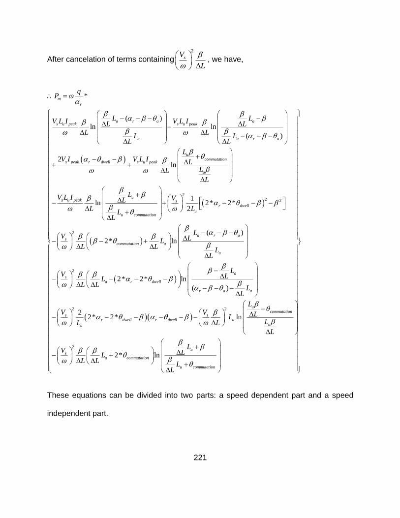
221

After cancelation of terms containing

2

sV

L

, we have,

*

( )ln ln

( )

2ln

ln

m

r

a r a as u peak s u peak

a a r a

ucommutation

s peak r dwell s u peak

u

us u peak

u

qP

L LV L I V L IL L

L LL L

L L

LV I V L I L

LL

L

LV L I L

LL

L

22 2

2

2

12* 2*

2

( )2* ln

2* 2* ln

( )

sr dwell

ucommutation

a r as

commutation a

a

as

a r dwell

r a a

V

L

LV LL

L LL

L

LV LL

L LL

L

2 2

2

22* 2* ln

2* ln

ucommutation

s sr dwell r dwell u

uu

us

u commutation

u commutation

LV V LL

LL L

L

LV LL

L LL

L

These equations can be divided into two parts: a speed dependent part and a speed

independent part.

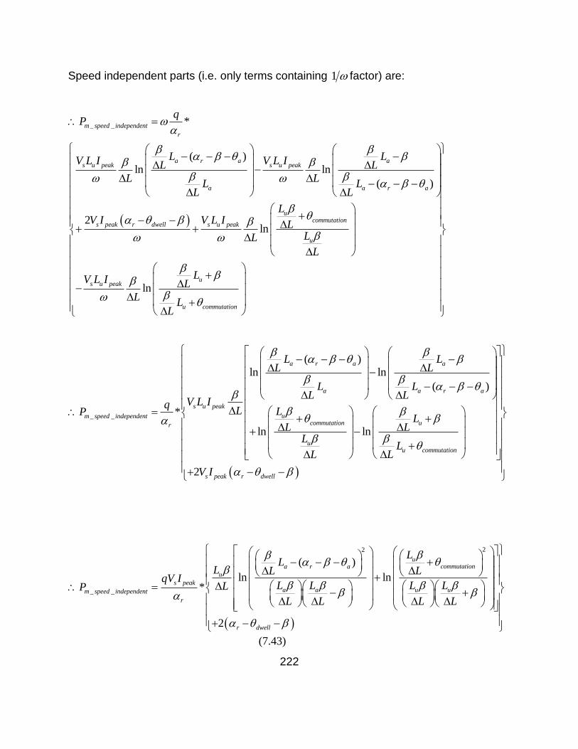
222

Speed independent parts (i.e. only terms containing 1 factor) are:

_ _ *

( )ln ln

( )

2ln

m speed independent

r

a r a as u peak s u peak

a a r a

ucommutation

s peak r dwell s u peak

u

s u peak

qP

L LV L I V L IL L

L LL L

L L

LV I V L I L

LL

L

V L I

lnu

u commutation

LL

LL

L

_ _

( )ln ln

( )

*

ln ln

a r a a

a a r a

s u peak

um speed independentcommutation ur

uu commutation

L LL L

L LL L

V L IqL LP

LL L

LL

LL

2 s peak r dwellV I

22

_ _

( )

ln ln*

2

ucommutationa r a

u

s peaka a u um speed independent

r

r dwell

LL

L LLqV I

L L L LLP

L L L L

(7.43)

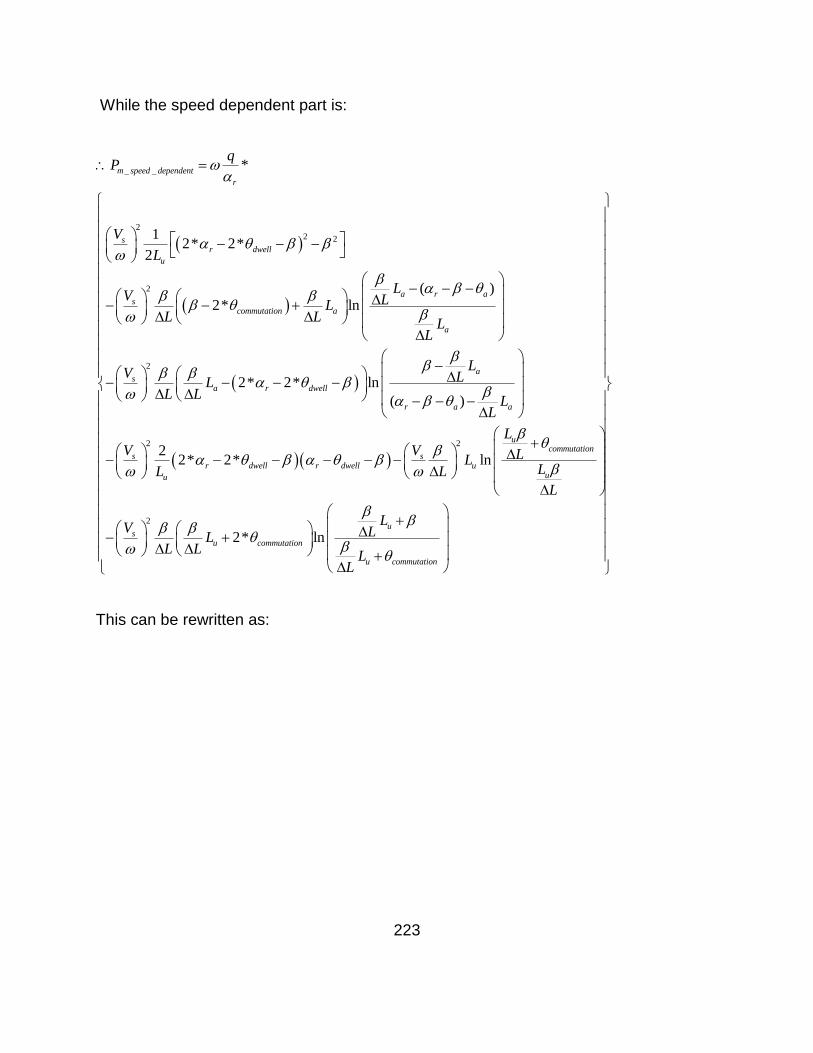
223

While the speed dependent part is:

_ _

22 2

2

2

*

12* 2*

2

( )2* ln

2* 2* ln

( )

m speed dependent

r

sr dwell

u

a r as

commutation a

a

as

a r dwell

r a

qP

V

L

LV LL

L LL

L

LV LL

L LL

L

2 2

2

22* 2* ln

2* ln

a

ucommutation

s sr dwell r dwell u

uu

us

u commutation

u commutation

LV V LL

LL L

L

LV LL

L LL

L

This can be rewritten as:

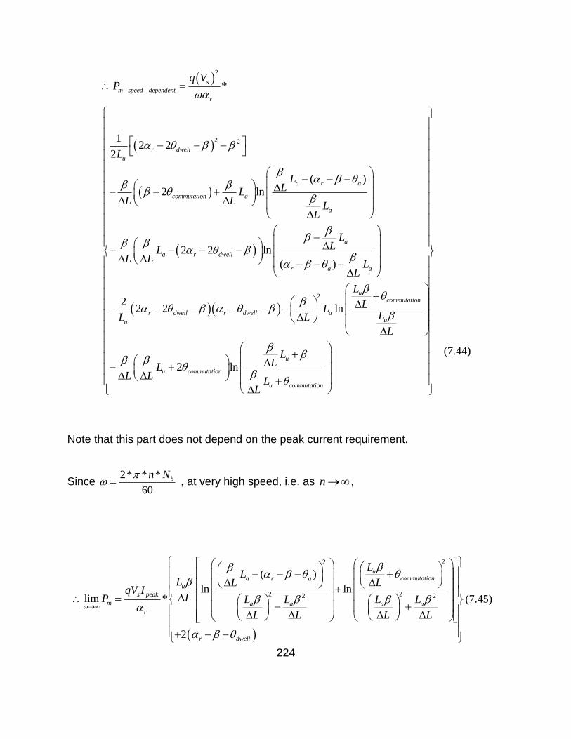
224

2

_ _

2 2

*

12 2

2

( )2 ln

2 2 ln

( )

22 2

s

m speed dependent

r

r dwell

u

a r a

commutation a

a

a

a r dwell

r a a

r dwell r

u

q VP

L

LLL

L LL

L

LLL

L LL

L

L

2

ln

2 ln

ucommutation

dwell uu

u

u commutation

u commutation

L

LLLL

L

LLL

L LL

L

(7.44)

Note that this part does not depend on the peak current requirement.

Since 2* * *

60

bn N , at very high speed, i.e. as n ,

22

2 22 2

( )

ln lnlim *

2

ucommutationa r a

u

s peak

m a a u u

r

r dwell

LL

L LLqV I

LP L L L L

L L L L

(7.45)

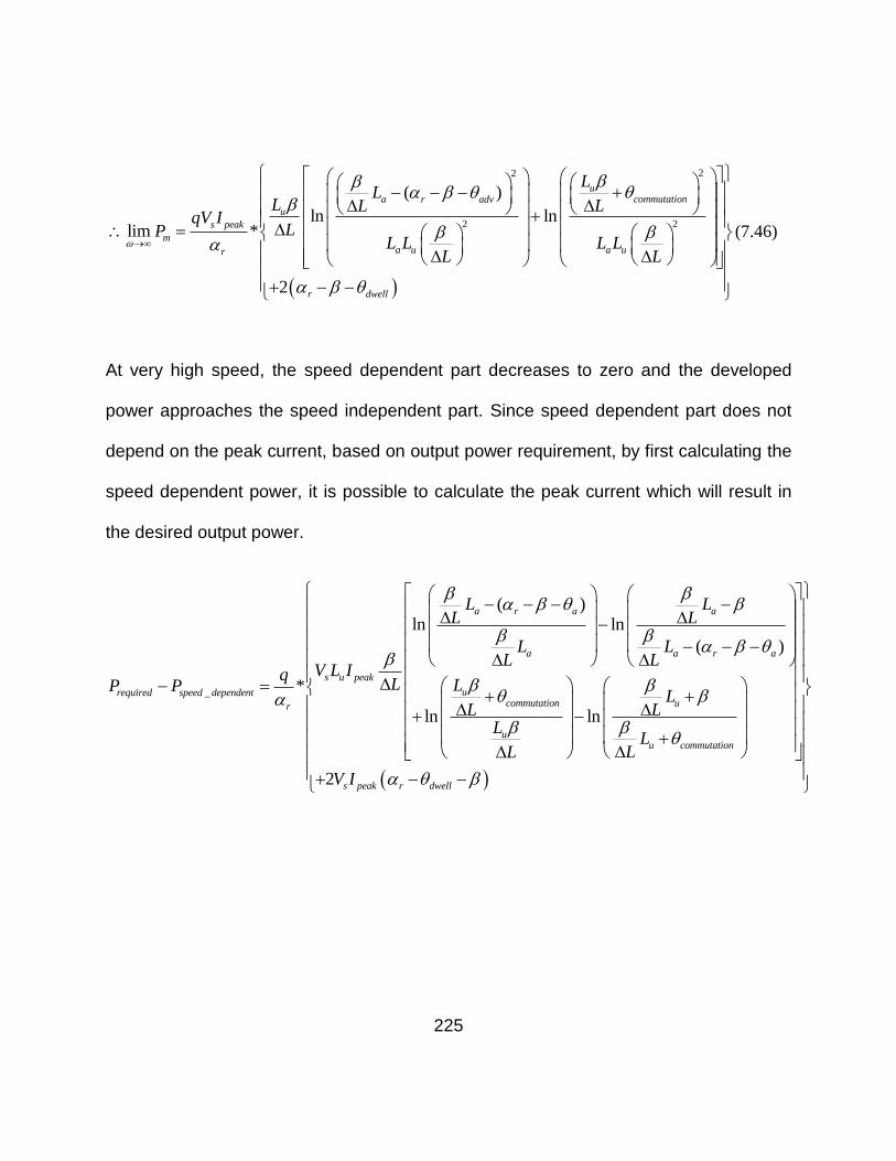
225

22

2 2

( )

ln lnlim *

2

ucommutationa r adv

u

s peak

m

a u a ur

r dwell

LL

L LLqV I

LPL L L L

L L

(7.46)

At very high speed, the speed dependent part decreases to zero and the developed

power approaches the speed independent part. Since speed dependent part does not

depend on the peak current, based on output power requirement, by first calculating the

speed dependent power, it is possible to calculate the peak current which will result in

the desired output power.

_

( )ln ln

( )

*

ln ln

a r a a

a a r a

s u peak

urequired speed dependentcommutation ur

uu commutation

L LL L

L LL L

V L IqL LP P

LL L

LL

LL

2 s peak r dwellV I

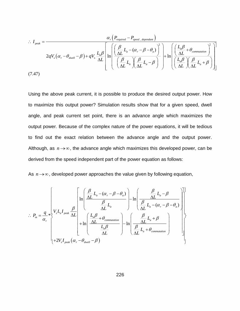
226

_

22

( )

2 ln ln

r required speed dependant

peak

ucommutationa r a

us r dwell s

ua a u

P PI

LL

L LLqV qV

LLL L L

L L L L

(7.47)

Using the above peak current, it is possible to produce the desired output power. How

to maximize this output power? Simulation results show that for a given speed, dwell

angle, and peak current set point, there is an advance angle which maximizes the

output power. Because of the complex nature of the power equations, it will be tedious

to find out the exact relation between the advance angle and the output power.

Although, as n , the advance angle which maximizes this developed power, can be

derived from the speed independent part of the power equation as follows:

As n , developed power approaches the value given by following equation,

( )ln ln

( )

*

ln ln

2

a r a a

a a r a

s u peak

umcommutation ur

uu commutation

s peak r dwel

L LL L

L LL L

V L IqL LP

LL L

LL

LL

V I

l

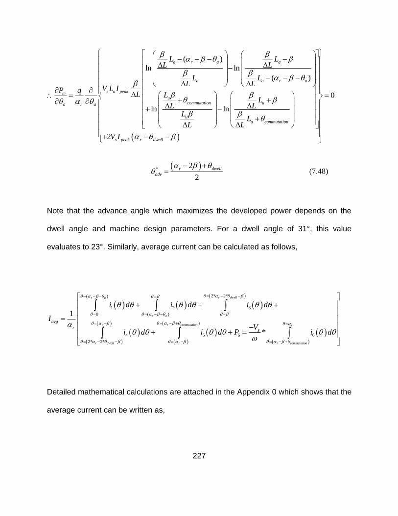
227

( )ln ln

( )

ln ln

2

a r a a

a a r a

s u peakmu

commutation ua r a

uu commutation

s peak

L LL L

L LL L

V L IP qL L

LL L

LL

LL

V I

0

r dwell

*

2

2

r dwell

adv

(7.48)

Note that the advance angle which maximizes the developed power depends on the

dwell angle and machine design parameters. For a dwell angle of 31°, this value

evaluates to 23°. Similarly, average current can be calculated as follows,

2* 2*( )

1 2 3

0 ( )

4 5 6 6

2* 2*

1

*

r dwellr a

r a

r commutationr r

r dwell r r commutation

avg

rs

i d i d i d

IV

i d i d P i d

Detailed mathematical calculations are attached in the Appendix 0 which shows that the

average current can be written as,

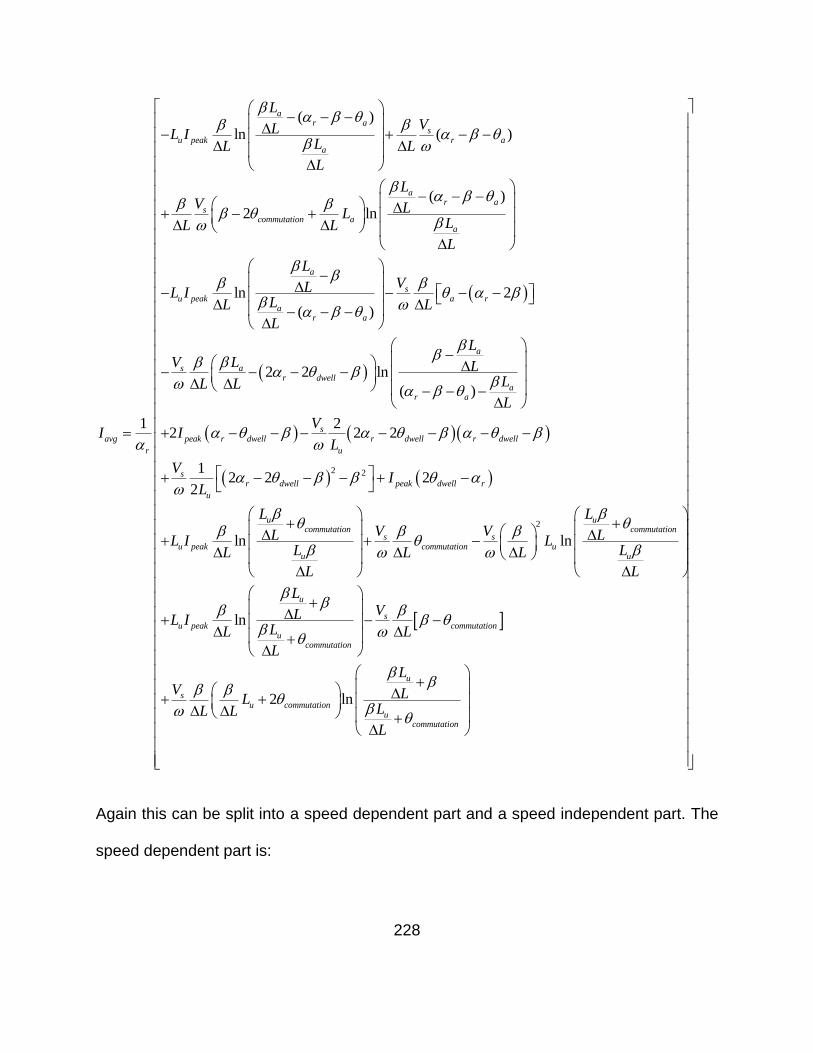
228

( )ln ( )

( )2 ln

ln 2

( )

1

ar a

su peak r a

a

ar a

scommutation a

a

a

su peak a r

ar a

s

avg

r

LVLL I

LL L

L

LV LL

LL L

L

LVLL I

LL L

L

V

I

2 2

2 2 ln

( )

22 2 2

12 2 2

2

ln

a

ar dwell

ar a

speak r dwell r dwell r dwell

u

sr dwell peak dwell r

u

ucommutation

u peaku

LL L

LL L

L

VI

L

VI

L

L

LL ILL

L

2

ln

ln

2 ln

ucommutation

s scommutation u

u

u

su peak commutation

ucommutation

u

su commutation

ucommutatio

LV V LL

LL L

L

LVLL I

LL L

L

LV LL

LL L

L

n

Again this can be split into a speed dependent part and a speed independent part. The

speed dependent part is:

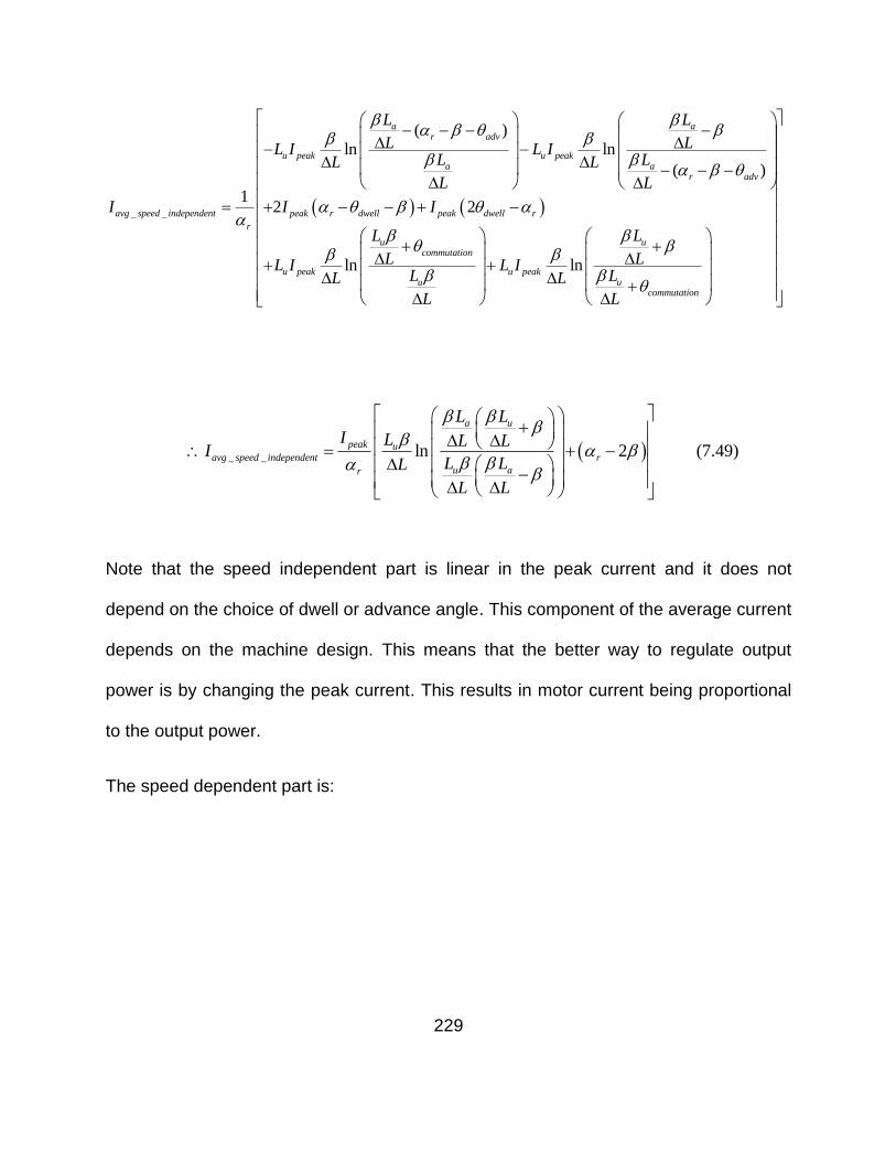
229

_ _

( )ln ln

( )

12 2

ln

a ar adv

u peak u peaka a

r adv

avg speed independent peak r dwell peak dwell r

r

ucommutation

u peaku

L L

L LL I L IL LL L

L L

I I I

L

LL I LLL

L

ln

u

u peaku

commutation

L

LILL

L

_ _ ln 2

a u

peak uavg speed independent r

u ar

L L

I L L LI

L LL

L L

(7.49)

Note that the speed independent part is linear in the peak current and it does not

depend on the choice of dwell or advance angle. This component of the average current

depends on the machine design. This means that the better way to regulate output

power is by changing the peak current. This results in motor current being proportional

to the output power.

The speed dependent part is:

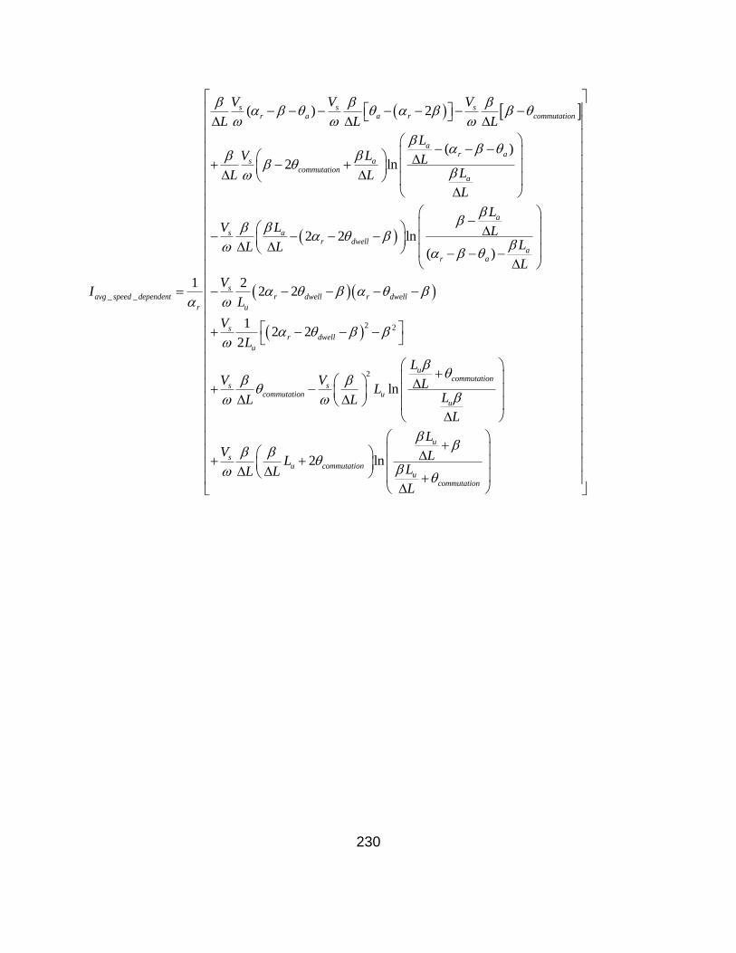
230

_ _

( ) 2

( )2 ln

2 2 ln

( )

1

s s sr a a r commutation

ar a

s acommutation

a

a

s ar dwell

ar a

avg speed dependent

r

V V V

L L L

LV L L

LL L

L

LV L L

LL L

I

2 2

2

22 2

12 2

2

ln

2 ln

sr dwell r dwell

u

sr dwell

u

ucommutation

s scommutation u

u

u

su commutation

ucommutation

L

V

L

V

L

LV V LL

LL L

L

LV LL

LL L

L

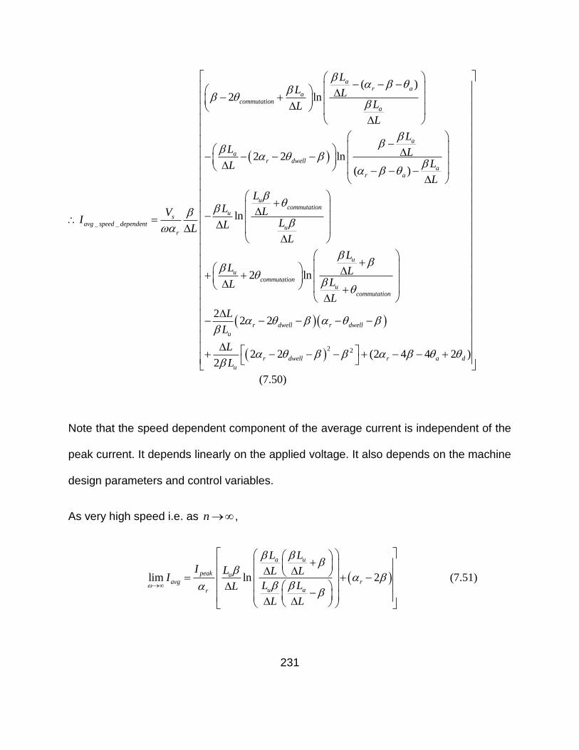
231

_ _

( )2 ln

2 2 ln

( )

ln

2

ar a

acommutation

a

a

ar dwell

ar a

ucommutation

us

avg speed dependentu

r

uc

LL L

LL

L

LL L

LL

L

LL LV

I LLLL

L

L

2 2

ln

22 2

2 2 (2 4 4 2 )2

u

ommutationu

commutation

r dwell r dwell

u

r dwell r a d

u

L

LL

L

L

L

L

L

(7.50)

Note that the speed dependent component of the average current is independent of the

peak current. It depends linearly on the applied voltage. It also depends on the machine

design parameters and control variables.

As very high speed i.e. as n ,

lim ln 2

a u

peak uavg r

u ar

L L

I L L LI

L LL

L L

(7.51)

232

This equation can be simplified to the following form,

lim 2 ln 2peak u a

avg r

r u

I L LI

L L

(7.52)

Note that, for a fixed machine design, at high speed, the average current only depends

on the peak current and does not depend on the advance angle or the dwell angle.

At high speed, the developed power is,

22

2 2

( )

ln lnlim *

2

ucommutationa r a

u

s peak

m

a u a ur

r dwell

LL

L LLqV I

LPL L L L

L L

This power can be maximized using, *

2

r dwell

adv

For 2

rdwell

, * 3

4adv r . This formula agrees with the result of linear analysis

described in [13] and [78]. Number of strokes required to achieve steady state can be

derived. Initially, during each cycle, since the dwell angle is more than half of the rotor

pole pitch, fluxing region is going to be more than de-fluxing region. Therefore at the

end of each stroke, initial flux linkage will increase by,

* 2* ,sadd dwell r

V

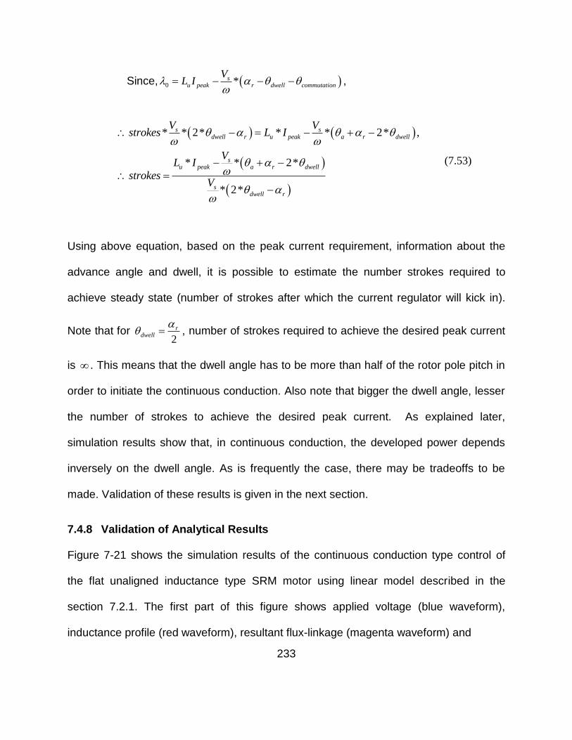
233

Since, 0 *su peak r dwell commutation

VL I

,

* * 2* * * 2* ,

* * 2*

* 2*

s sdwell r u peak a r dwell

su peak a r dwell

sdwell r

V Vstrokes L I

VL I

strokesV

(7.53)

Using above equation, based on the peak current requirement, information about the

advance angle and dwell, it is possible to estimate the number strokes required to

achieve steady state (number of strokes after which the current regulator will kick in).

Note that for 2

rdwell

, number of strokes required to achieve the desired peak current

is . This means that the dwell angle has to be more than half of the rotor pole pitch in

order to initiate the continuous conduction. Also note that bigger the dwell angle, lesser

the number of strokes to achieve the desired peak current. As explained later,

simulation results show that, in continuous conduction, the developed power depends

inversely on the dwell angle. As is frequently the case, there may be tradeoffs to be

made. Validation of these results is given in the next section.

7.4.8 Validation of Analytical Results

Figure 7-21 shows the simulation results of the continuous conduction type control of

the flat unaligned inductance type SRM motor using linear model described in the

section 7.2.1. The first part of this figure shows applied voltage (blue waveform),

inductance profile (red waveform), resultant flux-linkage (magenta waveform) and

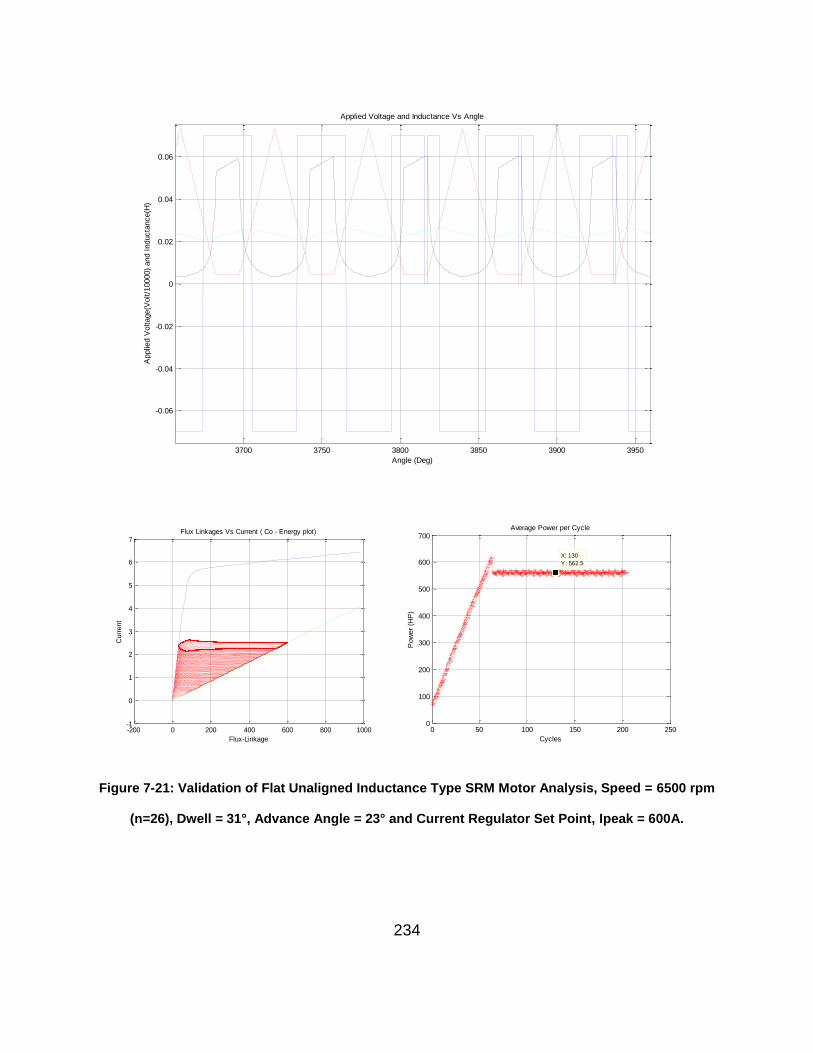
234

Figure 7-21: Validation of Flat Unaligned Inductance Type SRM Motor Analysis, Speed = 6500 rpm

(n=26), Dwell = 31°, Advance Angle = 23° and Current Regulator Set Point, Ipeak = 600A.

3700 3750 3800 3850 3900 3950

-0.06

-0.04

-0.02

0

0.02

0.04

0.06

Angle (Deg)

Applie

d V

oltage(V

olt/1

0000)

and I

nducta

nce(H

)

Applied Voltage and Inductance Vs Angle

-200 0 200 400 600 800 1000-1

0

1

2

3

4

5

6

7

Flux-Linkage

Curr

ent

Flux Linkages Vs Current ( Co - Energy plot)

0 50 100 150 200 2500

100

200

300

400

500

600

700

X: 130

Y: 562.5

Cycles

Pow

er

(HP

)

Average Power per Cycle

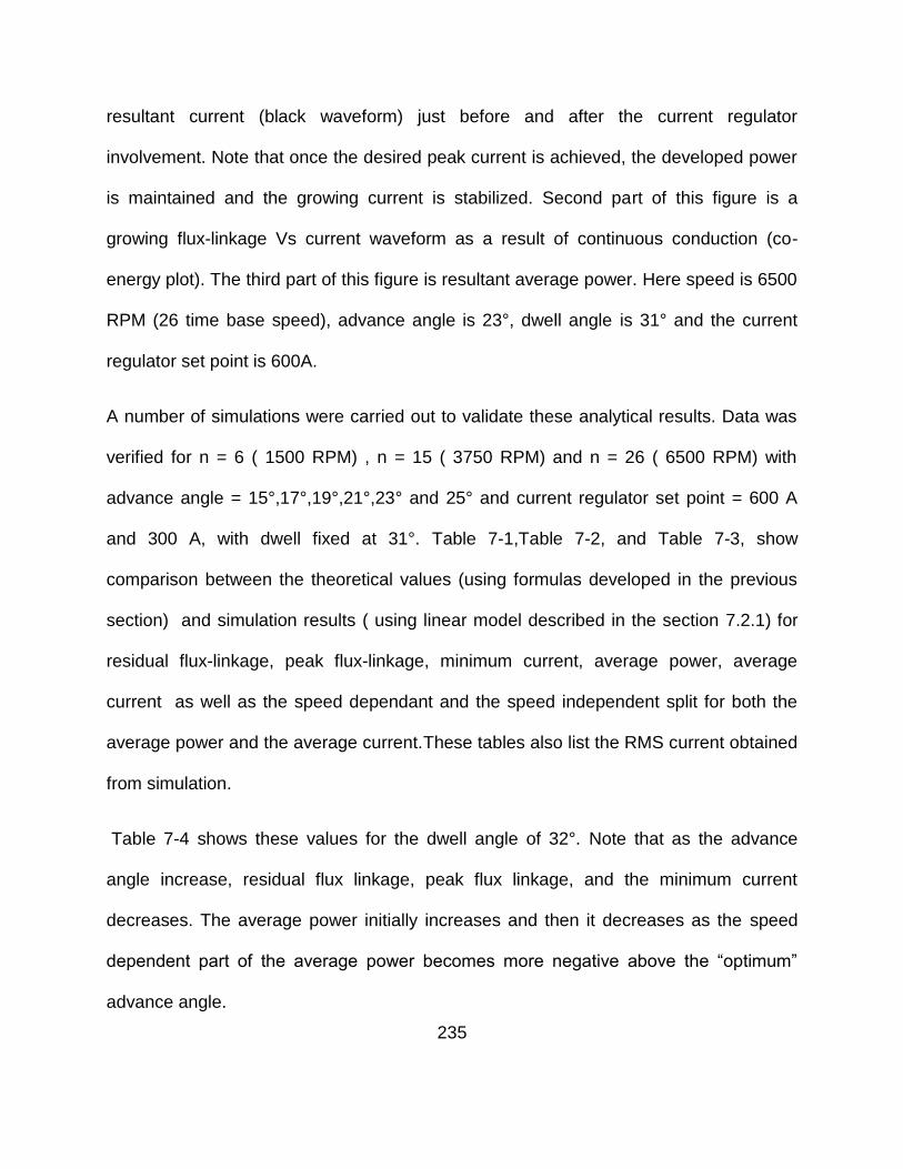
235

resultant current (black waveform) just before and after the current regulator

involvement. Note that once the desired peak current is achieved, the developed power

is maintained and the growing current is stabilized. Second part of this figure is a

growing flux-linkage Vs current waveform as a result of continuous conduction (co-

energy plot). The third part of this figure is resultant average power. Here speed is 6500

RPM (26 time base speed), advance angle is 23°, dwell angle is 31° and the current

regulator set point is 600A.

A number of simulations were carried out to validate these analytical results. Data was

verified for n = 6 ( 1500 RPM) , n = 15 ( 3750 RPM) and n = 26 ( 6500 RPM) with

advance angle = 15°,17°,19°,21°,23° and 25° and current regulator set point = 600 A

and 300 A, with dwell fixed at 31°. Table 7-1,Table 7-2, and Table 7-3, show

comparison between the theoretical values (using formulas developed in the previous

section) and simulation results ( using linear model described in the section 7.2.1) for

residual flux-linkage, peak flux-linkage, minimum current, average power, average

current as well as the speed dependant and the speed independent split for both the

average power and the average current.These tables also list the RMS current obtained

from simulation.

Table 7-4 shows these values for the dwell angle of 32°. Note that as the advance

angle increase, residual flux linkage, peak flux linkage, and the minimum current

decreases. The average power initially increases and then it decreases as the speed

dependent part of the average power becomes more negative above the “optimum”

advance angle.

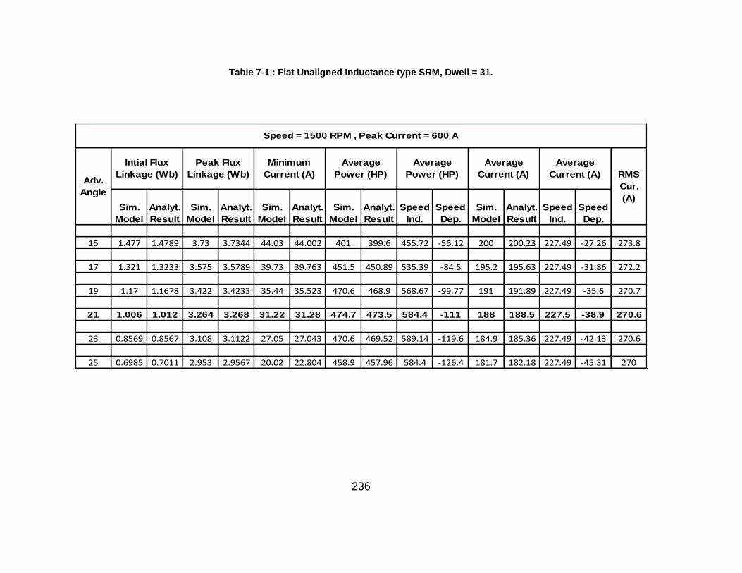
236

Table 7-1 : Flat Unaligned Inductance type SRM, Dwell = 31.

Sim.

Model

Analyt.

Result

Sim.

Model

Analyt.

Result

Sim.

Model

Analyt.

Result

Sim.

Model

Analyt.

Result

Speed

Ind.

Speed

Dep.

Sim.

Model

Analyt.

Result

Speed

Ind.

Speed

Dep.

15 1.477 1.4789 3.73 3.7344 44.03 44.002 401 399.6 455.72 -56.12 200 200.23 227.49 -27.26 273.8

17 1.321 1.3233 3.575 3.5789 39.73 39.763 451.5 450.89 535.39 -84.5 195.2 195.63 227.49 -31.86 272.2

19 1.17 1.1678 3.422 3.4233 35.44 35.523 470.6 468.9 568.67 -99.77 191 191.89 227.49 -35.6 270.7

21 1.006 1.012 3.264 3.268 31.22 31.28 474.7 473.5 584.4 -111 188 188.5 227.5 -38.9 270.6

23 0.8569 0.8567 3.108 3.1122 27.05 27.043 470.6 469.52 589.14 -119.6 184.9 185.36 227.49 -42.13 270.6

25 0.6985 0.7011 2.953 2.9567 20.02 22.804 458.9 457.96 584.4 -126.4 181.7 182.18 227.49 -45.31 270

RMS

Cur.

(A)

Speed = 1500 RPM , Peak Current = 600 A

Adv.

Angle

Intial Flux

Linkage (Wb)

Peak Flux

Linkage (Wb)

Minimum

Current (A)

Average

Power (HP)

Average

Power (HP)

Average

Current (A)

Average

Current (A)

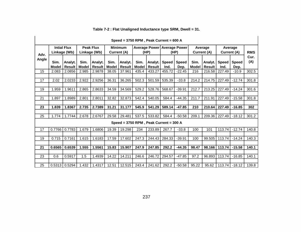
237

Table 7-2 : Flat Unaligned Inductance type SRM, Dwell = 31.

Sim.

Model

Analyt.

Result

Sim.

Model

Analyt.

Result

Sim.

Model

Analyt.

Result

Sim.

Model

Analyt.

Result

Speed

Ind.

Speed

Dep.

Sim.

Model

Analyt.

Result

Speed

Ind.

Speed

Dep.

15 2.083 2.0856 2.985 2.9878 38.05 37.961 435.4 433.27 455.72 -22.45 216 216.58 227.49 -10.9 302.5

17 2.02 2.0233 2.922 2.9256 36.31 36.265 502.3 501.59 535.39 -33.8 214.2 214.75 227.49 -12.74 301.8

19 1.959 1.9611 2.865 2.8633 34.59 34.569 529.2 528.76 568.67 -39.91 212.7 213.25 227.49 -14.24 301.6

21 1.897 1.8989 2.801 2.8011 32.82 32.873 542.4 540.05 584.4 -44.35 211.7 211.91 227.49 -15.58 301.8

23 1.839 1.8367 2.735 2.7389 31.21 31.177 545.9 541.29 589.14 -47.85 210 210.64 227.49 -16.85 302

25 1.774 1.7744 2.678 2.6767 29.58 29.481 537.5 533.82 584.4 -50.58 209.1 209.36 227.49 -18.12 301.2

17 0.7766 0.7783 1.679 1.6806 19.39 19.298 234 233.89 267.7 -33.8 100 101 113.74 -12.74 140.8

19 0.715 0.7161 1.615 1.6183 17.59 17.602 247.3 244.43 284.33 -39.91 100 99.505 113.74 -14.24 140.3

21 0.6565 0.6539 1.555 1.5561 15.83 15.907 247.9 247.85 292.2 -44.35 98.47 98.166 113.74 -15.58 140.1

23 0.6 0.5917 1.5 1.4939 14.22 14.211 246.6 246.72 294.57 -47.85 97.2 96.893 113.74 -16.85 140.1

25 0.5313 0.5294 1.432 1.4317 12.51 12.515 243.4 241.62 292.2 -50.58 95.22 95.62 113.74 -18.12 139.8

Average Power

(HP)

Average

Current (A)

Average Power

(HP) RMS

Cur.

(A)

Average

Current (A)

Speed = 3750 RPM , Peak Current = 600 A

Speed = 3750 RPM , Peak Current = 300 A

Intial Flux

Linkage (Wb)Adv.

Angle

Peak Flux

Linkage (Wb)

Minimum

Current (A)

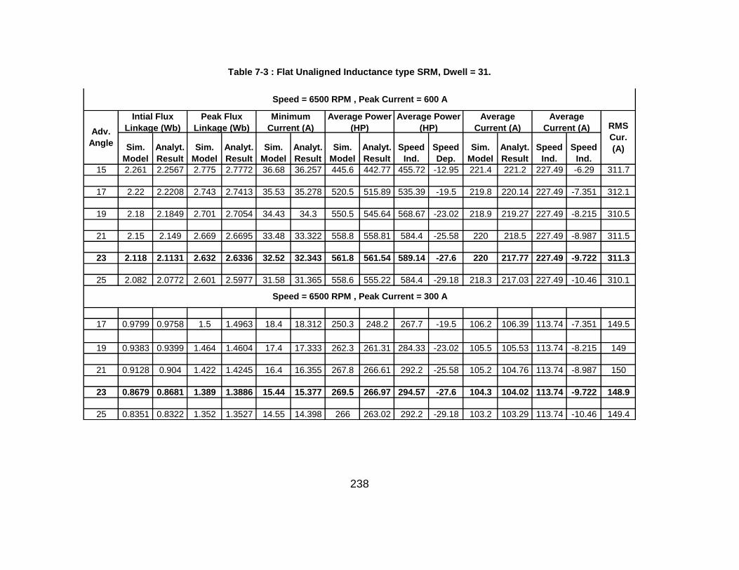
238

Table 7-3 : Flat Unaligned Inductance type SRM, Dwell = 31.

Sim.

Model

Analyt.

Result

Sim.

Model

Analyt.

Result

Sim.

Model

Analyt.

Result

Sim.

Model

Analyt.

Result

Speed

Ind.

Speed

Dep.

Sim.

Model

Analyt.

Result

Speed

Ind.

Speed

Ind.

15 2.261 2.2567 2.775 2.7772 36.68 36.257 445.6 442.77 455.72 -12.95 221.4 221.2 227.49 -6.29 311.7

17 2.22 2.2208 2.743 2.7413 35.53 35.278 520.5 515.89 535.39 -19.5 219.8 220.14 227.49 -7.351 312.1

19 2.18 2.1849 2.701 2.7054 34.43 34.3 550.5 545.64 568.67 -23.02 218.9 219.27 227.49 -8.215 310.5

21 2.15 2.149 2.669 2.6695 33.48 33.322 558.8 558.81 584.4 -25.58 220 218.5 227.49 -8.987 311.5

23 2.118 2.1131 2.632 2.6336 32.52 32.343 561.8 561.54 589.14 -27.6 220 217.77 227.49 -9.722 311.3

25 2.082 2.0772 2.601 2.5977 31.58 31.365 558.6 555.22 584.4 -29.18 218.3 217.03 227.49 -10.46 310.1

17 0.9799 0.9758 1.5 1.4963 18.4 18.312 250.3 248.2 267.7 -19.5 106.2 106.39 113.74 -7.351 149.5

19 0.9383 0.9399 1.464 1.4604 17.4 17.333 262.3 261.31 284.33 -23.02 105.5 105.53 113.74 -8.215 149

21 0.9128 0.904 1.422 1.4245 16.4 16.355 267.8 266.61 292.2 -25.58 105.2 104.76 113.74 -8.987 150

23 0.8679 0.8681 1.389 1.3886 15.44 15.377 269.5 266.97 294.57 -27.6 104.3 104.02 113.74 -9.722 148.9

25 0.8351 0.8322 1.352 1.3527 14.55 14.398 266 263.02 292.2 -29.18 103.2 103.29 113.74 -10.46 149.4

Average

Current (A) RMS

Cur.

(A)

Average Power

(HP)

Average

Current (A)

Speed = 6500 RPM , Peak Current = 600 A

Speed = 6500 RPM , Peak Current = 300 A

Intial Flux

Linkage (Wb)Adv.

Angle

Peak Flux

Linkage (Wb)

Minimum

Current (A)

Average Power

(HP)

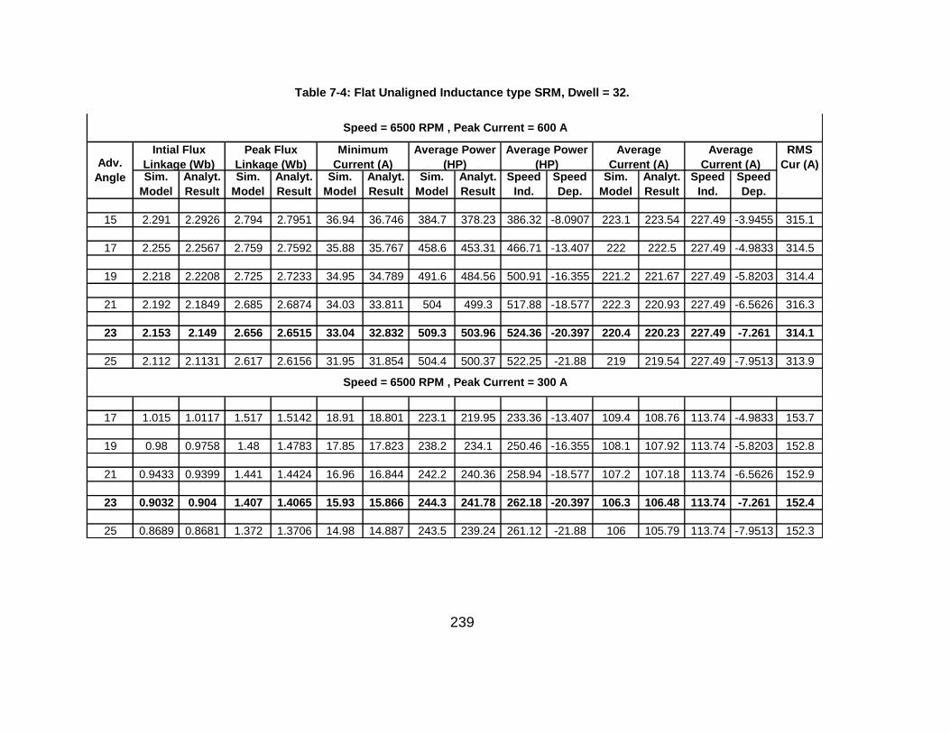
239

Table 7-4: Flat Unaligned Inductance type SRM, Dwell = 32.

Sim.

Model

Analyt.

Result

Sim.

Model

Analyt.

Result

Sim.

Model

Analyt.

Result

Sim.

Model

Analyt.

Result

Speed

Ind.

Speed

Dep.

Sim.

Model

Analyt.

Result

Speed

Ind.

Speed

Dep.

15 2.291 2.2926 2.794 2.7951 36.94 36.746 384.7 378.23 386.32 -8.0907 223.1 223.54 227.49 -3.9455 315.1

17 2.255 2.2567 2.759 2.7592 35.88 35.767 458.6 453.31 466.71 -13.407 222 222.5 227.49 -4.9833 314.5

19 2.218 2.2208 2.725 2.7233 34.95 34.789 491.6 484.56 500.91 -16.355 221.2 221.67 227.49 -5.8203 314.4

21 2.192 2.1849 2.685 2.6874 34.03 33.811 504 499.3 517.88 -18.577 222.3 220.93 227.49 -6.5626 316.3

23 2.153 2.149 2.656 2.6515 33.04 32.832 509.3 503.96 524.36 -20.397 220.4 220.23 227.49 -7.261 314.1

25 2.112 2.1131 2.617 2.6156 31.95 31.854 504.4 500.37 522.25 -21.88 219 219.54 227.49 -7.9513 313.9

17 1.015 1.0117 1.517 1.5142 18.91 18.801 223.1 219.95 233.36 -13.407 109.4 108.76 113.74 -4.9833 153.7

19 0.98 0.9758 1.48 1.4783 17.85 17.823 238.2 234.1 250.46 -16.355 108.1 107.92 113.74 -5.8203 152.8

21 0.9433 0.9399 1.441 1.4424 16.96 16.844 242.2 240.36 258.94 -18.577 107.2 107.18 113.74 -6.5626 152.9

23 0.9032 0.904 1.407 1.4065 15.93 15.866 244.3 241.78 262.18 -20.397 106.3 106.48 113.74 -7.261 152.4

25 0.8689 0.8681 1.372 1.3706 14.98 14.887 243.5 239.24 261.12 -21.88 106 105.79 113.74 -7.9513 152.3

Average Power

(HP)

RMS

Cur (A)

Average

Current (A)

Average Power

(HP)

Average

Current (A)

Speed = 6500 RPM , Peak Current = 600 A

Speed = 6500 RPM , Peak Current = 300 A

Intial Flux

Linkage (Wb)Adv.

Angle

Peak Flux

Linkage (Wb)

Minimum

Current (A)

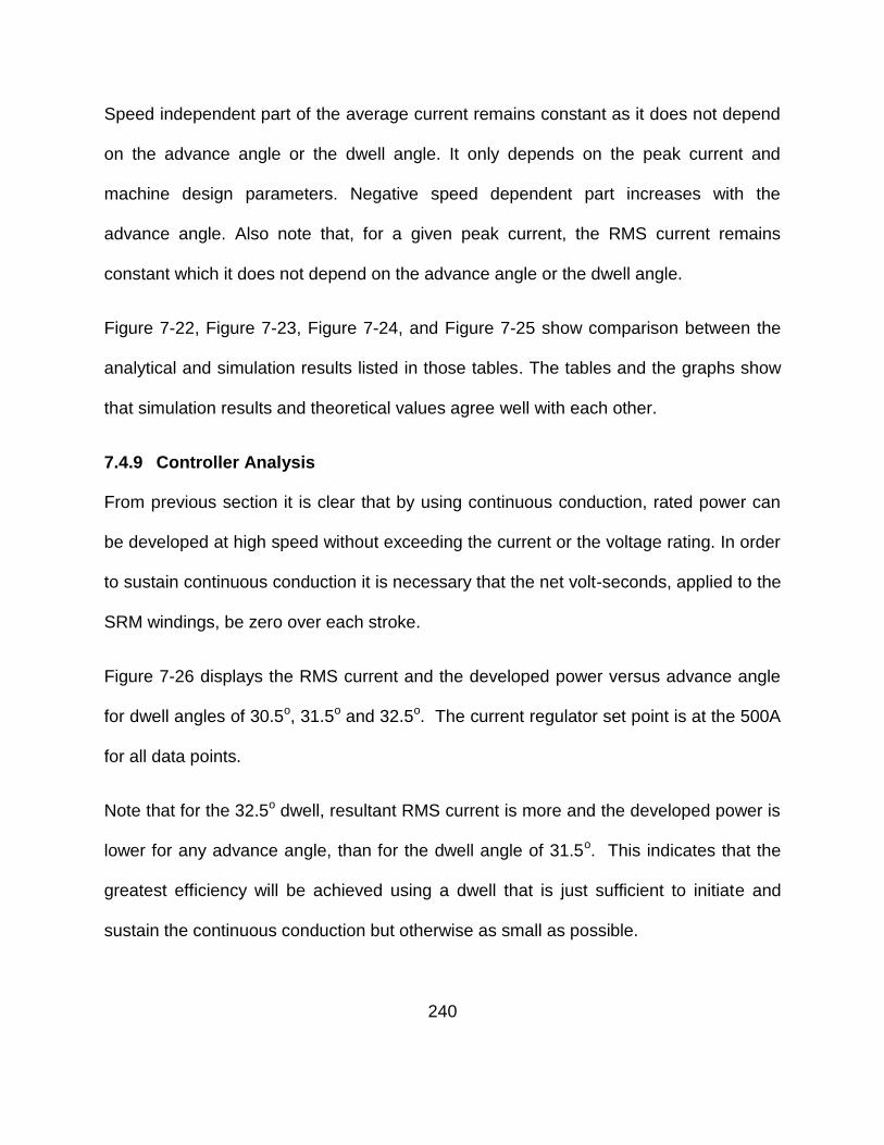
240

Speed independent part of the average current remains constant as it does not depend

on the advance angle or the dwell angle. It only depends on the peak current and

machine design parameters. Negative speed dependent part increases with the

advance angle. Also note that, for a given peak current, the RMS current remains

constant which it does not depend on the advance angle or the dwell angle.

Figure 7-22, Figure 7-23, Figure 7-24, and Figure 7-25 show comparison between the

analytical and simulation results listed in those tables. The tables and the graphs show

that simulation results and theoretical values agree well with each other.

7.4.9 Controller Analysis

From previous section it is clear that by using continuous conduction, rated power can

be developed at high speed without exceeding the current or the voltage rating. In order

to sustain continuous conduction it is necessary that the net volt-seconds, applied to the

SRM windings, be zero over each stroke.

Figure 7-26 displays the RMS current and the developed power versus advance angle

for dwell angles of 30.5o, 31.5o and 32.5o. The current regulator set point is at the 500A

for all data points.

Note that for the 32.5o dwell, resultant RMS current is more and the developed power is

lower for any advance angle, than for the dwell angle of 31.5o. This indicates that the

greatest efficiency will be achieved using a dwell that is just sufficient to initiate and

sustain the continuous conduction but otherwise as small as possible.

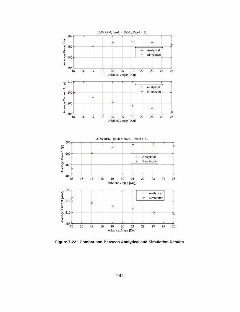
241

Figure 7-22 : Comparison Between Analytical and Simulation Results.

15 16 17 18 19 20 21 22 23 24 25350

400

450

500

Advance Angle [Deg]

Avera

ge P

ow

er

[hp]

1500 RPM, Ipeak = 600A , Dwell = 31

Analytical

Simulation

15 16 17 18 19 20 21 22 23 24 25180

190

200

210

Advance Angle [Deg]

Avera

ge C

urr

ent

[Am

p]

Analytical

Simulation

15 16 17 18 19 20 21 22 23 24 25400

450

500

550

Advance Angle [Deg]

Avera

ge P

ow

er

[hp]

3750 RPM, Ipeak = 600A , Dwell = 31

Analytical

Simulation

15 16 17 18 19 20 21 22 23 24 25205

210

215

220

Advance Angle [Deg]

Avera

ge C

urr

ent

[Am

p]

Analytical

Simulation

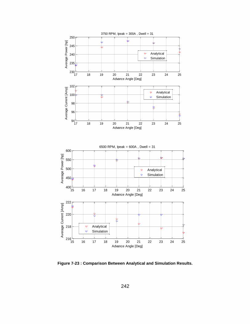
242

Figure 7-23 : Comparison Between Analytical and Simulation Results.

17 18 19 20 21 22 23 24 25230

235

240

245

250

Advance Angle [Deg]

Avera

ge P

ow

er

[hp]

3750 RPM, Ipeak = 300A , Dwell = 31

Analytical

Simulation

17 18 19 20 21 22 23 24 2594

96

98

100

102

Advance Angle [Deg]

Avera

ge C

urr

ent

[Am

p]

Analytical

Simulation

15 16 17 18 19 20 21 22 23 24 25400

450

500

550

600

Advance Angle [Deg]

Avera

ge P

ow

er

[hp]

6500 RPM, Ipeak = 600A , Dwell = 31

Analytical

Simulation

15 16 17 18 19 20 21 22 23 24 25216

218

220

222

Advance Angle [Deg]

Avera

ge C

urr

ent

[Am

p]

Analytical

Simulation

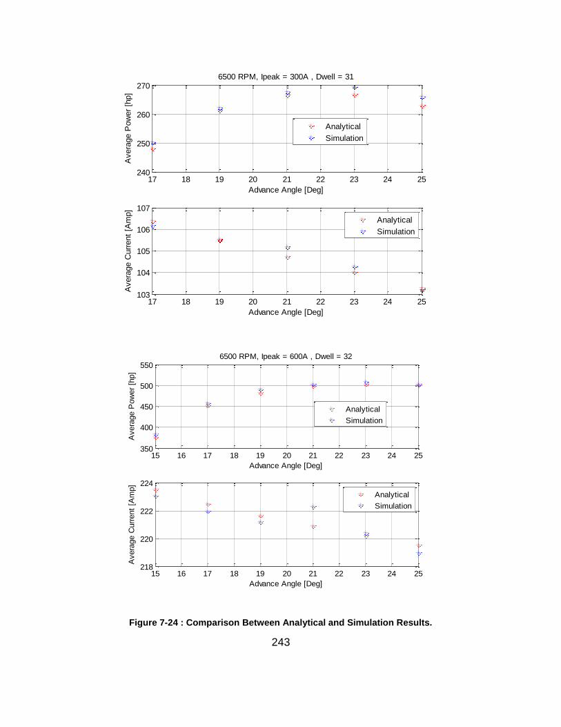
243

Figure 7-24 : Comparison Between Analytical and Simulation Results.

17 18 19 20 21 22 23 24 25240

250

260

270

Advance Angle [Deg]

Avera

ge P

ow

er

[hp]

6500 RPM, Ipeak = 300A , Dwell = 31

Analytical

Simulation

17 18 19 20 21 22 23 24 25103

104

105

106

107

Advance Angle [Deg]

Avera

ge C

urr

ent

[Am

p]

Analytical

Simulation

15 16 17 18 19 20 21 22 23 24 25350

400

450

500

550

Advance Angle [Deg]

Avera

ge P

ow

er

[hp]

6500 RPM, Ipeak = 600A , Dwell = 32

Analytical

Simulation

15 16 17 18 19 20 21 22 23 24 25218

220

222

224

Advance Angle [Deg]

Avera

ge C

urr

ent

[Am

p]

Analytical

Simulation

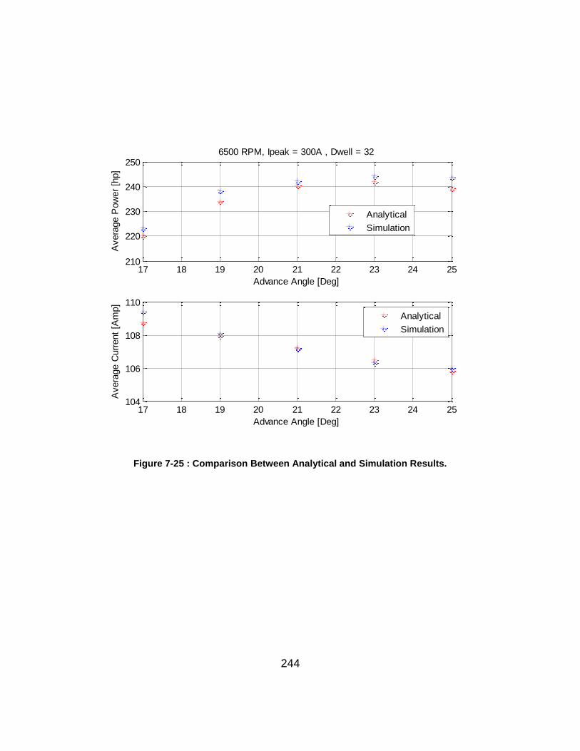
244

Figure 7-25 : Comparison Between Analytical and Simulation Results.

17 18 19 20 21 22 23 24 25210

220

230

240

250

Advance Angle [Deg]

Avera

ge P

ow

er

[hp]

6500 RPM, Ipeak = 300A , Dwell = 32

Analytical

Simulation

17 18 19 20 21 22 23 24 25104

106

108

110

Advance Angle [Deg]

Avera

ge C

urr

ent

[Am

p]

Analytical

Simulation

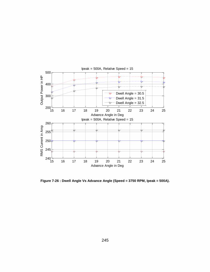
245

Figure 7-26 : Dwell Angle Vs Advance Angle (Speed = 3750 RPM, Ipeak = 500A).

15 16 17 18 19 20 21 22 23 24 25200

300

400

500

Advance Angle in Deg

Outp

ut

Pow

er

in H

P

Ipeak = 500A, Relative Speed = 15

Dwell Angle = 30.5

Dwell Angle = 31.5

Dwell Angle = 32.5

15 16 17 18 19 20 21 22 23 24 25240

245

250

255

260

Advance Angle in Deg

RM

S C

urr

ent

in A

mp

Ipeak = 500A, Relative Speed = 15

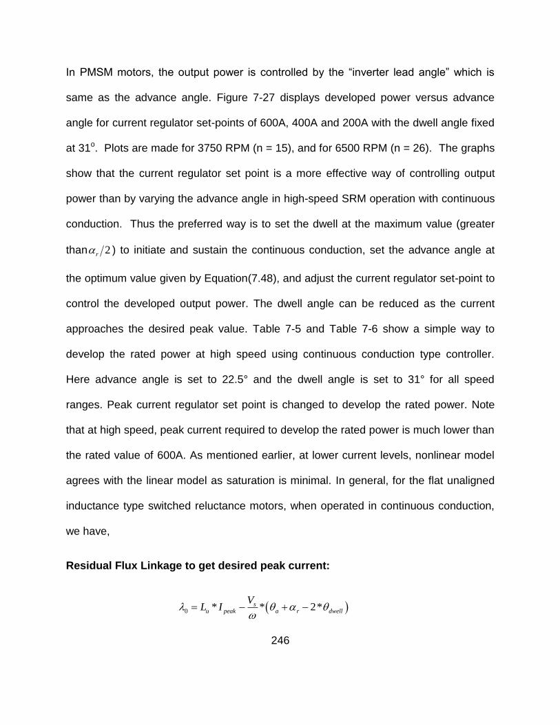
246

In PMSM motors, the output power is controlled by the “inverter lead angle” which is

same as the advance angle. Figure 7-27 displays developed power versus advance

angle for current regulator set-points of 600A, 400A and 200A with the dwell angle fixed

at 31o. Plots are made for 3750 RPM (n = 15), and for 6500 RPM (n = 26). The graphs

show that the current regulator set point is a more effective way of controlling output

power than by varying the advance angle in high-speed SRM operation with continuous

conduction. Thus the preferred way is to set the dwell at the maximum value (greater

than 2r ) to initiate and sustain the continuous conduction, set the advance angle at

the optimum value given by Equation(7.48), and adjust the current regulator set-point to

control the developed output power. The dwell angle can be reduced as the current

approaches the desired peak value. Table 7-5 and Table 7-6 show a simple way to

develop the rated power at high speed using continuous conduction type controller.

Here advance angle is set to 22.5° and the dwell angle is set to 31° for all speed

ranges. Peak current regulator set point is changed to develop the rated power. Note

that at high speed, peak current required to develop the rated power is much lower than

the rated value of 600A. As mentioned earlier, at lower current levels, nonlinear model

agrees with the linear model as saturation is minimal. In general, for the flat unaligned

inductance type switched reluctance motors, when operated in continuous conduction,

we have,

Residual Flux Linkage to get desired peak current:

0 * * 2*su peak a r dwell

VL I

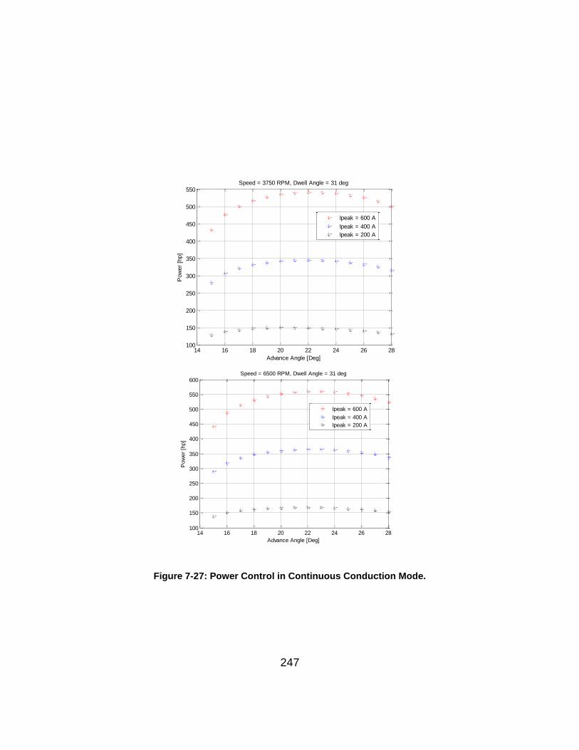
247

Figure 7-27: Power Control in Continuous Conduction Mode.

14 16 18 20 22 24 26 28100

150

200

250

300

350

400

450

500

550

Advance Angle [Deg]

Pow

er

[hp]

Speed = 3750 RPM, Dwell Angle = 31 deg

Ipeak = 600 A

Ipeak = 400 A

Ipeak = 200 A

14 16 18 20 22 24 26 28100

150

200

250

300

350

400

450

500

550

600

Advance Angle [Deg]

Pow

er

[hp]

Speed = 6500 RPM, Dwell Angle = 31 deg

Ipeak = 600 A

Ipeak = 400 A

Ipeak = 200 A

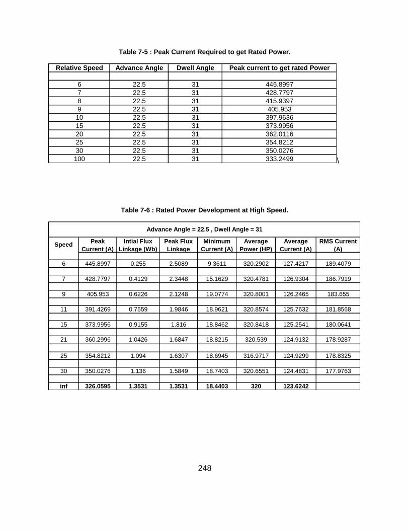
248

Table 7-5 : Peak Current Required to get Rated Power.

Relative Speed Advance Angle Dwell Angle Peak current to get rated Power

6 22.5 31 445.8997

7 22.5 31 428.7797

8 22.5 31 415.9397

9 22.5 31 405.953

10 22.5 31 397.9636

15 22.5 31 373.9956

20 22.5 31 362.0116

25 22.5 31 354.8212

30 22.5 31 350.0276

100 22.5 31 333.2499 \

Table 7-6 : Rated Power Development at High Speed.

6 445.8997 0.255 2.5089 9.3611 320.2902 127.4217 189.4079

7 428.7797 0.4129 2.3448 15.1629 320.4781 126.9304 186.7919

9 405.953 0.6226 2.1248 19.0774 320.8001 126.2465 183.655

11 391.4269 0.7559 1.9846 18.9621 320.8574 125.7632 181.8568

15 373.9956 0.9155 1.816 18.8462 320.8418 125.2541 180.0641

21 360.2996 1.0426 1.6847 18.8215 320.539 124.9132 178.9287

25 354.8212 1.094 1.6307 18.6945 316.9717 124.9299 178.8325

30 350.0276 1.136 1.5849 18.7403 320.6551 124.4831 177.9763

inf 326.0595 1.3531 1.3531 18.4403 320 123.6242

Advance Angle = 22.5 , Dwell Angle = 31

Average

Current (A)

Intial Flux

Linkage (Wb)Speed

Peak Flux

Linkage

Minimum

Current (A)

Average

Power (HP)

RMS Current

(A)

Peak

Current (A)

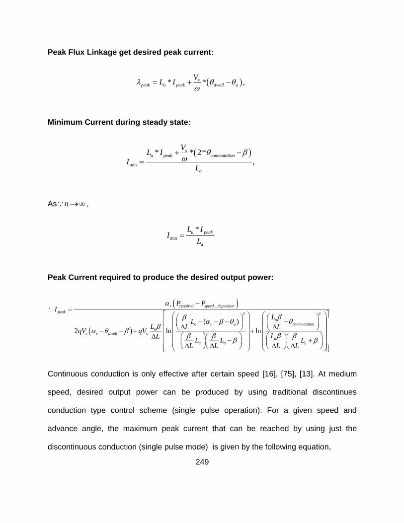
249

Peak Flux Linkage get desired peak current:

* * ,speak u peak dwell a

VL I

Minimum Current during steady state:

min

* * 2*

,

su peak commutation

a

VL I

IL

As n ,

min

*u peak

a

L II

L

Peak Current required to produce the desired output power:

_

22

( )

2 ln ln

r required speed dependant

peak

ucommutationa r a

us r dwell s

ua a u

P PI

LL

L LLqV qV

LLL L L

L L L L

Continuous conduction is only effective after certain speed [16], [75], [13]. At medium

speed, desired output power can be produced by using traditional discontinues

conduction type control scheme (single pulse operation). For a given speed and

advance angle, the maximum peak current that can be reached by using just the

discontinuous conduction (single pulse mode) is given by the following equation,

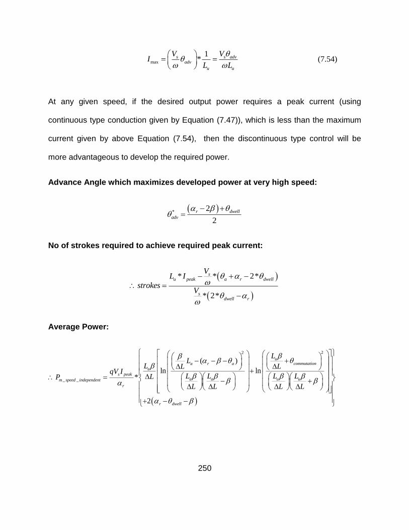
250

max

1*s s adv

adv

u u

V VI

L L

(7.54)

At any given speed, if the desired output power requires a peak current (using

continuous type conduction given by Equation (7.47)), which is less than the maximum

current given by above Equation (7.54), then the discontinuous type control will be

more advantageous to develop the required power.

Advance Angle which maximizes developed power at very high speed:

*2

2

r dwell

adv

No of strokes required to achieve required peak current:

* * 2*

* 2*

su peak a r dwell

sdwell r

VL I

strokesV

Average Power:

22

_ _

( )

ln ln*

2

ucommutationa r a

u

s peaka a u um speed independent

r

r dwell

LL

L LLqV I

L L L LLP

L L L L

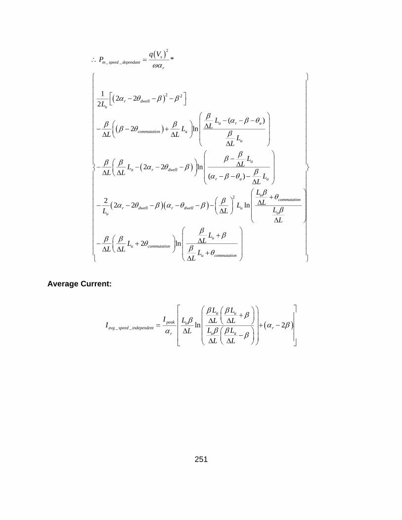
251

2

_ _

2 2

*

12 2

2

( )2 ln

2 2 ln

( )

22 2

s

m speed dependant

r

r dwell

u

a r a

commutation a

a

a

a r dwell

r a a

r dwell r

u

q VP

L

LLL

L LL

L

LLL

L LL

L

L

2

ln

2 ln

ucommutation

dwell uu

u

u commutation

u commutation

L

LLLL

L

LLL

L LL

L

Average Current:

_ _ ln 2

a u

peak uavg speed independent r

u ar

L L

I L L LI

L LL

L L

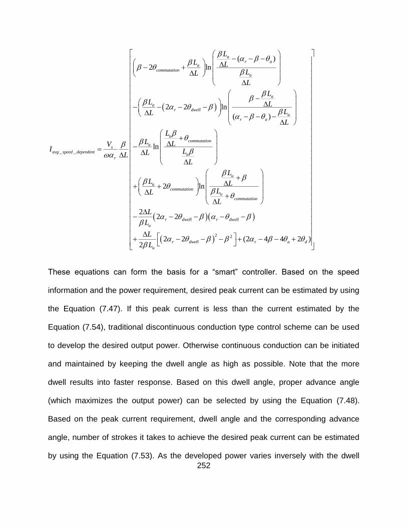
252

_ _

( )2 ln

2 2 ln

( )

ln

2

ar a

acommutation

a

a

ar dwell

ar a

ucommutation

us

avg speed dependentu

r

uco

LL L

LL

L

LL L

LL

L

LL LV

I LLLL

L

L

2 2

ln

22 2

2 2 (2 4 4 2 )2

u

mmutationu

commutation

r dwell r dwell

u

r dwell r a d

u

L

LL

L

L

L

L

L

These equations can form the basis for a “smart” controller. Based on the speed

information and the power requirement, desired peak current can be estimated by using

the Equation (7.47). If this peak current is less than the current estimated by the

Equation (7.54), traditional discontinuous conduction type control scheme can be used

to develop the desired output power. Otherwise continuous conduction can be initiated

and maintained by keeping the dwell angle as high as possible. Note that the more

dwell results into faster response. Based on this dwell angle, proper advance angle

(which maximizes the output power) can be selected by using the Equation (7.48).

Based on the peak current requirement, dwell angle and the corresponding advance

angle, number of strokes it takes to achieve the desired peak current can be estimated

by using the Equation (7.53). As the developed power varies inversely with the dwell

253

angle (Figure 7-26), dwell angle (and the advance angle as it depends on the dwell

angle) can be reduced in smaller steps. Note that the dwell angle has to be more than

half of the rotor pole pitch ( r ) to sustain the continuous conduction.

Next section estimates the maximum speed at which rated power can be developed

using the traditional discontinuous conduction type control scheme (CPSR estimation).

7.4.10 Constant Power Speed Ratio

CPSR is a ratio of the highest speed at which rated power can be developed to the

rated base speed. With discontinuous type conduction, as speed increases, advance

angle and dwell angle have to be increased. At high speed, the SRM operates in single

pulse mode i.e. applied voltage is a square wave. For an 8/6 SRM motor, 30° is the

highest dwell angle that can be applied which guarantees discontinuous type

conduction. So the highest speed, at which rated power that can be developed, by using

traditional discontinuous type conduction, can be found out by doing analysis similar to

continuous conduction analysis described in Section 7.4. Assume a dwell angle is of 30°

and that the motor is operating in a single pulse mode. Figure 7-28 shows resulting

waveforms. Analysis similar to the previous one can be done on these waveforms to

calculate the resultant power. This analysis is based on linear phase inductance

waveform, although saturation can be observed for medium speeds, especially with

high current values. In a single pulse mode, the developed power is given by the

following equation,

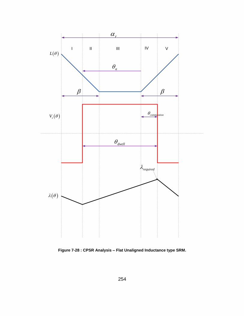
254

required

I II III IV V

a

r

commutation

dwell

L

sV

Figure 7-28 : CPSR Analysis – Flat Unaligned Inductance type SRM.

255

2

*

( ) ln

ln

2 ln

2

sm

r

a

ar a

a

acommutation

aa

a

a

adwell a

acommutation

V qP

L

LL L

LL

L

LL L

LL

L

LL L

LL

L

L

2 2 ( ) 2r r a r

u u

L

L L

(7.55)

This equation can be modified to find the maximum relative speed at which the rated

power that can be developed.

2 30*

( ) ln

ln

2 ln

sCPSR

rated r b

a

ar a

a

acommutation

aa

a

a

adwell a

acommu

V qn

P L N

LL L

LL

L

LL L

LL

L

LL L

LL

L

2 2 ( ) 2

2

tation

r r a r

u u

L L

L L

(7.56)

256

Table 7-7 shows the advance angle dependence of the CPSR. Simulation results (using

a linear model described in Section 7.2.1) confirm that the values predicted by above

equation are the highest speed at which rated power is produced. At relative speed of 6,

with a dwell angle of 30° and advance angle of 24°, linear model simulations predicts

the output power is 325 hp and the above equation predicts the highest relative speed

to be 6.157. With same dwell and advance angle for a relative speed of 6.5, the linear

model simulations predict the output power to be 300 hp. Note that the rated power is

320hp. Next section describes similar analysis on non-flat unaligned inductance type

Switched Reluctance Motors.

7.5 Continuous Conduction Analysis - Non-Flat Unaligned

Inductance

Figure 7-29 shows a different type of per phase inductance profile for a switched

reluctance motor. Note that the unaligned inductance is not flat. During the unaligned

region, inductance continues to decrease but at a smaller rate. Minimum value occurs at

the completely unaligned position. For the example motor, value of the per phase stator

winding inductance at the completely aligned position is 0.07338aL H, inductance value

at the completely unaligned position is 0.004148uL H, and the inductance value at the

on-set of alignment is 0.00524pL H.

257

Table 7-7: CPSR of the Flat Unaligned Inductance type SRM with Discontinuous Conduction.

Advance Angle CPSR Actual Speed (RPM)

15 3.0789 769.725

16 3.4667 866.675

17 3.8469 961.725

18 4.2184 1054.6

19 4.58 1145

20 4.9298 1232.45

21 5.2658 1316.45

22 5.5851 1396.275

23 5.8839 1470.975

24 6.157 1539.25

25 6.3969 1599.225

26 6.5921 1648.025

27 6.724 1681

28 6.7592 1689.8

258

r

L

aL

uL

pL

a pL L L

p uL L L

Figure 7-29 : Non-Flat Unaligned Inductance Profile.

259

Simulation results show that, the balancing zero volt-sec “notch” is symmetrical around

this completely unaligned position.

Figure 7-30 shows the location of the zero volt-sec notch (blue waveform), resultant

phase current (black waveform), resultant flux-linkage (turquoise waveform) and the per

phase inductance (red waveform) profile of an 8/6 SRM motor when operated in

continuous conduction mode.

For analysis purpose, these waveforms can be divided into seven regions. Based on

the applied voltage waveform, the flux-linkage waveform can be derived. Based on the

flux-linkage waveform and the inductance waveform, current waveform can be derived.

Based on this current waveform, developed power can be estimated from the co-energy

area. Figure 7-31 illustrates the same.

Simulation results suggest that the peak current is reached at the completely unaligned

position (i.e. uL L ), while the minimum current occurs at the completely aligned

position (i.e. aL L ). The current regulator set point is reached before the completely

unaligned position ( requiredL L ). This is where the zero volt-second notches starts.

Past this point, current continues to increase but the increase is small.

To keep the consistency with the linear analysis described in the previous section for

flat induction profile type SRM motors, current regulator set point is defined as the peak

current i.e. set peakI I and the actual peak current is defined as _peak newI .

260

Figure 7-30 : Notch Location for Non Flat Unaligned Inductance type SRM when Operated in

Continuous Conduction Mode.

780 790 800 810 820 830 840

-0.06

-0.04

-0.02

0

0.02

0.04

0.06

Angle (Deg)

Applie

d V

oltage(V

olt/1

0000)

and I

nducta

nce(H

)

Applied Voltage and Inductance Vs Angle

261

required

0

I II III I

VV VI VII

r

dwell

adv

commutation

L

sV

sV

sV

aL

uL

pL

minI

peak setI I

_peak newI

i

sV d

iL

Figure 7-31 : Continuous Conduction Analysis – Non Flat Unaligned Inductance type SRM.

262

Now, if Ipeak is the desired peak current set-point, the flux-linkage required to get this

peak current is given by,

*required peak requiredI L (7.57)

Assume that the advance angle ( adv ) and the dwell angle ( dwell ) are given. For an 8/6

SRM motor, the completely unaligned position will be occur at 2

r °. The stabilizing zero

volt-second notch will have a width of 2*2

rdwell

°. Since the current regulator set

point is reached at the end of region 3, value of the phase inductance at this point can

be calculated as below,

,

2

. .

2

p u

r

ru

L LL k

i e

LL L

(7.58)

When5 2 2

r rdwell

,

5 ,p u a pL L L L L L

263

,2

2

2

rrequired u r dwell

rrequired u dwell

rrequired peak u dwell

LL L

LL L

LI L

(7.59)

Region I ends at r adv °. Therefore the width of the first fluxing region can be

calculated as,

,r dwell r adv

adv dwell

commutation

or

We have, 0s

required adv dwell

Vy mx c

0

0

0

,

,2

srequired adv dwell

srequired commutation

srpeak u dwell adv dwell

V

V

VLI L

(7.60)

This is the required value of the residual flux-linkage to achieve desired peak current

set-point. Note that, at high speed, i.e.,

264

0 required

n

Inductance in the region I and II is given by6,

,

( ) * ,

y mx c

LL k

When, 0 , ( ) aL L . When , ( ) ,pL L therefore,

( ) ,

( )

a

a

LLL

L

LL L

(7.61)

7.5.1 Region I Analysis ( 0 ( )r adv )

Flux Linkages in the region I is given by,

( ) ( 2 2 ),

( ) ( 2 2 )

s srequired r adv dwell

srequired r adv dwell

V V

V

(7.62)

And

( ) sVd d

(7.63)

Current in the region I is given by,

6 k = arbitrary constant.

265

( )( )

( )

( 2 2 )

( )

srequired r adv dwell

a

IL

V

ILL

L

(7.64)

Power produced in the region I is given by,

( )

1

0

( )

1

0

( )* ( )

( 2 2 )

*

r a

r as

required r adv dwells

a

P i d

VV

P dLL

L

2

1

2

ln

2 2 ln

aadv r

s srequired r adv

a

aadv r

s aadv r dwell

a

LV VLP

LL L

L

LV L L

LL L

L

(7.65)

Flux Linkage in the regions II and III is given by,

( ) srequired r dwell

V

(7.66)

And

( ) sVd d

(7.67)

When, ( ),r adv

266

0

( ) * ( )

*

*

*

srequired r dwell r adv

srequired dwell adv

srequired dwell adv

srequired commutation

V

V

V

V

(Verification)

7.5.2 Region II Analysis ( ( )r adv )

Current in the region II is given by,

( )

srequired r dwell

a

V

ILL

L

(7.68)

Power produced in region II is given by,

2

( )

2

( )

2

2

( ) ( )

( ) ( )

1

r a

r adv

r adv r adv

srequired r dwell

s

a

r dwells srequired

a a

P i d

VV

P dLL

L

V VP d d

L LL L

L L

267

2

2

2

ln 2

ln

p

s srequired r adv

aadv r

p

s adwell r

aadv r

L

V VLPLL L

L

L

V L LLL L

L

(7.69)

7.5.3 Region III Analysis ( r dwell )

Inductance in this region and the region IV-a is given by,

2

ru

LL L

(7.70)

Current in the region III is given by,

( ) ,

2

srequired r dwell

u r

V

ILL

L

(7.71)

Power produced in the region III is given by,

3

3

,

2

2

r dwell

r dwell

srequired r dwell

s

u r

srequired r dwell

s

u r

VV

P dLL

L

VV

P dLL

L

268

2

3

2

2ln

2

2ln2

2

u rdwell

s srequired r dwell

u r

u rdwell

s u rdwell

u r

LV VLP

LL L

L

LV L L

LL L

L

(7.72)

7.5.4 Region IV-a Analysis ( 2

rr dwell

)

Flux linkage in the region IV-a is given by,

( ) required (7.73)

And

( ) 0d (7.74)

Current in region IV-a is given by,

( )

2

required

ru

IL

L

(7.75)

At the beginning of this region current reaches the desired peak value. In this region,

phase current continuous to grow. Current reaches a new peak value at the end of this

section.

_

_

2r

peak desired u dwellrequired

peak new

u u

LI L

IL L

(7.76)

Power produced in this region is zero as 0d

d

.

269

Inductance in the regions IV-b and V is given by,

( )2

ru

LL L

(7.77)

When r ,

( ) ,2

( )2

ru r

ru p

LL L

LL L L

(Verification)

7.5.5 Region IV-b Analysis (2

rdwell

)

Flux linkage in the region IV-b is given by,

( ) required (7.78)

And

( ) 0d (7.79)

Current in the region IV-b is given by,

( )

2

required

ru

IL

L

(7.80)

Power produced in this region zero i.e.

4

( ) ( )* ( ) 0dwell

r dwell

P i d

Flux linkage in the regions V and VI is given by,

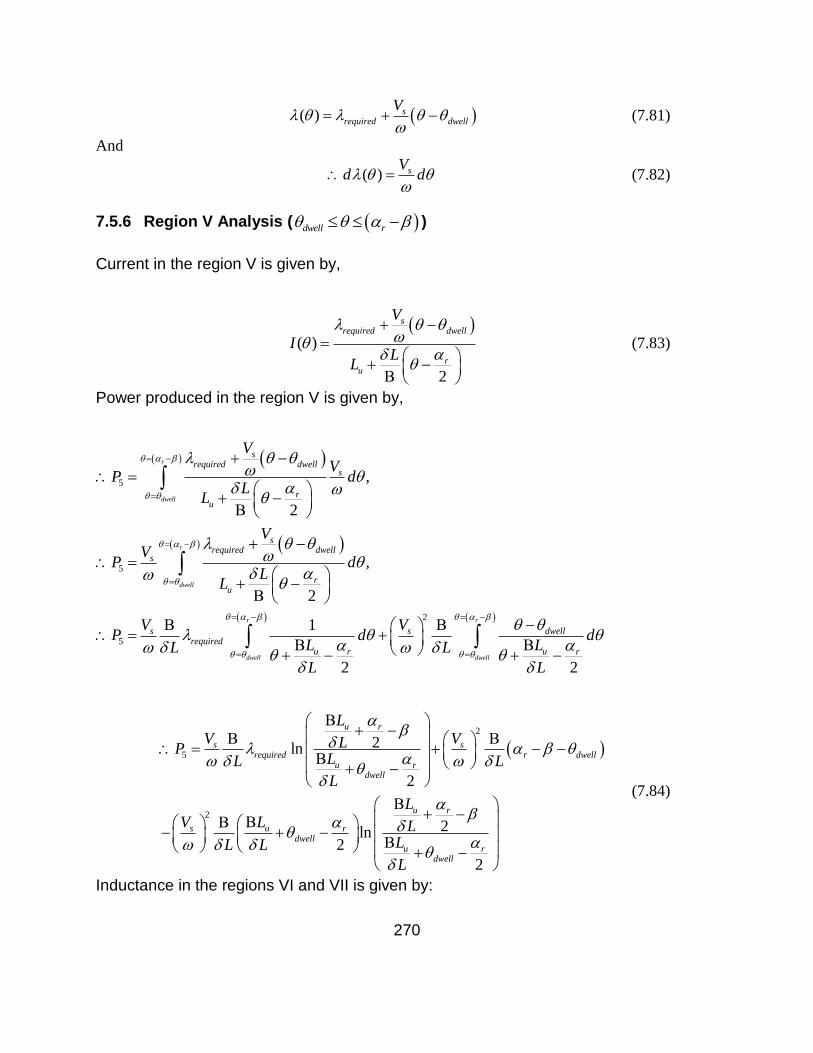
270

( ) srequired dwell

V

(7.81)

And

( ) sVd d

(7.82)

7.5.6 Region V Analysis ( dwell r )

Current in the region V is given by,

( )

2

srequired dwell

ru

V

IL

L

(7.83)

Power produced in the region V is given by,

5

5

2

5

,

2

,

2

1

2

r

dwell

r

dwell

r

dwell

srequired dwell

s

ru

srequired dwell

s

ru

s s dwellrequired

u r

VV

P dL

L

VV

P dL

L

V VP d

L LL L

L

2

r

dwellu r

d

L

2

5

2

2ln

2

2ln2

2

u r

s srequired r dwell

u rdwell

u r

s u rdwell

u rdwell

LV VLP

LL L

L

LV L L

LL L

L

(7.84)

Inductance in the regions VI and VII is given by:

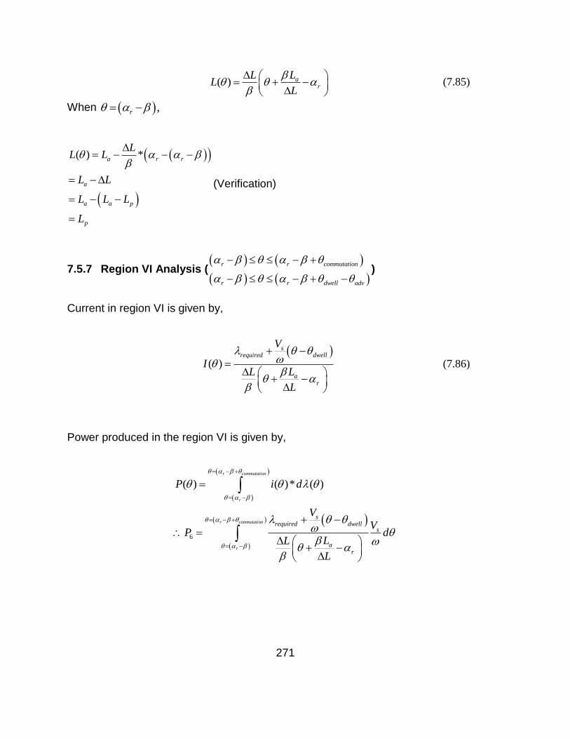
271

( ) ar

LLL

L

(7.85)

When ,r

( ) *a r r

a

a a p

p

LL L

L L

L L L

L

(Verification)

7.5.7 Region VI Analysis (

r r commutation

r r dwell adv

)

Current in region VI is given by,

( )

srequired dwell

ar

V

ILL

L

(7.86)

Power produced in the region VI is given by,

6

( ) ( )* ( )r commutation

r

r commutation

r

srequired dwell

s

ar

P i d

VV

P dLL

L

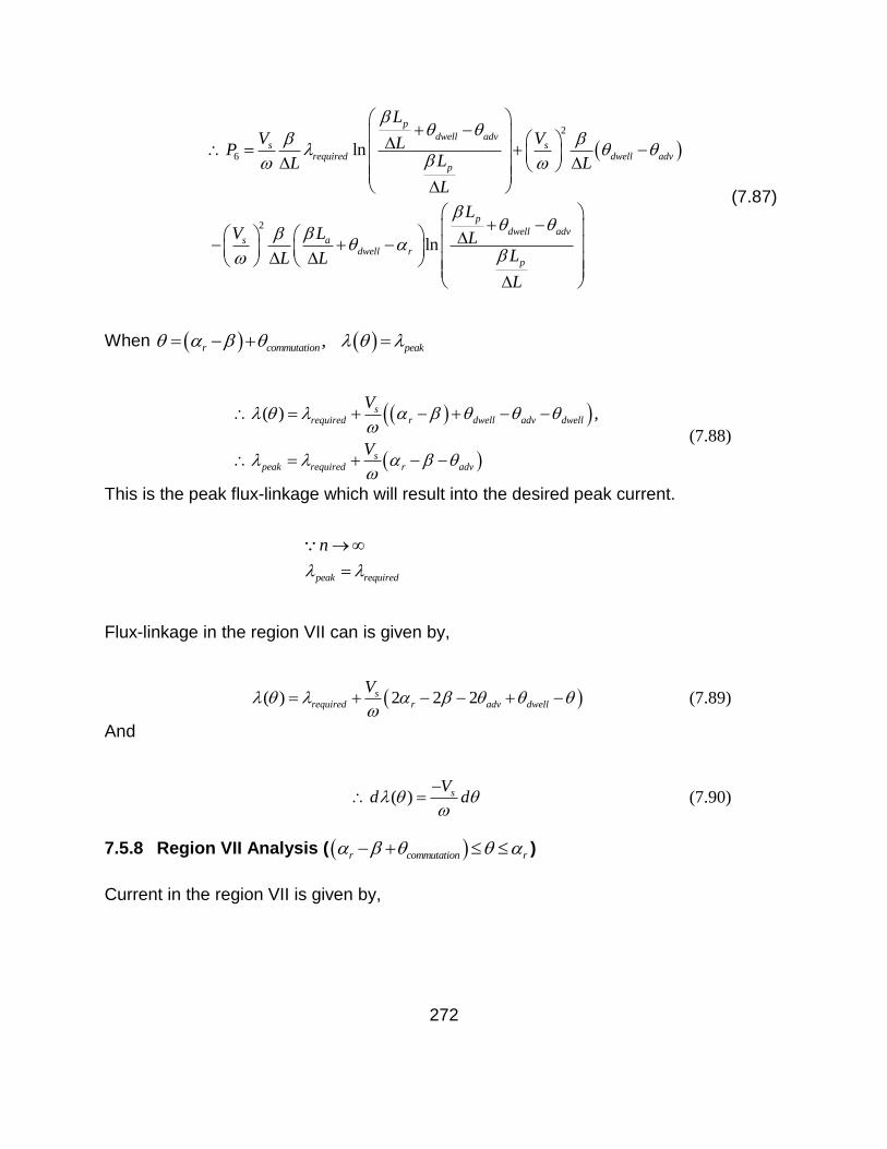
272

2

6

2

ln

ln

p

dwell advs s

required dwell advp

p

dwell advs a

dwell rp

L

V VLPLL L

L

L

V L LLL L

L

(7.87)

When ,r commutation peak

( ) ,srequired r dwell adv dwell

speak required r adv

V

V

(7.88)

This is the peak flux-linkage which will result into the desired peak current.

peak required

n

Flux-linkage in the region VII can is given by,

( ) 2 2 2srequired r adv dwell

V

(7.89)

And

( ) sVd d

(7.90)

7.5.8 Region VII Analysis ( r commutation r )

Current in the region VII is given by,

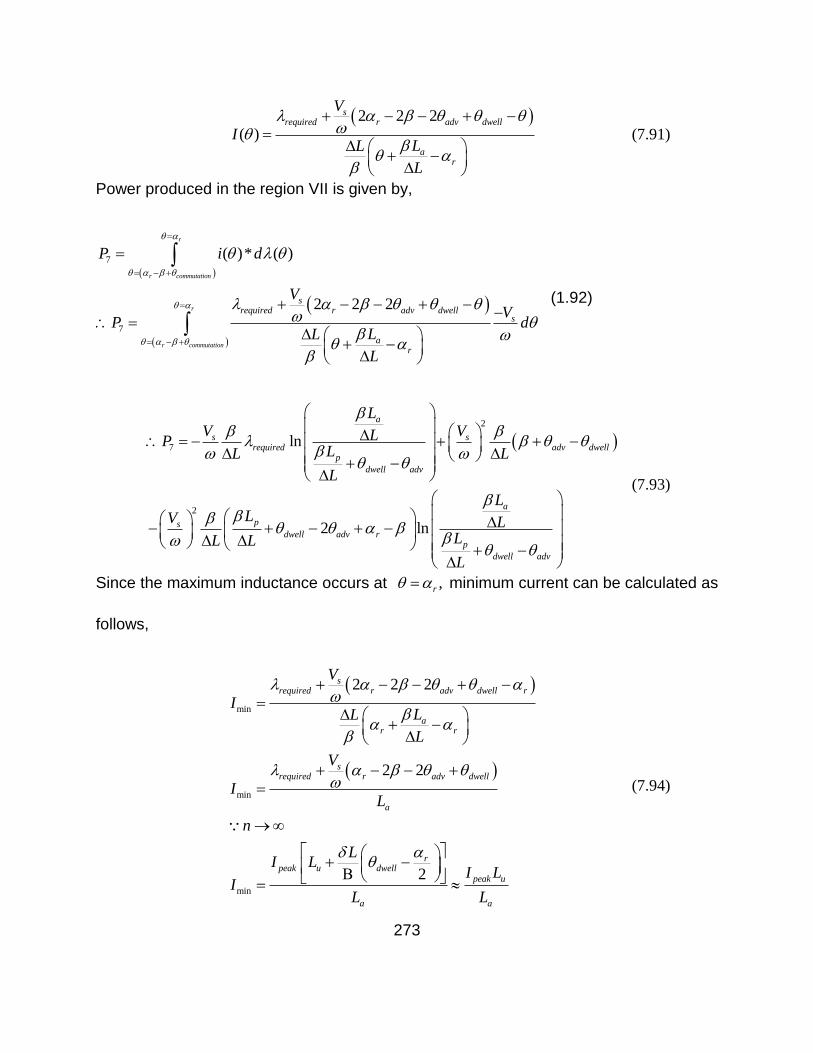
273

2 2 2

( )

srequired r adv dwell

ar

V

ILL

L

(7.91)

Power produced in the region VII is given by,

7

7

( )* ( )

2 2 2

r

r commutation

r

r commutation

srequired r adv dwell

s

ar

P i d

VV

P dLL

L

(1.92)

2

7

2

ln

2 ln

a

s srequired adv dwell

p

dwell adv

a

psdwell adv r

p

dwell adv

LV VLP

LL L

L

LLV L

LL L

L

(7.93)

Since the maximum inductance occurs at ,r minimum current can be calculated as

follows,

min

min

min

2 2 2

2 2

2

srequired r adv dwell r

ar r

srequired r adv dwell

a

rpeak u dwell

peak u

a a

V

ILL

L

V

IL

n

LI L

I LI

L L

(7.94)

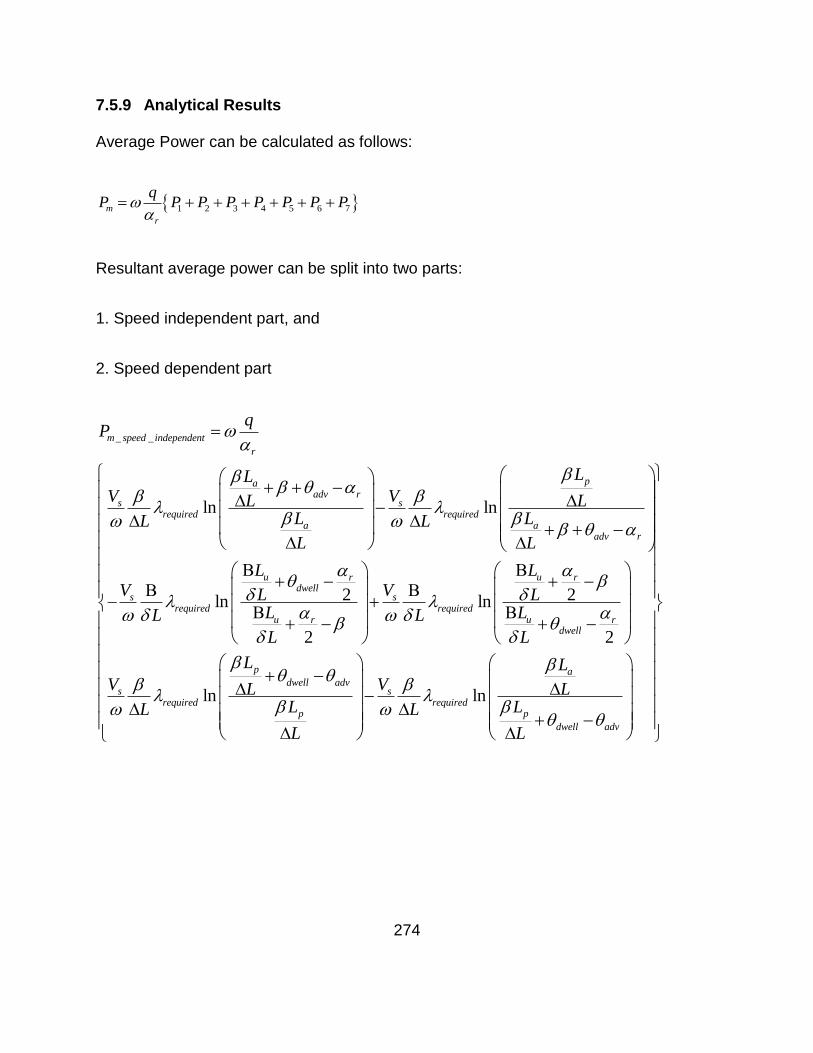
274

7.5.9 Analytical Results

Average Power can be calculated as follows:

1 2 3 4 5 6 7m

r

qP P P P P P P P

Resultant average power can be split into two parts:

1. Speed independent part, and

2. Speed dependent part

_ _

ln ln

2ln ln

2

m speed independent

r

paadv r

s srequired required

a aadv r

u urdwell

s srequired required

u r

qP

LLV VL L

L LL L

L L

L LV VL L

LL L

L

2

2

ln ln

r

u rdwell

p adwell adv

s srequired required

p p

dwell adv

L

L

L LV VL L

L LL L

L L

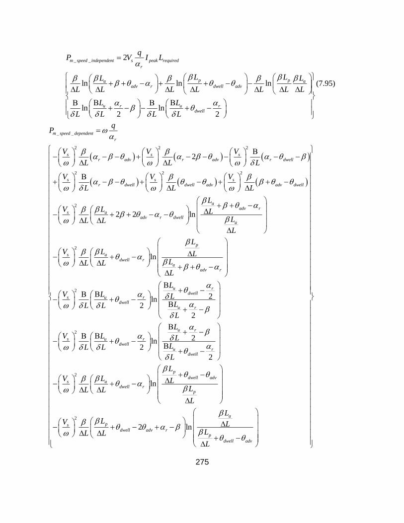
275

_ _ 2

ln ln ln

ln ln2 2

m speed independent s peak required

r

p pa aadv r dwell adv

u ur rdwell

qP V I L

L LL L

L L L L L L L

L L

L L L L

(7.95)

_ _

2 2 2

2 2 2

2

2

2 2

m speed dependent

r

s s sr adv r adv r dwell

s s sr dwell dwell adv adv dwell

s aadv

qP

V V V

L L L

V V V

L L L

V L

L L

2

2

ln

ln

2ln2

2

aadv r

r dwella

p

s adwell r

aadv r

u rdwell

s u rdwell

u r

s

L

LL

L

L

V L LLL L

L

LV L L

LL L

L

V

2

2

2

2ln2

2

ln

2 ln

u r

u rdwell

u rdwell

p

dwell advs a

dwell rp

a

psdwell adv r

p

dwell

LL L

LL L

L

L

V L LLL L

L

LLV L

LL L

L

adv

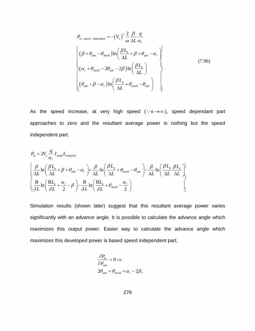
276

2

_ _

2

ln

2 2 ln

ln

m speed dependant s

r

aadv dwell adv r

ar dwell adv

p

adv r dwell adv

qP V

L

L

L

L

L

L

L

(7.96)

As the speed increase, at very high speed ( n ), speed dependant part

approaches to zero and the resultant average power is nothing but the speed

independent part.

2

ln ln ln

ln ln2 2

m s peak required

r

p pa aadv r dwell adv

u ur rdwell

qP V I L

L LL L

L L L L L L L

L L

L L L L

Simulation results (shown later) suggest that this resultant average power varies

significantly with an advance angle. It is possible to calculate the advance angle which

maximizes this output power. Easier way to calculate the advance angle which

maximizes this developed power is based speed independent part.

0

2 2 ,

m

adv

adv dwell r

P

277

*

*

2

2

2 2

dwell radv

dwell radv

or

(7.97)

Note that this power maximizing advance angle only depends on the dwell angle and

machine design parameters. Number of strokes required to achieve the desired peak

current is calculated next. Initially during each stroke, since dwell angle is more than

half of the rotor pole pitch, the fluxing region will be more than the de-fluxing region.

Therefore at the end of each stroke, initial flux linkage will increase by,

* 2* ,sadd dwell r

V

Since 0 ,srequired dwell adv

V

2 ,

2

s sdwell r required dwell adv

srequired dwell adv

sdwell r

V Vstrokes

V

strokesV

(7.98)

As described in the previous section, a better way to control the output power is by the

peak current set-point. Developed power also depends on the advance angle and the

dwell angle, but by making the output power proportional to the phase current, better

partial load efficiency can be achieved (as good as the full load efficiency). The speed

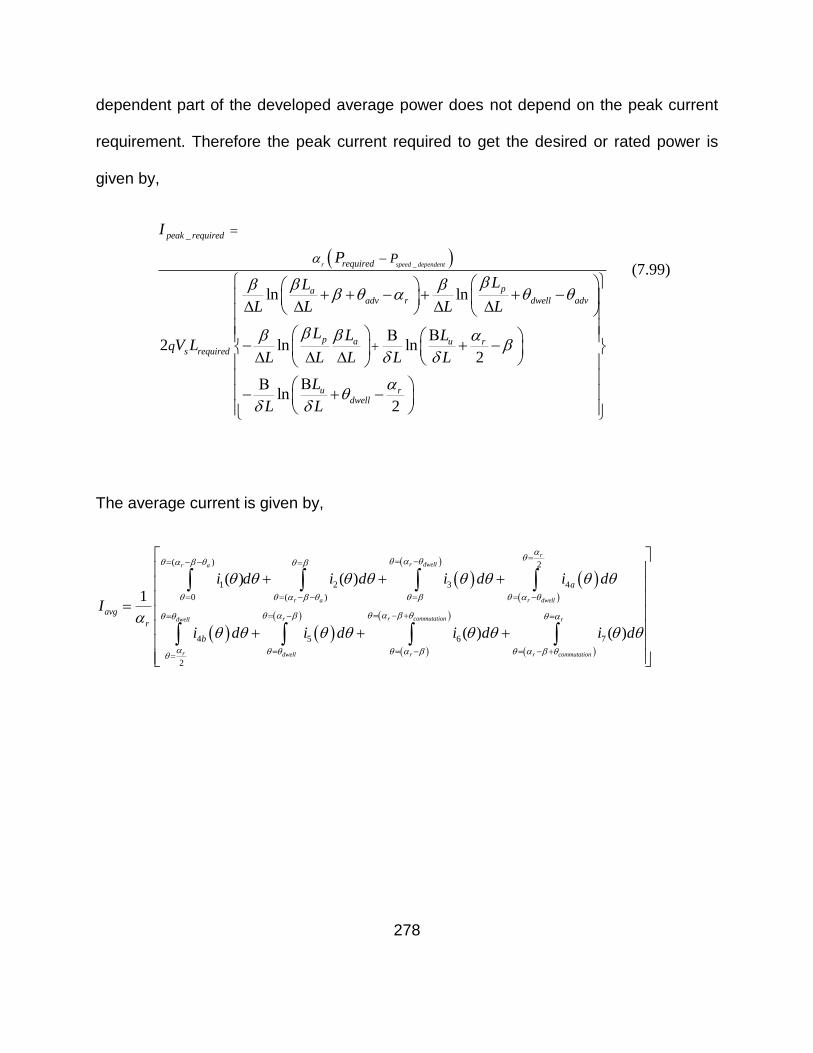
278

dependent part of the developed average power does not depend on the peak current

requirement. Therefore the peak current required to get the desired or rated power is

given by,

_

_

ln ln

2 ln ln2

ln2

r speed dependent

peak required

required

paadv r dwell adv

p a u rs required

u rdwell

P

q

I

P

LL

L L L L

L L LV L

L L L L L

L

L L

(7.99)

The average current is given by,

( ) 2

1 2 3 4

0 ( )

4 5 6 7

2

( ) ( )1

( ) ( )

r

r dwellr a

r a r dwell

r commutationrdwell

r dwell r r commutation

a

avg

r

b

i d i d i d i d

I

i d i d i d i d

r

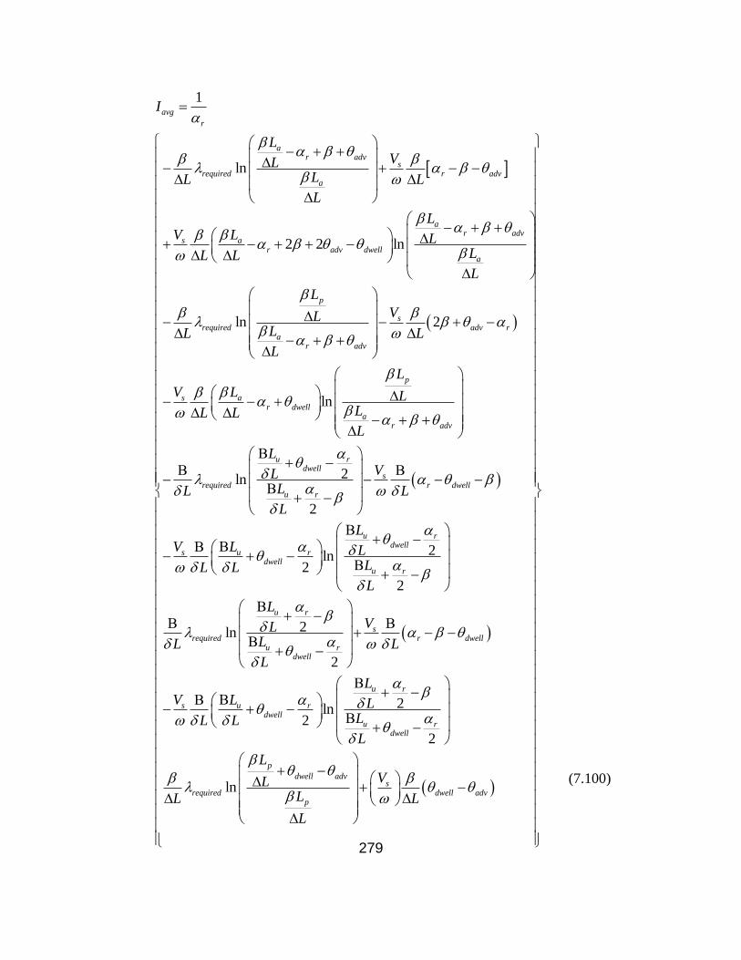
279

1

ln

2 2 ln

ln 2

avg

r

ar adv

srequired r adv

a

ar adv

s ar adv dwell

a

p

srequired adv

ar adv

I

LVL

LL L

L

LV L L

LL L

L

L

VLLL L

L

ln

2ln

2

2ln2

2

r

p

s ar dwell

ar adv

u rdwell

srequired r dwell

u r

u rdwell

s u rdwell

u r

L

V L LLL L

L

LVL

LL L

L

LV L L

LL L

L

2ln

2

2ln2

2

ln

u r

srequired r dwell

u rdwell

u r

s u rdwell

u rdwell

p

dwell advs

requiredp

LVL

LL L

L

LV L L

LL L

L

L

VLLL L

L

dwell adv

(7.100)

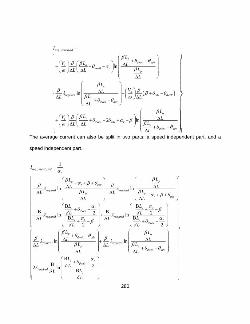
280

_

ln

ln

2

avg continued

p

dwell advs a

dwell rp

a

srequired adv dwell

p

dwell adv

psdwell adv r

I

L

V L LLL L

L

LVL

LL L

L

LV

L L

ln

a

p

dwell adv

L

LL

L

The average current can also be split in two parts: a speed independent part, and a

speed independent part.

_ _

1

ln ln

2 2ln ln

2

avg speed ind

r

par adv

required requireda a

r adv

u ur rdwell

required requiredu ur

dwell

I

LL

L LL LL L

L L

L L

L LL LL L

L L

2

ln ln

22 ln

r

p adwell adv

required requiredp p

dwell adv

u rdwell

requiredu

L L

L LL LL L

L L

L

LLL

L

281

_ _ 2

2ln ln

required

avg speed ind

r

u r

a

up

I

LL L

LL L L

L

(7.101)

_ _ 2

2ln ln

peak required

avg speed ind

r

u r

a

up

I LI

LL L

LL L L

L

This is the dominant part of the total average current. Note that this part does not

depend on the choice of dwell angle or the advance angle. It only depends on the peak

current.

_ _

1

2 2 2 1 ln

2 ln

2 2 ln

savg speed dependant

r

ar dwell adv

a ar adv r adv

p padwell adv dwell adv

VI

L

L

L

L L

L L

L LL

L L L

(7.102)

282

Simulation results suggest that the combination of the advance angle and the dwell

angle which makes this speed dependant part zero, produces the maximum power per

amp. In general, we have,

Required Flux Linkage to get Desired Peak Current:

* ,

2

required peak required

rrequired peak u dwell

I L

LI L

Required Residual Flux Linkage to get desired Peak Current:

0 ,srequired adv dwell

V

Required Peak Flux Linkage to get desired Peak Current:

speak required r adv

V

Resultant Minimum Current:

min

min

2 2

2

srequired r adv dwell

a

rpeak u dwell

peak u

a a

V

IL

n

LI L

I LI

L L

Advance Angle which maximizes the developed power at very high speed:

283

*

2 2

dwell radv

No of strokes required to achieve the desired peak current:

2

srequired dwell adv

sdwell r

V

strokesV

Resultant Average Power:

_ _ 2

ln ln ln

ln ln2 2

m speed independent s peak required

r

p pa aadv r dwell adv

u ur rdwell

qP V I L

L LL L

L L L L L L L

L L

L L L L

2

_ _

2

ln

2 2 ln

ln

m speed dependant s

r

aadv dwell adv r

ar dwell adv

p

adv r dwell adv

qP V

L

L

L

L

L

L

L

Resultant Average Current:

284

_ _ 2

2ln ln

required

avg speed ind

r

u r

a

up

I

LL L

LL L L

L

_ _

1

2 2 2 1 ln

2 ln

2 2 ln

s

avg speed dependant

r

a

r dwell adv

a a

r adv r adv

p pa

dwell adv dwell adv

VI

L

L

L

L L

L L

L LL

L L L

Peak Current required to get the desired Power,

_

_

ln ln

2 ln ln2

ln2

r speed dependant

peak required

required

paadv r dwell adv

p a u rs required

u rdwell

P

q

I

P

LL

L L L L

L L LV L

L L L L L

L

L L

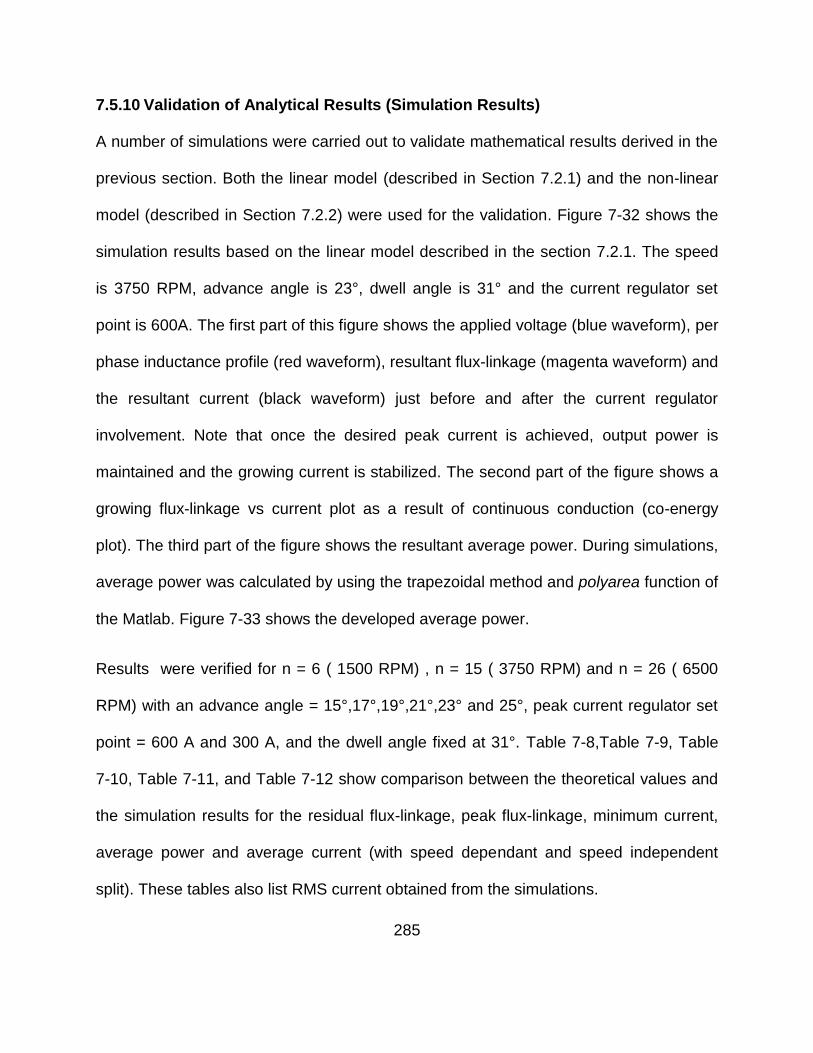
285

7.5.10 Validation of Analytical Results (Simulation Results)

A number of simulations were carried out to validate mathematical results derived in the

previous section. Both the linear model (described in Section 7.2.1) and the non-linear

model (described in Section 7.2.2) were used for the validation. Figure 7-32 shows the

simulation results based on the linear model described in the section 7.2.1. The speed

is 3750 RPM, advance angle is 23°, dwell angle is 31° and the current regulator set

point is 600A. The first part of this figure shows the applied voltage (blue waveform), per

phase inductance profile (red waveform), resultant flux-linkage (magenta waveform) and

the resultant current (black waveform) just before and after the current regulator

involvement. Note that once the desired peak current is achieved, output power is

maintained and the growing current is stabilized. The second part of the figure shows a

growing flux-linkage vs current plot as a result of continuous conduction (co-energy

plot). The third part of the figure shows the resultant average power. During simulations,

average power was calculated by using the trapezoidal method and polyarea function of

the Matlab. Figure 7-33 shows the developed average power.

Results were verified for n = 6 ( 1500 RPM) , n = 15 ( 3750 RPM) and n = 26 ( 6500

RPM) with an advance angle = 15°,17°,19°,21°,23° and 25°, peak current regulator set

point = 600 A and 300 A, and the dwell angle fixed at 31°. Table 7-8,Table 7-9, Table

7-10, Table 7-11, and Table 7-12 show comparison between the theoretical values and

the simulation results for the residual flux-linkage, peak flux-linkage, minimum current,

average power and average current (with speed dependant and speed independent

split). These tables also list RMS current obtained from the simulations.

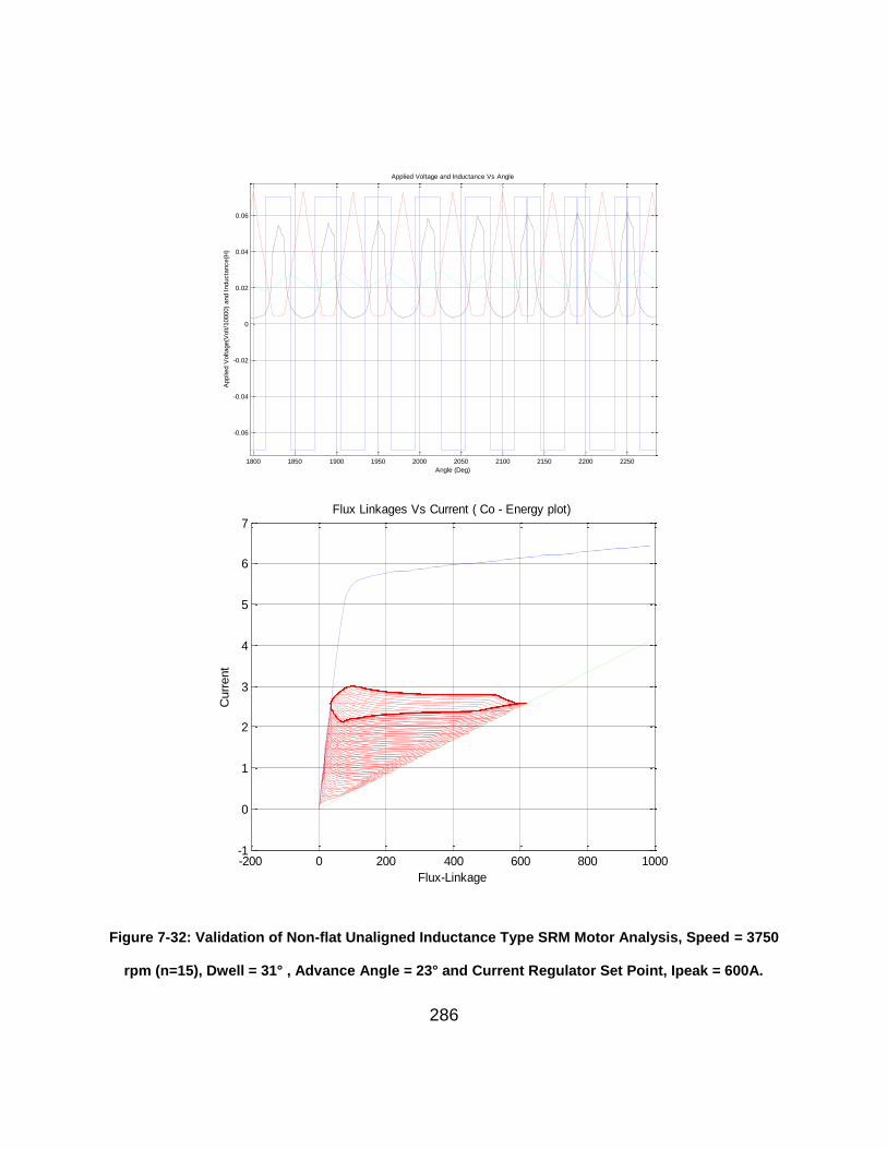
286

Figure 7-32: Validation of Non-flat Unaligned Inductance Type SRM Motor Analysis, Speed = 3750

rpm (n=15), Dwell = 31° , Advance Angle = 23° and Current Regulator Set Point, Ipeak = 600A.

1800 1850 1900 1950 2000 2050 2100 2150 2200 2250

-0.06

-0.04

-0.02

0

0.02

0.04

0.06

Angle (Deg)

Applie

d V

oltage(V

olt/1

0000)

and I

nducta

nce(H

)

Applied Voltage and Inductance Vs Angle

-200 0 200 400 600 800 1000-1

0

1

2

3

4

5

6

7

Flux-Linkage

Curr

ent

Flux Linkages Vs Current ( Co - Energy plot)

287

Figure 7-33 : Average Power.

0 20 40 60 80 100 120100

150

200

250

300

350

400

450

500

550

600

X: 73

Y: 524.6

Cycles

Pow

er

(HP

)

Average Power per Cycle

288

Table 7-8 : Non-flat Unaligned Inductance type SRM, Dwell = 31° (Linear Model and Non Linear Model).

Sim.

Result

Theor.

Result

Sim.

Result

Theore

tical

Sim.

Result

Theore

tical

Sim.

Result

Theore

tical

Speed.

Ind.

Speed

Dep.

Sim.

Result

Theor.

Result

Speed

Ind.

Speed

Dep.

15 2.0538 2.0711 4.3115 4.3266 51.905 52.073 441.68 440.01 407.49 32.525 225.97 227.13 212.6 14.527 303.71

17 1.9012 1.9155 4.1571 4.1711 47.688 47.833 499.52 499.1 476.46 22.639 221.66 222.71 212.6 10.115 302.24

19 1.7449 1.76 4.0019 4.0155 43.418 43.593 523.8 522.54 507.66 14.877 217.98 219.05 212.6 6.4516 301.3

21 1.5908 1.6044 3.8461 3.86 39.191 39.353 530.4 530.19 522.77 7.4242 214.74 215.75 212.6 3.1485 300.72

23 1.4381 1.4489 3.6926 3.7044 34.966 35.114 527.21 527.36 527.36 0 211.72 212.6 212.6 0 300.3

25 1.279 1.2933 3.5357 3.5489 30.687 30.874 516.06 515.34 522.77 -7.424 208.34 209.45 212.6 -3.149 299.37

15 2.058 2.0711 4.3171 4.3266 53.821 52.073 615.97 440.01 407.49 32.525 318.39 227.13 212.6 14.527 378.13

17 1.9062 1.9155 4.1629 4.1711 48.926 47.833 701.48 499.1 476.46 22.639 303.52 222.71 212.6 10.115 370.79

19 1.7498 1.76 4.0076 4.0155 44.333 43.593 728.15 522.54 507.66 14.877 291.08 219.05 212.6 6.4516 365.57

21 1.5966 1.6044 3.8535 3.86 39.855 39.353 697.74 530.19 522.77 7.4242 281.42 215.75 212.6 3.1485 361.31

23 1.4443 1.4489 3.7002 3.7044 35.419 35.114 639.84 527.36 527.36 0 272.1 212.6 212.6 0 356.19

25 1.2872 1.2933 3.5458 3.5489 31.016 30.874 570.11 515.34 522.77 -7.424 261.82 209.45 212.6 -3.149 349.51

Speed = 1500 RPM , Peak Current = 600 A Non Linear Model

Average

Current (A)

Speed = 1500 RPM , Peak Current = 600 A Linear Model

Intial Flux

Linkage (Wb)Adv.

Angle

Peak Flux

Linkage (Wb)

Minimum

Current (A)

Average Power

(HP)

RMS

Cur.

Average

Current (A)

Average Power

(HP)

289

Table 7-9 : Non-flat Unaligned Inductance type SRM Dwell = 31° (Linear Model).

Sim.

Result

Theor.

Result

Sim.

Result

Theor.

Result

Sim.

Result

Theor.

Result

Sim.

Result

Theor.

Result

Speed

Ind.

Speed

Dep.

Sim.

Result

Theor.

Result

Speed

Ind.

Speed

Dep.

15 2.3626 2.3744 3.2639 3.2766 41.831 41.897 422.22 420.5 407.49 13.01 217.44 218.41 212.6 5.8107 299.39

17 2.3044 2.3122 3.2048 3.2144 40.193 40.201 485.55 485.51 476.46 9.0556 215.98 216.65 212.6 4.0458 299.1

19 2.2363 2.25 3.1378 3.1522 38.415 38.505 514.92 513.61 507.66 5.9508 214.07 215.18 212.6 2.5806 298.09

21 2.1759 2.1878 3.0769 3.09 36.716 36.81 526.5 525.73 522.77 2.9697 212.91 213.86 212.6 1.2594 298.05

23 2.1166 2.1255 3.0166 3.0278 35.053 35.114 526.4 527.36 527.36 0 211.81 212.6 212.6 0 298.02

25 2.0529 2.0633 2.9539 2.9655 33.336 33.418 520.98 519.8 522.77 -2.97 210.38 211.34 212.6 -1.259 297.57

15 1.0827 1.0861 1.9833 1.9883 24.323 24.34 217.16 216.75 203.74 13.01 111.8 112.11 106.3 5.8107 151.36

17 1.0221 1.0239 1.9218 1.9261 22.646 22.645 246.77 247.28 238.23 9.0556 110.13 110.35 106.3 4.0458 150.82

19 0.9573 0.9617 1.8587 1.8639 20.912 20.949 260.49 259.78 253.83 5.9508 108.5 108.88 106.3 2.5806 150.24

21 0.8959 0.8994 1.7965 1.8017 19.218 19.253 264.46 264.35 261.38 2.9697 107.25 107.56 106.3 1.2594 150.05

23 0.8367 0.8372 1.7359 1.7394 17.551 17.557 263 263.68 263.68 0 106.14 106.3 106.3 0 150.02

25 0.7713 0.775 1.6726 1.6772 15.819 15.861 258.95 258.41 261.38 -2.97 104.71 105.04 106.3 -1.259 149.54

Average

Power (HP) RMS

Cur.

(A)

Average

Current (A)

Average

Power (HP)

Average

Current (A)

Speed = 3750 RPM , Peak Current = 600 A

Speed = 3750 RPM , Peak Current = 300 A

Intial Flux

Linkage (Wb)Adv.

Angle

Peak Flux

Linkage (Wb)

Minimum

Current (A)

290

Table 7-10: Non-flat Unaligned Inductance type SRM Dwell = 31° (Non Linear Model).

Sim.

Result

Theor.

Result

Sim.

Result

Theor.

Result

Sim.

Result

Theor.

Result

Sim.

Result

Theor.

Result

Speed

Ind.

Speed

Dep.

Sim.

Result

Theor.

Result

Speed

Ind.

Speed

Dep.

15 2.3705 2.3744 3.2726 3.2766 42.677 41.897 467.97 420.5 407.49 13.01 273.8 218.41 212.6 5.8107 342.79

17 2.3141 2.3122 3.215 3.2144 40.964 40.201 570.65 485.51 476.46 9.0556 269.55 216.65 212.6 4.0458 340.38

19 2.2455 2.25 3.1473 3.1522 39.08 38.505 645.83 513.61 507.66 5.9508 264.75 215.18 212.6 2.5806 337.49

21 2.1856 2.1878 3.0863 3.09 37.314 36.81 678.79 525.73 522.77 2.9697 261.76 213.86 212.6 1.2594 336.66

23 2.1267 2.1255 3.0268 3.0278 35.568 35.114 660.78 527.36 527.36 0 259.13 212.6 212.6 0 336.03

25 2.0591 2.0633 2.9613 2.9655 33.734 33.418 612.52 519.8 522.77 -2.97 255.39 211.34 212.6 -1.259 333.97

15 1.0883 1.0861 1.9891 1.9883 24.495 24.34 229.01 216.75 203.74 13.01 118.41 112.11 106.3 5.8107 157.33

17 1.0275 1.0239 1.9277 1.9261 22.784 22.645 266.18 247.28 238.23 9.0556 116.16 110.35 106.3 4.0458 156.34

19 0.9636 0.9617 1.8648 1.8639 21.05 20.949 281.56 259.78 253.83 5.9508 114.51 108.88 106.3 2.5806 155.82

21 0.9019 0.8994 1.8023 1.8017 19.33 19.253 285.73 264.35 261.38 2.9697 113.17 107.56 106.3 1.2594 155.59

23 0.8427 0.8372 1.7419 1.7394 17.64 17.557 283.93 263.68 263.68 0 112.05 106.3 106.3 0 155.57

25 0.7766 0.775 1.6776 1.6772 16.141 15.861 278.61 258.41 261.38 -2.97 110.45 105.04 106.3 -1.259 154.96

Speed = 3750 RPM , Peak Current = 600 A

Speed = 3750 RPM , Peak Current = 300 A

Intial Flux

Linkage (Wb)Adv.

Angle

Peak Flux

Linkage (Wb)

Minimum

Current (A)

Average

Power (HP)

RMS

Cur.

Average

Current (A)

Average

Power (HP)

Average

Current (A)

291

Table 7-11 : Non-flat Unaligned Inductance type SRM Dwell = 31° (Linear Model).

Sim.

Result

Theor.

Result

Sim.

Result

Theor.

Result

Sim.

Result

Theor.

Result

Sim.

Result

Theor.

Result

Speed

Ind.

Speed

Dep.

Sim.

Result

Theor.

Result

Speed

Ind.

Speed

Dep.

15 2.4473 2.46 2.9662 2.9805 39.043 39.027 415.28 414.99 407.49 7.5058 214.91 215.95 212.6 3.3523 298.27

17 2.4133 2.4241 2.9319 2.9446 38.038 38.049 481.24 481.68 476.46 5.2244 213.91 214.93 212.6 2.3341 297.97

19 2.3782 2.3882 2.8971 2.9087 37.072 37.071 512.09 511.09 507.66 3.4331 213.14 214.09 212.6 1.4888 297.84

21 2.3435 2.3523 2.8621 2.8728 36.108 36.092 525.01 524.48 522.77 1.7133 212.46 213.33 212.6 0.7266 297.8

23 2.3073 2.3164 2.826 2.8369 35.135 35.114 527.5 527.36 527.36 0 211.82 212.6 212.6 0 297.72

25 2.2677 2.2805 2.7868 2.801 34.105 34.135 522.21 521.05 522.77 -1.713 210.68 211.87 212.6 -0.727 297.05

15 1.171 1.1717 1.6892 1.6922 21.521 21.47 211.53 211.25 203.74 7.5058 109.5 109.65 106.3 3.3523 150.37

17 1.1341 1.1358 1.6527 1.6563 20.531 20.492 243.69 243.45 238.23 5.2244 108.45 108.63 106.3 2.3341 149.9

19 1.0966 1.0999 1.6151 1.6204 19.518 19.514 257.26 257.26 253.83 3.4331 107.42 107.79 106.3 1.4888 149.44

21 1.0609 1.064 1.5798 1.5845 18.56 18.535 263.53 263.1 261.38 1.7133 106.74 107.03 106.3 0.7266 149.38

23 1.0262 1.0281 1.5442 1.5486 17.583 17.557 263.29 263.68 263.68 0 106.02 106.3 106.3 0 149.27

25 0.9897 0.9922 1.5082 1.5127 16.603 16.578 259.68 259.67 261.38 -1.713 105.31 105.57 106.3 -0.727 149.12

Speed = 6500 RPM , Peak Current = 300 A

Intial Flux

Linkage (Wb)Adv.

Angle

Peak Flux

Linkage (Wb)

Minimum

Current (A)

Average

Power (HP) RMS

Cur.

(A)

Average

Current (A)

Average

Power (HP)

Average

Current (A)

Speed = 6500 RPM , Peak Current = 600 A

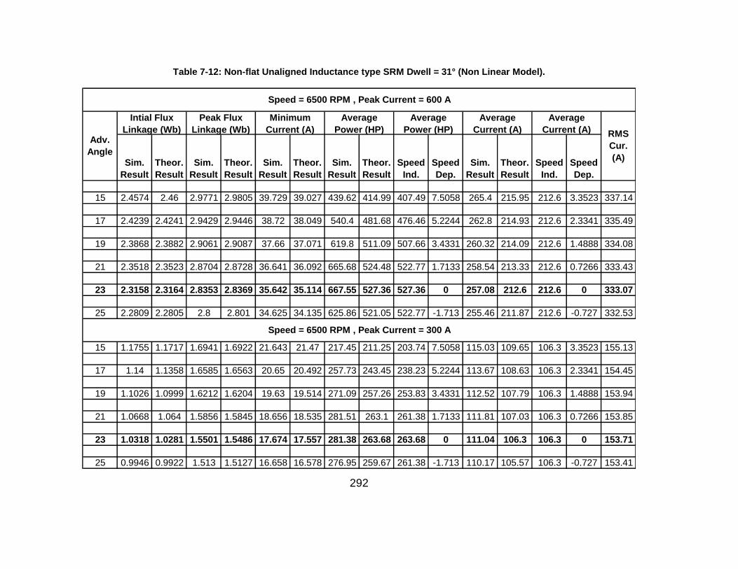
292

Table 7-12: Non-flat Unaligned Inductance type SRM Dwell = 31° (Non Linear Model).

Sim.

Result

Theor.

Result

Sim.

Result

Theor.

Result

Sim.

Result

Theor.

Result

Sim.

Result

Theor.

Result

Speed

Ind.

Speed

Dep.

Sim.

Result

Theor.

Result

Speed

Ind.

Speed

Dep.

15 2.4574 2.46 2.9771 2.9805 39.729 39.027 439.62 414.99 407.49 7.5058 265.4 215.95 212.6 3.3523 337.14

17 2.4239 2.4241 2.9429 2.9446 38.72 38.049 540.4 481.68 476.46 5.2244 262.8 214.93 212.6 2.3341 335.49

19 2.3868 2.3882 2.9061 2.9087 37.66 37.071 619.8 511.09 507.66 3.4331 260.32 214.09 212.6 1.4888 334.08

21 2.3518 2.3523 2.8704 2.8728 36.641 36.092 665.68 524.48 522.77 1.7133 258.54 213.33 212.6 0.7266 333.43

23 2.3158 2.3164 2.8353 2.8369 35.642 35.114 667.55 527.36 527.36 0 257.08 212.6 212.6 0 333.07

25 2.2809 2.2805 2.8 2.801 34.625 34.135 625.86 521.05 522.77 -1.713 255.46 211.87 212.6 -0.727 332.53

15 1.1755 1.1717 1.6941 1.6922 21.643 21.47 217.45 211.25 203.74 7.5058 115.03 109.65 106.3 3.3523 155.13

17 1.14 1.1358 1.6585 1.6563 20.65 20.492 257.73 243.45 238.23 5.2244 113.67 108.63 106.3 2.3341 154.45

19 1.1026 1.0999 1.6212 1.6204 19.63 19.514 271.09 257.26 253.83 3.4331 112.52 107.79 106.3 1.4888 153.94

21 1.0668 1.064 1.5856 1.5845 18.656 18.535 281.51 263.1 261.38 1.7133 111.81 107.03 106.3 0.7266 153.85

23 1.0318 1.0281 1.5501 1.5486 17.674 17.557 281.38 263.68 263.68 0 111.04 106.3 106.3 0 153.71

25 0.9946 0.9922 1.513 1.5127 16.658 16.578 276.95 259.67 261.38 -1.713 110.17 105.57 106.3 -0.727 153.41

Speed = 6500 RPM , Peak Current = 300 A

Intial Flux

Linkage (Wb)Adv.

Angle

Peak Flux

Linkage (Wb)

Minimum

Current (A)

Average

Power (HP) RMS

Cur.

(A)

Average

Current (A)

Average

Power (HP)

Average

Current (A)

Speed = 6500 RPM , Peak Current = 600 A

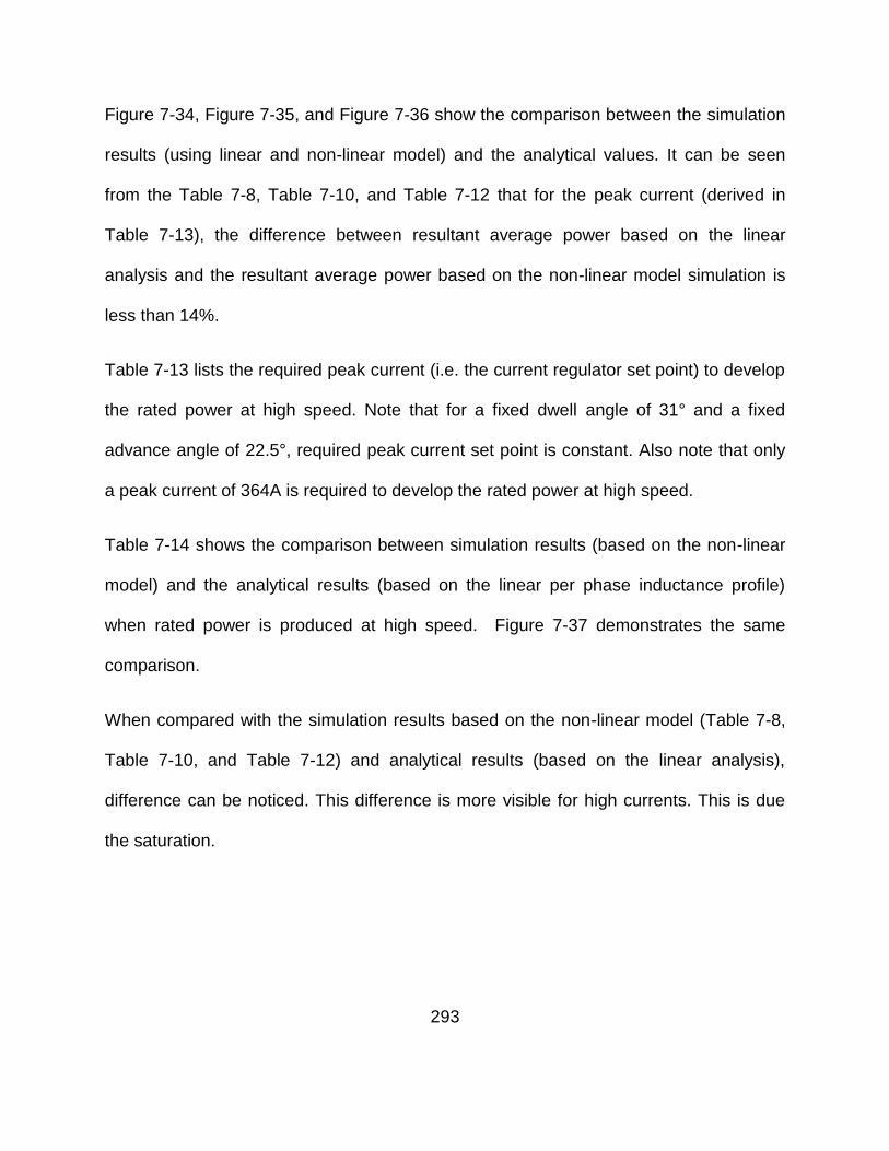
293

Figure 7-34, Figure 7-35, and Figure 7-36 show the comparison between the simulation

results (using linear and non-linear model) and the analytical values. It can be seen

from the Table 7-8, Table 7-10, and Table 7-12 that for the peak current (derived in

Table 7-13), the difference between resultant average power based on the linear

analysis and the resultant average power based on the non-linear model simulation is

less than 14%.

Table 7-13 lists the required peak current (i.e. the current regulator set point) to develop

the rated power at high speed. Note that for a fixed dwell angle of 31° and a fixed

advance angle of 22.5°, required peak current set point is constant. Also note that only

a peak current of 364A is required to develop the rated power at high speed.

Table 7-14 shows the comparison between simulation results (based on the non-linear

model) and the analytical results (based on the linear per phase inductance profile)

when rated power is produced at high speed. Figure 7-37 demonstrates the same

comparison.

When compared with the simulation results based on the non-linear model (Table 7-8,

Table 7-10, and Table 7-12) and analytical results (based on the linear analysis),

difference can be noticed. This difference is more visible for high currents. This is due

the saturation.

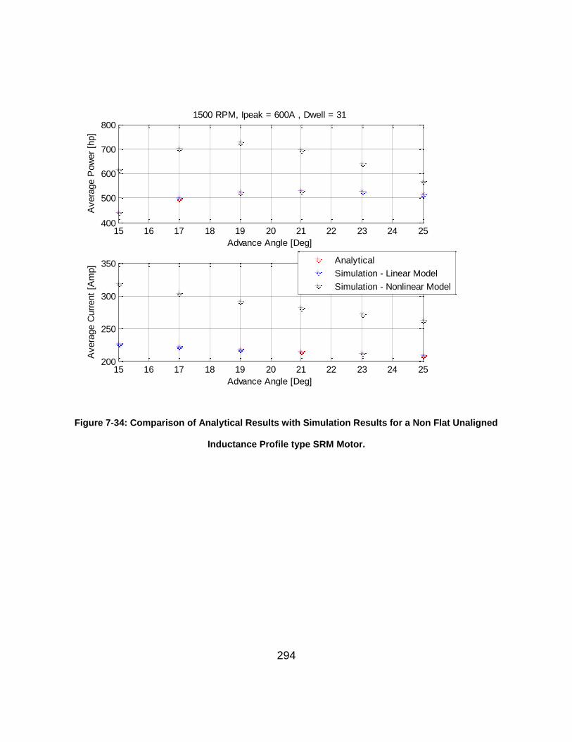
294

Figure 7-34: Comparison of Analytical Results with Simulation Results for a Non Flat Unaligned

Inductance Profile type SRM Motor.

15 16 17 18 19 20 21 22 23 24 25400

500

600

700

800

Advance Angle [Deg]

Avera

ge P

ow

er

[hp]

1500 RPM, Ipeak = 600A , Dwell = 31

15 16 17 18 19 20 21 22 23 24 25200

250

300

350

Advance Angle [Deg]

Avera

ge C

urr

ent

[Am

p]

Analytical

Simulation - Linear Model

Simulation - Nonlinear Model

295

Figure 7-35 : Comparison of Analytical and Simulation Results.

15 16 17 18 19 20 21 22 23 24 25400

500

600

700

Advance Angle [Deg]

Avera

ge P

ow

er

[hp]

3750 RPM, Ipeak = 600A , Dwell = 31

15 16 17 18 19 20 21 22 23 24 25200

220

240

260

280

Advance Angle [Deg]

Avera

ge C

urr

ent

[Am

p]

Analytical

Simulation - Linear Model

Simulation - Nonlinear Model

15 16 17 18 19 20 21 22 23 24 25200

250

300

Advance Angle [Deg]

Avera

ge P

ow

er

[hp]

3750 RPM, Ipeak = 300A , Dwell = 31

15 16 17 18 19 20 21 22 23 24 25100

105

110

115

120

Advance Angle [Deg]

Avera

ge C

urr

ent

[Am

p]

Analytical

Simulation - Linear Model

Simulation - Nonlinear Model

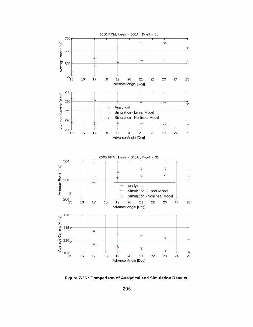
296

Figure 7-36 : Comparison of Analytical and Simulation Results.

15 16 17 18 19 20 21 22 23 24 25400

500

600

700

Advance Angle [Deg]

Avera

ge P

ow

er

[hp]

6500 RPM, Ipeak = 600A , Dwell = 31

15 16 17 18 19 20 21 22 23 24 25200

220

240

260

280

Advance Angle [Deg]

Avera

ge C

urr

ent

[Am

p]

Analytical

Simulation - Linear Model

Simulation - Nonlinear Model

15 16 17 18 19 20 21 22 23 24 25200

250

300

Advance Angle [Deg]

Avera

ge P

ow

er

[hp]

6500 RPM, Ipeak = 300A , Dwell = 31

15 16 17 18 19 20 21 22 23 24 25105

110

115

120

Advance Angle [Deg]

Avera

ge C

urr

ent

[Am

p]

Analytical

Simulation - Linear Model

Simulation - Nonlinear Model

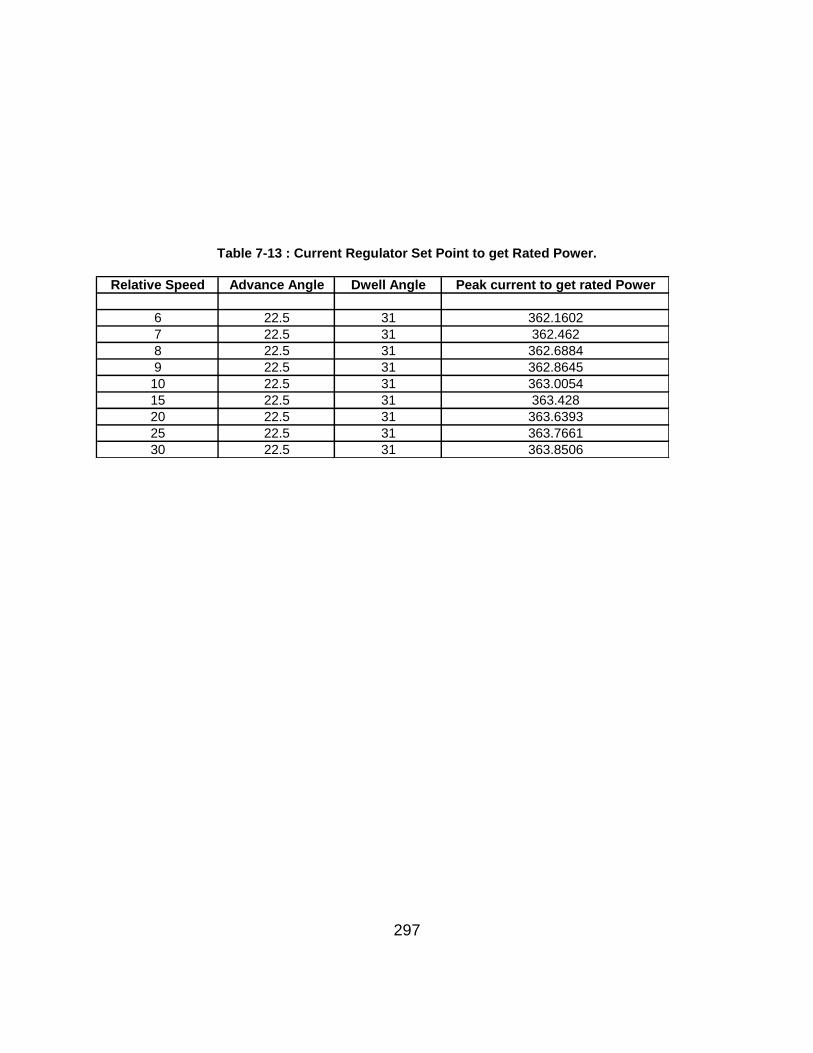
297

Table 7-13 : Current Regulator Set Point to get Rated Power.

Relative Speed Advance Angle Dwell Angle Peak current to get rated Power

6 22.5 31 362.1602

7 22.5 31 362.462

8 22.5 31 362.6884

9 22.5 31 362.8645

10 22.5 31 363.0054

15 22.5 31 363.428

20 22.5 31 363.6393

25 22.5 31 363.7661

30 22.5 31 363.8506

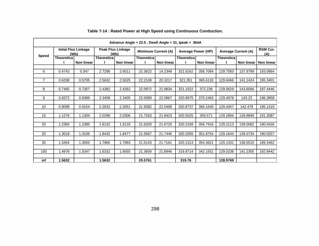
298

Table 7-14 : Rated Power at High Speed using Continuous Conduction.

Theoretica

l Non linear

Theoretica

l Non linear

Theoretica

l Non linear

Theoretica

l Non linear

Theoretica

l Non linear Non linear

6 0.4743 0.347 2.7298 2.6011 22.3622 14.2348 321.6162 356.7084 129.7583 137.9789 193.0864

7 0.6298 0.5705 2.5632 2.5025 22.2108 20.3217 321.351 365.6133 129.6466 141.1424 195.3401

8 0.7465 0.7357 2.4382 2.4262 22.0972 21.9834 321.1522 372.238 129.5629 143.6566 197.4446

9 0.8372 0.8389 2.3409 2.3405 22.0089 22.0867 320.9975 370.2463 129.4978 143.23 196.3858

10 0.9098 0.9154 2.2632 2.2651 21.9382 22.0498 320.8737 366.1549 129.4457 142.478 195.1419

15 1.1276 1.1304 2.0298 2.0306 21.7263 21.8423 320.5025 359.571 129.2894 139.8899 191.3087

20 1.2365 1.2385 1.9132 1.9133 21.6203 21.6725 320.3169 356.7916 129.2113 139.0082 190.0426

25 1.3018 1.3106 1.8432 1.8477 21.5567 21.7446 320.2055 351.8754 129.1644 139.0734 190.0257

30 1.3454 1.3505 1.7965 1.7993 21.5143 21.7161 320.1313 354.3621 129.1331 138.5515 189.3462

100 1.4978 1.5347 1.6332 1.6655 21.3659 21.8946 319.8714 342.1551 129.0238 141.2355 192.8442

inf 1.5632 1.5632 20.5761 319.76 128.9769

Advance Angle = 22.5 , Dwell Angle = 31, Ipeak = 364A

Average Current (A)Intial Flux Linkage

(Wb)Speed

Peak Flux Linkage

(Wb)Minimum Current (A) Average Power (HP)

RSM Cur.

(A)

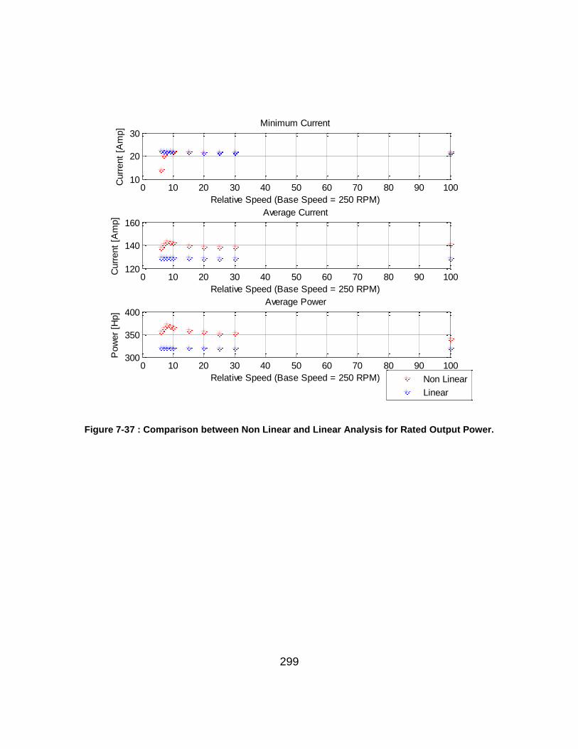
299

Figure 7-37 : Comparison between Non Linear and Linear Analysis for Rated Output Power.

0 10 20 30 40 50 60 70 80 90 10010

20

30

Relative Speed (Base Speed = 250 RPM)

Curr

ent

[Am

p]

Minimum Current

Non Linear

Linear

0 10 20 30 40 50 60 70 80 90 100120

140

160

Relative Speed (Base Speed = 250 RPM)

Curr

ent

[Am

p]

Average Current

0 10 20 30 40 50 60 70 80 90 100300

350

400

Relative Speed (Base Speed = 250 RPM)

Pow

er

[Hp]

Average Power

300

7.5.11 Controller Analysis

Figure 7-38 displays the RMS current and the developed power versus the advance

angle for dwell angles of 30.5o, 31.5o and 32.5o. The current regulator set point is fixed

at the 500A. Note that for a dwell of 32.5o, more RMS current is required for any

advance angle and less power is developed than a dwell angle of 31.5o. Same is true

when a dwell of 31.5° is compared to a dwell of 30.5°. This indicates that the greatest

efficiency can be achieved using a dwell that sufficient enough to sustain continuous

conduction, but otherwise as small as possible. There is an obvious need to precisely

determine the dwell as the motor may slip from continuous to discontinuous conduction

with precipitous loss of the developed power if the dwell angle is reduces below 30°.

Also, note that the RMS current is independent of the advance angle and depends only

on the dwell angle.

While the developed power varies with the advance angle, adjustment of the advance

angle is not the best way to control the developed power. The best method for power

control is the current regulator set point. As shown in the Figure 7-39, output power can

be efficiently controlled by changing the current regulator set point rather than changing

the advance angle or the dwell angle.

Dynamic response to an increased power command can be very sluggish if the

minimum dwell is used. Figure 7-40 shows the simulated response of the motor current

to a step change in the current regulator set point from an initial value of 0A to 364A

when operating at relative speed of 13. Simulations were carried out for a dwell of 30.5o

and for a dwell of 33.5o.

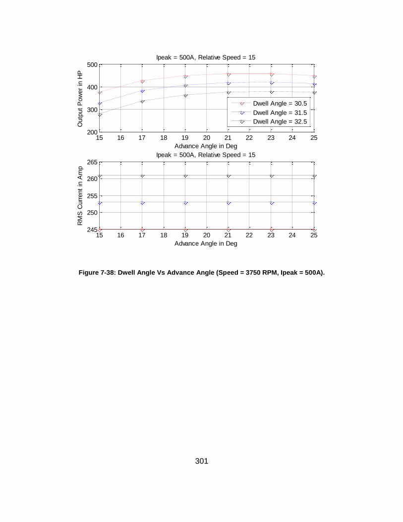
301

Figure 7-38: Dwell Angle Vs Advance Angle (Speed = 3750 RPM, Ipeak = 500A).

15 16 17 18 19 20 21 22 23 24 25200

300

400

500

Advance Angle in Deg

Outp

ut

Pow

er

in H

P

Ipeak = 500A, Relative Speed = 15

Dwell Angle = 30.5

Dwell Angle = 31.5

Dwell Angle = 32.5

15 16 17 18 19 20 21 22 23 24 25245

250

255

260

265

Advance Angle in Deg

RM

S C

urr

ent

in A

mp

Ipeak = 500A, Relative Speed = 15

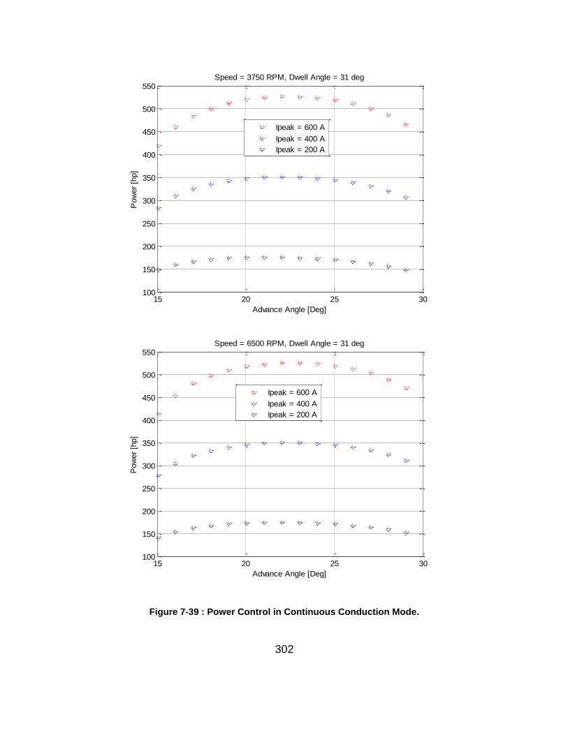
302

Figure 7-39 : Power Control in Continuous Conduction Mode.

15 20 25 30100

150

200

250

300

350

400

450

500

550

Advance Angle [Deg]

Pow

er

[hp]

Speed = 3750 RPM, Dwell Angle = 31 deg

Ipeak = 600 A

Ipeak = 400 A

Ipeak = 200 A

15 20 25 30100

150

200

250

300

350

400

450

500

550

Advance Angle [Deg]

Pow

er

[hp]

Speed = 6500 RPM, Dwell Angle = 31 deg

Ipeak = 600 A

Ipeak = 400 A

Ipeak = 200 A

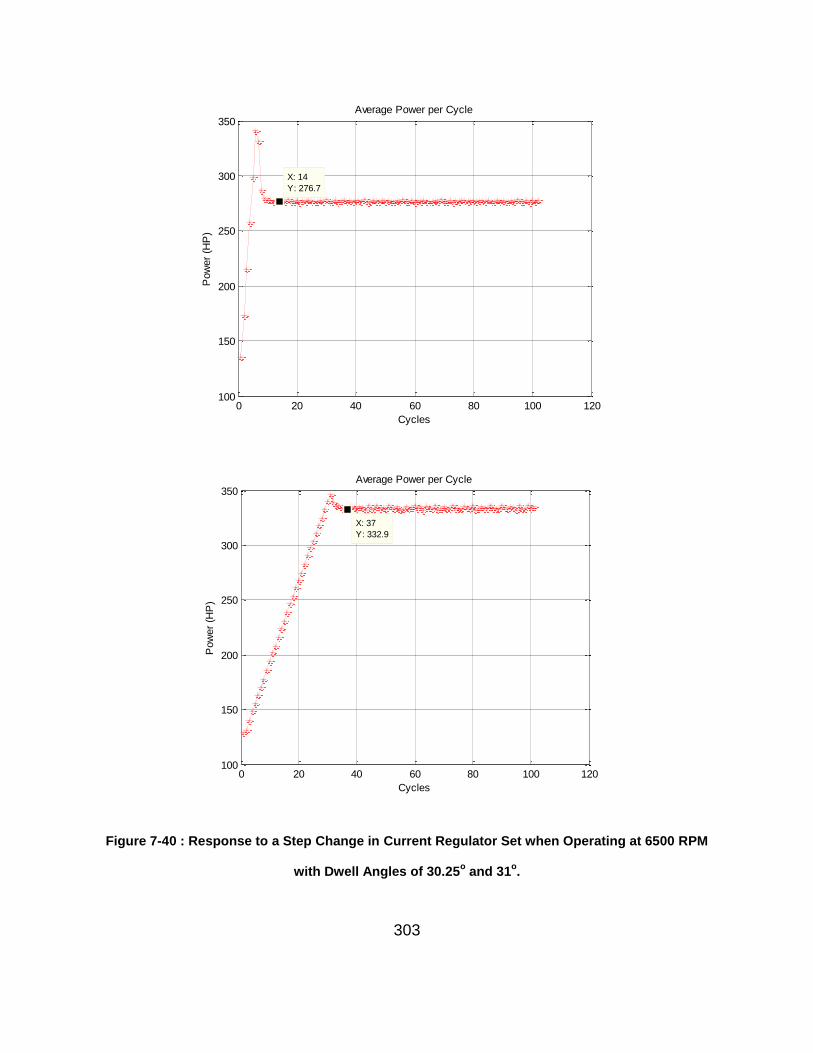
303

Figure 7-40 : Response to a Step Change in Current Regulator Set when Operating at 6500 RPM

with Dwell Angles of 30.25o and 31

o.

0 20 40 60 80 100 120100

150

200

250

300

350

X: 14

Y: 276.7

Cycles

Pow

er

(HP

)

Average Power per Cycle

0 20 40 60 80 100 120100

150

200

250

300

350

X: 37

Y: 332.9

Cycles

Pow

er

(HP

)

Average Power per Cycle

304

In both cases, the advance angle is 22.5o. Observe that for a dwell of 30.5o,

approximately 37 cycles are required to achieve 364A but developed power is about

333Hp; while for a dwell of 33.5o, only 14 cycles are required but the output power is

276Hp. Smaller dwell yields greater steady state efficiency but it has considerably

longer dynamic response time. Application requirements may dictate how to deal with a

tradeoff between the speed of response and the steady state efficiency. If both are

desired, a smart controller can be developed using the analytical formulas, derived in

previous section. Based on the power requirement, current regulator set point can be

estimated by using Equation (7.99). Initially the dwell angle can be set to the maximum

possible value to get faster response. Bases the dwell angle, power maximizing

advance angle can be selected by using Equation (7.97). Based on this information it is

possible to estimate the number of strokes it will take to achieve the steady state by

using Equation (7.98). As the motor current approaches the current regulator set point,

the dwell angle can be collapsed back to the minimum possible value (at least 50% of

the stroke length). With the dwell, advance angle also can be changed in small

increments.

7.5.12 Constant Power Speed Ratio

Linear analysis similar to the one in Section 7.4.10 can be carried out to find out the

resultant output power for a non flat type SRM motor when operated in single pulse

mode at speed with discontinuous type conduction. This analysis is based on the linear

inductance waveform. Figure 7-41 illustrates the same. Some saturation can be

observed for medium speeds, especially with the high current.

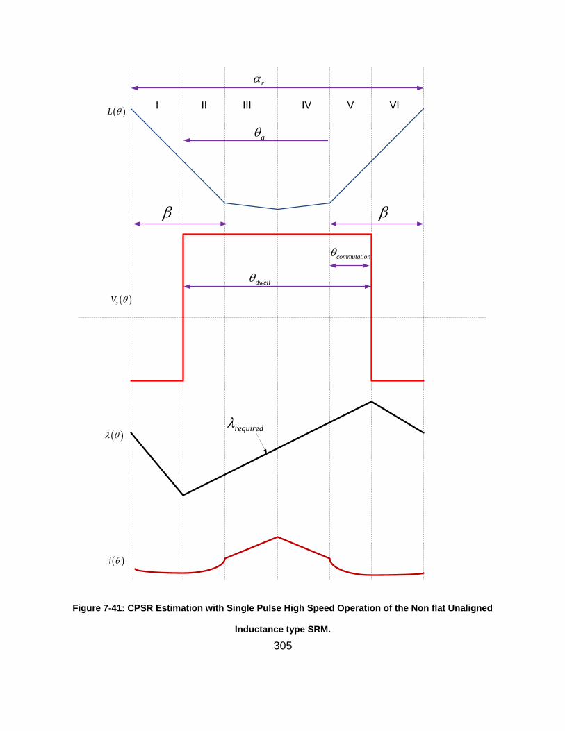
305

required

I II III IV V VI

r

a

commutation

dwell

L

sV

i

Figure 7-41: CPSR Estimation with Single Pulse High Speed Operation of the Non flat Unaligned

Inductance type SRM.

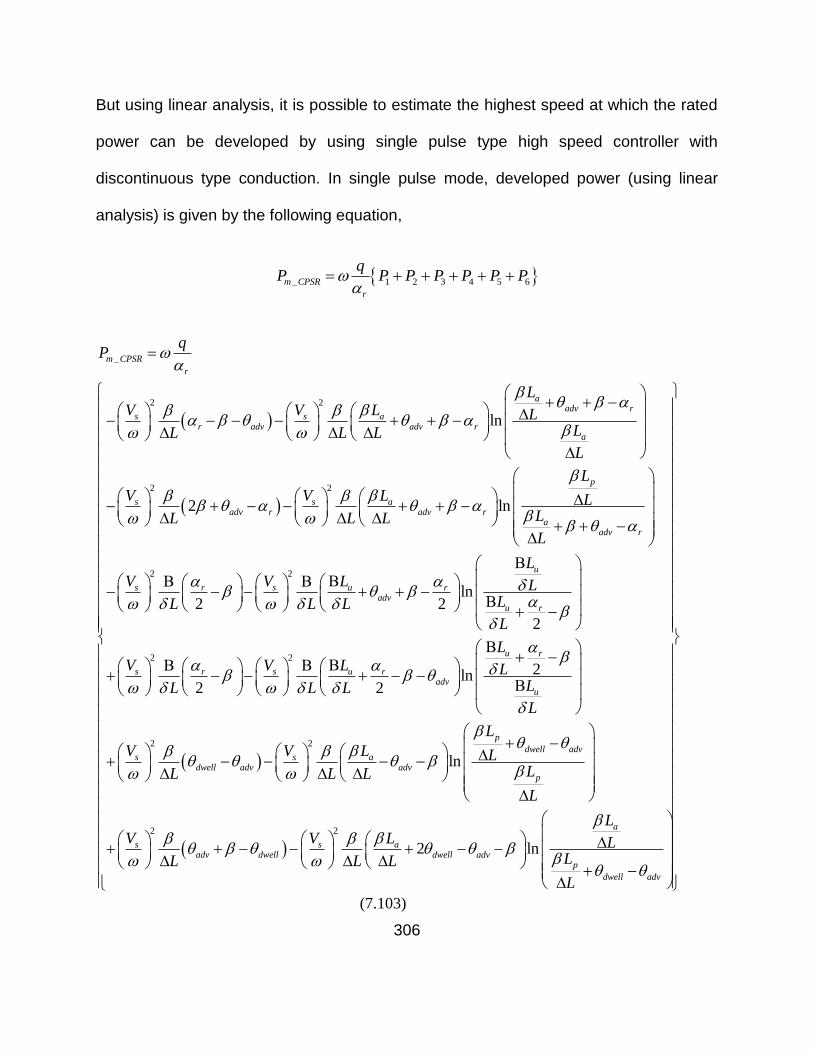
306

But using linear analysis, it is possible to estimate the highest speed at which the rated

power can be developed by using single pulse type high speed controller with

discontinuous type conduction. In single pulse mode, developed power (using linear

analysis) is given by the following equation,

_ 1 2 3 4 5 6m CPSR

r

qP P P P P P P

_

2 2

2 2

ln

2 ln

m CPSR

r

aadv r

s s ar adv adv r

a

p

s s aadv r adv r

aadv r

s

qP

LV V L L

LL L L

L

L

V V L LLL L L

L

V

2 2

2 2

2

ln2 2

2

2ln2 2

u

s ur radv

u r

u r

s s ur radv

u

sdwell adv

LV L L

LL L L

L

LV V L L

LL L L

L

V V

L

2

2 2

ln

2 ln

p

dwell advs a

advp

a

s s aadv dwell dwell adv

p

dwell adv

L

L LLL L

L

LV V L L

LL L L

L

(7.103)

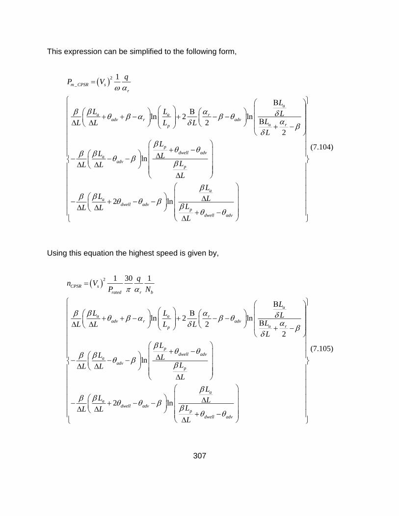
307

This expression can be simplified to the following form,

2

_

1

ln 2 ln2

2

ln

2 ln

m CPSR s

r

u

a a radv r adv

u rp

p

dwell adva

advp

a

adwell adv

qP V

LL L L

LL L L L

L

L

L LLL L

L

LL L

LL L

p

dwell advL

(7.104)

Using this equation the highest speed is given by,

2 1 30 1

ln 2 ln2

2

ln

2

CPSR s

rated r b

u

a a radv r adv

u rp

p

dwell adva

advp

adwell adv

qn V

P N

LL L L

LL L L L

L

L

L LLL L

L

L

L L

ln

a

p

dwell adv

L

LL

L

(7.105)

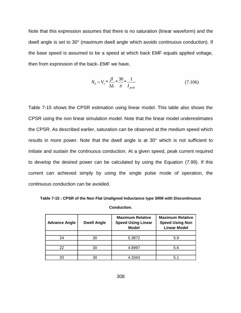
308

Note that this expression assumes that there is no saturation (linear waveform) and the

dwell angle is set to 30° (maximum dwell angle which avoids continuous conduction). If

the base speed is assumed to be a speed at which back EMF equals applied voltage,

then from expression of the back-.EMF we have,

30 1

* * *b s

peak

N VL I

(7.106)

Table 7-15 shows the CPSR estimation using linear model. This table also shows the

CPSR using the non linear simulation model. Note that the linear model underestimates

the CPSR. As described earlier, saturation can be observed at the medium speed which

results in more power. Note that the dwell angle is at 30° which is not sufficient to

initiate and sustain the continuous conduction. At a given speed, peak current required

to develop the desired power can be calculated by using the Equation (7.99). If this

current can achieved simply by using the single pulse mode of operation, the

continuous conduction can be avoided.

Table 7-15 : CPSR of the Non Flat Unaligned Inductance type SRM with Discontinuous

Conduction.

Advance Angle Dwell Angle

Maximum Relative

Speed Using Linear

Model

Maximum Relative

Speed Using Non

Linear Model

24 30 5.3872 5.9

22 30 4.8997 5.6

20 30 4.3343 5.1

309

8 CONCLUSION AND FUTURE WORK

8.1 Surface Permanent Magnet Synchronous Motor

Experimental results confirm that the conventional phase advancement method based

high-speed controller can produce the rated power without exceeding the current limit;

provided the surface PM motor has “sufficient” per phase winding inductance. This

controller is based on three simple equations. In the constant torque region, required

motor current can be estimated based on the torque requirement. Based on this current

requirement, required voltage magnitude and phase angle can be estimated by solving

a fundamental frequency model. Using this voltage magnitude, PWM modulation index

can then be calculated. In this region, the supply voltage magnitude and phase angle is

adjusted such that the resultant motor current is in phase with the back-EMF. This

produces maximum torque-per-amp. Similarly, in the constant power region, it is

possible to estimate the required motor current based on the power requirement. Based

on this current requirement, required voltage phase angle can be calculated by solving

a fundamental frequency model. Note that in this region, the applied voltage is a square

wave and the voltage magnitude is at the rated value. In this region, the only thing that

can be changed is the voltage phase angle. Hence, this method is called the phase

advancement method.

The CPA method is mathematically much simpler when compared to the traditional

vector control based field weakening schemes. This CPA method does not require

310

phase current or phase voltage measurements or any three-phase to two-phase

transformations. This reduces the controller/hardware size and cost, and also increases

the reliability of the controller. When using the CPA method, in the field-weakening

region, the motor current decreases to a minimum value. At this speed, which is

referred to as the “minimum speed”, the power factor is at unity. Also at this speed, the

inverter operates in the over-modulation region. Therefore, the inverter efficiency is at

its best. The magnitude of this resultant minimum current depends inversely on the

maximum possible inverter output voltage. Since can be increased by raising the

DC supply voltage, a further reduction in the motor current and inverter losses can be

achieved. If the traction drive spends a significant amount of time at a certain speed,

machine/control parameters can be adjusted so that this minimum speed is the same as

the nominal speed of that motor. Above this minimum speed, current slowly increases to

a constant value called as “characteristic current”. In theory, if this current is less than

the rated current of the motor, the CPSR can be infinite when a proper control method is

used. The use of fractional-slot concentrated windings increases the per phase

inductance, which in turn reduces this characteristic current of the surface PM motors

below the rated current.

With the constant voltage, constant power method (described in Section 2.1.1), above

base speed, the stator current decreases continuously. With the constant current,

constant power vector control method (described in Section 2.1.2), the stator current

remains constant throughout the constant power region. In the optimum current vector

control method (described in Section 2.1.3), the stator current remains constant till the

maxV

311

current-limit circle intersects the voltage-limit circle when the motor is above speed.

After this point the stator current decreases because the d-axis component remains

constant while the q-axis component decreases continuously.

During experimentation, it was possible to use a step size of 50 μs and 9 kHz PWM

switching frequency was implemented. As the PWM switching was implemented in the

software itself, it is also possible to implement the PWM control in the hardware. This

will further increase accuracy and reliability and will further reduce computational

requirement. Since the CPA method does not work directly with the torque producing

component of the phase current, it is not as accurate as the vector control method. At

high speed, since the phase current approaches a constant value, partial load efficiency

of surface PM motors is not as good as full load efficiency. Since the CPA method does

not work directly with field weakening component of the stator current, it is difficult to

comment on the possibility of rotor demagnetization. Following is a list of future work

recommendations.

1. Compare the CPA method results with vector control schemes in terms of id-iq

components and various efficiencies, especially partial load efficiency.

2. Modify the CPA method to improve partial load efficiency.

3. Modify the CPA method to allow regenerative breaking.

4. Sinusoidal PWM was implemented inside the OPAL RT software. A significant

portion of computational power was used to carry out sine-triangle comparison

and produce switching pattern. During experimentation, it was observed that

switching becomes unstable around the modulation index of 1. Implementing

312

SPWM in the hardware (FPGA) will not only free up a lot of computational power,

it will also increase accuracy, stability and reliability. This might also improve

inverter and motor efficiency.

5. Sufficient measurements need to be carried out at different DC voltages to see

the effect of a supply voltage increase on motor and inverter efficiency.

6. Study the effect of the CPA method on rotor demagnetization.

8.2 Switched Reluctance Motor

Analytical and simulation results suggest that the continuous conduction can be used to

develop the rated power at high speed. Analysis of the linear magnetic model has

resulted in analytical expressions relating average motor power and current to the

machine and control parameters. It also resulted in analytical expressions for the

residual flux linkage and peak current required to produce this desired output power.

Analytical and simulation results suggest that the peak current required to develop this

rated power as well as the resultant average and RMS current are well below the rated

values. Analytical equations suggest that the resultant average power and current can

be split into a speed dependent and independent part. The dependent part of both the

average power and current approaches to zero as the speed increases.

Analytical and simulation results also suggest that it is possible to sustain the

continuous conduction by using a current regulator. Analytical results (no. of strokes

required to achieve steady state) suggest that by maintaining the dwell angle at more

313

than 50% of the stroke length, it is possible to initiate the continuous conduction. Since

the fluxing region is more than the de-fluxing region, residual and peak flux-linkages

grow from cycle to cycle. With the flux-linkages, phase current also grows from cycle to

cycle. Once the desired peak current is reached, the current regulator imposes a zero

volt-sec interval such that the resultant width of the fluxing region will be same as the

de-fluxing region.

The speed independent part of the average power depends on the dwell angle, advance

angle, peak current and the machine design parameters, while the speed independent

part of the average current only depends on the peak current and machine design

parameters. Hence, the current regulator set-point is the best way to regulate the output

power rather than the advance or dwell angle. This results in the motor current being

proportional to the output power.

It has been shown that the minimum dwell necessary to initiate and sustain continuous

conduction, provides the maximum watts per amp control and results in minimum

average current. However, it results in a slow response. The time required to achieve

the steady state decreases exponentially with the increase in the dwell angle. Therefore

it is possible to compromise between the speed of the response and the output

efficiency.

Analytical and simulation results suggest that, for a non-flat type SRM there is a well

defined combination of the advance and dwell angle which reduces the speed

dependent part of both the average power and current to zero. Naturally, this

314

combination results into maximum efficiency as the resultant average power and current

is nothing but the speed independent part. This combination (that satisfies Equation

(7.97)) does not depend on the speed. Therefore, in this type of SRM motor, the dwell

and the advance angle can be kept constant to this combination, and the resultant peak

current required to produce the rated power will also remain constant for the entire high

speed range. Simulation results also suggest that for both types of SRM motors, the

resultant RMS current remains constant for a fixed dwell angle.

It has been shown that high speed continuous conduction control has the same control

variables as low-speed discontinuous conduction. Based on speed information and

power requirement, desired peak current can be estimated by using the Equation (7.47)

/(7.99) . If this peak current is less than the current estimated by Equation (7.54), the

traditional discontinuous conduction type control scheme can be used to develop the

desired output power. Otherwise, continuous conduction can be initiated and sustained

by keeping the dwell angle constant (more than 50% of the stroke length). Based on this

dwell angle, proper advance angle, which maximizes output power, can be selected by

using Equation (7.48)/(7.97). By using Equation (7.53)/(7.98), it is also possible to

estimate the number of strokes it will take to achieve steady state.

From analytical and simulation results, it can be seen that in continuous conduction with

the current levels required to produce rated power, magnetic saturation is not a

significant factor.

Following is a list of recommended future work.

315

1. Literature [13],[75] suggests that continuous conduction does not offer any

benefits at low speed or the higher speed at which rated power can be developed

using the traditional discontinuous type conduction. A smart controller, which can

co-ordinate between the low and medium speed discontinuous conduction, and

high speed continuous conduction needs to be developed.

2. References [76] and [16] describe a list of the machine parameters that affect the

highest speed at which the rated power can be developed by using the

discontinuous type single pulse operation. Similar analysis needs to be done on

machine parameters that affect continuous conduction.

3. Figure 7-18 shows the effect of saturation on per phase inductance profile.

Instead of using a linear inductance profile (straight lines), use of upward

parabola to represent the per phase inductance profile might result in more

accurate analytical expressions describing the behavior of switched reluctance

motors when operated in continuous conduction.

4. Minimum dwell yields the maximum power but the slowest response. High dwell

can result in faster response but low output power. If both are desired, initially the

dwell angle can be kept as large as possible, and as the peak current is

approached, this dwell angle can be collapsed back to the minimum possible

value. This needs to be confirmed.

316

Bibliography

317

Bibliography

[1] W. L. Soong and T. J. E. Miller, "Field Weakening Performance of Brushless

Synchronous AC Motor Drives," IEE Proceedings of the Electronic Power

Application, vol. 141, no. 6, pp. 331 - 340, November 1994.

[2] L. H. Ward, "Volts Vs Ohms - The Speed Regulation of Electric Motors," AIEE

Transactions, vol. 13, pp. 375 - 384, 1896.

[3] P. L. Alger and R. E. Arnodl, "The History of Induction Motors in America,"

Proceedings of IEEE, pp. 1380 - 1383, September 1976.

[4] T. J. E. Miller, Switched Reluctance Motors. Oxford: Magna Physics Publishing and

Clarendon Press, 1993.

[5] P. Pillay and R. Krishnan, "Modeling, Simulation and Analysis of Permanent

Magnet Motor Drives : Part I - The Permanent Magnet Synchronous Motor Drive,"

IEEE Transactions on Industry Applications, vol. 25, no. 2, pp. 265-273, March/April

1989.

[6] P. Pillay and R. Krishnan, "Modeling, Simulation and Analysis of Permanent

Magnet Motor Drives : Part II - The Brushless DC Motor Drive," IEEE Transactions

on Industry Applications, vol. 25, no. 2, pp. 274 - 279, March / April 1989.

[7] N. A. Patil, J. S. Lawler, and J. W. McKeever, "Determining constant power speed

318

ratio of the induction motor from equivalent circuit parameters," IEEE Southeastcon,

pp. 460 - 467 , April 2008.

[8] T. M. Jahns, "Flux Weakening Regime Operation of an Interior Permanent Magnet

Synchronous Motor Drive," IEEE Transaction on Industry Application, vol. 23, pp.

681 - 689, July / August 1987.

[9] S. Morimoto, Y. Takeda, T. Hirasa, and K. Taniguchi, "Expansion of Operating

Limits for Permanent Magnet Motor by Current Vector Control Considering Inverter

Capacity," IEEE Transactions on Industrial Application, vol. 26, pp. 866 - 871, 1990.

[10] Cambier, "Brushless DC Motor Using Phase Timing Advancement.," 5,677,605,

Octomber 14, 1997.

[11] S. R. MacMinn and J. W. Sember, "Control of a Switched-Reluctance Aircraft

Engine Starter-Generator Over a Very Wide Speed Range," Proceedins of Energy

Conversion Engineering Conference, IECEC-89, pp. 631 - 638, August 1989.

[12] S. R. MacMinn and W. D. Jones, "A Very High Speed Switched-Reluctance Starter-

Generator for Aircraft Engine Application," Proceedings of IEEE National

Aerospace and Electronics Conference, NAECON, vol. 4, pp. 1758 - 1764, May

1989.

[13] J. S. Lawler, J. M. Baily, J. W. McKeever, and P. J. Otaduy, "Impact of Continuous

Conduction on the Constant Power Speed Range of the Switched Reluctance

319

Motor," IEEE International Conference on Electrical Machines and Drives, pp. 1285

- 1292, May 2005.

[14] R. Krishnan, Switched Reluctance Motor Drives : Modeling, Simulation, Analysis,

Design, and Applications.: CRC Press, 2001.

[15] T. J. E. Miller, Switched Reluctance Motors and their Control.: Magna Physics

Publications , Oxford University Press, 1993.

[16] M. Rekik et al., "High-Speed-Range Enhancement of Switched Reluctance Motor

with Continuous Mode for Automotive Applications," European Transactions on

Electrical Power, 2007.

[17] T. Sebastian and G. R. Slemon, "Operating Limits of Inverter-Driven Permanent

Magnet Motor Drives," IEEE Transaction on Industry Application, vol. IA-23, no. No.

2, pp. 327 - 333, March/April 1987.

[18] E. Clarke, Circuit Analysis of A-C Power Systems Vol. 1 - Symmetrical and Related

Components. New York, U.S.: John Willey and Sons, 1943.

[19] B. K. Bose, Power Electronics and AC Drives. New Jersey, U.S.: Prentice - Hall,

1986.

[20] P. C. Kraus, Analysis of Electrical Machinery.: McGraw - Hill, Inc., 1986.

[21] R. H. Park, "Two - Reaction Theory of Synchronous Machines - Generalized

320

Method of Analysis - Part - I," AIEE Transaction , vol. 48, pp. 716 - 727, July 1929.

[22] P. Vas, Sensorless Vector and Direct Torque Control.: Oxford University Press,

1999.

[23] J. S. Lai, J. M. Baily, R. W. Young, C. W. Johns, and R. A. Hawsey, "Optimum

Current for a High-Speed Axial Air Gap Permanent Magnet Synchronous Motor,"

IEEE - IAS Annual Meeting, vol. Conference Records, pp. 767 - 772, 1989.

[24] J. M. Baily, J. S. Lawler, and H. W. Blake, "Field-Weakening Schemes and Magnet-

Retention Techniques for Permanent Magnet Machines," Oak Ridge National Lab.,

Unpublished ORNL-TM 74, 1999.

[25] D. W. Novotny and T. A. Lipo, Vector Control and Dynamics of AC Drives. New

York, U.S.: Oxford University Press, Inc., 1996.

[26] F. Magnussen, P. Thelin, and C. Sadarangani, "Performance Evaluation of

Permanent Magnet Synchronous Machines with Concentrated and Distributed

Windings Including Effect of Field Weakening," Proceedings of 2nd IEE

International Conference on Power Electronics, Machines and, Drives, vol. 2, pp.

679 - 685, March / April 2004.

[27] A. M. El-Refaie, T. M. Jahns, P. J. McCleer, and J. W. McKeever, "Experimental

Verification of Optimal Flux Weakening in Surface PM Machines Using

Concentrated Windings," IEEE Transaction on Industry Application , vol. 42, no. 2,

321

pp. 443 - 453, March / April 2006.

[28] S. Morimoto, Y. Takeda, and T. Hirasa, "Current Phase Control Methods for

Permanent Magnet Synchronous Motors," IEEE Transactions on Power Electronics

, vol. 5, no. 2, pp. 133 - 139, April 1990.

[29] S. Morimoto, T. Ueno, M. Sanada, and A. Yamagiwa, "Effects and Compensation of

Magnetic Saturation in Permanent Magnet Synchronous Motor Drives," IEEE

Transactions on Industry Application, vol. 30, no. 6, pp. 59 - 64, November /

December 1994.

[30] A. Kumamoto and Y. Hirane, "A Semi-Closed Loop Torque Control of a Buried

Permanent Magnet Motor Based on a New Flux-Weakening Approach," IEEE - IAS

Annual Meeting , vol. Conference Recordings, pp. 656 - 661, 1989.

[31] A. M. EL-Refaie, D. W. Novotny, and T. M. Jahns, "A Simple Model for Flux

Weakening in Surface PM Synchronous Machines Using Back-to-Back Thyristors,"

IEEE Power Electronics Letters, vol. 2, no. 2, pp. 54-57, June 2004.

[32] R. Monajemy and R. Krishnan, "Performance Comparison for Six-Step Voltage and

Constant Back EMF Control Stratergies for PMSM," IEEE Industry Applications

Conference , vol. 1, pp. 165 - 172, 1999.

[33] G. R. Slemon, "Achieving a Constant Power Speed Range for PM Drives," IEEE

Transactions on Industry Application, vol. 31, no. 2, pp. 368 - 372, March / April

322

1995.

[34] G. R. Slemon and X. Liu, "Modeling and Design Optimization of Permanent Magnet

Machines," Electrical Machines and Power System, vol. 20, pp. 71 - 92, 1992.

[35] P. L. Chapman and P. T. Krein, "Motor Re-Rating for Traction Application - Field

Weakening Revisited," Electrical Machines and Drives Conference, IEMDC, vol. 3,

pp. 1388 - 1391, June 2003.

[36] E. Nipp, "Alternative to Field - Weakening of Surface - Mounted Permanent -

Magnet Motors for Variable - Speed Drives," IEEE Industry Applications

Conference, vol. 1, pp. 191 - 198, Octomber 1995.

[37] J. S. Lawler, "Control of Surface Mounted Permanent Magnet Motors with Special

Application to Fractional - Slot Motors with Concentrated Windings," Oak Ridge

National Laboratory, Oak Ridge, Internal ORNL/TM-2005 / 184, 2005.

[38] T. D. Gillespie, Fundamentals of vehicle dynamics., 1992.

[39] A. M. EL-Refaie, T. M. Jahns, P. B. Reddy, and J. W. McKeever, "Modified Vector

Control Algorithm for Increasing Partial-Load Efficiency of Fractional-Slot

Concentrated-Winding Surface PM Machines," IEEE Transactions on Industry

Applications, vol. 44, no. 5, pp. 1543 - 1551, September / October 2008.

[40] P. B. Reddy and T. M. Jahns, "Impact of Winding Layer Number and Slot/Pole

Combination on AC Armature Losses of Synchronous Surface PM Machines

323

Designed for Wide Constant-Power Speed Range Operation," Industry Applications

Society Annual Meeting, pp. 1 - 8, October 2008.

[41] A. M. EL-Refaie, T. M. Jahns, P. B. Reddy, and J. W. Mckeever, "Modified Vector

control Algorithm for Increasing Partial-Load Efficiency of Fractional-Slot

Concentrated-Winding Surface PM Machines," IEEE Transaction on Industry

Applications, vol. 44, no. 5, pp. 1543 - 1551, September / October 2008.

[42] M. Chuntung, G. R. Slemon, and R. Bonnert, "Modeling of Iron Losses in Surface-

Mounted Permanent Machine Synchronous Motors," Industry Applications

Conference, vol. 4, pp. 2585 - 2591, 2001.

[43] K. Atallah, D. Howe, P. H. Mellor, and D. A. Stone, "Rotor Loss in Permanent

Magnet Brushless AC Machines," International Conference on Electrical Machines

and Drives , pp. 60 - 62, May 1999.

[44] P. H. Mellor, R. Wrobel, and N. McNeill, "Investigation of Proximity Losses for High

Speed Brushless Permanent Magnet Motor," Industry Application Conference, vol.

3, pp. 1514 - 1518.

[45] J. S. Lawler, J. M. Baily, and J. W. McKeever, "Minimum Current Magnitude Control

of Surface PM Synchronous Machines during Constant Power Operation," IEEE

Power Electronics Letters, vol. 3, no. 2, pp. 53 - 56, 2005.

[46] D. A. Staton, W. L. Soong, C. Cossar, and T. E. Miller, "Unified Theory of Torque

324

Production in Switched Reluctance and Synchronous Reluctance Motors,"

International Conference on Electrical Machines and Drives, pp. 67 - 72, September

1993.

[47] C. Elmas and H. Zelaya De La Parra, "A DSP Controlled Switched Reluctance

Drive System for Wide Range of Operating Speeds," Power Electronics Specialists

Conference, PESC, vol. 2, pp. 844 -850, June - July 1992.

[48] S. R. MacMinn and W. D. Jones, "A Very High Speed Switched-Reluctance Starter-

Generator for Aircraft Engine Application," Proceedings of IEEE National

Aerospace and Electronics Conference, NAECON, vol. 4, pp. 1758 - 1764, May

1989.

[49] C. E. Green, "Control of Switched Reluctance Machines," B1 6,351,094, February

26, 2002.

[50] R. C. Becerra, M. Ehsani, and T. E. Miller, "Commutation of SR Motors," IEEE

Transactions of Power Electronics, vol. 8, no. 3, pp. 257 - 263, July 1993.

[51] R. Krishnan, Switched Reluctance Motor Drives : Modeling, Simulation, Analysis,

Design and Applications.: CRC Press LLC, 2001.

[52] T. T. e. a. Borges, "Switched Reluctance Motor Drive at High Speeds, with Control

of Current," IEEE International Electrical Machines and Drives Conference

Records, pp. TB1/12.1 - TB1/12.3, May 1997.

325

[53] B. C. Mecrow, "Control of a Switched Reluctance Drive," 7205694, April 17, 2007.

[54] I. Jordison et al., "Control of a switched reluctance drive," 6972533, July 18, 2003.

[55] M. P. Tankard, "Control Strategy for a switched Reluctance Drive Systems,"

6759826, July 6, 2004.

[56] C. E. B. Green, "Control of Switched Reluctance Machines," 6291949, September

18, 2001.

[57] C. R. Elliott, "Hysteresis Current Controller for a Reluctance Machine," 5998945,

December 7, 1999.

[58] C. R. Elliott, "on-off controller," 5926011, July 20, 1999.

[59] J. J. Gribble, P. C. Kjaer, and T. J. E. Miller, "Optimal Commutation in Average

Torque Control of Switched Reluctance Motors," IEE Proceedings of Electric Power

Applications, vol. 146, no. 1, pp. 2 - 10, January 1999.

[60] I. Husain, Electric and Hybrid Electric Vehicles Design Fundamentals.: CRC Press.

[61] R. B. Inderka, M. Menne, and R. W. A. A. De Doncker, "Control of Switched

Reluctance Drives for Electrical Vehicle Applications," IEEE Transactions on

Industrial Electronics, vol. 49, no. 1, pp. 48 - 53, February 2002.

[62] P. C. Kjaer, C. Cossar, and T. J. E. Miller, "Very High Bandwith Digital Current

Controller for High-Performance Motor Drives," Proceedings of Power Electronics

326

and Variable-Speed Drives Conference, pp. 185 - 190, September 1996.

[63] B. G. Hexamer, "Implementing of Closed-Loop Controllers for Switched Reluctance

Drives on Microcontrollers and DSP Controllers," Proceedings of EPE, 1999.

[64] H. Bausch, A. Grief, B. Lange, and R. Bautz, "A 50 kW / 1500 RPM Switched

Reluctance Drive for an Electrical Vehicle : Current Control and Performance

Characteristics," Proceedings of International Conference on Electrical Machines,

pp. 603 - 607, August 2000.

[65] B. K. Bose, T. J. E. Miller, P. M. Szczesny, and W. H. Bicknell, "Microcomputer

Control of Switched Reluctance Motor," IEEE Transactions on Industry

Applications, vol. IA - 22, no. 4, pp. 708 - 715, July - August 1986.

[66] W. F. Ray, R. M. Davis, and R. J. Blake, "THe Control of SR Motors," Proceedings

of the Conference on Applied Motion Control, pp. 137 - 145, June 1986.

[67] B. Fahimi, Y. Gao, and M. Ehsani, "On Suitability of Switched Reluctance Motor

Drives for 42 Volts Super High Speed Operation: Application to Automotive Fuel

Cells ," The 27th Annual Conference of the IEEE Industrial Electronics Society, pp.

1947 - 1951, 2001.

[68] K. M. Rahman, B. Fahimi, G. Suresh, and M. Ehsani, "Advantages of Switched

Reluctance Motor Application to EV and HEV: Design and Control Issues," IEEE

Transactions on Industry Applications, vol. 36, no. 1, pp. 111 - 121, Januray /

327

February 2000.

[69] I. kioskeridis and C. Mademlis, "Maximum Efficiency in SIngle-Pulse Controlled

Switched Reluctance Motor Drives," IEEE Transactions on Energy COnversion, vol.

20, no. 4, pp. 809 - 817, December 2005.

[70] J. Kim and R. Krishnan, "High Efficiency Single-Pulse Controlled Switched

Reluctance Motor Drive for High Speed (48K rpm) Application: Analysis, Design,

and Experimental Verification," Industry Applications Society Annual Meeting, IAS,

pp. 1 - 8, Oct. 2008.

[71] H. Yahia, R. Dhifaoui, and B. Multon, "Maximum Power Limits in the Field-

Weakening Mode of Doubly-Salient Variable Reluctance Machines," 26th Annual

Conference of the IEEE, Industrial Electronics Society,IECON, vol. 2, pp. 783 - 788,

2000.

[72] L. Morel, H. Fayard, R. V. Fos, A. Galindo, and G. Abba, "Study of Ultra High

Speed Switched Reluctance Motor Drive," Proceedings of Industry Applications

Conference, vol. 1, pp. 87 - 92, 2000.

[73] V. P. Vujicic, S. N. Vukosavic, and M. B. Jovanovic, "Asymmetrical Switched

Reluctance Motor for a Wide Constant Power Range," IEEE Transactions of Energy

Conversion, vol. 21, no. 1, pp. 44 - 51, March 2006.

[74] M. Korkosz and D. Mazur, "Operation of the Switched Reluctance Motor at

328

Continuous Conduction of Phase Current," IEEE MELECON, pp. 1166 - 1169, May

2006.

[75] M. Rekik et al., "Improvement in th Field-Weakening Performance of Switched

Reluctance Machine with Continuous Conduction," IET Electr. Power Appl., vol. 1,

no. 5, pp. 785 - 792, September 2007.

[76] S. A. Long, N. Schofield, D. Howe, M. Piron, and M. McClelland, "Design of a

Switched Reluctance Machine for Extended Speed Operation," IEEE Conference

on Electrical Machines and drives, vol. 1, pp. 235 - 240, June 2003.

[77] P. S. Shin, P. J. Otaduy, J. W. McKeever, and D. J. Adams, "Interactive Design and

Analysis Program for Switched Reluctance Motor Using an Analytical Method," 10th

Biennial IEEE Conference on Electromagnetic Field Computation, June 2002.

[78] N. A. Patil and J. S. Lawler, "Issues in the control of the Switched Reluctance Motor

During Continuous Conduction," 39th North American Power Symposium, pp. 534-

540, Sept. 2007.

[79] T. M. Jahns, G. B. Kliman, and T. W. Neumann, "Interior Permanent Magnet

Synchronous Motor for Adjustable Speed Drives," IEEE Transactions on Industry

Application, vol. IA-22, pp. 738 - 747, July / August 1986.

[80] R. S. Colby and D. W. Novotny, "Efficient Operation of PM Synchronous Motors,"

IEEE Transactions on Industry Application, vol. IA - 23, pp. 1048 - 1054, November

329

/ December 1987.

[81] T. M. Jahns, "Motion Control with Permanent Magnet AC Machines," Proceedings

of IEEE, vol. 82, no. 8, pp. 1241 - 1252, August 1994.

[82] e. a. Morimoto, "Design and Control System of Inverter-Driven Permanent Magnet

Synchronous Motors for High Torque Operation," IEEE Transaction on Industry

Application, vol. 29, no. 6, pp. 1150 - 1154, Nov. / Dec. 1993.

[83] R. Dhaouadi and N. Mohan, "Analysis of Current-Regulated Voltage-Source

Inverters for Permanent Magnet Synchronous Motor Drives in Normal and

Extended Speed Ranges," IEEE Transaction on Energy Conversion, vol. 5, no. 1,

pp. 137 - 144, March 1990.

[84] R. Krishnan and P. Pillay, "Control Characteristics and Speed Controller Design for

a High Performance Permanent Magnet Synchronous Motor Drive," IEEE

Transaction on Power Electronics, vol. 5, no. 2, pp. 151 - 159, April 1990.

[85] R. W. DeDoncker and D. W. Novotny, "The Universal Field Oriented Controller,"

Conference Recordings of IEEE - IAS, pp. 450 - 456, Octomber 1988.

[86] J. S. Lawler, J. M. Baily, and J. W. McKeever, "Extended Constant Power Speed

Range of the Brushless DC Motor through Dual Mode Inverter Control," Oak Ridge

National Laboratory, Internal ORNL/TM-2005/184, 2005.

330

Appendix

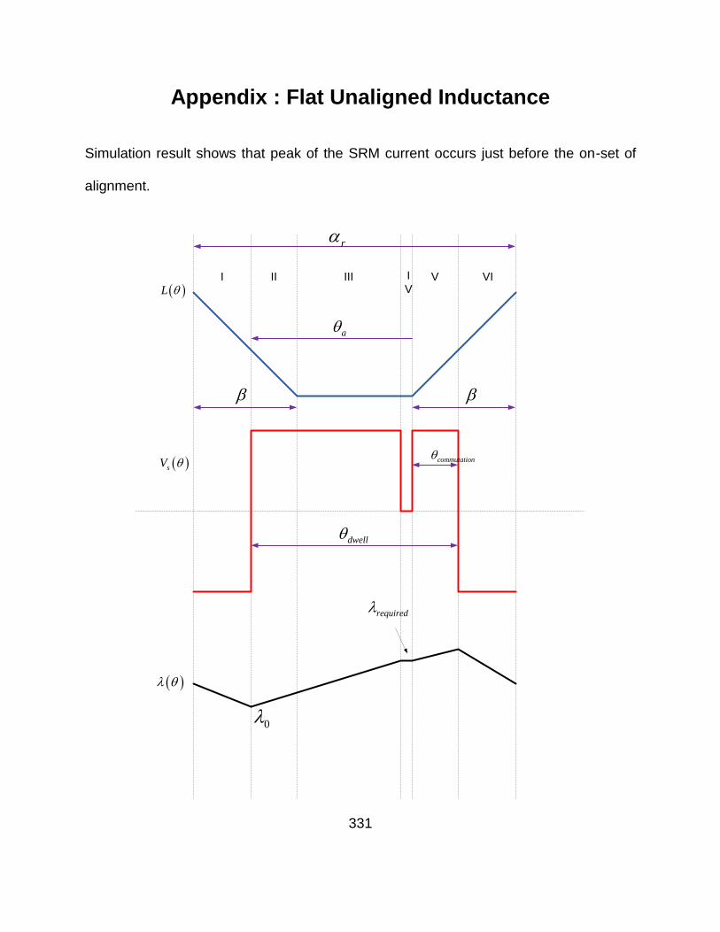
331

Appendix : Flat Unaligned Inductance

Simulation result shows that peak of the SRM current occurs just before the on-set of

alignment.

required

0

I II III I

VV VI

a

r

commutation

dwell

L

sV

332

During transient state : Flux linkage starts with zero value. Since fluxing-region is

greater than de-fluxing region, it does not return back to the same initial value. At what

0 or peak , system achieves steady state ?One way to find this is based on peak

current requirement. Let peakI be the peak current required. We have,

*required peakI L

Simulation results show that the peak current occurs just before the on-set of

alignment. Therefore uL L .Therefore, *required peak uI L .

For 600peakI A and 4.15uL mH , we need 3600*4.15*10 2.49required Wb.

Assume, advance angle, a is given.

Notch length will be : 2* 2*2

rdwell dwell r

Fluxing region duration will be : 2*a dwell r

We have,

0

0

0

0

* 2* ,

* 2* ,

* * 2* ,

* * 2*

srequired a dwell r

srequired a dwell r

su peak a dwell r

su peak a r dwell

Vy mx c

V

VL I

VL I

(1.1)

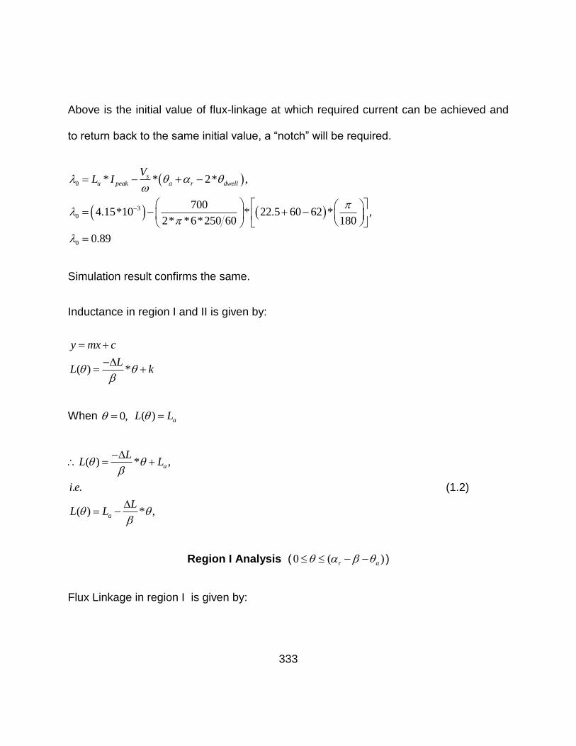
333

Above is the initial value of flux-linkage at which required current can be achieved and

to return back to the same initial value, a “notch” will be required.

0

3

0

0

* * 2* ,

7004.15*10 * 22.5 60 62 * ,

2* *6*250 60 180

0.89

su peak a r dwell

VL I

Simulation result confirms the same.

Inductance in region I and II is given by:

( ) *

y mx c

LL k

When 0, ( ) aL L

( ) * ,

. .

( ) * ,

a

a

LL L

i e

LL L

(1.2)

Region I Analysis (0 ( )r a )

Flux Linkage in region I is given by:

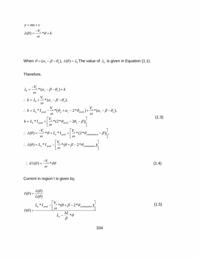
334

( ) *s

y mx c

Vk

When ( ),r a 0( ) The value of 0 is given in Equation (1.1).

Therefore,

0

0

*( )

*( ),

* * 2* *( ),

* *(2* 2 )

( ) * * *(2* ) ,

( ) * *( 2*

sr a

sr a

s su peak a r dwell r a

su peak dwell a

s su peak commutation

su peak c

Vk

Vk

V Vk L I

Vk L I

V VL I

VL I

)ommutation

(1.3)

( ) *sVd d

(1.4)

Current in region I is given by,

( )( )

( )

* *( 2* )

( )

*

su peak commutation

a

IL

VL I

IL

L

(1.5)

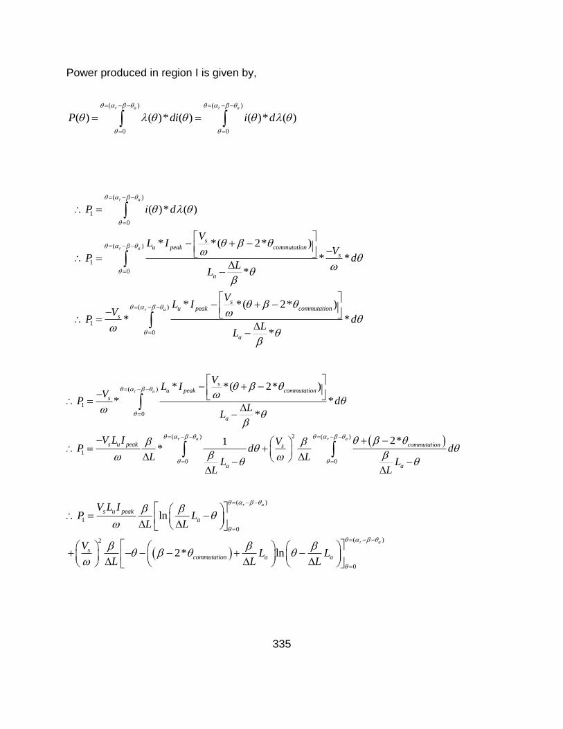
335

Power produced in region I is given by,

( ) ( )

0 0

( ) ( )* ( ) ( )* ( )r a r a

P di i d

( )

1

0

( )

1

0

( )

1

0

( )* ( )

* *( 2* )

* *

*

* *( 2* )

* *

*

r a

r a

r a

su peak commutation

s

a

su peak commutation

s

a

P i d

VL I

VP d

LL

VL I

VP d

LL

( )

1

0

2( ) ( )

1

0 0

* *( 2* )

* *

*

2*1*

r a

r a r a

su peak commutation

s

a

s u peak commutations

a a

VL I

VP d

LL

V L I VP d d

L LL L

L L

( )

1

0

( )2

0

ln

2* ln

r a

r a

s u peak

a

scommutation a a

V L IP L

L L

VL L

L L L

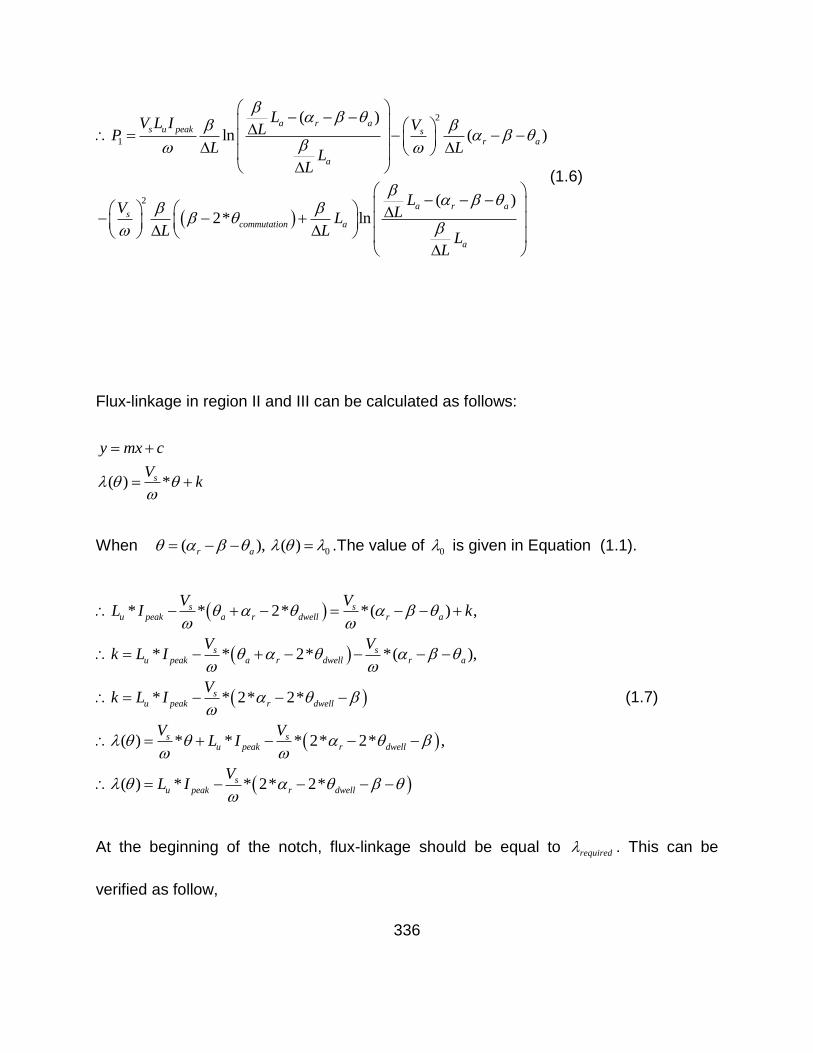
336

2

1

2

( )ln ( )

( )2* ln

a r as u peak s

r a

a

a r as

commutation a

a

LV L I VLPL L

LL

LV LL

L LL

L

(1.6)

Flux-linkage in region II and III can be calculated as follows:

( ) *s

y mx c

Vk

When ( ),r a 0( ) .The value of 0 is given in Equation (1.1).

* * 2* *( ) ,

* * 2* *( ),

* * 2* 2*

( ) * * * 2* 2* ,

( ) * * 2* 2*

s su peak a r dwell r a

s su peak a r dwell r a

su peak r dwell

s su peak r dwell

su peak r dwell

V VL I k

V Vk L I

Vk L I

V VL I

VL I

(1.7)

At the beginning of the notch, flux-linkage should be equal to required . This can be

verified as follow,

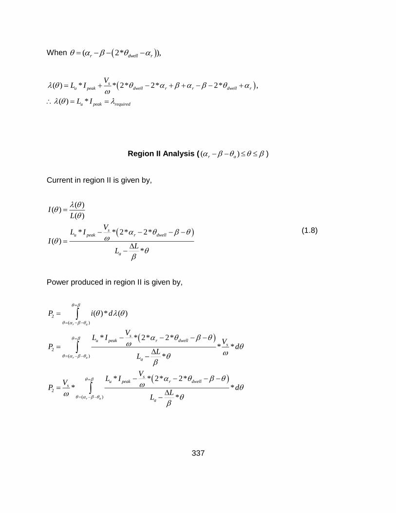
337

When ( 2* ),r dwell r

( ) * * 2* 2* 2* ,

( ) *

su peak dwell r r dwell r

u peak required

VL I

L I

Region II Analysis ( ( )r a )

Current in region II is given by,

( )( )

( )

* * 2* 2*

( )

*

su peak r dwell

a

IL

VL I

IL

L

(1.8)

Power produced in region II is given by,

2

( )

2

( )

2

( )

( )* ( )

* * 2* 2*

* *

*

* * 2* 2*

* *

*

r a

r a

r a

su peak r dwell

s

a

su peak r dwell

s

a

P i d

VL I

VP d

LL

VL I

VP d

LL

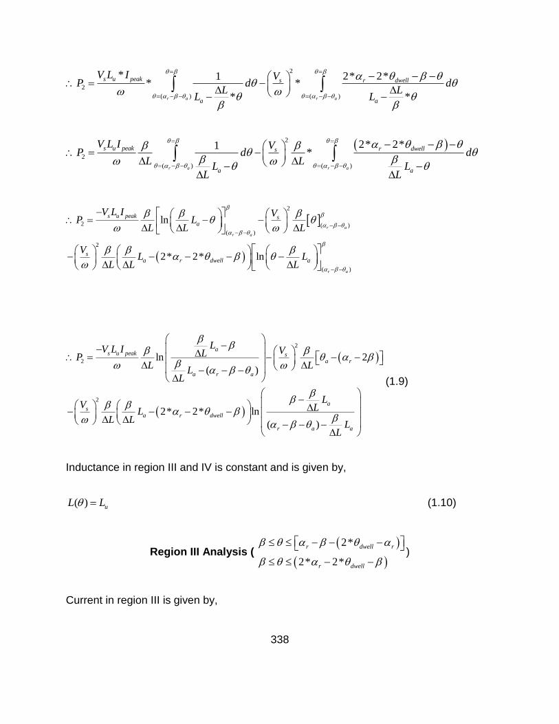
338

2

2

( ) ( )

* 2* 2*1* *

* *r a r a

s u peak s r dwell

a a

V L I VP d d

L LL L

2

2

( ) ( )

2* 2*1*

r a r a

s u peak r dwells

a a

V L I VP d d

L LL L

L L

2

2 ( )

( )

2

( )

ln

2* 2* ln

r a

r a

r a

s u peak sa

sa r dwell a

V L I VP L

L L L

VL L

L L L

2

2

2

ln 2

( )

2* 2* ln

( )

as u peak s

a r

a r a

as

a r dwell

r a a

LV L I VLPL L

LL

LV LL

L LL

L

(1.9)

Inductance in region III and IV is constant and is given by,

( ) uL L (1.10)

Region III Analysis (

2*

2* 2*

r dwell r

r dwell

)

Current in region III is given by,

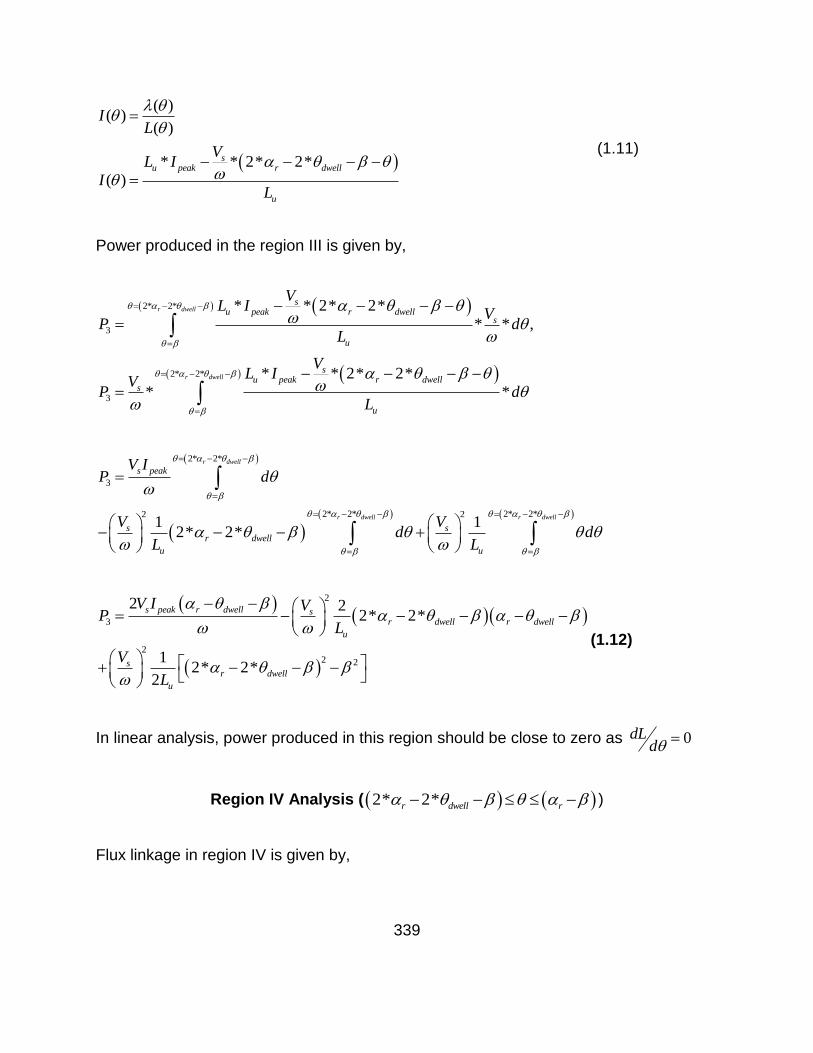
339

( )( )

( )

* * 2* 2*

( )

su peak r dwell

u

IL

VL I

IL

(1.11)

Power produced in the region III is given by,

2* 2*

3

2* 2*

3

* * 2* 2*

* * ,

* * 2* 2*

* *

r dwell

r dwell

su peak r dwell

s

u

su peak r dwell

s

u

VL I

VP d

L

VL I

VP d

L

2* 2*

3

2* 2* 2* 2*2 21 1

2* 2*

r dwell

r dwell r dwell

s peak

s sr dwell

u u

V IP d

V Vd d

L L

2

3

22 2

2 22* 2*

12* 2*

2

s peak r dwell sr dwell r dwell

u

sr dwell

u

V I VP

L

V

L

(1.12)

In linear analysis, power produced in this region should be close to zero as 0dLd

Region IV Analysis ( 2* 2*r dwell r )

Flux linkage in region IV is given by,

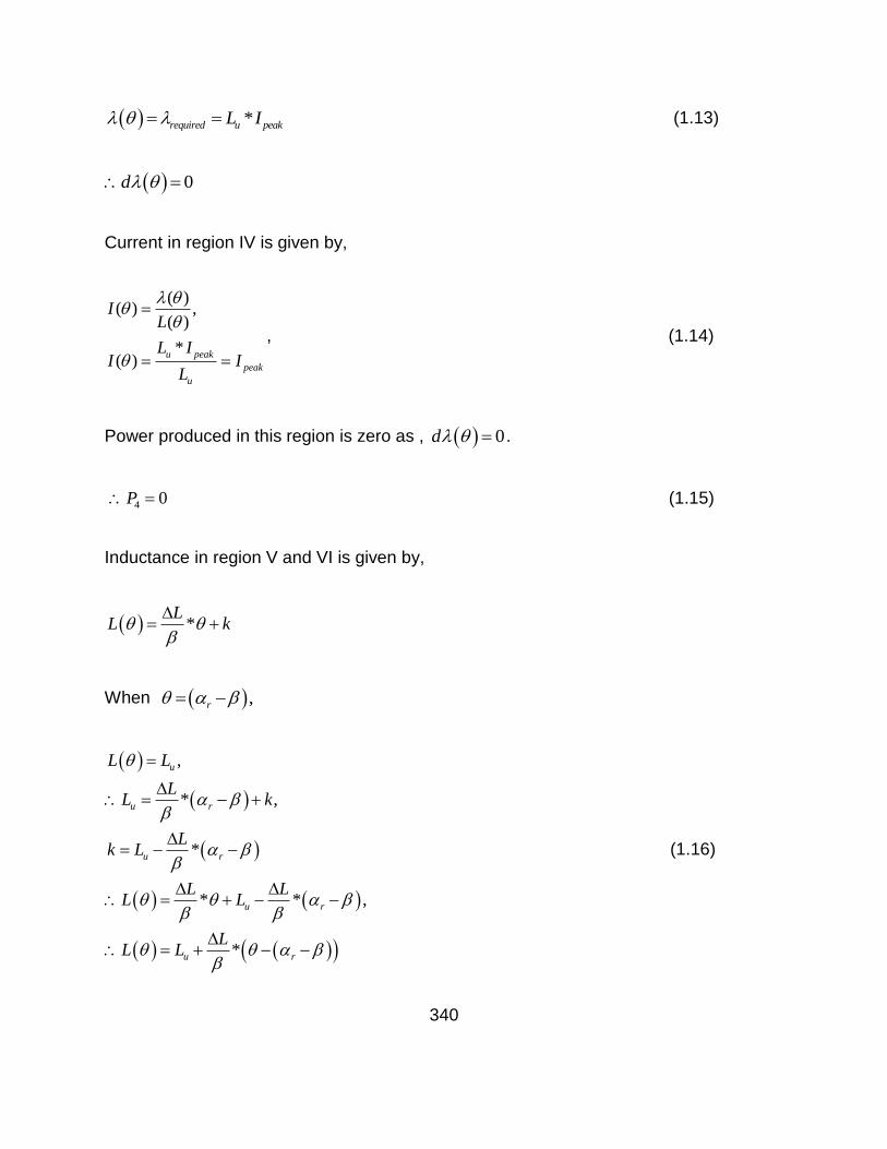
340

*required u peakL I (1.13)

0d

Current in region IV is given by,

( )( ) ,

( )

*( )

u peak

peak

u

IL

L II I

L

, (1.14)

Power produced in this region is zero as , 0d .

4 0P (1.15)

Inductance in region V and VI is given by,

*L

L k

When ,r

,

* ,

*

* * ,

*

u

u r

u r

u r

u r

L L

LL k

Lk L

L LL L

LL L

(1.16)

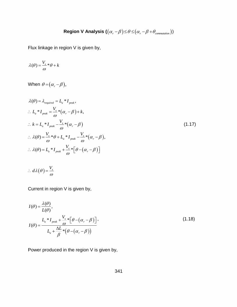
341

Region V Analysis ( r r commutation )

Flux linkage in region V is given by,

( ) *sVk

When ,r

( ) * ,

* * ,

* *

( ) * * * ,

( ) * *

required u peak

su peak r

su peak r

s su peak r

su peak r

L I

VL I k

Vk L I

V VL I

VL I

(1.17)

sVd

Current in region V is given by,

( )( ) ,

( )

* *

( )

*

su peak r

u r

IL

VL I

IL

L

, (1.18)

Power produced in the region V is given by,

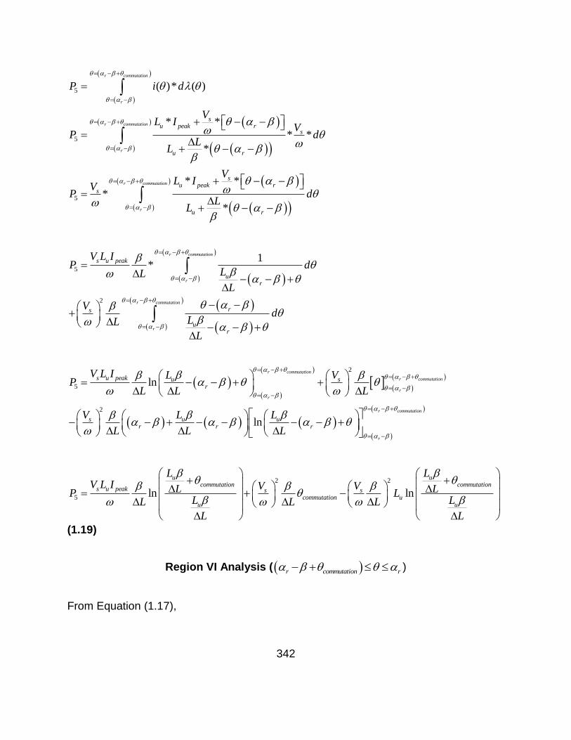
342

5

5

5

( )* ( )

* *

* *

*

* *

*

*

r commutation

r

r commutation

r

r commutation

r

su peak r

s

u r

su peak r

s

u r

P i d

VL I

VP d

LL

VL I

VP d

LL

5

2

1*

r commutation

r

r commutation

r

s u peak

ur

rs

ur

V L IP d

LL

L

Vd

LL

L

2

5

2

ln

ln

r commutation

r commutation

r

r

r commutation

r

s u peak u sr

s u ur r r

V L I L VP

L L L

V L L

L L L

2 2

5 ln ln

u ucommutation commutation

s u peak s scommutation u

u u

L LV L I V VL LP L

L LL L L

L L

(1.19)

Region VI Analysis ( r commutation r )

From Equation (1.17),

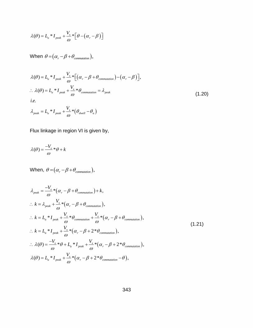
343

( ) * *su peak r

VL I

When ,r commutation

( ) * * ,

( ) * *

. .

* *

su peak r commutation r

su peak commutation peak

speak u peak dwell a

VL I

VL I

i e

VL I

(1.20)

Flux linkage in region VI is given by,

( ) *sVk

When, ,r commutation

* ,

* ,

* * * ,

* * 2* ,

( ) * * * 2* ,

( )

speak r commutation

speak r commutation

s su peak commutation r commutation

su peak r commutation

s su peak r commutation

Vk

Vk

V Vk L I

Vk L I

V VL I

* * 2* ,su peak r commutation

VL I

(1.21)

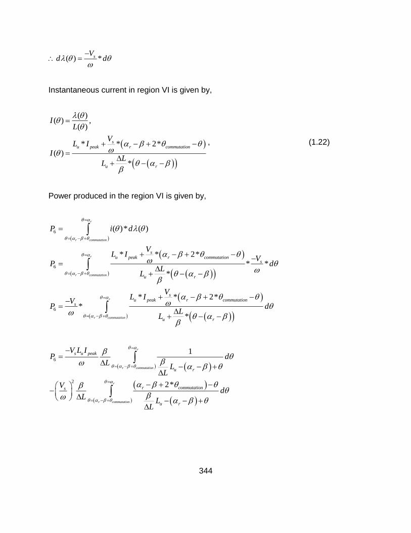
344

( ) *sVd d

Instantaneous current in region VI is given by,

( )( ) ,

( )

* * 2*

( )

*

su peak r commutation

u r

IL

VL I

IL

L

, (1.22)

Power produced in the region VI is given by,

6

6

6

( )* ( )

* * 2*

* *

*

* * 2*

*

*

r

r commutation

r

r commutation

r

r commutation

su peak r commutation

s

u r

su peak r commutation

s

u r

P i d

VL I

VP d

LL

VL I

VP d

LL

6

2

1

2*

r

r commutation

r

r commutation

s u peak

u r

r commutations

u r

V L IP d

LL

L

Vd

LL

L

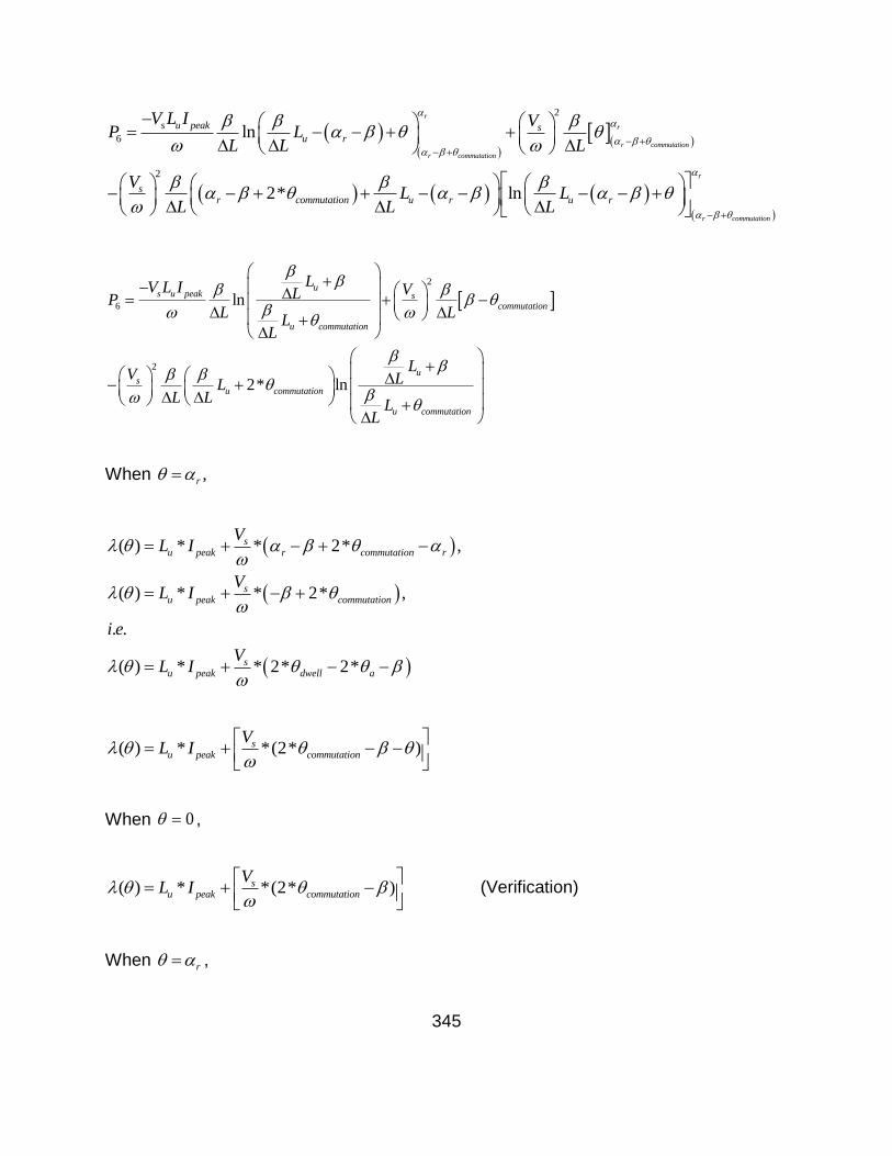
345

2

6

2

ln

2* ln

r

r

r commutation

r commutation

r

r commutation

s u peak su r

sr commutation u r u r

V L I VP L

L L L

VL L

L L L

2

6

2

ln

2* ln

us u peak s

commutation

u commutation

us

u commutation

u commutation

LV L I VLPL L

LL

LV LL

L LL

L

When ,r

( ) * * 2* ,

( ) * * 2* ,

. .

( ) * * 2* 2*

su peak r commutation r

su peak commutation

su peak dwell a

VL I

VL I

i e

VL I

( ) * *(2* )su peak commutation

VL I

When 0 ,

( ) * *(2* )su peak commutation

VL I

(Verification)

When r ,

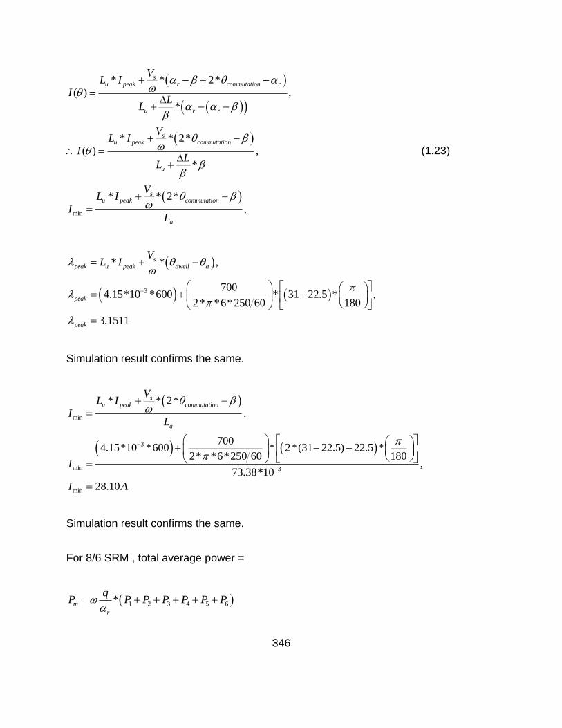
346

min

* * 2*

( ) ,

*

* * 2*

( ) ,

*

* * 2*

,

su peak r commutation r

u r r

su peak commutation

u

su peak commutation

a

VL I

IL

L

VL I

IL

L

VL I

IL

(1.23)

3

* * ,

7004.15*10 *600 * 31 22.5 * ,

2* *6*250 60 180

3.1511

speak u peak dwell a

peak

peak

VL I

Simulation result confirms the same.

min

3

min 3

min

* * 2*

,

7004.15*10 *600 * 2*(31 22.5) 22.5 *

2* *6*250 60 180,

73.38*10

28.10

su peak commutation

a

VL I

IL

I

I A

Simulation result confirms the same.

For 8/6 SRM , total average power =

1 2 3 4 5 6*m

r

qP P P P P P P

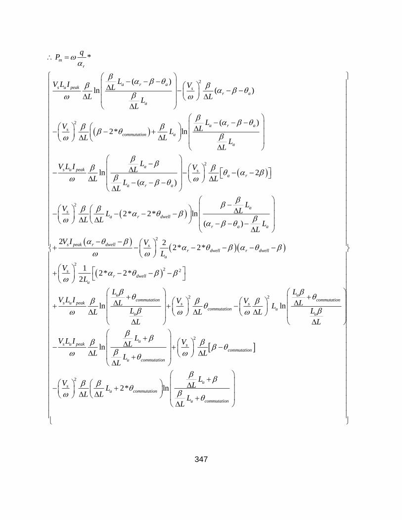
347

2

2

*

( )ln ( )

( )2* ln

ln

( )

m

r

a r as u peak s

r a

a

a r as

commutation a

a

as u peak

a r a

qP

LV L I VL

L LL

L

LV LL

L LL

L

LV L I L

LL

L

2

2

2

22 2

2

2* 2* ln

( )

2 22* 2*

12* 2*

2

sa r

as

a r dwell

r a a

s peak r dwell sr dwell r dwell

u

sr dwell

u

V

L

LV LL

L LL

L

V I V

L

V

L

2 2

2

ln ln

ln

u ucommutation commutation

s u peak s scommutation u

u u

us u peak s

commuta

u commutation

L LV L I V VL LL

L LL L L

L L

LV L I VL

L LL

L

2

2* ln

tion

us

u commutation

u commutation

LV LL

L LL

L

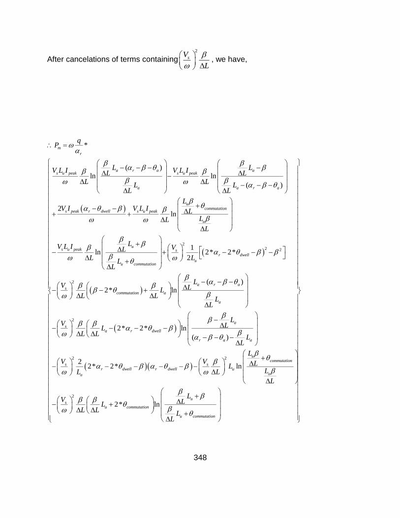
348

After cancelations of terms containing

2

sV

L

, we have,

*

( )ln ln

( )

2ln

ln

m

r

a r a as u peak s u peak

a a r a

ucommutation

s peak r dwell s u peak

u

us u peak

u

qP

L LV L I V L IL L

L LL L

L L

LV I V L I L

LL

L

LV L I L

LL

L

22 2

2

2

12* 2*

2

( )2* ln

2* 2* ln

( )

sr dwell

ucommutation

a r as

commutation a

a

as

a r dwell

r a a

V

L

LV LL

L LL

L

LV LL

L LL

L

2 2

2

22* 2* ln

2* ln

ucommutation

s sr dwell r dwell u

uu

us

u commutation

u commutation

LV V LL

LL L

L

LV LL

L LL

L

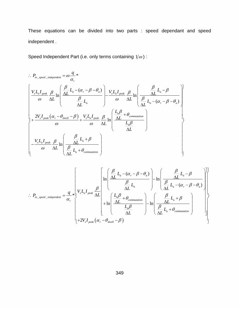
349

These equations can be divided into two parts : speed dependant and speed

independent .

Speed Independent Part (i.e. only terms containing 1 ) :

_ _ *

( )ln ln

( )

2ln

m speed independent

r

a r a as u peak s u peak

a a r a

ucommutation

s peak r dwell s u peak

u

s u peak

qP

L LV L I V L IL L

L LL L

L L

LV I V L I L

LL

L

V L I

lnu

u commutation

LL

LL

L

_ _

( )ln ln

( )

*

ln ln

a r a a

a a r a

s u peak

um speed independentcommutation ur

uu commutation

L LL L

L LL L

V L IqL LP

LL L

LL

LL

2 s peak r dwellV I

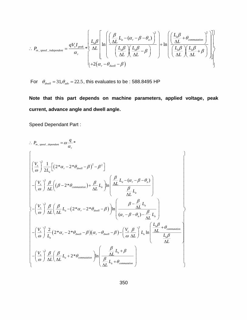
350

22

_ _

( )

ln ln*

2

ucommutationa r a

u

s peaka a u um speed independent

r

r dwell

LL

L LLqV I

L L L LLP

L L L L

For 31, 22.5dwell adv , this evaluates to be : 588.8495 HP

Note that this part depends on machine parameters, applied voltage, peak

current, advance angle and dwell angle.

Speed Dependant Part :

_ _

22 2

2

2

*

12* 2*

2

( )2* ln

2* 2* ln

( )

m speed dependant

r

sr dwell

u

a r as

commutation a

a

as

a r dwell

r a

qP

V

L

LV LL

L LL

L

LV LL

L LL

L

2 2

2

22* 2* ln

2* ln

a

ucommutation

s sr dwell r dwell u

uu

us

u commutation

u commutation

LV V LL

LL L

L

LV LL

L LL

L

351

This can be rewritten as:

2

_ _

2 2

*

12 2

2

( )2 ln

2 2 ln

( )

22 2

s

m speed dependant

r

r dwell

u

a r a

commutation a

a

a

a r dwell

r a a

r dwell r

u

q VP

L

LLL

L LL

L

LLL

L LL

L

L

2

ln

2 ln

ucommutation

dwell uu

u

u commutation

u commutation

L

LLLL

L

LLL

L LL

L

Note that this part does not depend on peak current requirement.

Since 2* * *

60

bn N , at higher speeds, i.e. as n ,

22

2 22 2

( )

ln lnlim *

2

ucommutationa r a

u

s peak

m a a u u

r

r dwell

LL

L LLqV I

LP L L L L

L L L L

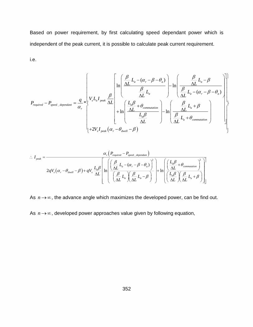
352

Based on power requirement, by first calculating speed dependant power which is

independent of the peak current, it is possible to calculate peak current requirement.

i.e.

_

( )ln ln

( )

*

ln ln

a r a a

a a r a

s u peak

urequired speed dependantcommutation ur

uu commutation

L LL L

L LL L

V L IqL LP P

LL L

LL

LL

2 s peak r dwellV I

_

22

( )

2 ln ln

r required speed dependant

peak

ucommutationa r a

us r dwell s

ua a u

P PI

LL

L LLqV qV

LLL L L

L L L L

As n , the advance angle which maximizes the developed power, can be find out.

As n , developed power approaches value given by following equation,

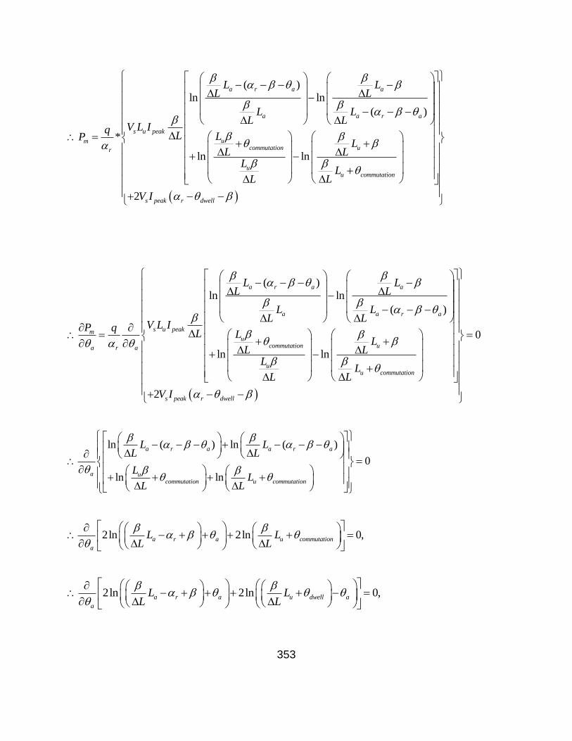
353

( )ln ln

( )

*

ln ln

2

a r a a

a a r a

s u peak

umcommutation ur

uu commutation

s peak r dwel

L LL L

L LL L

V L IqL LP

LL L

LL

LL

V I

l

( )ln ln

( )

ln ln

2

a r a a

a a r a

s u peakmu

commutation ua r a

uu commutation

s peak

L LL L

L LL L

V L IP qL L

LL L

LL

LL

V I

0

r dwell

ln ( ) ln ( )

0

ln ln

a r a a r a

a ucommutation u commutation

L LL L

LL

L L

2ln 2ln 0,a r a u commutation

a

L LL L

2ln 2ln 0,a r a u dwell a

a

L LL L

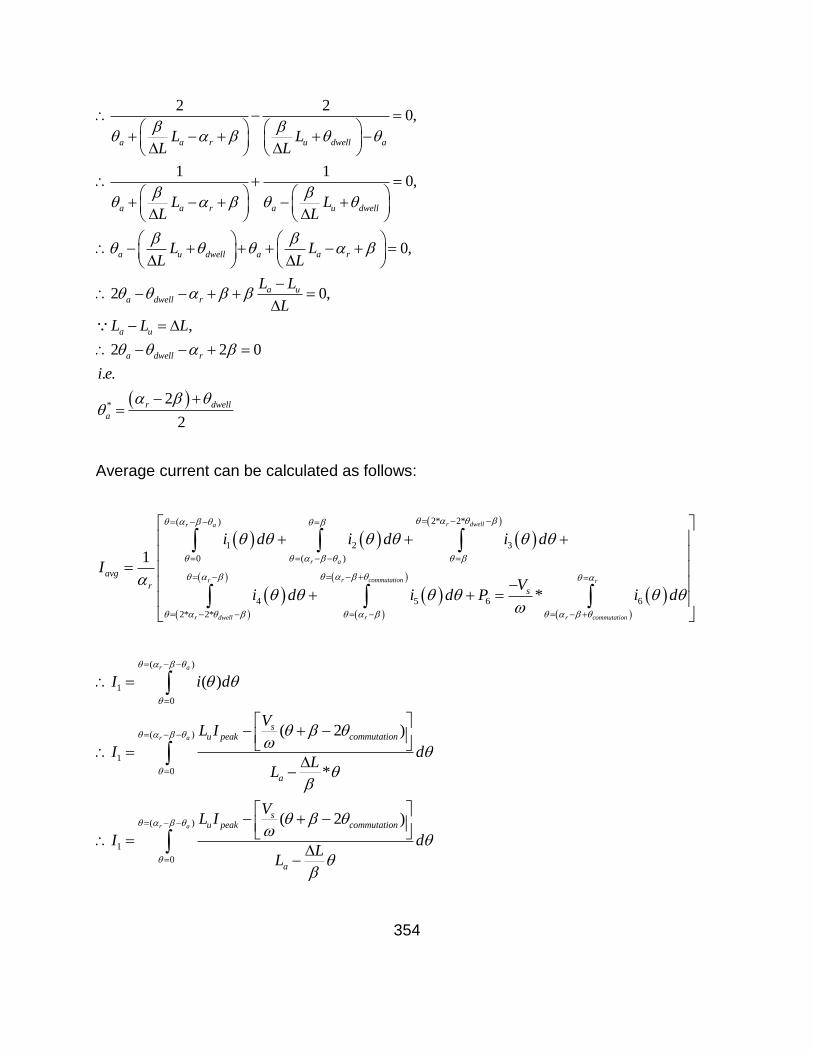
354

2 20,

1 10,

0,

2 0,

,

2 2 0

. .

a a r u dwell a

a a r a u dwell

a u dwell a a r

a ua dwell r

a u

a dwell r

L LL L

L LL L

L LL L

L L

L

L L L

i e

*2

2

r dwell

a

Average current can be calculated as follows:

2* 2*( )

1 2 3

0 ( )

4 5 6 6

2* 2*

1

*

r dwellr a

r a

r commutationr r

r dwell r r commutation

avg

rs

i d i d i d

IV

i d i d P i d

( )

1

0

( )

1

0

( )

1

0

( )

( 2 )

*

( 2 )

r a

r a

r a

su peak commutation

a

su peak commutation

a

I i d

VL I

I dL

L

VL I

I dL

L

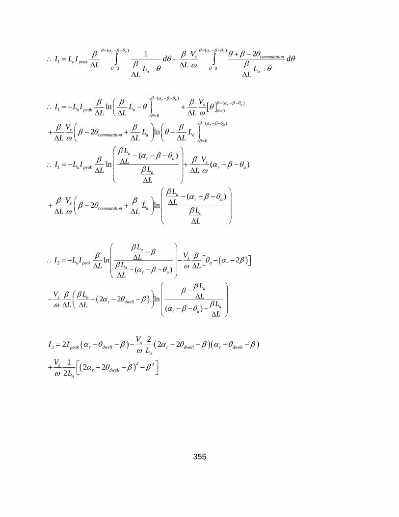
355

( ) ( )

1

0 0

21r a r a

s commutationu peak

a a

VI L I d d

L LL L

L L

( )

( )

1 00

( )

0

1

ln

2 ln

( )ln ( )

r a

r a

r a

su peak a

scommutation a a

ar a

su peak r a

a

s

VI L I L

L L L

VL L

L L L

LVLI L I

LL L

L

V

L

( )2 ln

ar a

commutation aa

L

LLLL

L

2 ln 2

( )

2 2 ln

( )

a

su peak a r

ar a

a

s ar dwell

ar a

LVLI L I

LL L

L

LV L L

LL L

L

3

2 2

22 2 2

12 2

2

speak r dwell r dwell r dwell

u

sr dwell

u

VI I

L

V

L

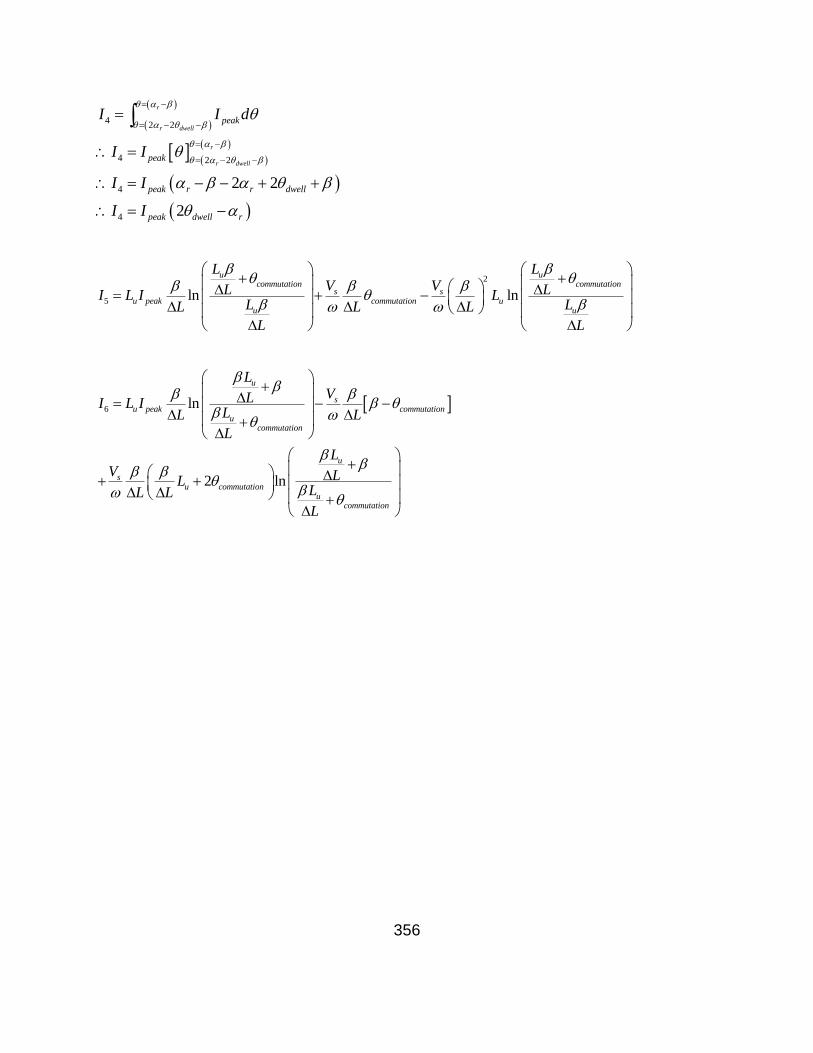
356

42 2

4 2 2

4

4

2 2

2

r

r dwell

r

r dwell

peak

peak

peak r r dwell

peak dwell r

I I d

I I

I I

I I

2

5 ln ln

u ucommutation commutation

s su peak commutation u

u u

L LV VL LI L I L

L LL L L

L L

6 ln

2 ln

u

su peak commutation

ucommutation

u

su commutation

ucommutation

LVLI L I

LL L

L

LV LL

LL L

L

357

( )ln ( )

( )2 ln

ln 2

( )

1

ar a

su peak r a

a

ar a

scommutation a

a

a

su peak a r

ar a

s

avg

r

LVLL I

LL L

L

LV LL

LL L

L

LVLL I

LL L

L

V

I

2 2

2 2 ln

( )

22 2 2

12 2 2

2

ln

a

ar dwell

ar a

speak r dwell r dwell r dwell

u

sr dwell peak dwell r

u

ucommutation

u peaku

LL L

LL L

L

VI

L

VI

L

L

LL ILL

L

2

ln

ln

2 ln

ucommutation

s scommutation u

u

u

su peak commutation

ucommutation

u

su commutation

ucommutatio

LV V LL

LL L

L

LVLL I

LL L

L

LV LL

LL L

L

n

Again this can be split into Speed Dependent part and Speed Independent part.

358

_ _

( )ln ln

( )

12 2

ln

a ar a

u peak u peaka a

r a

avg speed independent peak r dwell peak dwell r

r

ucommutation

u peak u peu

L L

L LL I L IL LL L

L L

I I I

L

LL I L ILL

L

ln

u

aku

commutation

L

LLL

L

_ _ ln 2

a u

peak uavg speed independent r

u ar

L L

I L L LI

L LL

L L

359

_ _

( ) 2

( )2 ln

2 2 ln

( )

1

s s sr a a r commutation

ar a

s acommutation

a

a

s ar dwell

ar a

avg speed dependent

r

V V V

L L L

LV L L

LL L

L

LV L L

LL L

I

2 2

2

22 2

12 2

2

ln

2 ln

sr dwell r dwell

u

sr dwell

u

ucommutation

s scommutation u

u

u

su commutation

ucommutation

L

V

L

V

L

LV V LL

LL L

L

LV LL

LL L

L

360

_ _

( )2 ln

2 2 ln

( )

ln

2

ar a

acommutation

a

a

ar dwell

ar a

ucommutation

us

avg speed dependentu

r

uco

LL L

LL

L

LL L

LL

L

LL LV

I LLLL

L

L

2 2

ln

22 2

2 2 (2 4 4 2 )2

u

mmutationu

commutation

r dwell r dwell

u

r dwell r a d

u

L

LL

L

L

L

L

L

As speed increases, i.e. n ,

lim ln 2

a u

peak uavg r

u ar

L L

I L L LI

L LL

L L

And developed power,

22

2 22 2

( )

ln lnlim *

2

ucommutationa r a

u

s peak

m a a u u

r

r dwell

LL

L LLqV I

LP L L L L

L L L L

361

This power can be optimized using, *

2

2

r dwell

a

.

362

Vita

Niranjan Anandrao Patil was raised in Shirala (Maharashtra,India). He graduated from

PVP Institute of Technology with honors, in year 2000 and received a B.Eng. in

Instrumentation and Control. He then worked for an automation firm as a Project

Engineer (Distributed Control Systems) for two years. There, he worked on three

projects involving automation of metal and chemical industries.

He joined the University of Tennessee, Knoxville in year 2002 and received a M.S. in

Electrical Engineering in December 2004. During his M.S., he worked at Office of

Information and Technology as Graduate Assistant. In 2005, he started his Ph.D.

During his Ph.D., he worked with National Transportation Research Center as a

Research Assistant. He also received a Teaching Assistantship from the ECE

department.

In 2008, he worked part-time for MESA Inc. in Knoxville, TN as an Electrical Engineer.

There, he was responsible for electrical distribution analysis. His professional interest

includes process instrumentation and control; electrical drives and control; power

system analysis and control. He is currently working as Drives and Power System

Engineer with GE Industrial Automation division. He is a member of ISA and IEEE.