Embed Size (px)
Citation preview

Journal of the Japanese and International Economies 16, 405–435 (2002)doi:10.1006/jjie.2002.0514
To Spend the U.S. Government Surplus or to Increase theDeficit? A Numerical Analysis of the Policy Options1
Stephen J. Turnovsky
Department of Economics, University of Washington, Seattle, Washington
and
Santanu Chatterjee
Department of Economics, Terry College of Business, University of Georgia, Atlanta, Georgia
Received January 18, 2002; revised September 8, 2002
Turnovsky, Stephen J., and Chatterjee, Santanu—To Spend the U.S. Government Sur-plus or to Increase the Deficit? A Numerical Analysis of the Policy Options
This paper provides a numerical analysis of the likely benefits from adopting alterna-tive ways of reducing the projected fiscal surplus (as of the summer 2001) in the UnitedStates economy. Calibrating a small growth model, our results suggest that investing thesurplus in public capital is likely to yield the greatest long-run welfare gains, althoughdecreasing the capital income tax is only marginally inferior. Both these options dominateincreasing government consumption expenditure or decreasing the tax on labor income.By shifting resources from consumption toward capital the two superior policies involvesharp intertemporal tradeoffs in welfare; significant short-run welfare losses are more thancompensated by large long-run welfare gains. By contrast, the two inferior options aregradually welfare-improving through time. A crucial factor in determining the benefits ofreducing the government surplus through spending is the size of the government sectorrelative to the social optimum. We find that the second-best optimum is to increase bothforms of government expenditure to their respective social optima, while at the same timerestructuring taxes by reducing the tax on capital and raising the tax on wage income toachieve the targeted reduction in the surplus. J. Japan. Int. Econ., December 2002, 16(4),pp. 405–435. Department of Economics, University of Washington, Seattle, Washington;
1 This is a revised version of a paper presented at the 14th Annual NBER-CEPR-TCER Conferenceon Issues in Fiscal Adjustment, held in Tokyo, December 13–14, 2001. The comments of the discussantsShin’ichi Fukuda, Toshihiro Ihori, and an anonymous referee are gratefully acknowledged.
405
0889-1583/02 $35.00c© 2002 Elsevier Science (USA)
All rights reserved.

406 TURNOVSKY AND CHATTERJEE
and Department of Economics, Terry College of Business, University of Georgia, Atlanta,Georgia. c© 2002 Elsevier Science (USA)
Journal of Economic Literature Classification Numbers: E62, O41.
Key Words: Government surplus; Policy options.
1. INTRODUCTION
During the summer of 2001 the U.S. government was projecting substantialgovernment surpluses at least for the medium-term future. On the basis of theseprojections the Bush administration had proposed a 1.6 trillion dollar tax cut tobe phased in over 10 years, an amount that eventually was trimmed slightly to1.5 trillion dollars. The tragic events of September 11, 2001, together with thedecline in activity already in process, have cast serious doubts on the accuracy ofthe earlier projections with the likelihood that the debate will be revisited, this timeunder a less rosy scenario.2 But whether one is talking about reducing (spending)a projected budget surplus or financing by deficit spending, the principle is thesame. We shall therefore carry out our discussion in terms of the surplus, eventhough that situation is now much more in doubt.
The allocation of the projected budget surplus in the United States generated aspirited debate among policymakers and academic researchers, particularly duringthe spring of 2001. Basically three broad options are available: (i) to reduce the out-standing debt, (ii) to spend the surplus on new government expenditure programs,and (iii) to reduce tax rates. Options (ii) and (iii) contain several suboptions. Onecritical policy choice concerns the form that a proposed increase in governmentexpenditure should take. Whether an increase in government expenditure takes theform of some publicly provided consumption good or the form of public invest-ment that enhances the productive capacity of the economy is an important policychoice. Likewise, the nature of the tax cuts, whether they are targeted toward laborincome or capital income, or are applied uniformly to both, is also a key policydecision.3
It is clear that different government policies will differ dramatically from oneanother in terms of the growth paths they generate, the timing of the benefits theyyield, and their distributional impacts across the economy. Both forms of gov-ernment expenditure crowd out private consumption, leading to short-run welfarelosses. But the private consumption losses incurred in the case of governmentconsumption expenditure are more than offset by the direct benefits provided bythe latter, yielding overall welfare gains in the short run. In contrast, government
2 Indeed, during the winter of 2002 the U.S. Congress was again debating an economic stimuluspackage in response to the prevailing economic downturn.
3 Another issue that has been discussed periodically with some vigor is the idea of replacing theincome tax with a consumption tax. Since this is not part of the current discussion, we do not addressit here. This policy has been analyzed by Turnovsky (2001).
TO SPEND THE U.S. SURPLUS OR INCREASE THE DEFICIT 407
investment expenditure yields no consumption benefits in the short run. Instead,these resources devoted to increasing the economy’s productive capacity lead togreater consumption benefits in the longer run. Likewise, cutting the tax on cap-ital income is likely to have a greater positive impact on the immediate growthperformance of the economy than does a tax cut directed toward labor income.
To analyze these issues requires a carefully specified dynamic macro model.The objective of this paper, therefore, is to apply such a model to characterizingand evaluating the differential effects of such alternative policies on the transi-tional adjustment path of an economy faced with a large initial budget surplus.The basic model we apply has been developed by Turnovsky (2001). The keycomponents of the model are that it is a one-sector growth model in which outputdepends upon the stocks of both private and public capital, as well as endogenouslysupplied labor. The production function is sufficiently general to allow the econ-omy to have increasing or decreasing returns to scale in the aggregate. In additionto accumulating public capital, the government allocates resources to a utility-enhancing consumption good. These expenditures are financed by issuing bonds,distortionary taxes levied on capital income and labor income, or by imposingnondistortionary lump-sum taxation (equivalent to debt).
The model is a nonscale growth model of the type developed by Jones (1995a,1995b) and Young (1998).4 These models, which can also be viewed as extensionsof the standard Solow–Swan neoclassical growth model, have the characteristicthat the long-run growth rate is independent of the size (scale) of the economy,thereby eliminating a counterfactual aspect of many endogenous growth models;see Backus et al. (1992), Easterly and Rebelo (1993), Jones (1995a, 1995b), Stokeyand Rebelo (1995). One of the features of the two-capital good model, again broadlyconsistent with the empirical evidence, is that it is characterized by relatively slowspeeds of convergence.5 The significance of this is that the economy spends a largeproportion of its time away from steady state, thereby increasing the importanceof studying the transitional path.6
4 This contrasts with the endogenous growth models, an initially regarded attractive feature of whichwas the key role that they assigned to fiscal policy. However, these models have shortcomings suchas scale effects, knife-edge characteristics, and unsatisfactory dynamic characteristics that make themless attractive for conducting the type of numerical analysis that we are undertaking here. These issuesand the relevant literature are reviewed by Turnovsky (2000, Chapters 13, 14).
5 Benchmark empirical estimates of the speed of convergence obtained by Barro (1991), Barro andSala-i-Martin (1992), and Mankiw et al. (1992) find the speed of convergence to be around 2–3% perannum. Subsequent studies suggest that the convergence rates are more variable and more sensitiveto the time periods and the characteristics of economies, and a wider range of estimates have beenobtained; see Islam (1995), Evans (1996), and Temple (1998). Eicher and Turnovsky (1999) andTurnovsky (2001) obtain asymptotic speeds of convergence consistent with the 2–3% figure, althoughthey also find that in the short run, the speed of convergence may be substantially higher.
6 One further attractive feature of the nonscale model is that it generates a higher order dynamictransition path than does the corresponding endogenous growth model. This has the advantage ofyielding more flexible transitional adjustment paths, consistent with the empirical evidence; see Bernardand Jones (1996a, 1996b).
408 TURNOVSKY AND CHATTERJEE
But the study of the transitional dynamics is not easy. Even in a small modelsuch as this, with two types of capital, it is necessary to analyze it numerically,and in this respect the model is capable of replicating the key stylized facts of abenchmark economy, such as the United States, with relative ease. The focus of themodel is on the impact of policy shocks on the transition paths and to investigatehow these accumulate to yield long-run impacts on capital stocks and welfare.This type of model provides an excellent vehicle for examining the kinds of policyissues enunciated above. For this purpose, we calibrate a benchmark economywith a large initial budget surplus, such as the United States has recently enjoyed,and then assess the differential dynamic effects of various fiscal policy measuresto reduce this surplus intertemporally.7
Using this calibrated economy, we compare the effects on the economy ofadopting the following fiscal policies, each of which reduces the intertemporalbudget surplus (measured in discounted present value terms) by the same specifiedamount:
(i) Increasing the rate of government consumption expenditure by 5 per-centage points;
(ii) increasing the rate of government investment expenditure by 5 percent-age points,
(iii) decreasing the tax rate on capital income by 14 percentage points, and(iv) decreasing the tax rate on labor income by just under 8 percentage points.
Particular attention is focused on two aspects. The first is on the transitional ad-justment paths of key macroeconomic variables such as private and public capital,output, and consumption, as well as the current surplus. The second is on the timepath of instantaneous welfare, as well as on the overall intertemporal welfare of therepresentative agent in the economy. A crucial aspect of evaluating the merits ofdifferent policies aimed at reducing the fiscal surplus involves the assessment of theintertemporal tradeoffs they generate and this is a central feature of our analysis.
The general conclusion we obtain is that to the extent that the calibrated model isrepresentative of the prevailing U.S. situation, the policy responses (i)–(iv) can beranked as follows. Spending the surplus on government investment is best, beingmarginally superior to reducing the tax on capital, which in turn is substantiallybetter than spending the surplus on government consumption or reducing the taxon labor income. Numerically, the welfare gains that range between 2.5 and 3.8%increase in terms of permanent output flows. But there are sharp intertemporaltradeoffs. The first two policies, which yield the most substantial long-run gains,
7 Our approach is related to the early work of Auerbach and Kotlikoff (1987) who conduct a compre-hensive analysis of the dynamics of fiscal policy using simulation methods, though there are importantdifferences. For example, whereas we use the representative agent model, they use a 55-period over-lapping generations model. But the major difference is that we stress the expenditure side, contrastingthe impact of government consumption with government investment expenditure under alternative taxregimes. By contrast, Auerbach and Kotlikoff focus entirely on the revenue side; government expen-diture has no impact on private behavior.

TO SPEND THE U.S. SURPLUS OR INCREASE THE DEFICIT 409
also involve significant short-run losses, as they both involve diverting resourcesfrom consumption in the short run to investment having longer-run and ultimatelygreater payoffs. But these two policies will also lead to economies having sub-stantially different structural characteristics. Spending the surplus on governmentinvestment will lead in the long run to an economy having a much larger ratioof public to private capital than if the surplus is allocated to reducing the cost ofprivate investment, thereby stimulating private investment.
Alternative policy mixes are also discussed. In this respect we find that a uniformincrease in the two types of government expenditure—on consumption and oninvestment—is marginally superior to increasing investment alone. The reason forthis is because both forms of expenditure provide diminishing marginal benefits,and indeed, optimal levels of expenditure for both forms of expenditure exist.We show that welfare can be enhanced even further by setting the two types ofexpenditures at their respective optima, reducing the tax on capital and raising thetax on labor, consistent with reducing the intertemporal government surplus by thespecified target amount.
We should emphasize that the conclusions we draw regarding the relative meritsof the alternative modes of spending the surplus depend crucially upon the sizes ofthe parameters that reflect the benefits of the two forms of government expenditure.While we feel that these plausibly reflect the U.S. parameters, to the extent thatthis is not so, our conclusions would be modified. It is certainly possible for bothforms of government expenditure to be dominated by tax cuts, and indeed even tobe welfare deteriorating in extreme cases.
The remainder of the paper proceeds as follows. Section 2 sets out the analyticalmodel, while Section 3 derives the equilibrium dynamics. Section 4 briefly char-acterizes the first-best optimum, mainly to serve as a benchmark for our choice ofcritical parameter values. Section 5 calibrates the model, while Section 6 discussesthe dynamics of reducing the surplus. Section 7 briefly conducts some sensitivityanalysis and Section 8 reviews our main conclusions.
2. THE MODEL
The economy comprises N identical individuals, with population growing ex-ponentially at the steady rate N = nN . Each representative agent has an infiniteplanning horizon and possesses perfect foresight. He is endowed with a unit oftime that can be allocated either to leisure, li , or to labor, (1 − li ), and producesoutput, Yi , using the Cobb–Douglas production function
yi = α(1 − li )1−σ K σ
i K η
G 0 < σ < 1, η > 0, (1a)
where Ki denotes the agent’s individual stock of private capital, and KG is thestock of government capital, such as infrastructure. We assume that the servicesderived from the latter are not subject to congestion, so that KG is a pure publicgood, generating a positive externality, parameterized by η. The producer faces
410 TURNOVSKY AND CHATTERJEE
constant returns to scale in the two private factors, and increasing returns to scale,1 + η, in all three factors of production.8
The representative agent’s welfare is specified by the intertemporal isoelasticutility function
� ≡∫ ∞
0(1/γ )
(Cil
θi Hφ
)γe−ρt dt ;
(1b)
φ > 0, θ > 0; −∞ < γ ≤ 1; 1 > γ (1 + φ); 1 > γ (1 + θ + φ),
where C denotes aggregate consumption, so that per capita consumption of theinidividual agent at time t is C/N = Ci , H denotes the consumption services of agovernment-provided consumption good, and the parameters θ and φ measure theimpacts of leisure and public consumption on the agent’s welfare.9 The remainingconstraints on the coefficients appearing in (1b) are imposed in order to ensurethat the utility function is concave in the quantities Ci , li , and H .
The agent’s objective is to maximize (1b) subject to his or her accumulationequation
K i + Bi = [(1 − τk)r − n − δK ]Ki + [(1 − τk)s − n]Bi
+ (1 − τw)w(1 − li ) − Ci − Ti , (1c)
where r is gross return to capital, w is (before-tax) wage rate, s is interest rate ongovernment bonds, the individual’s holdings of which are Bi , τk is tax on capital(and bond) income, τw is tax on wage income, and Ti = T/N is the agent’s shareof lump-sum taxes (transfers). Equation (1c) embodies the assumption that privatecapital depreciates at the rate δK , so that with the growing population the net after-tax private return to capital is (1 − τk)r − n − δK , while the net after-tax return oninterest income is (1 − τk)s − n.
Performing the optimization yields:
Cγ−1i lθγ Hφγ = λi (1 + τc) (2a)
θCγ
i lθγ−1 Hφγ = λiw(1 − τw) (2b)
r (1 − τk) − n − δK = ρ − λi
λi(2c)
r (1 − τk) − δK = s(1 − τk). (2d)
Equation (2a) equates the marginal utility of consumption to the individual’s
8 The assumption that the production function has constant returns to scale in the private factorsof production so that public capital provides a positive externality is a natural one. An alternativeassumption, followed by some authors, is that the production function has constant returns to scale inall three factors of production. One of the advantages of the nonscale model is that it can deal witheither case. The only real restriction is that the externality provided by the public input cannot be toolarge that it violates the stability of the dynamic system (18).
9 The parameter γ is related to the intertemporal elasticity of substitution, e say, by e = 1/(1 − γ ).
TO SPEND THE U.S. SURPLUS OR INCREASE THE DEFICIT 411
tax-adjusted shadow value of wealth, λi , while (2b) equates the marginal util-ity of leisure to its opportunity cost, the after-tax real wage, valued at the shadowvalue of wealth.10 The third equation is the standard Keynes–Ramsey consump-tion rule, equating rate of return on consumption to the after-tax rate of return oncapital, while (2d) equates the net rates of return on the two assets. Finally, in or-der to ensure that the agent’s intertemporal budget constraint is met, the followingtransversality condition must be imposed:
limt→∞ λi Ki e
−ρt = limt→∞ λi Bi e
−ρt = 0. (2e)
Aggregating over the individual production functions, (1a), aggregate output,Y , is
Y = NYi = α[(1 − l)N ]1−σ K σ K η
G, (3)
where K = N Ki denotes aggregate capital. The equilibrium real return to privatecapital and the real wage are thus respectively:
r = ∂Y
∂K= σY
K= σYi
Ki; w = ∂Y
∂[N (1 − l)]= (1 − σ )Y
N (1 − l)= (1 − σ )Yi
(1 − l). (4)
Government capital accumulates in accordance with
K G = G − δG KG, (5)
where G denotes the gross rate of government investment expenditure, and gov-ernment capital depreciates at the rate δG . We assume that the government sets itscurrent gross expenditures on the investment good and the consumption good asfixed fractions of output, namely
G = gY (6a)
H = hY, (6b)
where g, h are chosen policy parameters. A constant government expenditurepolicy is thus associated with a fixed claim on output, and an expenditure levelthat grows with current output, with an expansionary policy being expressed byan increase in the (fixed) fraction. This is an appropriate specification of policy ina growth environment. The government’s fiscal decisions are made subject to itsflow budget constraint
B = (1 − τk)s B + G + H − τkr K − τww(1 − l)N − T, (7)
where B ≡ N Bi denotes the aggregate stock of bonds. Using (6a) and (6b), together
10 Since all agents are identical, each devotes the same fraction of time to leisure, and henceforthwe can drop the agent’s subscript to l.

412 TURNOVSKY AND CHATTERJEE
with the optimality conditions (4) we may express (7) as
B = (1 − τk)s B + [g + h − τkσ − τw(1 − σ )]Y − T . (7′)
Written in this way we see that [g + h − τkσ − τw(1 − σ )]Y specifies the pri-mary budget deficit. Thus, T (t) = [g + h − τkσ − τw(1 − σ )]Y (t) represents theamount of lump-sum taxation (or transfers) necessary to finance the primary deficitand is therefore a measure of current fiscal imbalance; see Bruce and Turnovsky(1999). Defining
V ≡∫ ∞
oT (t)e− ∫ t
0 s(u)(1−τk )du dt (8)
the government’s intertemporal budget constraint, obtained by solving (7′) andimposing the transversality condition, can be written in the form
V = B0 +∫ ∞
0[g + h − τkσ − τw(1 − σ )]Y (t)−
∫ t0 s(u)(1−τk )du dt. (9)
In general we say that the government is operating an intermporally consistentfiscal policy as long as its expenditure and tax rates are such that (9) is satisfiedwith V = 0. Thus V measures the present discounted value of the lump-sum taxesor transfers necessary to balance the budget over time and is thus a measure ofthe intertemporal (im)balance of the government’s budget. We shall focus on thecase where the government is running an intertemporal surplus and the alternativefiscal policies we shall consider are all constrained to reduce the balancing termV by the same amount.
Aggregating (1c) over the N individuals and combining with (7′) leads to theaggregate resource constraint
K = Y − C − G − H − δK K . (10)
Substituting (6a), (6b) into (10), we may write the growth rate of private capitalas:
K
K=
(1 − g − h − C
Y
)Y
K− δK . (11a)
Likewise, substituting (6a) into (5), the growth rate of public capital may be writtenas:
K G
KG= g
Y
KG− δG . (11b)

TO SPEND THE U.S. SURPLUS OR INCREASE THE DEFICIT 413
3. EQUILIBRIUM DYNAMICS
Our objective is to specify the transitional dynamics of the aggregate economyabout a long-run balanced growth path. In long-run equilibrium, aggregate output,private capital, and public capital are assumed to grow at the same constant rate,so that the output–capital ratio and the ratio of public capital to private capitalremain constant, while the fraction of time devoted to leisure remains constant.Taking percentage changes of the aggregate production function, (3), the long-runequilibrium growth rate of output, private and public capital, ψ , is:
ψ =(
1 − σ
1 − σ − η
)n. (12)
We shall show that one condition for the dynamics to be stable is that σ + η < 1,in which case the long-run equilibrium growth rate ψ > 0. As long as governmentcapital is productive, (12) implies that long-run per capita growth, ψ − n, is positiveas well.
To analyze the transitional dynamics of the economy about the long-run sta-tionary growth path, we express the system in terms of the following stationaryvariables: (i) the fraction of time devoted to leisure, l, and (ii) the scale-adjustedper capita quantities11
k ≡ K
N ((1−σ )/(1−σ−η)); kg ≡ KG
N ((1−σ )/(1−σ−η)); y ≡ Y
N ((1−σ )/(1−σ−η)). (13)
Using this notation, the scale-adjusted output can be written as:
y = α(1 − l)1−σ kσ kηg . (14)
Elsewhere we have shown how the equilibrium dynamics can be expressed asthe following system in the redefined stationary variables, l, k, kg:
l = F(l)
{((1 − τk)σ − [1 − γ (1 + φ)]
[σ (1 − c − g − h) + ηgk
kg
])y
k
− δK (1 − σ [1 − γ (1 + φ)]) + δGη[1 − γ (1 + φ)]
− ([(1 − σ )[1 − γ (1 + φ)] + γ ]n + ρ)
}(15a)
k
k= (1 − c − g − h)
y
k− δK − ψ (15b)
11 Under constant returns to scale, these expressions reduce to per capita quantities, as in the usualneoclassical model.
414 TURNOVSKY AND CHATTERJEE
kg
kg= g
y
kg− δG − ψ (15c)
c = (1 − τw)
(1 − σ
θ
)(l
1 − l
), (15d)
where12
c ≡ C
Y; F(l) = l(1 − l)
(1 − γ ) − (1 − σ )[1 − γ (1 + φ)]l − θγ (1 − l).
Equation (15d) is obtained by dividing the optimality conditions (2a) and (2b),while noting (4). It asserts that the marginal rate of substitution between con-sumption and leisure, which grows with per capita consumption, must equal thetax-adjusted wage rate, which grows with per capita income.13 With leisure be-ing complementary to consumption in utility, the equilibrium consumption–outputratio thus increases with leisure.
The steady state to this economy, denoted by “∼”, can be summarized by
(1 − c − g − h)
(y
k
)= δK + ψ (16a)
gy
kg+ δG + ψ (16b)
(1 − τk)σ
(y
k
)= δK + ρ + [1 − γ (1 + φ)]ψ + γ n (16c)
together with the production function, (14), and (15d).These equations determinethe steady-state equilibrium in the following sequential manner. First, (16c) de-termines the output–capital ratio so that the long-run net return to private capitalequals the rate of return on consumption. Having derived the output–capital ratio,(16a) yields the consumption–output ratio consistent with the growth rate of capitalnecessary to equip the growing labor force and replace depreciation, while (16b)determines the corresponding equilibrium ratio of public to private capital. Givenc, (15d) implies the corresponding allocation of time, l. Having obtained y/k,kg/k, l, the production function then determines k, with kg then being obtainedfrom (16b).14
12 We shall assume that F(l) > 0. Sufficient conditions that ensure this is so include (i) γ < 0, and(ii) σ > φ, both of which are plausible empirically, and imposed in our numerical simulations.
13 The marginal rate of substitution between consumption and leisure is θCi / l. Equating this to thetax-adjusted real wage, given in (4), yields (15d).
14 Given the restrictions on utility and production this solution is unique and economically viablein the sense of all quantities being non-negative, and in particular the fractions 0 < c < 1, 0 < l < 1, ifand only if (1 − g − h)
σ (1 − τk ) >δK + ψ
δK + ρ + [1 − γ (1 + φ)]ψ + γ n . This condition holds throughout our simulations.
TO SPEND THE U.S. SURPLUS OR INCREASE THE DEFICIT 415
From the equilibrium conditions (16) we find the following. First, the two fiscalinstruments that do not impinge directly on either form of capital accumulation—namely government consumption expenditure and the tax on labor income—leadto proportionate long-run changes in the two capital stocks and output:
dk/dh
k= dkg/dh
kg= d y/dh
y> 0 (17a)
dk/dτw
k= dkg/dτw
kg= d y/dτw
y< 0. (17b)
Second, invoking the stability condition, η < 1 − σ , the fiscal instrument has amore than a proportionate effect on the long-run capital stock upon which it im-pinges directly, while changing output and the other capital stock proportionately
dkg/dg
kg>
dk/dg
k= d y/dg
y> 0 (17c)
dk/dτk
k<
dkg/dτk
kg= d y/dτk
y< 0. (17d)
Linearizing around the steady state denoted by l, k, kg , the dynamics may beapproximated by
l
k
kg
=
a11 a12 a13
−y
1 − l
(1 − σ )(1 − c − g − h) + c
l
−(1 − σ )
y
k[1 − c − g − h] η
y
kg[1 − c − g − h]
− g(1 − σ )y
1 − l
gσ y
k
g(η − 1)y
kg
l − l
k − k
kg − kg
,
where
(18)
a11 ≡ F(y/k)
1 − l
{−G(1 − σ ) + [1 − γ (1 + φ)]
σ c
l
}
a12 ≡ − F y
k2
{G(1 − σ ) + [1 − γ (1 + φ)]
ηgk
kg
};
a13 ≡ F yη
kkg
{G + [1 − γ (1 + φ)]
gk
kg
}
G ≡ (1 − τk)σ − [1 − γ (1 + φ)]
[σ (1 − c − g − h) + ηgk
kg
].
We can readily establish that the determinant of the matrix is proportional to (1 −σ − η), so that provided η < 1 − σ the determinant is positive, which means that
416 TURNOVSKY AND CHATTERJEE
there are either three positive or one positive roots. This condition imposes an upperbound on the positive externality generated by government capital. Unfortunately,due to the complexity of the system, we cannot find a simple general condition torule out the explosive growth case of three positive roots. But one condition thatdoes suffice to do so is if (i) γ = 0 and (ii) c > (δK + ψ)(1 − σ − η) + (1 − σ )ρ.This latter condition holds in our simulations, and indeed, in all of the manysimulations carried out over a wide range of plausible parameter sets, one positiveand two negative roots were always obtained. Thus since the system featurestwo state variables, k and kg , and one jump variable, l, we are confident that theequilibrium is generally characterized by a unique stable saddlepath.15
3.1. Characterization of Transitional Dynamics
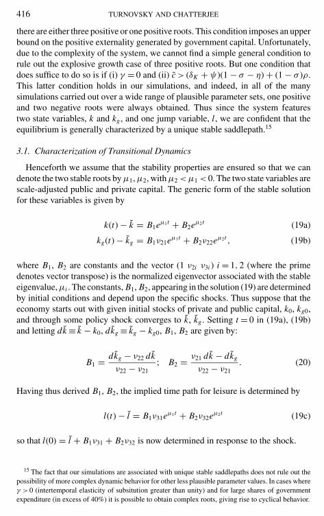
Henceforth we assume that the stability properties are ensured so that we candenote the two stable roots by µ1, µ2, with µ2 < µ1 < 0. The two state variables arescale-adjusted public and private capital. The generic form of the stable solutionfor these variables is given by
k(t) − k = B1eµ1t + B2eµ2t (19a)
kg(t) − kg = B1ν21eµ1t + B2ν22eµ2t , (19b)
where B1, B2 are constants and the vector (1 ν2i ν3i ) i = 1, 2 (where the primedenotes vector transpose) is the normalized eigenvector associated with the stableeigenvalue, µi . The constants, B1, B2, appearing in the solution (19) are determinedby initial conditions and depend upon the specific shocks. Thus suppose that theeconomy starts out with given initial stocks of private and public capital, k0, kg0,and through some policy shock converges to k, kg . Setting t = 0 in (19a), (19b)and letting dk ≡ k − k0, dkg ≡ kg − kg0, B1, B2 are given by:
B1 = dkg − ν22 dk
ν22 − ν21; B2 = ν21 dk − dkg
ν22 − ν21. (20)
Having thus derived B1, B2, the implied time path for leisure is determined by
l(t) − l = B1ν31eµ1t + B2ν32eµ2t (19c)
so that l(0) = l + B1ν31 + B2ν32 is now determined in response to the shock.
15 The fact that our simulations are associated with unique stable saddlepaths does not rule out thepossibility of more complex dynamic behavior for other less plausible parameter values. In cases whereγ > 0 (intertemporal elasticity of subsitution greater than unity) and for large shares of governmentexpenditure (in excess of 40%) it is possible to obtain complex roots, giving rise to cyclical behavior.

TO SPEND THE U.S. SURPLUS OR INCREASE THE DEFICIT 417
4. SOCIALLY OPTIMAL GOVERNMENT EXPENDITURE
One characteristic of our numerical results is that the benefits to increasing gov-ernment expenditure are limited. This is because there are socially optimal levelsof both types of expenditure. To see this it is useful to set out the steady-state equi-librium for the centrally planned economy in which the planner controls resourcesdirectly. The optimality conditions for such an economy consist of Eqs. (14), (16a),(16b), together with
c ≡ C
Y=
(1 − σ
θ
)(l
1 − l
)υ (15d′)
υσ
(y
k
)= δK + ρ + [1 − γ (1 + φ)]ψ + γ n (16c′)
υ = 1 + (q − 1)g + (φc − h) (21a)
υσy
k− δK = υ
η
q
y
kg− δG, (21b)
where υ denotes the shadow price of a marginal unit of output in terms of capitaland q denotes the shadow price of public capital in terms of private capital. Theseequations determine the steady-state solutions for c, y, l, k, kg, υ, q in terms of thearbitrarily set expenditure parameters g and h.
In contrast to the decentralized economy the after-tax prices relevant for themarginal rate of substitution condition in (15d′) and for the return to capital in(16c′) are replaced by the relative price of output in terms of consumption (capi-tal). Equation (21a) determines the relative price of output to capital. In the absenceof government expenditure, υ = 1. Otherwise, the social value of a unit of outputdeviates from the social value of capital due to the claims of government on outputand the value this has for the consumer. Specifically, with the size of governmentexpenditure being tied to aggregate output, an increase in output will divert re-sources away from private consumption, leaving 1 − g − h available to the agent.But offsetting this, public investment augments the stock of public capital, valuedat qg, and public consumption provides utility benefits equal to φc, making theoverall value of output to capital as described in (21a). The final equation equatesthe long-run net social returns to investments in the two types of capital.
Choosing the expenditure shares g and h optimally implies the socially optimalfractions of output devoted to government consumption and investment are
h = φc; q = 1, and hence υ = 1.
The marginal benefit of government consumption expenditure should equal itsresource cost, while the shadow values of the two types of capital should beequated. Substituting these conditions into (16b), (16c′), and (21b), the optimal
418 TURNOVSKY AND CHATTERJEE
share of output devoted to government production expenditure is
g = η[δG + ψ]
δG + ρ + [ [1 − γ (1 + φ)](1 − σ )1 − σ − η
+ γ]n
(22)
which provided γ < 0 implies g < η.16
5. CALIBRATING THE ECONOMY
We begin our numerical analysis of the alternative fiscal policies by calibratinga benchmark economy, using the following parameters representative of the USeconomy:
Production parameters α = 1, σ = 0.35, η = 0.20, n = 0.015, δK = 0.05,
δG = 0.05Preference parameters e = 1/(1 − γ ) = 0.4, i.e., γ = −1.5, ρ = 0.04,
θ = 1.75, φ = 0.3Fiscal parameters g = 0.08, h = 0.14, τw = 0.28, τk = 0.28
The elasticity on capital implies that approximately 35% of output accrues toprivate capital and the rest to labor, which grows at the annual rate of 1.5%.The elasticity η = 0.20 on public capital implies that public capital generates asignificant externality in production. The chosen value is substantially smallerthan the extreme value (0.39) suggested by Aschauer (1989) and lies within therange of the consensus estimates; see Gramlich (1994).
The preference parameters imply an intertemporal elasticity of substitutionin consumption of 0.4, consistent with empirical evidence; see, e.g., Ogaki andReinhart (1998).17 The elasticity of leisure θ = 1.75 accords with the value gen-erally chosen by real business cycle theorists and yields an equilibrium fractionof time devoted to leisure of about 0.7, consistent with the empirical evidence).The elasticity of 0.3 on government consumption implies that the optimal ratio ofgovernment consumption to private consumption is 0.3.
Our benchmark tax on wage income, τw = 0.28, reflects the average marginalpersonal income tax rate in the United States. Given the complex nature of capitalincome taxes, part of which may be taxed at a lower rate than wages, and part
16 This result contrasts with the optimal government expenditure in the Barro (1990) model, where,when government production expenditure impacts output as a flow, g = η. It is consistent with endoge-nous growth models, in which government production appears as a stock; see Futagami et al. (1993)and Turnovsky (1997). The replication of this by the decentralized economy requires that τk = τw = 0so that public expenditures are financed by appropriately set lump-sum taxes. However, this replicationis in general impossible here, given the other policy objective (government surplus reduction) beingsimultaneously imposed.
17 The empirical evidence on the intertemporal elasticity of substitution is quite varied, rangingbetween 0.1 (Hall, 1988) and 1 (Beaudry and van Wincoop, 1995).

TO SPEND THE U.S. SURPLUS OR INCREASE THE DEFICIT 419
at a higher rate, we have chosen the common rate τk = 0.28 as the benchmark.Government expenditure parameters have been chosen so that the total fraction ofnet national production devoted to government expenditure on goods and servicesequals 0.22, the historical average in the United States. The breakdown betweenh = 0.14 and g = 0.08 is arbitrary, but plausible. Government investment expen-diture is less than 0.08 and our choice of g = 0.08 is motivated by the fact that asubstantial fraction of government consumption expenditure, such as public healthservices, impacts as much on productivity as they do on utility. The annual (equal)depreciation rates δK = δG = 0.05 serve as a plausible benchmark case.
These parameters lead to the following plausible benchmark equilibrium, re-ported in Row 1 of Table I: fraction of time allocated to leisure, l = 0.71;consumption–output ratio is 0.64; the ratio of public to private capital is 0.58.18
The equilibrium levels of scale-adjusted private capital, public capital, and outputare 0.57, 0.33, and 0.52, respectively. Since these units are arbitrary (depending onα) they have all been normalized to unity. The corresponding quantities in the rowsbelow are all measured relative to the respective benchmark values of unity.19 Inaddition the steady-state growth rate, which by the nonscale nature of the economyis independent of policy, equals 2.17%.
The stable adjustment path for the benchmark economy is characterized bythe two stable eigenvalues (not reported), which are approximately −0.034 and−0.104. These imply that per capita output and capital converge at the asymptoticrate of approximately 2.7%, consistent with the accepted empirical evidence.20 Aninteresting feature of the model is that both stable roots are remarkably stable overthe fiscal exercises conducted.21
One of our primary concerns is the impact of the alternative policies on economicwelfare. This is measured by the optimized utility of the representative agent:
W ≡∫ ∞
0Z (t) dt =
∫ ∞
0
1
γ((C/N )lθ Hφ)γ e−ρt dt (23)
where Z (t) denotes instantaneous utility and C/N , l, H are evaluated along the
18 Estimates of time allocation studies suggest that households allocate somewhat less than one-third of their discretionary time to market activities (labor) and our equilibrium value l = 0.71 isgenerally consistent with that. Direct evidence on the ratio of public to private capital is sparse.Using the following relationships: (i) K = I − δK K , K G = G − δG KG . Assuming that on the balancedgrowth path that K/K = K G/KG and δK = δG implies the long-run relationship KG/K = kg/k =G/I . Taking G = 0.08, I = 0.14 yields the long-run ratio of public to private capital of around 0.57.
19 Thus, for example, in Row 2 the new steady-state stocks of private and public capital when h isincreased by 0.05 are 0.621.
20 These statements are based on the measure of the speed of convergence proposed by Eicher andTurnovsky (1999).
21 The unstable root is larger and more variable across policies. This implies that the speeds ofadjustments are fairly uniform across permanent fiscal changes, though they may vary across temporarypolicy changes; see Turnovsky (2001). The speed of convergence is also more sensitive to structuralchanges, such as changes in the productive elasticities.

420 TURNOVSKY AND CHATTERJEE
TAB
LE
I
Priv
ate
capi
tal
Publ
icca
pita
lO
utpu
tL
ong-
run
Shor
t-ru
nL
ong-
run
(rel
ativ
e(r
elat
ive
(rel
ativ
ego
vern
men
tw
elfa
rew
elfa
reτ k
τ wg
hl
ck g
/k
toba
se)
toba
se)
toba
se)
bala
nce
gain
sga
ins
A.L
ong-
Run
Eff
ects
ofFi
scal
Polic
ySh
ocks
Bas
eec
onom
y0.
280.
280.
080.
140.
706
0.64
30.
582
0.57
0(=
1)0.
332
(=1)
0.52
2(=
1)−0
.298
——
Incr
ease
inh
0.28
0.28
0.08
0.19
00.
689
0.59
30.
582
1.09
1.09
1.09
−0.0
50+1
.11%
+2.8
6%In
crea
sein
g0.
280.
280.
130
0.14
0.68
90.
593
0.94
31.
342.
181.
34−0
.050
−4.1
3%+3
.77%
Dec
reas
ein
τ k0.
140
0.28
0.08
0.14
0.69
70.
616
0.48
71.
431.
201.
20−0
.050
−4.3
1%+3
.49%
Dec
reas
ein
τ w0.
280.
203
0.08
0.14
0.68
50.
643
0.58
21.
111.
111.
00−0
.050
+0.3
2%+2
.51%
B.S
ome
Alte
rnat
ive
Polic
yM
ixes
and
Lon
g-R
unE
quili
briu
m
Bas
eec
onom
y0.
280.
280.
080.
140.
706
0.64
30.
582
0.57
0(=
1)0.
332
(=1)
0.52
2(=
1)−0
.298
——
Uni
form
incr
ease
0.28
0.28
0.10
50.
105
0.68
90.
593
0.76
31.
221.
601.
22−0
.050
−0.9
7%+3
.81%
ingo
vern
men
tex
pend
iture
sU
nifo
rmcu
tin
0.23
00.
230
0.08
0.14
0.68
90.
633
0.54
31.
221.
141.
14−0
.050
−1.3
4%+3
.00%
taxe
sO
ptim
algo
vern
men
t0.
284
0.28
0.10
90.
162
0.68
90.
592
0.79
81.
231.
691.
24−0
.050
−1.2
8%+3
.84%
expe
nditu
res
τ kad
just
sO
ptim
algo
vern
men
t0.
280.
282
0.10
90.
162
0.68
90.
592
0.79
81.
241.
691.
24−0
.050
−1.4
2%+3
.88%
expe
nditu
resτ w
adju
sts
Seco
nd-b
esto
ptim
al0.
160
0.34
80.
109
0.16
20.
701
0.56
90.
680
1.55
1.80
1.33
−0.0
50−5
.52%
+4.3
8%go
vern
men
tex
pend
iture
s

TO SPEND THE U.S. SURPLUS OR INCREASE THE DEFICIT 421
equilibrium path. The welfare gains reported are calculated as the percentagechange in the flow of base income necessary to maintain the level of welfareunchanged in response to the policy shock. The short-run impact is measured bythe changes in Z (t), while the long-run impact is summarized by the change in theoverall intertemporal index W .
The other key measure of economic performance, the measure of the intertem-poral fiscal balance has been defined previously in equation (8). For the chosenparameters tax revenues exceed government expenditures on goods and servicesby around 6% of current income.22 Evaluating (9) along the balanced growth pathand assuming without loss of generality that B0 = 0, we find that in the benchmarkcase, V = −0.298, a surplus nearly 30% measured in terms of current income. Inall cases, the fiscal policies we consider involve reducing the surplus from its ini-tial value of V = −0.298 to V = −0.05. However, the results are insensitive to thearbitrarily chosen level of B0 and thus V ; what is relevant is the reduction in V .23
6. REDUCING THE SURPLUS (INCREASING THE DEFICIT)
Rows 2–5 in Table I-A describe the four basic policy changes from the bench-mark economy, with the corresponding dynamic transition paths being illustratedin Figs. 1–4. One striking pattern throughout all simulations is that the labor sup-ply responds almost completely upon impact to an unanticipated permanent shock.After the initial jump, the transitional path for labor supply is virtually flat. Thereason for this is that for plausible parameter values the elements a12, a13 in thetransitional matrix in (18) are both small relative to a11 > 0; there is little feedbackfrom the changing stocks of capital to labor supply. In other words, the dynamicsof labor can be approximated by the unstable first order system
dl(t)/dt = a11(l(t) − l)
which for bounded behavior essentially requires that l jump to steady state.
6.1. Increase in Government Consumption Expenditure
One way of reducing the surplus from −0.298 to −0.05 is to increase govern-ment consumption expenditure h by 0.05 percentage points from 0.14 to 0.19.This increases long-run private capital, public capital, and output proportionatelyby 9%, while crowding out the long-run private consumption–output ratio by 0.05percentage points, with a corresponding reduction in leisure by 0.02. The lowerprivate consumption and higher labor supply reduce welfare, while the higher
22 This accords approximately with recent data on the surplus of government account on goods andservices.
23 The reduction in V we consider is equivalent to 25% of current income, an amount something inexcess of 2 trillion dollars.

422 TURNOVSKY AND CHATTERJEE
government consumption is welfare increasing. On balance, the latter effect dom-inates and short-run welfare increases by a little over 1%. The higher employmentincreases the productivity of capital, stimulating its accumulation and the growth ofoutput over time. Thus, despite the reduction in the long-run consumption–outputratio the accumulation of capital and growth of output over time implies that thefall in absolute consumption is small so that overall welfare rises by 2.86% relativeto the benchmark.
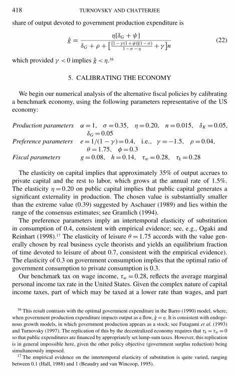
The dynamics of this shock are illustrated in the four panels of Fig. 1. Theimmediate effect of the lump-sum tax-financed increase in expenditure is to reducethe private agent’s wealth, inducing him or her to supply more labor, thereby raisingthe marginal productivity of both types of capital and raising output.
The phase diagram Fig. 1a indicates that the two capital stocks accumulateapproximately proportionately. This is also reflected in their growth rates (Fig. 1b),which both jump initially to around 2.5% and track one another closely as theyboth gradually decline to their steady-state rates of around 2.2%, as both types ofcapital accumulate and their respective rates of return decline. With the labor supplyremaining virtually fixed after the initial jump, the growth rate of output is belowthat of either form of capital during the transition. In Fig. 1c the implied adjustmentpaths of output, consumption, and employment are illustrated relative to theirrespective benchmark economies. As noted, upon impact, the initial expenditureincrease raises instantaneous welfare by over 1% and this grows uniformly withthe growth in the capital stocks and output to an asymptotic improvement relativeto the benchmark, of over 5%, the present value of which is 2.86%. Finally, theexpenditure increase drastically reduces the current government deficit relativeto the benchmark economy, which then rises modestly throughout the transition,reflecting the corresponding rise in the growth of output.24
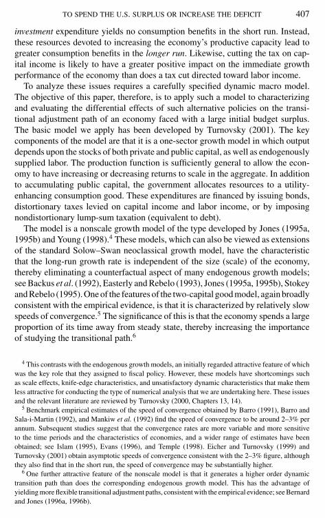
6.2. Increase in Government Investment Expenditure
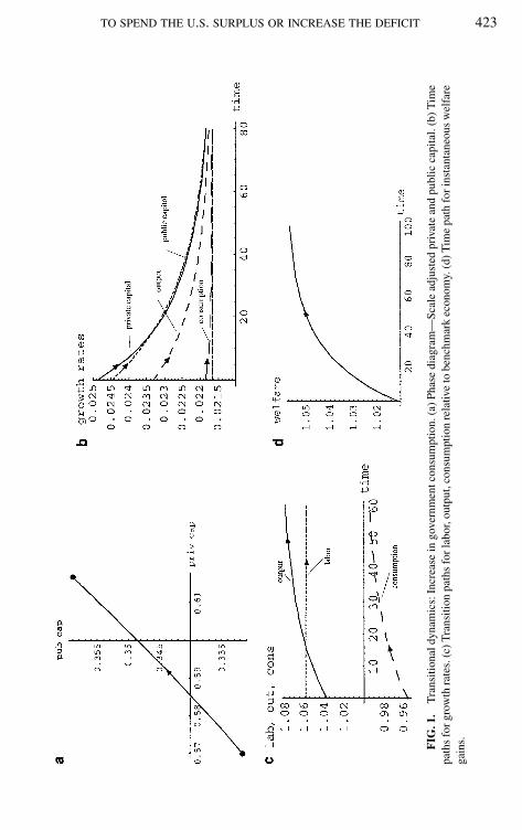
Increasing the rate of government expenditure g by 0.05 from 0.08 to 0.13 alsowill reduce the surplus from −0.298 to −0.05.25 But it is associated with markedlydifferent equilibrium responses and therefore long-run capital structure. Long-runprivate capital and output both increase by 34%, and public capital increases by118%, raising the ratio of public to private capital from 0.58 to 0.94. The effects onemployment and the consumption–output ratio are precisely as for h, as noted inTable I. The reduction in initial consumption and leisure, illustrated in Fig. 2c, withno immediate public expenditure benefits, leads to an initial reduction in welfareof 4.13% (Fig. 2d), although the long-run increase in productive capacity raisesoverall welfare.
24 These paths are almost all identical for the different modes of reducing the surplus and are notillustrated.
25 Actually, the amounts of the government expenditures consistent with the same reduction in theintertemporal surplus differ slightly in the two cases. Because of the larger increases in Y (t) over time,the increase in g is only 0.0496, rather than 0.05. We have computed the policies and the impliedtransitional dynamics using the more accurate numbers.
TO SPEND THE U.S. SURPLUS OR INCREASE THE DEFICIT 423
FIG
.1.
Tra
nsiti
onal
dyna
mic
s:In
crea
sein
gove
rnm
entc
onsu
mpt
ion.
(a)
Phas
edi
agra
m—
Scal
ead
just
edpr
ivat
ean
dpu
blic
capi
tal.
(b)
Tim
epa
ths
for
grow
thra
tes.
(c)
Tra
nsiti
onpa
ths
for
labo
r,ou
tput
,con
sum
ptio
nre
lativ
eto
benc
hmar
kec
onom
y.(d
)T
ime
path
for
inst
anta
neou
sw
elfa
rega
ins.
424 TURNOVSKY AND CHATTERJEE
FIG
.2.
Tra
nsiti
onal
dyna
mic
s:In
crea
sein
gove
rnm
enti
nves
tmen
t.(a
)Ph
ase
diag
ram
—sc
ale
adju
sted
priv
ate
and
publ
icca
pita
l.(b
)T
ime
path
sfo
rgr
owth
rate
s.(c
)T
rans
ition
path
sfo
rla
bor,
outp
ut,c
onsu
mpt
ion
rela
tive
tobe
nchm
ark
econ
omy.
(d)
Tim
epa
thfo
rin
stan
tane
ous
wel
fare
gain
s.

TO SPEND THE U.S. SURPLUS OR INCREASE THE DEFICIT 425
The dynamic adjustments paths followed by the two capital stocks are in sharpcontrast both to one another and to the adjustment that occurs in response to anequivalent increase in government consumption. The initial claim on capital bythe government crowds out private investment, so that the growth rate of privatecapital is reduced below the growth rate of population; the scale-adjusted stock ofprivate capital therefore initially declines. By contrast, the direct investment raisesthe initial growth rate of public capital to over 6% (see Fig. 2b), although thisthen declines steadily over time as the increase in its stock reduces the return tofurther public investment. As the new public capital is put in place, its productivityraises the return to private capital, thereby stimulating its rate of accumulation andits growth rate. Over time, as the more public capital is in place and its growthrate declines, this effect is mitigated and the growth rate of private capital, afterinitially rising, begins to fall to its constant steady-state rate. Thus, whereas thegrowth rates of the two forms of capital track one another closely in response toan increase in h, they diverge markedly during the transition in the present case.
As capital is accumulated and output and consumption grow, so does welfare,and asymptotically the instantaneous welfare rises 25% above the base level. Thepresent value of this increase, after allowing for the initial loss, is around 4.13%.
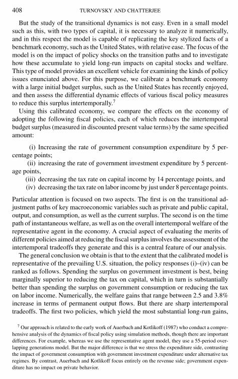
6.3. Decrease in Tax on Capital
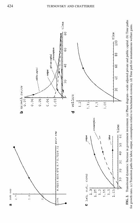
A third way to reduce the surplus to −0.05 is to lower the tax on capital incomefrom 0.28 to 0.140. This also has a dramatic long-run effect, increasing privatecapital by about 43% and public capital and output by around 20%. The dynamicsare illustrated in Fig. 3. The reduced tax on capital increases the return to laborleading to an initial substitution toward more labor and less consumption. Initiallywelfare falls by 4.31% (Fig. 3d). Upon impact, the lower tax raises the growthrate on private capital to around 5%, so that the scale-adjusted per capita stock,k, begins to increase rapidly. The increase in labor and the increase in privatecapital increases the growth rate of output, and the growth rate of public capitalbegins to rise as well, so that k and kg follow the increasing paths in Fig. 3a.With the incentive applying directly to private capital, k increases relative to kg
during the initial stages. But as private capital increases in relative abundanceits productivity declines, inducing less investment in private capital and therebyretarding its growth rate. This in turn reduces the productivity of public capital, theincreasing growth rate of which is reversed after 15 periods. The steady increase inrelative consumption over time implies that after the initial decrease, instantaneouswelfare increases steadily relative to the benchmark, increasing asymptotically byabout 12.5%. The present value of this increase is equivalent to a 3.49% increase inincome. Thus we see that reducing the surplus by reducing the tax on capital incomeis significantly superior to spending the surplus on a government consumption goodand is nearly as good as spending the surplus on a government investment good.And like the latter it involves a sharp intertemporal tradeoff in benefits. In bothcases significant short-run welfare losses must be incurred in order to obtain largelong-run welfare gains resulting from the stimulus to investment in both cases.
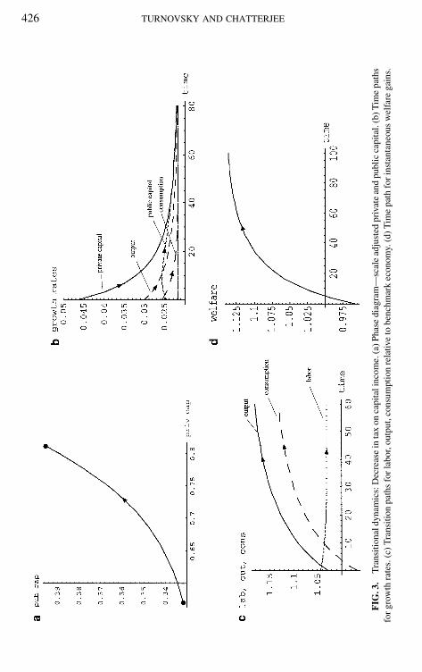
426 TURNOVSKY AND CHATTERJEE
FIG
.3.
Tra
nsiti
onal
dyna
mic
s:D
ecre
ase
inta
xon
capi
tali
ncom
e.(a
)Pha
sedi
agra
m—
scal
ead
just
edpr
ivat
ean
dpu
blic
capi
tal.
(b)T
ime
path
sfo
rgr
owth
rate
s.(c
)T
rans
ition
path
sfo
rla
bor,
outp
ut,c
onsu
mpt
ion
rela
tive
tobe
nchm
ark
econ
omy.
(d)
Tim
epa
thfo
rin
stan
tane
ous
wel
fare
gain
s.
TO SPEND THE U.S. SURPLUS OR INCREASE THE DEFICIT 427
FIG
.4.
Tra
nsiti
onal
dyna
mic
s:D
ecre
ase
inta
xon
labo
rin
com
e.(a
)Ph
ase
diag
ram
—sc
ale
adju
sted
priv
ate
and
publ
icca
pita
l.(b
)T
ime
path
sfo
rgr
owth
rate
s.(c
)T
rans
ition
path
sfo
rla
bor,
outp
ut,c
onsu
mpt
ion
rela
tive
tobe
nchm
ark
econ
omy.
(d)
Tim
epa
thfo
rin
stan
tane
ous
wel
fare
gain
s.
428 TURNOVSKY AND CHATTERJEE
6.4. Decrease in Tax on Wage Income
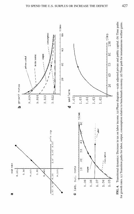
Finally, the government may reduce the surplus by reducing the tax on laborincome to 0.203. The effects of this are much closer to those of an increase ingovernment expenditure on consumption. Private capital, public capital, and outputall increase proportionately by around 11% and labor supply is reduced by 0.02. Asin the other shocks, the increase in employment occurs virtually instantaneously,reducing short-run welfare. On the other hand, the reduction in the tax on laborincome stimulates initial consumption by around 5% and this is welfare improving.Overall, the latter effect dominates and welfare improves slightly in the short runby around 0.32%. The increase in employment enhances the productivity of bothprivate and public capital which are accumulated over time. As in the case of anincrease in government consumption expenditure, which does not impact on eitherform of capital directly, the lower tax on labor income stimulates the accumulationof both types of capital approximately equally, so that their respective growth ratestrack one another closely. The accumulation of capital and the output over timeraises consumption and intertemporal welfare increases by around 2.5%. Thus, atleast for the model as parameterized, reducing the tax on labor income is dominatedby the other policies we have considered.
6.5. Other Policy Mixes
The four policies considered in Table I-A describe the basic options and wenow address some alternatives summarized in Table I-B. First, we see that increas-ing government expenditure uniformly on the two types of good by 0.025 eachis marginally superior to increasing expenditure on the productive input alone.This is because there are in fact optimal degrees of expenditure on both types ofgovernment goods g = 0.109, h = 0.162, respectively. Increasing g from its initialvalue of 0.08 to 0.13 takes it too far beyond the optimum. The uniform increasetakes g to 0.105 and h to 0.165, both close to their respective optima. By contrast,a uniform cut in the tax rate to 0.23 is significantly inferior to targeting the capitalincome tax alone.
The final three policy shocks involve setting the two forms of government expen-diture at their respective optimal values. This involves increasing total governmentexpenditure by 0.051, requiring a slight adjustment in the tax rates in order to main-tain the long-run surplus at its target level of −0.05. In the first case this can beaccomplished by raising the tax on capital income from 0.28 to 0.284; in the secondcase it is done by raising the tax on labor income slightly from 0.28 to 0.282. Ofthese two options, the latter is marginally superior.
However, greater gains can be obtained by increasing the tax on labor andreducing it correspondingly on capital. Indeed the optimal fiscal mix consistentwith maintaining the surplus at its target level of −0.05 is to set expenditures attheir respective optimal values g = 0.109, h = 0.162, reduce the tax on capital to0.160, and raise the tax on labor income to 0.348. While this will lead to substantialshort-run welfare losses while consumption is foregone and capital is accumulated,
TO SPEND THE U.S. SURPLUS OR INCREASE THE DEFICIT 429
this will be more than offset by long-run welfare gains, the present value of whichis around 4.4%. These results suggest that further welfare gains can be attained bycombining the reduction of the surplus with some revision of the tax structure.
7. SOME SENSITIVITY ANALYSIS
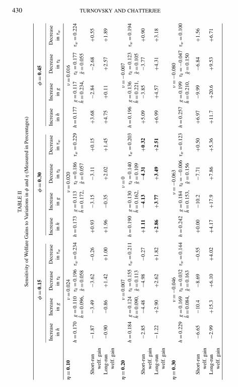
The sensitivity of utility to government consumption, φ, and the productivityof public capital, η, are two key parameters. While the values we have chosen areplausible for the United States, the empirical evidence on them is sparse and in somecases far-ranging. Table II therefore summarizes the welfare effects obtained forthe combination of cases over the ranges φ = 0.15, 0.30, 0.45 and η = 0.10, 0.20,0.30. These we identify with low, medium, and high direct impacts of governmentexpenditure, respectively. Varying the parameters in this way also aids in ourappreciation of the importance of the levels of government expenditure relative totheir respective optima.
In studying Table II we should point out that changes in the structural parametersφ and η will generate differences in the initial government surplus V. To preservecomparability we shall normalize everything so that all changes begin from thesame initial government surplus V = −0.298. This is done by simply introducing atransfer term ν which has no effect on any other aspect of the equilibrium. Thus inall cases, our experiments begin with the same initial tax and expenditure structure,g = 0.08, h = 0.13, τk = τw = 0.28, with the corresponding surplus V = −0.298and reducing V to −0.050, as in Table I. The cell in bold letters corresponds tothe base parameter set assumed in Table I. The quantities h = 0.19 etc. in thebox describes the increase in h consistent with reducing the surplus to −0.05, andh = 0.162 describes the optimum. All other boxes are similar, but the main point toobserve is that the magnitude of the elasticity parameters φ and η has an importantbearing on the magnitudes of the tax and expenditure changes that are consistentwith reducing the surplus by the (common) required amount.
From Table II we can detect the following patterns:
1. Decreasing the tax rate on labor income always yields long-run (intertem-poral) benefits which, not surprisingly, increase with the importance of governmentconsumption in utility, φ. Less obviously, they also increase with the productivityof public capital, η, and indeed are more sensitive to increases in the latter. Thisis because the decrease in τw stimulates employment, which interacts with bothtypes of capital in production. The more productive public capital, the more outputincreases, ultimately generating greater consumption benefits.
2. The short-run welfare effects of decreasing the tax rate on labor incomedepend upon φ and will be mildly adverse if φ is small (0.15). This is because thepositive short-run consumption benefits stemming from the lower tax rate are nowdominated by the adverse employment effects.
3. Decreasing the tax rate on capital income always has adverse short-runeffects on welfare but positive long-run benefits. This is because by directing
430 TURNOVSKY AND CHATTERJEE
TAB
LE
IISe
nsiti
vity
ofW
elfa
reG
ains
toV
aria
tions
inφ
and
η(M
easu
red
inPe
rcen
tage
s)
φ=
0.15
φ=
0.30
φ=
0.45
Incr
ease
Incr
ease
Dec
reas
eD
ecre
ase
Incr
ease
Incr
ease
Dec
reas
eD
ecre
ase
Incr
ease
Incr
ease
Dec
reas
eD
ecre
ase
inh
ing
inτ k
inτ w
inh
ing
inτ k
inτ w
inh
ing
inτ k
inτ w
η=
0.10
ν=
0.02
4ν
=0.
020
ν=
0.01
6h
=0.
170
g=
0.11
0τ k
=0.
196
τ w=
0.23
4h
=0.
173
g=
0.11
3τ k
=0.
186
τ w=
0.22
9h
=0.
177
g=
0.11
7τ k
=0.
177
τ w=
0.22
4h
=0.
096,
g=
0.05
8h
=0.
172,
g=
0.05
7h
=0.
234,
g=
0.05
5
Shor
t-ru
n−1
.87
−3.4
9−3
.62
−0.2
6+0
.93
−3.1
5−3
.11
+0.1
5+3
.68
−2.8
4−2
.68
+0.5
5w
elf.
gain
Lon
g-ru
n−0
.90
−0.8
6+1
.42
+1.0
0+1
.96
−0.3
5+2
.02
+1.4
5+4
.75
+0.1
1+2
.57
+1.8
9w
elf.
gain
η=
0.20
ν=
0.00
7ν
=0
ν=
−0.0
07h
=0.
184
g=
0.12
4τ k
=0.
155
τ w=
0.21
1h
=0.
190
g=
0.13
0τ k
=0.
140
τ w=
0.20
3h
=0.
196
g=
0.13
6τ k
=0.
123
τ w=
0.19
4h
=0.
090,
g=
0.11
3h
=0.
162,
g=
0.10
9h
=0.
221,
g=
0.10
5Sh
ort-
run
−2.8
5−4
.48
−4.9
8−0
.27
+1.1
1−4
.13
−4.3
1+0
.32
+5.0
9−3
.85
−3.7
7+0
.90
wel
f.ga
inL
ong-
run
−1.2
2+2
.90
+2.6
2+1
.82
+2.8
6+3
.77
+3.4
9+2
.51
+6.9
9+4
.57
+4.3
1+3
.18
wel
f.ga
in
η=
0.30
ν=
−0.0
46ν
=−0
.063
ν=
−0.0
80h
=0.
229
g=
0.16
9τ k
=0.
032
τ w=
0.14
4h
=0.
242
g=
0.18
4τ k
=−0
.006
τ w=
0.12
3h
=0.
257
g=
0.19
9τ k
=−0
.047
τ w=
0.10
0h
=0.
084,
g=
0.16
3h
=0.
153,
g=
0.15
6h
=0.
210,
g=
0.15
0
Shor
t-ru
n−6
.65
−10.
4−8
.69
−0.5
5+0
.00
−10.
2−7
.71
+0.5
0+6
.97
−9.9
9−6
.84
+1.5
6w
elf.
gain
Lon
g-ru
n−2
.99
+15.
3+6
.10
+4.0
2+4
.17
+17.
9+7
.86
+5.3
6+1
1.7
+20.
6+9
.53
+6.7
1w
elf.
gain

TO SPEND THE U.S. SURPLUS OR INCREASE THE DEFICIT 431
resources toward private investment, consumption and leisure are both reduced inthe short run. Over time, the increased capital stock leads to more output, moreconsumption, and positive welfare effects. The intertemporal tradeoff in benefitsincrease sharply with the productivity of public capital. A larger η increases thereturns to sacrificing consumption in the short run for greater future consumptionbenefits.
4. An increase in government consumption expenditure will produce posi-tive short-run and long-run benefits provided φ is sufficiently large. However, ifφ is small increasing h is welfare-deteriorating. This is because the initial bench-mark value of h = 0.14, from which the increase is occurring, is greater than thesocially optimal level, h. The increase in utility obtained from more governmentconsumption is dominated by the losses incurred from the crowding out of privateconsumption and decline in leisure. Both the short-run and long-run benefits fromgovernment consumption increase with φ. In contrast, the short-run and long-runbenefits from government consumption increase with the productivity of publiccapital η as long as the utility of government consumption is sufficiently large.However, if the latter are small, an increase in the productivity of governmentproduction simply exacerbates the losses stemming from increased governmentconsumption.
5. An increase in government investment expenditure is always associatedwith short-run welfare losses, as resources are diverted away from consumption.In general, the increase in government capital will generate positive long-run wel-fare gains, unless the direct impacts of public capital and public consumptionare both small. Thus, for example, if φ = 0.15, η = 0.10, the initial rates of gov-ernment expenditure (g = 0.08, h = 0.14) exceed their respective social optima(g = 0.058, h = 0.096) so that any further government investment is undesirable.Both the short-run welfare losses and the long-run gains resulting from an increasein government investment increase with its productivity η. That is, the more pro-ductive government sharpens the intertemporal tradeoff in benefits from furtherinvestment.
The relative desirability of the four alternative modes of spending the surplusis sensitive to the direct impacts of the two forms of government spending. In thisrespect the following rankings can be observed.
1. For the calibrated U.S. economy increasing government investment isbest, followed by reducing the tax on capital, increasing government consumptionexpenditure, and reducing the tax on labor income.
2. Decreasing the tax on capital is always superior to decreasing the tax onlabor income.
3. If the benefits of both forms of government expenditure are low (φ = 0.15,η = 0.10) reducing the tax rate on capital is best, while increasing governmentconsumption expenditure is worst. If the benefits of government consumptionare high and government investment remain low (φ = 0.45, η = 0.10) increasing
432 TURNOVSKY AND CHATTERJEE
government consumption becomes the best policy and government investment theworst. If the benefits of government investment are high and government consump-tion remain low (φ = 0.15, η = 0.30) these rankings are reversed. If the benefits ofboth forms of government expenditure are high (φ = 0.45, η = 0.30) both forms ofgovernment expenditure dominate both forms of tax cuts, with investment beingthe preferred policy.
8. CONCLUSIONS AND CAVEATS
How to spend the projected budget surplus has generated a lively policy debate.This paper has provided a numerical analysis of the likely benefits from adoptingdifferent policy options in a model calibrated to approximate the U.S. economy.Our results suggest that insofar as the U.S. economy is concerned, to invest thegovernment surplus productively will yield the greatest long-run welfare gains ofaround 3.8%. Decreasing the tax on capital income is only marginally inferior,yielding welfare gains of around 3.5%. Both of these options clearly dominate in-creasing government consumption expenditure (welfare gains 2.9%) or decreasingthe tax on labor income (welfare gains 2.5%).
The two superior policy options—increasing the rate of government investmentor reducing the tax on capital income—have the characteristic that they impingedirectly on the rates of accumulation of one of the types of capital. By shiftingresources directly toward the accumulation of capital and away from consumptionthey induce significant short-run welfare losses that are more than compensatedby large long-run welfare gains. They are therefore both characterized by sharpintertemporal tradeoffs in welfare. But at the same time they will ultimately leadto very different economic structures, at least insofar as the mix between publicand private capital is concerned. By contrast, the two inferior options impinge onlyindirectly on capital accumulation. Accordingly they are associated with mildlyuniform increases in welfare through time. In addition, they have no long-runimpact on the long-run mix between public and private capital.
Either form of government spending is associated with a socially optimal expen-diture level. Thus a crucial determinant of the benefits of reducing the governmentsurplus through spending is the size of government spending relative to the so-cial optimum. For the calibrated economy devoting the entire surplus to one formof expenditure is not optimal, as it increases that form of expenditure beyondits social optimum. Indeed, we find that the second-best optimum is to increaseboth forms of government expenditure to their respective social optima, while atthe same time restructuring taxes by reducing the tax on capital and raising thetax on wage income, subject to the targeted reduction in the budget surplus. Inother circumstances, increasing either form of government expenditure may bewelfare-deteriorating.
While we find our numerical results to be plausible, we should not lose sight ofthe fact that they are derived from a stylized economic model that abstracts from

TO SPEND THE U.S. SURPLUS OR INCREASE THE DEFICIT 433
many important theoretical and practical aspects. The policy implications thereforeneed be interpreted with some caution, and considered within the broader economicand political framework within which the government operates. It is thereforeuseful to acknowledge some of the limitations of our analysis.
First, the investment option available to the government has been restricted topublic (physical) capital. It is the interaction of public capital with private capitalthat is the key source of economic growth, and the more productive is governmentcapital, the higher the long-run growth rate will be. In addition, public capital hasbeen assumed to be a pure public good, free of congestion. This assumption isclearly a polar one, since almost all public services are subject to some degreeof congestion. Eicher and Turnovsky (2000) develop a simple nonscale growthmodel in which productive public expenditure, introduced as flow (as in Barro1990), is subject to two types of congestion. They discuss the effects of bothtypes of congestion on the long-run growth rate, the speed of convergence, and theequilibrium capital stock. Although they do not address the issue, their model alsoimplies that congestion reduces the productivity of the public input. The reductionin the productivity parameter, η, briefly considered in Section 7, can be viewed asa partial attempt to take account of congestion in this model. But clearly, this is animportant issue and is a dimension in which the present model of public capitalcould be fruitfully extended.
Second, the model excludes human capital and knowledge-based capital, a keysource of growth in the class of endogenous growth models pioneered by Lucas(1988). Indeed, the choice between investing in human capital and physical capitalis an important policy decision and needs to be addressed in an integrated modelthat includes both types of capital. It seems plausible to conjecture that taxes onlabor income will have a greater impact on transitional growth rates and economicperformance in an economy in which agents are choosing between accumulatinghuman as well as and physical capital. But in order to be more precise as to the extentthat this might be so, one needs to distinguish between the decision to supply rawlabor and the decision to acquire skills through the accumulation of human capital.
Third, there are several other sources of growth that are excluded from thismodel. These include the accumulation of knowledge, the development of newtechnology, reduced regulation, the reform of financial systems, and so on. Thereare also the political aspects, and these too need to be taken into account. In part asa political compromise most of the tax cuts proposed by the Bush administrationare being phased in over a number of years. A consideration of the timing aspectsof these policies therefore merits further investigation.
More important, political decisions are driven by short-run considerations. Thusfor example, whereas increasing government investment may yield the largest long-run benefits, the fact that it is also associated with large short-run losses may inhibitpoliticians from adopting the preferred long-run policy. Indeed, being a long-runequilibrium model that abstracts from short-run rigidities it does not focus on thetypes of short-run issues, such as job creation, that tend to attract the attention ofpoliticians.

434 TURNOVSKY AND CHATTERJEE
One final matter concerns distributional aspects, an issue having several dimen-sions. Since the basic framework we have employed is a Ramsey-type model withan infinitely lived agent, it is characterized by Ricardian equivalence. The initialstock of government debt, B0, does not matter per se. The real effects we havebeen discussing arise from the impact of the real fiscal changes introduced—theexpenditure and tax rates—and precisely the same results would obtain if budget-balance through issuing additional debt was maintained at all times. Thus theRamsey model has no implications for intergenerational distribution issues. Yetthese issues are an important part of the debate, but to study them one would needto adopt an alternative framework such as a finite-lived overlapping generationsmodel.
The relationship between income distribution (inequality) and growth is becom-ing topical, with no definitive conclusions at this time concerning the causality orrelationship between them. Here one can distinguish between functional incomedistribution (the distribution between factors) and personal income distribution.The present framework cannot address either aspect satisfactorily. Being basedon a Cobb–Douglas production function, (pre-tax) income shares, one measureof functional income distribution, are constant through time, being determined bytheir respective exponents in the production function. A more general productionfunction is therefore required in order to analyze this aspect in a more profoundway. To analyze personal income distribution, one needs to extend the model toinclude heterogeneous agents, indexed say by their initial endowments of privateor human capital. Both of these extensions are feasible and are directions in whichthe present model should be developed in order to gain a complete understandingof the consequences of alternative fiscal policies.
REFERENCES
Aschauer, D. A. (1989). Is public expenditure productive? J. Monet. Econ. 23, 177–200.
Auerbach, A. J., and Kotlikoff, L. J. (1987). “Dynamic Fiscal Policy,” Cambridge University Press,Cambridge UK.
Backus, D., Kehoe, P., and Kehoe, T. (1992). In search of scale effects in trade and growth. J. Econ.Theory 58, 377–409.
Barro, R. J. (1990). Government spending in a simple model of endogenous growth. J. Polit. Econ. 98,S103–S125.
Barro, R. J. (1991). Economic growth in a cross-section of countries. Quart. J. Econ. 106, 407–443.
Barro, R. J., and Sala-i-Martin, X. (1992). Convergence. J. Polit. Econ. 100, 223–251.
Beaudry, P., and van Wincoop, E. (1995). The intertemporal elasticity of substitution: An explorationusing U.S. panel of state data. Economica 63, 495–512.
Bernard, A. B., and Jones, C. I. (1996a). Technology and convergence. Econ. J. 106, 1037–1044.
Bernard, A. B., and Jones, C. I. (1996b). Comparing apples and oranges: Productivity consequencesand measurement across industries and countries. Amer. Econ. Rev. 86, 1216–1238.
Bruce, N., and Turnovsky, S. J. (1999). Budget balance, welfare, and the growth rate: Dynamic scoringof the long-run government budget. J. Money, Credit, Banking 31, 162–186.

TO SPEND THE U.S. SURPLUS OR INCREASE THE DEFICIT 435
Easterly, W., and Rebelo, S. (1993). Fiscal policy and growth: An empirical investigation. J. Monet.Econ. 32, 417–458.
Eicher, T. S., and Turnovsky, S. J. (1999). Convergence speeds and transition dynamics in non-scalegrowth models. J. Econ. Growth 4, 413–428.
Eicher, T. S., and Turnovsky, S. J. (2000). Scale, congestion, and growth. Economica 67, 325–346.
Evans, P. (1997). How fast do countries converge? Rev. Econ. Statist. 79, 219–225.
Futagami, K., Morita, Y., and Shibata, A. (1993). Dynamic analysis of an endogenous growth modelwith public capital. Scand. J. Econ. 95, 607–625.
Gramlich, E. M. (1994). Infrastructure investment: A review essay. J. Econ. Lit. 32, 1176–1196.
Hall, R. E. (1988). Intertemporal substitution in consumption, J. Polit. Econ. 96, 339–357.
Islam, N. (1995). Growth empirics: A panel data approach, Quart. J. Econ. 110, 1127–1170.
Jones, C. I. (1995a). R&D based models of economic growth. J. Polit. Econ. 103, 759–784.
Jones, C. I. (1995b). Time-series tests of endogenous growth models. Quart. J. Econ. 110, 495–525.
Lucas, R. E. (1988). On the mechanics of economic development, J. Monet. Econ. 22, 3–42.
Mankiw, N. G., Romer, D., and Weil, D. (1992). A contribution to the empirics of economic growth.Quart. J. Econ. 107, 407–438.
Mankiw, N. G., Rotemberg, J., and Summers, L. H. (1985). Intertemporal substitution in macroeco-nomics. Quart. J. Econ. 100, 225–251.
Ogaki, M., and Reinhart, C. M. (1998). Measuring intertemporal substitution: the role of durable goods.J. Polit. Econ. 106, 1078–1098.
Stokey, N. L., and Rebelo, S. (1995). Growth effects of flat-rate taxes. J. Polit. Econ. 103, 519–550.
Temple, J. R. W. (1998). Robustness test of the augmented Solow model. J. Appl. Econ. 13, 361–375.
Turnovsky, S. J. (1997). Public and private capital in an endogenously growing economy. Macroecon.Dynam. 1, 615–639.
Turnovsky, S. J. (2000). “Methods of Macroeconomic Dynamics.” 2nd ed., MIT Press, Cambridge,MA.
Turnovsky, S. J. (2001). The transitional dynamics of fiscal policy: Long-run capital accumulation andgrowth. J. Money, Credit, Banking, forthcoming.
Young, A. (1998). Growth without scale effects. J. Polit. Econ. 106, 41–63.