AD-A156 939 MODELS TO PREDICT THE PERFORMANCE OF AXIAL FLOW CRSON /DIOXIDE ABSORPTIVE CANISTERS(U) NRAVAL POSTORADUATESCHOOL MONTEREY CH Y E YARBOROUGH MAlR 85

UNCLSSIFIED F/G 12/ NL

12,8 12.5

I1.8I1.25 1.4SllII Illl I.

MICROCOPY RESOLUI N - .

NATION", ( ;I N

Ln NAVAL POSTGRADUATE SCHOOL

Monterey, California

<p

JUL 1 5 1985 j

GTHESIS

MODELS TO PREDICT THE PERFORMANCE OF AXIALFLOW CARBON DIOXIDE ABSORPTIVE CANISTERS

by

Joseph Earl Yarborough, Jr.

C...) March 1985

LA.-

Thesis Advisor: Charles W. Hutchins Jr.

-- Approved for public release; distribution unlimited.

85 06 24 022l

. . . .

UNCLASSIFIEDSECURITY CLASSIFICATION OF THIS PAGE ("he, Date MEntered)

REPORT DOCUMENTATION PAGE READ INSTRUCTIONSR . PBEFORE COMPLETING FORM

FI. REPORT NUMBER 2.~j~ GVAC SIS t,~ g# LOG NUMBER

4. TITLE (and Subtitle) S-. TYPE OF REPORkA PERIOD COVERED

Models to Predict the Performance of Master's ThesisAxial Flow Carbon Dioxide Absorptive March 1985Canisters 6. PERFORMING ORG. REPORT NUMBER

7. AUTHOR(@) I. CONTRACT OR GRANT NUMBER(s)

Joseph Earl Yarborough, Jr.

9. PERFORMING ORGANIZATION NAME AND ADDRESS 10. PROGRAM ELEMENT. PROJECT, TASK

Naval Postgraduate School AREA & WORK UNIT NUMBERS

Monterey, California 93943

II CONTROLLING OFFICE NAME AND ADDRESS 12. REPORT DATE

Naval Postgraduate School March 1985Monterey, California 93943 13. NUMBER OF PAGES

8014. MONITORING AGENCY NAME & ADDRESS(If different from Controlling Office) IS. SECURITY CLASS. (of this report)

UNCLASSIFIED

1S. DECLASSIFICATION, DOWNGRADINGSCHEDULE

16. DISTRIBUTION STATEMENT (of this Report)

Approved for public release; distribution unlimited.

17. DISTRIBUTION STATEMENT (ol the obetroct entered In Block 20, if different from Report)

I I. SUPPLEMENTARY NOTES

" 19. KEY WORDS (Continue on reverse elde It neceeary end Identify by block number)

Carbon Dioxide, Absorption, Linear Regression, Data Analysis,Cross Validation

20, ABSTRACT (Continue on reverse side It neceee y and Identify by block number)

Models were developed using the techniques of multiple

regression to predict the time at which the carbon dioxide

concent.-,ion in a gas stream that exits a canister, exceeds

the physiological limit for human respiration. Additional

DD J . 1473 EDITION OF 1 NOV 65 IS OBSOLETEUNCLASSIFIED0102- LF- 014. 6601 1 SECURITY CLASSIFICATION OF THIS PAGE (When Det Ent-ered)

UNCLASSIFIEDSECURITY CLASSIFICATION Of THIS PAGE ( Daui 00 EMIS640

#20 - Abstract - (CONTINUED)

models were developed to predict canister efficiency

as a function of various geometric and environmental

parameters. Simple cross validation was performed in

both cases to provide a measure of model applicability.

'.y

S /m

S N 0102:-LF-014.6601

2 UNCLASSIFIEDSECUNITY CLASSIFICATION OF THIS PAE[(Whfl Dl0 t *trod

Approved for public release; distribution unlimited.

Models to Predict the Performance of Axial

Flow Carbon Dioxide Absorptive Canisters

by

Joseph Earl Yarborough, Jr.Lieutenant Commander, United States NavyB.S., University of South Carolina, 1973

Submitted in partial fulfillment of therequirements for the degree of

MASTERS OF SCIENCE IN OPERATIONS RESEARCH

from the

NAVAL POSTGRADUATE SCHOOL

March 1985

Author: hse E. Y a,( "ough, Pr. V

Approved by: - i/ /5Cha-rles W. Hutching, Jr., Thesir Advisor

G, F.)nsa Second Reader

Altn R. Washburn, Chairman,Department of Operati s Research

Kneal e T. Marshal--

Dean of Information and Policy Aiences

3

ABSTRACT

'Models were developed using the techniques of multiple

regression to predict the time at which the carbon dioxide

concentration in a gas stream that exits a canister, exceeds

the physiological limit for human respiration. Additional

models were developed to predict canister efficiency as a

function of various geometric and environmental parameters.

Simple cross validation was performed in both cases to provide

a measure of model applicability.

4

• . . _ ~ ~ ~ ~~. ,,. .• . . ,,• .. ,

TABLE OF CONTENTS

I. INTRODUCTION------------------------------------------ 6

A. BACKGROUND---------------------------------------- 6

B. PHYSIOLOGICAL EFFECTS OF CARBON DIOXIDE--------9

C. CHEMICAL PROCESS OF CO 2 ABSORPTION------------- 12

D. PARAMETERS OF CANISTER CO2 ABSORPTION--------- 14

E. EXPERIMENTAL DESIGN----------------------------- 19

II. MODEL DEVELOPMENT------------------------------------ 21

A. THEORY OF REGRESSION---------------------------- 24

B. CASE ANALYSIS------------------------------------ 30

C. PROCEDURES FOR SUBMODEL SELECTION-------------- 33

D. BUILDING THE MODEL------------------------------ 35

E. INTERPRETING THE RESULTS------------------------ 60

III. CONCLUSIONS------------------------------------------ 66

APPENDIX A: DATA------------------------------------------ 68

APPENDIX B: DATA STATISTICS------------------------------ 76

LIST OF REFERENCES----------------------------------------- 78

INITIAL DISTRIBUTION LIST---------------------------------- 80

5

I. INTRODUCTION

The Navy Experimental Diving Unit (NEDU) and the Naval

Coastal Systems Center (NCSC) in Panama City, Florida are

actively engaged in improvement of the Navy diving program.

Numerous tests have been conducted, both manned and simulated,

to assess the design considerations for axial flow canisters

u- d to remove excess carbon dioxide from a diver's breathing

medium.

In May, 1983, NCSC published a technical manual entitled

"Design Guidelines for Carbon Dioxide Scrubbers," which was

the result of a large series of experiments conducted at NCSC

to isolate the effects of various parameters on canister per-

formance [Ref. 1]. The data from these experiments was obtained

and is provided as Appendix A to this report.

The object --- of this thesis are:

1) to provid .ackground for the development of carbondioxide scrubbing canisters,

2) to present a review of the work of Nuckols, Purer,and Deason in developing Reference 1,

3) to utilize the techniques of multiple regressionanalysis to identify those parameters of interestin predicting the useful life of a canister, and

4) to develop a model that will be useful in predictingthe performance of axial flow carbon dioxide absorptivecanisters.

A. BACKGROUND

As early as 1878, when H.A. Fleuss, a British diver, uti-

lized a workable solution of caustic potash to remove carbon

6

dioxide in a closed circuit self-contained underwater breathing

apparatus (SCUBA), chemical absorbing agents were being inves-

tigated for removal of carbon dioxide (CO2 ) from a breathing

medium [Ref. 1: pp. 1-91. Although the worldwide development

of mixed-gas underwater breathing apparatus (UBA) dates from

1912, its development in the U.S. Navy followed World War II.

Mixed-gas UBA represents systems that employ a lightweight

mixed-gas supply and a diver-worn gas recirculation system to

remove carbon dioxide.

With open circuit SCUBA, diving depth and duration are

sharply restricted by the low efficiency of gas utilization

resulting from the complete discharge of exhaled gases. Approx-

imately five percent of oxygen consumed is actually utilized by

the diver at the surface and this percentage decreases with

increasing depth [Ref. 2: pp. 11-1]. Consequently, in order

to conserve gas supply and extend underwater duration, it is

essential to improve this efficiency of gas utilization. This

is accomplished by recirculating the diver's breathing medium

for reuse, removing the CO2 produced by metabolic action in the

body.

In 1965, Lcdr M.W. Goodman, MC, USN, writing in research

report 3-64 for the Navy Experimental Diving Unit, addressed

the quantitative considerations of design and performance of

cylindrical canisters used to scrub CO2 in a closed circuit

system [Ref. 31. He stated that research and developmental

efforts related to the problem of CO 2 removal form the gaseous

atmosphere of mobile closed-circuit life-support systems have

7

been devoted almost exclusively to submersibles and aerospace

vehicle crew modules. There had been no fruitful application

of procedure or hardware to the diving community, which needed

compact and streamlined packages to interface with a non-propelled

diver. Goodman's work was essentially an extension of the work

of H.W. Huseby [Ref. 4] and G.J. Duffner [Ref. 5] who developed

design criteria for a SCUBA carbon dioxide removal canister

presuming satisfactory performance for 180 minutes at 30 feet

and 30 minutes at 180 feet. The problem that Goodman addressed

was to determine the factors which govern the function of SCUBA

CO2 absorbent canisters, and the quantitative manner of their

interdependence. Utilizing data obtained from dives using

swimmers and experiments using a mechanical respirator, he

was able to relate breathing resistance, duration of useful

canister life and efficiency of absorbent utilization, all to

canister geometry.

This development of desi considerations for the construc-

tion of CO 2 absorbent canist has been an ongoing process

at both the Navy Experimental Diving Unit and the Naval Coastal

Systems Center, Panama City, Florida. The most recent work has

been conducted by M.L. Nuckols, A. Purer, and G.A. Deason of

Naval Coastal Systems Center.

Starting in late 1981, they started a series of controlled

laboratory tests to isolate the effects of environmental and

geometric parameters on canister absorption efficiency. Their

ultimate goal was to develop a manual which would enable

8

S. .° ...

engineers to predict the performance of prototype designs of

axial flow canisters. This goal was realized with the publi-

cation of NCSC Technical Manual 4110-1-83 [Ref. 11. This manual

presents design data and guidelines to predict the performance

of axial flow carbon dioxide canister designs using alkali metal

hydroxide absorbers. In addition, methods are developed to

evaluate efficiencies of different carbon dioxide absorbents in

order to characterize the absorption capability of a soda-lime

type absorbent presently used by the U.S. Navy.

B. PHYSIOLOGICAL EFFECTS OF CARBON DIOXIDE

This section presents the physiological effects on the

body of increased concentrations of carbon dioxide in inhaled

gases and is derived from the NCSC TECHMAN [Ref. 1: pp. 2-71.

The process of breathing is characterized by the inhalation

of oxygen and the exhalation of a nearly equal volume of CO 2.

The ratio of CO2 produced to oxygen consumed is called the

respiratory quotient (RQ) and is assumed to be 0.85 for purposes

of canister design. Various respiratory quotients can be de-

rived from Table 1 [Ref. 1: p. 3] for various swim speeds.

Respiratory minute volume (RMV), is defined as the volume of

gas moved in and out of the lungs per minute, while values for

CO 2 produced are based on the density of CO2 at standard

temperature and pressure.

In a closed diving system where CO2 is included in the

inhaled gas, the partial pressure of CO 2 in the blood increases

9

TABLE 1

02 CONSUMPTION AND CO 2 PRODUCEDFOR VARIOUS SWIM SPEEDS

Swim Speed 02 Consumption RMV CO2 Produced(kt) (1pm) (Ipm) g/min 1pm % CO2

Low 0.26 7.0 0.44 0.221 3.57Rest Mean 0.34 9.0 0.57 0.289 3.64

High 0.42 11.0 0.70 0.357 3.68

Low 0.67 17.0 1.14 0.576 3.84

0.5 Mean 0.82 20.0 1.41 0.714 4.02High 1.00 24.5 1.72 0.870 4.05

Low 0.96 24.5 1.65 0.835 3.87

0.7 Mean 1.14 25.0 1.96 0.991 4.10High 1.35 34.0 2.43 1.228 4.50

Low 1.13 25.0 1.94 0.982 4.190.9 Mean 1.3 37.0 2.75 1.391 4.26

High 1.90 49.0 3.49 1.768 4.45

Low 1.34 34.0 2.43 1.219 4.031.0 Mean 1.83 44.0 3.36 1.701 4.38

High 2.26 55.0 4.33 2.190 4.51

Low 1.87 45.0 3.43 1.738 4.39

1.2 Mean 2.50 60.0 4.79 2.425 4.60High 3.03 66.0 5.99 3.030 5.21

causing the body to increase the rate of respiration. Exces-

sive amounts of CO 2 in an inhaled gas, based on partial pres-

sure, can result in toxic effects dependent on exposure times.

Figure 1 depicts the physiological effects of CO for differ-2

ent concentrations and exposure periods [Ref. 1: p. 51. The

fractional CO 2 concentration in a gas stream (Fco 2 ) can be

defined as

F O [(Vo YRQ) * (Q x PB)1 28.32

where V0 is the diver's oxygen consumption rate in liters02

per minute, RQ is equal to 0.85, Q is the volumetric flow

10

rate to the canister in cubic feet per minute, and PB is the

environmental pressure in atmospheres absolute.

0.12 - 1.2

Zone IV Dizziness, stupor, unconsciousness

i 0.10 10 i

S0.08

Zone-Y II tir disccmEgr"0.04

M

0 0.02 2 on- e- Minor percen .. .c ; ....

~Zone I No effect

0.00 0 1 --0 10 20 30 40 50 60 70 80

Tie (=in)

Figure 1. Physiological Effects of CO

Since the units for expressing partial pressure are usually

mxnlg, the partial pressure of CO2 (Pc o) can be computed by

PCO 2 FCO2 x PB x 760

Figure 2 [Ref. 1: p. 6] shows CO2 tolerance zones as a function

of percentage of CO 2 and depth at partial pressures taken from

Figure 1 for a 1-hour exposure period. The physiological

effects of CO 2 depend upon its partial pressure in the breathing

gas and thus in the blood. As diving depth increases, the

percentage of CO2 in the breathing gas that can be tolerated

decreases.

11

*. . .,

errors, natural variability of the predictors and the effect

of not including variables which affect the response. The

residuals, c, are assumed to be normally and independently

distributed with zero mean and common variance.

The method of least squares minimizes the residual sum of

squares defined by

N NRSS = e. = (y _ y)i=l i i=l

where the hat notation signifies an estimated or predicted

value, i.e., Y represents the predicted values of the response

variable. The sample variance of Y given X can be defined as

2 N y 2Sy Y i l i i '

and represents an unbiased estimate of the population variance.

The denominator, N-2, represents degrees of freedom defined as

the number of cases minus the number of parameters in the model.

The square root of the sample variance of Y given X is called

the standard error of regression and will be used later to com-

pare models generated in multiple regression where its definition

is similar.

By defining

N NSXX (X X) SYY (Y. Y), andi=l ii=l

NSXY X. -x)(Y -Y)

i~l 12

25

must be made based on the experience and knowledge of the

analyst.

Regression analysis can be separated into two stages, the

first of which is aggregate analysis where the intent is to

combine the data and develop a model. The second stage is

case analysis where the data are used to examine the suita-

bility and correctness of the fitted model. This chapter will

present a brief review of regression theory and then develop

models to predict effective cannister life, represented by the

variable, TIME.

A. THEORY OF REGRESSION

Although many estimation procedures exist for obtaining

estimates of parameters in a model, this thesis will use the

most common one of least squares. The theory for this develop-

ment is extracted from References 11 and 12. In simple linear

regression, a model is constructed to fit a straight like through

a set of data and is of the form: Y = a + X + c, where Y is

the response variable, X the predictor variable, 3 the slope

of the line, A the Y-intercept and £ the error term. The

parameters of the line are a and . Differences in the values

predicted by the model and the actual observed values are

called statistical errors, or residuals, and have both fixed

and random components. The fixed components result from fitting

a straight line model to a set of data where the true relation-

ship is curvilinear. Random effects result from measurement

24

Although Dv is affected by pressure, it remains fairly

constant over the range of depths represented by the data and

is therefore excluded [Ref. 1: p. 151. The absorbent particle

diameter remains constant at 0.14 inches and also is excluded.

Density and viscosity are dependent on the gas mix, operating

pressure and temperature. These variables are required to

calculate Reynold's number, which is used to define efficiency,

however, it is the attempt of this thesis to dervie a relation-

ship for canister breakthrough time as a function of the data

gathered by experimentation.

A multiple regression analysis was performed on this

matrix of data with TIME as the dependent or predicted variable.

The purpose of this analysis was to examine the relationships

existing among the variables and to develop a model that would

be useful in making predictions for the dependent variable within

the ranges of the independent variables. The most common

reasons for performing a regression analysis are to provide a

description of the relationships between the predictor varia-

bles and the dependent variable and provide a model for predic-

tions of future values. It is important to understand the

difference between interpolation and extrapolation when predict-

ing values. Interpolation occurs when the predictor variables

are within the multidimensional space observed in construction

of the model, while extrapolation represents predictions using

values of variables which are outside this space. Regression

analysis provides a basis for interpolation, while extrapolations

23

• ,. <,: : .. - :- . .. . ...- - -, , . , ., ,. -". ... " .- .- , , , . < .

tB = f(RH,TEMP,WT,LENTHDIAM,CO2 F FlOW,PRES,HYDRA)

These nine variables are the same that are utilized in the

process of calculating canister efficiency and theoretical

canister life to obtain actual canister life as described in

the NCSC Techman with the exception of p (gas density) , p (gas

viscosity) , e (absorbent particle diameter) , D (gas massv

diffusivity), and chemical hydration level (HA). Absorbent

moisture content or hydration level was assumed to be fixed

from the manufacturer, however, samples of varying moisture

content were constructed and tested at NCSC and consequently

hydration level is included as the independent variable HYDRA.

TABLE 4

RANGES OF THE INDEPENDENT VARIABLES

MEAN VAR MIN MAX

Mi (%) 56.764 2301.2 0 100

TEMP (OF) 66.472 91.8 35 80

Wr (gm) 19.994 4049.8 2.05 363.56

LENTH (in) 2.679 1.2 1.078 16

DIAM (an) 1.489 2.8 0.975 9.446

CO2 (%) 1.149 1.3 0.031 4.35

FILkW (cc/min) 1039.887 10,965,549.7 23.837 31,185.74

PRESS (ata) 4.202 54.6 1 32

HYDRA (%) 13.386 9.5 0.6 14.1

22

II. MODEL DEVELOPMENT

The data generated by the experiments of Nuckols, Purer,

and Deason are based on steady flow through axial canisters.

A diver's respiratory cycle actually represents an intermit-

tent or pulsatile flow, the effects of which are discussed in

Reference 10.

The data is in matrix form and is provided in Appendix A.

There are 377 rows, representing independent trials of the

experiment and 10 columns, representing the 9 independent and

1 dependent variables. The columns from left to right repre-

sent relative humidity in percent (RH) , temperature in degrees

Fahrenheit (TEMP) , weight of the chemical absorbent in grams

(WT), time to breakthrough in minutes (TIME), canister length

in inches (LENTH), canister diameter in centimeters (DIAM),

percent by volume of CO2 in the inlet gas at depth (CO 2 ),

surface rate of flow of the inlet gas in cubic centimeters per

minute (FLOW), absolute operating pressure expressed in atmos-

pheres (PRESS), and the hydration level of the chemical absor-

bent expressed as a percentage (HYDRA).

The ranges of the independent variables are provided in

Table 4, while statistics on each variable or column of the

matrix, are provided in Appendix B. The data set of Appendix

A allows for actual canister breakthrough time, tB1 to be

expressed as a function of as many as nine variables, represented

as:

21

LLJ

N

-j

L,) -

I--0

co 0

.04

-4

20Q

In other words, efficiency, n, is defined to be a function of

five dimensionless groups represented by Reynold's number,

temperature, relative humidity, a ratio of absorbent particle

diameter to canister diameter, and a ratio of canister length

to canister diameter.

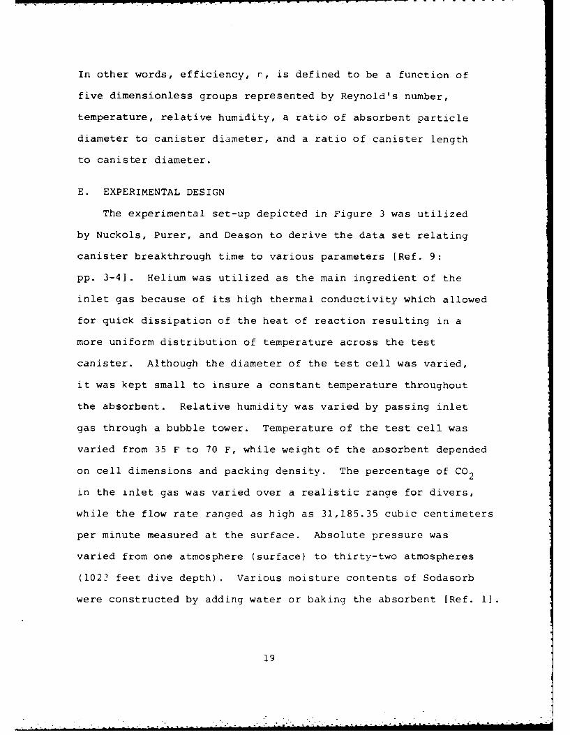
E. EXPERIMENTAL DESIGN

The experimental set-up depicted in Figure 3 was utilized

by Nuckols, Purer, and Deason to derive the data set relating

canister breakthrough time to various parameters [Ref. 9:

pp. 3-4]. Helium was utilized as the main ingredient of the

inlet gas because of its high thermal conductivity which allowed

for quick dissipation of the heat of reaction resulting in a

more uniform distribution of temperature across the test

canister. Although the diameter of the test cell was varied,

it was kept small to insure a constant temperature throughout

the absorbent. Relative humidity was varied by passing inlet

gas through a bubble tower. Temperature of the test cell was

varied from 35 F to 70 F, while weight of the aosorbent depended

on cell dimensions and packing density. The percentage of CO 2

in the inlet gas was varied over a realistic range for divers,

while the flow rate ranged as high as 31,185.35 cubic centimeters

per minute measured at the surface. Absolute pressure was

varied from one atmosphere (surface) to thirty-two atmospheres

(1023 feet dive depth). Various moisture contents of Sodasorb

were constructed by adding water or baking the absorbent [Ref. 11.

19

range of the dimensionless groups. Since the number of dimen-

sionless groups is less than the original number of variables,

considerable time and expense is saved during the process of

experimentation [Ref. 81.

Canister efficiency, n, was defined as a ratio of actual

breakthrough time, tBI to theoretical breakthrough time,

tTH: n = tB/tTH. Theoretical breakthrough time is computed

by dividing the absorption capacity of the chemical absorbent

by the rate of CO 2 delivered to the canister as follows:

A WtTH =QCCTH Q C C O 2

where:

A = mass of CO2 absorbed per mass of absorbent;

W = mass of absorbent;

Q = absolute volumetric flow rate;

C = CO 2 volume fraction in gas stream at depth;

DCO 2 density of CO 2 at depth for given temperature.

The dimensional analysis resulted in an expression for canister

efficiency, n, of:

= f(ReD,T,H,e/D,L/D)

where ReD is the Reynold's number and is defined as:

Re P Ve

D

18

TABLE 3

PARAMETERS OF CANISTER CO 2 ABSORPTION

Parameter Identification Dimensions

r-B Breakthrough time t

V Gas stream velocity L/t

T Gas temperature T

p Gas density m/L3

Gas viscosity m/Lt

C CO2 concentration L3/L3

H Gas stream water vapor L3 /L3

content

HA Absorbent water content L3 /L3

W Absorbent mass 0

e Particle size L

L Canister length L

D Canister diameter L

Dv Maas diffusivity L2/t

A Absorption capacity a/m

R Reaction rate a/t

Basic Units

t = Time 0 = Mass

L = Length T = Temperature

performed, the theory of which is described in Reference 8.

Dimensional analysis is useful when the variables involved in

a process are known, but the relationships among the variables

aie not known. If the variables can be reexpressed by only a

few dimensionless groups, then relationships between the groups

can be derived which are applicable to all cases within the

17

... . . .. , .. . ,. i . . ,., , .• ., -, ,. .. , .-. .-- : ..- ,-,,- ,. .:;,..:m , ;_ ..:,, m . . ._ i i . < ,.?

chemical absorbent. This radial movement of gas is a function

of the CO2 concentration, the mass diffusivity of CO2 the

distance from the centerline of the canister to the absorbent

surface expressed in terms of canister diameter and absorbent

particle size, and the turbulence in the gas stream as a

function of gas density and viscosity [Ref. 1].

As discussed earlier, water is necessary for the completion

of the absorption process and may be provided in the form of

water vapor in the exhaled gas of the diver or in the chemical

absorbent itself. Once the chemical absorption process has

been started, the reaction rate must be fast enough to keep up

with the rate at which CO 2 is arriving. The reaction rate of

the process is highly influenced by temperature [Ref. 1].

Table 3 lists the various parameters of interest, which,

although not all inclusive, were presented in Reference 1 as

having the most influence on canister duration. As the table

depicts, canister duration is then a function of fourteen

variables:

t = f(V,T,p,p,C,H,HA,W,e,L,D,A,D ,R)*B v

This functional relationship was simplified by observing

that the absorbent's reaction rate (R), capacity to absorb

CO2 (A), and moisture content (HA) were beyond the control of

the user, reducing the number of independent variables to eleven.

Next, a dimensional analysis of the resulting relationship was

16

S

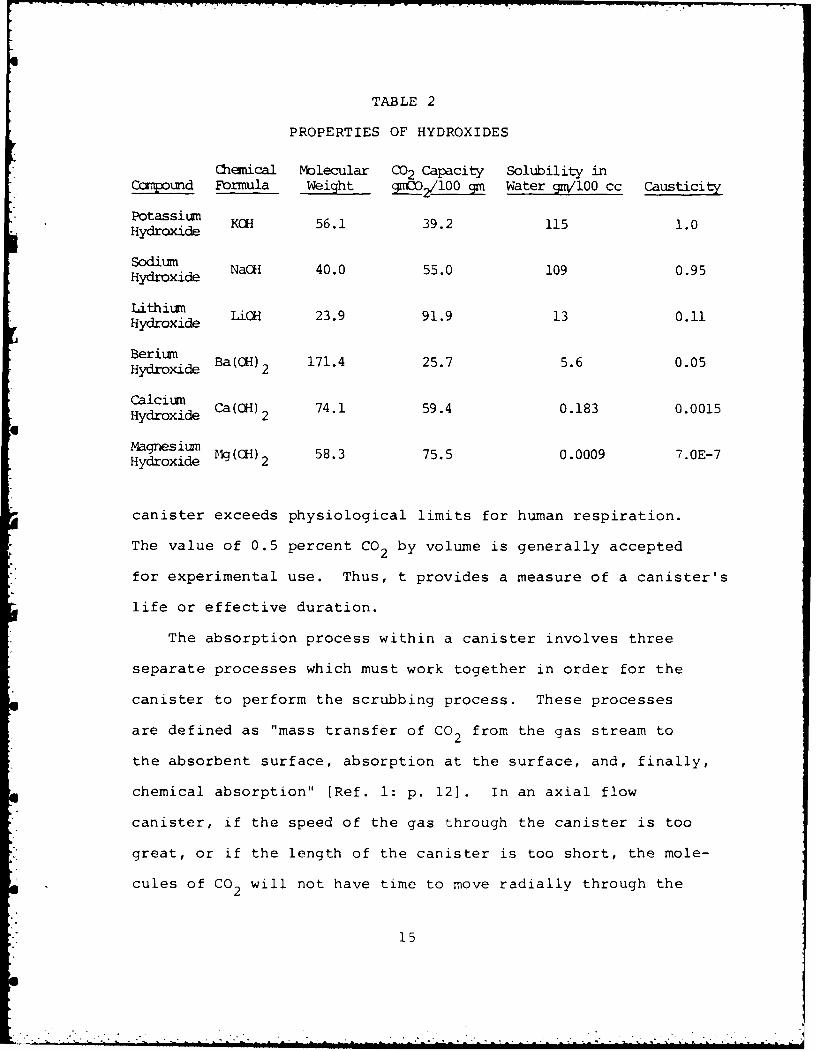
TABLE 2

PROPERTIES OF HYDROXIDES

Chemical Molecular C02 Capacity Solubility inCczmound Formula Weight g2/I00 m Water g/i00 cc Causticity

Potassixn1.Hoxide KCH 56.1 39.2 115 1.0Hydroxide

SodiumHydide NaCH 40.0 55.0 109 0.95Hydroxide

Lithitinhide LiOH 23.9 91.9 13 0.11Hydroxide

Beriumy Ba(OH)2 171.4 25.7 5.6 0.05

CalciumHydroxide Ca(OH) 2 74.1 59.4 0.183 0.0015

Magnesium mg (CH) 58.3 75.5 0.0009 7.OE-7Hydroxide 2

canister exceeds physiological limits for human respiration.

The value of 0.5 percent CO 2 by volume is generally accepted

for experimental use. Thus, t provides a measure of a canister's

life or effective duration.

The absorption process within a canister involves three

separate processes which must work together in order for the

canister to perform the scrubbing process. These processes

are defined as "mass transfer of CO 2 from the gas stream to

the absorbent surface, absorption at the surface, and, finally,

chemical absorption" [Ref. 1: p. 121. In an axial flow

canister, if the speed of the gas through the canister is too

great, or if the length of the canister is too short, the mole-

cules of CO2 will not have time to move radially through the

15

while excessive moisture will tend to flood the canister, block-

ing the critical contact between the CO2 laden gas and the

chemical absorbent particles and also, inhibit or slow down the

reaction. Nuckols, Purer, and Deason report that, "the moisture

content in the canister can change during its use due to an

imbalance in the water content of the incoming and outgoing

gas streams. Gas saturated with water normally would result

in an increase in moisture; however, if the heat of reaction

is not dissipated, high temperature areas will result in the

evaporation of water from certain sections of the canister thus

rendering such zones ineffective for carbon dioxide removal"

[Ref. 7: p. 59].

Although various hydroxides are available for use as chemi-

cal absorbents, the U.S. Navy has decided to use absorbents

based on calcium hydroxide. Table 2, comprised of data from

Reference 1, lists various hydroxides along with various

properties. It is of interest to note that while calcium

carbonate does not perform as well as lithium hydroxide, its

causticity relative to potassium hydroxide is lower.

D. PARAMETERS OF CANISTER CO 2 ABSORPTION

This section is a brief overview of the work of Nuckols,

Purer, and Deason [Ref. 1] in identifying the most important

or influential variables in the prediction of canister break-

through time, t. Canister breakthrough time is defined as the

time at which the CO 2 concentration in the gas exiting the

14

Sodasorb, a registered trademark name [Ref. 6]. It consists of

calcium hydroxide, 14 to 19 percent moisture by weight, less

than five percent sodium hydroxide, potassium hydroxide or

barium hydroxide, and ethyl violet as a sensitive acid/base

indicator. Ethyl violet is added to the composition to indi-

cate whether the absorbent chemical has been used or not. As

the CO2 is absorbed, the resulting pH change causes the granules

to turn from colorless to blue.

The actual process of CO2 removal by Sodasorb is a chemical

reaction. The CO2 forms carbonic acid which combines with

hydroxide to form sodium carbonate and water. Sodium carbonate

then reacts with lime to form calcium carbonate. The entire

process is characterized by the following equations [Ref. 7:

p. 58]:

CO + H 0 H CO2 2 +- 2 3

2H2CO 3 + 2NaOH + 2KOH Na2CO3 + 4H20 + K 2CO 3

2Ca(OH) 2 + Na 2CO 3 + K2CO 3 2CaCO 3 + 2NaOH + 2KOH

It is important to note that the chemical reactions will reach

their completion provided that the CO 2 laden gas remains inside

* the canister long enough and adequate mass exchange can be made

between the absorbent and the gas. Although water is a byproduct

of the above process, water is required to initiate the above

reactions. Insufficient moisture will then inhibit the process

13

6.00

4.00 Zone 1. No effectsZone II. Minor perceptive

3.00 changesZone II. Distracting discomfort

2.00 Zone IV. Dizziness, stupor,unconsciousness

.01.00Ao Partialo.9o-0 Pressure

<0atm, CO 20.60

0.40

, 0.30

~Tolerance zones fromr Figure I for 60-minute

0.10 1000 ppm e p s r0.08

0.06500 ppm

0.04

0.03 300 ppm

dll ~~~~ ~~0.02I10 20 30 40 60 80 100 200 300 400 600 800 1000 2000

Depth (ft)

Figure 2. CO Tolerance Zones

In closed-circuit dive systems, all exhaled gases can be

rebreathed by passing the exhaled gas through a canister con-

taining a chemical Co 2 absorber before the gas is inhaled.

Oxygen that is used in the process of metabolism is replaced

by oxygen from a bottle carried by the diver.

C. CHEMICAL PROCESS OF CO 2 ABSORPTION

The CO 2 absorbent used throughout the studies conducted

•at Naval Coastal Systems Center was High Performance (HP)

o- ' • 1

- 0.06- " [ - "" - '. "L '" ... .5 0 0 p p m " . . " " " "

ere the bar denote a sample average, the sum of squares due

co regression can be defined as

2SSR = (SYY - RSS) = (SXY) /SXX

In simple regression, the degrees of freedom (d.f.) associated

with SSR is one.

The coefficient of determination for multiple regression

is defined as F = SSR/SYY and represents a scale free one-

number summary of the strength of the relationship between the

X and Y of the data. It is easily interpreted as a percentage

of variability in the criterion that is explained by the model.

It also is the same as the square of the sample correlation

between X and Y. R2 has long been used to compare models of

the same data and its value in comparisons will be discussed

later.

Multiple regression implies that two or more predictor

variables are used to model the response variable. The basic

model is: Y = a + 3 1X1 + c2X2 + ... + 3 kXk + e where a and 2

are unknown parameters, e represents statistical error, Y is

the response variable and the X's are the independent variables.

The "real world" geometric interpretation of this model breaks

down as it is the equation of a K-dimensional hyperplane in

(K+l) dimensional space.

Analysis of variance (ANOVA) -rovides a method whereby

the fit of various models to the .ame set of data can be

26

compared. The F statistic is defined as F = MSR/RMS, where

MSR is the regression mean square obtained by dividing SSR

by d.f. and RMS is the residual mean square obtained by dividing

RSS by d.f. It compares the variation due to regression to

variation due to error. The F statistic is used to test the

hypothesis that all of the regression weights in the model are

equal to zero. If the calculated F value exceeds the tabled

value with the appropriate degrees of freedom, then one can

be at least 100(l-)% sure that at least one of the predictors

is significant [Ref. 12]. The significance level is represented

by cc.

22The coefficient of determination, R 2 , is now defined as

R2 = ((SYY-RSS)/SYY) = (SSR/SYY) and is the same as the square

of the multiple correlation coefficient between Y and the X's.

Most importantly, R is the square of the maximum correlation

between Y and any linear function of the X's, i.e., the pre-

dicted values of Y. Table 5 provides a summary of ANOVA for

multiple regression where K is the number of predictor variables

and N is the number of cases or trials.

TABLE 5

ANOVA FOR MULTIPLE REGRESSION

Source SS d.f. MS F

RegressSSR K MSR = SSR/k MSR/RMS(Xl,X 2 ... .Xk)

Residuals (error) RSS N-(K+l) RMS RSS/(N-K-l)

Total SST = SYY N-1

= RSS + SSR

270 .

Si- "e the calculation of R2 is dependent on the data set

from wnich the model was constructed, R2 associated with the

22

development sample will tend to be larger than R2 for the

population. This has led to the definition of adjusted R2,

2 2RA which is an attempt to correct R to more closely fit the

population. Adjusted R2 is defined as

RA R2 _ ((P(I-R 2 ))/(N-P-l)

where N is the number of cases and P is the number of predictor

variablis in the model [Ref. 13: p. 97].

Lane has defined the terms overfit and shrinkage to explain

the facts that R2 for the equation development sample will be

2 ,2larger than R or the population (overfit), while R developed

from using a model to predict over a new sample will be lower

than R2 for the equation development sample (shrinkage) [Ref.

14]. His study proposes three shrinkage estimation formulas

identified by their authors as fc'lows:

2 i 1 [2) ( - ) ( - -Wherry: RA 1 - (1-E 2

2 2Nicholson-Lord: RA =1 - (-R

Darlington: I- - (-R ) [(N-I) (N-P-l)]! I (N+!),'NIA

[(N-2)/(N-P-2)]

where N is the number of cases, P is the number of predictor

variables, R2 is the coefficient of determination for the

28

S oA -%A

2 rpeetR 2 ajse cequaticn development sample and represents R adjusted fcr

the population. The Wherry formula can be shown to be equiva-

lent to the formula proposed earlier in Reference 13 for adjusted

2R2 . The three formulas are, from top to bottcm, increasingly

conservative. The Wherry formula was developed to estimate

the value of R2 to be expected if weights from a given sample

were applied to a large number of samples from the same popula-

tion. Nicholscn and Lord noted that the Wherry formula actually

estimates R2 for the population; i.e., the result expected if

population weights were applied to the entire population rather

than the result of applying a sample equation to the population.

Both the Nicholson-Lord and Darlington equations are derived

from equations developed for residual mean square and estimate

R2 resulting from the application of a sample equation to the

population [Ref. 141.

In simple regression, a t-statistic can be computed as

t = 3/Syix, and is used to test the null hypothesis that 6,

2or the slpe, is equal to zero. It is observed that t F

when d.f. = 1. In multiple regression, the t-statistic is

used to test the null hypothesis that any one regression weight

or coefficient estimate is equal to zero. The t-statistic is

calculated by dividing the estimate of the coefficient by its

standard error. This statistic is then compared to the tabled

t value with d.f. equal to N-K-l.

In order to place any validity on the results obtained

from ANOVA techniques, various assumptions are made concerning

29

the data and distribution of the error term. These assumptions

are discussed informally by Amick and Walberg [Ref. 15] and

more formally by Weisberg [Ref. 11] and Younger [Ref. 12].

There are basically five of these assumptions which will be

presented next.

1. The model is correctly specified. Every variable (bothdependent and independent) is in its proper form.Linear regression requires that the relationship ofthe response variable to the set of predictor variablesbe linear. If the relationship is actually curvilinear,then transformations of the data must be used totransform a theoretically nonlinear model to linearform.

2. The data are representative of the range over whichpredictions are to be made.

3. Each observation or trial can be considered to beindependent of the others.

4. The errors in the model are assumed to be normallyand independently distributed with zero mean and commonvariance.

5. The distribution of the possible values of the responsevariable must be normal about the fitted line for allvalues of the predictor variables.

These assumptions, as they apply to the data set predicting

canister life, will be discussed later in this chapter. The

actual technique of checking for inadequacies of a model is

called case analysis and is discussed next.

B. CASE ANALYSIS

The analysis of the correctness and suitability of a model

is called case analysis. In order to understand the technique

and to place the author and reader on common ground, it is

necessary to define various terms used as well as notation.

30

I-

r n. - . - - l| n q _ _

Weisberg defines studentized residual, ri, as the residual

divided by an estimate of its standard deviation. The advan-

tage of studentized residuals (SRESID) over residuals is that

that standard deviation of the r. = 1, for all i. The studen-1

tized residual is also used in the calculation of a t-statistic

to be used in a test for outliers. The t-statistic is calcu-

lated by

t. r ((N-K-)/(N-K-r2)1 / 2

1 1 1

where N is the number of trials and K the number of predictor

variables in the model. If the calculated statistic exceeds

the table value of critical values for the outlier's test,

given significance level a with degrees of freedom N, then the

hypothesis that the case is not an outlier is rejected with

confidence 100(l-a)%. Table D of Reference 11 is a table of

critical values for the outlier's test [Ref. 11].

Outliers represent data points that lie beyond the fitted

e-quation and consequently will not be predicted with much

accuracy by the model. They are easily identified in case

analysis by their large residual or studentized residual and

can be confirmed by the outlier's test previously discussed.

outliers can be the result of randomness of the data, experi-

mental error, or they might represent new and unexplainable

information. They can not be routinely deleted from the

analysis, but must be examined for the source of their

aberration.

31

The studentized residuals defin above represent a scaling

of residuals, so that cases which are located far from the

centroid of the data space result in increased residuals, while

cases closer to the centroid result in decreased residuals.

Cook's distance is defined using studentized residuals and is

used as a measure of the influence a single point has on the

development of the model. The size or magnitude of Cook's dis-

tance will be determined by the magnitude of the studentized

residual and the distance of the point from the centroid of the

data space. A data point that exerts a large influence on a

model or fitted equation might have a small residual as it

essentially pulls the equation towards it, but can be identi-

fied by Cook's distance due to its position outside the centroid.

Highly influential cases should be examined in an attempt to

identify the source or cause of their uniqueness and, if deleted,

2will result in a lower value of R2 . However, more confidence

can be placed in the model in terms of its future application

[Ref. 111.

The single most important plot in case analysis is the

plot of residuals with the predicted values of the dependent

variable, Y. Weisberg recommends using studentized residuals

in the plot because each r. has zero mean and variance of 1 so

that 95% of the r. should fall within ±2 and 99% should be

contained within ±3 [Ref. 111. The plot should exhibit no

characteristic trends, i.e., should be a random scatter of

points about the axes. Such a plot would support the assumptions

of linearity of the model and common variance for the errors.

32

th

The standardized residual (ZRESID) for the i case is

defined by Norusis as the residual divided by the sample

standard deviation of the residuals [Ref. 13]. It is useful

in examining the assumption of normality of the errors of the

model. As with the studentized residuals, 95% should lie

between _2 and 99% between ±3. Additionally, a normal proba-

bility plot can be used as a check to see if the residuals

represent a homogeneous sample from a normal distribution. The

closer the plot resembles a straight line, the more certain

one is that the distribution of residuals is normal. If the

distribution is not normal, then a possible remedy is a

transformation of the dependent and/or response variable

[Ref. 11].

C. PROCEDURES FOR SUBMODEL SELECTION

Once the set of predictor variables has been defined and

appropriate transformations of the data have been made, the

next step is to select that combination of variables that pro-

vides the best model. The number of possible models to examine

is obviously based upon the number of predictor variables

available. If that number is large enough, a factor analysis

is appropriate to construct a smaller set of factors that are

combinations of the variables and essentially reduce the data

set to the relevant dimensions of that set.

With the computer it is possible to search through a large

number of variables to select subsets of those variables as

possible models. One method of subset selection is called

33

stepwise regression for which three algorithms exist; forward,

backward, and stepwise. The main advantages of these algorithms

are that they are fast and relatively easy to compute. They

do not provide a "best" model, but examine subsets following

a systematic technique. The three methods of stepwise regres-

sion are discussed by Weisberg [Ref. 11] and proceed as follows.

The forward selection algorithm first selects the indepen-

dent variable with the highest sample correlation with the

response variable. The next independent variable added is

chosen by the following three equivalent criteria: 1) among

the remaining variables, it has the highest correlation with

the dependent variable, adjusting for the independent variable

already chosen; 2) its addition will yield the largest increase

in R2 of the remaining variables; and 3) its t-statistic is

largest of the remaining variables. Forward selection can be

stopped by the following rules: 1) stop when a limit on the

number of independent variables is reached; 2) stop when the

significance level of the t-statistic for the remaining varia-

bles exceeds a pre-set value; 3) stop when the addition of

another variable would make the set of predictor variables

too collinear. Collinearity is considered by computing a

linear regression of the independent variable of interest with

the variables already in the model. R2 for this regression is

2computed and tolerance is defined as 1-R2 . If the tolerance

is less than some pre-set value, then the procedure stops.

The drawback to this method is that a variable selected early

34

in the model development may become non-significant and yet

remain in the final model.

The backward elimination algorithm starts with a model

constructed with all of the independent variables and then

removes the variables one at a time. The variable removed is

the one having the smallest t-statistic. Stopping rules are:

1) stop when the number of independent variables specified

are remaining or 2) stop if the significance level of the

remaining variables exceeds a pre-set value.

The stepwise procedure is actually a combination of the

forward and backward methods. It selects the first variable

as the one with the highest sample correlation. From then

on, it selects and ejects variables based on entry and removal

criteria set by the user and based on the significance level

of the t-statistic for the variable.

D. BUILDING THE MODEL

The New Rearession package of the SPSS (Statistical Package

for the Social Sciences) Batch System was used on the IBM 3033

to perform a regression analysis of the data in Appendix A.

The benefits provided by this package are: 1) a compute

statement that allows the computation of transformations of

the variables to provide a better fit, 2) the ability to use

the forward, backward, or stepwise algorithms for model

selection, 3) an extensive case analysis and graphis capability,

which enable a check of assumptions.

35

Examination of the correlation matrix of Table 6 reveals

that diameter, flow, and weight are all highly correlated.

The correlation between diameter and weight is expected because

as the diameter of the test cell is increased, the amount of

absorbent that the cell can hold, increases. The correlation

of flow rate to diameter and weight appears to be a result of

the experimental manipulation of flow to represent various rates

for different dive profiles. Flow rates were kept relatively

low due to the small size of the test canister.

TABLE 6

CORRELATION MATRIX

RH TEMP WT TIME LENTH

RH 1.000 -0.032 -0.293 0.127 -0.108TEMP -0.032 1.000 0.093 0.122 0.050WT -0.293 0.093 1.000 0.081 -0.045TIME 0.127 0.122 0.081 1.000 0.192LENTH -0.108 0.050 -0.045 0.192 1.000LIal, -0.322 0.113 0.974 0.062 -0.093CO 0.043 -0.025 -0.015 -0.218 -0.140FLSW -0.249 -. 091 0.854 -0.086 -0.063PRESS 0.127 0.157 -0.109 0.084 0.016HYDRA -0.041 -0.085 0.060 0.111 -0.007

DIAM CO 2 FLOW PRESS HYDRA

RH -0.322 0.043 -0.249 0.127 -0.041TEMP 0.113 -0.025 0.091 0.157 -0.085W 0.974 -0.015 0.854 -0.109 0.060TIME 0.062 -0.218 -0.086 0.084 0.111LENTH -0.093 -0.140 -0.063 0.016 -0.007DIAM 1.000 0.044 0.850 -0.133 0.071CO 2 0.044 1.000 -0.025 -0.406 0.023FLOW 0.850 -0.025 1.000 -0.102 0.041PRESS -0.133 -0.406 -0.102 1.000 0.1011YDRA 0.071 0.023 0.041 0.101 1.000

Making the assumption t : the nine independent variables

are the predictors most affecting the dependent variable, time,

36

a regression of time with these nine variables produced an equa-

tion of the form

Yn= 0 + i iXi

with R = 0.234. The independent variables selected were C02,

LENTH, RH, DIAM, FLOW, HYDRA, and TEMP. Table 7 lists the

ANOVA table and variable coefficients generated by the regres-

sion program. Examination of the histogram and normal proba-

bility plot of studentized residuals reveals departure from

normality. A histogram of residuals is provided in Figure 4.

TABLE 7

ANALYSIS OF VARIANCE TABLE

SOURCE SS DF MS FGRANO WEAN 25761545.093 1REGRESSION 8997912.646 7 1285416.092 16.090RESIDUAL 29478974.041 369 79888.819TOTAL 64238431.780 377 170393.718THE SIGNIFICANCE OF REGRESSION - 1 .0000(SIGNIFICANCE: AREA UNER CURVE FROM 0 TO COMPUTED F)R SQUARE - .234

COEFFICIENT B/SIGMA(B) CONFIDENCE INTERVALTERM B SIGMA(B) T LOWER LPPERBO -414.684 133.426 -3.108 -677.112 -152.25681 -67.361 12.927 -5.211 -92,787 -41.93682 57.751 13.465 4,289 31.267 84.234B3 1.516 .325 4.661 .877 2.15684 120.644 17.218 7.007 86.778 154.50985 -.055 .008 -6.571 -.072 -.03986 11.945 4.762 2.508 2.579 21.311B7 3.472 1.542 2.252 .439 6.504

THE THEORETICAL VALUE FOR T AT THE 0.05 LEVEL AND 369 DF - 1.967

TIME = f(CO 2,LENTH,RH,DIAM,FLOW,HYDRA,TEMP)

37

0

CL

E-nLi

00z

-400 0 400 800 1200

RESIDUALS

Figure 4. Histogram of Residuals

The plot of residuals versus predicted values in Figure 5,

reveals structure and suggests that a transformation of data

is required.

Examination of Figure 6 reveals that the distribution of

TIME is positively skewed and that the natural log transforma-

tion of time, LN TIME, more closely represents a normal

distribution. Conseqi:ently, the next step was to regress

LN TIME with all of the variables. This results in an equation

of the form:

38

0D o0

U1

Ddo

-40 4000

PRDCE TIM IN IN

Fiur 5. Plot of Reidal vs rdce

39.d*

: ~ ~ ~ ~~ - - - -am - - - -- ml . a ,,_ .,

or more appropriately

LN TIME = 0 + LN FLOW + LN WT + LN CO0 '2 1

+ LN PRESS + 5 LN RH + LN TEMP)

Setting 30 = ;n K, where K = exp(30 ) , the above equation can

be transformed to

P ' ' 4 V 5 6

TIME K(FLOW) (WT) (CO2 ) (PRESS) (RH) (TEMP)

which is a multiplicative model. The ANOVA table of Table 12

demonstrates that all coefficients remain significant at the

0.0001 level.

TABLE 12

ANALYSIS OF VARIANCE TABLE

ScA(PCE SS OF MS FCRAND LAN 4524.367 1REGPESSICN 319.147 6 53.191 366,335RESIDUAL 26.281 181 .145TOTAL 4869.794 188 25.903IWE SIGNIFICANCE OF REGRESSION - 1.0000(SIGNIFICAfACE: AREA UNDER CURVE FROM C TO COWUTED F)R SQUARE - .924

COEFFICIENT B/SIGMA(B) CONFIDENCE INTERVALTERM B SIGMA(9) T LOWER UPPER80 6.128 .713 8. 589 4.720 7.535B1 -1.551 .037 -41.886 -1.624 -1.478B2 1.623 .048 33.874 1.528 1.717B3 -1.609 .069 -23,160 -1.746 -1.472B4 -1.684 .084 -19.997 -1.850 -1.518B5 .060 .005 12.290 .050 .06996 1.234 .173 7.143 .893 1.575

THE THEORETICAL VALUE FOR T AT THE 0.05 LEVEL A) 181 OF - 1.974

LN TIME : f(LN FLOW,LN WT,LN CO 2 ,LN PRESS,LN RH,LN TEMP)

53

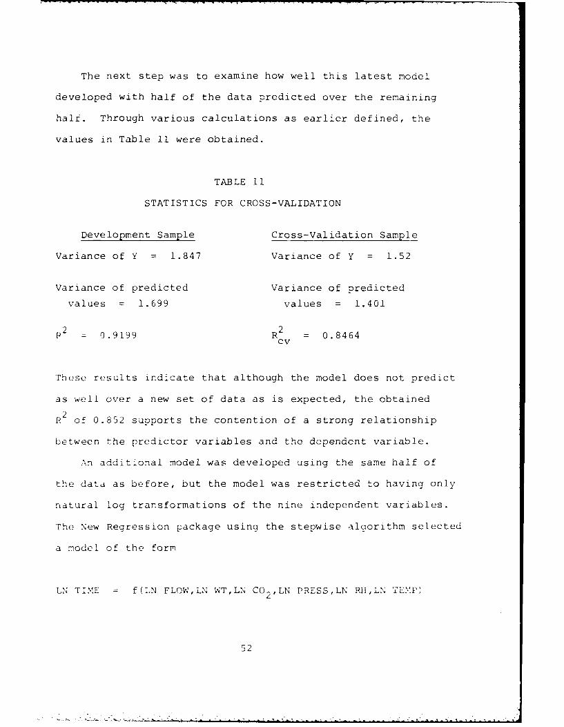
The next step was to examine how well this latest model

developed with half of the data predicted over the remaining

half. Through various calculations as earlier defined, the

values in Table 11 were obtained.

TABLE 11

STATISTICS FOR CROSS-VALIDATION

Development Sample Cross-Validation Sample

Variance of Y = 1.847 Variance of Y = 1.52

Variance of predicted Variance of predicted

values 1.699 values = 1.401

2 2P : 0.9199 R = 0.8464cv

These results indicate that although the model does not predict

as well over a new set of data as is expected, the obtained

R2 of 0.852 supports the contention of a strong relationship

between the predictor variables and the dependent variable.

An additional model was developed using the same half of

the data as before, but the model was restricted to having only

natural log transformations of the nine independent variables.

The New Regression package using the stepwise alorithm selected

a model of the form

LN TIME f(LN FLOW,LN WT,LN CO 2 ,LN PRESS,LN RH,LN 'iEMP)

52

C * • • 1t , • (

0 •*

0T • "

0 *,, *.. a CC • t 5* * * C

0 * .0• *1 S

C * , * •L en C * C

o •* *• *ee

* CC

NAUA LO T*M

Figue 13 Plt ofLN T ,I vs.Predcte

05

. . . . . .. - , -, .+ - - - , - - • . " - - - • : 2C-. d ra , m . -mC

Returning to the model developed during cross-validation,

the normal probability plot and residual plot of Figure 11

support the assumption of normality of errors. The plot of

residuals versus predicted values in Figure 12 shows little,

if any, structure.

0

C,

c/)00z

-1.0 -0.5 0 0.5 1.0RESIDUALS

Figure 11. Histogram of Residuals

The plot of actual values versus predicted in Figure 13 sup-

ports the assumption of common variance of the residuals.

Examination of the ZRESID or standardized residuals reveals

that 99% are within 3 and, therefore, support the contention

that residuals or errors are normally distributed.

50

I I I- -I - - -. .- - .- - r w. -.- . . . .

coefficient is small. The column labeled BETA, represents

the standardized regression coefficients derived by multiplying

the variable coefficient by a ratio of the standard deviation

of the independent variable to the standard deviation of the

dependent variable [Ref. 133. The actual coefficients do not

represent the importance of the variable in the regression

equation, since the independent variables are not expressed

in the same units. The BETA weights when standardized are

dimensionless, however, even then, they do not represent

importance since the predictors are intercorrelated.

TABLE 10

ANALYSIS OF VARIANCE TABLE

SOURCE SS DF MS FCRA MEAN 4524.367 1REGRESSION 317.780 6 52.963 346.731RESIDUAL 27.648 181 .153TOTAL 4869.794 188 25.903THE SIGNIFICANCE OF REGRESSION - 1.0000(SIGNIFICANCE: AREA UNDER CURVE FROM 0 TO COMPUTED F)R SOOARE - .920

COEFFICIENT B/SIGMA(B) CONFIDENCE INTERVALTERM a SIGMA(B) T LOER UPPER80 10.317 .259 39.870 9.806 10.8281 680 .030 -22.340 -.740 -.620

82 -1.538 .038 -40.552 -1.613 -1.46383 1.625 .049 33.064 1.528 1.72284 .058 .005 11,687 .048 .06885 -.276 .034 -8.053 -.344 -.20986 .022 .003 6.750 .016 .029

THE THEORETICAL VALUE FOR T AT THE 0.05 LEVEL AND 181 DF - 1.974

LN TIME = f(CO 2 ,LN FLOW,LN WT, LN RH,LN PRESS,TEMP)

49

model can be tested by comparing standard errors or by using

the standard errors to calculate R2 for the equation develop-

ment sample (R2) and R 2 , for the cross-validation sample (R 2S cv

The difference of R 2 R2 was defined earlier as shrinkage byS cv

Lane [Ref. 14].

Based on the above discussion, the data set was split in

half using a random number generator and a regression of LN TIME

with all variables plus natural log, second order, and inverse

terms examined. This resulted in an equation of the form

LN TIME = f(CO 2 1 LN FLOW, LN WT, LN RH, LN PRESS, TEMP) + constant

with R = 0.91996. This model can be represented as

LN TIME = + CO + 3 LNFLOW + '3 LNWT + 2 LN R0 1CO 2 ~234

+ 5LNPRESS + 3 TEMP

or

TTME = exp(U0 + 1CO2 + 2 LNFLOW + 23 LNWT + LNRH

+ LNPRESS + TEMP)

and is exponential in form. Table 10 lists the ANOVA table

and variable coefficients generated by the regression program.

It is observed from the table that all coefficients are signifi-

cant at the t 0.0001 level and the standard error of each

48

to 1.0, the better the fit. However, R 2 is the square of the

sample correlation coefficient, R, which measures the strength

of the relationship between the predictors and response. The

range of R is from minus 1.0 to plus 1.0 with values between

minus 1.0 and zero representing inverse relationships and values

between zero and plus 1.0, direct relationships. Younger

proposes the following scale to represent the strength of the

relationship indicated by R [Ref. 12].

-1.0 -.5 0 +.5 +1.0

perfect moder- moder- moder- noder- moder- moder- perfectately ate ately ately ate atelystrong weak weak strong

inverse direct

For example, from the graph, an R 2 of 0.5625 would translate

to an R of 0.75 indicating a moderately strong relationship.

2The second question concerns the data dependency of R

Adjusted R2 can be calculated as previously discussed to

predict a value of R 2 for the population or the model can be

tested by examining how well it predicts with a new set of

data. Since a regression model is developed to fit a data set

as closely as possible, testing how well a model predicts over

this same data set is almost certain to overestimate performance

[Ref. 171. This idea has led to the notion of simple cross-

validation, where a data set can be split in half and the model

then developed over one half and tested on the other half. The

47

. -. -. . . - .' . ." ' - .. .. .

0 * 0

2 44

. t o e

Usn the stpws prcdrso e* Rgesoi a

only th e po v tt ar sc ad *

hihl corltd Tw quston rean however and t vae

deedn vaiale "and 2) ho"elwl odlpeitwt

2 2

deiito of R Bae on it deiiin th lsrR i

4 6 6

NATURAL OG T .*Fiur 0. Plo ofReiuasvs Peice

Usin th stpwsepocdue ofNwRgesoiSa

been pssibleto adjst thevalue of toeac n sgii

cacelee fo h t ~ tet so that there *lin moe ncue

onytos prdco vaibe*htaesinfcn n*o

highly crrelated Tw usin ean hwvr n hy e

i)hwl g*de 2 ne to bebfr* oelrpeet

44

- -; : , -,,,,,.-,.,,,.. . .,a .,.- - & -,, ,---"" %," 'a, - = m,' " " ' '- " " " - ; " "w " -" " -"4

00 C

z

-1.5 -1.0 -0.5 0 0.5 1.0

RESIDUALS

Figure 9. Histogram of Residuals

The residual plot (Figure 10) shows little structure, suggest-

ing the current model is adequate. The model is exponential

and can be expressed as

N

Y = exp(3 0 + 1 KiXi)

The set of predictor variables chosen in this final model were

selected from a set composed of the original nine independent

variables, plus square terms, cross terms, and both inverse

and natural log transformations of the independent variables.

45

,.. ; ".ii.- .',-ii-- Z. . .'ill-.-,,..i................................................................,.......-..'..,..'

with R= 0.880. Table 9 lists the ANOVA table and variable

coefficients.

TABLE 9

ANALYSIS OF VARIANCE TABLE

SOURCE SS OF MS FGRAND kEAN 8928.089 1REGRESSION 554.854 6 92.476 451.708RESIDUAL 75.748 370 .205TOTAL 9558.691 377 25.355THE SIGNIFICANCE OF REGRESSION - 1.0000(SIGNIFICANCE: AREA UNDER CURVE FROM 0 TO COMPUTED F)R SOUARE - .880

COEFFICIENI B/SIGiM(B) CONFIDENCE INTERVALTERM B SIGMA(B) T LOWER LPPERBO 10 155 1.65E-01 61.371 9.830 10.481B1 -1.540 3.13E-02 -49.225 -1.602 -1.478B2 1.583 3.77E-02 42.043 1.509 1.65883 -. 123 4.65E-03 -26.516 -. 132 -. 11484 .007 5.34E-04 12.616 .006 .008B5 .000 2.26E-05 7.117 .000 .000B6 -.016 3.36E-03 -4.627 -.022 -.009

THE THEORETICAL VALUE FOR T AT THE 0.05 LEVEL AM 370 DF - 1.967

2 2LN TIME = f(LN FLOW,LN WT,(CO 2) ,RH,TEMP ,PRESS)

All variables are significant at the 0.001 level as is the

developed equation. By calculating the t-statistic for an

outliers test as defined earlier it is observed that for case

126 with the largest studentized residual of 3.062, the t-

statistic is 2.9924. From the table of critical values for

the outliers test, t = 3.87 for a = 0.05 and d.f. of 369. This

implies that it is not 95% certain that case 126 is an outlier

and, therefore, no cases will be deleted. Examination of the

histogram of Figure 9 supports the assumption of normality.

44

-.. .* I." ... . ,- • - - " - - -, . .i.--..-., ,,- m ,, m l li 'lnl . ,I a d d

The current model is then an exponential model of the form

nY = exp( 0 + X .)

and the relationship between TIME and the predictor variables

is curvilinear. The equation is inherently linear as it is

possible to use the naturla log transformation to yield a

linear form

nZn Y = 20 + [ 3i9ii0

Examination of the case statistics reveals that case number 292

has a large value of Cook's distance of 0.2355 with the next

largest value equal to 0.04295. Since its studentized residual

is only moderately large, its influence is most likely large

and it is deleted for the purposes of further analysis. Case

292 is the case with the highest recorded flow rate and might

possibly represent failure of the model to predict over high

rates of flow.

Next, a regression of the natural log of time with all of

the predictor variables, plus second order terms and natural

log terms was run. In order to enable the calculation of a

natural log of RH, which at times is equal to zero, 0.0001

was added to all values of RH. Using the stepwise algorithm,

the regression yielded an equation of the form

2 2LN TIME f(LN FLOW,LN WT,(CO 2) RH,TEMP PRESS) + constant

43=6R PES)+cntn

0L

0n

0

0

0

0-2 0 20 RESIDUALS

Figure 7. Histogram of Residuals

<*

CN * %

NAUA LOG

Figue 8.Plo of esiualsvs.Predcte

:4

n= 0 + 3iXii=l '

where the variables selected are HYDRA, LENTH, WT, C02 , RH,

and FLOW. R2 has reduced to 0.218 as depicted in Table 8

which is the ANOVA table with variable coefficients. Both the

histogram of Figure 7 and the normal probability plot have

improved to support the assumption of normality of the errors

and most of the structure of the residuals has disappeared

(Figure 8).

TABLE 8

ANALYSIS OF VARIANCE TABLE

SOURCE SS DF us FGRAND MEAN 8928.089 1REGRESSION 137.544 6 22.924 17.203RESIDUAL 493.058 370 1.333TOTAL 9558.691 377 25.355IHE SIGNIFICANCE OF REGRESSION - 1.0000(SIGNIFICANCE: AREA UNDER CURVE FROM 0 TO COMPUTED F)R SCUARE - .218

COEFFICIENT B/SIGMA(B) CONFIDENCE INTERVALTERM 8 SIGUA(B) T LOWER UPPER80 3.613 3.29E-01 10.985 2.966 4.26081 .068 1.93E-02 3.528 .030 10682 .161 5.47E-02 2.943 .053 .268B3 .012 1.82E-03 6.704 .009 .01684 -.286 5.24E-02 -5.463 -.389 -.18385 .004 1.31E-03 2.836 .001 .00686 .000 3.46E-05 -6.034 .000 .000

THE THEORETICAL VALUE FOR T AT THE 0.05 LEVEL AN[) 370 DF - 1.967

LN TIME = f(HYDRA,LENTH,WT,CO2,RH,FLOW)

41

Y')

0

4

4

CL4P0

400

A standard error comparison shows that this multiplicative

model has standard error of 0.38105 versus 0.39085 for the

2exponential model. R 0.924 and the residual plot of Figure

14 is approximately normal, while the plot of residuals versus

predicted values is without structure, Figure 15.

0

0

zU--7_

-1.0 -0.5 0 0.5 1.0

RESIDUALS

* Figure 14. Histogram of Residuals

As with the exponential model, the plot of predicted values

* versus actual values generally supports the contention of

con-non variance of the errors, Figure 16.

A final approach to mrnlelling was made in an attempt to

-rovide the capability to make predictions beyond the range

54

019I

9I

o • • e * , **

T •9

,999 * I * 12 4 9*

NATRA LO9TM

FJ~gre ]5, Pot o 9Resdua9 9s Pe~ce

*%

9 9 9 , * ,* q9 9 $ 9 9

99 99•99 99 * •9 9•

* * :*99 *

"

,. A ".99.9.90. • •

o99

I 9 , I2 4 6NATURAL LOG TIME

Figcure 15. Plot of Res2Idual vs. Predcted

a9

:9!

of the current variables by using ansformations of the pre-

dictor variables to redefine the data space. The result of

the dimensional analysis discussed earlier was to identify

efficiency as a function of five dimensionless groups. This

expression can be rewritten to demonstrate that efficiency is

a function of eight variables: n = f(p,V,e, ,T,H,L,D). As

defined earlier, the theoretical breakthrough time, tTH , of

a canister can be calculated by knowing the weight of absorbent,

the flow rate, CO 2 concentration, and density of CO 2. Now,

7anister efficiency is defined as n = tB/tTH and can be calcu-

lated for each trial or case in the data matrix.

This approach is to build a model from half of the original

data set to predict efficiency, yielding tB from the product

of n and tTH. From the data set, it is possible to express

efficiency as a function of nine predictor variables:

n = f(RH,TEMP,WT,LENTH,DIAM,CO 2 ,FLOW,PRESS,HYDRA). Since

efficiency is not affected by weight of the absorbent, WT

may be removed from consideration. Of the remaining variables,

only FLOW, LENTH, and DIAM are restrictive in the sense that

they limit application of any model to small test size canisters.

However, by reexpressing LENTH and DIAM as a ratio and replacing

FLOW with mean linear gas velocity defined as V = FLOW/Acs,

where A is cross-sectional area of the canister, the predictorcs

set ranges over the full extent of practical applications.

Efficiency can now be expressed as a function of seven variables

as, f(RH,TEMP,L/D,CO2 ,V,PRESS,HYDRA). Examination of the

F 56

65

correlation matrix of Table 13 reveals that several variables

are negatively correlated, yet none are very highly correlated

with each other.

TABLE 13

CORRELATION MATRIX

RH TEMP LOD CO 2

RH 1.000 -0.091 -0.061 0.087TEMP -0.091 1.000 0.035 -0.032LOD -0.061 0.035 1.000 -0.162CO2 0.087 -0.032 -0.162 1.000VBAR 0.018 0.118 0.030 -0.113PRESS 0.217 0.144 0.030 -0.417HYDRA -0.038 -0.071 -0.012 0.021EFF 0.440 0.191 0.100 -0.275

VBAR PRESS HYDRA EFF

RH 0.018 0.217 -0.038 0.440TEMP 0.118 0.144 -0.071 0.191LOD 0.030 0.030 -0.012 0.100CO 2 -0.113 -0.417 0.021 -0.275VBAR 1.000 -0.024 -0.143 -0.362PRESS -0.024 1.000 0.097 0.183HYDRA -0.143 0.097 1.000 0.005EFF -0.362 0.183 0.005 1.000

After calculating efficiency as tB/tTH, it was discovered

that in 17 of the 188 cases, efficiency was greater than one.

These values were all changed to one as an efficiency greater

than one has no meaning and in this situation is most likely

the result of error in measurement. A regression analysis

was run with efficiency as the dependent variable and resulted

in an equation of the form

5Y + X.

i=l57I

where the predictor variables are, in order, RH, V, C0 2, TEMP,

and PRESS. The variable coefficients are 0.00346, -0.64302,

-0.11180, 0.00983, -0.00740 with a constant term of -0.10873.

2R = 0.569 and all variables are significant at the = 0.01

level. Both L/D and HYDRA were not selected as they were not

significant at the 0.01 level. The residual plot of Figure 17

shows some structure suggesting that a transformation of data

might provide a better fit.

Fiur 17. Plo of Reiul"s rdce

LJpa-r fro nomliy Fiur 19 is a lt ofefcec

n58

0 -

, * *p

I * 1t-0.40 0. 0.8

Fiur)1. *o of Reiul vs. *dce

The ogrm o reiduas i Fiure18 idictesa sighr" *

Dp ar rmnraiy Fgr 19) isa0*tofefcec

0 * * **8

• ." , 'w . " ",, "m. ,In l - -- i 1 m I" m * * " * i "'o""Ou - " . .

0

C,

oi L LAL L I0z

InI

-0.4 -0.2 0 0.2 0.4 0.6RESIDUALS

Figure 18. Histogram of Residuals

0000 0 *

00. 0, 0. ,.0

Fir 19 Plo of Efiiec vs. Pre0cte

%. *059

0*00 * • Q *

UJ 00 • I

1*0 I I I J I

0? 0.4 0.6 0.8 1.0

EFFICIENCY

Figure 19. Plot of Efficiency vs. Predicted

59

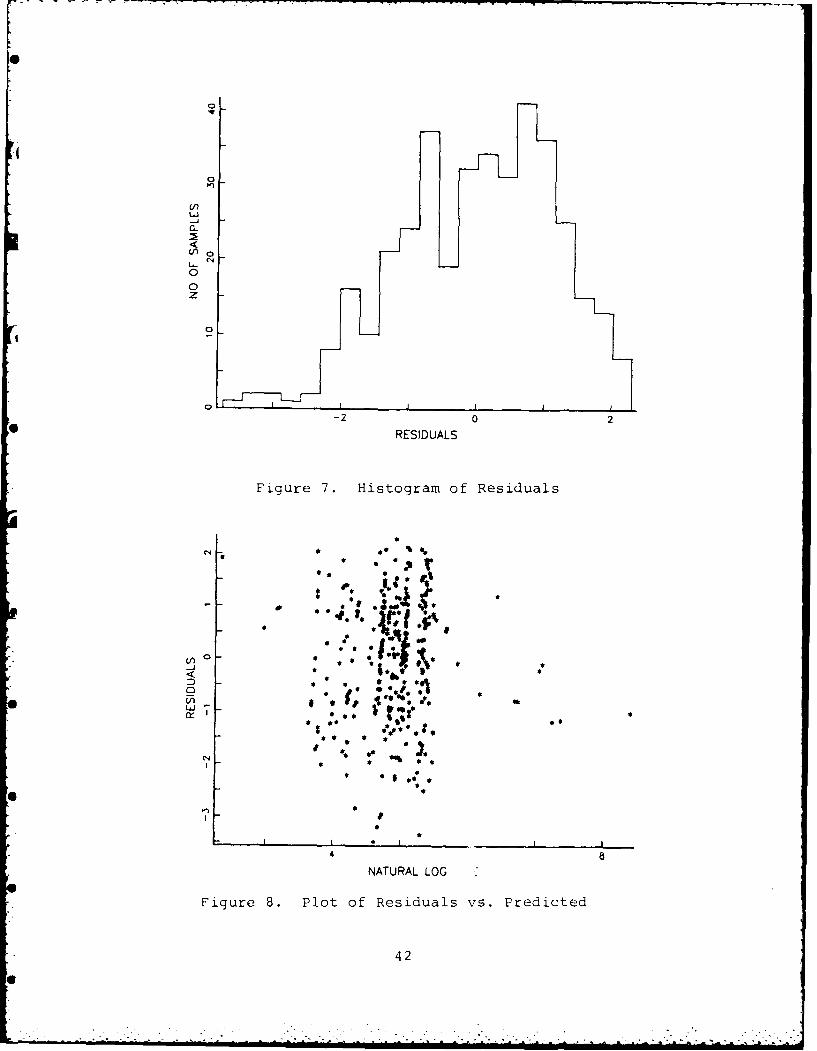
versus predicted efficiency and depicts the variability of

predictions over the range of the dependent variable.

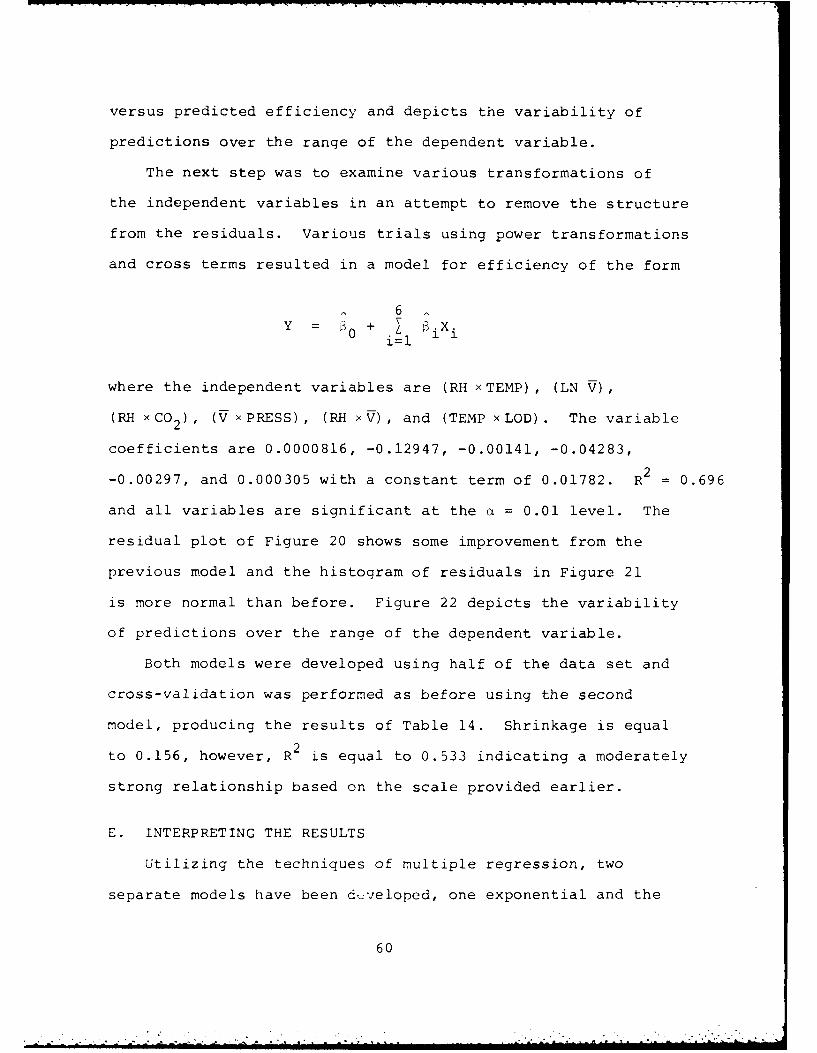
The next step was to examine various transformations of

the independent variables in an attempt to remove the structure

from the residuals. Various trials using power transformations

and cross terms resulted in a model for efficiency of the form

^ 6Y = + .X.

i= 1

where the independent variables are (RH xTEMP), (LN V)

(RH xCO2 ) , (V xPRESS) , (RH xV) , and (TEMP xLOD) The variable

coefficients are 0.0000816, -0.12947, -0.00141, -0.04283,

2-0.00297, and 0.000305 with a constant term of 0.01782. R = 0.696

and all variables are significant at the a = 0.01 level. The

residual plot of Figure 20 shows some improvement from the

previous model and the histogram of residuals in Figure 21

is more normal than before. Figure 22 depicts the variability

of predictions over the range of the dependent variable.

Both models were developed using half of the data set and

cross-validation was performed as before using the second

model, producing the results of Table 14. Shrinkage is equal

to 0.156, however, R 2 is equal to 0.533 indicating a moderately

strong relationship based on the scale provided earlier.

E. INTERPRETING THE RESULTS

Utilizing the techniques of multiple regression, two

separate models have been d,veloped, one exponential and the

60

0

0 0 0. 0. 0.8

W , * **, * ,

, S * * *

* * I S I I * S

4

0 0.2 0. 0.6 0.

0

0S

l.

-0.4 -0 2 0 0-2 0.4

RESIDUALS

Figure 21. Histogram Of Residuals

61

• '' ' "' - . " "--' ' -- - " i & " * " . ."' - . .S; ' : -- '

Z %

0 * *

LJS

* * * * *

0. 0. . . .

* - *

DvlpetSaml cross-Vldto Saml

00 * 'I *

v r i o Y. =. 0 6 V.07

0ariancef iredicte 22. t p Eredicted

values = 0.05989 values = 0.04376

R 2 =0.689 R 2 =0.533cv

62

" ,,,,-, 4 k w,,m ,I,,, I,,l, " " ".... . . ..~' . * • . * , . . . . .

other multiplicative, to predict the canister life, tB , of

an axial flow canister containing High Performance Sodasorb.

Both models have selected the same set of independent or

predictor variables to estimate tB' The variables chosen are

percent relative humidity of the gas stream (RH), temperature

in degrees Fahrenheit of the inlet gas (TEMP), weight in grams

of the chemical absorbent (WT), percent by volume, surface

level equivalent, of CO 2 in the inlet gas (CO2) , absolute rate

of flow of the inlet gas in cubic centimeters per minute (FLOW),

and absolute pressure of the environment expressed in atmos-

pheres absolute (PRESS). The variables not included are

canister length in inches (LENTH), canister diameter in centi-

meters (DIAM), and moisture level of the chemical absorbent

(HYRDA). Earlier examination of the correlation matrix revealed

that both length and diameter are highly correlated with both

weight and flow. Chemical hydration level is usually fixed by

the manufacturer and the results of this analysis indicate it

has small significance in predicting tB*

Both models have satisfied the assumptions inherent in

regression analysis as demonstrated by the case analysis.

All coefficients are highly significant and approximately

92% of the variability of the data is explained with each

model. However, the worth or value of these models lies in

their ability to predict canister life, tB*

As stated earlier, regression analysis provides a basis

for making predictions within the ranaes of the values of the

63

independent or predictor variables. This restricts the use

of the models to the ranges provided earlier in Table 4.

If a canister of known dimensions is filled with HP Sodasorb

and subjected to a gas stream flow rate with known CO 2 concen-

tration and relative humidity at a particular depth and tempera-

ture, then the life of that canister can be predicted.

Predictions made outside the range of the data are suspect

and not reliable. This is demonstrated by the following example

calculations. The MK-12 surface surorted dive system utilizes

a canister 14.75 inches in length with a 6 inch inside diameter.

For a dive depth of 390 feet (12.82 ATA), a flow rate of 6.0

absolute cuvic feet per minute (acfm) is required of which 0.6

is utilized by the diver leaving 5.4 acfm to enter the canister.

A CO 2 level of 0.58% at the surface or 0.04524% at depth is

assumed to enter the canister. The weight of absorbent inthe

canister is 12 lbs. or 5448 grams, while the temperature is

600 F and the relative humidity is assumed to be 100%. Using

the exponential model, tB is predicted as 891 minutes or 14.85

hours. Theoretical canister breakthrough is calculated to be

1355 minutes or 22.6 hours. In actual practice, the MK-12

dive system has been utilized to slightly more than 10 hours

as reported in Reference 1.

Since the models generated are restricted in use to the

ranae of the values of the independent variables provided in

the data set, this limits their application to small test size

canisters that are too small for diving applications. In order

64

to successfully apply this analytical approach, additional

tests would have to be made with larger canisters, allowing

for greater absorbent weights and higher gas stream flow

rates.

The final approach of modelling efficiency as a function

of the data resulted in two models with R2 values of 0.569

and 0.696 respectively. Most importantly, this approach allows

tB to be calculated from the product of n and tTH over a much

larger data space than before. Sample calculations were per-

formed for the MK-12 dive profile as previously discussed for

both models. The variable values were as follows: RH = 100,

V = 0.46, CO 2 = 0.04524, TEMP = 60, PRESS = 12.82, L/D = 0.9678.

The first model predicted an efficiency of 0.431 yielding a

canister breakthrouah time of 584 minutes or 9.7 hours. The

second model predicted an efficiency of 0.230 yielding a

canister breakthrough time of 311.7 minutes or 5.2 hours.

Recall that canister breakthrough of approximately 10 hours

has been observed in actual practice for this MK-12 dive

profile. The ranges of the variables used in the model develop-

ment are listed below, defining the space over which application

of these models is restricted.

MEAN VAR MIN MAX

RHI 61.7 2215 0 100

V 0.2067 0.0446 0.0219 1.465

CO 2 1.1445 1.3295 0 .031 4.35

Tk.*P 66.9947 84.6363 35 80

PRESS 4.1277 48.5291 1 32

P 2.6606 2.9050 0.2514 16.36

65

III. CONCLUSIONS

The CO 2 absorption process in a canister is a chemical

process requiring both water and heat in order to perform.

Water is provided in the chemical absorbent and in the moisture

of the gas stream. The process is highly influenced by the

rate of flow through the canister, the concentration of CO 2

in the inlet gas, the moisture content of the inlet gas, the

operating temperature and, to some extent, the operating

pressure. The effect of pressure is to change the density

and viscosity of the inlet gas and more importantly to affect

the actual water content of the gas stream [Ref. 1].

The models generated to predict canister breakthrough time

appear to meet the assumptions inherent to multiple regression

analysis and explain approximately 92% of the variability of

the data. Their application is limited however to axial flow

canisters with steady flow and, most importantly, to small

canister dimensions. In order to utilize this approach of

modelling canister breakthrough as a function of the available

data and be able to apply the model to a wide range of canister

sizes, more experimentation would be required.

Utilizing the definition of theoretical canister life and

canister efficiency provided in Reference 1, canister efficiency

das calculated for each of the 188 trials representing half

Df the data. Canister efficiency was then modelled as a

66

function of the eight independent variables. By reexpressing

gas volumetric flow as gas mean velocity and reexpressing length

and diameter as a ratio, the ranges of the independent varia-

bles in the development sample include parameter values for

most dive profiles. The models for efficiency in Chapter II

explain approximately 60% and 70% of the variability of the

data, respectively. Simple cross-validation has shown that the

models, while showing the expected shrinkage do exhibit good

stability across different data sets.

These models should serve as an aid to the design process

outlined in NCSC TECHMAN 4110. As models, they represent an

attempt to quantify the relationship of canister performance

with variuous environmental and geometric parameters.

67

.. . .= . .. . I -. - - - 8 .. . . .. . .. .. . .. . •

0

APPENDIX A

iDATA

1-- 4 44- "44 41 4 -r 44-44 4..-.44-4 .. 4-4 -4.4 -4 .-4..4e~ * g...... 0 00 *00 00 0*0 0 0S g0... 60 0 Ce e * g.

-4-4 4.4-- 444-4 4

itlci 0 -i a m -L~n-(7 G OCDON4 lor'.A 0L-.i~nunLA)OC'JNa~tor--4Nq 0 *0000 000a00 00*00 O

LL rr. 0NrvOO' 0-04 C%, 1 00 ON 0 q~- j % 0 v .rcG

JX 0 mzm000mm -m o wmw 000.4MM OO-4rOA~fOMMaO'r-mmo mmm lmmoa

m aX o c CD o cDC o a o Co CD oo o o o o ~ Co c CO (3 Co00 3 CIO 00 Co 00 co 00C 00 C0 CO 0 00 00 Co Co Co 00 G o co co 0Co0

t ttn4 loi r UW'J.O

ZLnr~v1,7 anAnm40-vu-4. tOOLuO touLin--Ln.O4o-toAOrLALn hntLnf.

rf-4)'o \ or- ojecpcoq coo ooor-.CooONNo~nj .o -4 ONO 40-~o 0

SLA .-4-4 (~%J-4 rn -404 ~ .4N NN ... LA...4 r'.J-4N

0 00 00 0O0 LACNLn )II n A U LAU\LA00C000 )0 0 oC0 CO0 000 00 00 00

68

e. .s 0 *eeO4 60006664 see .... so.- 4eo e o 0 .06

0 coot 00000I0a, t00n0LIN000000000000 00000000o-,

00O~N0004'000o00OoAn

~~~- m mcf-Nf

c7%~U c-I -4 N-4 4- o'f%~. %0%oaa- %O%U NC'J(\JNCNI r. -44 .- 4r-r

M 00o0O0m0oOw0000000OcOac0OOO0~~nO0OCOC0CC00OO OO AWCOC00

0000000000Zonr-000000000000000000000Oo oc,00000000000000-t t-q~

OQ~~~OQ~~C~~N N NN N0 0O 0N' ' Q' O N

000~a m n-0 00

-4 4-44,44--

~6

r

00000(. r-4 00 t00 0 t0O00000 0 0 o s0r0 (7O00 (%o0 000 o00

w.ocowao3 zwm0 6 oao6 w00 c ma a 0 0 6 00:) *00 0 00 OW0W00 0 00 00 300 0.0..w000CCCoWCwW

N -4c~i*r 0tr(J (4 N %C,4JCjC\Ci 0%JNC4 NC4 NNN N N %C\ NN C4NM\N NrMCj

V\4 fn 0 -- C400%4 Ln C.J.-4 '- .4 -4 .N- N.N,0o -4w(4.n-4L ,r'JN-4 144 4

n*J f ' (3oo (ou\0 0o((L00ADo0000~n ooo00o4. noo00o 0

0000666 0000=000006006000000600000 00000660000000

0 0 0 0 0 0 *0 0~ N O 00900000

m0m000 t6t0 mMt00m000t60T 46000t00t0t. 66 r60006 t606t6t60060666r0t004 -

mNN mJN% Nm N low N N NNcJNN N NNeJc~c'NNN'

00-ALO0 %O O ONnr cgU~O O O~-.O OJ

07

00 0000000r-0000 0000 000u00000 0000lu)00000000000% 00000 U1% 000lLlU~(T

ege ee 00 000e eeg eg0e ege ego..... eooca e..g0ee0e ge~DDCM 0 00COO O~DDOVQO OO DO O OD

0%0 % %0 % J % %0 t %0 % %0 0 %0 U %0%9 3 a O0 0 %G 0 %a'0 % J % 4 %(7 %a U %V%0 .

(14 In NM O 4%n 0)N N~ NN O-(nr-4000 -4..OO'-t 4( -4 N 4r

~., ~N NNNNN NNN N -4 -4- 4O

Ln~c Lno rr-lrr rr0CCP p P lNlrr---r -r -r - -- P -- l

~~~coc71

g00 90 eg 0 Og~ e 0e0 0 090a Ogge 069 0 00 S O~~ Co ag e e

..4(n Ln(Wn.-4CS..4 *N4 Nt .4 -4,tMN IVNN0J-4NN Nao.O

,00Q m000,,,,0000 u'' '0' 1 LA00L A LAn(mn jn qnn~c (mL

O4-4n4(-tO--L.n'.OO.'or- m StOOOO-4qC-44T n NNNNN 4NNtNNtN4N4e. 0NNN4WM

-4 4 -U 4 4 44-4 4 - 44 r-4 e4 N-4- - O -444 -- 4 44, N4

-4-4 4-472

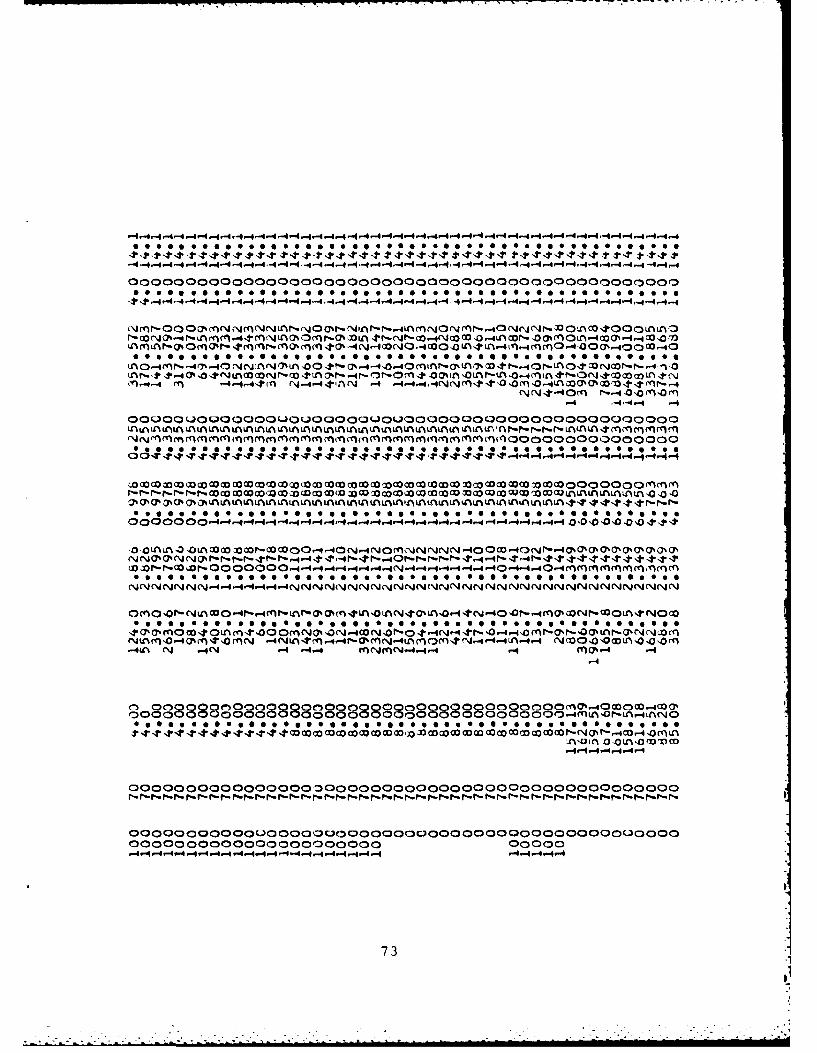
-. -W 444r4

~44- '4- ~-4.044 4-'- no - - 44-4,4.444.44~-- 4 414-4 -4-4f- I'4- I;4~ .- 4'-4-4 44

.0Jr-00L , n ~ ~ mOr~ N(o - o o () \ 0 N r' N 0 -4 N NN 04tfl- C-.O 40CJr - 0% O'cO '00 3%0%0%0%G

0 0 - 4-4 r4 . 4 4 4 -.- , N-AN- -4 -4r 40 40

-4A 4 4N-4 -44 NM-44 (o .4. -4 -

000~0004J0U0000 oooooo a000000000000000000000F~

N m (~~fl(''U I 0 -JO ) 00000M M000 0

See ge e eg e egg- geese.... rr-r - -P-P r - -P-P . g e Ie-- eges 5-P -r . 05* e.gg - -

Ooo

r-r.oo ~:0a~~zjg ~ ~ v i o73

4- 0 0 44 44,4 414114 4 -410-%I440. 4-4v

40-

mm ro-4- o o Qo Lnnnti~nLt~~ nnt~ nn~~vL ~nnn-r- r. r-r-

10.~4 Qr't-rrrt- t-r-t--

OO.,-~-~t -%N 0 OO00%(Jn-Or4CG 7% 00% 0000 000 -0000000000000N M

eggt megegeggen~ egego~ egg. oo Qwgeg owggggg g g.g g

74-

1- 000 -4106D0G0561 0064060606m004 *66*00M0@0M 60600006

~4N N N N N N- N N N

000000000000000000NO O4, ()-4 -00000% N'0 () o00r000 t0000000%,

M 00 o00oc 3 a o c 0 ~0O 0 00 0O 00O0 0 00O 0 0 000OOD00 o000o o a00OL

0 00 00 0 0 0* 00 00 0 * 0 ' 0 e 0 U'0'

0000000000000000000000000000000000000000000

0e * e e g0 0 00 0 00 0 9 0 0 0 0 0 0* ag05 sea gees 00

N N~ 0 N N~~ 4N-4 rn4.NcrcD'Inq~~~~~ ~ ~ ~ .-. 4 444 14 1 4N-O

0 *g 60 6 0 00 0 0 00 g0g ge 0 6*se eg0 66 00 0 66

75

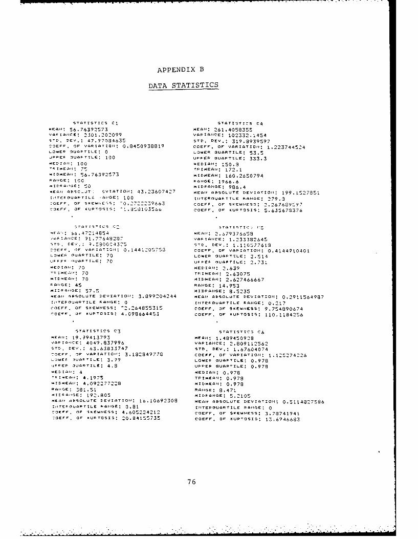
APPENDIX B

DATA STATISTICS

STATISTICS Cl STATISTICS C4

WEAN: 56.76392573 mEl: 261.4058355

V A ",.CE : 2301.202099 VARIANCE: 102332.1454ST.. DEV.: 47.97084635 STO. DEV.: 319.8939597COEFF. OF VARIATIOI: 0.8450938819 COEFFR OF VARIATION: 1.223744524LOWER 3UARTILE: 0 LOWER QUARTILE: 53.5UPPER QUARTILE: 100 UFPER QUARTILE: 333.3MEIAlO : 100 MEIIAN': 150.3

TA IWEAiU 7 TRIMEAN: 172.1WIDMEAO: 56.76392573 MID*EAN: 160.2650794

RANGE: 1o0 RA"GE: 1966.6MIrSArGE: 50 MIrRAHGE: 986.4WEAI AISCLUT- EVIATIO14: 43.23607427 MEAN ASSOLUTE DEVIATION: 199.1527351I1TER QUAFTILE .AN1GE: 100 ItITERGUAR TILE RANGE: 279.3COEFF. OF SKEWntESS: -0.272229663 COEFF. OF SKEWNESS: 2.267689597COEFF, OF KURTOSIS: -. 8581035G COEFF. OF KURTOSIS: 5.635678376

STATISTICS '-Z STATISTICS C5-EA,: 6.47214854 MEAN: 2.679376658

JARIANCE: 91.77648287 VARIANCE: 1.233382645STI. ,EY. : 9.Z30004325 ST D. DEV. : 1. 110377613COEFF. OF VARIATIONl: 0.1441205753 COEF-. OF VARIATION: 0.4144910401LOWER Q UARTILE: 70 LOWER QUARTILE: 2.514JFFEF 9J4UTILE: 70 UPPER QUARTILE: 2.731WEIIAN: 70 MEDIAN: 2.639FIMEA:9: 70 TRIMEAH: 2.63075

M IEAN: 70 WIDMEAH: 2.627466667RAtGE: 45 RANGE: 14.953

4IDRAN#GE: 57.5 MIDRANGE: 8.5235MEAN0 ABSOLUTE DEVIATIONl: 3.899204244 MEAN ABSOLUTE DEVIATION: 0.2911564987INiTERQUARTILE RANGE: 0 INTERQUARTILE RANGE: 0.217COEFF. OF SKEWNESS: -Z.264855315 COEFF. OF SKEWNESS: 9.754890674COEFF. OF KUPTOSIS: 4.098664453 COEFF. oF KURTOSIS: 110.1184256

STATISTICS C3 STATISTICS C 6

MEAN: 19.99413793 MEAN: 1.489450928vARaIACE: 4049.837996 VARIANCE: 2.809112562

STI,. E V.: 63.63833747 STD. L EV.: 1.67604074

COEFF. OF VARIATIO: 3.132349778 COEFF, OF VARIATIOH: 1.125274226LOWER IUAPTILE: 3.99 LOWES QUARTILE: 0.978,JrPER aUARTILE: 4.8 UPPER QUARTILE: 0.978WEZ,,IAN: 4 MEDIAN: 0.978Tr IMEAN4: 4.1975 TRIMEAN: 0.978

WIlMEAN: 4.092277228 MIDMEAN: 0.978PAr3E: 381.51 RANGE: 8.471WrIIAGE: t92.805 MIDRANGE: 5.2105WEA'# AFSOLUTE DEVIATIOtl: 16.10692308 MEAN AESOLUTE DEVIATION: 0.5114827586

11TEFIUARTILE RAN;GE: 0.81 INTERQUARTILE RANGE: 0

CpOErr OF SKEWN1ESS: 4.605224212 COEFF. OF SKEWNESS: 3.78741941

COEFF. OF KUPTOSZS: 20.84155735 COEFF. OF KURTOSIS: 13.6946683

76

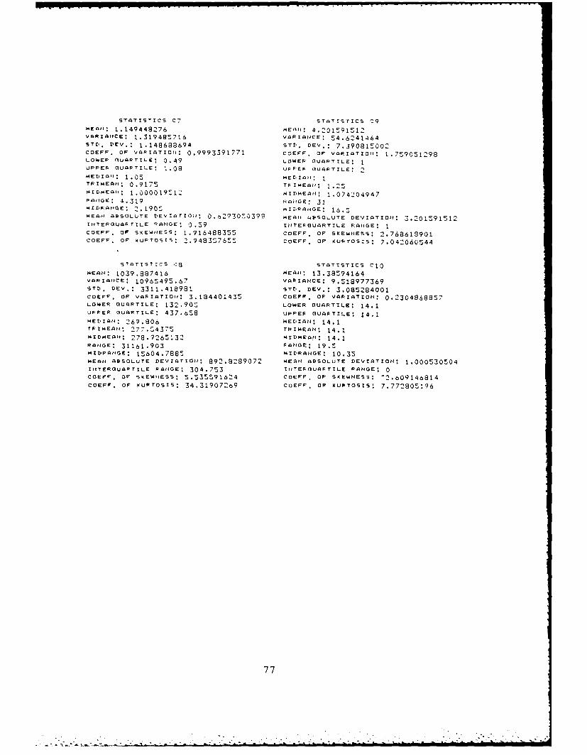
STATISTICS Q7 STATISTICS C9

MEAN : 1.149448276 MEANI 4.201591512VARIANCE: 1.319485716 VARIANCE: 54.6241464

ST,. DEV.: 1.148638694 STD. DEV. : 7.390815002

COEFF. Or VARIATION: 0.9993391771 COEFF, OF VARIATION: 1.759051298LOWER QUARTILE: 0.49 LOWER QUARTILE 1UPPER QUARTILE: 1.08 UFFER aUAFTILE: 2

MEDIAN: 1.05 MEDIA. 1TRIMEA&1 0.9175 TRIMEA;i: 1.25M 1,MEAN: 1..00019512 MIr,,EAN: 1.074204947

RA GE: 4.319 RlGE: 31

MIDRANGE : 2.1905 MIDRANGE: 16.5

MEANf ABSOLUTE DEVIATIO11t 0.629300398 MEAN "I-SOLUTE DEVIATION: 3.201591512

INTER'UAF TILE RANGE ' 0.59 IN.TERQUARTILE RAN4GE: 1

COEFF. OF SKEWNESS: 1.916488355 COEF. OF SKEWNESS: 2.768613901

COEFF, OF MUTOSIS: 2.948357655 coEFP, OF KURTOSIS: 7.042060544

STATISTICS CS STATISTICS CO

MEAN: 1039.387416 MEAN: 13.38594164

vARIA CE: 10965495.67 VARIANCE: 9.518977369

STO. 0Ev.: 3311.418981 ST. 0EV.: 3,085284001

COEFF. OF VARIATION: 3.184401435 COEFF, OF VARIATION: 0.2304868857

LOWER QUARTILE: 132.905 LOWER QUARTILE: 14.1UPPER QUARTILE: 437.658 UPPER QUARTILE: 14.1MEDIAN: 269.806 MEDIAN4: 14.1

TRIMEA 1 277.S4375 TPIMEAN: 14,1

MIDMEAN: 278.9265132 MIDMEAN: 14.1

RANGE : 31161 .903 RANGE: 19.5

MI'RANGE : 15604.7885 MID-,RANGE. 10.35

MEAN ABSOLUTE DEVIATION: 892.8289072 M4EANl ABSOLUTE DEVIATION: 1.000530504

INTErQUARTILE RAIJGE. 304.753 IiJTERPUARTILE RANGE: 0COEFrP OF SKEWNESS: 5.535591624 COEFPF OF SKEWNESS: -2.09146814

COErF. OF KURTOSIS: 34.31907269 COEF. OF KURTOSIS: 7.772805196

77

• . . . . %. -oll,&

LIST OF REFERENCES

1. Naval Coastal Systems Center Techman 4110-1-83, DesignGuidelines for Carbon Dioxide Scrubbers, by M.L. Nuckols,A. Purer, and G.A. Deason, May 1983.

2. Navy Department, U.S. Navy Diving Manual, NAVSEA 0994-LP-001-9010, Washington, D.C., 1978.

3. Navy Experimental Diving Unit Report 3-64, Carbon DioxideAbsorption Systems for SCUBA, by M.W. Goodman, 15 January1965.

4. Navy Experimental Diving Unit Report 1-60, Carbon DioxideAbsorbent Evaluation and Canister Design, by H.W. Husebyand E.J. Michielsen, 6 November 1959.

5. Navy Experimental Diving Unit Report 9-57, Canister DesignCriteria of Carbon Dioxide Removal from SCUBA, by G.J.Duffner, 8 March 1957.

6. The SODASORB Manual of Carbon Dioxide Absorption, W.R.Grace and Co., 1980.

7. A. Purer, G.A. Deason, and M.L. Nuckols, Carbon DioxideAbsorption Characteristics of Hydrated Calcium Hydroxidewith Metal Hydroxide Activators, American Society ofMechanical Engineers, OED-Vol. 10, pp. 57-74, Winter 1982.

8. Shames, I.H., Mechanics of Fluids, pp. 188-204, McGraw-Hill, 1962.

9. Naval Coastal Systems Center TM 368-82, The Effects ofChemical Hydration Level on Carbon Dioxide Absorption byHigh Performance Sodasorb, by M.L. Nuckols, A. Purer,and G.A. Deason, November 1982.

10. Naval Coastal Systems Center TM 364-82, The Effects ofPulsatile Flow on Carbon Dioxide Absorption by HighPerformance Sodasorb, by A. Purer, G. Deason, R. Taylor,M. Nuckols, December 1982.

11. Weisberg, S., Applied Linear Regression, Wiley, 1980.

12. Younger, M.S., A Handbook for Linear Regression,Wadsworth, Inc., 1979.

13. Norusis, M.J., SPSS Introductory Guide: Basic Statisticsand Operations, McGraw Hill, 1982.

78

.......................................... .................

14. Naval Aerospace Medical Research Laboratory, Monograph 17,The Influence of Selected Factors on Shirnkage and Overfitin Multiple Correlation, by N.E. Lane, September 1971.

15. Amick, D.J. and Walberg, H.J., Introductory MultivariateAnalysis, McCutchan, 1975.

16. Mosteller, F. and Tukey, J., Data Analysis and Regression,Addison-Wesley, 1977.

79

. . . . . . . . . . ...... •

INITIAL DISTRIBUTION LIST

No. Copies

1. Defense Technical Information Center 2Cameron StationAlexandria, Virginia 22314

2. Library, Code 0142 2Naval Postgraduate SchoolMonterey, California 93943

3. Professor C.W. Hutchins, Code 55HwDepartment of Operations ResearchNaval Postgraduate SchoolMonterey, California 93943

4. Professor G.F. Lindsay, Code 55LsDepartment of Operations ResearchNaval Postgraduate SchoolMonterey, California 93943

5. Dr. M.L. Nuckols, Code 4110Naval Coastal Systems CenterPanama City, Florida 32407

6. LCDR J.E. Yarborough 22956 Ariane Dr.San Diego, California 92117

80

DTIC