Embed Size (px)
Citation preview

N A S A C O N T R A C T O R
R E P O R T L
LOLN COPY: m m TO
THERMODYNAMIC PROPERTY MEASUREMENTS IN REFLECTED SHOCK AIR PLASMAS AT 12 - 16,OOO"K
by Allen D. Wood and Kenneth H. Wilson
Prepared by LOCKHEED MISSILES & SPACE COMPANY
Palo Alto, Calif. 94304
for Ames Research Center
N A T I O N A L A E R O N A U T I C S A N D S P A C E A D M I N I S T R A T I O N W A S H I N G T O N , D . C. JULY 1970
https://ntrs.nasa.gov/search.jsp?R=19700023343 2018-07-14T20:34:14+00:00Z

- .. .
TECH IJBRARY KAFB, NM
NASA CR-1617
THERMODYNAMIC PROPERTY MEASUREMENTS IN REFLECTED
SHOCK AIR PLASMAS AT 1 2 - 16,000° K
By Allen D. Wood and Kenneth H. Wilson
/ I
P repared under Contract No. NAS 7-704 by LOCKHEED MISSILES & SPACE COMPANY
Palo Alto, Calif. 94304
for Ames Research Center
NATIONAL AERONAUTICS AND SPACE ADMINISTRATION
For sale by the Clearinghouse for Federal Scientif ic and Technical Information Springfield, Virginia 22151 - CFSTI price $3.00
"

.. .
CONTENTS
Page
INTRODUCTION
DESCRIPTION O F APPARATUS AND TECHNIQUE
Spectroscopic Equipment
Photoelectric Technique
Instrument Standardization
Gas Mixing and Tube Loading Procedure
Pressure Measurements
PLASMA THERMOMETRY
Computation of Gasdynamic Properties
Hydrogen Seeding
H - Planck Function Measurement
H Halfwidth Measurement
4955 A Continuum Thermometry
Error Analyses
Use of H Intensities
CY
P o
P RESULTS
Nonsteady Behavior
Results of Temperature Measurements
Intensities of H
Endwall Pressure Results
Incident Shock Velocity Measurement
CONCLUSIONS AND RECOMMENDATIONS
REFERENCES
P
1
4
4 5
7
15
16
19
1 9
2 1
23
25
32
36
42
44
44
47
52
54
54
57
64
ii

. . .
ILLUSTRATIONS
Page Figure
1
2
3
4
1 0
11
1 2
13
14
15
16
1 7
18
19
20
Constant Optical Density Contours From Spectrograms of Standard Lamp 8
Results From Six Attempts To Determine Plasma Intensities by Purely Photographic Methods (Neglecting Reciprocity Effects) 11
Basic Standardization Curve for Wavelengths About H 13 Examples of Endwall Pressure-Time Histories Obtained With Piezotronics Pressure Transducer 18
Operating Region for Best Hydrogen Diagnostics 24
4550- 5100 A Spectrum From Shot 629 (Us = 10.35 mm/psec) 27 4800- 4920 A Spectrum From Shot 619 (Us = 7.97 mm/psec) 30
Data From the H Shape Measurements 31
Comparison of Continuum Predictions From Morris e t Al . and RATRAP Code 33 Continuum Spectral Intensity Predictions at 4955 A for A i r + 10% H2 35
Temperature Sensitivity of Diagnostic Techniques Evaluated Along the Hugoniot States 39
Estimates of Systematic and Random Errors 40
Photoelectric Traces From Shot 630 (Us = 9.51 mm/psec) 45
Time Rate of Temperature Change in Reflected Shock Region 46
Deviations Between Individual Results and Their Mean for Each Shot 49
Deviations Between Gasdynamic and Mean Measured Temperatures 51
Experimental Results and Theoretical Predictions for the Radiation From the Central Region of H 53
Endwall Pressure Results and Incident Shock Velocity Data 55
Experimental Results for the Total Radiant Intensity and Theoretical Predictions Evaluated at Both Gasdynamic and Reduced Conditions 59
Experimental Results for the Radiant Intensity Transmitted by a Quartz Window and Theoretical Predictions Evaluated at Both Gasdynamic and Reduced Conditions 60
P
0
0
P
0
P
iii

Tab le
1
TABLE
Computed Gasdynamic States for the Reflected Shock Region
Page
22
iv

INTRODUCTION
The thermodynamic properties of the plasma formed in the reflected shock region of
a shock tube were measured over a temperature range of 12,000-16,000 OK. These
were diagnostic measurements performed to test the measured temperatures against
the gasdynamic temperatures computed in the conventional manner from the conserva-
tion equations and the equation of state. The results of this effort were essential to
clarify the source of a consistent factor of 2 difference between theoretical predictions
(based on gasdynamic temperatures) and experimental results for the total radiant
intensity of high-temperature air. The total intensity measurements were obtained
over the past several years under prior NASA support and have already been reported. 1
During the preceding contractual year, diagnostic temperature measurements were
made between 10,750 and 13,000 O K using the following spectroscopic techniques: (1) the
integrated line intensity of several NI and 01 lines, (2) the shape of H , H , * and an
NI line, and (3) the spectral intensity of the continuum a t 4935A. The experimental
techniques and results have been described in considerable detail and the salient
features reported in the open l i t e r a t ~ r e . ~ The measured temperatures were limited
to about 13,000 OK because of a rapid loss of accuracy in the results obtained by the
Iirst two techniques. This loss resulted from the rapid rise of the continuum relative
to the spectral intensity .of a line and because the line intensity itself becomes a
slowly varying function of temperature.
a P 0
2
*Hydrogen was present as an impurity in concentrations of a small fraction of 1%.
1
.
Since measurements were desired to at least 16,000"K to cover the range of the total
intensity results, the first task of the present contractual period was to select
thermometric techniques that would not suffer a severe loss of high-temperature
accuracy and that were relatively straightforward and proven. No measurements
involving NI or 01 lines in the visible spectral region were suitable and, of the
techniques employed last year , only the continuum measurement remained. A care-
ful study led to the decision to add a trace species to the nearly pure air plasma for
diagnostic purposes. Hydrogen gas was selected because it is convenient, not unlike
air in a thermodynamic sense, and, most important, because it radiates strongly in
the visible region via the well-known Balmer series l ines.
To avoid reliance on the somewhat uncertain shape2 of the strongest line (Ha) ,
sufficient hydrogen was added to make the well-known second strongest line (H ) P clearly visible above the air continuum so that its shape could be measured. This
required a hydrogen concentration of 10% , but this substantial concentration pro-
vided an additional diagnostic technique - a measurement of the Planck function.
Because the peak spectral absorption coefficient of Ha is about 30 times that of H
a reasonable pathlength could be selected (- 10 cm) wherein Ha was quite optically
thick at its center so that the intensity here was that of the Planck function. At the
same t ime, H was nearly optically thin with the important result that neither
measurement depended strongly on the precise value of the hydrogen concentration.
P '
P
2

The three thermometric techniques used in this work are summarized below:
Diagnostic Technique Advantages Disadvantages
Continuum intensity Almost purely photoelectric; Total reliance on the
at -4955.i high temperature sensitivity work of Morris et al. 4
Shape of H
(4861.33A) function of electron density; photographic techniques; P Shape is a well-documented Requires time-integrated
0
fair temperature sensitivity becomes quite wide
Planck function at Purely photoelectric; yields Low temperature sensi-
Ha (6562.79i) temperature directly; tivity; subject to syste-
requisite radiation constants matic errors
are very well-known
While it is apparent that each of these techniques has disadvantages, they were
believed (and are still believed) to be the best diagnostic techniques for the problem
at hand. The next chapter discusses the special experimental techniques adopted to
minimize these disadvantages while their effect on the accuracy and precision of the
measurements will be assessed in the error analyses in a later chapter.
For this experiment the variables used to specify the thermodynamic state of the
plasma were temperature, pressure, and concentrations (i. e. , mole fractions).
The concentrations were assumed rather than measured since, as will be shown,
they were relatively unimportant. The remaining variable, pressure, was measured
with an endwall pressure gauge in a manner described in the next chapter.
3

,,..,,.-,-. .... .""_....,_.". I"._ ...- ._""
DESCRIPTION OF APPARATUS AND TECHNIQUE
Since much of the apparatus and many of the techniques were similar to those employed
last year,2 the emphasis in this chapter will be on the changes and new techniques.
Spectroscopic Equipment
Two Model 78-000 Jarrell-Ash 1 .5 me te r Wadsworth Spectrographs were employed:
one was used as a conventional spectrograph and the other as a polychromator. The
optical systems were unchanged - both created beams about 1 . 5 mm wide and
10 - 18 mm high across the full diameter of the shock tube. Order-blocking in the
spectrograph was done with a Type I1 UVA Plexiglas f i l ter to clear the f irst order to
above 6700 A, while in the polychromator, suitable Corning Glass color filters were
idaced behind each exit slit. So that both instruments could view the same gas a t
pathlengths less than the full tube diameter, they were located side-by-side on the
same side of the shock tube. The beams were concentric in the shock tube and split
0
by a beam splitter located outside the tube window. The beam splitter was a plain
glass microscope slide, positioned nearly normal to the emergent beam and arranged
so that the transmitted light (- 90%) was sent to the spectrograph with the remainder
sent to the polychromator.
Photomultiplier tubes were placed behind four exit slits in the polychromator. The
exit slits were located as follows:
Main Spectral Feature Center Wavelength (A) Full Width (A) Continuum 4550 19
Central portion of H 4861.3 19
Continuum 5100 19 P
Planck function a t H a 6562.8
4
27

The reasons behind the choice of the widths will be discussed later. Because the red
wing of H extended well over the desired continuum wavelength of 4955 b (this is
9 5 i from H and half-widths of 75 were encountered), the continuum had to be
interpolated from data obtained at 4550 and 5100A where the contribution from H
was small (1 - 9%) and where there was no interference from other lines. The
intensity at the center of H was measured to provide a check on the hydrogen con-
centration and to assist in the interpretation of the photographic spectra.
P
P 0
P
P
- Photoelectric Technique
The entire technique of measuring absolute intensities via calibrated photomultiplier
(PM) tubes was carefully reviewed with the aim of performing these measurements
as accurately as possible. The low temperature sensitivity of the Planck function
and the poor P M tube sensitivity at Ha wavelengths motivated this review.
Two basic considerations were involved: first, the signal/noise ratio of a P M tube
is proportional to the square root of cathode current divided by frequency bandwidth;
and, second, the plasma intensities were up to 10 times the intensity of the tungsten-
ribbon standard lamp used for calibration. Regarding the second point, one can filter
the plasma radiation and/or make the standard lamp appear brighter by opening
entrance and exit slits, replacing the beam splitter with a mir ror , e tc . , o r one can
accept the full magnitude of this disparity. Since filtering the plasma radiation
degrades the signal/noise ratio and since the other operations are difficult to do
reproducibly, it was decided to accept the full disparity. This meant that linearity
was an important consideration. Also the calibration had to be performed under
4
5

near-dc conditions because otherwise the signal/noise ratio would be quite low.
This was done via an in situ calibration with the standard lamp placed inside the shock
tube prior to each shot. The resultant signals were read out on a precision dc micro-
voltmeter.
To ensure that the PM tube response was linear, the following steps were adopted for
the design of each PM tube circuit.
1) The PM tubes were selected for the greatest cathode sensitivity at the
wavelengths involved.
2) Based on manufacturers' information and estimates of the radiative
flux at the exit slits during the experiment (see ref. 2 ) , the gain and dynode
voltage were chosen to cause the peak anode current to be about 20% of the
maximum rating.
3) A dynode resistive divider string was designed which drew at least 10 t imes 4
the steady anode current during the calibration.
4) A tapered set of dynode bypass capacitors, designed to deliver the peak
current for 25 psec with less than a 1% change in dynode voltage, was added
to the divider string.
5) An anode load resistor (1 kQ) was chosen to limit the frequency response to
350 kHz (1 psec rise time) when used with about 15 f t of connecting cable.
TO test the design, each PM tube and circuit was driven to nonlinear behavior
by using a pulsed xenon flashlamp at various distances under nearly the same illumi-
nation (color, cathode area) as in the polychromator. For use in the polychromator ,
the tubes were always operated at an anode current less than 10% of that value where
6
nonlinear behavior was first noted during this test. These nonlinear points were
1 - 2 ma and since these were 2 - 4 times the maximum ratings, it is evident that the
above design criteria are consistent with the test results. During use, the output
levels were never more than a few tenths of a volt.
Three RCA 1P28/1P21 PM tubes were used for the channels at 4550, 4861, and
5100 A. For the Planck function measurement at 6563 A , the flux through the exit
slit was split by a half-silvered mirror and sent to two different P M tubes: one a
DuMont KM2433 with an S-20 response and the other a Hamamatsu R-136 with a
"modifiedff S-10 response. Each of these tubes was powered by a separate John Fluke
power supply so that the precision of the Planck function measurement could be
assessed. A third supply powered the three RCA tubes in parallel.
Instrument Standardization
An accurate measurement of the wide shape of H required that spectral changes in
film sensitivity, instrument transmittance, etc., be taken into account. This procedure
is called instrument standardization and it was made difficult because H is located
in a spectral region where photographic emulsions undergo a rapid change in spectral
sensitivity.
P
P
To illustrate this, Fig. .1 shows several curves of constant optical density obtained
by microdensitometering spectrograms taken of the standard lamp. A s in the poly-
chromator calibration, the standard lamp was placed in the center of the shock tube
and illuminated the spectrograph through the same optics, step wedge, entrance slit,
7

4000 5000 6000 0
WAVELENGTH (A)
7000
Fig. 1 Constant Optical Density Contours From Spectrograms of Standard Lamp
8

etc. , as did the plasma. The exposure times were 0.1 - 0.6 sec and were selected
so that the product of lamp spectral intensity and time ( Iht) was comparable to that
of the plasma with an exposure time of about 20 psec. Typical plasma values are
shown at the position of the exit slits. If viewed upside down, Fig. 1 would resemble
the spectral sensitivity curves supplied by film manufacturers, except that here the
ordinate relates to emission at the source rather than energy density at the film.
The most striking feature of this figure is the rapid change at wavelengths near H
This is caused by the film a s a resul t of the transition between the response of the P '
silver halide on the blue side to that of the sensitizing dye on the red. The films used
in this experiment were Kodak Type I-D Spectroscopic Film for the 3400 - 5800 A
region and Kodak Type 2475 Recording Film for 5800 - 7000 A . The I-D film was
0
chosen because, based on manufacturer's literature, it was supposed to have a fairly
uniform response at H wavelengths. It turned out that this was not so and, in fact,
it was quite comparable to the 2475 film in this respect. It did develop to a high
gamma (large difference in density for small difference in IAt) which facilitated the
photometric process and so w a s useful for this reason. Another feature obtainable
from Fig. 1 is that the curves at different densities are quite similar which implies
that the variations are not particularly density o r intensity-dependent.
P
One measure of the applicability of these curves to the plasma studies is to determine
the reciprocity behavior of the films. This was done by obtaining the spectral inten-
sity of the plasma in two ways. One was by the polychromator measurements dis-
cussed earlier. The other was a purely photographic process involving two films.
The first was known exposure to the standard lamp (- 0.3 sec) and the second a
9

known exposure to the plasma (20 - 30 psec) . Both films were developed simulta-
neously in the same tank to minimize the variables introduced in the development.
Supposedly this left only the reciprocity behavior as the uncontrolled variable. Then
by locating points at the same density and wavelength, the plasma intensity could be
determined by assuming that reciprocity behavior existed. Examples of the ratio of
the polychromatic intensity (averaged over the exposure time) to this purely photo-
graphically determined intensity from six such tests are shown by Fig. 2.
Much can be learned from this figure. First, all the points are below the value of
unity which would be expected in the absence of reciprocity failure. This implies that
reciprocity failure occurred in the 0 . 3 sec standard lamp exposure which is not a t all
unreasonable since this time is quite long for these films (reciprocity law failure
occurs at both very short and very long exposure times). For any one set of points,
the 4550A value is within &lo% of the 4861A value, while the 5100 A value differs 0 0 0
by several times this amount. This is probably because both 4550 and 4861A lie in
the silver halide response while 5100i lies in the dye response. The 4550 - 4861 A points cluster about two different values. While the reason for this is unknown, the
author suspects that the elapsed time before development may be an important factor.
Ordinarily both films were developed shortly after the shot while the standard lamp
exposure was taken at least several hours and sometimes as much as 24 hours prior
to the shot. Unfortunately records of this nature were not maintained.
The conclusion to be drawn from this effort is that reciprocity behavior cannot be
assumed to exist and also that attempting to predict absolute intensities by purely
photographic means is quite uncertain even though good photometric technique is
10

- 8 8 - v
V 8 0
-
0
0 A
0
B 0
0
0
RESULTS INDICATED BY LIKE SYMBOLS OBTAINED FROM THE SAME PAIR OF FILMS
A
"4 0 u3 m *
0 0 rl m
" 4 W
rn W
W u3
b 2 v TYPE I-D FILM 2475 FILM
Fig. 2 Results From Six Attempts To Determine Plasma Intensities by Purely Photographic Methods (Neglecting Reciprocity Effects)
11

practiced. The plasma/standard lamp intensity ratio of l o 4 , o r the exposure time
ratio of , is too great. In retrospect a factor of 10 decrease in the standard
lamp exposure time done, say, by opening the entrance slit lox , may have overcome
much of the reciprocity law failure. However this was not important for this
experiment.
The instrument standardization technique adopted for this experiment embraced the
above observations concerning the film behavior. It avoided any dependence on the
reciprocity law and utilized (but did not depend on) the similarity of the constant-
density curves of Fig. 1. Briefly this technique forced the photographically deter-
mined line shape to fit the polychromatic intensities of 4550 , 4861 , and 5100A and
to follow the trends shown on Fig. 1 at intermediate wavelengths.
0
The process of accomplishing this began with the basic standardization curve shown
by Fig. 3 . The ordinate is called the k-factor defined by:
(Iht) from standard lamp to give a density D at h
(I t) from standard lamp to give same density at 4861A k(h) = _____
0 (1)
h
This basic curve could be obtained from any of the curves of Fig. 1 by dividing by the
appropriate normalizing factor. In fact i t represents an average of several such
curves obtained at densities near unity although the resultant curve is not considered
to be a strong function of density because of the similarity discussed above.
The other important ingredient was the density-log exposure curve (the H-D curve)*
obtained from the actual spectrogram at the brightest spectral feature - the maximum
~
*This curve was obtained from the actual spectrogram through the use of a s tep wedge at the entrance slit of the stigmatic Wadsworth spectrograph. Complete details of this technique are given in Ref. 2.
12

1.5
1.0
0.9
0.8
2 0.7 iz
0.6
0.5
.0.4
0.3
k t (4861.3) = 1.0 + BY
k ' (4550)
4600 4800 5000
WAVELENGTH h (x)
Fig. 3 Basic Standardization Curve for Wavelengths About H P
5200
13

0
of the blue wing of H at 4840 - 50 A . A value of 100% relative exposure was P assigned to this feature following standard photometric technique.2 Again because of
the similarity discussed above, this curve is not considered to be a strong function of
wavelength.
The equation used to obtain the spectral intensity at any wavelength near H was P
The last factor, [ H-D] , refers to the relative exposure at the density of the point of
interest as obtained from the H-D curve in the standard way. The first factor, the
normalizing constant, was obtained by solving the above equation on the average for
the 19 region about 4861.3 corresponding to the H exit slit. Here the k-factor
is about unity with the result that the average value of the last two factors was about
0.90 (the actual shape of H was used here as opposed to the theoretical shape as
discussed later). Then, by inserting the polychromatic intensity on the left-hand
side, the above equation was solved for the normalizing constant [I (H ) I .
P
P
A 0 P
The process of forcing the line shape to fit the polychromatic intensities was accom-
plished by solving Eq. (2) at 4550 and 5100 A for the k' factors. Because these were 0
continuum channels, no averaging was required. These two k f factors generally lay
near, but not upon, the basic standardization curve (Fig. 3) because of the various
approximations involved. The range of these kf values, for all 16 shots of this
experiment,is shown on Fig. 3. The procedure then was to modify this basic curve
by fairing in a smooth curve between the three k t values [kf(H ) = 1 . 0 by definition]
with due regard to the wavelength dependence of the basic curve. The procedure
adopted for this fairing was to make the deviation between these curves linearly
P
14
proportional to the distance away from 4 8 6 1 i . Then Eq. (2) was used with this new 0
k' curve to obtain the entire shape between 4550 and 5100 A. Thus, this standardiza-
tion technique forced the resultant shape to f i t the relatively well-known polychromatic
intensities, utilized the actual H-D curve, and accounted for spectral changes in the
film sensitivity, instrument transmittance, etc., in a realist ic manner.
A somewhat similar procedure was followed for the red region where Ha was located.
Since only one polychromator exit Slit was used, only the normalizing intensity could
be obtained and the standardization curve (derivable from Fig. 1) was used without
any fairing process. This was not a serious disadvantage because, as will be shown
later, the shape of the optically thick Ho line was not essential to this experiment.
Gas Mixing and Tube Loading Procedure
Because of the explosive nature of an air-hydrogen mixture, each mixture was indi-
vidually prepared in a small container by loading from a manifold system connecting
bottles of air and hydrogen. The container was filled to a predetermined total pres-
sure of 45.5 Torr and the contents were then dumped into the evacuated shock tube
with gas flow allowed for 1 min, after which the tube was isolated. The resultant
initial shock tube pressure of 0.206 Torr was measured on several occasions with a
calibrated McLeod gauge (a Todd Scientific Co. Universal Vacuum Gauge).
This calibration was done by admitting known volumes of room air into the evacuated
shock tube and calculating the pressure through Boyle's law and the known tube volume.
These pressures were about 1% above the values measured by a precision manometer
(a Datametrics Inc. Barocel Electronic Manometer) and this agreeement is taken as
verification of the calculated pressure.
15

The calibration revealed that the McLeod gauge read 8% high at pressures about
0.2 Torr, caused at least in par t by an incorrect capillary correction designed into
the instrument scale. This rather significant calibration correction was not dis-
covered until nearly the end of the experimental period during an effort to reconcile
the measured endwall pressures (discussed next) with the gasdynamic pressures.
This report, of course, reflects this correction but since this same gauge was used
to determine initial pressures in the past, the same cannot be said for prior reports
and publications. ” ” The significance of an initial pressure too high by 8% will be
discussed in the appropriate places in this report.
Pressure Measurements
The other measured thermodynamic variable - pressure - was obtained via a pressure
transducer installed flush with the endwall about 38 mm from the tube wall and slightly
outside the field of view of the optical instrumentation.
Two different kinds of pressure transducers were employed during the course of the
experiment. One was a Kistler Instrument Corporation Model 603A (0-3000 psi ,
0.35 pcb/psi, 500 kHz) and the other a pcb Piezotronics, Inc., Model 102A12 (vacuum
to 100 psi , 20 mV/psi, 500 kHz) transducer. Both gauges were calibrated in a special
apparatus which utilized a dynamic process starting with a vacuum.
To demonstrate the nature of the resultant endwall pressure signals, some of the
traces obtained with the pcb Piezotronics gauge are shown on Fig. 4 . Also shown
are the computed gasdynamic pressures, and it is clear that the two values are in good
16

agreement. The results obtained with both transducers, which will be shown later,
indicated that the measured values were within f 3% of the gasdynamic pressure.
The gasdynamic value was used in the thermometric data reduction, and the signifi-
cance of the f 3% uncertainty will be discussed in the error analyses of the next
chapter.

PRESSURE (atm)
A 6 -
SHOT NO. 628 4 - Us = 10.26 mm/ps
2 -
0 -
"-
- TIME
SHOT NO. 630 Us = 9:51 mm/ps
SHOT NO. 631 Uo = 8 . 6 9 mm/ps
1 -
0 - t
k 3 0 -
5 " 4 -
SHOT NO. 633 u0 = 7.93 mm/ps 3 ="- - Pgd
2 -
1 -
0 - -
Fig. 4 Examples of Endwall Pressure-Time Histories Obtained With Piezotronics Pressure Transducer
18

PLASMA THERMOMETRY
Computation of Gasdynamic Properties
The gasdynamic temperatures and pressures provide the basis of comparison through-
out this report and thus it is appropriate to discuss how they were obtained. To begin,
the conservation equations wi l l be written in a simple form without involving the
equation of state.
Applying the equations for conservation of mass, momentum, and energy across the
incident shock wave and eliminating the particle velocity leads to
Since for the conditions of interest the density ratio is about 17 ( i . e . , p2 = 17p1) ,
it is clear that the pressure and enthalpy behind the incident'shock are only weakly
dependent on the density ratio and hence the equation of state.
The result of a similar analysis for the reflected shock is
where
Here density ratios of about 8 ( p , = 8 p ) are typical. While the enthalpy retains its
weak dependence on the density ratio, the pressure does not because of the linear p2
factor. Thus the reflected shock enthalpy is only weakly dependent on the equation of
2 .
state while the reflected shock pressure is linearly dependent on the density p and
hence the equation of state as applied to the gas behind the ineident shock.
2
An equation of state, in the form p = f( P , H ) , w a s obtained from a LMSC free-
energy minimization program called FEMP. FEMP requires thermodynamic data in
the form of curve fits to tabulated values of free energy and entropy for the compo-
nents considered (N2, N , N ,O,O ,H,H , and e - ) . The data for air were taken from
Gilmore and for hydrogen, from McBride. Four sets of curve-fit coefficients were
used to cover the range 6,000 - 18,000"K so that these curve fits would closely
+ + +
5
approximate the tabulated data. To test FEMP, it was run for pure air at near-
gasdynamic conditions of T , P which corresponded to those of the tabulated composi-
tion data by Hilsenrath and B e ~ k e t t . ~ The FEMP values were very close - enthalpy
and density to 0.05% , electron density typically 0.2% with 0.6% maximum, and
individual species concentrations better than the electron concentrations. Although no
composition data were available to check the air f 10% hydrogen mixture, the same
mathematics were employed and there is every reason to believe that the results would
be equally good.
Given elemental composition and temperature and pressure, FEMP can compute the
remaining properties directly, but the gasdynamic variables of enthalpy and pres-
sure require an iterative solution. Since the gasdynamic equations themselves are
implicit in density, a computation of shock states requires a double iteration. The
entire shock calculation program was analyzed and the convergence criteria for
20

densities and enthalpies set at 0. 01% to make the output as good o r better.than the
original thermodynamic data. Table I contains a sampling of the computed gasdy-
namic states for the reflected shock region which cover the range of this experiment.
Besides being used for the gasdynamic calculation, FEMP provided data at "even"
temperatures and pressures for use in calculating the partial derivatives required
in the error analyses which follow, for use in obtaining temperature from electron
density and pressure, and for deriving approximate equations of state.
One practical use of the latter is to consider the effect on the reflected shock tem-
perature if the initial pressure used in the computation was 8% high. From Eqs. (5)
and (6) , i t is clear that 'H would be virtually unchanged and that P would be high
by 8% because of its dependence on p2 . The appropriate form of the equation of
state is T = k(P) O' O4 - O6 (H) - for the conditions of interest . Hence
raising P by 8% would raise the reflected shock temperature by only 0 . 3 - 0. 5%.
5 5
1
To determine the sensitivity of the gasdynamic temperature to the hydrogen concen-
tration, temperatures were computed for various concentrations with P1 and Us
held fixed. The results showed a 60°K decrease in temperature for each 1%
of hydrogen added. Thus a 10% e r r o r in the hydrogen concentration would affect the
gasdynamic temperature by about 0.5% and hence accuracy in the hydrogen concen-
tration was not of paramount importance.
" Hydrogen Seeding
The reasoning behind the decision to seed the plasma with hydrogen has already been
discussed in the Introduction. The experimental requirements for the hydrogen
diagnostic measurements were 1) that H be fairly optically thin and have a peak P
21

:mm/psec:
7 .8
8.0
8.2
8.4
8.6
8.8
9.2
9.6
10.0
10.4
Table 1
COMPUTED GASDYNAMIC STATES FOR THE REFLECTED SHOCK REGION
TI = 294" K Species Mole Fraction Mass Fraction Gram-Atom Ratio PI = 0.206 Torr H1 = 77.9 Cal/g p1 = 2.94-7 g/cc
T5 (" K)
12 , 519
12,910
13,275
13 , 617
13 , 941
14,265
14,829
15,327
15,814
16,335
3.081
3.285
3.490
3.693
3.892
4.082
4.394
4.575
4.766
5.078
H2 0.100 0 ,0077 0.7643 0 2 0.189 0.2311 1,444 N2 0.711 0.7612 5.434
r H5 (cal/g) e
1. 568+4
1. 88+17 1. 6 d 4
1. 52+17
2.68 1.819+4
+17 2.27 1. 734+4 +l7
1. 906+4 3.10 +17
1. 996f4 3.55 +17
2 . 1 7 6 ~ ~
5.79 2. 549+4
4. 38+17
2. 3 d 4 5.08 +17
+17
2. 6. 63+17
N
1. 06+18
1. 04+18
1. 03+18
1 . 0 1 +18
9. $11"~
9.61"~
8. 91+17
7. 99+17
7.11 +17
6.39"'
0
2. 93+17
2. 92+17
2.93 +17
2.90
2.87
+17
+17
2.
2.68 + l 7
2. 46+17
2.25
2.07
+17
+17
Number Densitic
I
H
1.54 + l 7
1. 54+17
1. 54+17
1.52
1.51
1.48
1.41
1.30
1.19
1.10
+l7
+17
"17
+17
+17
+17
+17
!S
, ,
"
1. 20+17
1.
1.49 +17
2.12 +17
2. 46+17
2.
3. 44+17
3. 98+17
4.50
5.12
+17
+l7
1. 99+16
3. o1+I6
2. 48+16
3.57 +16
4.17 +l6
4. 82+16
6.06 +16
7, 20+16 ~ 8. 39+16
+16 9.86
H+
1.13 +16
1.39 +16
1. 68'16
1.98 +16
2.30 +16
2. 64+16
3 . 29+16
3. 86+16
4.46 +16
5. 20+16
N2
7. 45+14
4. 16+14
5. 48+14
3.21 +14
2.52 +14
1. 96'14
1.23 3-14
- -
-
Note: a,bc'ty = a.bc x lo*'.

spectral intensity at least equal to that of the underlying air continuum and 2) that
H be reasonably optically thick over a spectral interval wide enough to permit an
unambiguous measurement of the Planck function. The experimental variables were CY
the amount of hydrogen added and the test gas pathlength. Fortunately, because of
.the nature of the hydrogen lines, all these experimental requirements could be met.
9
This is shown by Fig. 5 which was drawn for the air 4 10% hydrogen mixture. While
a 10% concentration is admittedly a fairly substantial seeding concentration, it is
clear from the figure that this amount was required to keep the H /continuum
intensity ratio above unity at the higher temperatures. The shaded area denotes the P
operating region where E the maximum emissivity at H (peak line + continuum),
is about 0 . 3 while , the maximum emissivity at Ha (considering only the line),
is about 0.999. Pathlengths of 12 and 8. 5 cm were used in this experiment and
the lowest shock velocity was 7.9 mm/psec. A shape measurement is independent
of the absolute intensity provided that the line is optically thin and a peak emissivity
of 0 . 3 is reasonably close to this. For H a , the considerations become more com-
plicated and involve the width of the exit slit.
P ’ P
Ha-Planck Function Measurement
A ra ther wide exit slit was desirable for this measurement for two reasons. First,
the low cathode sensitivity at 6 5 6 3 i of even red-sensitive photomultiplier tubes
dictated that the incident light flux be high to obtain a good signal/noise ratio.
Second, a wide exit slit would minimize a possible correction for boundary layer absorp-
tion at the line center. (There w a s evidence of this on some preliminary spectograms
taken at different conditions and so the Ha shape was monitored during the experiment
for this reason, but no further evidence of boundary layer absorption was found.) On
23

w PI U
H x.
AIR + 10% H2 P = 0.222 torr 1
H CONTINUUM .INTEN d INCIDENT SHOCK VELOCITY, Us (mm/psec)
8 9 10
12,000 13,000 14,000 15.000 16,000 GASDYNAMIC TEMPERATURE, T5 (OK)
Fig. 5 Operating Region for Best Hydrogen Diagnostics
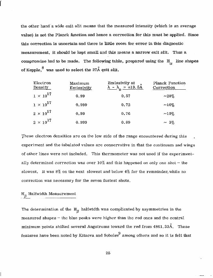
the other hand'a wide exit slit means that the measured intensity (which is an average
value) is not the Planck function and hence a correction for this must be applied. Since
this correction is uncertain and there is little room for e r r o r in this diagnostic
measurement, it should.be kept small and this means a narrow exit slit. Thus a
compromise had to be made. The follopving table, prepared using the Ha line shapes
of Kepple,8 was used to select the 2 7 i exit slit.
Electron Maximum Emissivity at Planck Function Density Emissivity A - h = -+13.5A Correction 0
1 X 0.99 0.57 -20%
1 X 0.999 0.72 -10%
2 x 0.99 0.76 -10%
2 x 0.999 0.89 - 3%
These electron densities are on the low side of the range encountered during this . experiment and the tabulated values are conservative in that the continuum and wings
of other lines were not included. This thermometer was not used if the experiment-
ally determined correction was over 10% and this happened on only one shot - the
slowest. It was 8% on the next slowest and below 4% for the remainder, while no
correction was necessary for the seven fastest shots.
HR Halfwidth Measurement
The determination of the H halfwidth was complicated by asymmetries in the
measured shapes - the blue peaks were higher than the red ones and the central
minimum points shifted several Angstroms toward the red from 4 8 6 1 . 3 3 i . These
features have been noted by Kitaeva and Sobolev among others and so i t is felt that
P
9
25

they are real and not caused by an incorrect instrument standardization process.
Many experimenters symmetrize a measured shape by averaging the two wings, but
this was inconvenient in our case. Attempts to asymmetrize the theoretical shapes
using GriernlkO prescription (Eq. 4-96) were unsuccessful - the correction increased
linearly toward the wings while just the opposite effect appeared warranted.
A practical solution, suggested by H i d l and adopted for this experiment, was to
measure the halfwidths* of the blue and red wings separately, average the results, and
determine the electron density from this average and the halfwidth tabulatiom of
Kepple. This meant abandoning the concept of fitting an entire line shape as employed
last year, but this concept loses significance when unknown asymmetries are
present. In addition, the instrumental halfwidth of 0.29 A was negligibly narrow so no
8
0
computer-aided convolutions were required.
Obtaining the average halfwidth was not without its difficulties as typified by Fig. 6
for the shot with the highest incident shock velocity. This spectrum includes more
than H and the continuum: the ever-present, untabulated NI multiplet at 4630 -
4 6 8 0 i caused little difficulty, but the NI multiplet (4915,4935i ) often lay over the 9
half-intensity point of the red wing. Also both H wings extend over the 4550 and
5 1 0 0 i polychromator channels and complicate the determination of the continuum.
This figure clearly shows the factors influencing the location of these channels to
measure the continuum at 4955 A . To demonstrate the asymmetries , the theoretical
H shape from Kepple at the experimental conditions is superimposed. The under-
prediction of the central minimum point is commonly known and, except for a wave-
length shift, the theoretical shape looks reasonable at the half-intensity points.
P
P
0
8 P
*The halfwidths are defined here ads the intervals between the half optical depth wave- lengths of each wing and 4861.3 A, with each wing treated separately.
26

I
3 X lo4
W x
0
THEORETICAL SHAPE O F Hp AT MEASURED CONDITIONS
-MEASURED
\
CONTINUUM - '"' POSITION OF' POLYCHROMATOR
H
EXIT SLITS
4l- 5100
I I I I I I I I I I I I 4600 4700 4800 4900 5000 5100
WAVELENGTH, h (i)
0
Fig. 6 4550- 5100 A Spectrum From Shot 629 (U = 10.35 mm/psec) S

, -. ._ . .. .. . . . . ... . - . ..
The data reduction procedure used to measure the halfwidths was iterative, but an
educated initial guess of the temperature and the corresponding (see below) electron
density minimized this problem. Because the measured spectrum was on an absolute
basis, the contribution of the NI multiplet could be determined and subtracted off.
This was at most a 7% correction since the multiplet peaks were avoided. The con-
9
tinuum levels at 4550 and 5100 A were determined by subtracting off the wings of H
obtained from either the tabulated shape or , at lower electron densities, the asymptotic
wing formula also tabulated by Kepple. Since this wing correction depended on the
height of H which in turn depended on the continuum level, a secondary iteration was
required. This was done carefully since it affected the continuum level which was
important in its own right. This was at most a 9% correction, but it was never less
than 1% because the wings extend quite far and the relative height of H increased at
lower temperatures. (See Fig. 5. ) Both this and the N19 correction were facilitated
by the advance preparation.of curves for the NI multiplet intensity at various wave-
lengths and the H wing.at 4550 and 5 1 0 0 i evaluated along the Hugoniot states.
P
P
P
9
P
The red and blue halfwidths were then measured relative to ho = 4861.3 A which is
unimportant if they are averaged, but later their ratio will be used to estimate the
experimental precision. Since peak emissivities of about 0.35 were encountered,
opacity effects were taken into account by measuring the halfwidths at the half-
optical depth points rather than the half-intensity points. This was done by converting
the peak and continuum intensities into optical depths, calculating the half-optical
depths, and converting these back into intensities which were then plotted on the
spectrum as shown. These differ in Fig. 6 because the blue peak and the blue
28
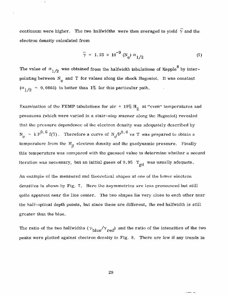
continuum were higher. The two halfwidths were then averaged to yield 7 and the
electron density calculated from
The value of a! was obtained from the halfwidth tabulations of Kepple by inter-
polating between Ne and T for values along the shock Hugoniot. It was constant
8 1 /2
(a! 1/2 = 0.0865) to better than 1% for this particular path.
Examination of the FEMP tabulations for air + 10% H2 at f'evenf' temperatures and
pressures (which were varied in a stair-step manner along the Hugoniot) revealed
that the pressure dependence of the electron density was adequately described by
Ne = k Po. f(T) . Therefore a curve of N k p o * vs T was prepared to obtain a
temperature from the H electron density and the gasdynamic pressure. Finally
this temperature was compared with the guessed value to determine whether a second
iteration was necessary, but an initial guess of 0.95 T was usually adequate.
P
gd
An example of the measured and theoretical shapes at one of the lower electron
densities is shown by Fig. 7. Here the asymmetries are l e s s pronounced but still
quite apparent near the line center. The two shapes lie very close to each other near
the half-optical depth points, but since these are different, the red halfwidth is still
greater than the blue.
The ratio of the two halfwidths ( yblue/y ) and the ratio of the intensities of the two red
peaks were plotted against electron density in Fig. 8. There are few if any trends in
29

0 w
1 . 2 A
F k m I 4 E. 1.ox 10
\ 0
5 H x 0.8
i5 E! 0.6 z H 4 Pi
0.4
k
MEASURED SPECTRUM -
-
-
-
N = 1.66 X 10
b PI 0.2 w m 1 """"""""""_ """"_" "" "__
CONTINUUM
0 1 I 1 I I I I I I I I 4800 4850 49 00
WAVELENGTH, h (A)
0
Fig, 7 4800- 4920 A Spectrum From Shot 619 (U = 7.97 mm/psec) S

0 0
1.0
+ +
0.80' I I I I
8 1.00 E A
A A A A 2 - l A A A A A c13 2 0.90-
A A A
P a
c13O LIE
8 2 0.80 I I I I
B A E o 1 x 2 x 3 x 10 4 x log7 5 x
17
MEASURED ELECTRON DENSITY
Fig, 8 Data From the H Shape Measurements P
c
these ratios, so the fact that the halfwidth ratios vary by & 7% provides an estimate
of the experimental precision in this measurement. The lower curve of Fig. 8 repre-
sents the ratio of the average spectral intensity of H over the 19 exit slit width
to the average peak spectral intensity of the line. This ratio will be used in a la te r
section where a theoretical prediction of the H radiation is made.
P
P
4955 i Continuum Thermometry
The experimental value for the spectral intensity of the continuum at 4955 A was
obtained by linear interpolation between the 4550 and 5100 A values obtained from the 0
polychromator after subtraction of the H wings as explained in the preceding section. P This was a small correction - between 1 and 9% of the polychromatic intensities.
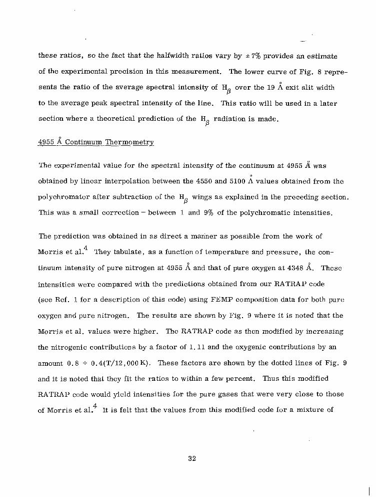
The prediction was obtained in as direct a manner as possible from the work of
Morr is e t al! They tabulate, as a function of temperature and pressure, the con-
tinuum intensity of pure nitrogen at 4955 i and that of pure oxygen at 4348 i, These
intensities were compared with the predictions obtained from our RATRAP code
(see Ref. 1 for a description of this code) using FEMP composition data for both pure
oxygen and pure nitrogen. The results are shown by Fig. 9 where it is noted that the
Morr i s e t al. values were higher. The RATRAP code as then modified by increasing
the nitrogenic contributions by a factor of 1.11 and the oxygenic contributions by an
amount 0.8 + 0.4(T/12,000 K). These factors are shown by the dotted lines of Fig. 9
and it is noted that they fit the ratios to within a few percent. Thus this modified
RATRAP code would yield intensities for the pure gases that were very close to those
of Morr is e t a1.4 It is felt that the values from this modified code for a mixture of
32

w w
1.5
1 .3
1 . 2
1.1
1.0
OXYGEN
V 5 atm atm 1 4348 V
NITROGEN 0' 0
5 atm /' ,HO 0
0' 0 KO= 0.8 $. 0.4 (T/12,000)
\
0
V eo 0
0
0'
V N0
0
0' 0
v KN = 1.1 1
6 v "g """"""""""" -
e - .
7-
m a
io, ooo 12,000 14,000 16,000 18,000 TEMPEFUTURE ( O K )
Fig. 9 Comparison of Continuum Predictions From Morris et Al. and Ratrap Code

these two gases at the wavelength of the principal constituent represent a reasonable
application of their work. While this modification procedure did not involve the
RATRAP predictions for pure hydrogen, its continuum is relatively weak and since
the plasma contains only 10% hydrogen, possible errors f rom this source would have
to be quite small.
Therefore the continuum spectral intensity predictions for air + 10% hydrogen at
4955 A were obtained from this modified RATRAP code and the appropriate FEMP
composition data. The results were scaled by (P)'. and are shown for the two path-
0
lengths of this experiment in Fig. 10 where the validity of this scaling can be assessed.
To justify that no large errors were made in this procedure, it is noted that the lower
solid curve is within f 3% of the Morris et a1 . values for pure nitrogen at 5 atm when 4
their tabulated values are multiplied by 8.5 (an optically thin pathlength) , divided by
8 . 1 (the 5-atm pressure scaling), and then multiplied by 0.80. This last factor was
obtained from the mole-fractions of the test gas by assuming that oxygen radiates half
as much as nitrogen, and hydrogen negligibly little - a rough but not unreasonable
approximation to locate large errors.
The error analysis to be considered in the next section will require an estimate of the
accuracy of the curves of Fig. 10. For plasma thermometry, the continuum intensity
can be considered as the means of transferring the plasma temperature diagnostic work
of Morr is e t aL on their arcs to our plasmas. In this sense the validity of the con-
tinuum cross sections and attachment energies they obtained is of secondary import-
ance because their conditions (9 - 14,000°K, 1 - 2 atm) are close to ours. They
determined their arc temperatures by measuring the integrated line intensity of well-
4
34

3 x 10:
1 o3
1 o2
40
12 cm PATHLENGTH 5 atm
8.5 cm PATHLENGTH 5 atm
Fig.
TEMPERATURE ( O K )
0
10 Continuum Spectral Intensity Predictions at 4955 A for Air + 10% H2
35

known M and 01 lines. Assuming a f 5% measurement using f 10% f-numbers and
an accurate pressure, it can be shown that this technique is capable of yielding better
than f 1.5% temperatures for pure gases at their conditions. Actually their arcs were
nonisothermal and their test gases not pure, but these are largely random effects which
are of small consequence since they made repetitive measurements. Because they
measured the continuum intensity with the same spectroscopic system at an adjacent
wavelength, this better than 1.5% temperature uncertainty is equivalent to a f 15%
uncertainty in their tabulated values for the continuum intensity. The process of
computing the curves of Fig. 10 included the effects of the imperfections in the
modified RATRAP procedure, the wavelength change for oxygen, and the untested
hydrogen contribution. These are estimated to be f 5% and, in view of the symmetrical
nature of the corrections shown in Fig. 9 and the close correspondence with the rough
approximation made above, this wi l l be treated as a random error. Thus, for use in
the following error analysis, the curves of Fig. 10 are estimated to have f 15%
systematic errors and * 5% random e r ro r s .
2
Error Analyses
In all three diagnostic techniques, a temperature was obtained from the measurement
of a radiative quantity M which depended on the thermodynamic state and certain
physical constants C . The functional relationship is M = f (T , P , C) and the total
differential of M can be cast in the following form:
36

The left side represents the temperature uncertainty while the numerator on the
right includes the uncertainty in the measurement of M together with the effect of an
uncertain pressure and physical constants. During the following analyses, those
portions of the numerator which represent possible systematic errors affecting the
accuracy of the measurements will be separated from the random errors which
affect the precision. This numerator is divided by the dimensionless partial derivative
which is called the temperature sensitivity.
The measurement of the Planck function Bh a t the Ha! wavelength is easily analyzed
because it is not pressure dependent and the radiation constants may be considered as
accurately known. Thus, for the Planck
5 D
function, Eq. (8) becomes
denominator
where C2 = 1.439 x 10 pK and, for Ha, , h = 0 . 6 5 6 3 ~ . The systematic errors
are entirely those of the standard lamp - the calibration supplied with the lamp is
stated by the manufacturer to be accurate to * 2% and this was increased to + 3% by
the adoption of an often-compared working standard. The random errors, introduced
by meter and oscilloscope calibrations, PM tube dynode voltage changes, etc. , may
be estimated by noting that the ratio of the two 6563 A intensities varied between 0.96
and 1.08 during the course of this experiment. Since the two red P M tubes were
operated completely independently and since their outputs were averaged to obtain a
4
0
single intensity, the random error in the Ha, intensity is estimated to be &3%. The
. correction for the nonblack regions near the slit edges was less than 10% of this
37

intensity and assuming that the correction was accurate to f 10% adds another f 1% to
the random error. Thus the random errors are estimated to be &4%. The tempera-
ture sensitivity of Eq. (9) is evaluated in Fig. 11 and the resultant estimates of the
systematic and random errors are shown in Figs. 12-A and 12-B, respectively.
For the measurement of the 4955 k continuum intensity IAc , Eq. (8) becomes
dIAc d P dC 1 . 3 - " P C "
denominator
' P
where the coefficient of the pressure uncertainty was obtained from the scaling used
in Fig. 10. The systematic errors of f 18% stem from the f 15% estimate of the
accuracy of the curves of Fig. 10 as discussed in the previous section together with
the &3% accuracy of the working standard lamp as discussed above.
During the course of the experiment, the ratio of the corrected polychromatic conti-
nuum intensities at 4550 A to those at 5100 A varied between 1 . 0 2 and 1.16. (The 0 0
extremes occurred at nearly the same plasma temperature. ) Incidentally the modi-
fied RATRAP code predictions yielded ratios of 1 .12 - 1.18 and, while not to be
taken literally, are regarded as encouraging evidence that no gross errors were
present. The linear interpolation to 4955 A was essentially an averaging process 0
leading to an estimate of f 4% for this value. The less-than-l0Y 0 Hp wing
corrections, if done to only A 1076, contribute another f 1%. The rt 3% pressure
uncertainty contributes f 4% and the random errors associated with the computation
of the curves of Fig. 10 were estimated to be f 5%. Thus, the total random errors
are estimated to be * 14%.
38

10
8
6
4
2
0
M = 4955 dl CONTINUUM INTENSITY
1 1 ) O O O 12) 000 13,000 14) 000
TEMPERATURE (OK) 15) 000 16,000
Fig. 11 Temperature Sensitivity of Diagnostic Techniques Evaluated Along the Hugoniot States

. . ... . . . . . . -. . . .”.
&5
- 4 -
0
4955 A CONTINUUM E /
/ /
E+
ffi
3 -
”””
.A’
a ///-
//
,I’ 5 HALFWIDTH ”” -/ P
g 2 - ””- #””
/ ””
ffi w 1 - PLANCK FUNCTION
0 I I I I I I I
TEMPERATURE (OK) 12,000 14,000 16,000
A. Systematic Errors
H HALFWIDTH / P
0/4 49556; CONTINUUM le
a / /’ / ”
$ 2 ””” ””- ”” PLANCK FUNCTION 0 P; e”-” ”-”
I I I I I I I 12,000 14,000 16,000
TEMPERATURE (OK)
B. Random Errors
Fig. 12 Estimates of Systematic and Random E r r o r s
40

The temperature sensitivity shown in Fig. 11 was obtained by numerical differentiation
of the modified RATRAP code predictions and the resultant e r ror es t imates are shown
in Fig. 12 .
For the H shape measurement, the measured quantity was the averaged halfwidth
y given by Eq. (7) and temperature is introduced by the discussion of the electron
density that followed. Thus Eq. (8) becomes
P -
denominator
The systematic errors lie entirely in the validity of the constant (Y since it is not
felt that our treatment of the asymmetries was significantly different from anyone
else 's . Kepple reports that his H shapes (i. e . , halfwidths) agree with experimental
measurements to *4% over electron densities of 2 x - 2 x and
20,000"K. However Shumaker and Popenoe12 assert that only limited experimental
tests have been performed above 8 x cm-3 and claim, on the basis of their
work, that Kepple's widths are too wide by 7% at 2 x lOI7 ~ m - ~ . In a s imilar
experiment, Morris and Kreyl' report' that Kepple's widths are too wide by 3 - 5%
although they do not regard this as significant. Therefore a systematic uncertainty
of *6% is assigned to Kepple's value of a and we note here for use later that the
-6% extreme might be more nearly the true value, at least at electron densities
near 2 x 10 .
1/2
8 P
1/2
17
The random errors include the %7% halfwidth measurement discussed earlier while
the 53% pressure uncertainty contributes another + l%,making the total random
41

e r r o r s f 8%. The temperature sensitivity was obtained from the FEMP tabulations
and is plotted in Fig. 11; the resultant error estimates are plotted in Fig. 12.
The validity of all these error estimates wi l l be assessed in the next chapter when the
individual measurements are discussed.
Use of HR Intensities
0
The measured intensity of the 19 A central portion of H was not used as a pr imary
diagnostic technique because it would not be in the same accuracy class as the three P
just discussed. Thermometry on a portion of a line shape is basically undesirable
because it combines the uncertainties of both intensities and shapes and this is not
compensated by an increase in the temperature sensitivity. Further,for H the
theoretical shape near the center is none too good (although experimental shapes are P
available). Finally in the case at hand, the intensity directly involves the hydrogen
number density - a dependence avoided in the shape of H and the intensity of
optically thick H a . P
The H intensities were used to determine the nonsteady behavior'and as a measure
of the experimental concentration of hydrogen as discussed in the next chapter.
Assuming (for simplicity only) that the H radiation was optically thin, the spectral P intensity for a pathlength of 6 (cm) is
P
where S ( a ) is normally the shape parameter tabulated by Kepple . However, for the
problem at hand, this shape did not adequately represent the central portion of the line
shape as indicated earlier by Figs. 6 and 7. Therefore, to represent the average
8
42

0
spectral intensity over the 19 A exit slit, $(a ) was taken to be the peak tabulated
value multiplied by the experimentally obtained ratio S((Y )/S( (Y )max plotted in Fig. 8.
This procedure w a s not strictly correct because the resultant hybrid shape was no
longer normalized to unity, but the errors incurred were small because the central
portion was a small fraction of the total shape and the theoretical shapes appeared to
reasonably represent the experimental shapes from the maximum points out toward
the wings. The temperature sensitivity of this intensity is given by
" T "A I - - " T aNHl 2 T aNel 1 2 . 8
IA aT P -" -
NH aT P 3 Ne i3T kT + -
and is plotted in Fig. 11.
43

RESULTS
Nonsteady Behavior
The photoelectric traces from the polychromator and the zero-order trace from the
spectrograph again2 showed the marked similarity which was taken as experimental
verification of the presence of chemical equilibrium. These traces did, however,
generally show a linear decrease with time indicative of unsteady behavior. This is
typified by Fig. 13 where it is apparent that the continuum channels decreased the
most and the Planck function the least. However this is entirely consistent with the
temperature sensitivities of these radiative quantities. (See Fig. 11.)
These decreases were systematized by dividing each slope (% change in M p e r unit
time) by the appropriate temperature sensitivity (% change in M per % change in T)
to yield the rate of temperature change. The results for all the traces obtained dur-
ing this experiment are shown in Fig. 14. The two continuum and the two Planck
function traces were each averaged - they did not differ substantially. The traces
were linearized to the point where an obvious bump or dip signified the end of the
test time. The temperature Sensitivity of the H channel was appropriately weighted
for the underlying continuum. P
The most remarkable feature of Fig. 14 is the utter lack of any temperature depen-
dence. This was entirely unexpected and must be taken as strong evidence that the
temperature changes were not caused by radiative cooling because this would be
strongly temperature dependent.
44
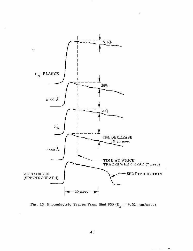
I
28% DECREASE
TIME AT WHICH TRACES WERE R.EAD (7 psec)
ZERO ORDER SHUTTER ACTION
Fig. 13 Photoelectric Traces From Shot 630 (Us = 9.51 mm/psec)
45

a w
Fr 0 w E
P$ 4 -0.4
O HB A CONTINUUM
0 PLANCK
B """"""""" """""""""""""
bo -0
5%" f i 8 w 0 0 0 0 a6 j8 @
.
-
+ . c
-
- -
12,000 13,000 14,000 15,000 16,000 I I I I I 1 I I
I I I I 7 . 5 8 8 . 5 9 9 . 5 10 10.5
GASDYNAMIC TEMPERATURE, T, ( O K )
INCIDENT SHOCK VELOCITY, Us (mm/psec)
Fig. 14 Time Rate of Temperature Change in Reflected Shock Region

From a thermometric standpoint the small magnitude of the ordinate is noteworthy.
The data points average at a value of about -O.l%/psec corresponding to a relatively
small 1% decrease in temperature over 10 psec. The rate derived from the Planck
junction is lowest on all but two shots (where it is close) while the H and continuum-
derived rates tend to be quite similar. This is consistent with the experimental con-
ditons. The large optical depth at Ha! made the Planck function sensitive to sidewall
boundary layers while the optically thin conditions at H and especially the con-
tinuum made these measurements reflect bulk gas properties over the full 8.5- or
12-cm pathlength. The fact that these rates are as close as they a r e is important
evidence that no appreciable absorption occurred in the sidewall boundary layer.
P
P
Since time-dependent changes were observed, it is appropriate to comment on where
(in time) the results were based. The polychromatic traces were read about 7 psec
after passage of the reflected shock to correspond to an average over the 15 psec
measurement time in the cavity model used to obtain the total intensity results.
The exposure times in the spectrograph averaged about 22 psec (min. 14, max. 28)
and thus the H shapes represented a somewhat longer time-average than did the
purely photoelectric measurements of the Planck function and the continuum intensity.
However in light of the results of Fig. 14, the difference in temperature was negligibly
small and no adjustment was made.
1
P
- Results -. - " of - Tern-erature Measurements
The first task of this section is to assess the quality of the results. The basis is the
average of the three (only two in several cases) results from the three different
thermometric techniques employed on each shot. The percentage deviations between
47

each result and this mean value are shown by Fig. 15. To assist this assessment,
e r r o r bands representing the average of the systematic error estimates (Fig. 12-A)
were also drawn.
Taken by themselves, the data scatter by less than -+3% which is testimony to the
quality of the results. It is interesting to note that the error estimates (Fig. 12)
would allow the data scatter to increase at the higher temperatures, but that such
behavior was not realized in practice. While some systematic deviations are apparent,
this behavior is largely within the limits of the error bands - the low-temperature H
results being a possible exception. The two experiments which reported the halfwidths P
to be about 6% too wide12 ' l3 were conducted at electron densities corresponding to
about 13,000" K in Fig. 15. The temperature sensitivity here is about 4 so reducing
Kepple's values by 6% would raise the H temperatures 1.5% and make the agree- P ment here look better. However this same correction, if applied uniformly, would
raise the H results 3% at the high-temperature end and here they look good as they
are . Since such a correction would represent an extrapolation to much higher electron
densities where no similar data are available, it was decided to use Kepple's values
uniformly.
8
P
8
Such comments notwithstanding, the average systematic error bands enclose the
majority of the data points and those outside are no farther than (and in most cases
considerably within) the deviations allowed by the random error es t imates of
Fig. 12-B. Therefore these bands represent a liberal estimate of the accuracy of
this experiment. In the figure to follow, the error bars represent the appropriate
height of these bands. The plotted point - the mean measured temperature - represents
48

$I ' I 3 E HP A CONTINUUM
0 PLANCK
' 0
0 A 0 0
A
"""- br-" -""""" a- ",.d"d" -7 A AVERAGE
-2
0 0 A 0 SYSTEMATIC A O L Q
A ERROR
v-o"" I - 0 "" ~ ~ ~ ~ ~ ~ ~ ~ ~ - ~ ~ - ~ oA ? F A
Q""" --"""- -" -5
A 0 A 0 A 0 """
0 "
0 0 0 " 0 "
0 0
I- o -4
-6 + 1 I I 1 I
12,000 13,000 14,000 15,000 16,000
MEAN MEASURED TEMPERATURE, TM ( O K )
Fig. 15 Deviations Between Individual Results and Their Mean for Each Shot

the most probable value because the systematic errors in each technique stem from
largely unrelated sources.
The principal objective of this research was to compare the measured temperatures
with the gasdynamic temperatures and this comparison is presented by Fig. 16.
Also included are the results obtained last year2 ' with * 2% e r r o r b a r s obtained by
considerations similar to those above and with the deviations reduced by subtracting
0.35% to compensate for the lower initial pressure caused by the McLeod gauge cali-
bration correction. Thus Fig. 16 contains all the thermometric results obtained
during the whole research effort.
It is clear from Fig. 16 that the gasdynamic temperature w a s not realized on the
bulk of the shots. Last year2 ' it was remarked that the shock tube operation was
e r ra t ic - shots with comparable incident shock speeds yielded measured tempera-
tures that differed by almost 1000°K. To a lesser extent, this behavior persisted
over the 12 - 14,000"K range while for the eight shots above 14,00O0K, the shock tube
acted quite repeatably and here regular deviations of 5 - 6% were encountered.
It is unfortunate that the shock tube did not behave more regularly so that the total
radiation datal could be compared more accurately. Taken alone, the results from
this year would appear to show a trend but this disappears when balanced against the
earlier results. There is no reason to discount these earlier results which, in fact,
represent averages of seven measurements employing three different techniques.
Since a temperature-dependent trend would be expected if radiative cooling were the
loss mechanism, the lack of such a trend in the results of Fig. 16 would indicate that
50

0
-2
-4
-6
-8
-10
- T 0 THIS WORK
1
11,000 12,000 13,000 14,000 15 , 000 16,000 MEAN MEASURED TEMPERATURE, TM ( O K )
Fig. 16 Deviations Between Gasdynamic and Mean Measured Temperatures

radiative cooling was unimportant. This supports the conclusion derived from the
rates of Fig. 14 where time-dependent changes and not absolute values were
important.
Intensities of HB
0
Figure 17 shows the polychromatic intensities for the 19 A central portion of H
obtained upon subtraction of the continuum level as determined by the 4550 and 5 1 0 0 i
channels with opacity effects taken into account. Also shown are theoretical curves
evaluated at both gasdynamic conditions (see Table 1) and at the same pressures but
with temperatures reduced 5% below the gasdynamic values. These curves were
obtained from a relation similar to Eq. (12) but with opacity effects included.
P
These curves are not intended to be used as primary thermometers - if they were,
they would indicate temperatures 1. 5 - 3% above those of Fig. 16. The intensity of
H would make a relatively poor thermometer for reasons discussed earlier. Rather
the curves should be considered as indication of a 10% systematic error which might
well have been caused by the presence of 11% hydrogen rather than the assumed 1 0 % .
In retrospect this is not unreasonable since the hydrogen gas was admitted to the
mixing container first and thorough mixing may not have occurred. Since neither the
other hydrogen-derived diagnostics nor the gasdynamic temperatures depend strongly
on the hydrogen concentration, an 11% hydrogen concentration would have very little
effect on the results of this experiment.
P
52

2 x 10
1 o4
PATHLENGTH = 8.5 cm / /
/ /
THEORY EVALUATED AT GASDYNAMIC CONDITIONS
10% THEORY WITH TEMPERATURES REDUCED 5%
0 EXPERIMENTAL DATA POINTS CORRECTED (IF NECESSARY) TO AN 8.5 cm PATHLENGTH
7.5 8 8.5 9 9.5 10 10.5
INCIDENT SHOCK VELOCITY, Us (mm/psec)
Fig. 17 Exper imen ta l Resu l t s and Theore t i ca l P red ic t ions fo r t he Rad ia t ion From the Central Region of HP
53

Endwall Pressure Resul ts
Usable endwall pressures were obtained on 10 of the 16 shots and the results are
shown in Fig. 18-A. The e r ror bars represent the confidence level of each trans-
ducer and include uncertainties in both the calibration and the reading of the actual
t races . It is clear from this figure that the measured values were within *3% of
the gasdynamic pressures. The symmetrical nature of the data scatter precludes
any systematic errors and little, if any, significance should be attached to the *3%
scatter because of the difficulty in reading the gauge traces (see Fig. 4) with any I L
greater precision. The error analyses of the preceding chapter showed that this
small scatter did not appreciably affect the precision of the measured temperatures.
Incident Shock Velocity Measurement
This velocity was determined from time intervals measured between three ionization-
type probes located 1 f t apart near the endwall as shown by Fig. 18-B. The
outputs from adjacent probes were displayed as A minus B signals on oscilloscopes
whose sweeps were calibrated by superimposing a 1-MHz sine wave from a crystal
oscillator on the resultant oscillogram. The same operational mode was used -
single sweep after a long wait. The time intervals were 30 - 40 p e c and estimating
that they could be read to the nearest 1/4 cycle of the sine wave yields an accuracy
estimate of + 0.4% for the shock velocity. The two values so obtained were averaged
to provide the basis for the gasdynamic properties used throughout this report.
To make certain that these time intervals were meaningful, several experiments have
been performed in the past. These involved installing pressure gauges either in place
54

0 -KISTLER GAUGE
INCIDENT SHOCK VELOCITY, Us (mm/psec)
A. Results of Endwall Pressure Measurement
SIGNIFICANT SHOCK POSITION
NO. 1 NO. 2 NO. 3
I 1 L 1 I DISTANCE FROM 6 67 4;2 767 a i 5 ENDWALL (mm)
B. Location of Ionization Probes
h
‘ 2 t-z 5 0 0 r(
X 1 + cr)
0 tp
Fl -1
-2 8 9 10
INCIDENT SHOCK VELOCITY, Us (mm/psec)
C. Incident Shock Velocity Change Near Endwall
Fig. 18 Endwall Pressure Results and Incident Shock Velocity Data
55
of o r in addition to the ionization probes. The results have always indicated that the
time intervals obtained from the ionization probes adequately represented those of the
passage of the gasdynamic shock front.
The average velocity used for gasdynamic purposes represents the velocity at probe
No. 2. The difference between the two velocities actually measured represents the
change in a 1-ft interval and these differences are plotted in Fig. 18-C with + 0.8%
e r r o r b a r s to indicate the error doubling when differences are used, It is clear from
this figure that the shock accelerated on about 3/4 of the shots and, for discussion
purposes, the average change was an acceleration of about 0.6%/ft.
The overall density ratio (p5/p1) was about 125. (See Table 1.) Thus the test gas
7 mm from the endwall (where temperatures were measured) was processed by the
incident shock when it was about 875 mm from the endwall - a location about 1 .5 f t
farther upstream than probe No. 2. The velocities at this point were, on the average,
about 1% l e s s than those at probe No. 2. It may be argued that the velocities at this
upstream location would have been a more significant basis for the gasdynamic
properties. This would lower the gasdynamic temperatures by 1 . 9 % at 11,00O"K,
1 .2% a t 13,00O"K, and 0.8% at 15,000"K and hence reduce the deviations shown in
Fig. 16 by these amounts. An effort was made to determine i f a shot-by-shot
correlation existed between the results of Fig. 16 and an individually applied correc-
tion for the shock speed. None could be determined since the corrections for the
large-deviation points were about equally distributed between upward and downward
revisions.
56

CONCLUSIONS AND RECOMMENDATIONS
This experiment successfully measured the thermodynamic properties of the test gas
for temperatures up to nearly 16,000"K. The measured temperatures were about 5%
below the gasdynamic values at temperatures above 13,000"K and varied erratically
between 0 and 6- 8% below at lower temperatures. No explanation was found for
this erratic behavior. The accuracy of these measurements was about f 2% as
predicted by the error analyses and as realized in the agreement obtained between
measurements involving three different thermometric techniques. The endwall
pressures were within + 3% of the gasdynamic pressures.
No significant evidence of radiative cooling w a s found since no temperature-dependent
trends were evident in either the rates at which the test gas temperatures decreased
or in the deviations between the measured and gasdynamic temperatures. No
appreciable absorption occurred in the sidewall boundary layer since the optically
thick Planck function rates and temperatures agreed with the results obtained from
the other two diagnostic techniques at nearly optically thin conditions.
It may well be that the observed deviations from ideal shock tube behavioq represent
the total of many small effects. Three were found during this work. One, the shock
accelerations, could lower the gasdynamic temperatures about 1% if the upstream
shock velocity were used. Another was the less-than-l% increase in the measured
temperatures that could be gained by correcting the measured temperatures for the
observed rates of decrease. A third, caused by the apparent presence of an 11%
hydrogen concentration rather than the assumed lo%, would lower the gasdynamic
57

temperatures by about 0.5%. Taken together, these three effects add to about 2% which
leaves unexplained the largest par t of the observed deviations from the gasdynamic
temperatures. There may be other effects, although none were evident during this
research.
Whatever the cause or causes of the observed behavior, the measured temperatures
were obtained in a manner corresponding to the way in which the integrated intensity
measurements were made several years ago: Therefore the results of this experi-
ment as shown by Fig. 16 may be applied directly to these measurements and this
was the ultimate purpose of this research effort.
The results of the integrated intensity measurements a r e shown in Figs. 1 9 and 20.
They were taken directly from a previous report and, except for the theoretical
predictions, the figures are identical. The predictions were obtained from a current
RATRAP code which yields values that are somewhat lower than those from the version
used previously. Besides several minor computational improvements, the major
changes in the current code were the correction of a numerical error in the ionization
potentials of NI and 01 and a limiting of the effective shifts of the photoionization edges
to 0 . 2 eV. Previously the shifts exceeded this value at high electron densities and this
meant that the contribution from high-lying visible-LR lines was included twice. These
changes result in predictions that are 15- 20% lower in the window spectral region and
10- 20% lower for the total spectrum.
1
In addition, the 8% calibration correction for the McLeod gage used to determine the
initial tube pressure, which was only recently discovered, lowered the pressure used
58

REDUCED TEMPERATURE (OK) 10,000 12,000 14,000 -1". ~. I- t I -~ ~ ~ ~
- 1 I I I I I
I 10,000 12 , 000 14,000 16,000
GASDYNAMIC TEMPERATURE, (K)
1 PREDICTIONS FOR TOTAL INTENSITY AT:
- GASDYNAMIC CONDITIONS - TEMPERATURES 5%
BELOW GASDYNAMIC
PI = 0.184 TORR (AIR)
DATA POINTS TAKEN AT PATH LENGTHS BETWEEN 3 AND 12 cm
THEORY EVALUATED AT L = 6 cm
I I I I I I 6.5 7 7.5 8 8.5 9 9.5 10
INCIDENT SHOCK VELOCITY, Us (mm/psec)
Fig. 19 Experimental Results for the Total Radiant Intensity and Theoretical Predictions Evaluated at Both Gasdynamic and Reduced Conditions
59

REDUCED TEMPERATURE ("K)
10,000 12 , 000 14,000 lo3 I I I I r I I 1 I I I
-10,000 12 , 000 14,000 16 , 000
- GASDYNAMIC TEMPERATURE, (K)
l o 2
10
PREDICTIONS FOR WINDOW INTENSITY AT:
GASDYNAMIC CONDITIONS
TEMPERATURE 5% BELOW GASDYNAMIC
0 1 a
6.- 5 7
PI = 0.184 TORR (AIR)
DATA POINTS TAKEN AT PATH LENGTHS BETWEEN 3 AND 12 cm
THEORY EVALUATED AT L = 6 cm
10. 0 7: 5 8 8.' 5 9 9: 5 INCIDENT SHOCK VELOCITY Us (mm/psec)
Fig. 20 Experimental Results for the Radiant Intensity Transmitted by a Quartz Window and Theoretical Predictions Evaluated at Both Gasdynamic and Reduced Conditions
60
in the predictions by 8%. This in turn lowered the window predictions by an additional
10% and the total predictions by 7%.
Thus, the dotted curves in Figs. 19 and 20 represent the predictions from the current
RATRAP code at the gasdynamic conditions corresponding to a revised initial pressure
of 0.184 Torr . The solid curves represent the predictions evaluated at the gasdynamic
pressures but with the temperatures reduced by 5% to correspond approximately to the
property values measured during this experiment. These latter predictions are about
30- 45% below those at the gasdynamic conditions.
The validity of lowering the gasdynamic temperature a uniform 5% may be assessed
from the results shown by Fig. 16. Above about 13,000"K (Us = 8.2 mm/psec for air),
the temperatures were fairly uniformly about 5% below gasdynamic s o the correspondence
is good. Below this, the measured temperatures scattered between 0 and 6- 8% low
and so the data points, if the predictions are accurate, would be expected to fall between
the curves or slightly below t.he lower curve.
The comparison of the total intensity results and these predictions shown by Fig. 1 9
yields almost exactly the behavior expected as the result of this correspondence for
temperatures below 13,000" K except for one shot - the slowest - that lies entirely
above the prediction at the gasdynamic conditions. It is noted that this condition is
about 1000" K below the lowest measured temperature. A t temperatures above
-13, 000"K, the experimental results lie about 25% below the lower prediction and
it is noted that here the measured temperatures were quite repeatable. (See Fig. 16. )
The corresponding comparison for that portion of the total intensity transmitted by
a quartz window (Fig. 20) indicates that at the lower. temperatures the experimental
61

results lie about 25% above the upper curve rather than between the two curves as
might be expected by the nature of the measured temperatures. At intermediate tem-
peratures the agreement is quite good, while at the higher temperatures the results
scatter slightly below the lower prediction rather than around it.
On balance, the agreement between experiment and theory is much better than the
former factor-of-two' which resulted from basing the predictions solely on the gas-
dynamic property values. Both predictions appear to be,sornewhat high at high tem-
peratures while the window prediction appears somewhat low at low temperatures.
Otherwise the agreement is quite good and even the disagreements are no worse than
about 25%. This good correspondence between theory and experiment came only as
the result of a 2-year effort to measure the actual thermodynamic conditions in the
reflected shock plasma. Our confidence in these predictions is greatly increased
because they no longer need be compared using assumed property values.
For future radiative measurements in shock tubes, it is strongly recommended that
the researcher take heed of the above paragraph and perform simultaneous plasma-
diagnostic measurements. The gasdynamic temperature is not sufficiently accurate
to be used when measuring radiative quantities which vary as temperature to powers
as high as 12,110~~ at least in this experiment, was it repeatable, This same high
sensitivity to temperature, which requires that temperatures be measured, can be
used to advantage when determining temperatures through measurements of known
radiative quantities.
The plasma diagnostic techniques used in the previous work2' are applicable when
the plasma conditions are such that the radiation from neutral atomic lines is
62

prominent. The techniques used herein,are applicable at higher temperatures when
this is no longer so. Finally at still higher temperatures, ion lines w i l l become
prominent and will make excellent thermometers. This experiment did not quite
achieve high enough temperatures to make the ion lines measurable with sufficient
accuracy. Calculations indicated that the peak spectral intensity of the strong NII
multiplet (5680 A) would equal the continuum at 16,000° K, but the narrow width of
the lines ( y = 0. 56 at N = 8 x 10¹⁷ meant that this intensity would be
reduced by instrument-function broadening and that still higher temperatures would
be required.
3
0
e
Finally, the simultaneous use of different diagnostic techniques requiring different
experimental assumptions and techniques lends credence to the accuracy of the
resultant measurements.
63

REFERENCES
1.
2.
3.
4.
5.
6.
7.
8.
Wood, Allen D . , Hoshizaki, Hiroshi, Andrews, J. C. , and Wilson, K. H . ,
"Measurements of the Total Radiant Intensity of Air, AIAA J. 7, 1 (Jan 69),
130 - 139.
Wood, Allen D. and Wilson, Kenneth H. , Radiant Energy Transfer Measure-
ments in Air, NASA Contractor Report CR-1390 (Oct 69).
Wood, Allen D. and Wilson, K. H. , Temperature Measurements of Air Plasmas
in the Reflected Shock Region, 7th Intl. Shock Tube Symposium, Toronto,
Canada (Jun 69).
Morris, J. C. , Krey, R. U. , and Bach, G. R. , ' I The Continuum Radiation of
Oxygen and Nitrogen for Use in Plasma Temperature .Determination, I ' JQSRT 6
(1966), 727 - 740.
Gilmore, F. R. , Thermal Radiation Phenomena, Vol. 1 - The Equilibrium
Thermodynamic Properties of High-Temperature Air, DASA 1917-1, Vol. 1
(May 67).
McBride, B. J. , NASA-Lewis, Private communication (via NASA-Marshall),
1967.
Hilsenrath, J. and Beckett, C. W., Equilibrium Compositions and Thermo-
dynamic Properties of Argon-Free Air, Addendum to AEDC-TN-56-12 (1956).
Kepple, Paul C. , Improved Stark Profile Calculations for the First Four
Members of the Hydrogen Lyman and Balmer Series, Univ. of Maryland Tech.
Report No. 831 (1968).
64

9. Kitaeva, V. F. and Sobolev, N. N. , Broadening of the Hydrogen Lines From
Arc ". Plasma and Shock ~" Tubes, Soviet Physics - Doklady 6 ,4 (1961), 328 - 331.
10. Griem, H. R. , Plasma " Spectroscopy, McGraw-Hill, San Francisco, 1964.
11. Hill, R.. A. , Sandia Corp. , Private communication (Jun 69).
12. Shumaker, J. B. , Jr. , and Popenoe, C. H. , Experimental Test of H Stark-
Broadening Theory at High Electron Densities, Phys. Rev. Letters 21,15
(7 Oct 68), 1046 - 1048.
P
13. Morris, J. C. and Krey, R. U. , "Experimental Test of H Stark-Broadening P
Theory at High Electron Densities, Phys. Rev. Letters 21, 15 (7 Oct 68),
1043 - 1045.
NASA-Langley, 1970 - 25 65


![[XLS] · Web view400 630 630 400 630 990 990 630 630 630 630 990 990 990 990 990 990 400 400 990 630 990 630 630 400 990 990 990 990 990 630 630 990 990 630 630 990 990 990 990 990](https://img.pdfslide.us/doc/110x75/5af695027f8b9a5b1e8f4d8f/xls-view400-630-630-400-630-990-990-630-630-630-630-990-990-990-990-990-990-400.jpg)