To My Parents,

My Wife

and My Daughters

i

ACKNOWLEDGMENTS

I reserve most thanks and appreciation to ALLAH the Almighty for His countless

blessings and for enabling me to reach this stage of my studies. It is only He who

drags me out of every problem I face. I pray that this work and the growth I had at

KFUPM will be used in His cause.

I would like to thank King Fahd University of Petroleum & Minerals for giving me

the opportunity to study and research at such a prestigious university.

It was a true honor to work with my advisor, Dr. Tareq Y. Al-Naffouri. I would like

to take this opportunity to express my sincere gratitude and appreciation to him for

the endless hours of guidance, ideas and support throughout my KFUPM experience.

I have learned immensely from his deep knowledge, discipline, and intuition. Good

guidance is very rare but I can easily rank his guidance as the best. It would not be

an overstatement to say that he was surely the best teacher I ever had.

I would like to thank the members of my thesis committee, Dr. Azzedine Zerguine

and Dr. Samir Al-Ghadhban for their assistance and valuable suggestions.

I would also like to thank Ahmed Abdul Quadeer and Muhammad S. Sohail for

their support and guidance throughout my working on Thesis.

I was fortunate enough to have friends like Fouad, Anas, Raed, Mutaz, Farhat,

Muhammad, Ahmad D., Ahmad S., Mahmoud, Sohaib, Abdullah, Rami, Isam, Bassel,

ii

Dia’, Tamim, Ala’, Shareef. It would be impossible for me to forget the time we spent

together during playing games and visiting places. This work would not have been

possible without their love, encouragement, motivation, and support.

Finally, I would like to thank my parents whose blessings and good wishes have

brought me to this stage. It is very difficult to express my gratitude in words for their

invaluable love and support. I would also like to thank my wife and my daughters

(Dana and Layan) for their love, support, motivation, and patience during my stay at

KFUPM. Thank you all.

iii

TABLE OF CONTENTS

LIST OF TABLES vii

LIST OF FIGURES viii

ABSTRACT (ENGLISH) x

ABSTRACT (ARABIC) xii

CHAPTER 1 INTRODUCTION 1

1.1 The Need for Channel Estimation in a Wireless Environment . . . . . . 2

1.2 Techniques for Channel Estimation and Data Detection . . . . . . . . . 5

1.2.1 Constraints Used in Channel Estimation and Data Detection . . 5

1.2.2 Approaches to Channel Estimation and Data Detection . . . . . 7

1.3 Overview of Contributions . . . . . . . . . . . . . . . . . . . . . . . . . 9

1.3.1 Blind equalization for circular convolution SISO systems . . . . 9

1.3.2 Blind equalization for linear convolution SISO systems . . . . . 10

1.3.3 Blind equalization for linear convolution SISO systems over

time-variant channel . . . . . . . . . . . . . . . . . . . . . . . . 10

1.4 Notation . . . . . . . . . . . . . . . . . . . . . . . . . . . . . . . . . . . 11

CHAPTER 2 BLIND EQUALIZATION FOR CIRCULAR CONVO-

LUTION SISO SYSTEMS 12

2.1 Introduction . . . . . . . . . . . . . . . . . . . . . . . . . . . . . . . . . 12

2.1.1 The Approach and Organization of the Chapter . . . . . . . . . 14

iv

2.2 System Overview . . . . . . . . . . . . . . . . . . . . . . . . . . . . . . 15

2.2.1 Notation . . . . . . . . . . . . . . . . . . . . . . . . . . . . . . . 15

2.2.2 System Model . . . . . . . . . . . . . . . . . . . . . . . . . . . . 16

2.2.3 Circular Convolution . . . . . . . . . . . . . . . . . . . . . . . . 19

2.3 Blind Equalization Approach . . . . . . . . . . . . . . . . . . . . . . . . 21

2.3.1 Exact Blind Algorithm . . . . . . . . . . . . . . . . . . . . . . . 26

2.3.2 Choice of the Initial Radius r . . . . . . . . . . . . . . . . . . . 28

2.4 Blind Equalization in the Constant Modulus Case . . . . . . . . . . . . 29

2.5 Drawbacks of the Backtracking Algorithm . . . . . . . . . . . . . . . . 29

2.6 Approximate Methods to Reduce the Computational Complexity In-

volved in Calculating P i . . . . . . . . . . . . . . . . . . . . . . . . . . 30

2.6.1 Avoiding P i . . . . . . . . . . . . . . . . . . . . . . . . . . . . . 30

2.6.2 Avoiding P i with Ordering A∗i . . . . . . . . . . . . . . . . . . 34

2.7 Minimum Cost Method . . . . . . . . . . . . . . . . . . . . . . . . . . . 37

2.8 Computational Complexity Comparison . . . . . . . . . . . . . . . . . . 38

2.9 Simulation Results . . . . . . . . . . . . . . . . . . . . . . . . . . . . . 40

2.9.1 Blind Equalization . . . . . . . . . . . . . . . . . . . . . . . . . 41

2.9.2 Approximate Methods . . . . . . . . . . . . . . . . . . . . . . . 42

2.9.3 Enhanced Equalization Using Pilots . . . . . . . . . . . . . . . . 45

2.10 Conclusion . . . . . . . . . . . . . . . . . . . . . . . . . . . . . . . . . . 47

CHAPTER 3 BLIND EQUALIZATION FOR LINEAR CONVOLU-

TION SISO SYSTEMS 51

3.1 Introduction . . . . . . . . . . . . . . . . . . . . . . . . . . . . . . . . . 51

3.1.1 The Approach and Organization of the Chapter . . . . . . . . . 52

3.2 System Overview . . . . . . . . . . . . . . . . . . . . . . . . . . . . . . 53

3.3 Blind Equalization Approach . . . . . . . . . . . . . . . . . . . . . . . . 54

3.3.1 Exact Blind Algorithm . . . . . . . . . . . . . . . . . . . . . . . 58

3.4 Reducing the Computational Complexity . . . . . . . . . . . . . . . . . 59

3.5 Minimum Cost Method . . . . . . . . . . . . . . . . . . . . . . . . . . . 63

v

3.6 Computational Complexity Comparison . . . . . . . . . . . . . . . . . . 64

3.7 Simulation Results . . . . . . . . . . . . . . . . . . . . . . . . . . . . . 65

3.7.1 Blind Equalization . . . . . . . . . . . . . . . . . . . . . . . . . 65

3.7.2 Approximate Methods . . . . . . . . . . . . . . . . . . . . . . . 66

3.8 Conclusion . . . . . . . . . . . . . . . . . . . . . . . . . . . . . . . . . . 69

CHAPTER 4 SISO SYSTEMS OVER TIME-VARIANT CHANNELS 73

4.1 Introduction . . . . . . . . . . . . . . . . . . . . . . . . . . . . . . . . 73

4.1.1 The Approach and Organization of this Chapter . . . . . . . . . 74

4.2 Channel Model . . . . . . . . . . . . . . . . . . . . . . . . . . . . . . . 75

4.3 Blind Equalization Approaches . . . . . . . . . . . . . . . . . . . . . . 77

4.3.1 Blind Equalization Without Knowledge of the Channel’s Dy-

namical Model . . . . . . . . . . . . . . . . . . . . . . . . . . . 78

4.3.2 Blind Equalization Using the Channel’s Dynamical Model In-

formation . . . . . . . . . . . . . . . . . . . . . . . . . . . . . . 80

4.4 Simulation Results . . . . . . . . . . . . . . . . . . . . . . . . . . . . . 82

4.4.1 Performance of the three RLS algorithms . . . . . . . . . . . . . 82

4.4.2 Effect of time variation . . . . . . . . . . . . . . . . . . . . . . . 84

4.5 Conclusion . . . . . . . . . . . . . . . . . . . . . . . . . . . . . . . . . 85

CHAPTER 5 CONCLUSIONS AND FUTURE WORK 88

5.1 Concluding Remarks . . . . . . . . . . . . . . . . . . . . . . . . . . . . 88

5.2 Future Work . . . . . . . . . . . . . . . . . . . . . . . . . . . . . . . . . 90

5.2.1 General Time Variant Case for OFDM System . . . . . . . . . . 90

5.2.2 Motivating the Constant Modulus Algorithm . . . . . . . . . . . 90

5.2.3 Enhancing the Minimum Cost Method . . . . . . . . . . . . . . 91

5.2.4 MIMO Channels Case . . . . . . . . . . . . . . . . . . . . . . . 91

REFERENCES 92

VITAE 107

vi

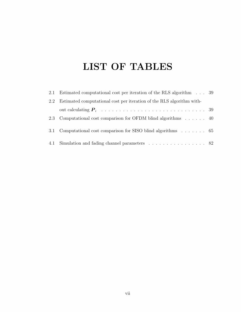
LIST OF TABLES

2.1 Estimated computational cost per iteration of the RLS algorithm . . . 39

2.2 Estimated computational cost per iteration of the RLS algorithm with-

out calculating P i . . . . . . . . . . . . . . . . . . . . . . . . . . . . . 39

2.3 Computational cost comparison for OFDM blind algorithms . . . . . . 40

3.1 Computational cost comparison for SISO blind algorithms . . . . . . . 65

4.1 Simulation and fading channel parameters . . . . . . . . . . . . . . . . 82

vii

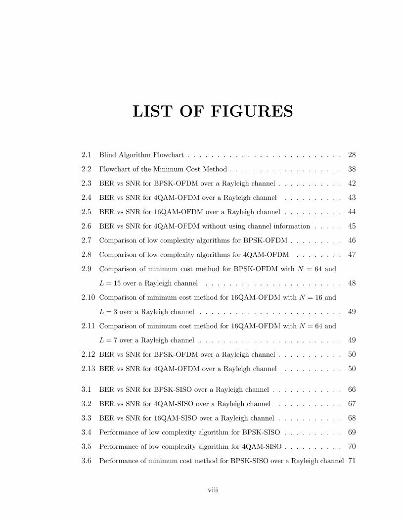
LIST OF FIGURES

2.1 Blind Algorithm Flowchart . . . . . . . . . . . . . . . . . . . . . . . . . . 28

2.2 Flowchart of the Minimum Cost Method . . . . . . . . . . . . . . . . . . . 38

2.3 BER vs SNR for BPSK-OFDM over a Rayleigh channel . . . . . . . . . . . 42

2.4 BER vs SNR for 4QAM-OFDM over a Rayleigh channel . . . . . . . . . . 43

2.5 BER vs SNR for 16QAM-OFDM over a Rayleigh channel . . . . . . . . . . 44

2.6 BER vs SNR for 4QAM-OFDM without using channel information . . . . . 45

2.7 Comparison of low complexity algorithms for BPSK-OFDM . . . . . . . . . 46

2.8 Comparison of low complexity algorithms for 4QAM-OFDM . . . . . . . . 47

2.9 Comparison of minimum cost method for BPSK-OFDM with N = 64 and

L = 15 over a Rayleigh channel . . . . . . . . . . . . . . . . . . . . . . . 48

2.10 Comparison of minimum cost method for 16QAM-OFDM with N = 16 and

L = 3 over a Rayleigh channel . . . . . . . . . . . . . . . . . . . . . . . . 49

2.11 Comparison of minimum cost method for 16QAM-OFDM with N = 64 and

L = 7 over a Rayleigh channel . . . . . . . . . . . . . . . . . . . . . . . . 49

2.12 BER vs SNR for BPSK-OFDM over a Rayleigh channel . . . . . . . . . . . 50

2.13 BER vs SNR for 4QAM-OFDM over a Rayleigh channel . . . . . . . . . . 50

3.1 BER vs SNR for BPSK-SISO over a Rayleigh channel . . . . . . . . . . . . 66

3.2 BER vs SNR for 4QAM-SISO over a Rayleigh channel . . . . . . . . . . . 67

3.3 BER vs SNR for 16QAM-SISO over a Rayleigh channel . . . . . . . . . . . 68

3.4 Performance of low complexity algorithm for BPSK-SISO . . . . . . . . . . 69

3.5 Performance of low complexity algorithm for 4QAM-SISO . . . . . . . . . . 70

3.6 Performance of minimum cost method for BPSK-SISO over a Rayleigh channel 71

viii

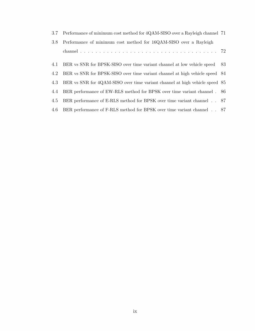
3.7 Performance of minimum cost method for 4QAM-SISO over a Rayleigh channel 71

3.8 Performance of minimum cost method for 16QAM-SISO over a Rayleigh

channel . . . . . . . . . . . . . . . . . . . . . . . . . . . . . . . . . . . . 72

4.1 BER vs SNR for BPSK-SISO over time variant channel at low vehicle speed 83

4.2 BER vs SNR for BPSK-SISO over time variant channel at high vehicle speed 84

4.3 BER vs SNR for 4QAM-SISO over time variant channel at high vehicle speed 85

4.4 BER performance of EW-RLS method for BPSK over time variant channel . 86

4.5 BER performance of E-RLS method for BPSK over time variant channel . . 87

4.6 BER performance of F-RLS method for BPSK over time variant channel . . 87

ix

THESIS ABSTRACT

NAME: Ala′ Ahmad Dahman

TITLE OF STUDY: Low Complexity Blind Equalization for SISO Systems

with General Constellations

MAJOR FIELD: Telecommunication Engineering

DATE OF DEGREE: JUNE 2010

The demand for high data rate reliable communications poses great challenges to the

next generation wireless systems in highly dynamic mobile environments. In this The-

sis, we focus on the blind receiver design for SISO transmission over block fading and

time-variant channels. We investigate the joint Maximum-Likelihood (ML) channel

estimation and data detection for SISO wireless systems with general constellations

and propose a low complexity blind algorithm for finding the exact joint ML solu-

tion. The method uses some a priori information about the communication problem

to improve the channel estimation accuracy and bit error rate. The thesis considers

two SISO systems; circular (OFDM systems) and linear convolution systems. In the

circular convolution system, we show how an OFDM symbol, transmitted over block

fading channel, can be blindly detected using the output symbols only. In the linear

x

convolution system, we perform a blind equalization for a data packet transmitted

over block fading channel using the received symbols only. Finally, the thesis consid-

ers a more realistic problem in which we design a blind receiver for linear convolution

SISO transmission over time-variant channels.

xi

xii

خالصة الرساله

: عالء أحمد دهماناالسم الكامل

: المساواه العمياء قليلة التعقيد ألنظمة القناه احادية المدخل والمخرج عنوان الرساله (SISO) لمجموعات النقاط (Constellations).العامه

: هندسة االتصاالتالتخصص

2010: يونيو تاريخ الشهاده

الطلب على معدالت بث عالية للبيانات بشكل موثوق في أنظمة االتصاالت يفرض تحديات كبيره على الجيل القادم في SISOالنظمةاالنظمه الالسلكيه في بيئات كثيرة الحركه. في هذه الرساله تم التركيز على تصميم جهاز استقبال

(Maximum Likelihood). استخدمنا االحتماليه القصوى block fadingلقنوات متغيرة مع الزمن وقنوات ال النقاط الالسلكيه لمجموعاتSISOالمشتركه لتقدير قنوات البث والكشف عن المعلومات المرسله في أنظمة ال

(Constellations) العامه، واقتراح خوارزميه عمياء قليلة التعقيد اليجاد االحتماليه القصوى المشتركه. هذه الطريقه تستخدم بعض المعلومات المسبقه عن نظام االتصال لتحسين دقة التقدير وخفض معدل االخطاء. الرساله

الدائري (انظمة مضاعفة االنقسام الترددي المتعامد convolution، االول انظمة ال SISOتعتمد اثنين من انظمة ال (OFDM) والثاني انظمة ال ،(convolution الخطي. في النظام االول بيينا كيف ان رمز ال OFDM المرسل عبر يمكن كشفه بشكل أعمى. اما في النظام الثاني فقد أجرينا مساواه عمياء لحزمة بيانات block fadingقنوات ال

باستخدام الرمز المستقبل من القناه فقط. في الجزء االخير من الرساله تم block fadingمرسله عبر قنوات ال الخطي المرسله عبر قنوات convolutionاعتماد نظام أكثر واقعيه حيث تم تصميم جهاز استقبال أعمى ألنظمة ال

متغيره مع الزمن.

CHAPTER 1

INTRODUCTION

In a wireless system, data is sent over a time variant fading channel. At the receiver,

we get the received signal convolved and corrupted with noise. Naturally we are

interested in recovering the transmitted data. Suppose we have information about

the channel over which the data is being transmitted. In this case, we can faithfully

obtain the transmitted data by making use of the received signal and the channel

information (through equalization). In reality, we do not have the prior knowledge of

the transmission channel, and hence we have to settle for an estimate of the channel

obtained at the receiver using some estimation technique. Channel estimation is thus

an important step in receiver design. In a communication system, the sole purpose of

the channel estimation is to recover the transmitted data.

The receiver in the wireless transmission systems must estimate the channel effi-

ciently and subsequently the data in order to achieve high data rate. The receiver

also needs to be of low complexity and should not require too much overhead. The

problem becomes especially challenging in the wireless environment when the channel

1

is time-variant. This Thesis is concerned with blind receivers for linear and circular

convolution SISO systems over block fading and time-variant channels.

This introductory chapter sets the stage for the Thesis. It starts by discussing the

need for channel estimation in Section 1.1. The chapter then presents an overview

of the various channel estimation techniques that have been proposed in literature.

We conclude the chapter by laying out the contributions of the subsequent chapters

in Section 1.3 which also serve to outline the Thesis organization. In Section 1.4, we

introduce our notation.

1.1 The Need for Channel Estimation in a Wireless

Environment

In circular convolution SISO systems, a cyclic prefix (CP) is appended to the trans-

mitted symbol. This allows OFDM to deal effectively with ISI by transforming the

equalization problem into parallel single tap equalizers, while in linear convolution

SISO systems, the equalization design becomes difficult because of the appearance

of the ISI. In both cases, the equalizer taps need to be estimated in the wireless

environment. These taps are usually time variant for a wireless channel. So it be-

comes essential for the receiver to estimate the channel continuously for proper data

detection.

In the following, we summarize the major requirements in receiver design (channel

estimation and data detection). The receiver needs to:

2

1. Deal with time variant channels

The receiver needs to be able to deal with mobility, i.e. with time-variant chan-

nels. In doing so, the receiver needs to take care of the following constraints

Reduce training overhead: The easiest way to deal with time-variant chan-

nels is to send enough pilots. Since, the channel impulse response (IR) can be

as long as the CP of the OFDM symbol, which is roughly one-fourth the OFDM

symbol length [5], each symbol would waste one-fourth of the throughput in

training. Thus, the circular convolution SISO system receiver should employ

more intelligent techniques for channel estimation that would avoid the need for

excessive training and deal with time-variant channels.

Avoid any latency by relying on the current symbol only: Some tech-

niques for channel estimation might deal with the lack of enough training by

relying on past or future symbols to perform some averaging-based channel esti-

mation as is the case with many blind-based estimation techniques. This inher-

ently assumes that the channel remains constant over several data packets which

might not be true in a wireless scenario. Even if the channel is correlated from

one packet to another, a filtering or smoothing approach to channel estimation

requires excessive storage and results in undesirable latency.

Thus, the proper answer to time-variant channels is to use as much natural

structure as possible in the current data packet. This includes 1) The cyclic

prefix in OFDM, 2) the finite alphabet constraint on the data, and 3) the channel

3

finite delay spread and correlation, and rely as little as possible on smoothing

or averaging techniques.

2. Reduce complexity and storage requirements

As pointed out above, the algorithm should bootstrap itself from the current

packet without need for storing past data and especially without having to rely

on the future symbols. The bootstrap should not also come at the expense of

increased complexity.

3. Deal with special channel conditions

The receiver should be able to deal with some special channel conditions which

include

Time variation within the data packet: For applications with high mo-

bility, the receiver should be able to deal with channels that vary within the

data packet which gives rise to interference. However, a prerequisite for solving

this problem is the ability to design a receiver that can cope with the milder

block-fading variation problem 1.

CP length shorter than the length of channel impulse response in

OFDM: This is usually dealt with by using some channel impulse response

shortening techniques.

1This Thesis focuses on the block fading model for OFDM system and both channelmodel (block fading and time-variant channels) for linear SISO system.

4

1.2 Techniques for Channel Estimation and Data

Detection

As mentioned in the introduction, our aim is to design Blind algorithm for channel

estimation and data detection. In this section, we will take a look at the literature

relating to channel estimation and data detection. We will provide an overview of

the various approaches to channel estimation and the different constraints assumed

on channel and data.

The availability of an accurate channel transfer function estimate is one of the

prerequisites for coherent symbol detection in the receiver. Numerous research contri-

butions have appeared in literature on the topic of channel estimation, in recent years.

One way to classify these works is as according to the method used for channel estima-

tion (training based, semi blind, blind and data aided). Another approach to classify

these algorithms is based on the constraints used for channel and data recovery.

1.2.1 Constraints Used in Channel Estimation and Data De-

tection

In literature, all algorithms for channel estimation use some inherent structure of the

communication problem. This structure is produced by constraints on the data or the

channel. In the following, we categorize the research work done on channel estimation

on the basis of the constraints used.

5

Data Constraints

Finite alphabet constraint: Data is usually drawn from a finite alphabet [4], [34],

[35], [57], [58].

Code: Data is coded before being transmitted which introduces redundancy and helps

in reducing probability of error [27], [28], [31], [33], [47]-[50], [56].

Transmit precoding: Precoding might be done on the data at the transmitter to

assist channel estimation at the receiver such as cyclic prefix in OFDM [4], [25],

[30], [31], [40], [46], zero padding (silent guard bands) [8], [9], [10] and virtual

carriers (the subcarriers that are set to zero without any information) [42], [43],

[44], [63].

Pilots: Pilots i.e. training symbols for the receiver, have been extensively used for

channel estimation [11]-[23].

Channel Constraints

Finite delay spread: The length of channel impulse response is considered to be

finite and known to the receiver.

Frequency correlation: It is assumed that some additional statistical information

about the channel taps is known. This is usually captured by the frequency

correlation in the frequency response of the channel taps [4], [12], [31], [51], [59].

Time correlation: As channels vary with time, they show some form of time corre-

lation. In a wireless environment, it is introduced by the doppler effect [4], [10],

6

[33], [52], [54].

1.2.2 Approaches to Channel Estimation and Data Detection

The algorithms used for channel estimation can also be divided on the basis of ap-

proach used. These approaches can be divided into four main categories.

Training based Estimation

Pilots i.e. symbols which are known to the receiver are sent with the data symbols so

that the channel can be estimated and hence the data at the receiver (see [11]-[23]).

Use of training sequences decreases the system bandwidth efficiency [24] and they

are suitable only if the channel is assumed to be time-invariant. But as the wireless

channel is time-varying, it becomes essential to transmit pilots periodically to keep

track of the varying channel. Thus this further decreases the channel throughput.

Blind Estimation

The above limitations in training based estimation techniques motivated interest in the

spectrally efficient blind approach. Only natural constraints are used for estimation

in blind algorithms. For example, cyclic prefix and the cyclostationarity introduced

by it was used by [25], [26], [29], [30], and [46] while coding was also used along with

cyclic prefix by [31]. Redundant and non-redundant linear precoding was exploited in

[27], [28], [33], [47]-[50] for channel estimation. Virtual carriers have also been used

by [42]-[44] and constant modulus modulation was used by [45]. Receiver diversity

was used in [36] while [37]-[41], [44] and the references therein developed a subspace

7

approach using the second order statistics. The finite alphabet constraint on the data

was explored by [34] and [35] and for reducing the computational complexity involved

in it, adaptive techniques were explored by [32] and [33].

Semiblind Estimation

Semiblind techniques make use of both pilots and the natural constraints to efficiently

estimate the channel. These methods use pilots to obtain an initial channel estimate

and improve the estimate by using a variety of a priori information. Thus, in addition

to the pilots, semiblind methods use the cyclic prefix [4], [31], [40], the finite alphabet

constraint on the data as well as the frequency and time correlation of the channel

[4], magnitude error in data [55], linear precoding [56], frequency correlation [12],

[31], and [59], gaussian assumption on transmitted data [60], the first order statistics

[61], subspace of the channel [62], receiver diversity and virtual carriers [63] for channel

estimation and subsequent data detection. Semiblind adaptive approaches for channel

estimation have also been exploited by [57] and [58] who in addition to pilots, utilized

the finite alphabet nature of data and the second order statistics of the received signal,

respectively.

Data-aided Estimation

The purpose of channel estimation is to use that estimate to detect data. The re-

covered data, in turn, can also be used to improve the channel estimate, thus giving

rise to an iterative technique for channel and data recovery. This idea is the basis of

joint channel estimation and data detection. This iterative technique was used in a

8

data-aided fashion by [39] or more rigourously by the expectation maximization (EM)

approach [68]-[73].

1.3 Overview of Contributions

1.3.1 Blind equalization for circular convolution SISO sys-

tems

In Chapter 2, we propose a totally blind algorithm for data detection by using the

output observations only for circular convolution SISO systems (OFDM systems) em-

ploying data with general constellation. Our approach is based on [97] which proposed

the joint Maximum-Likelihood (ML) channel estimation and signal detection problem

for Single-Input Multiple-Output (SIMO) wireless systems. This algorithm rely on

computing the cost function up to the time index i of the data symbols and compare

it with an estimate value (radius) of the optimal solution of the cost function. We

have extended this approach to OFDM system. In that chapter, we propose approxi-

mate methods to reduce the computational complexity involved in the new algorithm.

A new pilot based estimation technique has also been proposed. Specifically, in this

method, data is recovered by finding the constellation point that minimizing the cost

function. As all standard-based OFDM systems involve some form of training, we

have also studied the behavior of the blind receiver in the presence of pilots (training

symbols).

9

1.3.2 Blind equalization for linear convolution SISO systems

In Chapter 3, we consider blind receiver design for linear convolution SISO trans-

mission employing data with general constellation over block fading channels. The

receiver employs the maximum likelihood (ML) algorithm for joint channel and data

recovery, where the blind algorithm used in chapter 2 has been extended to linear con-

volution SISO systems. In that chapter, we also propose an approximate method to

reduce the computational complexity involved in the blind algorithm where the Fast

RLS algorithm has been utilized. A new equalization technique has also been proposed

when the receiver has perfect or estimated knowledge of the channel. Specifically, in

this method, data is recovered by finding the constellation point that minimizing the

cost function.

1.3.3 Blind equalization for linear convolution SISO systems

over time-variant channel

In Chapter 4, we solve a more realistic problem where we design a blind receiver for

channel estimation and data recovery for linear convolution SISO transmission over

time-variant channels. The receiver uses some possible constraints on the channel

(the finite delay spread and frequency and time correlation) and the data (the finite

alphabet constraint). Our approach is based on [97] which proposed the joint ML

channel estimation and signal detection problem for SIMO wireless systems over block

fading channel. We have extended this approach to SISO transmission over time-

variant channel. Three modification/extensions of the RLS algorithm were employed

10

by the new blind algorithm to track the channel and time diversity which include the

exponentially weighted RLS, the Fast RLS and the Extended RLS algorithm. We

have also discussed the effect of the time variation parameters on the performance of

the receiver.

1.4 Notation

We summarize here our notational guidelines for ease of reference. We denote scalars

with small-case letters (e.g. x), vectors with small-case boldface letters (e.g. x), and

matrices with uppercase boldface letters (e.g. X). Calligraphic notation (e.g. X ) is

reserved for vectors in the frequency domain. The individual entries of a vector like h

are denoted by h(l). A hat over a variable indicates an estimate of the variable (e.g.,

h is an estimate of h). When any of these variables become a function of time, the

time index i appears as a subscript. We use the superscript ∗ to denote transposition

with complex conjugation.

11

CHAPTER 2

BLIND EQUALIZATION FOR

CIRCULAR CONVOLUTION

SISO SYSTEMS

2.1 Introduction

The motive of modern broadband wireless communication systems is to offer high

data rate services. The main hindrance for such high data rate systems is multipath

fading as it results in inter-symbol interference (ISI). It therefore becomes essential

to use such modulation techniques that are robust to multipath fading. Multicar-

rier techniques especially Orthogonal Frequency Division Multiplexing (OFDM) has

emerged as a modulation scheme that can achieve high data rate by efficiently han-

dling multipath effects. The additional advantages of simple implementation and high

spectral efficiency due to orthogonality contribute towards the increasing interest in

12

OFDM. This is reflected by the many standards that considered and adopted OFDM,

including those for digital audio and video broadcasting (DAB and DVB), WIMAX

(Worldwide Interoperability for Microwave Access), high speed modems over digital

subscriber lines, and local area wireless broadband standards such as the HIPER-

LAN/2 and IEEE 802.11a, with data rates of up to 54 Mbps [1]. OFDM is also being

considered for fourth-generation (4G) mobile wireless systems [2].

In order to achieve high data rate in OFDM, the receivers must be well designed

i.e. it must estimate the channel efficiently and subsequently the data. The receiver

also needs to be of low complexity and should not require too much overhead. The

problem becomes especially challenging in the wireless environment when the channel

is time-variant. Several blind channel estimation algorithms have been devised for

OFDM systems. Some of them are based on a subspace approach exploiting the

cyclostationary property that is inherent to OFDM transmissions in the cyclic prefix

[100] [26]. Another type of blind channel estimator capitalizes on the finite alphabet

property of the modulated symbols [39]. Many other techniques have been proposed

in the literature for this purpose too (see, e.g., [1], [4], [99], [98]).

In this chapter, we propose a low complexity algorithm for blind equalization

in circular convolution SISO systems (OFDM systems) employing data with general

constellations. The algorithm is able to recover the data from the output observations

only. This is done for one OFDM symbol allowing the algorithm to work in block

fading channels.

13

2.1.1 The Approach and Organization of the Chapter

This chapter proposes a blind receiver for the OFDM systems by using a new al-

gorithm, which showed a favorable performance whether operating in the blind or

training modes.

In the first part of the chapter, we perform data estimation and equalization from

output observations only, without the need for a training sequence or a priori channel

information. The advantage of our approach is three fold:

1. The method provides a blind estimate of the data from one output symbol

without the need for training. Thus, the method lends itself to block fading

channels.

2. The algorithm works on OFDM systems employing data with general constella-

tions.

3. Data equalization is done without any restriction on the channel

We start with setup the OFDM system model in Section 2.2. Our approach is based

on joint maximum-likelihood (ML) channel estimation and signal detection problem

for OFDM wireless systems with general modulation constellations and propose an

efficient algorithm for finding the exact joint ML solution (see Section 2.3). The

algorithm takes a particularly simple form in constant modulus case (see Section 2.4).

The new blind algorithm can be computationally expensive with two drawbacks

explained in Section 2.5. We thus suggest in the second part of the chapter (Sections

2.6 and 2.7), three approaches to reduce this computational complexity. In the first

14

and second approaches, we try to simplify the new algorithm by avoiding the need

of calculating one of its big matrices. In the third approach, we propose a very

low complexity method to detect the data based on the minimum cost. These three

methods have different complexity, thus we compare their computational complexity

in Section 2.8. Simulation results are discussed in Section 2.9 with conclusion in

Section 2.10.

2.2 System Overview

2.2.1 Notation

Consider a length-N vector xi. We deal with three derivatives associated with this

vector. The first two are obtained by partitioning xi into a lower (trailing) part xi

(known as the cyclic prefix) and an upper vector xi so that

xi =

xi

xi

The third derivative, xi, is created by concatenating xi with a copy of CP i.e. xi.

Thus, we have

xi =

xi

xi

=

xi

xi

xi

(2.1)

15

In line with the above notation, a matrix Q having N rows will have the natural

partitioning

Q =

Q

Q

(2.2)

where the number of rows in Q and Q are understood from the context and when it

is not clear, the number of rows will appear as a subscript.Thus, we write

Q =

QN−L

QL

(2.3)

2.2.2 System Model

In an OFDM system, data is transmitted in symbols X i of length N each. The symbol

undergoes an IFFT operation to produce the time domain symbol xi, i.e.

xi =√

NQX i (2.4)

where Q is the N × N IFFT matrix. When juxtaposed, these symbols result in

the sequence xk. 1 We assume a channel h of maximum length L + 1. To avoid

ISI caused by passing through the channel, a cyclic prefix (CP) xi (of length L) is

appended to xi, resulting in super-symbol xi as defined in (2.1). The concatenation

of these symbols produces the underlying sequence xk. When passed through the

1The time indices in the sequence xi and the underlying sequence xk are dummy vari-ables. Nevertheless, we chose to index the two sequences differently to avoid any confusionthat might arise from choosing identical indices.

16

channel h, the sequence xk produces the output sequence yk i.e.

yk = hk ∗ xk + nk (2.5)

where nk is the additive white Gaussian noise and ∗ stands for linear convolution.

Motivated by the symbol structure of the input, it is convenient to partition the

output into length N + L symbol as

yi =

yi

yi

This is a natural way to partition the output because the prefix yiactually absorbs

all ISI that takes place between the adjacent symbols xi−1 and xi. Moreover, the

remaining part yi of the symbol depends on the ith input OFDM symbol xi only.

These facts can be seen from the input/output relationship

yi−1

yi

yi

=

H

OL×N HU

ON×N ON×L

ON×L ON×N

HL OL×N

H

xi−1

xi−1

xi−1

xi

xi

xi

+

ni−1

ni

ni

(2.6)

where n is the output noise which we take to be white Gaussian. The matrices H ,

HL, and HU are convolution (Toeplitz) matrices of proper sizes created from the

17

vector h. Specifically, H is the N × (N + L) matrix

H =

h(L) · · · h(1) h(0)

.... . . · · · . . . . . .

0 · · · h(L) · · · h(1) h(0)

(2.7)

The matrices HU and HL are square of size L.2

HU =

h(L) h(L− 1) · · · h(1)

h(L) · · · h(2)

. . ....

h(L)

(2.8)

HL =

h(0)

h(1) h(0)

.... . . . . .

h(L− 1) · · · h(1) h(0)

(2.9)

2The matrix HL (HU) is lower (upper) triangular; this explains the superscript L (U).

18

2.2.3 Circular Convolution

From (2.6), we can write

yi = H

xi

xi

xi

= H xi + ni (2.10)

This shows that yi is created solely from xi through convolution and hence is ISI-free.

Moreover, the existence of a cyclic prefix in xi allows us to rewrite (2.10) as

yi = Hxi + ni (2.11)

where H is the size-N circulant matrix.

H =

h(0) 0 · · · 0 h(L) · · · h(1)

h(1) h(0) · · · 0 0 · · · h(2)

......

. . .... · · · . . .

...

h(L) h(L− 1) · · · h(0) 0 · · · 0

.... . . . . . · · · . . .

......

0 0 · · · h(L) h(L− 1) · · · h(0)

(2.12)

In other words, the cyclic prefix of xi renders the convolution in (2.11) cyclic, and we

can write

yi = hi∗xi + ni (2.13)

19

where ∗ is the circular convolution, and hi is a length-N zero-padded version of hi.

hi =

hi

O(N−L−1)×1

In the frequency domain, the circular convolution (2.13) reduces to the element-by-

element operation

Y i = Hi ¯X i + N i (2.14)

where ¯ stands for element-by-element multiplication and where Hi, X i, N i, and Y i,

are the DFT’s of hi, xi, ni, and yi respectively

Hi = Q∗hi, X i =1√N

Q∗xi, N i =1√N

Q∗ni, and Y i =1√N

Q∗yi (2.15)

Since hi corresponds to the first L + 1 elements of hi, we can show that

Hi = A∗hi and hi = AHi (2.16)

where A∗ consists of the first L + 1 columns of Q∗ and A consists of first L + 1 rows

of Q . This allows us to rewrite (2.14) as

Y i = diag(X i)A∗hi + N i (2.17)

20

2.3 Blind Equalization Approach

Consider input/outout equation (2.14), reproduced here for convenience

Y = H¯X + N (2.18)

= diag(X )H + N (2.19)

Element by element, this equation can be written as

Y(j) = X (j)H(j) +N (j)

or since H = A∗h,

Y(j) = X (j)a∗jh +N (j)

where a∗j is the jth row of A∗ (so that aj is the jth column of A).

The problem of joint ML channel estimation and data detection for OFDM chan-

nels is transformed into the following minimization problem

J = minh,X∈ΩN

‖Y − diag(X )A∗h‖2 (2.20)

= minh,X∈ΩN

N∑i=1

|Y(i)−X (i)a∗i h|2 (2.21)

= minh,X∈ΩN

i∑j=1

|Y(j)−X (j)a∗jh|2 +N∑

j=i+1

|Y(j)−X (j)a∗jh|2 (2.22)

where ΩN denotes the set of N−dimensional signal vector.

21

Let us consider a partial data sequence X (i) up to the time index i i.e.

X (i) = [X (1) X (2) · · · X (i)]

and define MX(i)as the cost function of the first i data symbols, say

MX(i)= ‖Y (i) − diag(X (i))A

∗(i)h‖2 (2.23)

where A∗(i) consists of the first i rows of A∗.

Now, as per Weiyu’s paper [97], let R be the optimal value for our objective

function in (2.20), if MX(i)> R, then X (i) can not be the first i symbols of the ML

solution X (i) to (2.20). To prove this, suppose X (i) = X (i) and we denote the optimal

channel gains corresponding to X (i) as h. Then

R = ‖Y (i) − diag(X (i))A∗(i)h‖2 +

N∑j=i+1

|Y(j)− X (j)a∗j h|2 (2.24)

≥ minh‖Y (i) − diag(X (i))A

∗(i)h‖2 +

N∑j=i+1

|Y(j)− X (j)a∗j h|2 (2.25)

≥ minh‖Y (i) − diag(X (i))A

∗(i)h‖2 = MX(i)

= MX(i)(2.26)

So, for X (i) to correspond to the first i symbols of the ML solution X (i), we should have

MX(i)< R. Note that the above represents a necessary condition only in that if X (i)

is such that MX(i)< R, then that does not necessarily mean that X (i) coincides with

X (i). In the next subsection (2.3.1), we will use this properly in our blind algorithm.

Since A∗(i) is full rank for i ≤ L + 1, diag(X (i))A

∗(i) is full rank too for each choice

22

of diag(X (i)) and so we will always find some h that will make the first part of the

objective function zero (since h has exactly L + 1 degrees of freedom). Thus, our

search tree should be at least of depth L + 1. This explains why L + 1 pilots are

needed in OFDM. To reduce the search space, we could use p pilots (p < L + 1) and

hence need only deal with a tree of depth L+1− p (without loss of generality, we can

place all pilots at the beginning of the symbol X ).

Assuming that we have some initial guess, let’s see how we can update the objective

function when we move down the tree by one level. The objective function can be

updated according to some recursion. Specifically, assume that we obtained the cost

function involved in minimizing

MX(i−1)= ‖Y (i) − diag(X (i))A

∗(i)h‖2

and we would like to obtain the cost function for the next iteration. From the above

discussion, we know that MX(i)= 0 for i ≤ L + 1. For i > L + 1, the cost can be

obtained using Recursive Least Squares (RLS) algorithm [92] by the following set of

iterations

MX(i)= MX(i−1)

+ γ(i)|Y(i)−X (i)a∗i hi−1|2 (2.27)

hi = hi−1 + gi(Y(i)−X (i)a∗i hi−1) (2.28)

23

where

gi = γ(i)X ∗(i)P i−1ai (2.29)

γ(i) =1

1 + |X (i)|2a∗i P i−1ai

(2.30)

P i = P i−1 − γ(i)|X (i)|2P i−1aia∗i P i−1 (2.31)

The recursions are initialized by

MX(L+1)= 0, P L+1 =

(A(L+1)diag(|X (i)|2)Q∗

(L+1)

)−1,

and hL+1 = P L+1A(L+1)diag(X ∗(i))Y (i)

Now since h has L + 1 degrees of freedom, we need L + 1 pilots to identify it, or

alternatively, we need to guess L + 1 solutions before we can move on. The reason is

that h has L + 1 degrees of freedom.

We could also calculate the cost function without obtaining the actual value of the

solution hi using the recursion

MX(i)= Y∗

(i)

(I − diag(X (i))A

∗(i)P iA(i)diag(X ∗

(i)))−1 Y (i) (2.32)

with P i calculated recursively as in above. However, this solution is computationally

more complex than the RLS solution above.

The problem with the above approach is that we need to have the value of L + 1

X (i)′s before starting to have a nonzero value for the objective function. An alterna-

24

tive strategy would be to find h using weighted regularized least squares. Specifically,

instead of minimizing the objective function J in equation (2.20), we minimize

J = minh,X∈ΩN

‖h‖2R−1

h+ ‖Y − diag(X )A∗h‖2

R−1n

(2.33)

= minh,X∈ΩN

‖h‖2R−1

h+

1

σ2

N∑i=1

|Y(i)−X (i)a∗i h|2 (2.34)

where Rh is some weighting matrix that could be taken as the autocorrelation matrix

of h and Rn is the autocorrelation matrix of the noise given by σ2I, where σ2 is the

noise variance. With this modification, we can recursively calculate the value of the

objective function for each i through the following set of recursions similar to the ones

we have above, and we called it through this chapter as Blind RLS Algorithm:

MX(i)= MX(i−1)

+ 1σ2 γ(i)|Y(i)−X (i)a∗i hi−1|2 (2.35)

hi = hi−1 + 1σgi

(Y(i)−X (i)a∗i hi−1

)(2.36)

where

gi =1

σγ(i)X (i)∗P i−1ai (2.37)

γ(i) =1

1 + 1σ2 |X (i)|2a∗i P i−1ai

(2.38)

P i = P i−1 − 1

σ2γ(i)|X (i)|2P i−1aia

∗i P i−1 (2.39)

25

except that these recursions apply for all i and are initialized by

MX(−1)= 0, P−1 = Rh, and h−1 = 0

Now, R is the optimal value for the regularized objective function in (2.33), and

MX(i)is the value of the cost function for the sequence X (i) up to the time index i. If

the value R can be estimated, we can restrict the search of the blind ML solution X

to the offsprings of those partial sequences X (i) which satisfy MX(i)< R.

There are three advantages for this second approach:

1. We don’t need to wait for L+1 X (i)’s before starting to get a nonzero objective

function.

2. We don’t need to perform a size L + 1 matrix inversion as in (2.32); instead a

simpler RLS can be performed from the first step.

3. We make use of the channel autocorrelation which will improve the accuracy of

the algorithm.

2.3.1 Exact Blind Algorithm

In this section, we describe the algorithm that we use to find the ML solution of

the system output observations, the algorithm employs the above set of iterations

(2.35)−(2.39) to update the value of the cost function (MX(i)) which we need for the

comparison with the estimated value R (we denote it in the blind algorithm below as

26

the search radius r).

The input parameters for this algorithm are:

• The received channel output Y .

• The search radius r.

• The modulation constellation Ω.

• 1×N index vector I.

We denote the kth constellation point in the modulation constellation Ω as Ω(k).

The following steps explain the process of our algorithm, which we illustrate them

also in the next flowchart (Figure (2.1)):

1. Set i = 1, ri = r, I(i) = 1 and set X (i) = Ω(I(i)).

2. (Computing the bounds) Compute the metric MX(i). If MX(i)

> r, go to 3; else,

go to 4;

3. (Backtracking) Find the largest 1 ≤j ≤i such that I(j) < |Ω|. If there exists

such j, set i = j and go to 5; else go to 6.

4. If i = N, store current X (N), update r = MX(N)and go to 3; else set i =

i + 1, I(i) = 1 and X (i) = Ω(I(i)), go to 2.

5. Set I(i) = I(i) + 1 and X (i) = Ω(I(i)). Go to 2.

6. If any sequence X (N) is ever found in Step 4, output the latest stored full-length

sequence as ML solution; otherwise, double r and go to 1.

27

Figure 2.1: Blind Algorithm Flowchart

2.3.2 Choice of the Initial Radius r

The structure of the new blind ML algorithm easily suggests a probabilistic choice of

the search radius. We know that ‖n‖2 is chisquare distributed with 2N degrees of

freedom, it is natural to choose the radius r such that P (‖n‖2 > r2) ≤ 1− ε. Since

the solution R to the optimization problem in (2.33) is sure to be smaller than ‖n‖2,

we will guarantee finding the blind ML data sequence with probability at least 1 − ε

under this initial radius.

28

2.4 Blind Equalization in the Constant Modulus

Case

As we saw, the backtracking algorithm depends heavily on calculating the cost func-

tion. This operation can be made easier in the constant modulus case.

In this case, the values of 1σ2 |X (i)|2 in equations (2.38) and (2.39) become constant

for all i, so assume that they are equal to 1σ2EX , then the values of γ(i) and P i in the

same equations will become

γ(i) =1

1 + 1σ2EXa∗i P i−1ai

(2.40)

P i = P i−1 − 1

σ2EXγ(i)P i−1aia

∗i P i−1 (2.41)

which are independent of the transmitted signal, and depends only on i, so they are

constant for each OFDM symbol and we can calculate them offline. This case will

reduce the computational complexity as the (L + 1) × (L + 1) matrix P i will be

computed offline and there is no need to update it.

2.5 Drawbacks of the Backtracking Algorithm

Using the above blind algorithm to search for the optimal X can be computationally

very complex due to two main reason:

1. Calculating P i: the second step of the blind algorithm rely on updating the

metric MX(N), This metric depends heavily on calculating the L + 1 × L + 1

29

matrix P i which adds much complexity to the algorithm.

2. Backtracking: the main disadvantage of our blind algorithm include in the

third step where the algorithm try to improve the detection by searching for

best combination of the constellation points that investigate the condition of

MX(i)> r.

In the next two sections, we propose approximate methods to avoid these draw-

backs, where the both drawbacks can be done jointly or independently.

2.6 Approximate Methods to Reduce the Compu-

tational Complexity Involved in Calculating P i

The first drawback makes the blind algorithm more complex due to calculating the

matrix P i at each updating of the metric MX(i). In the following, we describe two

methods to avoid computing this matrix:

2.6.1 Avoiding P i

If we set Rh (the initial value of P i in the RLS algorithm) equal to the Identity Matrix

(I), let’s see how P i looks like, note that in equations (2.37)−(2.39) P i always appears

multiple by ai, so let’s demonstrate how setting P−1 = I will reduce our calculations.

Start with i = 0

γ(0) =1

1 + 1σ2 |X (0)|2a∗0P−1a0

30

where a∗i ai = L + 1 and P−1 = I, then

γ(0) =1

1 + 1σ2 |X (0)|2(L + 1)

and

P 0 = P−1 − 1

σ2γ(0)|X (0)|2P−1a0a

∗0P−1

multiply P 0 by a1

P 0a1 = P−1a1 − 1

σ2γ(0)|X (0)|2a0a

∗0a1

Since ai is truncated length−(L + 1) FFT vector, we can assume that the value of

a∗i ai−1 ≈ a∗i−1ai ≈ 0,3 thus

P 0a1 = Ia1 − 0 = a1 (2.42)

Also, multiply P 0 by a2 to get

P 0a2 = P−1a2 − 1

σ2γ(0)|X (0)|2a0a

∗0a2 (2.43)

= Ia2 − 0 = a2 (2.44)

For i = 1

γ(1) =1

1 + 1σ2 |X (1)|2a∗1P 0a1

3This becomes especially true for large L

31

from the above equation (2.42), P 0a1 = a1, thus

γ(1) =1

1 + 1σ2 |X (1)|2(L + 1)

Since P 0a1 = a1 and P 0a2 = a2 (from equations (2.42) and (2.44), respectively), the

value of P 1a2 is given by

P 1a2 = P 0a2 − 1

σ2γ(1)|X (1)|2P 0a1a

∗1P 0a2 (2.45)

= a2 − 1

σ2γ(1)|X (1)|2a1a

∗1a2 (2.46)

= a2 (2.47)

Now, from the above equations (2.42)-(2.47) we can assume that P iai+1 = ai+1, and

P iai+2 = ai+2, so let’s prove also that P i+1ai+2 = ai+2

P i+1ai+2 = P iai+2 − 1

σ2γ(i + 1)|X (i + 1)|2P iai+1a

∗i+1P iai+2 (2.48)

= ai+2 − 1

σ2γ(i + 1)|X (i + 1)|2ai+1a

∗i+1ai+2 (2.49)

= ai+2 (2.50)

As a result, the values of γ(i) and P iai+1 are given by

γ(i) =1

1 + 1σ2 |X (i)|2(L + 1)

, for i = 0, 1, . . . , N − 1 (2.51)

P iai+1 = ai+1 (2.52)

32

Use this result in our blind RLS algorithm in (2.35)-(2.39) and replace gi and hi

by the following equations.

gi =1

σγ(i)X ∗(i)ai (2.53)

hi = hi−1 + 1σ2 γ(i)[X ∗(i)Y(i)ai − |X (i)|2aia

∗i hi−1] (2.54)

Observe that our blind algorithm remain same except that we don’t need to cal-

culate the value of P i in equation (2.39), which drastically reduces the computational

complexity. In the next section, we shall compare the computational complexity for

this method and the blind RLS algorithm.

Constant Modulus Case

Let’s apply this method to the constant modulus case and see how the calculations

become simpler. We know that the values of 1σ2 |X (i)|2 become constant for all i and

equal to 1σ2EX in the constant modulus case. So the above values of γ(i) and hi in

(2.51) and (2.54), respectively, become

γ(i) =1

1 + 1σ2EX (L + 1)

(2.55)

hi = hi−1 +1

1 + 1σ2EX (L + 1)

(1

σX ∗(i))(

1

σY(i))ai − 1

σ2EXaia

∗i hi−1

take 1σ2 as a common factor

hi = hi−1 + 1σ2+EX (L+1)

X ∗(i)Y(i)ai − EXaia∗i hi−1 (2.56)

33

In addition to the above result of avoiding P i, we also don’t need to calculate γ(i),

this leads to more reduction in the complexity.

2.6.2 Avoiding P i with Ordering A∗i

In the previous subsection we have presented a method to reduce the computational

complexity assuming that Rh = I and a∗i ai−1 ≈ a∗i−1ai ≈ 0. In this subsection, we

suggest a method to make a∗i ai−1 and a∗i−1ai equal to zero, which will improve our

previous method.

We know that a∗i is a truncated length−(L + 1) FFT vector, and multiplying a∗i

by ai−1 is not exactly equal to zero. However, we can order these vectors to become

a full FFT vectors such that the values of a∗i ai−1 and a∗i−1ai become zero. Here, a∗i

is the i−th row of the truncated (N × (L + 1)) FFT matrix A∗

A∗ =

e−j 2πN

(0)(0) e−j 2πN

(0)(1) · · · e−j 2πN

(0)(L)

e−j 2πN

(1)(0) e−j 2πN

(1)(1) · · · e−j 2πN

(1)(L)

......

......

e−j 2πN

(N−1)(0) e−j 2πN

(N−1)(1) · · · e−j 2πN

(N−1)(L)

N×(L+1)

=

a∗0

a∗1

...

a∗N−1

where

a∗n =

[e−j 2π

N(n)(0) e−j 2π

N(n)(1) · · · e−j 2π

N(n)(L)

]for n = 0, 1, ..., N − 1

In OFDM systems, the cyclic prefix is usually chosen to be N4, N

8, N

16, etc. So, let’s

assume that the channel length is equal to the cyclic prefix and take the case of

34

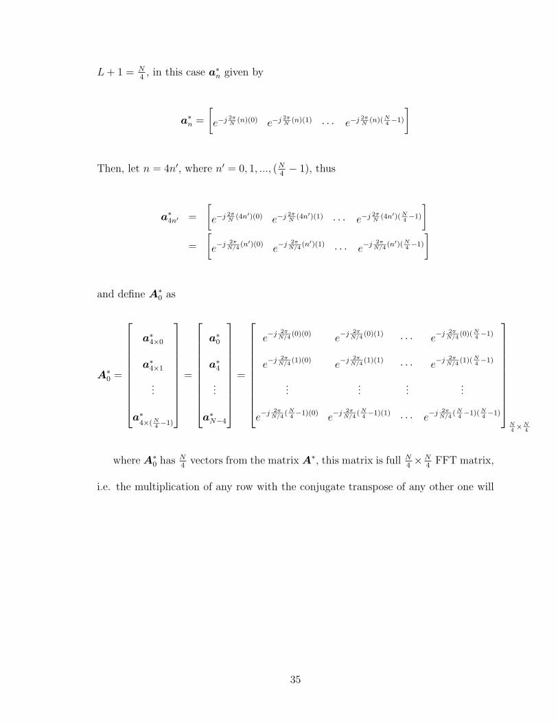
L + 1 = N4, in this case a∗n given by

a∗n =

[e−j 2π

N(n)(0) e−j 2π

N(n)(1) · · · e−j 2π

N(n)(N

4−1)

]

Then, let n = 4n′, where n′ = 0, 1, ..., (N4− 1), thus

a∗4n′ =

[e−j 2π

N(4n′)(0) e−j 2π

N(4n′)(1) · · · e−j 2π

N(4n′)(N

4−1)

]

=

[e−j 2π

N/4(n′)(0) e−j 2π

N/4(n′)(1) · · · e−j 2π

N/4(n′)(N

4−1)

]

and define A∗0 as

A∗0 =

a∗4×0

a∗4×1

...

a∗4×(N

4−1)

=

a∗0

a∗4

...

a∗N−4

=

e−j 2πN/4

(0)(0) e−j 2πN/4

(0)(1) · · · e−j 2πN/4

(0)(N4−1)

e−j 2πN/4

(1)(0) e−j 2πN/4

(1)(1) · · · e−j 2πN/4

(1)(N4−1)

......

......

e−j 2πN/4

(N4−1)(0) e−j 2π

N/4(N

4−1)(1) · · · e−j 2π

N/4(N

4−1)(N

4−1)

N4×N

4

where A∗0 has N

4vectors from the matrix A∗, this matrix is full N

4× N

4FFT matrix,

i.e. the multiplication of any row with the conjugate transpose of any other one will

35

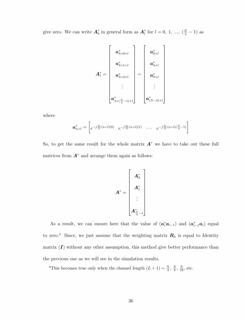
give zero. We can write A∗0 in general form as A∗

l for l = 0, 1, ..., (N4− 1) as

A∗l =

a∗4×0+l

a∗4×1+l

a∗4×2+l

...

a∗4×(N

4−1)+l

=

a∗0+l

a∗4+l

a∗8+l

...

a∗(N−4)+l

where

a∗n+l =

[e−j 2π

N(n+l)(0) e−j 2π

N(n+l)(1) · · · e−j 2π

N(n+l)(N

4−1)

]

So, to get the same result for the whole matrix A∗ we have to take out these full

matrices from A∗ and arrange them again as follows:

A∗ =

A∗0

A∗1

...

A∗N4−1

As a result, we can ensure here that the value of (a∗i ai−1) and (a∗i−1ai) equal

to zero.4 Since, we just assume that the weighting matrix Rh is equal to Identity

matrix (I) without any other assumption, this method give better performance than

the previous one as we will see in the simulation results.

4This becomes true only when the channel length (L + 1) = N4 , N

8 , N16 , etc.

36

2.7 Minimum Cost Method

In addition to calculating the (L+1)×(L+1) matrix P i in the backtracking algorithm,

there is a backtracking operation steps which increase its complexity. In the following,

we describe a method to avoid these steps.

Our objective in data detection is to minimize the cost function. In this method,

we depend on finding the constellation points that minimize the cost function at each

carrier (according to the following equation (2.57)) and take them as a solution without

backtracking.

From (2.35), and for the j-th constellation point (Ω(j)), we can define M jX(i)

as the

cost function up to the time index i, say

M jX(i)

= MX(i−1)+ 1

σ2 γ(i)|Y(i)− Ω(j)a∗i hi−1|2 (2.57)

After we compute all the j values of the cost function, we find the minimum one and

its index (l), then store the l-th constellation point in the i-th solution X (i). The

same procedure is followed for the next carrier up to the one at time N . The following

flowchart (Figure (2.2))explains the processes of our approach. We denote the number

of the constellation points as m.

In this method, there is no need to do backtracking, which gives us a very low

complexity compared with backtracking method (Figure (2.1)) with some sacrifice in

the BER performance as we will show in the simulation results.

In addition, this method can be used as a pilot based channel estimation method

37

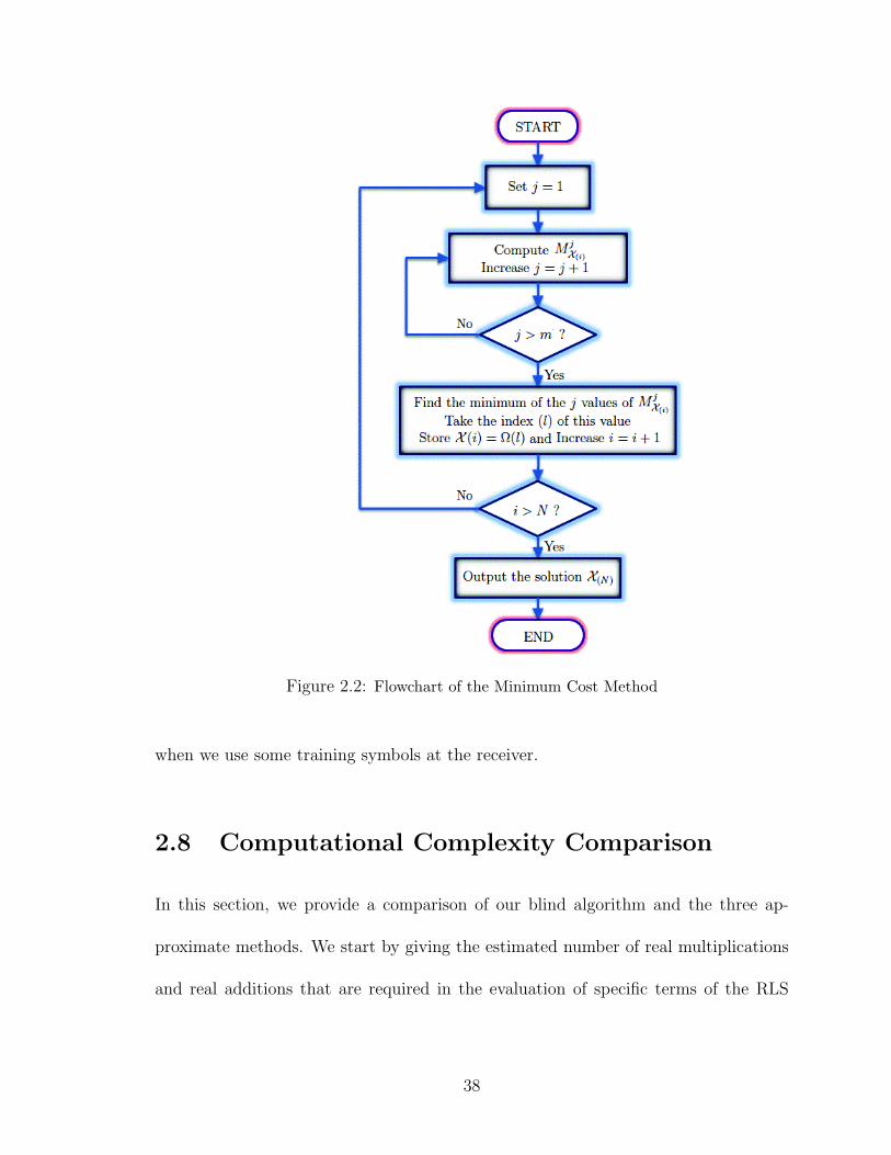
Figure 2.2: Flowchart of the Minimum Cost Method

when we use some training symbols at the receiver.

2.8 Computational Complexity Comparison

In this section, we provide a comparison of our blind algorithm and the three ap-

proximate methods. We start by giving the estimated number of real multiplications

and real additions that are required in the evaluation of specific terms of the RLS

38

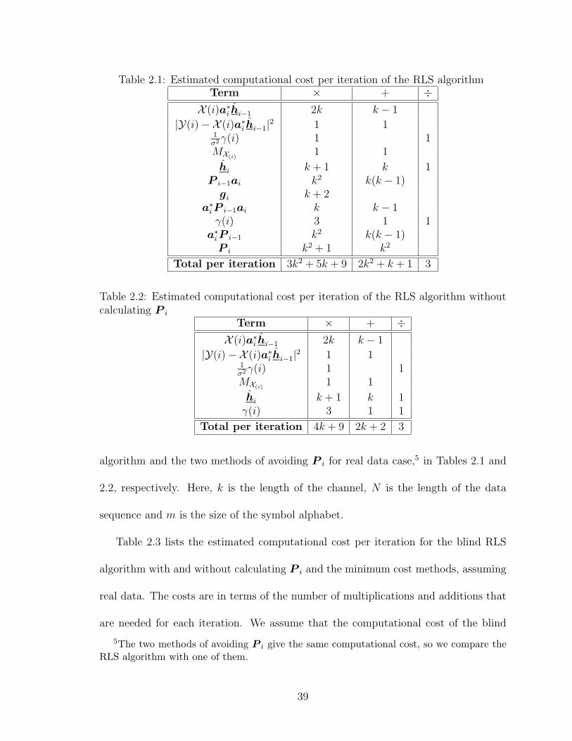
Table 2.1: Estimated computational cost per iteration of the RLS algorithmTerm × + ÷

X (i)a∗i hi−1 2k k − 1

|Y(i)−X (i)a∗i hi−1|2 1 11σ2 γ(i) 1 1MX(i)

1 1

hi k + 1 k 1P i−1ai k2 k(k − 1)

gi k + 2a∗i P i−1ai k k − 1

γ(i) 3 1 1a∗i P i−1 k2 k(k − 1)

P i k2 + 1 k2

Total per iteration 3k2 + 5k + 9 2k2 + k + 1 3

Table 2.2: Estimated computational cost per iteration of the RLS algorithm withoutcalculating P i

Term × + ÷X (i)a∗i hi−1 2k k − 1

|Y(i)−X (i)a∗i hi−1|2 1 11σ2 γ(i) 1 1MX(i)

1 1

hi k + 1 k 1γ(i) 3 1 1

Total per iteration 4k + 9 2k + 2 3

algorithm and the two methods of avoiding P i for real data case,5 in Tables 2.1 and

2.2, respectively. Here, k is the length of the channel, N is the length of the data

sequence and m is the size of the symbol alphabet.

Table 2.3 lists the estimated computational cost per iteration for the blind RLS

algorithm with and without calculating P i and the minimum cost methods, assuming

real data. The costs are in terms of the number of multiplications and additions that

are needed for each iteration. We assume that the computational cost of the blind

5The two methods of avoiding P i give the same computational cost, so we compare theRLS algorithm with one of them.

39

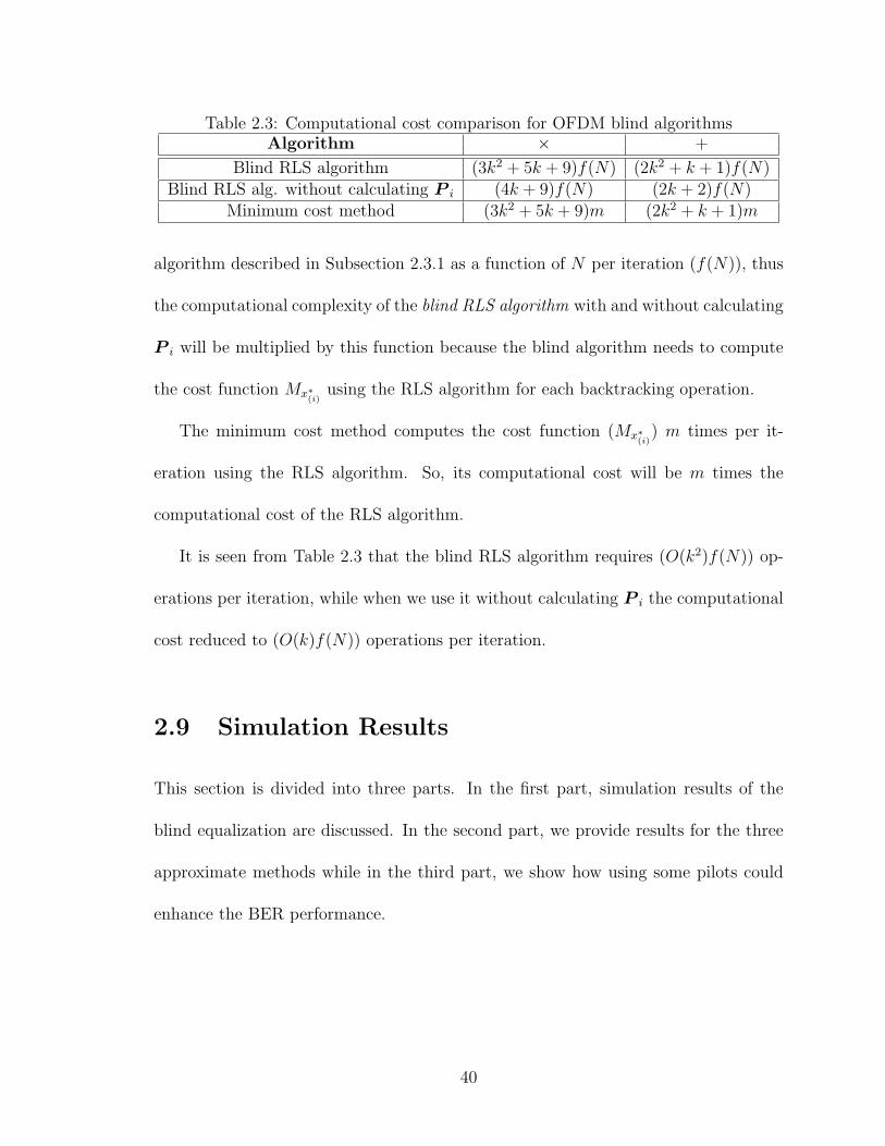
Table 2.3: Computational cost comparison for OFDM blind algorithmsAlgorithm × +

Blind RLS algorithm (3k2 + 5k + 9)f(N) (2k2 + k + 1)f(N)Blind RLS alg. without calculating P i (4k + 9)f(N) (2k + 2)f(N)

Minimum cost method (3k2 + 5k + 9)m (2k2 + k + 1)m

algorithm described in Subsection 2.3.1 as a function of N per iteration (f(N)), thus

the computational complexity of the blind RLS algorithm with and without calculating

P i will be multiplied by this function because the blind algorithm needs to compute

the cost function Mx∗(i)

using the RLS algorithm for each backtracking operation.

The minimum cost method computes the cost function (Mx∗(i)

) m times per it-

eration using the RLS algorithm. So, its computational cost will be m times the

computational cost of the RLS algorithm.

It is seen from Table 2.3 that the blind RLS algorithm requires (O(k2)f(N)) op-

erations per iteration, while when we use it without calculating P i the computational

cost reduced to (O(k)f(N)) operations per iteration.

2.9 Simulation Results

This section is divided into three parts. In the first part, simulation results of the

blind equalization are discussed. In the second part, we provide results for the three

approximate methods while in the third part, we show how using some pilots could

enhance the BER performance.

40

2.9.1 Blind Equalization

In this section, we give simulation results for the performance of the new blind al-

gorithm. We investigate its performance in OFDM system employing BPSK, 4QAM

and 16QAM modulation data where we assume N = 16 carriers and cyclic prefix of

length L = N4− 1. In the simulation, the channel IR consists of L + 1 iid Rayleigh

fading taps which remains constant over one OFDM symbol. We compare the BER

performance of four methods: (i) Perfectly known channel, (ii) Channel estimated

using L + 1 pilots and (iii) The new Blind Algorithm.

BER vs SNR Comparison for BPSK Modulated Data

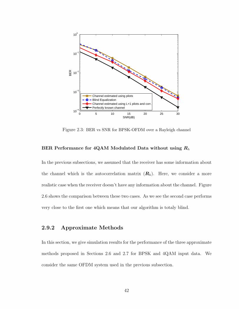
In Figure 2.3, we compare the three mentioned approaches and a semiblind least

squares estimator using L + 1 pilots and frequency correlation, for BPSK modulated

data over a Rayleigh fading channel. As expected, the best performance is achieved

by the perfectly known channel, followed by that obtained by the semiblind least

squares estimator using L + 1 pilots and frequency correlation. The simulation also

shows favorable BER performance of the blind equalization method comparing with

the method that using L + 1 pilots in channel estimation.

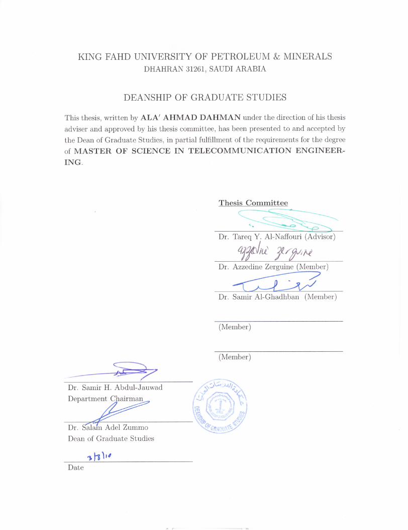
BER vs SNR Comparison for QAM Modulated Data

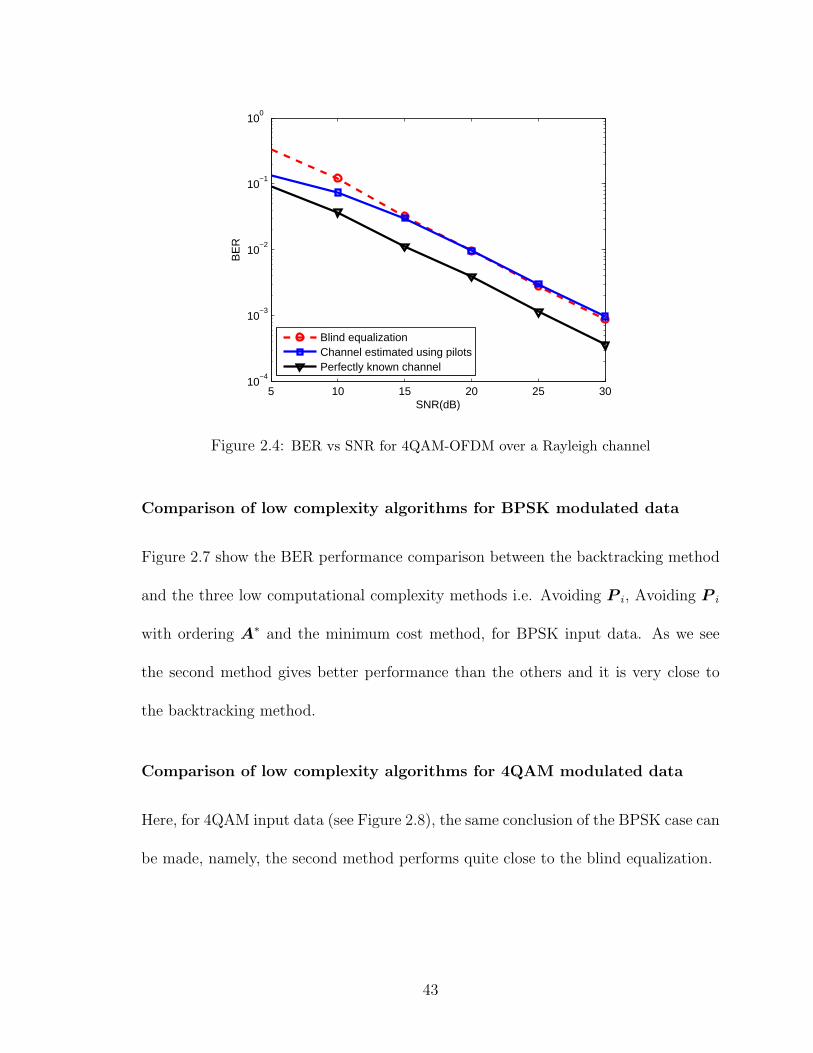
The same conclusion can be made for 4QAM and 16QAM (non-constant modulus)

modulation (see Figures 2.4 and 2.5), where the blind algorithm outperforms the pilot

based estimation method at high SNR.

41

0 5 10 15 20 25 3010

−4

10−3

10−2

10−1

100

SNR(dB)

BE

R

Channel estimated using pilotsBlind EqualizationChannel estimated using L+1 pilots and corr.Perfectly known channel

Figure 2.3: BER vs SNR for BPSK-OFDM over a Rayleigh channel

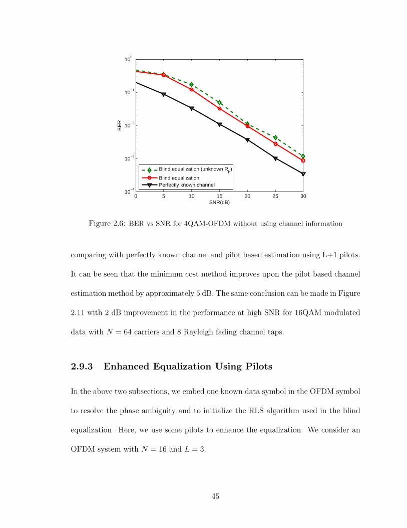
BER Performance for 4QAM Modulated Data without using Rh

In the previous subsections, we assumed that the receiver has some information about

the channel which is the autocorrelation matrix (Rh). Here, we consider a more

realistic case when the receiver doesn’t have any information about the channel. Figure

2.6 shows the comparison between these two cases. As we see the second case performs

very close to the first one which means that our algorithm is totaly blind.

2.9.2 Approximate Methods

In this section, we give simulation results for the performance of the three approximate

methods proposed in Sections 2.6 and 2.7 for BPSK and 4QAM input data. We

consider the same OFDM system used in the previous subsection.

42

5 10 15 20 25 3010

−4

10−3

10−2

10−1

100

SNR(dB)

BE

R

Blind equalizationChannel estimated using pilotsPerfectly known channel

Figure 2.4: BER vs SNR for 4QAM-OFDM over a Rayleigh channel

Comparison of low complexity algorithms for BPSK modulated data

Figure 2.7 show the BER performance comparison between the backtracking method

and the three low computational complexity methods i.e. Avoiding P i, Avoiding P i

with ordering A∗ and the minimum cost method, for BPSK input data. As we see

the second method gives better performance than the others and it is very close to

the backtracking method.

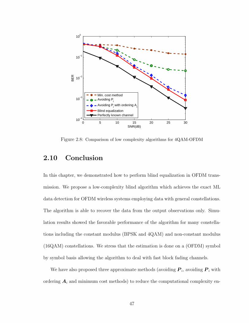
Comparison of low complexity algorithms for 4QAM modulated data

Here, for 4QAM input data (see Figure 2.8), the same conclusion of the BPSK case can

be made, namely, the second method performs quite close to the blind equalization.

43

10 12 14 16 18 20 22 24 26 2810

−3

10−2

10−1

100

SNR(dB)

BE

R

Ch. est. using L+1 pilots and corr.Blind equalizationPerfect known channel

Figure 2.5: BER vs SNR for 16QAM-OFDM over a Rayleigh channel

Comparison of minimum cost method for BPSK modulated data

The minimum cost method described in Section 2.7 was implemented using some

pilots. We give here a simulation result for more realistic OFDM system with N = 64

carriers and 16 Rayleigh fading channel taps. Figure 2.9 shows the performance of

the minimum cost method for the BPSK input data using 12 pilots comparing with

perfectly known channel and pilot based estimation using 12 pilots. It can be seen

that the pilots based method reaches an error floor at high SNR while the minimum

cost method performs better.

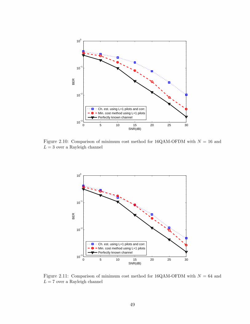
Comparison of minimum cost method for 16QAM modulated data

Figure 2.10 shows the performance of the minimum cost method for the 16QAM

input data with N = 16 carriers and 4 Rayleigh fading channel taps using L+1 pilots

44

0 5 10 15 20 25 3010

−4

10−3

10−2

10−1

100

SNR(dB)

BE

R

Blind equalization (unknown Rh)

Blind equalizationPerfectly known channel

Figure 2.6: BER vs SNR for 4QAM-OFDM without using channel information

comparing with perfectly known channel and pilot based estimation using L+1 pilots.

It can be seen that the minimum cost method improves upon the pilot based channel

estimation method by approximately 5 dB. The same conclusion can be made in Figure

2.11 with 2 dB improvement in the performance at high SNR for 16QAM modulated

data with N = 64 carriers and 8 Rayleigh fading channel taps.

2.9.3 Enhanced Equalization Using Pilots

In the above two subsections, we embed one known data symbol in the OFDM symbol

to resolve the phase ambiguity and to initialize the RLS algorithm used in the blind

equalization. Here, we use some pilots to enhance the equalization. We consider an

OFDM system with N = 16 and L = 3.

45

0 5 10 15 20 25 3010

−4

10−3

10−2

10−1

100

SNR(dB)

BE

R

Min. cost methodAvoiding P

i

Avoiding Pi with ordering A

i

Blind equalizationPerfect known channel

Figure 2.7: Comparison of low complexity algorithms for BPSK-OFDM

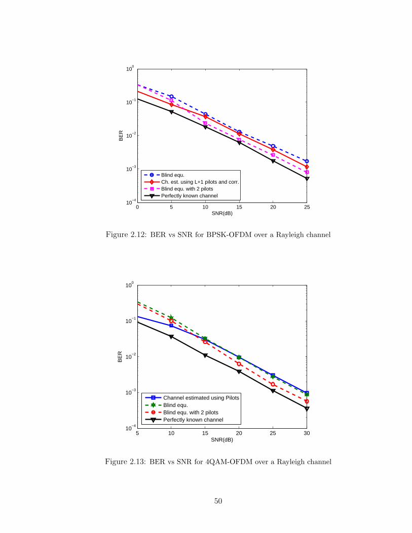
BER vs SNR Comparison for BPSK Modulated Data

Figure 2.12 shows the performance of the receiver with enhanced equalization using

some pilots for BPSK modulated data over a Rayleigh channel. It can be seen that

using of 2 pilots give better performance than the method of channel estimation using

L + 1 pilots and correlation and works very close to the perfectly known channel case

at high SNR.

BER vs SNR Comparison for 4QAM Modulated Data

The performance of the receiver with enhanced equalization using pilots for 4QAM

modulated data is shown in Figure 2.13. Similar to the BPSK modulated data case,

the receiver with 3 pilots shows better BER performance than the method of channel

estimation using pilots.

46

0 5 10 15 20 25 3010

−4

10−3

10−2

10−1

100

SNR(dB)

BE

R

Min. cost methodAvoiding P

i

Avoiding Pi with ordering A

i

Blind equalizationPerfectly known channel

Figure 2.8: Comparison of low complexity algorithms for 4QAM-OFDM

2.10 Conclusion

In this chapter, we demonstrated how to perform blind equalization in OFDM trans-

mission. We propose a low-complexity blind algorithm which achieves the exact ML

data detection for OFDM wireless systems employing data with general constellations.

The algorithm is able to recover the data from the output observations only. Simu-

lation results showed the favorable performance of the algorithm for many constella-

tions including the constant modulus (BPSK and 4QAM) and non-constant modulus

(16QAM) constellations. We stress that the estimation is done on a (OFDM) symbol

by symbol basis allowing the algorithm to deal with fast block fading channels.

We have also proposed three approximate methods (avoiding P i, avoiding P i with

ordering Ai and minimum cost methods) to reduce the computational complexity en-

47

0 5 10 15 20 25 30 35 4010

−5

10−4

10−3

10−2

10−1

100

SNR(dB)

BE

R

Channel est. using 12 pilotsMin. cost method using 12 pilotsPerfectly known channel

Figure 2.9: Comparison of minimum cost method for BPSK-OFDM with N = 64 andL = 15 over a Rayleigh channel

tailed in the algorithm developed in the chapter. It was found that using the second

method performed better than all other methods proposed. We can consider the min-

imum cost method as a pilot based estimation technique which performs better than

the pilot based estimation method. As is evident from the simulation results, some

of these approximate methods perform quite close to the exact blind ML detection

algorithm.

As all standard-based OFDM systems involve some form of training, we have also

studied the behavior of the blind receiver in the presence of pilots.

48

0 5 10 15 20 25 3010

−3

10−2

10−1

100

SNR(dB)

BE

R

Ch. est. using L+1 pilots and corr.Min. cost method using L+1 pilotsPerfectly known channel

Figure 2.10: Comparison of minimum cost method for 16QAM-OFDM with N = 16 andL = 3 over a Rayleigh channel

0 5 10 15 20 25 3010

−3

10−2

10−1

100

SNR(dB)

BE

R

Ch. est. using L+1 pilots and corr.Min. cost method using L+1 pilotsPerfectly known channel

Figure 2.11: Comparison of minimum cost method for 16QAM-OFDM with N = 64 andL = 7 over a Rayleigh channel

49

0 5 10 15 20 2510

−4

10−3

10−2

10−1

100

SNR(dB)

BE

R

Blind equ.Ch. est. using L+1 pilots and corr.Blind equ. with 2 pilotsPerfectly known channel

Figure 2.12: BER vs SNR for BPSK-OFDM over a Rayleigh channel

5 10 15 20 25 3010

−4

10−3

10−2

10−1

100

SNR(dB)

BE

R

Channel estimated using PilotsBlind equ.Blind equ. with 2 pilotsPerfectly known channel

Figure 2.13: BER vs SNR for 4QAM-OFDM over a Rayleigh channel

50

CHAPTER 3

BLIND EQUALIZATION FOR

LINEAR CONVOLUTION SISO

SYSTEMS

3.1 Introduction

The demand for high data rate reliable communications poses great challenges to

the next generation wireless systems in highly dynamic mobile environments. In

this chapter, we investigate the joint Maximum-Likelihood (ML) channel estimation

and signal detection problem for Single-Input Single-Output (SISO) wireless systems

with general modulation constellations and propose an efficient algorithm for finding

the exact joint ML solution. Unlike other known methods, the new algorithm can

even efficiently find the joint ML solution under high spectral efficiency non constant

modulus modulation constellations. In particular, the new algorithm does not need

51

such preprocessing steps as Cholesky or QR decomposition in the traditional sphere

decoders for joint ML channel estimation and data detection.

3.1.1 The Approach and Organization of the Chapter

This chapter considers blind receiver design for SISO transmission over block fading

channels. The receiver employs the maximum likelihood (ML) algorithm for joint

channel and data recovery. It makes collective use of the data and channel constraints

that characterize the communication problem. The data constraints include the fi-

nite alphabet constraint. The channel constraints include the finite delay spread and

frequency and time correlation.

We perform data identification and equalization from output observations only,

without the need for a training sequence or a priori channel information. The advan-

tage of our approach is three fold:

1. The method provides a blind detection of the data from one output data packet

without the need for training.

2. The algorithm works on linear convolution SISO systems employing data with

general constellations.

3. Data equalization is done without any restriction on the channel.

This chapter is organized as follows. We give an overview of the system in Section

3.2. Section 3.3 then presents our approach, while Section 3.4 proposes an algorithm

to reduce the complexity involved in the proposed blind algorithm, while another

52

low complexity equalization method is proposed in section 3.5. We compare the

computational complexities of the various algorithms in Section 3.6, and Section 3.7

shows our simulations. We conclude the chapter in Section 3.8.

3.2 System Overview

Let us consider a SISO system with N be the length of a data packet during which

the channel remains static. Then the channel output is written as

y = h ∗ x∗ + n (3.1)

where h is the channel vector of length L + 1, x∗ is the transmitted symbol sequence

of length N , and n is an additive noise matrix whose elements are assumed to be i.i.d.

complex Gaussian random variables. We also assume that the entries of x∗ are i.i.d.

symbols drawn from a certain constellation Ω (like BPSK or 16-QAM). We can write

(4.1) in matrix form as

y = Xh + n (3.2)

53

where X is the data matrix which has a rectangular Toeplitz structure, i.e., it has

constant entries along its diagonals.

X =

x(1) 0 0 0 · · · 0

x(2) x(1) 0 0 · · · 0

x(3) x(2) x(1) 0 · · · 0

.... . . . . . . . . . . . 0

x(N) x(N − 1) · · · · · · x(N − L + 1) x(N − L)

N×L+1

Note that each row of X amounts to a state vector (also called a regressor) of the

channel. Specifically, the ith row of X has the form

x∗i = [ x(i) x(i− 1) ... x(i− L− 1) ]

which contains the input at time i, x(i), as well as the outputs of all delay elements

in the channel.

3.3 Blind Equalization Approach

The problem of joint ML channel estimation and data detection for SISO channels is

transformed into the following optimization problem

J = minh,x∈ΩN

‖y −Xh‖2 (3.3)

54

where ΩN denotes the set of N -dimensional signal vector.

Let us consider a partial data sequence x∗(i) up to the time index i, i.e.

x∗(i) = [x(1) x(2) · · · x(i)]

Alternatively, we let X(i) denote the matrix that consists of the firsti rows of X, i.e.

X(i) =

x(1) 0 0 · · · 0

x(2) x(1) 0 · · · 0

.... . . . . . . . . 0

x(i) x(i− 1) · · · x(i− L + 1) x(i− L)

Now define Mx∗(i)

to be the cost function associated with the first i data symbols, i.e.

Mx∗(i)

= ‖y(i) −X(i)h‖2 (3.4)

Now, as per Weiyu’s paper [97], let R be the optimal value for our objective

function in (3.3), if Mx∗(i)

> R, then x∗(i) can not be the first i symbols of the ML

solution x∗(i) to (3.3).

To prove this, suppose x∗(i) = x∗(i) and X(i) = X(i), and denote the optimal channel

55

gain corresponding to x∗(i) as h. Then

R = ‖y(i) − X(i)h‖2 +N∑

j=i+1

|y(j)− Xjh|2 (3.5)

≥ minh‖y(i) − X(i)h‖2 +

N∑j=i+1

|y(j)− Xjh|2 (3.6)

≥ minh‖y(i) − X(i)h‖2 = Mx∗

(i)= Mx∗

(i)(3.7)

where Xj corresponding to exactly the Jth row of X.

So, for x(i) to correspond to the first i symbols of the ML solution x(i), we should

have Mx∗(i)

< R. Note that the above represents a necessary condition only in that if

x(i) is such that Mx∗(i)

< R, then that does not necessarily mean that x(i) coincides with

x(i). In the next subsection (3.3.1), we will use this properly in our blind algorithm.

Since h has L + 1 degrees of freedom, so we need L + 1 pilots to identify it.

Alternatively, we need to make a guess of L+1 consecutive values of the input before

we get a unique solution for h. In otherwords, with i < L + 1, it is always possible to

choose X i and h so that the cost function in (3.4) is identically zero. This does not

allow us to refine our search to obtain the most suitable data sequence.

To avoid this problem, we replace the cost function in (3.3) with the regularized

least squares problem

J = minh,x∈ΩN

‖h‖2R−1

h+ ‖y −Xh‖2

Rn−1 (3.8)

where Rh is the autocorrelation matrix of h and Rn is the noise autocorrelation

matrix, given by σ2I where σ2 is the noise variance. In this case, we can show that

56

Mx∗(i)

is given by

Mx∗(i)

= ‖h‖2R−1

h+ ‖y(i) −X(i)h‖2

Rn−1 (3.9)

= y∗(i)[Rn + X∗(i)RhX(i)]

−1y(i) (3.10)

This solution is computationally complex as it use the matrix inversion lemma. So,

we can recursively calculate the value of the objective function (Mx∗(i)

) for each i using

the RLS algorithm through the following set of recursions

Mx∗(i)

= Mx∗(i−1)

+ 1σ2 γ(i)|y(i)− x∗i hi−1|2 (3.11)

where

hi = hi−1 + 1σgi(y(i)− x∗i hi−1) (3.12)

and

gi =1

σγ(i)P i−1xi (3.13)

γ(i) =1

1 + 1σ2 x∗i P i−1xi

(3.14)

P i = P i−1 − (gig∗i )/γ(i) (3.15)

= P i−1 − 1

σ2γ(i)P i−1xix

∗i P i−1 (3.16)

57

These recursions apply for all i and are initialized by

Mx∗(−1)

= 0, P−1 = Rh, and h−1 = 0

Now, R is the optimal value for the regularized objective function in (3.8), and

Mx∗(i)

is the value of the objective function in (3.11) for the sequence x∗(i) up to the time

index i. If the value R can be estimated, we can restrict the search of the blind ML

solution x∗ to the offsprings of those partial sequences x∗(i) which satisfy Mx∗(i)

< R.

3.3.1 Exact Blind Algorithm

In this section, we describe the algorithm that we use to find the ML solution of the

system input from the output observations. The algorithm employs the above set of

iterations (3.11)−(3.16) to update the value of the cost function (Mx∗(i)

) which we need

for the comparison with the estimated value R (we denote it in the blind algorithm

below as the search radius r).

The input parameters for this algorithm are:

• The received channel output y

• The search radius r

• The modulation constellation Ω

• 1×N index vector I

We denote the kth constellation point in the modulation constellation Ω as Ω(k).

58

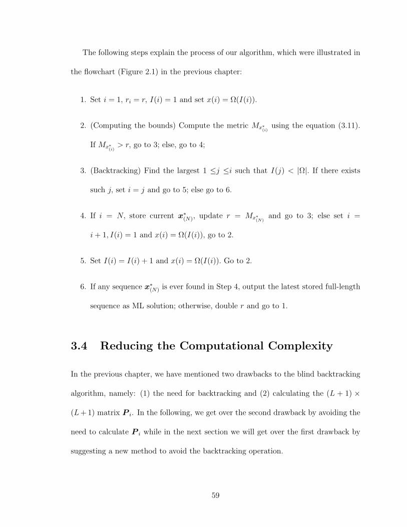
The following steps explain the process of our algorithm, which were illustrated in

the flowchart (Figure 2.1) in the previous chapter:

1. Set i = 1, ri = r, I(i) = 1 and set x(i) = Ω(I(i)).

2. (Computing the bounds) Compute the metric Mx∗(i)

using the equation (3.11).

If Mx∗(i)

> r, go to 3; else, go to 4;

3. (Backtracking) Find the largest 1 ≤j ≤i such that I(j) < |Ω|. If there exists

such j, set i = j and go to 5; else go to 6.

4. If i = N, store current x∗(N), update r = Mx∗(N)

and go to 3; else set i =

i + 1, I(i) = 1 and x(i) = Ω(I(i)), go to 2.

5. Set I(i) = I(i) + 1 and x(i) = Ω(I(i)). Go to 2.

6. If any sequence x∗(N) is ever found in Step 4, output the latest stored full-length

sequence as ML solution; otherwise, double r and go to 1.

3.4 Reducing the Computational Complexity

In the previous chapter, we have mentioned two drawbacks to the blind backtracking

algorithm, namely: (1) the need for backtracking and (2) calculating the (L + 1) ×

(L + 1) matrix P i. In the following, we get over the second drawback by avoiding the

need to calculate P i while in the next section we will get over the first drawback by

suggesting a new method to avoid the backtracking operation.

59

The RLS algorithm that we have used above is not assume any structure in the

data. So, the computational complexity of this algorithm is O((L + 1)2) operations

per iteration (see table 3.1), where L + 1 is the channel length. However, when data

structure is present, more efficient implementations are possible.

In our case (Linear systems), the regressors x∗i exhibit some form of structure

which arise as regressors of a tapped-delay-line implementation. That is, we can see

that the entries of x∗i are formed from time-delayed samples of an input sequence x(.),

say,

x∗i = [ x(i) x(i− 1) ... x(i− L− 1) ]

The shift structure in the regressors allows us to utilize an efficient recursive least-

squares solutions, which is the Fast RLS Array Algorithm. By efficient we mean

its computational complexity is O(L + 1) operations per iteration, as opposed to

O((L + 1)2).

So, we can recursively calculate the value of the objective function in (3.9) (repro-

duced here for convenience)

Mx∗(i)

= ‖h‖2R−1

h+ ‖y(i) −X(i)h‖2

Rn−1 (3.17)

for each i using the Fast RLS array algorithm through the following set of recursions

initialized by

Mx∗(−1)

= 0, g−1 = 0, γ−1/2(−1) = 1, h−1 = 0,

60

L−1 =√

ηλ

1 0

0 0

......

0 0

0 λ(L+1)/2

, S−1 =

1 0

0 −1

and l = diag(1,S)

where L−1 is ((L + 2)× 2) matrix and S−1 is (2× 2) signature matrix.

1. Find the l−unitary matrix Θi that annihilates the last two entries in the top row

of the post-array below and generates a positive leading entry. The l−unitary

matrix Θ should satisfy

Θ

1

S

Θ∗ =

1

S

Then the entries of the post-array will correspond to

γ−1/2(i− 1) [x(i) xi−1] Li−1

0

gi−1γ−1/2(i− 1)

Li−1

Θi

=

γ−1/2(i) [0 0]

giγ−1/2(i)

0

√λLi

61

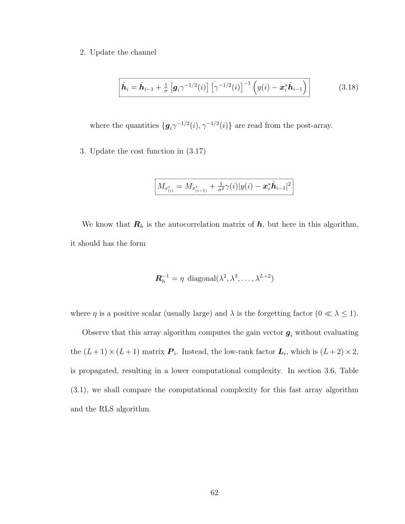
2. Update the channel

hi = hi−1 + 1σ

[giγ

−1/2(i)] [

γ−1/2(i)]−1

(y(i)− x∗i hi−1

)(3.18)

where the quantities giγ−1/2(i), γ−1/2(i) are read from the post-array.

3. Update the cost function in (3.17)

Mx∗(i)

= Mx∗(i−1)

+ 1σ2 γ(i)|y(i)− x∗i hi−1|2

We know that Rh is the autocorrelation matrix of h, but here in this algorithm,

it should has the form

R−1h = η diagonal(λ2, λ3, . . . , λL+2)

where η is a positive scalar (usually large) and λ is the forgetting factor (0 ¿ λ ≤ 1).

Observe that this array algorithm computes the gain vector gi without evaluating

the (L+1)× (L+1) matrix P i. Instead, the low-rank factor Li, which is (L+2)× 2,

is propagated, resulting in a lower computational complexity. In section 3.6, Table

(3.1), we shall compare the computational complexity for this fast array algorithm

and the RLS algorithm.

62

3.5 Minimum Cost Method

In the previous section, we showed how to avoid the need for calculating P i by using

the Fast RLS algorithm. In this section, we propose a new method to avoid the

backtracking operation in the blind algorithm and give a very low complexity.

Our objective in data detection is to minimize the cost function. In this method,

we depend on finding the constellation points that minimize the cost function at each

data symbol (according to the following equation (3.19)) and take them as a solution

without the need for backtracking.

From (3.11), and for the j-th constellation point (Ω(j)), we can define M jx∗(i)

as the

cost function up to the time index i, say

M jx∗(i)

= Mx∗(i−1)

+ 1σ2 γ(i)|y(i)− Ω(j)hi−1|2 (3.19)

After we compute all the j values of the cost function using the above equation, we

find the minimum one and its index (l), then store the l-th constellation point in the

i-th solution x(i). The same procedure is followed for the next symbol up to the one

at time N .

In this method, there is no need to do backtracking, which gives us a very low

complexity compared with the backtracking method in Section 3.3.1, but this method

needs to have some pilots to give good results as we shall show in the simulation

results.

In addition, this method can be also used as an equalization method when the

63

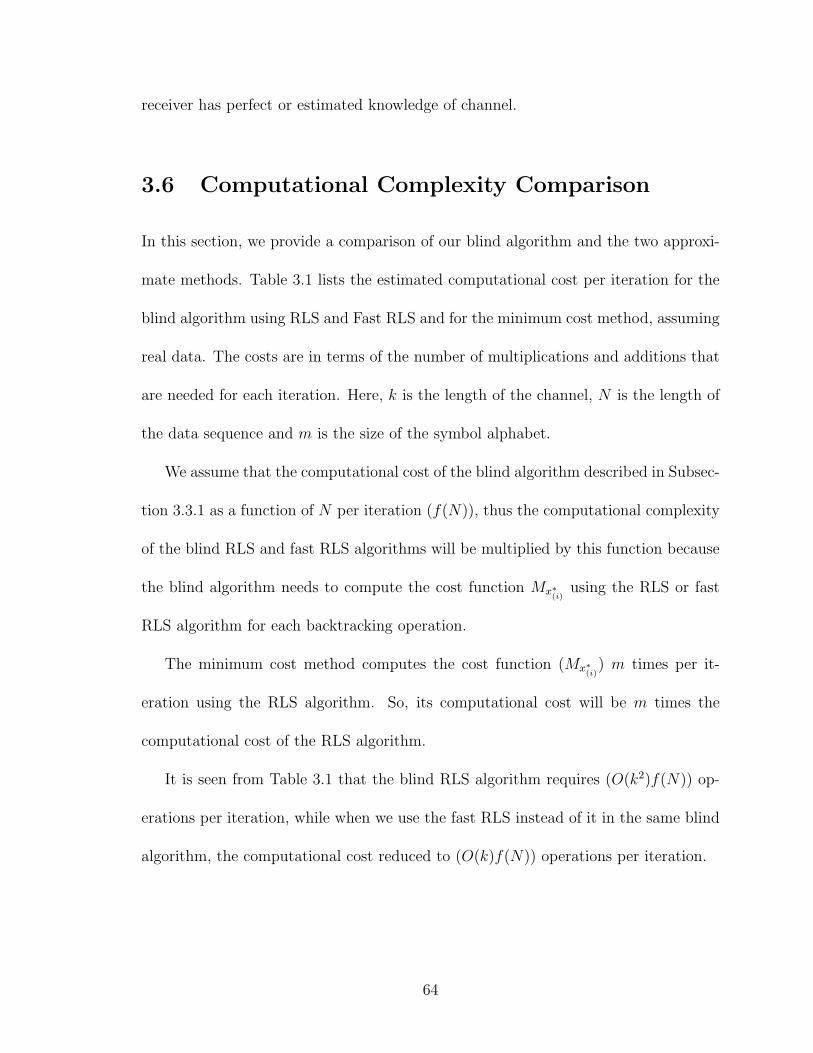
receiver has perfect or estimated knowledge of channel.

3.6 Computational Complexity Comparison

In this section, we provide a comparison of our blind algorithm and the two approxi-

mate methods. Table 3.1 lists the estimated computational cost per iteration for the

blind algorithm using RLS and Fast RLS and for the minimum cost method, assuming

real data. The costs are in terms of the number of multiplications and additions that

are needed for each iteration. Here, k is the length of the channel, N is the length of

the data sequence and m is the size of the symbol alphabet.

We assume that the computational cost of the blind algorithm described in Subsec-

tion 3.3.1 as a function of N per iteration (f(N)), thus the computational complexity

of the blind RLS and fast RLS algorithms will be multiplied by this function because

the blind algorithm needs to compute the cost function Mx∗(i)

using the RLS or fast

RLS algorithm for each backtracking operation.

The minimum cost method computes the cost function (Mx∗(i)

) m times per it-

eration using the RLS algorithm. So, its computational cost will be m times the

computational cost of the RLS algorithm.

It is seen from Table 3.1 that the blind RLS algorithm requires (O(k2)f(N)) op-

erations per iteration, while when we use the fast RLS instead of it in the same blind

algorithm, the computational cost reduced to (O(k)f(N)) operations per iteration.

64

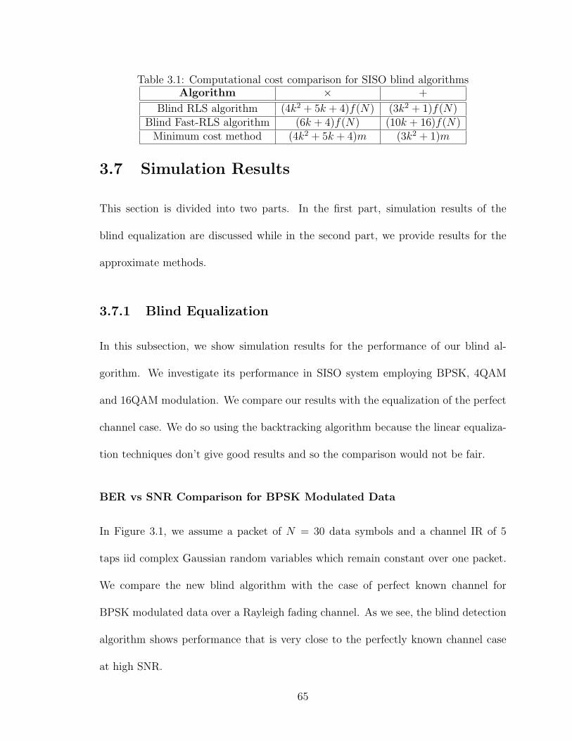
Table 3.1: Computational cost comparison for SISO blind algorithmsAlgorithm × +

Blind RLS algorithm (4k2 + 5k + 4)f(N) (3k2 + 1)f(N)Blind Fast-RLS algorithm (6k + 4)f(N) (10k + 16)f(N)

Minimum cost method (4k2 + 5k + 4)m (3k2 + 1)m

3.7 Simulation Results

This section is divided into two parts. In the first part, simulation results of the

blind equalization are discussed while in the second part, we provide results for the

approximate methods.

3.7.1 Blind Equalization

In this subsection, we show simulation results for the performance of our blind al-

gorithm. We investigate its performance in SISO system employing BPSK, 4QAM

and 16QAM modulation. We compare our results with the equalization of the perfect

channel case. We do so using the backtracking algorithm because the linear equaliza-

tion techniques don’t give good results and so the comparison would not be fair.

BER vs SNR Comparison for BPSK Modulated Data

In Figure 3.1, we assume a packet of N = 30 data symbols and a channel IR of 5

taps iid complex Gaussian random variables which remain constant over one packet.

We compare the new blind algorithm with the case of perfect known channel for

BPSK modulated data over a Rayleigh fading channel. As we see, the blind detection

algorithm shows performance that is very close to the perfectly known channel case

at high SNR.

65

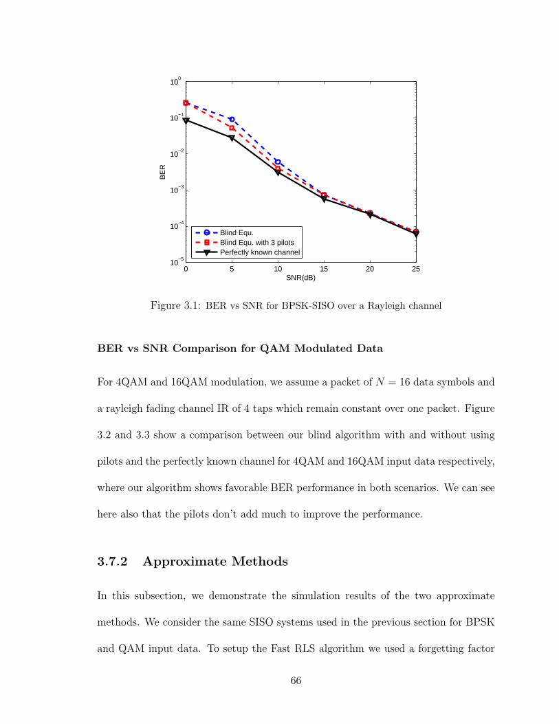
0 5 10 15 20 2510

−5

10−4

10−3

10−2

10−1

100

SNR(dB)

BE

R

Blind Equ.Blind Equ. with 3 pilotsPerfectly known channel

Figure 3.1: BER vs SNR for BPSK-SISO over a Rayleigh channel

BER vs SNR Comparison for QAM Modulated Data

For 4QAM and 16QAM modulation, we assume a packet of N = 16 data symbols and

a rayleigh fading channel IR of 4 taps which remain constant over one packet. Figure

3.2 and 3.3 show a comparison between our blind algorithm with and without using

pilots and the perfectly known channel for 4QAM and 16QAM input data respectively,

where our algorithm shows favorable BER performance in both scenarios. We can see

here also that the pilots don’t add much to improve the performance.

3.7.2 Approximate Methods

In this subsection, we demonstrate the simulation results of the two approximate

methods. We consider the same SISO systems used in the previous section for BPSK

and QAM input data. To setup the Fast RLS algorithm we used a forgetting factor

66

5 10 15 20 25 3010

−5

10−4

10−3

10−2

10−1

100

Blind Equ.Blind Equ. with L+1 pilotsPerfectly known channel

Figure 3.2: BER vs SNR for 4QAM-SISO over a Rayleigh channel

of λ = 0.999 and η = 5.

Performance of low complexity algorithms for BPSK Modulated Data

Figure 3.4 shows the BER performance comparison between the backtracking method

and the low computational complexity method (Fast RLS algorithm), for BPSK input

data. As we see the method of low complexity performs very close to the blind RLS

method.

Performance of low complexity algorithms for 4QAM Modulated Data

The BER performance of the backtracking method and the low computational com-

plexity method is given in Figure 3.5, for 4QAM input data. Our conclusion is similar

to the conclusion in the BPSK case, namely, the Fast RLS algorithm performs very

67

5 10 15 20 25 3010

−4

10−3

10−2

10−1

100

SNR(dB)

BE

R

Blind Equ.Blind Equ. with L+1 pilotsPerfectly known channel

Figure 3.3: BER vs SNR for 16QAM-SISO over a Rayleigh channel

closely to the performance of the RLS backtracking method.

Performance of the minimum cost method for BPSK Modulated Data

In Figure 3.6, we show the performance of the minimum cost method for BPSK input

data with N = 30 over 5 Rayleigh fading channel taps. We investigate its performance

for three cases; using one training symbol, using L + 1 pilots and using the perfectly

known channel. The case of perfectly known channel gives, as expected, the best

performance. Therefore, we conclude that the minimum cost method is best suited

for the equalization of perfectly known channel.

68

5 10 15 20 2510

−5

10−4

10−3

10−2

10−1

SNR(dB)

BE

R

Approx. method (Fast RLS)Blind Equ.Perfectly known channel

Figure 3.4: Performance of low complexity algorithm for BPSK-SISO

Performance of minimum cost method for QAM Modulated Data

Figure 3.7 and 3.8, show the performance of the minimum cost method for 4QAM

and 16QAM input data, respectively, with N = 16 over a Rayleigh fading channel

with 4 taps. The same conclusion of BPSK case can be made here, namely, that the

minimum cost method is best suited for equalization of perfectly known channel.

3.8 Conclusion

In this chapter, we proposed a new blind algorithm for data detection in SISO wireless

systems employing data with general constellation. The algorithm is able to recover

the data from the output observations only. Simulation results showed the favorable

performance of the algorithm for several constellations (BPSK, 4QAM and 16QAM).

69

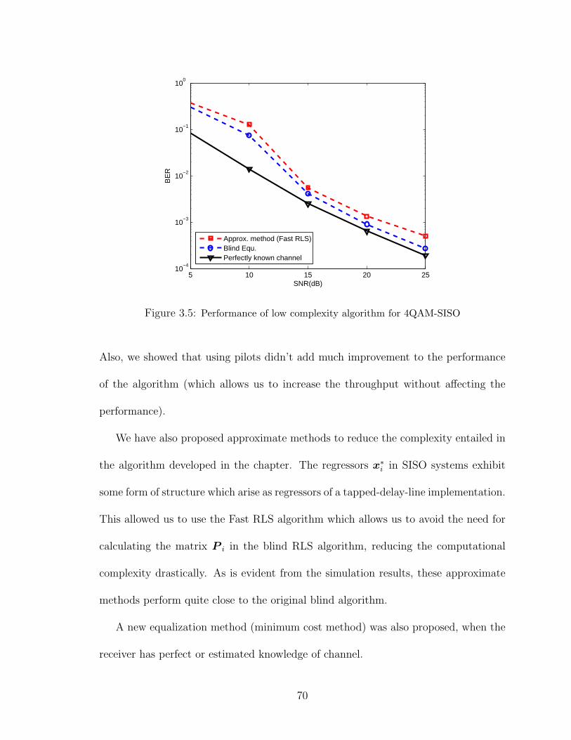
5 10 15 20 2510

−4

10−3

10−2

10−1

100

SNR(dB)

BE

R

Approx. method (Fast RLS)Blind Equ.Perfectly known channel

Figure 3.5: Performance of low complexity algorithm for 4QAM-SISO

Also, we showed that using pilots didn’t add much improvement to the performance

of the algorithm (which allows us to increase the throughput without affecting the

performance).

We have also proposed approximate methods to reduce the complexity entailed in

the algorithm developed in the chapter. The regressors x∗i in SISO systems exhibit

some form of structure which arise as regressors of a tapped-delay-line implementation.

This allowed us to use the Fast RLS algorithm which allows us to avoid the need for

calculating the matrix P i in the blind RLS algorithm, reducing the computational

complexity drastically. As is evident from the simulation results, these approximate

methods perform quite close to the original blind algorithm.

A new equalization method (minimum cost method) was also proposed, when the

receiver has perfect or estimated knowledge of channel.

70

0 5 10 15 20 25 30 3510

−4

10−3

10−2

10−1

100

SNR(dB)

BE

R

Min. cost method using 1 pilotMin. cost method using L+1 pilotsMin. cost method with perfectly known channel

Figure 3.6: Performance of minimum cost method for BPSK-SISO over a Rayleigh channel

0 5 10 15 20 25 30 3510

−4

10−3

10−2

10−1

100

SNR(dB)

BE

R

Min. cost method using 1 pilotMin. cost method using L+1 pilotsMin. cost method using perfectly known channel

Figure 3.7: Performance of minimum cost method for 4QAM-SISO over a Rayleigh channel

71

0 5 10 15 20 25 30 3510

−3

10−2

10−1

100

SNR(dB)

BE

R

Min. cost method using 1 pilotMin. cost method using L+1 pilotsMin. cost method using perfectly known channel

Figure 3.8: Performance of minimum cost method for 16QAM-SISO over a Rayleigh channel

72

CHAPTER 4

SISO SYSTEMS OVER

TIME-VARIANT CHANNELS

4.1 Introduction

The goal of achieving high-speed reliable data transmission over highly dynamic wire-

less medium has generated a lot of research activities in the communications and signal

processing community. One of the largest challenges arising in wireless communica-

tions is how to deal with the wireless fading phenomenon, where the wireless channels

may vary over time. In wireless communications, one often assumes knowledge of the

channel coefficients at the receiver side by channel estimation from training sequences,

but sending training symbols will sacrifice a fraction of the transmission rate. In wire-

less mobile systems, the channels may even change so rapidly that training and channel

tracking will become infeasible. One possible solution is to differentially encode the

transmitted data and thus eliminate the need for channel knowledge. Another solution

73

is to do blind or semi-blind detection over the time-varying wireless channels, which

has been shown to enhance the system performance considerably and often perform

better than differential modulations.

In this chapter, we consider the problem of joint maximum likelihood (ML) channel

estimation and data detection for linear convolution SISO systems over time-variant

channels.

4.1.1 The Approach and Organization of this Chapter

This chapter considers blind receiver design for linear convolution SISO transmission

over frequency selective time-variant channels. The receiver employs the ML algorithm

for joint channel and data recovery. It makes collective use of the data and channel

constraints that characterize the communication problem. The data constraints in-

clude the finite alphabet constraint. The channel constraints include the finite delay

spread and frequency and time correlation.

We perform data identification and equalization from output observations only,

without the need for a training sequence or a priori channel information. The advan-

tage of our approach is three fold:

1. The method provides a blind detection of the data from one output data packet

without the need for training.

2. The algorithm works on linear convolution SISO systems employing data with

general constellations.

74

3. The algorithm works on linear convolution SISO systems over time-variant chan-

nel without any restriction.

This chapter is organized as follows. We give a description of the channel model

in Section 4.2. Section 4.3 then presents our approach, and Section 4.4 demonstrates

our simulations. We conclude the chapter in Section 4.5.

4.2 Channel Model

In the previous chapter, we have described our algorithm using block fading channels,

which showed a favorable results. In this chapter, we peruse the same backtracking

algorithm in time variant channels.

Let us consider the same SISO system in the previous chapter, where the in-

put/output relationship can be written as

y = h ∗ x∗ + n (4.1)

= Xh + n (4.2)

except that the channel vector h of length L + 1 varies here from one symbol to the

next according to the following state space model

hi+1 = Fhi + Gui (4.3)

where h0 ∼ N (0, R) and ui ∼ N (0, σ2uI). The matrices F and G in (4.3) are square

75

matrices of size L + 1 and are function of Doppler spread, power delay profile and

transmit filter, and they are given by

F =

α(0)

α(1)

. . .

α(L)

and

G =

√1− α2(0)

√(1− α2(1))e−β(1)

. . .

√(1− α2(L))e−βL

where α(l) is related to the Doppler frequency fD(l) by α(l) = J0(2πfD(l)T ), where J0

denotes the zero-order Bessel function of the first kind and T is the symbol time. The

variable β corresponds to the exponent of the channel decay profile while the factor

√(1− α2(l))e−βl ensures that each link maintains the exponential decay profile (e−βl)

for all time.

The Doppler frequency fD(l) is related to the vehicle speed v(l) and the wavelength

λ = cf

by fD(l) = v(l)λ

, where c is the speed of light and f is the transmission frequency.

In our simulations, we consider constant vehicle speed, i.e. v(l) = v, thus the time

76

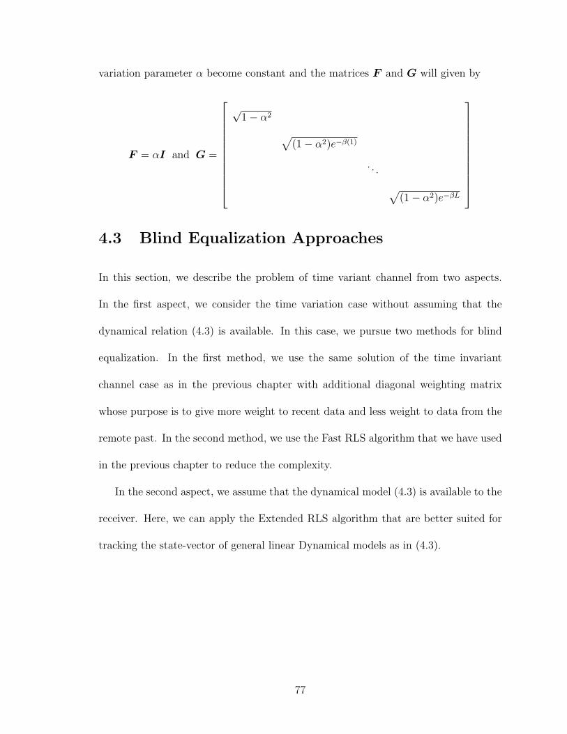
variation parameter α become constant and the matrices F and G will given by

F = αI and G =

√1− α2

√(1− α2)e−β(1)

. . .

√(1− α2)e−βL

4.3 Blind Equalization Approaches

In this section, we describe the problem of time variant channel from two aspects.

In the first aspect, we consider the time variation case without assuming that the

dynamical relation (4.3) is available. In this case, we pursue two methods for blind

equalization. In the first method, we use the same solution of the time invariant

channel case as in the previous chapter with additional diagonal weighting matrix

whose purpose is to give more weight to recent data and less weight to data from the

remote past. In the second method, we use the Fast RLS algorithm that we have used

in the previous chapter to reduce the complexity.

In the second aspect, we assume that the dynamical model (4.3) is available to the

receiver. Here, we can apply the Extended RLS algorithm that are better suited for

tracking the state-vector of general linear Dynamical models as in (4.3).

77

4.3.1 Blind Equalization Without Knowledge of the Chan-

nel’s Dynamical Model

In this subsection, we consider the case of no knowledge of the matrices F and G in

the dynamical model (4.3) are available at the receiver. We pursue here two methods

for blind equalization described below.

Exponentially-Weighted RLS Approach

In our first approach, we use an Exponentially-Weighted RLS algorithm. Here, we em-

ploy a weighted regularized least-squares cost function, as opposed to the unweighted

cost in (3.8). Namely, replace the cost function in (3.8) by

J = minh,x∈ΩN

[‖h‖2

λNR−1h

+ ‖y −Xh‖2Λ−1

](4.4)

where 0 ¿ λ < 1 is a positive scalar, usually very close to one, and introduce the

diagonal matrix

Λ = diagλN−1, λN−2, . . . , λ, 1

The scalar λ is called the forgetting factor since past data are weighted less heavily

than more recent data. The special case λ = 1 is known as the growing memory case

and it was studied in the previous chapter.

Observe that the regularization matrix in (4.4) is chosen as λNR−1h , with the

additional scaling factor λN . Since this factor becomes smaller as time progresses, we

see that the exponentially-weighted cost function (4.4) is such that it de-emphasizes

78

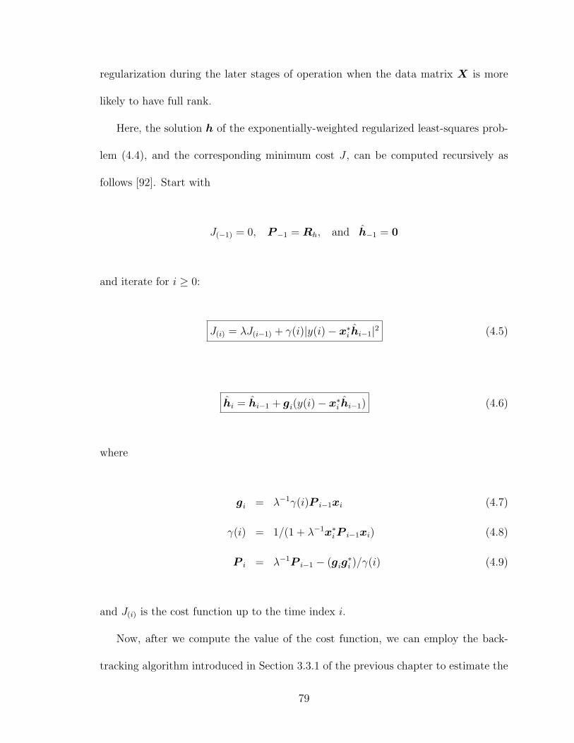
regularization during the later stages of operation when the data matrix X is more

likely to have full rank.

Here, the solution h of the exponentially-weighted regularized least-squares prob-

lem (4.4), and the corresponding minimum cost J , can be computed recursively as

follows [92]. Start with

J(−1) = 0, P−1 = Rh, and h−1 = 0

and iterate for i ≥ 0:

J(i) = λJ(i−1) + γ(i)|y(i)− x∗i hi−1|2 (4.5)

hi = hi−1 + gi(y(i)− x∗i hi−1) (4.6)

where

gi = λ−1γ(i)P i−1xi (4.7)

γ(i) = 1/(1 + λ−1x∗i P i−1xi) (4.8)

P i = λ−1P i−1 − (gig∗i )/γ(i) (4.9)

and J(i) is the cost function up to the time index i.

Now, after we compute the value of the cost function, we can employ the back-

tracking algorithm introduced in Section 3.3.1 of the previous chapter to estimate the

79

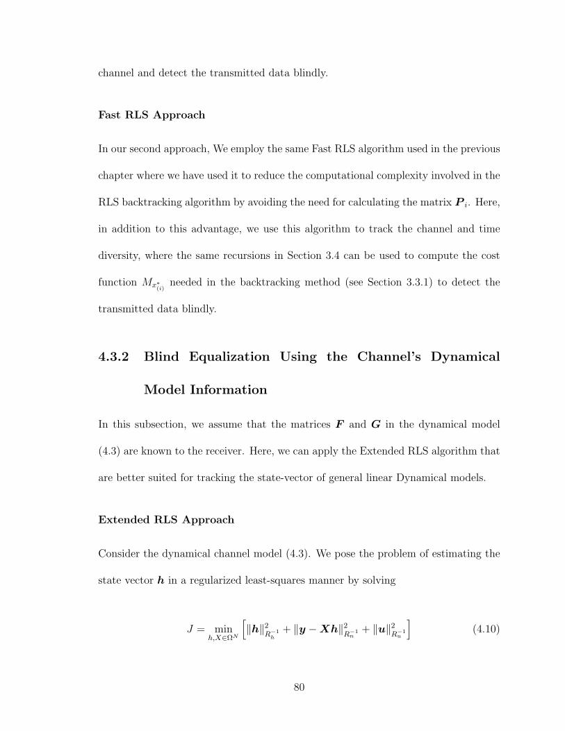
channel and detect the transmitted data blindly.

Fast RLS Approach

In our second approach, We employ the same Fast RLS algorithm used in the previous

chapter where we have used it to reduce the computational complexity involved in the

RLS backtracking algorithm by avoiding the need for calculating the matrix P i. Here,

in addition to this advantage, we use this algorithm to track the channel and time

diversity, where the same recursions in Section 3.4 can be used to compute the cost

function Mx∗(i)

needed in the backtracking method (see Section 3.3.1) to detect the

transmitted data blindly.

4.3.2 Blind Equalization Using the Channel’s Dynamical

Model Information

In this subsection, we assume that the matrices F and G in the dynamical model

(4.3) are known to the receiver. Here, we can apply the Extended RLS algorithm that

are better suited for tracking the state-vector of general linear Dynamical models.

Extended RLS Approach

Consider the dynamical channel model (4.3). We pose the problem of estimating the

state vector h in a regularized least-squares manner by solving

J = minh,X∈ΩN

[‖h‖2

R−1h

+ ‖y −Xh‖2R−1

n+ ‖u‖2

R−1u

](4.10)

80

where Ru and Rn are positive-definite weighting matrices that could be taken as the

covariance matrices of the noises u (i.e. σ2uI) and n (i.e. σ2

nI), respectively.

The solution h and the cost function J can be determined recursively as follows

[92]. Start with

J(−1) = 0, P−1 = Rh, and h−1 = 0

and run the following equations for i ≥ 0:

J(i) = J(i−1) + γ(i)−1|y(i)− x∗i hi−1|2 (4.11)

hi = F hi−1 + gi(y(i)− x∗i hi−1) (4.12)

where

gi = γ(i)−1FP i−1xi (4.13)

γ(i) = σ2n + x∗i P i−1xi (4.14)

P i = FP i−1F∗ + GRuG

∗ − γ(i)gig∗i (4.15)

and J(i) is the cost function up to the time index i,

Here, we can also employ the backtracking algorithm introduced in Section (3.3.1)

in the previous chapter to estimate the channel and detect the transmitted data

blindly.

81

Table 4.1: Simulation and fading channel parametersParameter Value

Packet length(N) 16Channel length(L + 1) 4Transmission frequency 2 GHz

Vehicle speed 50 and 200 km/hrSymbol period 20 µs

Forgetting factor (λ) 0.999Exponent of the channel decay profile (β) 0.2

The F-RLS parameter (η) 5

4.4 Simulation Results

In this section, we show simulation results for the performance of our blind equal-

ization using Exponentially-Weighting RLS (EW-RLS), Extended RLS (E-RLS), and

Fast RLS (F-RLS) algorithms. We investigate its performance in SISO system employ-

ing BPSK, 4QAM and 16QAM modulation over time variant channel IR generated

according to the dynamical model in (4.3). We also study the effect of the time vari-

ation degree on the performance of the three methods. The parameters used in the

simulation and generating the fading channel are shown in Table 4.1.

4.4.1 Performance of the three RLS algorithms

Here, we show simulation results for the performance of our blind algorithm using

the three methods. We investigate its performance in SISO system employing BPSK,

4QAM and 16QAM modulation over time variant channel IR generated according to

the dynamical model in (4.3) with α = 0.99995 for a vehicle speed of 50 km/hr.

82

BER performance for BPSK modulated data

In Figures 4.1 and 4.2, we compare the new blind algorithm for BPSK modulated

data over time variant channel using the three methods with α = 0.99995 and 0.9951

respectively. We compare them also with the case of time invariant channel. As we see

in Figure 4.1, the three methods work very close to the time invariant channel at low

vehicle speed (50 km/hr corresponds to α = 0.99995) while at high speed (200 km/hr

corresponds to α = 0.99951) only the F-RLS algorithm works better (see Figure 4.2).

5 10 15 20 2510

−4

10−3

10−2

10−1

100

SNR(dB)

BE

R

Blind equ. using EW−RLSBlind equ. using E−RLSBlind equ. using F−RLSBlind equ. timeInvar.

Figure 4.1: BER vs SNR for BPSK-SISO over time variant channel at low vehicle speed

BER performance for 4QAM modulated data

The same conclusion can be made for 4QAM modulation at high vehicle speed (200

km/hr corresponds to α = 0.99951)(see Figure 4.3), where F-RLS algorithm shows

83

5 10 15 20 2510

−4

10−3

10−2

10−1

100

SNR(dB)

BE

R

Blind equ. using EW−RLSBlind equ. using E−RLSBlind equ. using F−RLSBlind equ. timeInvar.

Figure 4.2: BER vs SNR for BPSK-SISO over time variant channel at high vehicle speed

favorable BER performance.

4.4.2 Effect of time variation

In this subsection, we test the performance of our receiver against different degrees

of time variation. This is parameterized by α (0 ≤ α ≤ 1) with lower values of

α indicating a faster time-variant channel. According to Table 4.1, the range of α

is 99951 to 0.99995 for a vehicle speed decreasing from 200 km/hr to 50 km/hr,

respectively.

For comparison, In Figures 4.4, 4.5, and 4.6, we show the BER curves for a system

that employs BPSK data using the three methods EW-RLS, E-RLS and F-RLS to

test its robustness against the time variation. It can be seen that the third method in

Figure 4.6 has the best robust behavior when we change the time variant parameter

84

5 10 15 20 2510

−4

10−3

10−2

10−1

100

Blind equ. using EW−RLSBlind equ. using E−RLSBlind equ. using F−RLSBlind equ. timeInvar.

Figure 4.3: BER vs SNR for 4QAM-SISO over time variant channel at high vehicle speed

α from 0.99995 to 0.99951. Therefore, we are able to track the channel and capture

time diversity at high vehicle speed.

4.5 Conclusion

In this chapter, we presented a blind algorithm for channel estimation and data re-

covery in linear convolution SISO transmission over frequency selective time-variant

channels, where it varies form one data symbol to the next according to dynamical

model. Three modification/extensions of the RLS algorithm were employed by the

new blind algorithm which include the exponentially weighted RLS, the Fast RLS and

the Extended RLS algorithm. The performance of the receiver by employing the three

different implementations of the RLS was presented. Simulation results showed that

85

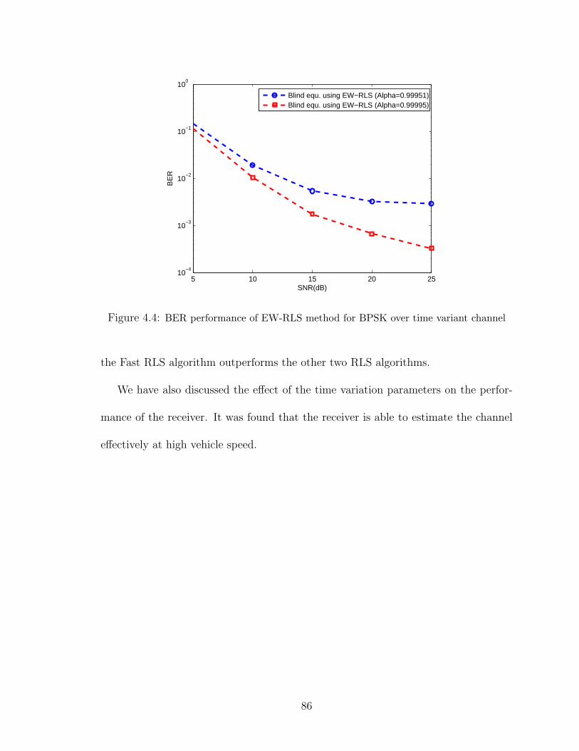
5 10 15 20 2510

−4

10−3

10−2

10−1

100

SNR(dB)

BE

R

Blind equ. using EW−RLS (Alpha=0.99951)Blind equ. using EW−RLS (Alpha=0.99995)

Figure 4.4: BER performance of EW-RLS method for BPSK over time variant channel

the Fast RLS algorithm outperforms the other two RLS algorithms.

We have also discussed the effect of the time variation parameters on the perfor-

mance of the receiver. It was found that the receiver is able to estimate the channel

effectively at high vehicle speed.

86

5 10 15 20 25 3010

−4

10−3

10−2

10−1

100

SNR(dB)

BE

R

Blind equ. using E−RLS (Alpha=0.99951)Blind equ. using E−RLS (Alpha=0.99995)

Figure 4.5: BER performance of E-RLS method for BPSK over time variant channel

5 10 15 20 2510

−4

10−3

10−2

10−1

100

SNR(dB)

BE

R

Blind equ. using F−RLS (Alpha=.99951)Blind equ. using F−RLS (Alpha=.99995)

Figure 4.6: BER performance of F-RLS method for BPSK over time variant channel

87

CHAPTER 5

CONCLUSIONS AND FUTURE

WORK

5.1 Concluding Remarks

This Thesis has considered blind algorithms for channel estimation and data recovery

in SISO transmission. The first part of the Thesis presented a new blind algorithm

for circular convolution SISO systems. We propose a low-complexity blind algorithm

which achieves the exact ML data detection for OFDM wireless systems employing

data with general constellations. The algorithm is able to recover the data from the

output observations only. Simulation results showed the favorable performance of the

algorithm for many constellations including the constant modulus (BPSK and 4QAM)

and non-constant modulus (16QAM) constellations. To reduce the computational

complexity involved in the blind algorithm, three methods were proposed; avoiding

P i, avoiding P i with ordering Ai and minimum cost methods. It was found that

88

using the second method performed better than all other methods proposed. We can

consider the minimum cost method as a pilot based estimation technique. Specifically,

in this method, data is recovered by finding the constellation point that minimizing

the cost function without backtracking giving a very low complexity.

The second part of Thesis presented the new blind algorithm for data detection in

linear convolution SISO wireless systems employing data with general constellations.

Simulation results showed the favorable performance of the algorithm for many con-

stellations. It was found that using some pilots didn’t add much improvement to the

performance of the algorithm. We have also proposed approximate methods to reduce

the complexity entailed in the blind algorithm. The structure of the regressors in the

linear convolution SISO systems allowed us to use the Fast RLS algorithm which avoid

the need for calculating the matrix P i in the blind RLS algorithm and thus give lower

complexity. As is evident from the simulation results, this approximate method per-

form quite close to the blind algorithm. A new equalization method (minimum cost

method) was also proposed, when the receiver has perfect or estimated knowledge of

channel.

The last part of Thesis considered a blind receiver design for linear convolution

SISO transmission over time-variant channels. Some possible constraints on the chan-

nel (the finite delay spread, frequency and time correlation) and the data (the finite al-

phabet constraint) were utilized. Three modification/extensions of the RLS algorithm

were employed by the new blind algorithm which include the Exponentially-Weighted

RLS, Fast RLS and Extended RLS algorithms. The simulation results showed that

89

the Fast RLS algorithm outperforms the other two RLS algorithms. We have also dis-

cussed the effect of the time variation parameters on the performance of the receiver,

where the Fast RLS algorithm showed better robustness against the changing of the

time variation parameters.

5.2 Future Work

5.2.1 General Time Variant Case for OFDM System

This Thesis deals with block fading channels in OFDM system (Chapter 2) i.e. the

channel is assumed to be constant during the transmission of one OFDM symbol.

It is more realistic to assume that the channel continuously varies with time which

is a future research problem which can be build upon the findings in this Thesis.

Specifically, we will assume that the channel varies within the OFDM symbol (resulting

in intercarrier interference (ICI)) and use the various constraints used in this Thesis

to perform channel estimation, ICI cancelation, and data detection.

5.2.2 Motivating the Constant Modulus Algorithm

Constant modulus algorithm (CMA) is a blind equalization method that uses the out-

put observations only to detects the data without the need for any training sequence.

Our blind algorithm does the same thing except that the CMA needs some time to

converge while our algorithm can detects the data from the fist packet. So, with some

modification on our algorithm we can motivate the CMA which does not have a basis

90

of motivation.

5.2.3 Enhancing the Minimum Cost Method

The minimum cost method described in this Thesis does not consider any backtracking

steps and thus gives a very low complexity, but it shows some sacrifice in the perfor-

mance. So, a connection between this method and our blind backtracking method

could enhance its performance. We can do a backtracking step to a flag point that

has big difference between its cost function and an estimated value, this may help in

enhancing the minimum cost method with some more calculations.

5.2.4 MIMO Channels Case

This Thesis deals with SISO channels, where the transmitter and the receiver use one

antenna. Since, many wireless systems use more than one antenna for transmit and

receive data, it is more practical to assume a Multiple-Input Multiple-Output (MIMO)

channel which is a future research problem which can be build upon the findings in

this Thesis. MIMO technology has attracted attention in wireless communications,

because it offers significant increases in data throughput and link range without ad-

ditional bandwidth or transmit power. We will assume that the transmitter and the

receiver have more than one antenna and create a blind algorithm relying on our blind

algorithm for both systems (linear and circular convolution) described in this Thesis.

91

REFERENCES

[1] Z. Wang and G. B. Giannakis, “Wireless multicarrier communications: Where

Fourier meets Shannon,”IEEE Signal Proc. Mag., vol. 17, no. 3, pp. 29−48, May

2000.

[2] G. Stuber, J. Barry, S. Mclaughlin, Y. Li, M. Ingram, and T. Pratt, “Broadband

MIMO-OFDM wireless communications,”Proc. IEEE, vol. 92, no. 2, pp. 271−294,

Feb. 2004.

[3] E. Chen, R. Tao, and X. Zhao, “Channel Equalization for OFDM System Based

on the BP Neural Network,”Int. Conf. Signal Proc., vol. 3, Nov. 2006.

[4] T. Y. Al-Naffouri, “An EM-based forward-backward Kalman filter for the esti-

mation of time-variant channels in OFDM,” IEEE Trans. Signal Proc., vol. 55,

no. 7, pp. 3924−3930, Jul. 2007.

[5] N. Wang and S. D. Blostein, “Adaptive zero-padding OFDM over frequency-

selective multipath channels,”EURASIP Journal on App. Signal Proc., pp.

1478−1488, Oct. 2004.

92

[6] X. Wang and R. Liu, “Adaptive channel estimation using cyclic prefix in multi-

carrier modulation system,”IEEE Commun. Lett., vol. 3, no. 10, pp. 291−293,

Oct. 1999.

[7] J. A. C. Bingham, “Multicarrier modulation for data transmission: An idea whose

time has come,”IEEE Commun. Mag., vol. 28, no. 5, pp. 5−14, May 1990.

[8] G. B. Giannakis, “Filterbanks for blind channel identification and equalization,”

IEEE Signal Proc. Lett., vol. 4, no. 6, pp. 184−187, Jun. 1997.

[9] B. Muquet, Z. Wang, G. B. Giannakis, M. de Courville, and P. Duhamel, “Cyclic

prefixing or zero padding for wireless multicarrier transmissions?,”IEEE Trans.

Commun., vol. 50, no. 12, pp. 2136−2148, Dec. 2002.

[10] B. Muquet, M. de Courville, G. B. Giannakis, Z. Wang, and P. Duhamel, “Re-

duced complexity equalizers for zero-padded OFDM transmissions,”IEEE Int.

Conf. Acoust., Speech, and Signal Proc., vol. 5, pp. 2973−2976, Jun. 2000.

[11] J. van de Beek, O. Edfors, M. Sandell, S. K.Wilson, and P. O. Borjesson, “On

channel estimation in OFDM systems,”IEEE Veh. Technol. Conf., vol. 2, pp.

815−819, Jul. 1995.

[12] O. Edfors, M. Sandell, J. van de Beek, K. S. Wilson, and P. O. Borjesson, “OFDM

channel estimation by singular value decomposition,” IEEE Trans. Signal Proc.,

vol. 46, no. 7, pp. 931−939, Jul. 1998.

93

[13] Y. Li, L. J. Cimini, and N. R. Sollenberger, “Robust channel estimation for

OFDM systems with rapid dispersive fading channels,” IEEE Trans. Commun.,

vol. 46, no. 7, pp. 902−915, Jul. 1998.

[14] M. Morelli and U. Mengali, “A comparison of pilot-aided channel estimation

methods for OFDM systems,” IEEE Trans. Signal Proc., vol. 49, no. 12, pp.

3065−3073, Dec. 2001.

[15] M. Biguesh and A. B. Gershman, “MIMO channel estimation: optimal training

and tradeoffs between estimation techniques,”IEEE Int. Conf. Commun., vol. 5,

pp. 2658−2662, Jun. 2004.

[16] R. Negi and J. Cioffi, “Pilot tone selection for channel estimation in a mobile

OFDM system,” IEEE Trans. Consumer Electr., vol. 44, no. 3, pp. 1122−1128,

Aug. 1998.

[17] Y. Li, “Pilot-symbol-aided channel estimation for OFDM in wireless systems,”

IEEE Vehicular Tech. Conf., vol. 2, pp. 1131−1135, May 1999.

[18] S. Ohno and G. B. Giannakis, “Optimal training and redundant precoding for

block transmissions with application to wireless OFDM,” IEEE Trans. Commun.,

vol. 50, no. 12, pp. 2113−2123, Dec. 2002.

[19] M. Shin, H. Lee, and C. Lee, “Enhanced channel estimation technique for

MIMO−OFDM systems,”IEEE Trans. Veh. Technol., vol. 53, no. 1, pp. 261−265,

Jan. 2004.

94

[20] H. Minn and N. Al-Dhahir, “Optimal training signals for MIMO OFDM channel

estimation,”IEEE Trans. Wireless Commun., vol. 5, no. 5, pp. 1158−1168, May

2006.

[21] I. Barhumi, G. Leus, and M. Moonen, “Optimal design for MIMO OFDM sys-

tems in mobile wireless channels,” IEEE Trans. Signal Proc., vol. 51, no. 6, pp.

1615−1624, Jun. 2003.

[22] F. Tufvesson and T. Maseng, “Pilot assisted channel estimation for OFDM

in mobile cellular systems,” in Proc. IEEE Vehicular Tech. Conf., vol. 3, pp.

1639−1643, May 1997.

[23] Y. Li, N. Seshadri, and S. Ariyavisitakul, “Channel estimation for OFDM systems

with transmitter diversity in mobile wireless channels,” IEEE J. Select. Areas

Commun., vol. 17, no. 3, pp. 461−471, Mar. 1999.

[24] L. Tong and S. Perreau, “Multichannel blind identification: From subspace to

maximum likelihood methods,”Proc. IEEE, vol. 86, no. 10, pp. 1951−1968, Oct.

1998.

[25] R. W. Heath and G. B. Giannakis, “Exploiting input cyclostationarity for blind

channel identification in OFDM systems,”IEEE Trans. Signal Proc., vol. 47, no.

3, pp. 848−856, Mar. 1999.

[26] B. Muquet, M. de Courville, P. Duhamel, and V. Buzenac, “A subspace based

blind and semi-blind channel identification method for OFDM systems,” IEEE

Workshop on Signal Proc. Advances in Wireless Comm., pp. 170−173, May 1999.

95

[27] A. P. Petropulu, R. Zhang, and R. Lin, “Blind OFDM channel estimation through

simple linear precoding,” IEEE Trans. Wireless Commun., vol. 3, no. 2, pp.

647−655, Mar. 2004

[28] Z.Wang and G. B. Giannakis, “Linear precoded or coded OFDM against wire-

less channel fades?,” IEEE Workshop Sig. Proc. Adv. Wireless Commun., pp.

266−270, Mar. 2001

[29] W. Bai, C. He, L. Jiang, and S. China, “Blind channel estimation in MIMO-

OFDM Systems,” IEEE GLOBECOM, vol. 1, pp. 317−321, Nov. 2002.

[30] H. Bolcskei, R. W. Heath, and A. J. Paulraj, “Blind channel identification and

equalization in OFDM-based multi-antenna systems,” IEEE Trans. Signal Proc.,

vol. 50, no. 1, pp. 96−109, Jan. 2002.

[31] G. A. Al-Rawi, T. Y. Al-Naffouri, A. Bahai, and J. Cioffi, “Exploiting error-

control coding and cyclic-prefix in channel estimation for coded OFDM sys-

tems,”IEEE Commun. Lett., vol. 7, no. 8, pp. 388−390, Aug. 2003.

[32] X. G. Doukopoulos and G.V. Moustakides, “Blind adaptive channel estimation in

OFDM systems,”IEEE Trans. Wireless Commun., vol. 5, no. 7, pp. 1716−1725,

Jul. 2006.

[33] R. Zhang and W. Chen, “A mixture Kalman filter approach for blind OFDM

channel estimation,” Asilomar Conf. on Signals, Syst., and Computers, vol. 1,

pp. 350−354, Nov. 2004.

96

[34] T. Petermann, S. Vogeler, K. Kammeyer, and D. Boss, “Blind turbo channel es-

timation in OFDM receivers,” Asilomar Conf. on Signals, Syst., and Computers,

vol. 2, pp. 1489−1493, Nov. 2001.

[35] G. B. Giannakis and C. Tepedelenlioglu, “Direct blind equalizers of multiple FIR

channels: a deterministic approach,” IEEE Trans. Signal Proc., vol. 47, no. 1,

pp. 62−74, January 1999.

[36] H. Wang, Y. Lin, and B. Chen, “Data-efficient blind OFDM channel estima-

tion using receiver diversity,” IEEE Trans. Signal Proc., vol. 51, no. 10, pp.

2613−2623, Oct. 2003.

[37] D. Xu and L. Yang, “Subspace-based blind channel estimation for STBC-

OFDM,” IEEE Int. Conf. on Acoust. Speech and Signal Proc., vol. 4, pp. IV

− IV, May 2006.

[38] S. Roy and C. Li, “A subspace blind channel estimation method for OFDM

systems without cyclic prefix,” IEEE Trans. Wireless Commun., vol. 1, no. 4,

pp. 572−579, Oct. 2002.

[39] S. Zhou, B. Muquet, and G. B. Giannakis, “Subspace-based (semi-) blind channel

estimation for block precoded space-time OFDM,” IEEE Trans. Signal Proc., vol.

50, no. 5, pp. 1215−1228, May 2002.

[40] B. Muquet, M. de Courville, and P. Duhamel, “Subspace-based blind and semi-

blind channel estimation for OFDM systems,”IEEE Trans. Signal Proc., vol. 50,

no. 7, pp. 1699−1712, Jul. 2002.

97

[41] L. Chengyang and S. Roy, “Subspace-based blind channel estimation for OFDM

by exploiting virtual carriers,” IEEE Trans. Wireless Commun., vol. 2, no. 1, pp.

141−150, Jan. 2003.

[42] C. Shin and E. J. Powers, “Blind channel estimation for MIMO-OFDM systems

using virtual carriers,” IEEE GLOBECOM, vol. 4, pp. 2465−2469, Dec. 2004.

[43] Y. Song, S. Roy, and L. A. Akers, “Joint blind estimation of channel and data

symbols in OFDM,” IEEE Vehicular Tech. Conf., vol. 1, pp. 46−50, May 2000.

[44] C. Shin, R. W. Heath, and E. J. Powers, “Blind channel estimation for MIMO-

OFDM Systems,” IEEE Trans. Vehicular Tech., vol. 56, no. 2, pp. 670−685, Mar.

2007.

[45] Z. Liu, G. B. Giannakis, A. Scaglione, and S. Barbarossa, “Decoding and equal-

ization of unknown multipath channels based on block precoding and transmit-

antenna diversity,” Asilomar Conf. on Signals, Syst., and Computers, vol. 2, pp.

1557−1561, Oct. 1999.

[46] T. Kim and I. Eo, “Reliable blind channel estimation scheme based on cross-

correlated cyclic prefix for OFDM system,”Int. Conf. Adv. Commun. Technol.,

vol. 1, Feb. 2006.

[47] F. Gao and A. Nallanathan, “Blind channel estimation for OFDM systems via

a general non-redundant precoding,” IEEE Int. Conf. Commun., vol. 10, pp.

4612−4617, Jun. 2006.

98

[48] F. Gao and A. Nallanathan, “Blind channel estimation for MIMO OFDM systems

via nonredundant linear precoding,” IEEE Trans. Signal Proc., vol. 55, no. 2, pp.

784−789, Jan. 2007.

[49] R. Lin and A. P. Petropulu, “Linear precoding assisted blind channel estimation

for OFDM systems,” IEEE Trans. Vehicular Tech., vol. 54, no. 3, pp. 983−995,

May 2005.

[50] Y. Liang, H. Luo, and J. Huang, “Redundant precoding assisted blind channel

estimation for OFDM systems,” Int. Conf. Signal Proc., vol. 3, 2006.

[51] M. Chang and Y. T. Su, “Blind and semiblind detections of OFDM signals in

fading channels,” IEEE Trans. Commun., vol. 52, no. 5, pp. 744−754, May 2004.

[52] T. Y. Al-Naffouri, O. Awoniyi, O. Oteri, and A. Paulraj, “Receiver design for

MIMO-OFDM transmission over time variant channels,” IEEE GLOBECOM,

vol. 4, pp. 2487−2492, Dec. 2004.

[53] B. Muquet and M. de Courville, “Blind and semi-blind channel identification

methods using second order statistics for OFDM systems,” IEEE Int. Conf. on

Acoust. Speech and Signal Proc., vol. 5, pp. 2745−2748, Mar. 1999.

[54] M. C. Necker and G. L. Stuber, “Totally blind channel estimation for OFDM on

fast varying mobile radio channels,” IEEE Trans. Wireless Commun., vol.3, no.

5, pp. 1514−1525, Sep. 2004.

99

[55] K. Y. Ho and S. H. Leung, “A generalized semi-blind channel estimation for

pilot-aided OFDM systems,” IEEE Int. Symp. Circuits and Systems, vol. 6, pp.

6086−6089, May 2005.

[56] S. Zhou, B. Muquet, and G. B. Giannakis, “Semi-blind channel estimation for

block precoded space-time OFDM transmissions,”Proceedings IEEE Signal Proc.

Workshop on Statistical Signal Proc., pp. 381−384, Aug. 2001.

[57] T. Y. Al-Naffouri, D. Toumpakaris, A. Bahai and A. Paulraj, “An adaptive semi-

blind algorithm for channel identification in OFDM,”Asilomar Conf. on Signals,

Syst., and Computers, vol. 2, pp. 921−925, Nov. 2001.

[58] F. Yang and W. Ser, “Adaptive semi-blind channel estimation for OFDM sys-

tems,”IEEE Veh. Technol. Conf., vol. 3, pp. 1773−1776, May 2004.

[59] T. Cui and C. Tellambura, “Joint data detection and channel estimation for

OFDM systems,”IEEE Trans. Commun., vol. 54, no.4, pp. 670−679, Apr. 2006.

[60] T. Cui and C. Tellambura, “Semi-blind channel estimation and data detection

for OFDM systems over frequency-selective fading channels,” IEEE Int. Conf. on

Acoust. Speech and Signal Proc., vol. 3, pp. iii/597−iii/600, Mar. 2005.

[61] W. Yang, Y. Cai, and Y. Xun, “Semi-blind Channel estimation for OFDM Sys-

tems,” IEEE Vehicular Tech. Conf., vol. 1, pp. 226−230, 2006.

[62] B. Yang, K. B. Letaief, R. S. Cheng, and C. Zhigang, “Channel estimation for

OFDM transmission in multipath fading channels based on parametric channel

modelling,” IEEE Trans. Commun., vol. 49, no. 3, pp. 467−479, Mar. 2001.

100

[63] W. Kunji, Z. Jianhua, L. Chaojun, and H. Chen, “Semi-blind OFDM channel

estimation using receiver diversity in the presence of virtual carriers,” Int. Conf.

Commun. and Networking, pp. 1−4, Oct. 2006.

[64] T. Y. Al-Naffouri, A. Bahai, and A. Paulraj, “An EM-based OFDM receiver for

time-variant channels,” IEEE Globecom, vol. 1, pp. 589−593, Nov. 2002.

[65] T. Y. Al-Naffouri, “Receiver design for MIMO OFDM transmission over time

variant channels,” IEEE Workshop on Signal Proc. Advances in Wireless Comm.,

pp. 1−6, Jun. 2007.

[66] A. Paulraj, R. Nabar, and D. Gore, Introduction to space time wireless commu-

nications. Cambridge University Press, 2003.

[67] Z. Shengli and G. B. Giannakis, “Finite-alphabet based channel estimation for

OFDM and related multicarrier systems,” IEEE Trans. Commun., vol. 49, no. 8,

pp. 1402−1414, Aug. 2001.

[68] T. Y. Al-Naffouri, A. Bahai, and A. Paulraj, “Semi-blind channel identification

and equalization in OFDM: an expectation-maximization approach,” IEEE Ve-

hicular Tech. Conf., vol. 1, pp. 13−17, Sep. 2002.

[69] B. Lu, X. Wang, and Y. Li, “Iterative receivers for space-time block-coded OFDM

systems in dispersive fading channels,” IEEE Trans. Wireless Commun., vol. 1,

no. 2, pp. 213−225, Apr. 2002.

101

[70] Y. Li, C. N. Georghiades, and G. Huang, “Iterative maximum-likelihood sequence

estimation for space-time coded systems,” IEEE Trans. Commun., vol. 49, no. 6,

pp. 948−951, Jun. 2001.

[71] C. Aldana, E. de Carvalho, and J. M. Cioffi, “Channel estimation for multicarrier

multiple input single output systems using the EM algorithm,” IEEE Trans.

Signal Proc., vol. 51, no. 12, pp. 3280−3292, Dec. 2003.

[72] Y. Xie and C. N. Georghiades, “Two EM-type channel estimation algorithms for

OFDM with transmitter diversity,” IEEE Trans. Commun., vol. 51, no. 1, pp.

106−115, Jan. 2003.

[73] C. Cozzo and B. L. Hughes, “Joint channel estimation and data detection

in space-time communications,” IEEE Trans. Commun., vol. 51, no. 8, pp.

1266−1270, Aug. 2003.

[74] G. Stuber, Principles of Mobile Communication. Kluwer Academic, 2001.

[75] R.A. Iltis, “Joint estimation of PN code delay and multipath using the extended

Kalman filter,” IEEE Trans. Commun., vol. 38, no. 10, pp. 1677−1685, Oct.

1990.

[76] C. Komninakis, C. Fragouli, A. H. Sayed, and R. Wesel, “Multi-input -input

multi-output fading channel tracking and equalization using estimation,” IEEE

Trans. Signal Proc., vol. 50, no. 5, pp. 5, pp. 1065−1076, May 2002.

102

[77] I. Kang, M. P. Fitz, and S. B. Gelfand, “Blind estimation of multipath channel

parameters: a modal analysis approach,” IEEE Trans. Commun., vol. 47, no. 8,

pp. 1140−1150, Aug. 1999.

[78] M.C. Vanderveen, A. -J. Van der Veen, and A. Paulraj, “Estimation of multipath

parameters in wireless communications,” IEEE Trans. Signal Proc., vol. 46, no.

3, pp. 682−690, Mar. 1998.

[79] M. K. Tsatsanis, G. B. Giannakis, and G. Zhou, “Estimation and equalization

of fading channels with random coefficients,” IEEE Int. Conf. on Acoust. Speech

and Signal Proc., vol. 2, pp. 1093−1096, May 1996.

[80] T. Y. Al-Naffouri and A. Paulraj, “A forward-backward Kalman for the esti-

mation of time-variant channels in OFDM,” IEEE Workshop on Signal Proc.

Advances in Wireless Comm., pp. 670−674, Jun. 2005.

[81] J. Kennedy and R. Eberhart, “Particle swarm optimization,”IEEE Int. Conf. on

Neural Networks, vol. 4, pp. 1942−1948, Nov. 1995.

[82] M. Clerc and J. Kennedy, “The particle swarm: Explosion, stability, and conver-

gence in a multi-dimensional complex space,” IEEE Trans. Evol. Comput., no. 1,

vol. 6, pp. 58−73, Feb. 2002.

[83] R. Mendes, J. Kennedy, and J. Neves, “The fully Informed Particle Swarm: Sim-

pler May be Better,” IEEE Trans. Evol. Comput., vol 8, no.3, pp. 204−210, Jun.

2004.

103

[84] K. C. Sharman and G. D. McClurkin, “Genetic algorithms for maximum likeli-

hood parameter estimation,”IEEE Int. Conf. on Acoust. Speech and Signal Proc.,

vol. 4, pp. 2716−2719, May 1989.

[85] S. Chen and Y. Wu, “Maximum likelihood joint channel and data estimation using

genetic algorithms,” IEEE Trans. Signal Proc., vol. 46, no. 5, pp. 1469−1473,

May 1998.

[86] A. Hjorungnes, D. Gesbert, and D. P. Palomar, “Unified theory of complex-valued

matrix differentiation,”IEEE Int. Conf. on Acoust. Speech and Signal Proc., vol.

3, pp. III-345−III-348, Apr. 2007.

[87] J. R. Magnus and H. Neudecker, Matrix Differential Calculus with Applications

in Statistics and Econometrics. John Wiley and Sons, Inc., 1999.

[88] H. Lutkepohl, Handbook of Matrices. John Wiley and Sons, Inc., 1996.

[89] K. B. Petersen and M. S. Pedersen, The Matrix Cookbook. Version 2006.

[90] A. Benveniste, M. Goursat, and G. Ruget, “Robust identification of a nonmin-

imum phase system: Blind adjustment of a linear equalizer in data communi-

cations,”IEEE Trans. on Automatic Control, vol. 25, no. 3, pp. 385−399, Jun.

1980.

[91] G. B. Giannakis and J. M. Mendel, “Identification of nonminimum phase systems

using higher order statistics,”IEEE Trans. on Acoust., Speech, and Signal Proc.,

vol. 37, no. 3, pp. 360−377, Mar. 1989.

104

[92] Ali H. Sayed, Fundamentals of Adaptive Filtering. John Wiley and Sons, Inc.,

2003.

[93] T. Kailath, A. H. Sayed, and B. Hassibi, Linear Estimation. Prentice Hall, 2000.

[94] S. M. Alamouti, “A simple transmit diversity technique for wireless communica-

tions,” IEEE J. Select. Areas Commun., vol. 16, pp. 1451−1458, Oct. 1998.

[95] E. Larsson and P. Stoica, Space-Time Block Coding for Wireless Communications.

Cambridge University Press, 2003.

[96] T. Y. Al-Naffouri, Adaptive Algorithms for Wireless Channel Estimation: Tran-

sient Analysis and Semi-Blind Design, Stanford University, Jan. 2005.

[97] Weiyu Xu, Mihailo Stojnic and Babak Hassibi, “Low-Complexity Blind

Maximum-Likelihood detection for SIMO systems with general constellation,”

IEEE International conference on Acoustics Speech and Signal Processing

(ICASSP), vol. 1 ,PP. 2817-2820, Apr. 2008.

[98] Tareq Y. Al-Naffouri and Ahmed Abdul Quadeer, “Blind Maximum-Likelihood

Data Recovery in OFDM,” IEEE International Conference on Acoustics Speech

and Signal Processing (ICASSP), vol. 1, pp. 2829-2832, Apr. 2008.

[99] Pei Chen and Hisashi Kobayashi, ”Maximum Likelihood Channel Estimation

and Signal Detection for OFDM Systems,” IEEE International Conference on

Communications (ICC), vol. 3, pp.1640-1645, Feb. 2002.

105

[100] R. W. Heath Jr. and G. B. Giannakis, ”Exploiting input cyclostationarity for

blind channel identiffcation in OFDM systems,” IEEE Trans. Sig. Proc., vol. 47,

no. 3, pp.848-856, Mar. 1999.

106

Vitae

• Ala′ Ahmad Dahman.

• Nationality : Palestinian

• Born in Hebron, Palestine on May 24th, 1981.

• Received Bachelor of Engineering (BE.) degree in Electrical Engineering from

Palestine Polytechnic University, Hebron, Palestine in June 2004.

• Joined King Fahd University of Petroleum & Minerals in September 2007.

• Present Address: KFUPM Campus - Dhahran - Saudi Arabia.

• Permanent Address: Wad AlHariya Street - Hebron - Palestine.

• Email: dahman@kfupm.edu.sa, dahmanalaa@gmail.com

• Mobile: 00966-555-786-425

107