To my parents Mr. & Mrs. P. K. Mensah

1

DETERMINATION OF WIND UPLIFT FORCES USING DATABASE-ASSISTED DESIGN (DAD) APPROACH FOR LIGHT FRAMED WOOD STRUCTURES

By

AKWASI FRIMPONG MENSAH

A THESIS PRESENTED TO THE GRADUATE SCHOOL OF THE UNIVERSITY OF FLORIDA IN PARTIAL FULFILLMENT

OF THE REQUIREMENTS FOR THE DEGREE OF MASTER OF SCIENCE

UNIVERSITY OF FLORIDA

2010

2

© 2010 Akwasi Frimpong Mensah

3

To my parents Mr. & Mrs. P. K. Mensah

4

ACKNOWLEDGMENTS

The completion of this research and repo rt would not have been successful without the

support and encouragement of a number of persons. I want to first thank the Almighty God

through Jesus Christ for being my Lord and sufficiency.

I also wish to express my sincere gratitude to my thesis committee chair, Dr. David O.

Prevatt for his continual support, time and guidance in this endeavor. I am grateful to my

committee members: Dr. Kurtis R. Gurley and Dr. Forrest Masters, and Dr. Gary Consolazio,

who have each contributed immensely to the success of this research. I am also grateful to the

faculty and staff of the Civil and Coastal Engineering Department for their tutorage and

assistance during my stay in University of Florida. I am again appreciative of the financial

support provided by National Science Foundation (NSF) through grant #080023 “Performance

Based Wind Engineering (PBWE): Interaction of Hurricanes with Residential Structures”.

To my parents, Mr. and Mrs. P. K. Mensah, I am indebted to you for all the love,

encouragement, care and support you have given me. God richly bless you. I also wish to thank

all the friends I met in Gainesville. Of mention especially are Patrick Bekoe and Joyce Dankyi

whose presence in this chapter of my live cannot be overemphasized. My deep appreciation also

goes to my entire family and friends for their timely encouragements.

Lastly, I wish to express my profound gratitude to all my office colleagues and the

hurricane group of University of Florida especially Peter L. Datin, Jason Smith and Scott Bolton

for their assistance and contributions.

5

TABLE OF CONTENTS page

ACKNOWLEDGMENTS ...............................................................................................................4

LIST OF FIGURES .......................................................................................................................10

ABSTRACT...................................................................................................................................13

CHAPTER

1 INTRODUCTION ..................................................................................................................15

Background and Motivation ...................................................................................................15 Objective .................................................................................................................................16 Scope of Work ........................................................................................................................17 Organization of Report ...........................................................................................................17

2 LITERATURE REVIEW .......................................................................................................19

Wind Flow over Low-Rise Buildings .....................................................................................19 Current Design Provisions of ASCE 7 for Wind Loads on Low-Rise Buildings ...................20

Background on ASCE 7 Wind Load Provisions .............................................................20 Analytical Procedure for Wind Design Loads on a Low-Rise Building .........................21 Limitations of Current Design Provisions .......................................................................23

Database-Assisted Design (DAD) Methodology for a Low-Rise Building ...........................25 Background of the DAD methodology............................................................................25 DAD Concept and Software Development .....................................................................26 Limitation to the Application of DAD Approach............................................................27

Design and Construction of Light Framed Wood Structures and their Performance to Wind Forces ........................................................................................................................27

Construction Methods .....................................................................................................27 Critical Components and Systems ...................................................................................28 Structural Failures of LFWS in Hurricane Events ..........................................................29

Wind-Induced Pressures and Structural Responses on Light Wood Framed Structures ........29

3 ANAYSIS OF WIND TUNNEL DATA TO GENERATE PRESSURE COEFFICIENTS.....................................................................................................................36

Wind Tunnel Data...................................................................................................................36 House Mode l and Pressure Tap Layout...........................................................................36 Wind S imulation and Pressure Measurements ................................................................36

Aerodynamic Data Processing................................................................................................37 Tubing Response Correction ...........................................................................................37 Determining Pressure Coefficients ..................................................................................38 Re-referencing of Pressure Coefficients..........................................................................38

Wind Tunnel Results and Analysis.........................................................................................40

6

Wind Pressure Coefficients Time Histories ....................................................................40 Observed Statistical Values of Wind Pressure Coefficients............................................41 Extreme Value Analysis of Pressure Coefficients...........................................................42 Area-Averaged Pressure Coefficients .............................................................................44

4 APPLICATION OF DAD METHODOLGY .........................................................................57

Structural Influence Function .................................................................................................57 Evaluating Vertical Reactions Based on DAD methodology .................................................59

Velocity Pressure .............................................................................................................59 Pressure Taps and Influence Functions ...........................................................................59 Reaction Loads ................................................................................................................60

DAD Results and Analysis .....................................................................................................60 Observed Statistical Values of Structural Reactions .......................................................60 Extreme Value Analysis of Vertical Loads .....................................................................61

Vertical Reaction Based on ASCE 7-05 Standard..................................................................62 Velocity Pressure .............................................................................................................63 ASCE 7-based Design Loads ..........................................................................................63

Comparing Uplifts Reactions Predicted Based on DAD vs. ASCE 7-05 ...............................64

5 WIND FLOW CHARACTERIZATION USING TFI COBRA PROBE ...............................78

The Cobra Probe .....................................................................................................................78 Preliminary Experiments Using the Cobra Probe ...................................................................79

Comparing Wind Flow Measurements by the Cobra Probe and Hotwire Anemometer.................................................................................................................79

Wind Tunnel Model ........................................................................................................80 Mapping of Wind Field Generated by UF Wind Generator ...................................................80

6 WIND INDUCED PRESSURE AND STRUCTURAL LOAD MEASUREMENTS ...........89

Materials and Methods ...........................................................................................................89 Scale House Model ..........................................................................................................89 Pressure and Load Sensors on the Building ....................................................................89 Test Arrangement ............................................................................................................90 Wind Generation .............................................................................................................91 Experimental Procedure and Measurements ...................................................................91

Experimental Results, Analysis and Discussion.....................................................................92 Wind Pressure Measurements .........................................................................................92 Wind-Induced S tructural Loads ......................................................................................93 Structural Load Comparison............................................................................................94

7 CONCLUSION AND RECOMMENDATIONS .................................................................111

Summary........................................................................................................................111 Conclusions ...................................................................................................................112 Recommendation ...........................................................................................................113

7

APPENDIX

A MEAN, RMS AND EXTREME VALUES OF WIND TUNNEL PRESSURE COEFFICIENTS...................................................................................................................114

B MEASURED STATISTICAL VALUES OF VERTICAL REACTIONS DERIVED FROM WIND TUNNEL DATA ..........................................................................................116

C PRESSURE COEFFICIENTS MEASURED IN THE 1/3-SCALE HOUSE TEST............124

D STRUCTURAL REACTIONS MEASURED IN THE 1/3-SCALE HOUSE TEST...........127

LIST OF REFERENCES .............................................................................................................130

BIOGRAPHICAL SKETCH .......................................................................................................134

8

LIST OF TABLES Table page 2-1 Comparison of bending moments (KNm) determined using ASCE 7-98 and DAD

(Simiu et al. 2003)..............................................................................................................33

3-1 Wind tunnel study configuration and parameters ..............................................................46

3-2 Lieblein BLUE estimators .................................................................................................46

3-3 Comparison of wind tunnel and ASCE 7-05 peak pressure coefficients ...........................46

3-4 Measured peak, mean and RMS reactions for sample 1 ....................................................66

4-2 Averaged mean and RMS reactions...................................................................................67

4-3 Parameters for Type I Extreme Value Distribution of peak negative reactions ................68

4-4 Expected peak negative reactions and standard deviation estimated from BLUE fitted probability distribution.......................................................................................................69

4-5 Pressures based on MWFRS for different building surface...............................................69

4-6 Pressures based on C&C for different zones .....................................................................69

4-7 Comparison of uplift reaction estimates based on DAD and ASCE 7-05 .........................70

5-1 Comparison of flow measurements by Cobra Probe and hot-wire anemometer ...............82

6-1 Manufactures and specifications of pressure sensors ........................................................97

6-2 Statistical values of measured pressure coefficients ..........................................................98

6-3 Coefficients of BLUE for Type 1 Extreme-Value Distribution (Lieblein 1974)...............99

6-4 Mean, RMS and BLUE estimated peak values of measured structural loads (lbs) ...........99

6-5 Correlation coefficients measured between time histories of measured and estimated reactions ...........................................................................................................................100

6-6 Comparison of directly measured and DAD-based estimated reactions .........................100

A-1 Peak, mean and RMS pressure coefficients of selected pressure taps .............................114

B-1 Measured peak, mean and RMS reactions (lbs) for sample 2..........................................117



9





C-1 Measured peak, mean and RMS pressure coefficients for test repeat 1 ..........................124

C-2 Measured peak, mean and RMS pressure coefficients for test repeat 2 ..........................125

C3 Measured peak, mean and RMS pressure coefficients for test repeat 3 ..........................126

D-1 Measured peak, mean and RMS reactions for test repeat 1 .............................................127



10

LIST OF FIGURES

Figure page 2-1 Separation and reattachment pattern of wind flow over a low-rise building .....................33

2-2 Typical building surfaces for ASCE 7-05 MWFRS external pressure coefficients ..........34

2-3 ASCE 7-05 provision for determining external pressure coefficients for the design of components and cladding...................................................................................................34

2-4 Isometric view of the steel portal frame structure..............................................................35

2-5 Comparison of vertical reaction records measured by load cells and estimated based on envelope roof pressures.................................................................................................35

3-1 1:50 Scale house model used in the wind tunnel study .....................................................47

3-2 Test section arrangement for 1:50 suburban terrain...........................................................47

3-3 Wind flow characteristics for 1:50 suburban wind tunnel study. ......................................48

3-4 Frequency response characteristics of the pressure tubing system ....................................48

3-5 Typical wind pressure coefficient time histories ...............................................................49

3-6 Format of MATLAB files of pressure coefficient data .....................................................49

3-7 Spatial distributions of mean wind pressure coefficients ..................................................50

3-8 Spatial distributions of RMS of pressure coefficients .......................................................51

3-9 Spatial distributions of expected negative peak wind pressure coefficients ......................52

3-10 Spatial distributions of expected positive peak wind pressure coefficients.......................53

3-11 Area-averaged pressure coefficients for regions corresponding to zone 1. .......................54

3-12 Area-averaged pressure coefficients for regions corresponding to zone. ..........................55

3-13 Area-averaged pressure coefficients for regions corresponding to zone 3. .......................56

4-1 1/3 Scale house model for determining influence functions..............................................70

4-2 Locations of load cells and wind direction ........................................................................71

4-3 Grid po ints for experimental determination of influence coefficients ...............................71

4-4 Influence lines for vertical reactions at a suppor t of an internal truss ...............................72

11

4-5 Typical influence surfaces for vertical reaction determined on 1/3-scale house model ....72

4-6 Typical wind- induced reaction time historieso...................................................................73

4-7 Estimated mean and peak vertical reactions at load cells for wind azimuth 000o .............73





4-12 Building surfaces for determining wind pressure for each truss based on ASCE 7 provisions for MWFRS ......................................................................................................76

4-13 Zones for determining wind pressure for each truss based on ASCE 7 provisions for components and cladding...................................................................................................76

4-14 Uplift reactions at roof-to-wall load cells based on DAD approach and ASCE 7-05 provisions ...........................................................................................................................77

5-1 Cobra Probe........................................................................................................................82

5-2 Cobra Probe and Hot-wire ane mometer setup for simultaneous measurements ...............82

5-3 Wind tunnel model used in pilot studies ............................................................................83

5-4 Measuring points for mapping flow measurements at of the wind tunnel.........................83

5-5 Flow measurements at exit of wind tunnel model .............................................................84

5-6 Spatial variations of longi tudinal velocity and turbulence intensity across exit section of wind tunnel model .........................................................................................................84

5-6 Spatial variations of lateral velocityand turbulence intensity across exit section of wind tunnel model..............................................................................................................84

5-8 Spatial variations of lateral velocity and turbulence intensity across exit section of wind tunnel model..............................................................................................................85

5-9 Spectral contents of wind speed at 0.5 in. downstream of the exit of the wind tunnel......85

5-10 Position of traverse frame in test section ...........................................................................86

5-11 Location of measurements points for flow mapping .........................................................86

5-12 Variation of longitudinal wind speed across 2D measurement surface .............................87

12

5-13 Variations of lateral and vertical wind speed across 2D measurement surface .................87

5-14 Spectral contents of wind speed.........................................................................................88

6-1 Locations of pressure taps and load cells on the scale house model. ..............................100

6-2 A sample pressure tap and layout of pressure taps on the roof........................................101

6-3 Interior of the house model ..............................................................................................101

6-4 Pressure Sensors A) Omega PX 138 B) Setra 265 C) Dwyer 616...................................102

6-5 Futek load cells A) Roof-to-wall connection B) Wall-to-foundation connection ...........102

6-6 Fluke pressure calibrator ..................................................................................................102

6-7 Dwyer Transducer and p itot-tube for wind velocity measurements ................................103

6-8 Layout of experimental set-up .........................................................................................104

6-9 Test setup .........................................................................................................................105

6-10 UF Wind Generator..........................................................................................................106

6-11 Spatial distribut ions of peak pressure coefficient ............................................................106

6-12 Spatial distribut ions of mean pressure coefficient ...........................................................107

6-13 Location of load cells on the house..................................................................................107

6-14 Mean and expected peak values of measured structural loads for wind direction 0o ......108

6-15 Mean and expected peak values of measured structural loads for wind direction 45o ....108

6-16 Mean and expected peak values of measured structural loads for wind direction 90o ....109

6-17 Comparison of measured and estimated reactions for wind direction 0o.........................109

6-18 Comparison of measured and estimated reactions for wind direction 45o.......................110

6-19 Comparison of measured and estimated reactions for wind d irection 90o.......................110

13

Abstract of Thesis Presented to the Graduate School of the University of Florida in Partial Fulfillment of the

Requirements for the Degree of Master of Science

DETERMINATION OF WIND UPLIFT FORCES USING DATABASE-ASSISTED DESIGN (DAD) APPROACH FOR LIGHT FRAMED WOOD STRUCTURES

By

Akwasi Frimpong Mensah

August 2010 Chair: David Prevatt Major: Civil Engineering

During major hurricanes, damages to light framed wood structures (LFWS) represented the

largest propor tion of monetary losses. The absence of wind load transfer mechanism in wood

structures was identified as a major cause of their structural failures. Wind load paths in LFS are

not well understood.

This study aims to develop a better approach for determining wind design loads on LFWS.

The study was part of an on-going National Science Foundation (NSF) funded project titled,

“Performance Based Wind Engineering: Interaction of Hurricane Forces with Residential

Structures”, which has a primary objective of investigating the relationship between spatially

varying wind loads and structural load paths on LFWS.

This study was accomplished in two phases. In Phase 1, a Database-Assisted Design

(DAD) methodo logy was used to combine time histories of wind tunnel pressure coefficients

with experimentally determined influence functions for a wood framed structure. From this

analysis, structural reactions at roof-to-wall and wall-to-foundation connections were developed.

Peak reactions were compared to wind design loads based on ASCE-7 (2005) provisions for

main wind force resisting systems (MWFRS) and components and cladding (C&C). Whereas,

14

peak reactions estimated, using DAD methodology, were higher than maximum reactions

obtained using the MWFRS provisions, they were lower than C&C based maximum reactions.

In Phase 2 of the project, an experimental study was conducted to validate the DAD

methodology. A1/3-scale LWFS instrumented, with surface pressure transducers and load cells,

was the immersed in wind flow. Structural reactions were developed from measured roof

pressures using the DAD methodology. A comparison of developed reactions with directly

measured reactions showed a good agreement between their mean and peak values.

15

CHAPTER 1 INTRODUCTION

Background and Motivation

Wind flow over low-rise buildings is characterized by patterns of flow sepa ration and

reattachment which creates spatially and temporally varying pressure fields on building surfaces.

Generally, peak wind suction forces occur on the leeward walls and a t roo f edge areas while

positive pressure are created on the windward walls and interior roof areas. Such forces in recent

hurricanes caused substantial damage to wood-framed residential structures.

Hurricane damage to light framed wood structures (LFWS) are by far the largest

contributor to the monetary losses associated with hurricane disaster (Rosowsky et al. 2003).

Post-hurricane investigations report widespread structural damage to wood structures due to loss

of roo f sheathing, and failure of load transfer at joints and mechanical connections (FEMA 2005;

van de Lindt et al. 2007). Clearly, there is a lack of understanding of structural load paths in

wood structures.

Wind design of light framed wood residential structures is problematic because of their

complex geometric shapes. Current wind design provisions lack codified pressure values for

typical residential buildings. i.e. pressure coefficients are only provided only for simple shaped

building. Moreover, high variability in material properties of wood introduces greater uncertainty

in wind resistance estimates. Selection of materials and connections for LFWS has been mainly

based on prescriptive building guidelines which increase their susceptibility to wind damages.

In the United States, wind load design provisions are included in the ASCE 7 (2005),

which codifies information on wind flow characteristics (obtained from meteorological data) and

aerodynamic pressures (developed on scaled models in boundary layer wind tunnels). Pressure

coefficients and climatological data, which are used by structural engineers for wind load

16

designs, are presented in reductive figures and tables suitable for hand calculations. However, a

research conducted by Simiu & Stathopoulos (1997) suggests that such design standards can

produce risk inconsistent results. Simiu & Stathopoulos (1997) asserted that the current code

provides insufficient information for designers to realistically account for the spatial and

temporal variation of wind load effects.

To address these codification deficiencies, a new wind analysis approach, in which utilizes

large aerodynamic and climatological databases are used to define wind design loads, was

proposed by Simiu & Stathopoulos (1997). This analysis methodology, called database assisted

design (DAD) was used by Simiu et al. (2003) to estimate internal forces in a steel portal framed

building. They used wind tunnel databases of surface pressure time-histories and analytically

derived influence functions to determine bending moments at knee and ridge joints of the portal

frames. When the DAD results were compared with ASCE 7 design values, they concluded that

the ASCE provisions produced risk inconsistent designs and errors in excess of 50 % in peak

load estimations.

With the availability of powerful computations and proven usefulness of the DAD

methodology, its application has been extended to light- framed wood structures. The hypothesis

of this research is that, the DAD methodology will provide better accuracy in predicting wind

load effects on LFWS than using the current codes. The validation of this hypothesis would lead

to a better understanding of structural load paths on LFWS and improved engineering design

models for LFWS.

Objective

The specific objectives of this investigation are to:

1. Apply the DAD methodology to predict structural reactions in a LFWS system.

17

2. Validate the DAD approach by experimentally determining structural loads on a 1/3 wood building model.

Scope of Work

Wind tunnel data developed on a 1/50 scale house model were analyzed to generate spatial

distributions of wind pressure coefficients on the roof of a gable roof building. The DAD

methodo logy was used to combine the pressure time histories and experimentally-derived

influence coefficients for vertical reactions on a third scale wood-structure. The data was

analyzed to determine peak values of roof-to-wall and wall- to-founda tion connection loads for

LFWS. Results of the analysis were compared to wind design loads based on the ASCE 7-05

standard.

In phase two o f this study, the validity of the DAD approach was evaluated experimentally

by subjecting the third-scale house to fluctuating wind forces while simultaneously measuring

surface pressures and structural reactions. The DAD methodology was applied by utilizing the

measured pressure distributions and the influence coefficients to determine reaction loads at

roof-to-wall connections. The results and directly measured structural loads were compared.

Organization of Report

Literature reviews of relevant topics to this project are presented in Chapter 2. The chapter

discusses wind load effects on low-rise buildings, the current provisions for wind load designs

and the concept and de velopment of the DAD approach. Finally, a review of previous

experimental studies in which structural responses and wind pressures were simultaneously

monitored on LFWS is presented.

In Chapter 3, the wind tunnel study, which produced the aerodynamic pressure data

utilized in this project, is introduced. Analys is of wind tunnel derived pressures to generate a

pressure coefficient database for this study is described. Extreme value analysis based on the

18

Lieblien BLUE (best linear unbiased estimators) estimation procedure to obtain the expected

peak pressure distribut ions is explained also in Chapter 3. Lastly, area-averages of pressure

coefficients from wind tunnel analysis are compared to ASCE 7-05 external pressure coefficients

for components and cladding.

The DAD-based procedure for evaluating wind load reactions is described in Chapter 4.

Chapter 4 also contains an overview of experimental derivation of structural influence functions

for this study as well as experimental results. Analysis of results to estimate peak reactions is

discussed in this chapter. Peak reactions based on the DAD approach are compared to results

based on ASCE 7-05.

In Chapter 5, the TFI Cobra Probe, which is used in the experimental study, is introduced.

Tests undertaken to validate and understand the operations of this equipment are reported as

well. Finally, characterization of the wind field for the experimental study is also described.

In Chapter 6, the 1/3-scale model house experiment is described. The chapter contains

descriptions of materials and equipments used in the tests, such as the 1/3 scale house, UF wind

generator and load and pressure sensors. The test arrangement and procedures are also described.

Finally, analysis of experimental results and correlation of structural loads derived from pressure

measurements and directly measured structural loads are reported in this chapter.

A summary of the entire project is contained in Chapter 7. The usefulness of this research

is also discussed in this chapter. Lastly, recommendations for future work are presented.

19

CHAPTER 2 LITERATURE REVIEW

Wind Flow over Low-Rise Buildings

Wind loading on a building depends upon the flow pattern around the building, which, in

turn, depends on building geometry, dimensions, surroundings, upstream terrain and wind flow

characteristics.

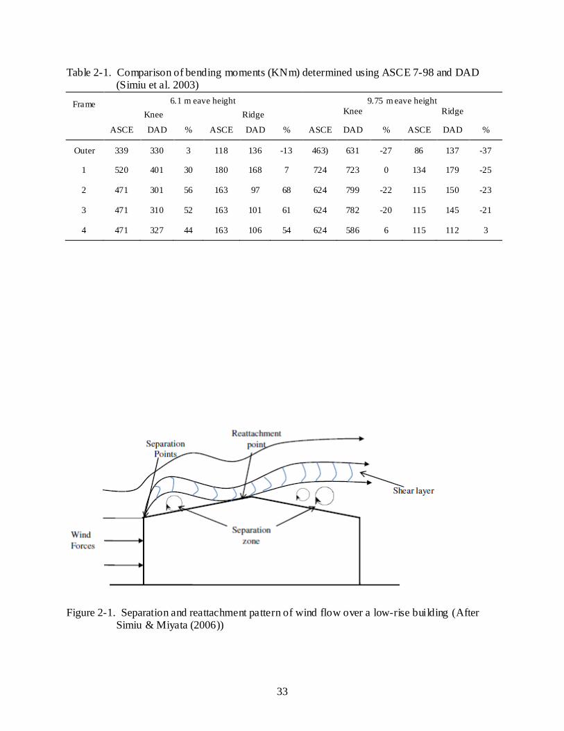
Wind flow over a low-rise building is characterized by separation and reattachment pattern

(shown in figure 2 -1) which together with its veloc ity fluc tuations generate a spatially and

temporally varying pressure field on the surface (Ginger et al. 2000). Ginger and Letchford

(1993) observed that large fluctuating suction pressures are generated in flow separation regions

close to the leading edges of the roof of low rise buildings. They explained that the flow

mechanisms that generate these pressures are the 2D separation bubble for flow perpendicular to

the edge discontinuity and the 3D conical vortex for flow at oblique angles to the edge

discontinuity and that the largest suction pressures are generated close to the leading corner for a

wind orientation of approximately 30°.

Ginger et al. (2000) determined wind loads on the roof of a typical low-rise house for

approach wind directions of 0o to 90o by carrying out a wind tunnel model study at a 1/50

geometric scale. They observed that the second truss from the windward gable end was subjected

to the largest wind load

Stathopoulos et al. (2000) conducted and presented a wind tunnel study which provided

detailed extreme local and area-averaged pressure coefficients for low-building roofs exposed to

open-country upstream terrains. They observed that when the wind flow is normal to the

ridgeline of a gable roof building, quasi- flat roofs in the range of 0o-30o create a similar flow

pattern of separation, entrainment, and reattachment; a high suction prevails, especially at the

20

windward edges and corners. They noted however that, if the roof angle is greater than 30o, wind

flow generally strikes on the windward roof prior to separating from the windward edge or ridge

which induces a positive pressure region on part of the windward slope and a negative region on

the leeward slope. They concluded that these flow patterns and pressure distributions may vary

with the wind direction, but remain comparable in respective roof slope ranges.

Current Design Provisions of ASCE 7 for Wind Loads on Low-Rise Buildings

Background on ASCE 7 Wind Load Provisions

The provisions of ASCE 7-05 for wind loads on low buildings are largely based on wind

tunnel study works conducted in the late 1970s at the boundary wind tunnel in the University of

Western Ontario (UWO)(Davenport et al. 1978; Stathopoulos 1979). Researchers at UWO used

an approach that consisted essentially of permitting the building model to rotate in the wind

tunnel through a full 360o in increments of 45o while simultaneously monitoring the loading

conditions on each surfaces. Both ope n and suburban expos ure conditions were considered.

Wind pressure coefficients which represent “pseudo” loading conditions, that when applied to a

building, envelope the desired structural actions (bending moment, shear, thrust), and the

maximum induced force components to be resisted for all possible directions and exposures were

developed from the studies (see C6.5.11 (ASCE/SEI. 2005)).

The current edition of the ASCE 7 standard (2005) has refined pressure and force

coefficients to reflect the latest boundary- layer wind tunnel and full-scale research findings. This

research has been however only limited to gable-roof buildings, and a rational method of

applying the coefficients to hip roofs based on experience, intuition and judgment has been

developed and presented in ASCE 7-05.

21

Three methods are provided in the ASCE 7 standard for determining wind design loads.

These are the “simplified method” (method 1), the analytical procedure (method 2) and a wind

tunnel procedure (method 3).

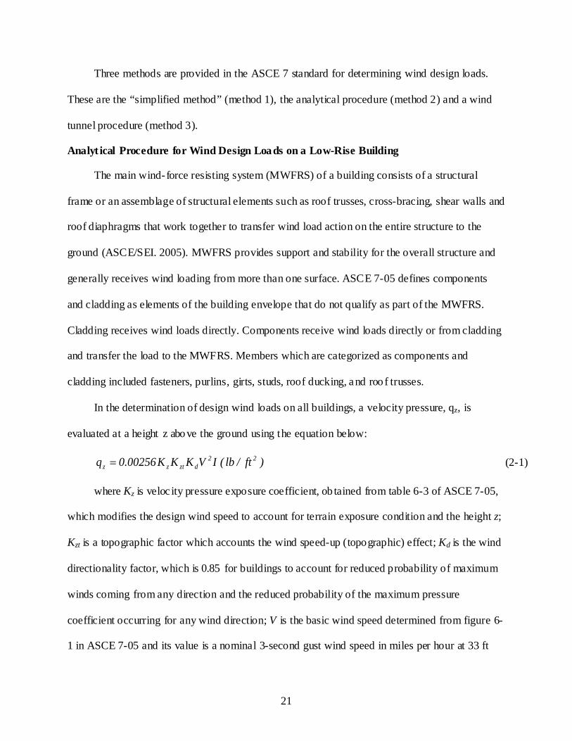
Analyt ical Procedure for Wind Design Loads on a Low-Rise Building

The main wind-force resisting system (MWFRS) of a building consists of a structural

frame or an assemblage of structural elements such as roof trusses, cross-bracing, shear walls and

roof diaphragms that work together to transfer wind load action on the entire structure to the

ground (ASCE/SEI. 2005). MWFRS provides support and stability for the overall structure and

generally receives wind loading from more than one surface. ASCE 7-05 defines components

and cladding as elements of the building envelope that do not qualify as part of the MWFRS.

Cladding receives wind loads directly. Components receive wind loads directly or from cladding

and transfer the load to the MWFRS. Members which are categorized as components and

cladding included fasteners, purlins, girts, studs, roof ducking, and roo f trusses.

In the determination of design wind loads on all buildings, a velocity pressure, qz, is

evaluated at a height z above the ground using the equation below:

)ft/lb(IVKKK00256.0q 22dztzz = (2-1)

where Kz is veloc ity pressure exposure coefficient, ob tained from table 6-3 of ASCE 7-05,

which modifies the design wind speed to account for terrain exposure condition and the height z;

Kzt is a topographic factor which accounts the wind speed-up (topographic) effect; Kd is the wind

directionality factor, which is 0.85 for buildings to account for reduced probability of maximum

winds coming from any direction and the reduced probability of the maximum pressure

coefficient occurring for any wind direction; V is the basic wind speed determined from figure 6-

1 in ASCE 7-05 and its value is a nominal 3-second gust wind speed in miles per hour at 33 ft

22

above ground for an open exposure; and I is importance factor of the building determined from

table 6-1 in ASCE 7-05 which is used to adjust the level of reliability of building or structure to

be consistent with the building c lassifications indicated in the standard.

Design wind pressures, for both MWFRS and components and cladding, are determined as

the product of the veloc ity pressure and the sum of internal and external pressure coefficients.

The internal pressure coefficients, GCpi are provided in figure 6-5 o f ASCE 7-05 in terms of the

building enclosure classification (i.e. open, partially enclosed or enclosed building). The external

pressure coefficients are given separately for MWFRS and components and cladding for

different scenarios but generally in terms of pressure zones. Pressure zones specified in the

ASCE standard for both MWRS and Components and Cladding are in terms of a dimension

denoted by a (Simiu and Miyata 2006). The dimension a is 10% of the least horizontal building

dimension or 0.4 h (h=mean roo f height), whichever is smaller, but not less than 4% of the least

horizontal building dimension or 3ft.

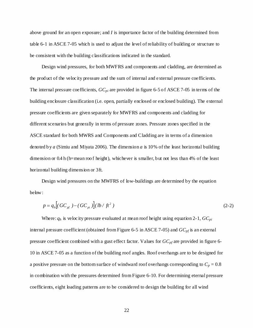
Design wind pressures on the MWFRS of low-buildings are determined by the equation

below:

[ ] )ft/lb()GC()GC(qp 2pipfh −= (2-2)

Where: qh is veloc ity pressure evaluated at mean roof height using equation 2-1, GCpi

internal pressure coefficient (obtained from Figure 6-5 in ASCE 7-05) and GCpf is an external

pressure coefficient combined with a gust effect factor. Values for GCpf are provided in figure 6-

10 in ASCE 7-05 as a function of the building roof angles. Roof overhangs are to be designed for

a positive pressure on the bottom surface of windward roof overhangs corresponding to Cp = 0.8

in combination with the pressures determined from Figure 6-10. For determining eternal pressure

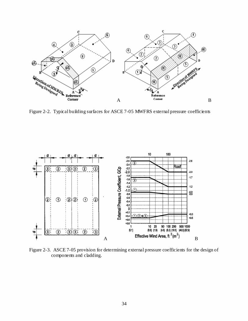
coefficients, eight loading patterns are to be considered to design the building for all wind

23

directions. The loading patterns have the walls and roofs zoned into several building surfaces

which envelope wind load distributions on the building. Figure 2-2 shows typical load patterns

in the ASCE 7-05 for wind design loads on a MWFRS of a building.

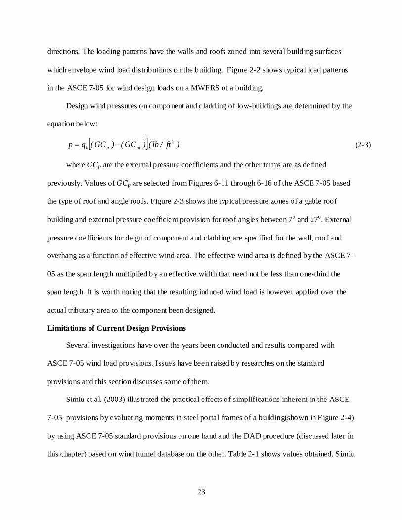
Design wind p ressures on component and c ladd ing of low-buildings are determined by the

equation below:

[ ] )ft/lb()GC()GC(qp 2piph −= (2-3)

where GCp are the external pressure coefficients and the other terms are as defined

previously. Values of GCp are selected from Figures 6-11 through 6-16 of the ASCE 7-05 based

the type of roof and angle roofs. Figure 2-3 shows the typical pressure zones of a gable roof

building and external pressure coefficient provision for roof angles between 7o and 27o. External

pressure coefficients for deign of component and cladding are specified for the wall, roof and

overhang as a function of effective wind area. The effective wind area is defined by the ASCE 7-

05 as the span length multiplied by an effective width that need not be less than one-third the

span length. It is worth noting that the resulting induced wind load is however applied over the

actual tributary area to the component been designed.

Limitations of Current Design Provisions

Several investigations have over the years been conducted and results compared with

ASCE 7-05 wind load provisions. Issues have been raised by researches on the standard

provisions and this section discusses some of them.

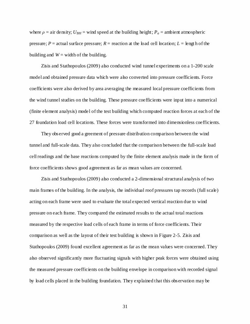
Simiu et al. (2003) illustrated the practical effects of simplifications inherent in the ASCE

7-05 provisions by evaluating moments in steel portal frames of a building(shown in F igure 2-4)

by using ASCE 7-05 standard provisions on one hand and the DAD procedure (discussed later in

this chapter) based on wind tunnel database on the other. Table 2-1 shows values obtained. Simiu

24

et al. (2003) demonstrated that the use of the tables and plots in wind load design provisions can

entail errors that can exceed 50% in the estimation of wind effects.

Furthermore, Whalen et al. (2002) assert that the accuracy in the definition of wind loads

inherent in such tables and plots are lower than that inherent in current methods for stress

computation. There is so much complexity with geometries and shapes of low-rise buildings and

hence high accuracy in predicting design loads based on tables and plots cannot be achieved.

Wind directionality effects on low-rise buildings are accounted for in the ASCE 7 standard

by a reduction factor of 0.85. Simiu et al. (2003) observed that this approach is inadequate as

wind effect reductions due to directionality effects are less significant as the mean recurrence

interval of the wind effects increase, rending the use of this factor potentially unsafe, particularly

for MWFRS.

Design parameters such as building geometry, building orientation, proximity of adjacent

structures and, the spatial and temporal variation of wind loads are not realistically and

comprehensively accounted for when a designer uses the conventional standard provisions

(Simiu and Stathopoulos 1997).

Recently, wind tunnel test data on generic low buildings were obtained at UWO to

contribute to the National Institute of Standards and Technology (NIST) aerodynamic database

(Ho et al. 2005b). St. Pierre et al. (2005) compared the NIST aerodynamic database to the

historical data obtained by Stathopoulos in the late 1970s, from which the current ASCE 7

provisions were developed. They observed that for the exterior bay of the test building model,

ASCE 7 generally underestimates the response coefficients significantly. For the interior bays,

the ASCE 7 overestimates the response coefficients. They also observed that generally, there was

10-85% underestimation of peak response coefficients in the suburban terrain by ASCE 7.

25

Attempts by writers of the standard provisions on wind loads to reduce the limitations of

earlier versions of the standard (example ASCE 7-05) resulted in bulky and complex provisions

(Simiu and Stathopoulos 1997).

Database-Assisted Design (DAD) Methodology for a Low-Rise Building

Background of the DAD methodology

With the backdrop of the above mentioned limitations of the wind design load provisions,

it was necessary to work on an alternative approach which offers the potential for significantly

more risk-consistent, realistic, safer and economical design by using adequate aerodynamic

databases and information. Owning to current information storage and computational

capabilities, Simiu and Stathopoulos (1997) proposed a new generation of standard with

provisions on wind loads that are no longer based on reductive and distorting tables and plots,

but can be structured on knowledge-based systems drawing the requisite information from large

databases.

Their postulation was that, wind loads evaluated via the new methodology would be

functions of design parameters, which includes building geometry, building orientation, position

with respect to and geometry of neighboring buildings, built-up terrain roughness, etc. They

intimated that their proposal would allow the designer to target specific situations, rather than

providing blanket coverage for a broad range of situations. They explained that this methodology

would furthermore allow the designer to account for the specific linear or nonlinear structural

characteristics of the building or structure (eg. influence function).

Subsequently, Whalen et al. (1998) conducted a pilot project on the estimation of wind

effects in low-rise building frames using this methodology. Whalen et al. (1998) used records of

pressure time histories measured at large number of taps on a building surface at the UWO

boundary layer wind tunnel. Time histories of bending moments in a frame were obtained by

26

summing up pressures time histories tributary to that frame multiplied by the respective tributary

areas and frame influence coefficients. They compared results with results based on ASCE 7

standard provisions. Their comparison suggested that, significantly more risk-consistent, safer

and economical designs could be achieved using this approach than using conventional standard

provisions.

The approach of using electronic aerodynamic and climatological databases to define wind

loads was coined “database-assisted design” (DAD) and was accepted by the ASCE 7-98

standard (Rigato et al. 2001) .

DAD Concept and Software Development

The first generation DAD application called WiLDE-LRS – Wind Load Design

Environment for Low-rise Structures was developed by NIST (Whalen et al. 2000). WiLDE-

LRS, a MATLAB®-based software, adopted interactive graphical user interfaces (GUI) to give a

visual, user- friendly design environment. MATLAB scripts were used in the software to analyze

the behavior of rigid portal frames and other components under high winds and to produce time

histories of wind load effects in these structural members. The software had its origins in a

prototype application called Frameloads, used to study wind effects on moment resisting frames

in low-rise buildings designed by the Standard Metal Building Manufactures Association

methodology. A latter version (2.7 ) of WiLDE-LRS (Whalen et al. 2002) greatly enhanced the

GUIs that directly accepted input of influence coefficients accounting for frame properties. Post-

processing was incorporated in this version to calculate realistic and robust statistical estimates

of the peak load effect values based upon the entire time history.

Subsequently, the DAD approach has been extended to consider nonlinear static response

of low buildings (Jang et al. 2002) and also to account for the probability distribution of the

peaks of time histories of wind e ffects and of sampling errors in the estimation of that

27

distribution (Sadek and Simiu 2002; Sadek et al. 2004). A scheme to interpolate existing data in

available database to other configurations in a reliable, accurate and simple way, without

resorting to further wind tunnel experiments, has been incorporated in DAD applications (Kopp

and Chen 2006).

In 2006, NIST released software packages developed using the MATLAB language to

fully implement the DAD approach and all its improvements (Main and Fritz 2006). Two

separate software packages are available through the internet at http://www.nist.gov/wind for

rigid, gable-roofed buildings and for tall, flexible buildings.

Limitation to the Application of DAD Approach

To the best of author’s knowledge:

1. Application of the DAD approach and its software has been limited to steel portal frame buildings.

2. Structural influence functions used by researches so far in DAD applications have been analytically derived using hand-calculations or 2-D models in structural analysis software

3. .The validity of the approach has not been demonstrated experimentally.

Design and Construction of Light Framed Wood Structures and their Performance to Wind Forces

Wood-frame construction forms the major ity of residential and other low-rise structures. A

number of these structures are located along hurricane-prone zones in the United States. This

section discusses the construction methods prevalent in the wood -frame industry and their

performance during hurricane events. The literature presented here is based on studies done by

Rosowsky and Schiff (2003) and van de Lindt et al. (2007).

Construction Methods

Three construction methods have been identified by van de Lindt et al. (2007). These are

the conventional, engineered and prescriptive. The conventional method consists of following

http://www.nist.gov/wind�

28

documents such as the International Residential Code outlining certain exceptions and

limitations. Most wood constructions are based on conventional methods. For engineered

construction, structures are specifically designed by a design professional to meet jurisdictional

requirements. Interestingly, very few residential buildings are engineered. Prescriptive

construction invo lves the use of basic material strength level and tabulated values obtained from

construction manuals.

Rosowsky and Schiff (2003) referred to designs based on the conventional method as

deemed-to-comply design, which is largely derived from traditional rules of thumb for building

light- frame wood structures (LFWS). They observed that most of the rules focused on building

structures to safely resist gravity loads, ignoring geographic considerations. Until recently, most

buildings, including those located in high-wind environments, were constructed using

conventional methods which did not meet wind-resistant design requirements. This caused these

structures to have the greatest vulnerability to extreme wind events.

Critical Components and Systems

According to Rosowsky and Schiff (2003), the three most important areas to consider in

designing a wind-resistant wood-frame structure are:

1. The building envelope : This forms the first line of defense against wind and water intrusion. Traditionally, the building envelope is considered to be architecture in nature and therefore not designed by engineers. However, s tudies have shown that a direct correlation exists between the performance and damage (losses) sustained by wood-frame buildings. Structural engineers are becoming actively involved in the building envelope designs.

2. Attachment of roof and wall sheathing: this component is critical in keeping structures enclosed, preventing infiltration and providing critical links in the structural load path. Removal of roof sheathing is the second largest failure mode observed in post-hurricane investigation after removal of roof cover. Significant highlight has been given to the need to provide more and larger fasteners around roof edges to resist high wind uplift pressures.

29

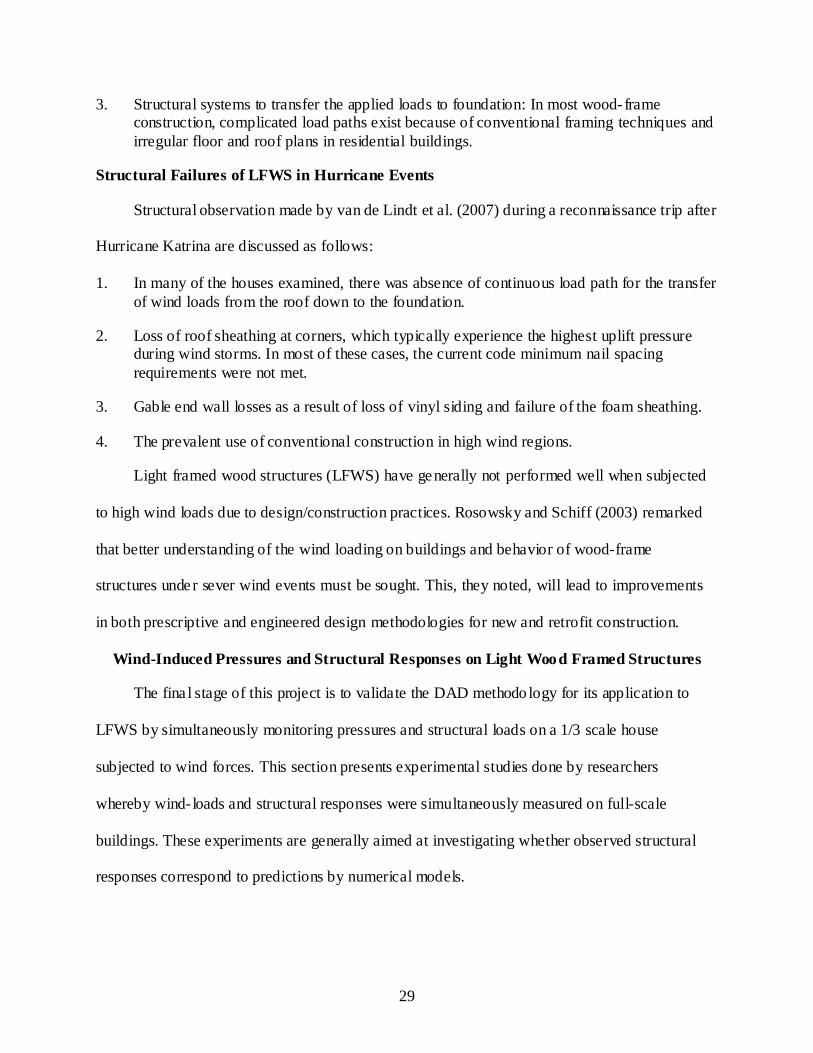
3. Structural systems to transfer the applied loads to foundation: In most wood- frame construction, complicated load paths exist because of conventional framing techniques and irregular floor and roof plans in residential buildings.

Structural Failures of LFWS in Hurricane Events

Structural observation made by van de Lindt et al. (2007) during a reconnaissance trip after

Hurricane Katrina are discussed as follows:

1. In many of the houses examined, there was absence of continuous load path for the transfer of wind loads from the roof down to the foundation.

2. Loss of roof sheathing at corners, which typically experience the highest uplift pressure during wind storms. In most of these cases, the current code minimum nail spacing requirements were not met.

3. Gable end wall losses as a result of loss of vinyl siding and failure of the foam sheathing.

4. The prevalent use of conventional construction in high wind regions.

Light framed wood structures (LFWS) have generally not performed well when subjected

to high wind loads due to design/construction practices. Rosowsky and Schiff (2003) remarked

that better understanding of the wind loading on buildings and behavior of wood-frame

structures under sever wind events must be sought. This, they noted, will lead to improvements

in both prescriptive and engineered design methodologies for new and retrofit construction.

Wind-Induced Pressures and Structural Responses on Light Wood Framed Structures

The fina l stage of this project is to validate the DAD methodo logy for its application to

LFWS by simultaneously monitoring pressures and structural loads on a 1/3 scale house

subjected to wind forces. This section presents experimental studies done by researchers

whereby wind- loads and structural responses were simultaneously measured on full-scale

buildings. These experiments are generally aimed at investigating whether observed structural

responses correspond to predictions by numerical models.

30

Doudak et al. (2005) monitored a single story industrial shed building to de termine its

displacement response to wind and snow loads. He attempted to correlate the observed

displacements with real-time estimates using SAP 2000 of these environmental loads. Wind

speed and direction was measured as well as displacements on the building during the typical

wind storm season. Doudak et al. (2005) however did not take pressure measurements on the

house. Wind pressures for numerical simulations were estimated from archived pressure

coefficients and the measured wind speeds. They achieved a quite reasonable agreement between

measured and predicted displacements. Discrepancies ranged from as low as 6 % in most cases

to as high as 90 % for all four incident wind d irections.

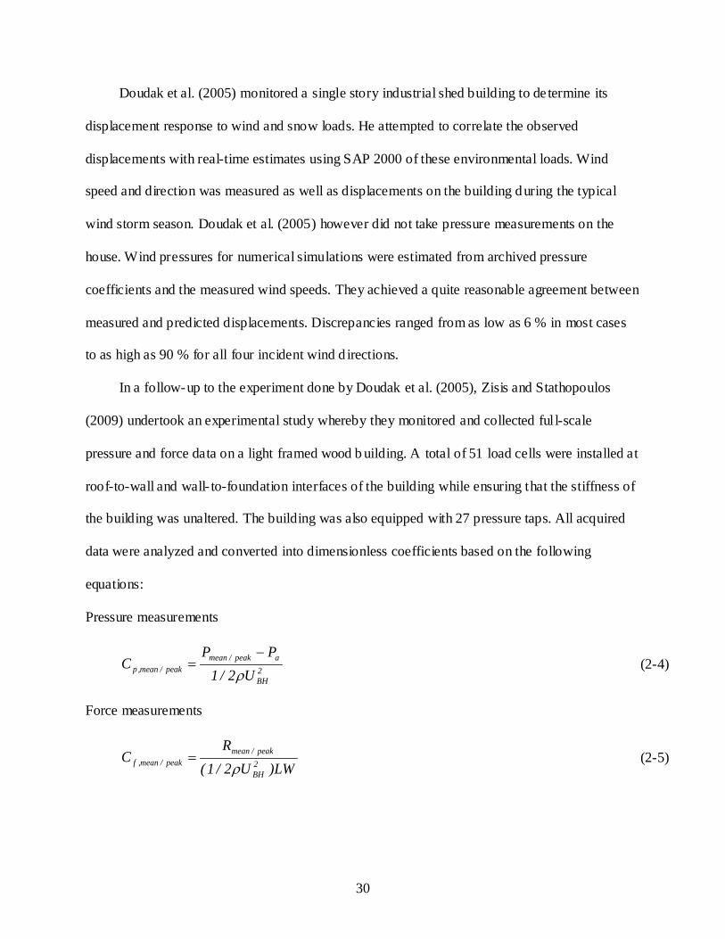
In a follow-up to the experiment done by Doudak et al. (2005), Zisis and Stathopoulos

(2009) undertook an experimental study whereby they monitored and collected ful l-scale

pressure and force data on a light framed wood b uilding. A total of 51 load cells were installed at

roof-to-wall and wall- to-foundation interfaces of the building while ensuring that the stiffness of

the building was unaltered. The building was also equipped with 27 pressure taps. All acquired

data were analyzed and converted into dimensionless coefficients based on the following

equations:

Pressure measurements

2BH

apeak/meanpeak/mean,p U2/1

PPC

ρ−

= (2-4)

Force measurements

LW)U2/1(R

C 2BH

peak/meanpeak/mean,f ρ

= (2-5)

31

where ρ = air density; UBH = wind speed at the building height; Pa = ambient atmospheric

pressure; P = actual surface pressure; R = reaction at the load cell location; L = lengt h of the

building and W = width of the building.

Zisis and Stathopoulos (2009) also conducted wind tunnel experiments on a 1-200 scale

model and obtained pressure data which were also converted into pressure coefficients. Force

coefficients were also derived by area averaging the measured local pressure coefficients from

the wind tunnel studies on the building. These pressure coefficients were input into a numerical

(finite element analysis) model of the test building which computed reaction forces at each of the

27 foundation load cell locations. These forces were transformed into dimensionless coefficients.

They observed good a greement of pressure distribution comparison between the wind

tunnel and full-scale data. They also concluded that the comparison between the full-scale load

cell readings and the base reactions computed by the finite element analysis made in the form of

force coefficients shows good agreement as far as mean values are concerned.

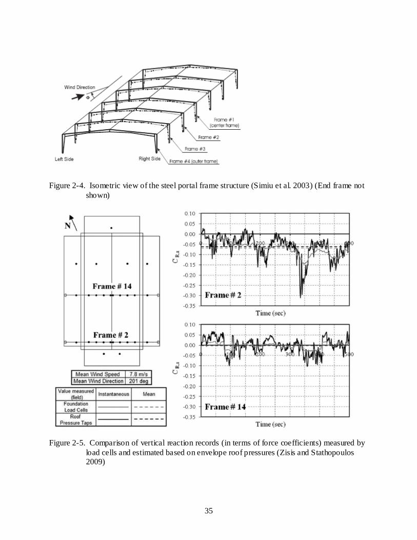
Zisis and Stathopoulos (2009) also conducted a 2-dimensional structural analysis of two

main frames of the building. In the analysis, the individual roof pressures tap records (full scale)

acting on each frame were used to evaluate the total expected vertical reaction due to wind

pressure on each frame. They compared the estimated results to the actual total reactions

measured by the respective load cells of each frame in terms of force coefficients. Their

comparison as well as the layout of their test building is shown in Figure 2-5. Zisis and

Stathopoulos (2009) found excellent agreement as far as the mean values were concerned. They

also observed significantly more fluctuating signals with higher peak forces were obtained using

the measured pressure coefficients on the building envelope in comparison with recorded signal

by load cells placed in the building foundation. They explained that this observation may be

32

partly attributed to the dynamic load attenuation effect due to structural and material damping of

the building components hence lower reactions measured than computed.

Both experimental studies discussed above exposed the test buildings to natural wind

forces. Consequently, wind pressure data collected from the field was highly affected by

fluctuations of wind directions during the test. Moreover, the structure does not experience winds

that would cause the worst load effects or design level events.

33

Table 2-1. Comparison of bending moments (KNm) determined using ASCE 7-98 and DAD (Simiu et al. 2003)

Frame

6.1 m eave height 9.75 m eave height Knee Ridge Knee Ridge

ASCE DAD % ASCE DAD % ASCE DAD % ASCE DAD %

Outer 339 330 3 118 136 -13 463) 631 -27 86 137 -37

1 520 401 30 180 168 7 724 723 0 134 179 -25

2 471 301 56 163 97 68 624 799 -22 115 150 -23

3 471 310 52 163 101 61 624 782 -20 115 145 -21

4 471 327 44 163 106 54 624 586 6 115 112 3

Figure 2-1. Separation and reattachment pattern of wind flow over a low-rise building (After

Simiu & Miyata (2006))

34

A B Figure 2-2. Typical building surfaces for ASCE 7-05 MWFRS external pressure coefficients

A B Figure 2-3. ASCE 7-05 provision for determining external pressure coefficients for the design of

components and cladding.

35

Figure 2-4. Isometric view of the steel portal frame structure (Simiu et al. 2003) (End frame not

shown)

Figure 2-5. Comparison of vertical reaction records (in terms of force coefficients) measured by

load cells and estimated based on envelope roof pressures (Zisis and Stathopoulos 2009)

36

CHAPTER 3 ANAYSIS OF WIND TUNNEL DATA TO GENERATE PRESSURE COEFFICIENTS

Wind Tunnel Data

For this study, pressure coefficients were derived from wind tunnel data developed by

Datin and Prevatt (2007) on a 1:50 scale model house. The experiments were carried out in an

atmospheric boundary layer wind tunnel at the Wind Load Test Facility (WLTF) at Clemson

University. An overview of the experiment is discussed below.

House Model and Pressure Tap Layo ut

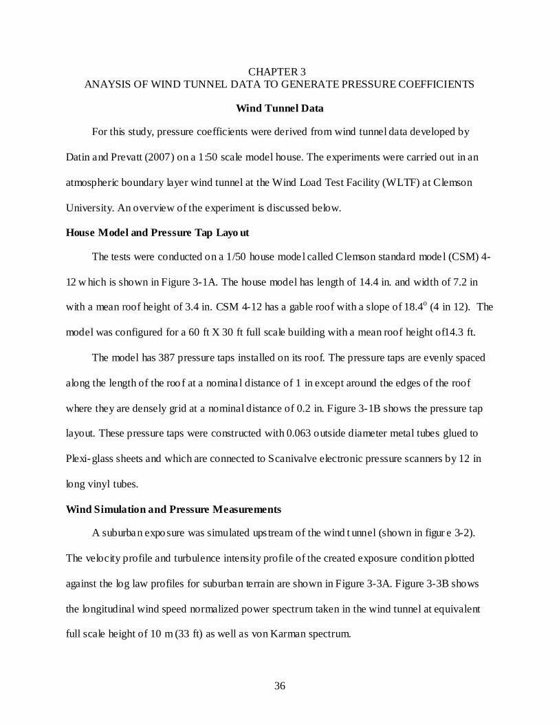
The tests were conducted on a 1/50 house model called Clemson standard model (CSM) 4-

12 w hich is shown in Figure 3-1A. The house model has length of 14.4 in. and width of 7.2 in

with a mean roof height of 3.4 in. CSM 4-12 has a gable roof with a slope of 18.4o (4 in 12). The

model was configured for a 60 ft X 30 ft full scale building with a mean roof height of14.3 ft.

The model has 387 pressure taps installed on its roof. The pressure taps are evenly spaced

along the length of the roo f at a nomina l distance of 1 in except around the edges of the roof

where they are densely grid at a nominal distance of 0.2 in. Figure 3-1B shows the pressure tap

layout. These pressure taps were constructed with 0.063 outside diameter metal tubes glued to

Plexi-glass sheets and which are connected to Scanivalve electronic pressure scanners by 12 in

long vinyl tubes.

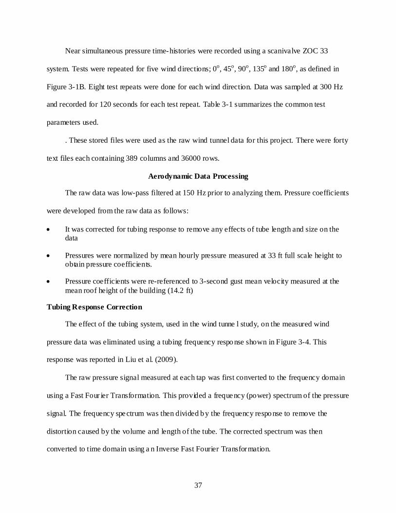
Wind Simulation and Pressure Measurements

A suburban exposure was simulated ups tream of the wind t unnel (shown in figur e 3-2).

The velocity profile and turbulence intensity profile of the created exposure condition plotted

against the log law profiles for suburban terrain are shown in Figure 3-3A. Figure 3-3B shows

the longitudinal wind speed normalized power spectrum taken in the wind tunnel at equivalent

full scale height of 10 m (33 ft) as well as von Karman spectrum.

37

Near simultaneous pressure time-histories were recorded using a scanivalve ZOC 33

system. Tests were repeated for five wind directions; 0o, 45o, 90o, 135o and 180o, as defined in

Figure 3-1B. Eight test repeats were done for each wind direction. Data was sampled at 300 Hz

and recorded for 120 seconds for each test repeat. Table 3-1 summarizes the common test

parameters used.

. These stored files were used as the raw wind tunnel data for this project. There were forty

text files each containing 389 columns and 36000 rows.

Aerodynamic Data Processing

The raw data was low-pass filtered at 150 Hz prior to analyzing them. Pressure coefficients

were developed from the raw data as follows:

• It was corrected for tubing response to remove any effects of tube length and size on the data

• Pressures were normalized by mean hourly pressure measured at 33 ft full scale height to obtain pressure coefficients.

• Pressure coefficients were re-referenced to 3-second gust mean velocity measured at the mean roof height of the building (14.2 ft)

Tubing Response Correction

The effect of the tubing system, used in the wind tunne l study, on the measured wind

pressure data was eliminated using a tubing frequency response shown in Figure 3-4. This

response was reported in Liu et al. (2009).

The raw pressure signal measured at each tap was first converted to the frequency domain

using a Fast Four ier Transformation. This provided a frequency (power) spectrum of the pressure

signal. The frequency spectrum was then divided by the frequency response to remove the

distortion caused by the volume and length of the tube. The corrected spectrum was then

converted to time domain using a n Inverse Fast Fourier Transformation.

38

Determining Pressure Coefficients

Pressure coefficients were derived from the measured local pressure time series as follows:

)(P),t(P

),t(Cref

ii,ref,p θ

θθ =

(3-1)

where, Cp,ref,i(t,θ) is the pressure coefficient at Pressure Tap i, referenced to the dynamic pressure

at reference height, at time t for wind angle θ; Pi(t,θ) is the measured wind pressure at tap i at

time t for wind angle θ; )(Pref θ is the mean hour ly reference dynamic pressure recorded by a

Pitot tube at the reference height of full height of 33ft for wind angle θ. Pressure coefficients

were referenced at that height because flow is uniform with low turbulence levels at that height.

This ensures accurate speed control of the wind tunnel and accurate calibration of the pressure

scanners (Ho et al. 2005a).

Re-referencing of Pressure Coefficients

It is widely accepted that aerodynamic data referenced to mean roof height dynamic

pressure produce the least variability and therefore all low building pressure data sets, including

those in the building codes, follow this convention (Ho et al. 2005a). I t is intended that the wind

tunnel results should be comparable to those in ASCE 7 and other aerodynamic database. For

this reason, the wind pressure coefficients were normalized to a 3-second gust mean wind speed

at the mean roof height (14.3 ft full-scale), mrhsec,3U . The wind pressure coefficients Cp,ref,i(t,θ)

were converted to the equivalent coefficient as follows.

),(),( ,,, θθ tCCtC irefpaip ×= (3-2)

where, Cp,i(t,θ) is the wind pressure coefficients at pressure tap i, referenced to a 3-second gust

wind speed at the mean roof height, at time t for wind angle θ; and Ca is an adjustment factor

39

which is given by the squared ratio o f the mean wind speed a t reference height refU to the

equivalent 3-second gust wind speed at mean roof height mrhsec,3U (Shown in Equation 3-3).

2mrhsec,3

2ref

aU

UC =

(3-3)

The mean hourly wind speeds at the reference height refU (13.03 m/s) and mean roo f

height Umrh (6.54 m/s) were determined from the velocity profile for the wind tunnel testing. The

ASCE 7-05 provides the Durst curve which relates the wind speed averaged over gust duration, t

(in seconds), Ut to hourly mean speed, U3600. However, the curved corresponds to open terrain

conditions and an elevation, z = 10 m (Simiu and Scanlan 1996). As already stated, the wind

tunnel data was developed for a suburban terrain condition and pressure coefficients are intended

to be referenced to mean roof height of 14.3 ft (4.2 m). Hence, conversion of the mean hourly

speed to 3-second gust was done us ing Equation 3-4 provided by Simiu & Scanlan (1996).

+=

o

3600t

zzln5.2

)t(C1)z(U)z(Uβ

(3-4)

where, C(t) is the time averaging constant for a given time averaging interval β is the squared

ratio of the friction veloc ity to the longitudina l turbulence fluctuations; zo is the roughness length;

z is the height at which the wind speed is to be evaluated. The calculation of 3-second gust wind

speed at mean roof height, which was based on C(3sec) =2.85; zo = 0.22m, z = 4.2m (14.3ft) and

β = 5.25, is as follows:

+=

o

mrhmrhsec,3

zzln5.2

sec)3(C1UUβ

(3-5)

40

s/m33.12

m22.0m2.4ln5.2

25.585.21)s/m54.6(U mrhsec,3 =

+=

(3-6)

The resulting adjustment factor, Ca for re-referencing the pressure coefficients is 1.1168.

Wind Tunnel Results and Analysis

Wind Pressure Coefficients Time Histories

The resulting pressure coefficient time histories were converted to equivalent full-scale

pressure coefficients using the reduced frequency relationship shown in Equation 3-7.

pm VfL

VfL

=

(3-7)

where f, L and V are respectively sampling frequency, characteristic dimension, and wind speed

referenced at mean height over a specified duration. Subscripts m and p denote model (1:50

scale) and prototype (full scale) buildings respectively. Based on mode l frequency and 3-second

gust wind speed at mean roof height of 300 Hz and 29 mph respectively, and 3-second gust full

scale wind speed, at mean roof height of prototype for suburban terrain, of 80.27 mph, the

prototype frequency is calculated as:

mph27.8050f

mph291Hz300 p ×=

× Hz46.17f p =

(3-8)

Using equality of non-dimensional time, the equivalent ful l-scale duration is given by:

m

mpp f

TfT

×=

(3-9)

Hz46.17s120Hz300Tp

×=

utesmin36.34Tp =

(3-10)

The equivalent full-scale time step for the time histories is:

41

s0573.0Hz46.17

1f1t

pp === (3-11)

Pressure coefficient time histories in duration of 34 minutes in full scale of the 387

pressure taps were generated for each sample of a wind direction. Calculation for determining

the equivalent full-scale duration of the 120 seconds of test period is presented in the appendix.

Figure 3-5 shows time series plots pressure coefficients at pressure taps 1 and 387 for wind

direction 0o.

Pressure coefficient time series, which are useful for analyzing dynamic responses of low-

rise buildings; have been saved in a MATLAB da ta format, as shown in Figure 3-3. There are 40

binary files with filenames structured as “CSM4-12_Suburban_Cp_data_dir_XXX_Y.mat”,

where “CSM4-12” identifies that the “Clemson Standard Model” with a roof slope of 4-12 was

used in the wind tunnel study; “XXX” denotes the wind direction; and “Y” denotes the sample

number. Each file also contains information of full scale geometric properties of the building

model tested, sampling frequency and period, time-step, locations of the pressure taps on model,

data sample number, wind azimuth, etc.

Observed Statistical Values of Wind Pressure Coefficients

The sample mean, root mean square (RMS) and peak local pressure coefficients were

computed for the eight samples of each wind azimuth. The statistical values of pressure

coefficients, which are useful for the design of cladding and components such as roof fasteners,

purlins and panes, have been evaluated for 34-minute equivalent full-scale aerodynamic pressure

coefficient time histories. These values were also saved in the for ty MATLAB files containing

the pressure coefficient time histories. The mean and RMS pressure coefficient values were

averaged values of the eight samples:

42

∑=

=8

1ni,pi,p ),n(C

81)(C θθ

(3-12)

∑=

=8

1ni,pi,p ),n(C

81)(C θθ (3-13)

where, )(C i,p θ and )(C i,p θ are respectively the mean and RMS pressure coefficients for at

pressure tap i, for wind angle θ of the entire experiment; and ),n(C i,p θ and ),n(C i,p θ are

respectively the mean and RMS values of time series of the nth sample i, for wind angle θ.

Contour plots of mean and RMS pressure coefficients measured for each direction are shown in

Figures 3-7 and 3-8.

Extreme Value Analysis of Pressure Coefficients

Peak values estimated based on a probability distribution function are generally more

statistically stable quantities than the observed peaks from individual samples (Ho et al. 2005a).

The extreme negative and positive pressure coefficients measured from the eight samples of each

wind direction were fitted to an Extreme Type 1 Value Distribution. The probability density

function (PDF) and the cumulative distribut ive func tion (CDF) of the Extreme value Type 1

(also referred to as Gumbel distribution) are given by:

βµβµ

β)x()x( ee1)x(f −−−= (3-14)

βµ )x(e)x(F −−= (3-15)

where, µ is the location parameter (mode); and β is the scale parameter (NIST 2003). The

parameters were calculated using the Best Linear Unbiased Estimators (BLUE) (Lieblein 1974).

There are three methods proposed by Lieblein (1974) based on sample sizes for the estimation of

the location and scale parameters. Method o ne is for an analys is with sample size less than

43

sixteen. The second method s hould be used for a study with sample size larger than sixteen but

generally smaller than about fifty. For an analysis with larger same size, method three is to be

used. The first method is adopted in this study since the sample size is eight. Furthermore, for

this analysis, the peak negative pressure coefficients were multiplied by negative one to make

them positive since BLUE analysis was developed for maximum values of the Type I extreme

Value distribution. The pos itive values were then sorted in the ascending order to p lace them in

the following order:

821 x...xx ≤≤≤

The loc ation parameter, µ and the scale parameter, β were then estimated as follows:

∑=

=8

1nii xaµ ∑

=

=8

1nii xbβ

(3-16)

where, xi is the ith value of the ascending array of maximum values of the eight samples and ai

and bi are given by Table 3-2.

The “best” expected (mean) peak pressure coefficient measured at each pressure tap in a

given wind direction is given by:

βµ 5772.0+=∧

pC (3-17)

Figures 3-9 and 3-10 show the spatial variations of the expected extreme pressure

coe fficients on the roo f of the building for different wind d irections. The roo f corners and gable

edges experience spatial variations at close distances and higher magnitude of suctions for all

wind directions except for wind direction 90o. A nearly even distribution is observed away from

roof edges and corners. A similar pattern is observed be tween the mean, RMS and extreme

pressure coefficient distributions of wind azimuths 45o and 135o are at opposing angles. The

same observation is made between the distributions of 0o and 180o. Appendix A provides mean,

44

RMS and extreme pressure coefficients of selected pressure taps for wind azimuths 0o, 45oand

90o.

Area-Averaged Pressure Coefficients

Area-averaged pressure coefficients have been derived from pressure coefficient time

histories for regions of different size as follows:

∑ ∑= =

×=j jN

i

N

iiipF AAitCtjC

1 1/)),((),(

(3-18)

where CF(t) is a area-averaged wind pressure coefficient on region j at time t; Cp(i,t) is the wind

pressure coefficient at pressure tap i at time t; Ai is the tributary area of pressure tap i and Nj is

the total number of pressure taps on region j.

The mean, RMS and extreme values of area-averaged pressure coefficients for the eight

samples of each direction were determined. The average mean and RMS of were calculated as

discussed above, while an extreme value analysis was done to determine the peak negative and

positive area-averaged pressure coefficients. Figures 3-11 to 3-13 display the area-averaged

pressure coefficients as a function of wind azimuth for corner, ridge corner, eave, ridge, interior,

and gable edge, corner, ridge corner, eave, ridge, interior, and gable edge. These pressure

coefficient values measured in the different regions on the surface of the building are compared

to ASCE 7-05 external wind pressure coefficients for components and cladding provided in

Figure 6-11C of the ASCE 7-05. Table 3-3 provides a summary of peak local pressure

coefficients observed within each of the three zones defined in ASCE 7-05, the area averaged

pressure coefficients and the C&C external pressure coefficients corresponding to the zones.

It is observed that, the peak local (tap) negative pressures (suctions) are generally higher in

magnitude as compared to the ASCE 7-05 provisions for the design of components and c ladding.

45

However, the peak area-averaged pressure coefficients measured for each zone fall within the

provisions of ASCE 7 for the various zones. Also, it is observed that, the peak area averaged

pressure coefficients for two wind directions (i.e. 0o and 180o; and 45o and 135o) are ide nt ical.

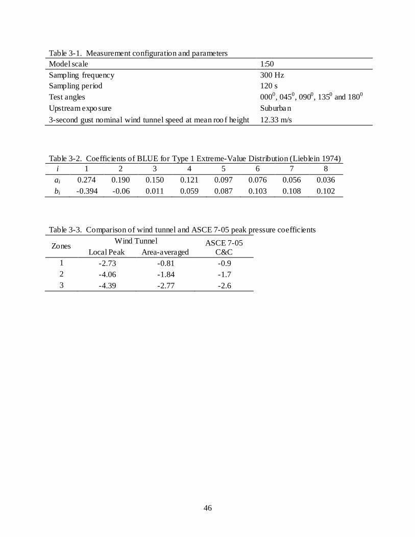
46

Table 3-1. Measurement configuration and parameters Model scale 1:50 Sampling frequency 300 Hz Sampling period 120 s Test angles 0000, 0450, 0900, 1350 and 1800 Upstream exposure Suburban 3-second gust nominal wind tunnel speed at mean roo f height 12.33 m/s Table 3-2. Coefficients of BLUE for Type 1 Extreme-Value Distribution (Lieblein 1974)

i 1 2 3 4 5 6 7 8 ai 0.274 0.190 0.150 0.121 0.097 0.076 0.056 0.036 bi -0.394 -0.06 0.011 0.059 0.087 0.103 0.108 0.102

Table 3-3. Comparison of wind tunnel and ASCE 7-05 peak pressure coefficients

Zones Wind Tunnel ASCE 7-05 C&C Local Peak Area-averaged

1 -2.73 -0.81 -0.9 2 -4.06 -1.84 -1.7 3 -4.39 -2.77 -2.6

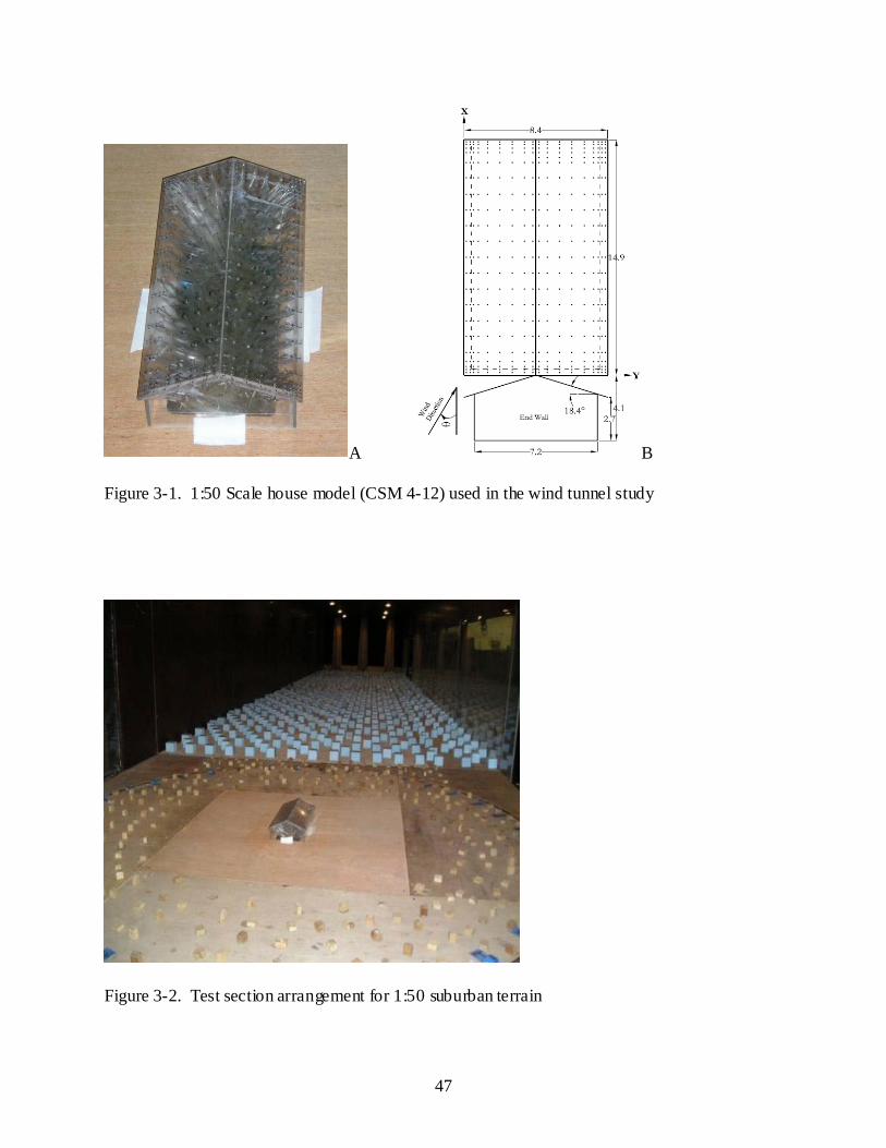
47

A B Figure 3-1. 1:50 Scale house model (CSM 4-12) used in the wind tunnel study

Figure 3-2. Test section arrangement for 1:50 suburban terrain

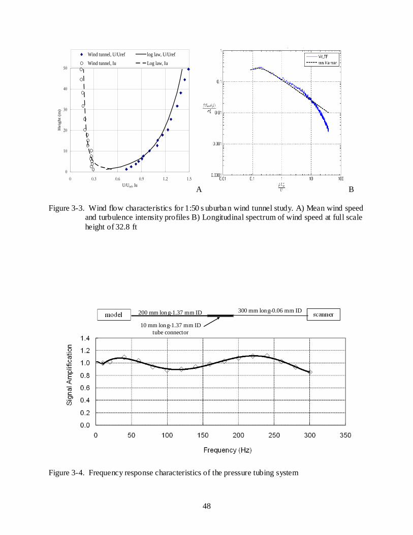
48

0

10

20

30

40

50

0 0.3 0.6 0.9 1.2 1.5U/Uref, Iu

Hei

ght (

m)

Wind tunnel, U/Uref log law, U/UrefWind tunnel, Iu Log law, Iu

A B Figure 3-3. Wind flow characteristics for 1:50 s uburban wind tunnel study. A) Mean wind speed

and turbulence intensity profiles B) Longitudinal spectrum of wind speed at full scale height of 32.8 ft

Figure 3-4. Frequency response characteristics of the pressure tubing system

200 mm long-1.37 mm ID 300 mm long-0.06 mm ID

10 mm long-1.37 mm ID tube connector

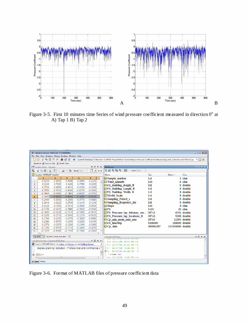
49

A B Figure 3-5. First 10 minutes time Series of wind pressure coefficient measured in direction 0o at

A) Tap 1 B) Tap 2

Figure 3-6. Format of MATLAB files of pressure coefficient data

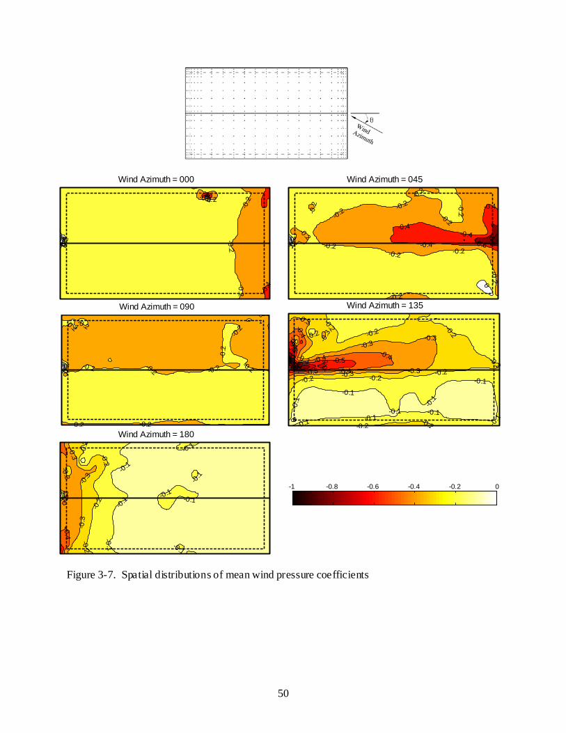
50

-0.4

-0.2

-0.2-0.2

-0.2

0

-0.4

0.2

0.4

Wind Azimuth = 000

-0.8-0.6

-0.4

-0.4-0.4

-0.4

-0.2

-0.2

-0.2-0.2 -0.2

-0.2

-0.2

-0.2

-0.2

-0.2

-0.2

0

0

-0.2

0.2

Wind Azimuth = 045

-0.2 -0.2 -0.2

-0.2

-0.2

-0.2

-0.2-0.2

-0.2-0.2

00.2

Wind Azimuth = 090

-0.7-0.6

-0.5-0.5

-0.5

-0.4

-0.4-0.4

-0.4

-0.3 -0.3

-0.3-0.3

-0.3

-0.3

-0.2 -0.2-0.2

-0.2

-0.2

-0.2-0.2

-0.1

-0.1

-0.1

-0.1

-0.1

-0.1

-0.1-0.1

-0.1

-0.2

-0.2

-0.4

-0.2

-0.8 -0.6

-0.3

0

Wind Azimuth = 135

-0.4

-0.3

-0.3

-0.3-0.2

-0.2

-0.2

-0.2

-0.1

-0.1

-0.1

-0.1

-0.1-0.1

-0.3

-0.1

-0.3

-0.1

Wind Azimuth = 180

-1 -0.8 -0.6 -0.4 -0.2 0

Figure 3-7. Spatial distributions of mean wind pressure coefficients

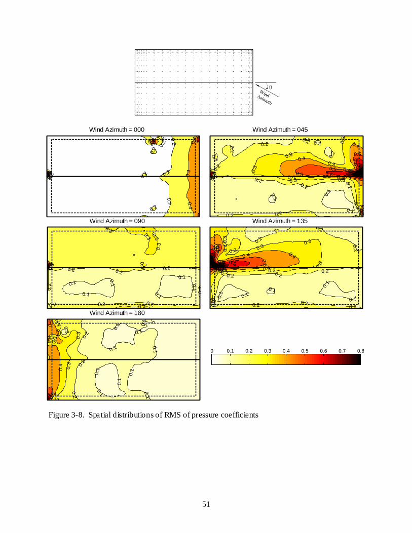
51

0.2

0.2

0.2

0.4

0.4

0.4

0.2

0.20.4

0.2

0.2

0.4

0.2

0.6

0.6

0.2

0.6

1

Wind Azimuth = 000

0.

2

0.2

0.2

0 2

0.20.20.20.2

0.3

0.30.3

0.3

0.30.3

0.3

0.40.4

0.4

0.4

0.4

0.50.5

0.5

0.5

0.1

0.10.2 0.2

0.6

0.6

0.7

0.8

0.2

0.1

0.9

0.4

0.3

0.2

0.4

0.2 0.2

0.5

Wind Azimuth = 045

0.20.20.2

0.2

0.1

0.1

0.1

0.2 0.2 0.2

0.10.10.1

0.3

0.30.3

0.3

0.3

0.3

0.4

0.5

0.3

02

Wind Azimuth = 090

0.2

0.2

0.2

0.20.20.2

0.2

0.2 0.2 0.2

0.3

0.3 0.30.3

0.3

0.30.3

0.3

0.4

0.4 0.4

0.40.4

0.5

0.5

0.5

0.1

0.1

0.60.6

0.10.1

0.70.8

0.1

0.9

0.5 0.4

11

Wind Azimuth = 135

0.1

0.1

0.1

0.1

0.1

0.1

0.1

0.2

0.2

0.2

0.3

0.3

0.3

0.3

0.1

0.1

0.10.

4

0.40.4

0.5

0.2

0.5

0.6

0.3

Wind Azimuth = 180

0 0.1 0.2 0.3 0.4 0.5 0.6 0.7 0.8

Figure 3-8. Spatial distributions of RMS of pressure coefficients

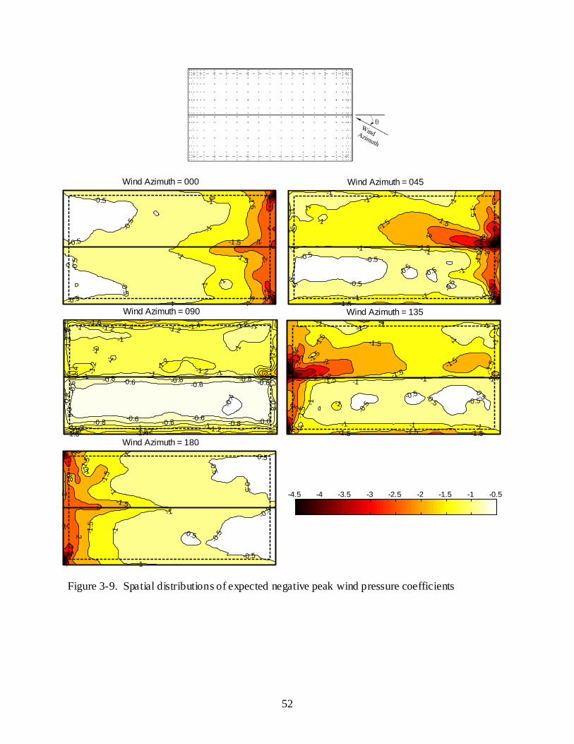
52

-3

-2.5

-2

-2

-2-2

-1.5

-1.5

-1.5

-1.5

-1-1

-1

-1

-1

-0.5

-0.5

-0.5

-0.5

-0.5

-0.5

-1

Wind Azimuth = 000

-3

-3

-2.5-2.5

-2.5-2

-2

-2

-2-2

-1.5

-1.5-1.5

-1.5

-1.5

-1.5

-1.5

-1 -1 -1

-1

-1-1-1

-0.5 -0.5

-0.5-0.5

-1-1

-1-1

-1

-1

-0.5-0.5

-2

-1

-0.5

-1-3

Wind Azimuth = 045

-1.6

-1.6

-1.4 -1.4 -1.4

-1.4-1.4

-1.2

-1.2

-1.2 -1.2 -1.2

-1.2

-1.2-1.2-1.2

-1 -1 -1

-1-1-1-1

-0.8 -0.8 -0.8

-0.8

-0.8-0.8-0.8

-0.8

-0.6 -0.6 -0.6 -0.6

-0.6-0.6-0.6

-0.6

-1

-1-1

-1

-1

-1.2-1.2

-0.4

-1.4

-1-1

Wind Azimuth = 090

-4-3.5

-3

-3

-2.5

-2.5

-2

-2

-2-2

-1.5-1.5-1.5

-1.5

-1.5 -1.5

-1.5-1.5

-1-1-1

-1

-1 -1 -1

-0.5-0.5

-0.5

-1

-1

-1

-1.5

-1.5

-1-1

-0.5

-0.5

-2

-1

-1

-1.5

-1.5

-1

-1Wind Azimuth = 135

-3.5 -3

-2.5-2

-2-2

-2

-1.5

-1.5

-1.5

-1.5

-1

-1

-1

-1-1

-0.5

-0.5

-0.5

-0.5

-0.5

-0.5

-0.5

-2

-1

-2

Wind Azimuth = 180

-4.5 -4 -3.5 -3 -2.5 -2 -1.5 -1 -0.5

Figure 3-9. Spatial distributions of expected negative peak wind pressure coefficients

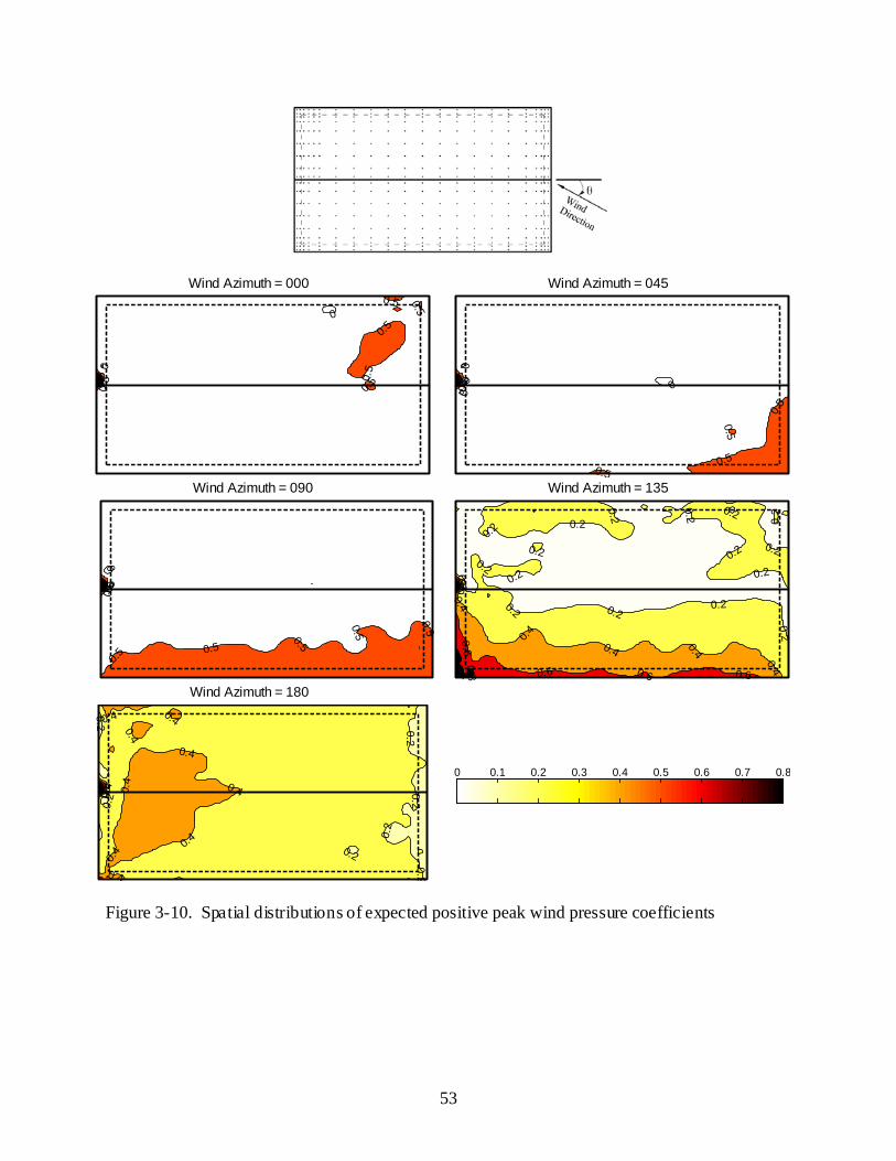
53

0.5

0.5

0.5

0

1 0.5

0.5

2

0.5

0

Wind Azimuth = 000

0.5

0.5

00.51

0.5

0.5

20

0

0

Wind Azimuth = 045

0.5

0.5

0.5

0.5

0.5

0.51

0

2

0

Wind Azimuth = 090

0.2

0.20.2

0.2 0.20.2

0.2

0.4

0.4

0.4 0.4

0.4

0.20.2

0.2

0.2

0.2

0.20.2

0.6

0.6 0.6 0.6

0.8

0.2

0.6

1

0.20.2

1

Wind Azimuth = 135

0.20.2

0.2

0.2

0.2

0.4

0.4

0.4

0.4

0.4

0.4

0.4

0.4

0.4

0.4

0.6

0.2

0.21

Wind Azimuth = 180

0 0.1 0.2 0.3 0.4 0.5 0.6 0.7 0.8

Figure 3-10. Spatial distributions of expected positive peak wind pressure coefficients

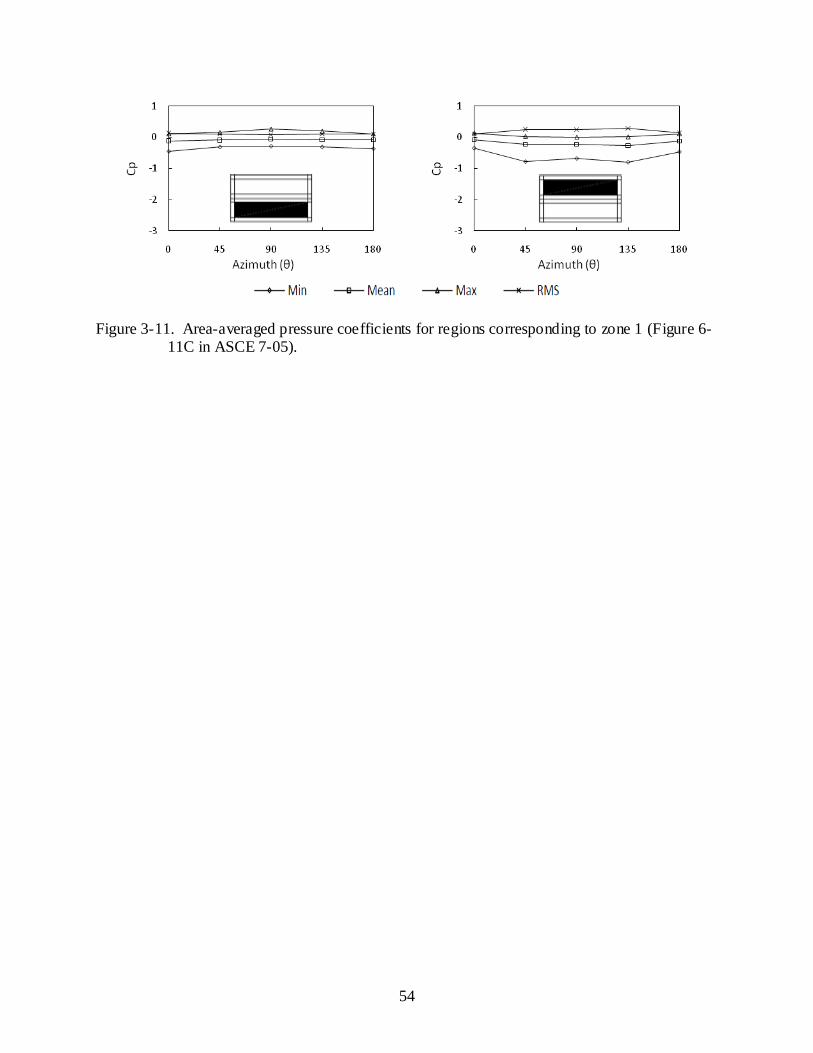
54

Figure 3-11. Area-averaged pressure coefficients for regions corresponding to zone 1 (Figure 6-

11C in ASCE 7-05).

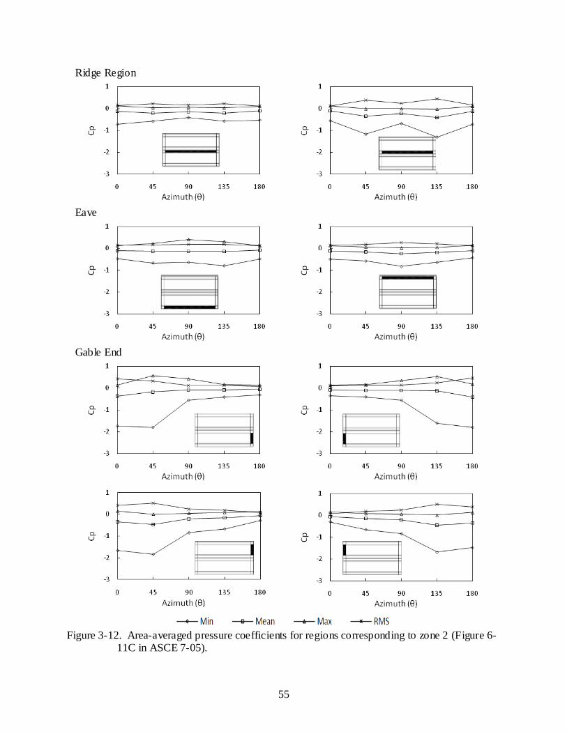
55

Ridge Region

Eave

Gable End

Figure 3-12. Area-averaged pressure coefficients for regions corresponding to zone 2 (Figure 6-11C in ASCE 7-05).

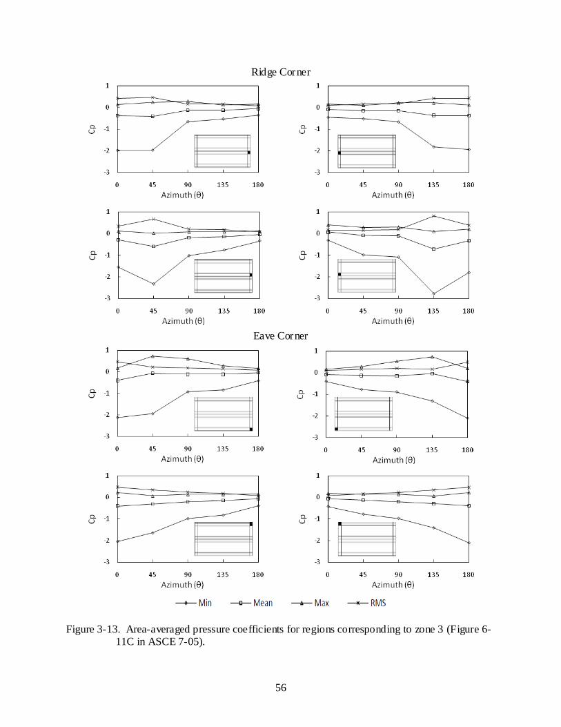
56

Ridge Corner

Eave Corner

Figure 3-13. Area-averaged pressure coefficients for regions corresponding to zone 3 (Figure 6-

11C in ASCE 7-05).

57

CHAPTER 4 APPLICATION OF DAD METHODOLGY

The database-assisted design (DAD) methodo logy utilizes wind-tunnel derived

aerodynamic database of wind pressures in combination with structural influence functions to

predict the wind load e ffects on a structural system.

In this chapter, pressure coefficient time histories developed in Chapter 3 are used with

experimentally derived structural influences to estimate structural reactions at roof-to-wall and

wall-to-foundation connections. This chapter ope ns with an overview of the structural influence

functions which were determined by Datin et al.(2010). A detailed explanation of the app lication

of the DAD approach in this study is provided. Finally, estimated structural reactions, analysis of

results and their comparison with design wind loads based on ASCE 7-05 are presented.

Structural Influence Function

In structural analys is, the variation of shear, reaction, bending moment or de flection in a

structure subjected to live load or moving load is generally best described using an influence line

(Hibbeler 2006). An influence line therefore represents the variation of any structural response at

a specific point in a member as a concentrated force moves over the member. Usually, the

numerical values of a function for an influence line are determined using a dimensionless unit

load. Subsequently the value of a response due to a force applied at any position can be obtained

by multiplying the ordinate of the influence line at that position.

This concept of influence functions is also adopted in the use of the DAD methodology to

predict wind- induced structural responses. For steel framed structures, influence functions used

in DAD-based software provided by NIST(2008) are derived analytically from simple 2D model

of a single frame. However, due to the high variability in wood properties, this study utilizes

58

influence functions determined experimentally on a 1/3-scale wood house model (shown in

Figure 4-1A).

In the experiment, a point load was applied at grid points (shown in figure 4-1C) on the

roo f surface of the mode l house. The reactions induced by the po int loads at 8 roof-to-wall and 9

wall-to-foundation connections were measured by load cells (locations shown in figure 4-1B).

Influence coefficients at each load cell were determined by dividing the measured reactions by

the load applied at the grid points. The resulting fraction (percentage) of the applied load

provides a relative measure of forces transferred to the connections. Structural influence surfaces

over of vertical reactions were generated for each load cell.

To justify the experimental procedure used, s imple 2-D and 3-D models of the building

roof system were analyzed in structural analysis software, ‘Visual Analysis 4.0’. Truss members

were modeled as simply supported beams and were pinned together. For the 3-D model, the roof

sheathing was modeled as a plate element. In both cases, a unit load was applied at points on a

truss of the system and an influence line was drawn for reaction at the truss support. Figure 4-3

shows a comparison of the results with the experimentally derived influence coefficients at grid

points on a truss for a roof-to-wall connection of the truss. Influence function determined by 2D

analytical model decreased linearly with distance between loading point and the support.

However, while the 3D analytical model produced a close agreement with respect to the

variation of influence function as compared to the experimental work, its influence coefficients

differ from experimental results by as much as 30%.

Typical experimentally derived influence surfaces are shown in Figure 4-4.

59

Evaluating Vertical Reactions Based on DAD methodology

Velocity Pressure

Estimates of vertical reactions at the roof-to-wall and wall-to-foundation connections are

based on wind speeds estimates without regard for direction as in the ASCE 7-05 provision.

Velocity pressure, qz (psf) was evaluated at the mean roof height of 14.3 ft as follows:

2,142

1subftairz Vq ρ= (4-1)

openftzsubft VKV ,33,14 =

(4-2)

where ρair is the density of air; Kz is an velocity pressure exposure coefficient whose square root

transforms the 3-second wind speed in miles per hour at 33 ft above ground over open terrain,

V33ft,open into 3-second gust wind speed at mean roof height over a suburban terrain, V14ft,sub.

Kz=0.70 (Table 6-3 o f ASCE 7-05) was used in the DAD approach in order to be consistent with

the ASCE 7 procedure. Also the design wind speed, V33ft,open=130 mph (figure 6-1 o f ASCE 7-05

(2005) was chosen, for consistency with vertical reactions evaluated on the basis of ASCE 7-05.

Hence,

mph8.108)mph130(7.0V sub,ft14 ==

(4-3)

psfmphqz 29.30)8.108(00256.0 2 == (4-4)

Pressure Taps and Influence Functions

The roo f of the prototype house was divided into tributary areas of the pressure taps with

the assumption that pressure coefficient measured by a tap was uniform within its geometric

tributary area. Pressure taps were identified for the influence function grid points which fell

within the tributary of the pressure taps. Consequently, two or more influence coefficients were

60

assigned to a pressure tap and load calculations were based on the tributary area of the influence

function grid point.

Reaction Loads

Reaction time histories at eight roof-to-wall (gable end connection removed) and e leven

wall-to-foundation connections were elevated by “UFDAD” using the wind-tunnel pressure

coefficient time histories and the structural influence functions. The structural loads were

determined by:

[ ]∑=

=1i

ii,pjizj A)t(C)N(q)t(R

(4-5)

where Rj(t) is structural load estimated at jth load cell at time, t; qz is the ve loc ity pressure

evaluated at the mean roof height; Cpi(t) is pressure coefficient for ith gr id point at time t; (Ni)j is

the influence coefficient at the ith grid point for jth load cell; and Ai is the tributary area of ith

grid point.

DAD Results and Analysis

Observed Statistical Values of Structural Reactions

Again, forty files were generated in this analysis each containing s tructural reaction time

histories of the 17 load cells. These times histories are useful in determining peak loads and other

statistical values of interests. They can furthermore be used effectively in probabilistic and

structural reliability studies. Figures 4-6, 4-7 and 4-8 show the time-histories of the vertical

reaction at connections 5, 10 and 15 for wind directions 0o and 45o. The sample mean RMS and

extreme reactions were measured from the time histories for the forty samples of data. The

measured statistical values of reactions for sample 1 are provided in Table 4-1.The statistical

values for the other samples are provided in Appendix B.

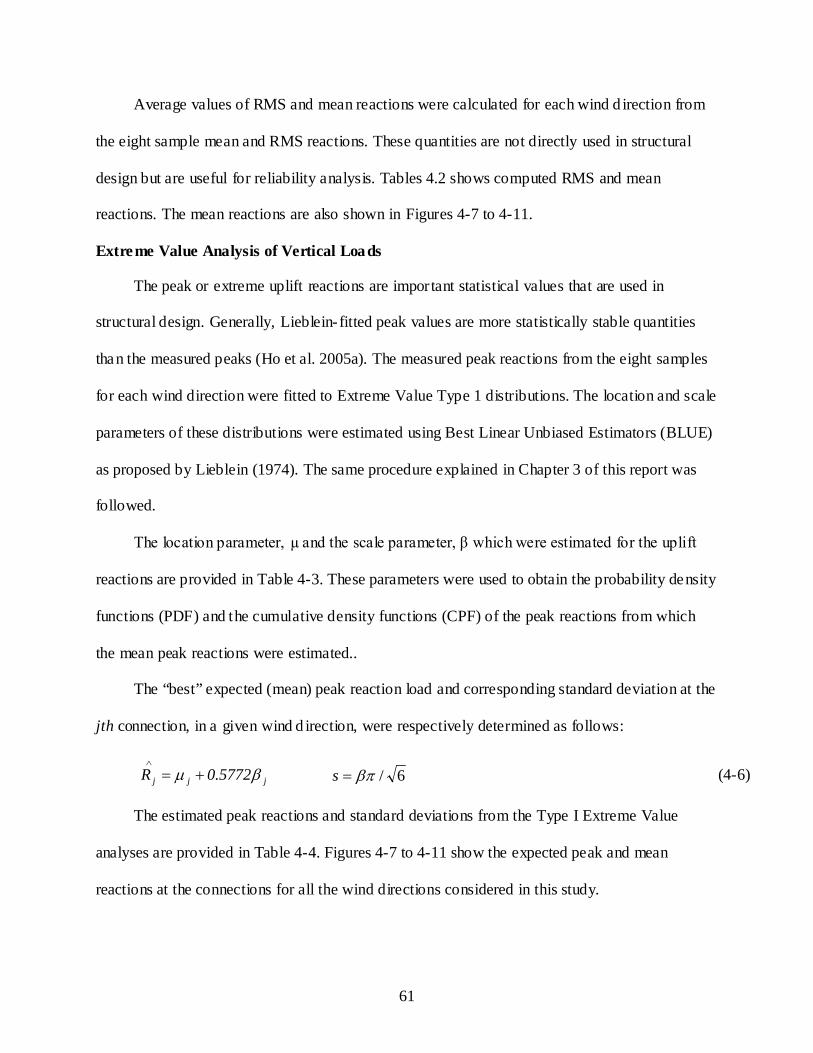
61

Average values of RMS and mean reactions were calculated for each wind d irection from

the eight sample mean and RMS reactions. These quantities are not directly used in structural

design but are useful for reliability analysis. Tables 4.2 shows computed RMS and mean

reactions. The mean reactions are also shown in Figures 4-7 to 4-11.

Extreme Value Analysis of Vertical Loads

The peak or extreme uplift reactions are important statistical values that are used in

structural design. Generally, Lieblein-fitted peak values are more statistically stable quantities

than the measured peaks (Ho et al. 2005a). The measured peak reactions from the eight samples

for each wind direction were fitted to Extreme Value Type 1 distributions. The location and scale

parameters of these distributions were estimated using Best Linear Unbiased Estimators (BLUE)

as proposed by Lieblein (1974). The same procedure explained in Chapter 3 of this report was

followed.

The location parameter, µ and the scale parameter, β which were estimated for the uplift

reactions are provided in Table 4-3. These parameters were used to obtain the probability density

functions (PDF) and the cumulative density functions (CPF) of the peak reactions from which

the mean peak reactions were estimated..

The “best” expected (mean) peak reaction load and corresponding standard deviation at the

jth connection, in a given wind d irection, were respectively determined as follows:

jjj 5772.0R βµ +=∧

6/βπ=s (4-6)

The estimated peak reactions and standard deviations from the Type I Extreme Value

analyses are provided in Table 4-4. Figures 4-7 to 4-11 show the expected peak and mean

reactions at the connections for all the wind directions considered in this study.

62

It is observed from the plots that, a greater percentage of the uplift loads were transferred

through the roof-to-wall connections (load cells 15 and 19) at the gable end. The highest uplift

reaction (1750 lbs) estimated was transferred through load cell 15 for wind directions 0o and 45o.

It is worth nothing that, the influence coefficients for this connection are higher at the gable edge

and the ridge corners, where high suctions were observed. Again its influence surface was wide

spread than in the case of the other roof-to-wall connections.

Again, though the connections between the gable end roof and wall were discontinued

except at the end connections, reasonable uplift loads are transferred through foundation load

cells 11, 12 and 13 for the directions. This is explained by the widespread of their influence

surfaces as a result of the diaphragm action in the wall (similar to deep beam action). However,

very small loads are transferred through load cell 14.

Relatively higher uplift loads were estimated at all connections for wind direction 0o than

the other azimuths. The loads generally decreased as the direction of the incident increased.

Higher positive reactions were transferred through the load cells for wind azimuth 90o because

peak positive pressures enveloped the building for that wind direction.

Vertical Reaction Based on ASCE 7-05 S tandard

ASCE 7-05 provides separate provisions for wind design using loads for either the main

wind force resisting system (MWFRS) or for components and cladding (C&C) members. Major

members of a building, which work together with other members in an assemblage to provide

support and stability for the overall building, are designed using wind loads provided for

MWFRS. Other members, which are directly loaded, are designed for localized wind load effects

on relatively small areas using provisions for C&C.

Roof-to-wall connections (truss reactions) which serve as media for transfer of wind

loading on the roof system to walls have in the past (Datin and Prevatt 2007) been designed as

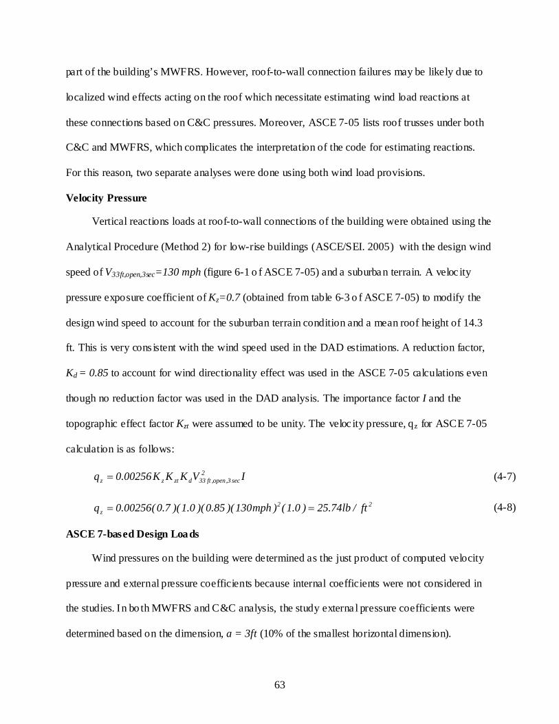
63

part of the building’s MWFRS. However, roof-to-wall connection failures may be likely due to

localized wind effects acting on the roof which necessitate estimating wind load reactions at

these connections based on C&C pressures. Moreover, ASCE 7-05 lists roof trusses under both

C&C and MWFRS, which complicates the interpretation of the code for estimating reactions.

For this reason, two separate analyses were done using both wind load provisions.

Velocity Pressure

Vertical reactions loads at roof-to-wall connections of the building were obtained using the

Analytical Procedure (Method 2) for low-rise buildings (ASCE/SEI. 2005) with the design wind

speed of V33ft,open,3sec=130 mph (figure 6-1 o f ASCE 7-05) and a suburban terrain. A veloc ity

pressure exposure coefficient of Kz=0.7 (obtained from table 6-3 o f ASCE 7-05) to modify the

design wind speed to account for the suburban terrain condition and a mean roof height of 14.3

ft. This is very cons istent with the wind speed used in the DAD estimations. A reduction factor,

Kd = 0.85 to account for wind directionality effect was used in the ASCE 7-05 calculations even

though no reduction factor was used in the DAD analysis. The importance factor I and the

topographic effect factor Kzt were assumed to be unity. The veloc ity pressure, qz for ASCE 7-05

calculation is as follows:

IVKKK00256.0q 2sec3,open,ft33dztzz = (4-7)

22z ft/lb74.25)0.1()mph130)(85.0)(0.1)(7.0(00256.0q == (4-8)

ASCE 7-based Design Loads

Wind pressures on the building were determined as the just product of computed velocity

pressure and external pressure coefficients because internal coefficients were not considered in

the studies. In bo th MWFRS and C&C analysis, the study externa l pressure coefficients were

determined based on the dimension, a = 3ft (10% of the smallest horizontal dimension).

64

For ASCE 7-05 MWFRS, external pressure coefficients are defined with respect to roo f

angles and building surfaces. The building has a roof angle of 18.4o and therefore linear

interpolations were used to determine external pressure coefficients. Partitioning of the roof

surface into four building surfaces as defined in Figure 6-10 of ASCE 7-05 is shown in Figure 4-

12. Partitions were used to determine the pressures on the individual trusses. Table 4-5 shows

MWFRS based wind pressures for the different building surface based on the velocity pressure.

In the case of C&C, external pressure coefficients were obtained from Figure 6-11C of the

ASCE 7-05. Selection of the coefficients was based on an effective wind area of 300 ft2, which is

a product of 30 ft span length and one-third the span length. The building roof surface again, was

partitioned into pressures zones as de fined in ASCE 7 (see Figure 4-13). Wind Pressures based

on C&C provisions for the zones including the roof overhang as given in Table 4-6.

Wind load intensity on each truss was calculated by multiplying pressure on the truss

tributary area by its tributary width. Each truss was loaded with its pressure intensity and

analyzed separately in “Visual Analysis 4.0” to determine the structural reaction at its support,

for both MWFRS and C&C cases. For MWFRS case, the procedure was repeated for all the eight

load patterns defined in Figure 6-10 in ASCE 7 to obtain the maximum uplift reaction.

Comparing Uplifts Reactions Predicted Based on DAD vs. ASCE 7-05

For comparison, the DAD-based reactions results were multiplied by 0.85 to account for

the reduced probability of maximum winds coming from any direction, as it was in the case of

the ASCE 7-based estimations. The worst uplift loads estimated at each of the roof to wall

connections were selected and compared to the peak estimates based on the ASCE 7 Standard for

MWFRS and Components and Cladding (C&C).

The comparison of the results based on ASCE 7-05 and DAD methodology are presented

in Table 4-7. The results are graphically presented in Figure 4-13.

65

It is observed that the DAD-based reactions are generally higher than reactions based on

ASCE 7-05 MWFRS provisions. At the gable end supports, ASCE 7 MWFRS underestimate the

reaction at that support by as much as 28 % as compared to the DAD estimates.

Underestimations of reactions by ASCE 7 MWFRS provisions are high at truss supports closer to

the gable end o f the house. Very close results are however observed between the results at truss

suppo rts which are far away from the gable end.

Significantly high reactions (by 6% to 62%) are observed for reactions based on ASCE 7-

C&C than in the case of the DAD. Using discrepancies observed in the two comparisons above,

the DAD results have a better agreement with ASCE 7 MWFRS estimates than C&C based

estimates.

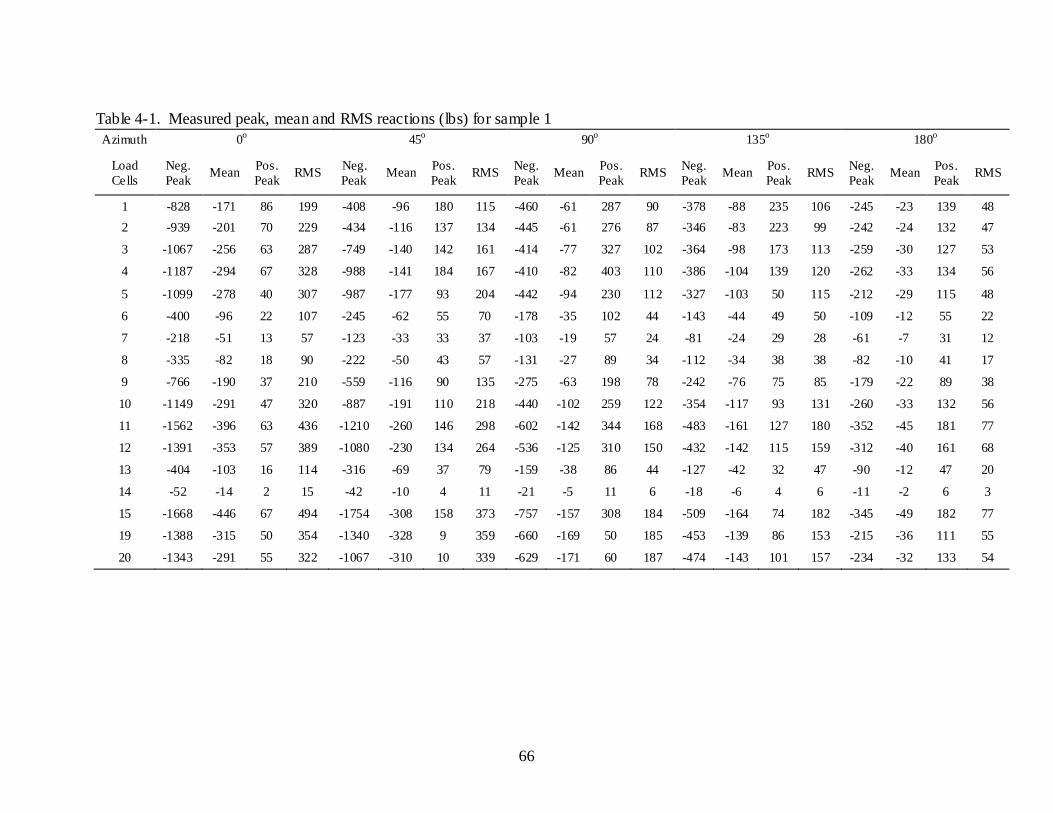
66

Table 4-1. Measured peak, mean and RMS reactions (lbs) for sample 1 Azimuth 0o 45o 90o 135o 180o

Load Cells

Neg. Peak Mean Pos.

Peak RMS Neg. Peak Mean Pos.




Peak RMS

1 -828 -171 86 199 -408 -96 180 115 -460 -61 287 90 -378 -88 235 106 -245 -23 139 48 2 -939 -201 70 229 -434 -116 137 134 -445 -61 276 87 -346 -83 223 99 -242 -24 132 47

3 -1067 -256 63 287 -749 -140 142 161 -414 -77 327 102 -364 -98 173 113 -259 -30 127 53

4 -1187 -294 67 328 -988 -141 184 167 -410 -82 403 110 -386 -104 139 120 -262 -33 134 56

5 -1099 -278 40 307 -987 -177 93 204 -442 -94 230 112 -327 -103 50 115 -212 -29 115 48

6 -400 -96 22 107 -245 -62 55 70 -178 -35 102 44 -143 -44 49 50 -109 -12 55 22

7 -218 -51 13 57 -123 -33 33 37 -103 -19 57 24 -81 -24 29 28 -61 -7 31 12

8 -335 -82 18 90 -222 -50 43 57 -131 -27 89 34 -112 -34 38 38 -82 -10 41 17

9 -766 -190 37 210 -559 -116 90 135 -275 -63 198 78 -242 -76 75 85 -179 -22 89 38

10 -1149 -291 47 320 -887 -191 110 218 -440 -102 259 122 -354 -117 93 131 -260 -33 132 56

11 -1562 -396 63 436 -1210 -260 146 298 -602 -142 344 168 -483 -161 127 180 -352 -45 181 77

12 -1391 -353 57 389 -1080 -230 134 264 -536 -125 310 150 -432 -142 115 159 -312 -40 161 68

13 -404 -103 16 114 -316 -69 37 79 -159 -38 86 44 -127 -42 32 47 -90 -12 47 20

14 -52 -14 2 15 -42 -10 4 11 -21 -5 11 6 -18 -6 4 6 -11 -2 6 3

15 -1668 -446 67 494 -1754 -308 158 373 -757 -157 308 184 -509 -164 74 182 -345 -49 182 77

19 -1388 -315 50 354 -1340 -328 9 359 -660 -169 50 185 -453 -139 86 153 -215 -36 111 55

20 -1343 -291 55 322 -1067 -310 10 339 -629 -171 60 187 -474 -143 101 157 -234 -32 133 54

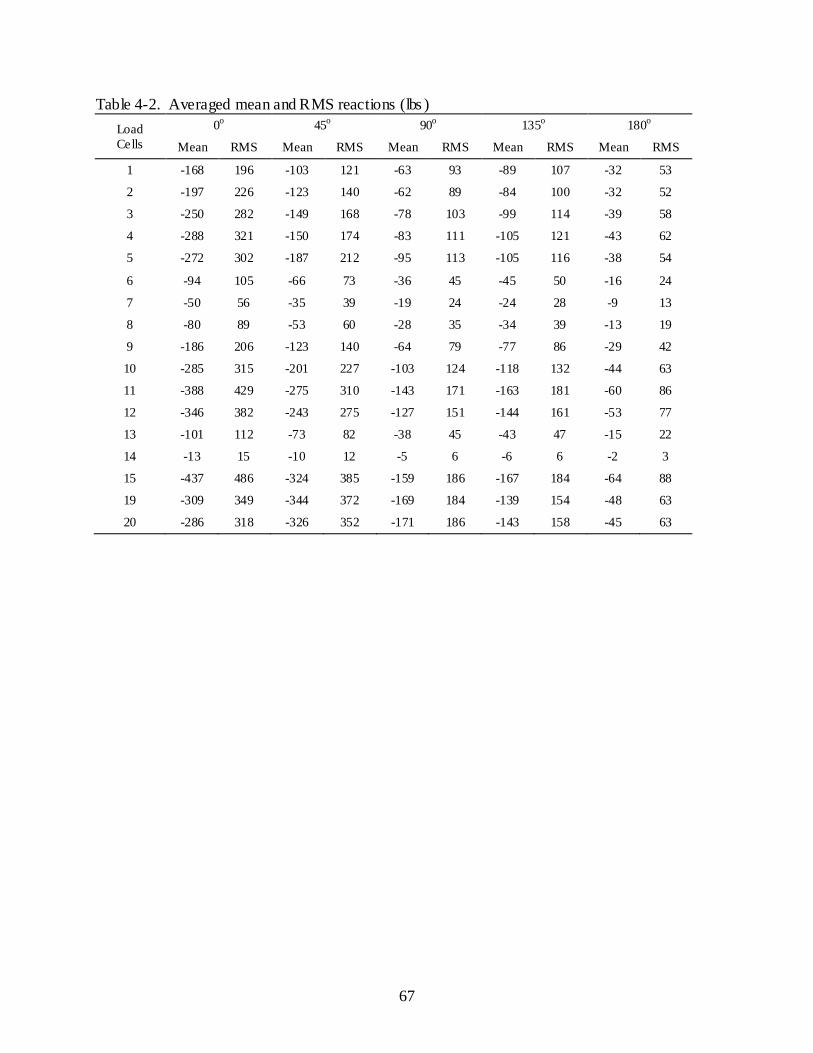
67

Table 4-2. Averaged mean and RMS reactions (lbs ) Load Cells

0o 45o 90o 135o 180o

Mean RMS Mean RMS Mean RMS Mean RMS Mean RMS

1 -168 196 -103 121 -63 93 -89 107 -32 53

2 -197 226 -123 140 -62 89 -84 100 -32 52

3 -250 282 -149 168 -78 103 -99 114 -39 58

4 -288 321 -150 174 -83 111 -105 121 -43 62

5 -272 302 -187 212 -95 113 -105 116 -38 54

6 -94 105 -66 73 -36 45 -45 50 -16 24

7 -50 56 -35 39 -19 24 -24 28 -9 13

8 -80 89 -53 60 -28 35 -34 39 -13 19

9 -186 206 -123 140 -64 79 -77 86 -29 42

10 -285 315 -201 227 -103 124 -118 132 -44 63

11 -388 429 -275 310 -143 171 -163 181 -60 86

12 -346 382 -243 275 -127 151 -144 161 -53 77

13 -101 112 -73 82 -38 45 -43 47 -15 22

14 -13 15 -10 12 -5 6 -6 6 -2 3

15 -437 486 -324 385 -159 186 -167 184 -64 88

19 -309 349 -344 372 -169 184 -139 154 -48 63

20 -286 318 -326 352 -171 186 -143 158 -45 63

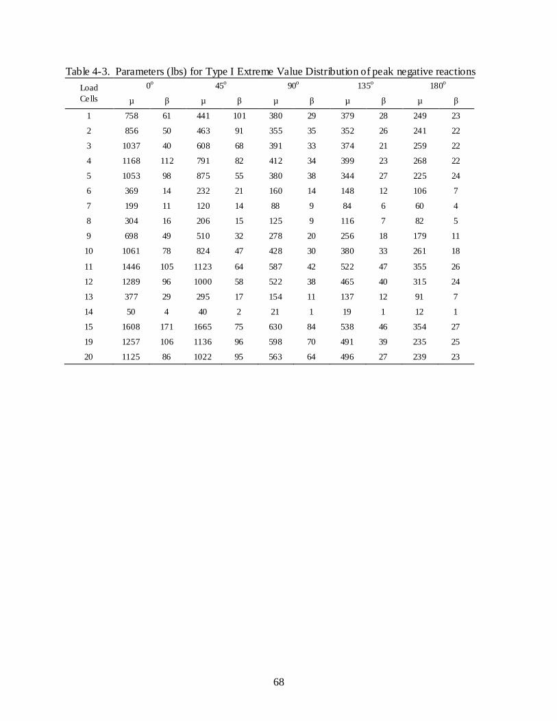
68

Table 4-3. Parameters (lbs) for Type I Extreme Value Distribution of peak negative reactions Load Cells

0o 45o 90o 135o 180o

µ β µ β µ β µ β µ β

1 758 61 441 101 380 29 379 28 249 23

2 856 50 463 91 355 35 352 26 241 22

3 1037 40 608 68 391 33 374 21 259 22

4 1168 112 791 82 412 34 399 23 268 22

5 1053 98 875 55 380 38 344 27 225 24

6 369 14 232 21 160 14 148 12 106 7

7 199 11 120 14 88 9 84 6 60 4

8 304 16 206 15 125 9 116 7 82 5

9 698 49 510 32 278 20 256 18 179 11

10 1061 78 824 47 428 30 380 33 261 18

11 1446 105 1123 64 587 42 522 47 355 26

12 1289 96 1000 58 522 38 465 40 315 24

13 377 29 295 17 154 11 137 12 91 7

14 50 4 40 2 21 1 19 1 12 1

15 1608 171 1665 75 630 84 538 46 354 27

19 1257 106 1136 96 598 70 491 39 235 25

20 1125 86 1022 95 563 64 496 27 239 23

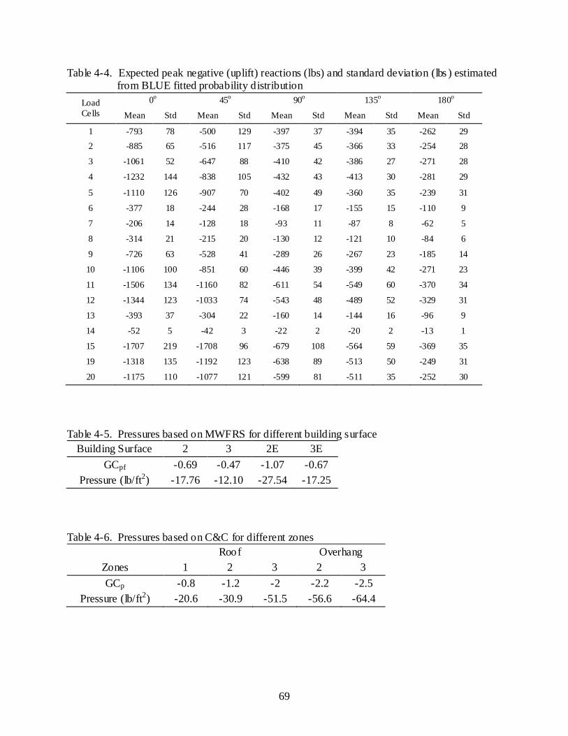
69

Table 4-4. Expected peak negative (uplift) reactions (lbs) and standard deviation (lbs ) estimated from BLUE fitted probability distribution

Load Cells

0o 45o 90o 135o 180o

Mean Std Mean Std Mean Std Mean Std Mean Std

1 -793 78 -500 129 -397 37 -394 35 -262 29 2 -885 65 -516 117 -375 45 -366 33 -254 28

3 -1061 52 -647 88 -410 42 -386 27 -271 28

4 -1232 144 -838 105 -432 43 -413 30 -281 29

5 -1110 126 -907 70 -402 49 -360 35 -239 31

6 -377 18 -244 28 -168 17 -155 15 -110 9

7 -206 14 -128 18 -93 11 -87 8 -62 5

8 -314 21 -215 20 -130 12 -121 10 -84 6

9 -726 63 -528 41 -289 26 -267 23 -185 14

10 -1106 100 -851 60 -446 39 -399 42 -271 23

11 -1506 134 -1160 82 -611 54 -549 60 -370 34

12 -1344 123 -1033 74 -543 48 -489 52 -329 31

13 -393 37 -304 22 -160 14 -144 16 -96 9

14 -52 5 -42 3 -22 2 -20 2 -13 1

15 -1707 219 -1708 96 -679 108 -564 59 -369 35

19 -1318 135 -1192 123 -638 89 -513 50 -249 31

20 -1175 110 -1077 121 -599 81 -511 35 -252 30

Table 4-5. Pressures based on MWFRS for different building surface Building Surface 2 3 2E 3E

GCpf -0.69 -0.47 -1.07 -0.67 Pressure (lb/ft2) -17.76 -12.10 -27.54 -17.25

Table 4-6. Pressures based on C&C for different zones Roof Overhang

Zones 1 2 3 2 3 GCp -0.8 -1.2 -2 -2.2 -2.5

Pressure (lb/ft2) -20.6 -30.9 -51.5 -56.6 -64.4

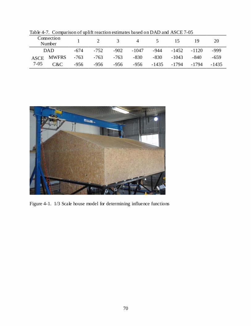
70

Table 4-7. Comparison of uplift reaction estimates based on DAD and ASCE 7-05 Connection

Number 1 2 3 4 5 15 19 20

DAD -674 -752 -902 -1047 -944 -1452 -1120 -999 ASCE 7-05

MWFRS -763 -763 -763 -830 -830 -1043 -840 -659 C&C -956 -956 -956 -956 -1435 -1794 -1794 -1435

Figure 4-1. 1/3 Scale house model for determining influence functions

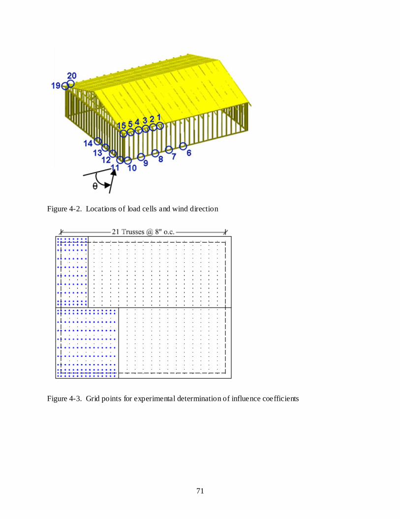
71

Figure 4-2. Locations of load cells and wind direction

Figure 4-3. Grid points for experimental determination of influence coefficients

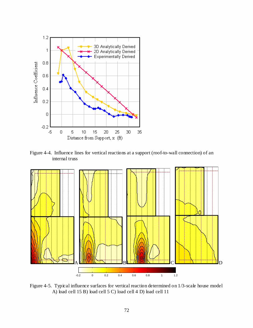
72

Figure 4-4. Influence lines for vertical reactions at a support (roof-to-wall connection) of an

internal truss

A

B

C

D

-0.2 0 0.2 0.4 0.6 0.8 1 1.2

Figure 4-5. Typical influence surfaces for vertical reaction determined on 1/3-scale house model

A) load cell 15 B) load cell 5 C) load cell 4 D) load cell 11

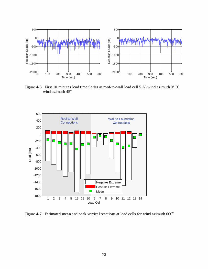
73

0 100 200 300 400 500 600-2000

-1500

-1000

-500

0

500R

eact

ion

Load

s (lb

s)

Time (sec) 0 100 200 300 400 500 600

-2000

-1500

-1000

-500

0

500

Rea

ctio

n Lo

ads

(lbs)

Time (sec) Figure 4-6. First 10 minutes load time Series at roof-to-wall load cell 5 A) wind azimuth 0o B)

wind azimuth 45o

1 2 3 4 5 15 19 20 6 7 8 9 10 11 12 13 14-1800

-1600

-1400

-1200

-1000

-800

-600

-400

-200

0

200

400

600

Load

(lbs

)

Load Cell

Negative ExtremePositive ExtremeMean

Roof-to-WallConnections

Wall-to-FoundationConnections

Figure 4-7. Estimated mean and peak vertical reactions at load cells for wind azimuth 000o

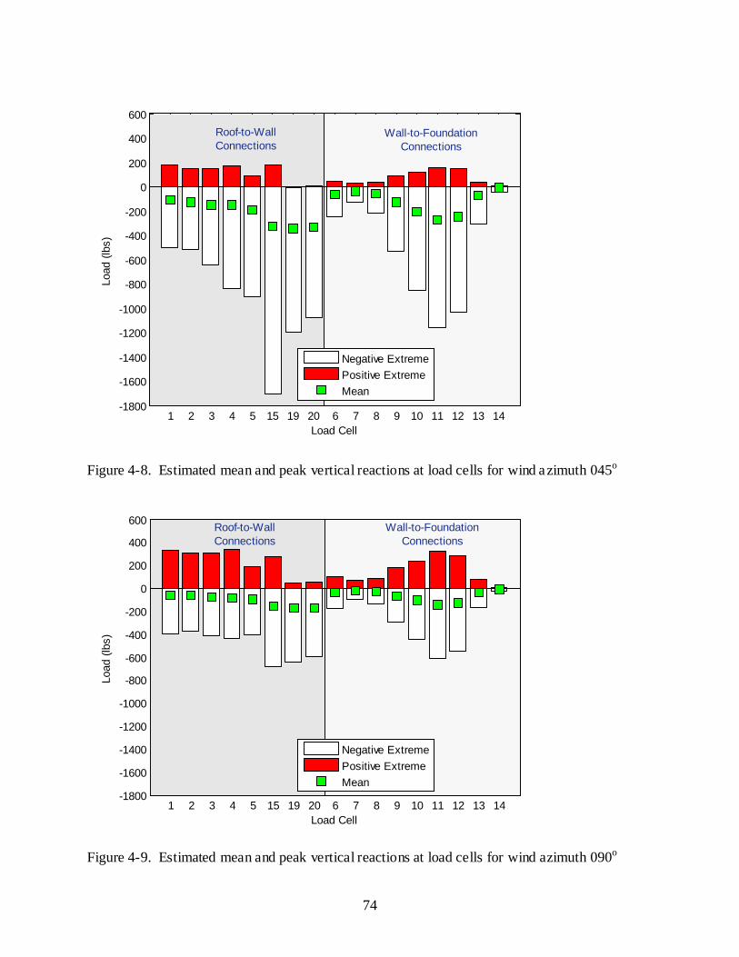
74

1 2 3 4 5 15 19 20 6 7 8 9 10 11 12 13 14-1800

-1600

-1400

-1200

-1000

-800

-600

-400

-200

0

200

400

600Lo

ad (l

bs)

Load Cell





1 2 3 4 5 15 19 20 6 7 8 9 10 11 12 13 14-1800

-1600

-1400

-1200

-1000

-800

-600

-400

-200

0

200

400

600

Load

(lbs

)

Load Cell





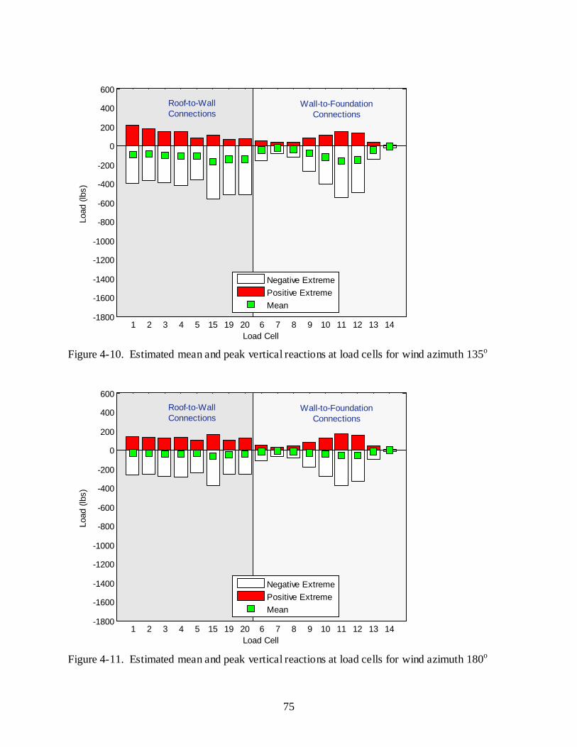
75

1 2 3 4 5 15 19 20 6 7 8 9 10 11 12 13 14-1800

-1600

-1400

-1200

-1000

-800

-600

-400

-200

0

200

400

600Lo

ad (l

bs)

Load Cell





1 2 3 4 5 15 19 20 6 7 8 9 10 11 12 13 14-1800

-1600

-1400

-1200

-1000

-800

-600

-400

-200

0

200

400

600

Load

(lbs

)

Load Cell





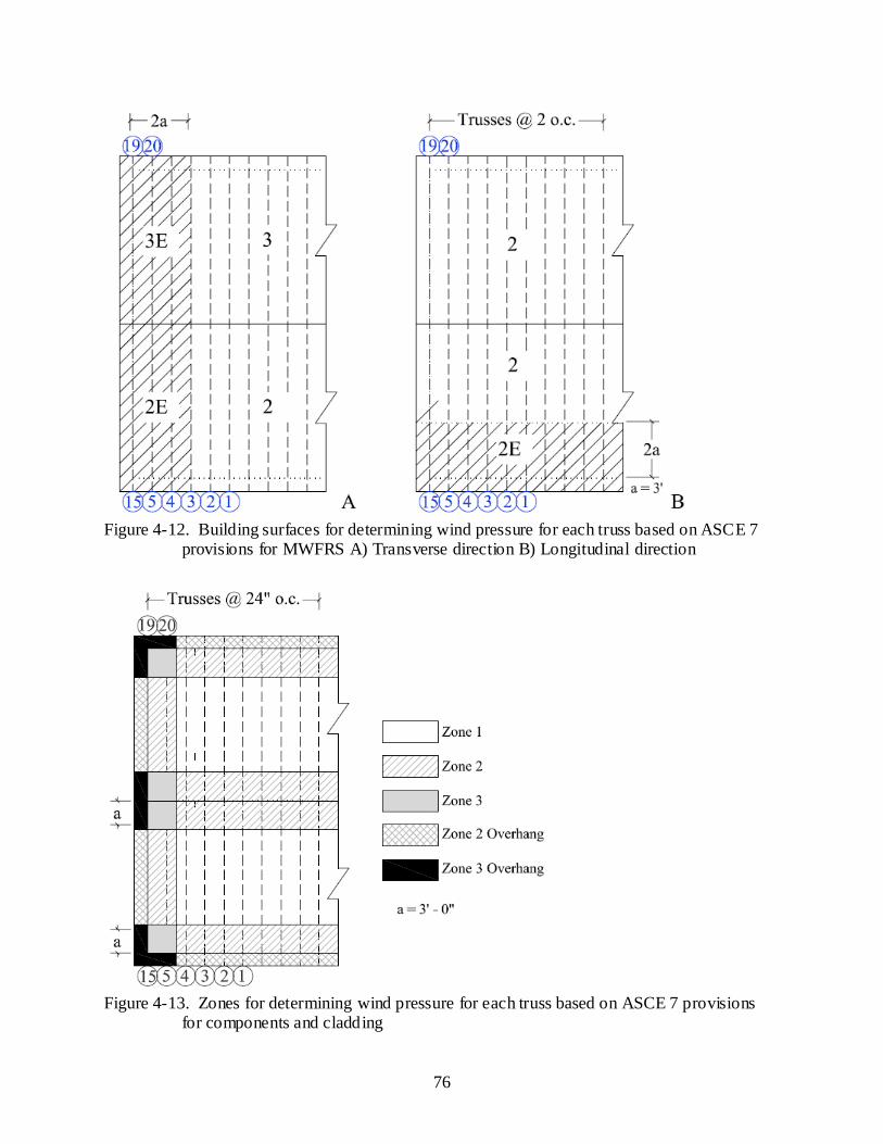
76

Figure 4-12. Building surfaces for determining wind pressure for each truss based on ASCE 7

provisions for MWFRS A) Transverse direction B) Longitudinal direction

Figure 4-13. Zones for determining wind pressure for each truss based on ASCE 7 provisions

for components and cladding

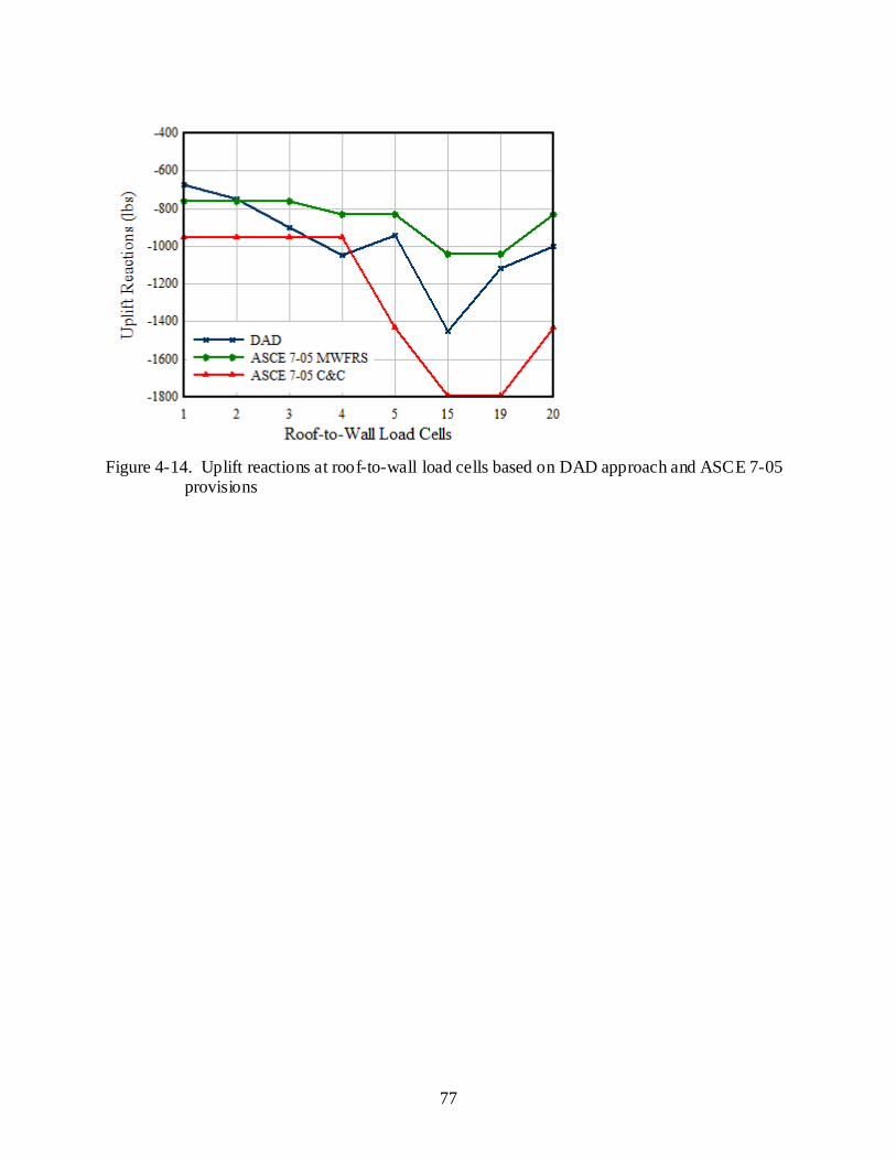
77

Figure 4-14. Uplift reactions at roof-to-wall load cells based on DAD approach and ASCE 7-05

provisions

78

CHAPTER 5 WIND FLOW CHARACTERIZATION USING TFI COBRA PROBE

The flow characteristics of wind largely influence the intensity and fluctuation of wind

forces on structures. The experimental component of the study includes a scale house mode l

immersed within a wind flow generated by a UF Wind Generator. A multi-hole pressure probe

called the Cobra Probe was used to map the wind flow characteristics to provide the necessary

information for analyzing the data.

This chapter discusses the Cobra Probe, its principle of operation and pilot flow

measurements conducted prior to using it in the main experimental study. Flow characterization

of the wind field produced for the experiment is also presented in this chapter.

The Cobra Probe

The Cobra Probe (shown in Figure 5-1A) is a robust and compact multi-hole pressure

probe designed by Turbulent Flow Instrumentation (TFI), Australia, for measuring turbulent

wind flows. The Cobra probe was first proposed by Shepherd (1981) for mean flow

measurements and further developed by Hooper and Musgrove (1997) for resolving turbulence

structure. The device has the following advantages:

1. It resolves highly turbulent wind flows into three orthogonal components at high frequency (up to 10000 Hz).

2. It is a robust self contained device.

3. It can withstand significant levels of instrument vibration and maintain accuracy (Watkins et al. 2004).

The high sampling frequency of the probe allows for continuous data streaming, with

virtually unlimited data to be recorded while avoiding aliasing and reducing measurement of

noise. The Probe has a truncated triangular pyramid-shaped head with four faces ground flat to

45o (Chen et al. 2000). Each face has a 0.5 mm diameter pressure tap located at its center that is

79

connected to piezo-resistive bridge pressure transducers, and a preamplifier system located

within the body of the probe. This arrangement was necessary to minimize the lengt h of tubing

so as to achieve a high frequency response as well as mechanically protecting the transducers.

The probe has an overall length of 160 mm and a body diameter of 14 mm. The design of the

probe is shown in Figure 5-1B.

The principle of operation of the probe is to relate the pressure field detected by four

pressure transducers to the magnitude of the instantaneous local veloc ity vector, yaw and pitch

angles and the instantaneous static pressure. Pressure signa ls measured are corrected for

transmission effects, using a predetermined transfer function (frequency response func tion) of

pressure tubing (Chen et al. 2000).

A Series 100 Cobra Probe (Serial ID 193) was used in the study. It has a veloc ity range of

3 m/s to 60 m/s and an accuracy of 0.5±m/s and was supplied with an interface unit housing an

integrated data acquisition and device control software.

Preliminary Experiments Using the Cobra Probe

Pilot experiments were conducted using the Cobra Probe aimed at (1) comparing flow

measurements by the probe and hotwire anemometer (b) understanding the use and principle of

the probe and (3) evaluating methods in modeling flow field conditions for the study’s main

experiment.

In all the preliminary experiments, flow measurements were usually sampled by the probe

at 5000 Hz and down sampled at a rate of 2500 Hz for 120 seconds per each test run. Before

each test, the probe was zeroed to remove offset voltages from its pressure transducers.

Comparing Wind Flow Measurements by the Cobra Probe and Hotwire Anemometer

Flow measurements were simultaneously taken by the cobra probe and a hot-wire

anemometer in a generated wind field. Table 5-1 compares the mean axial velocities, U, and

80

turbulence intensities, Iuu, measured by the Cobra Probe and the hot-wire anemometer. Good

agreement is observed for the mean velocities. However, significant differences are observed for

the turbulence intensities, which may in part be due to errors as a result of relative positions of

the instruments.

Wind Tunnel Model

Several tests were done in a small wind tunnel (shown in Figure 5-3) to understand the

principle and usage of the probe. The wind tunnel consists of a 10 ft long test section, a

contraction area, and a plenum and flow straighter section. It is powered by a 2 ft diameter axial

fan. The test section is 24 in wide and 8 in high.

Results from one test where flow measurements were taken at points (shown in Figure 5-

4) within a 2D surface at 0.5 in downstream of the wind tunnel exit are presented. Profiles for all

the orthogonal mean veloc ities measured a re shown in Figure 5-5. Corresponding turbulence

intensity distributions for longitudinal (Iuu), transverse (Ivv) and vertical (Iww) directions of flow

are also displayed in Figure 5-5B. It is seen from the plots that very low transverse and vertical

wind velocities are recorded away from the walls as compared to the high axial velocities.

Relatively low axial velocities with corresponding high turbulent intensities are observed near

the wall surfaces of the test section. This is due to a high frictional effect near the wall surfaces.

Figures 5-6 to 5-8 show the 2D variation of the mean velocities and turbulent intensities across

the test section. The spectral contents of wind speeds at the exit of the wind tunnel are displayed

in Figure 5-9.

Mapping o f Wind Field Generated by UF Wind Generator

Veloc ity and turbulent intensity measurements of the wind flow generated by the UF wind

generator were taken prior to this study’s experimental work. The main purpose was to

investigate if the wind field was uniform within the test area.

81

The probe was mounted on a computer-controlled traverse to control the horizontal

position. Vertical adjustments of the probe were done manually. The traverse frame was set up in

two locations laterally to map the wind flow across the section. Figure 5-10 shows the traverse

frame within the test area.

The Cobra Probe was used to measure flow characteristics at 90 locations (shown in

Figure 5-11) within a cross-section at 16 ft downstream of the wind generator. Each

measurement was taken for 60 seconds at a sampling frequency of 10000 Hz and output to file at

5000 Hz. A mean wind velocity of 50 mph (22 m/s) was used for all the tests.

Contour plots of longitudinal, transverse and vertical wind fields are shown in Figures 5-

12 and 5-13. Relatively low longitudinal wind speeds at locations outside the jet field were

observed. Longitudinal wind speed was generally uniform across the cross-section but decrease

near the wall.

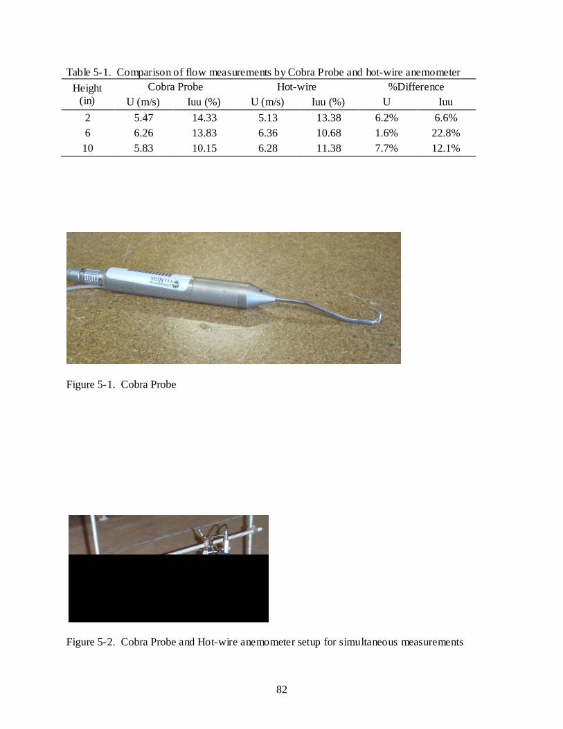
82

Table 5-1. Comparison of flow measurements by Cobra Probe and hot-wire anemometer Height

(in) Cobra Probe Hot-wire %Difference

U (m/s) Iuu (%) U (m/s) Iuu (%) U Iuu 2 5.47 14.33 5.13 13.38 6.2% 6.6% 6 6.26 13.83 6.36 10.68 1.6% 22.8% 10 5.83 10.15 6.28 11.38 7.7% 12.1%

Figure 5-1. Cobra Probe

Figure 5-2. Cobra Probe and Hot-wire anemometer setup for simultaneous measurements

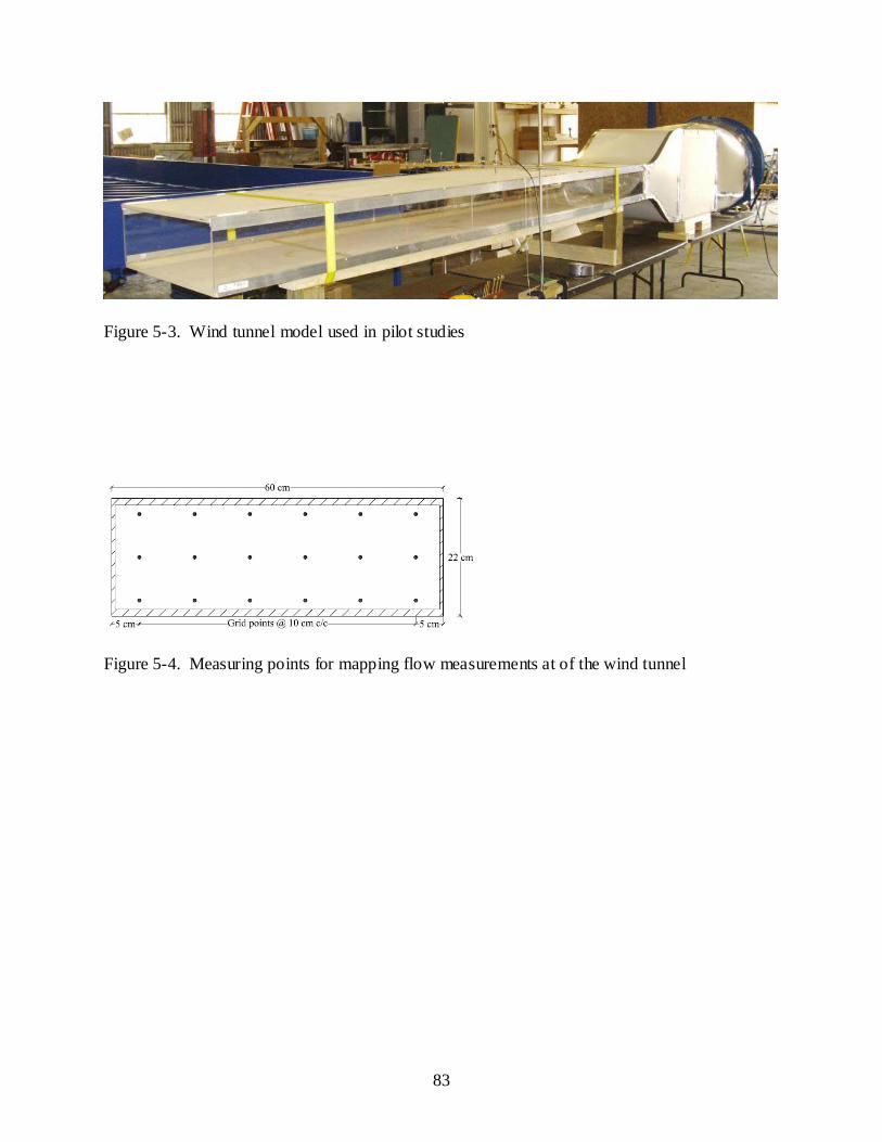
83

Figure 5-3. Wind tunnel model used in pilot studies

Figure 5-4. Measuring points for mapping flow measurements at of the wind tunnel

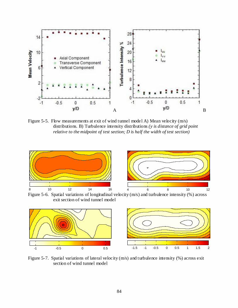
84

A B Figure 5-5. Flow measurements at exit of wind tunnel model A) Mean velocity (m/s)

distributions. B) Turbulence intensity distributions (y is distance of grid point relative to the midpoint of test section; D is half the width of test section)

8 10 12 14 16

4 6 8 10 12 Figure 5-6. Spatial variations of longitudinal velocity (m/s) and turbulence intensity (%) across

exit section of wind tunnel model

-1 -0.5 0 0.5

-1.5 -1 -0.5 0 0.5 1 1.5 2 Figure 5-7. Spatial variations of lateral velocity (m/s) and turbulence intensity (%) across exit

section of wind tunnel model

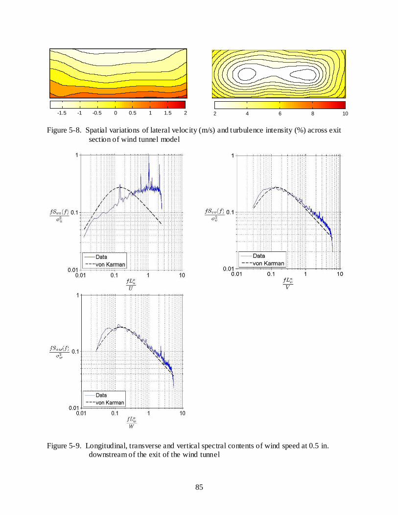
85

-1.5 -1 -0.5 0 0.5 1 1.5 2

2 4 6 8 10 Figure 5-8. Spatial variations of lateral velocity (m/s) and turbulence intensity (%) across exit

section of wind tunnel model

Figure 5-9. Longitudinal, transverse and vertical spectral contents of wind speed at 0.5 in.

downstream of the exit of the wind tunnel

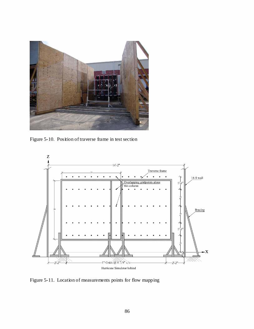
86

Figure 5-10. Position of traverse frame in test section

Figure 5-11. Location of measurements points for flow mapping

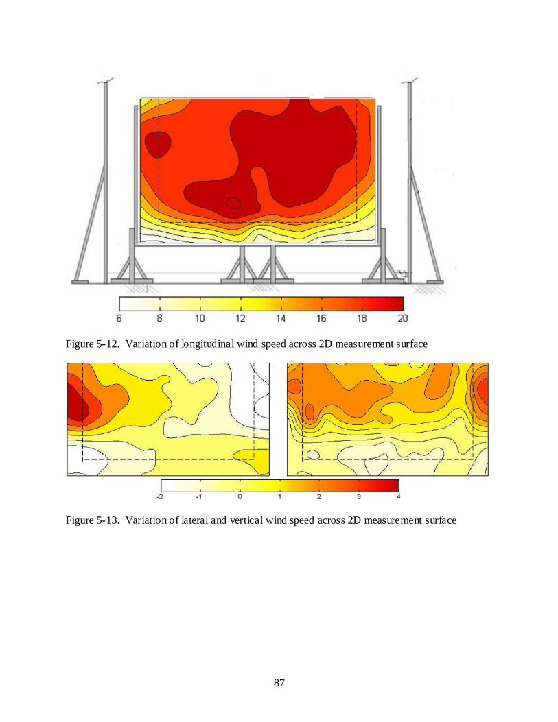
87

Figure 5-12. Variation of longitudinal wind speed across 2D measurement surface

Figure 5-13. Variation of lateral and vertical wind speed across 2D measurement surface

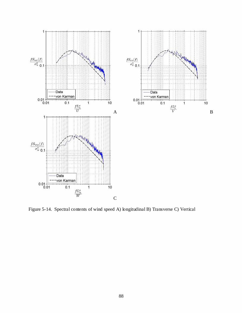
88

A B

C Figure 5-14. Spectral contents of wind speed A) longitudinal B) Transverse C) Vertical

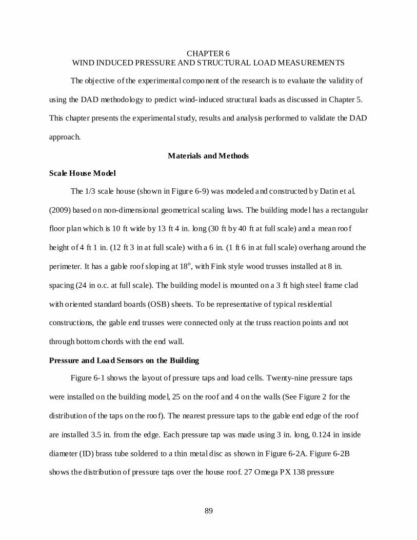
89

CHAPTER 6 WIND INDUCED PRESSURE AND STRUCTURAL LOAD MEASUREMENTS

The objective of the experimental component of the research is to evaluate the validity of

using the DAD methodology to predict wind- induced structural loads as discussed in Chapter 5.

This chapter presents the experimental study, results and analysis performed to validate the DAD

approach.

Materials and Methods

Scale House Model

The 1/3 scale house (shown in Figure 6-9) was modeled and constructed by Datin et al.

(2009) based on non-dimensional geometrical scaling laws. The building model has a rectangular

floor plan which is 10 ft wide by 13 ft 4 in. long (30 ft by 40 ft at full scale) and a mean roo f

height of 4 ft 1 in. (12 ft 3 in at full scale) with a 6 in. (1 ft 6 in at full scale) overhang around the

perimeter. It has a gable roof sloping at 18o, with Fink style wood trusses installed at 8 in.

spacing (24 in o.c. at full scale). The building model is mounted on a 3 ft high steel frame clad

with oriented standard boards (OSB) sheets. To be representative of typical residential

constructions, the gable end trusses were connected only at the truss reaction points and not

through bottom chords with the end wall.

Pressure and Load Sensors on the Building

Figure 6-1 shows the layout of pressure taps and load cells. Twenty-nine pressure taps

were installed on the building model, 25 on the roof and 4 on the walls (See Figure 2 for the

distribution of the taps on the roo f). The nearest pressure taps to the gable end edge of the roof

are installed 3.5 in. from the edge. Each pressure tap was made using 3 in. long, 0.124 in inside

diameter (ID) brass tube soldered to a thin metal disc as shown in Figure 6-2A. Figure 6-2B

shows the distribution of pressure taps over the house roof. 27 Omega PX 138 pressure

90

transducers and 2 Setra model 265 transducers were used to capture pressure distributions on the

roof and walls of the house. The high port of each transducer was connected to the taps via a 6

in. long 3/16 in. ID vinyl clear tube. The internal pressure was measured using a Dwyer 616-20B

transducer. The low ports of the transducers were connected to a single manifold and held at

ambient pressure (see Figure 6-3). The specifications of these transducers are given in Table 6-1.

Pictures of the three different transducers used are shown in Figure 6-4.

Structural reactions on the building were monitored using twenty-one 300 single axes

compression/tension load cells (Futek model LRF 350). Twelve load cells were installed at roof

to wall connections and 9 at the wall-to-foundation connections (see Figure 6-5). The building

was isolated at the instrumented end to capture the total load reactions through this load cell

array.

All these pressure transducers were factory-calibrated. However, a Fluke - 718 1G -

pressure calibrator with serial number of 9916005(shown in Figure 6-6) was used to confirm the

calibration charts. The data acquisition system consisted of a National Instruments (NI)

CompacDAQ chassis (NI cDAQ – 9172) with modules NI 9205 and NI 9219. This data

acquisition system was controlled by Measurement and Automation Explorer and LabView

software version 8.5. Prior to the experiment, the instruments were left overnight to measure

room condition signa ls to check for possible drift effects in their performances.

Test Arrangement

Two 16 ft tall by 34 long wood framed walls were constructed at the exit the UF wind

generator to enclose the test building. The windward face of the 1/3 scale model was placed at

approximately18 ft away from the exit to provide a flow development length of at least four

times the fan diameter (4.5 ft). The house was oriented in three separate directions (0o, 45o and

90o) to the wind flow. Figure 6-8 shows a layout for the experimental set-up. Figures 5-9 shows

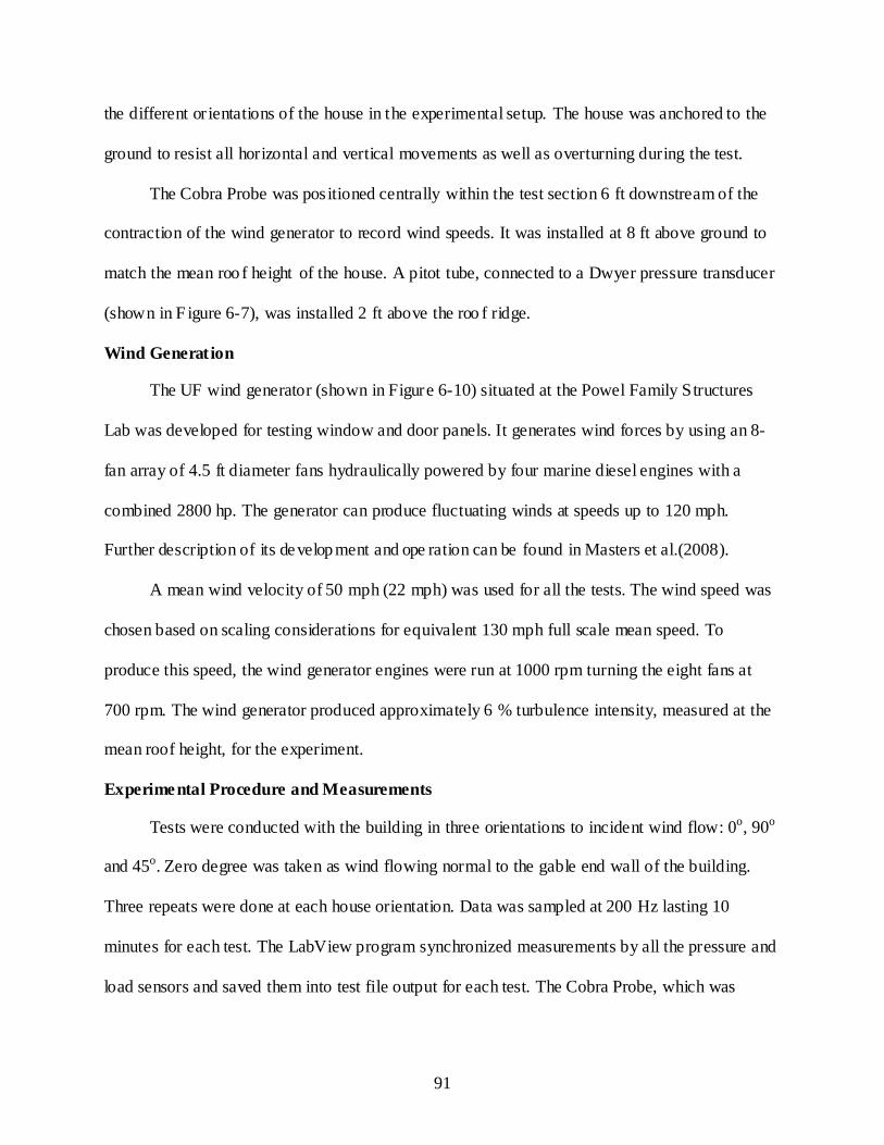
91

the different or ientations of the house in the experimental setup. The house was anchored to the

ground to resist all horizontal and vertical movements as well as overturning during the test.

The Cobra Probe was positioned centrally within the test section 6 ft downstream of the

contraction of the wind generator to record wind speeds. It was installed at 8 ft above ground to

match the mean roo f height of the house. A pitot tube, connected to a Dwyer pressure transducer

(shown in F igure 6-7), was installed 2 ft above the roo f ridge.

Wind Generation

The UF wind generator (shown in Figure 6-10) situated at the Powel Family Structures

Lab was developed for testing window and door panels. It generates wind forces by using an 8-

fan array of 4.5 ft diameter fans hydraulically powered by four marine diesel engines with a

combined 2800 hp. The generator can produce fluctuating winds at speeds up to 120 mph.

Further description of its development and ope ration can be found in Masters et al.(2008).

A mean wind velocity of 50 mph (22 mph) was used for all the tests. The wind speed was

chosen based on scaling considerations for equivalent 130 mph full scale mean speed. To

produce this speed, the wind generator engines were run at 1000 rpm turning the eight fans at

700 rpm. The wind generator produced approximately 6 % turbulence intensity, measured at the

mean roof height, for the experiment.

Experimental Procedure and Measurements

Tests were conducted with the building in three orientations to incident wind flow: 0o, 90o

and 45o. Zero degree was taken as wind flowing normal to the gable end wall of the building.

Three repeats were done at each house orientation. Data was sampled at 200 Hz lasting 10

minutes for each test. The LabView program synchronized measurements by all the pressure and

load sensors and saved them into test file output for each test. The Cobra Probe, which was

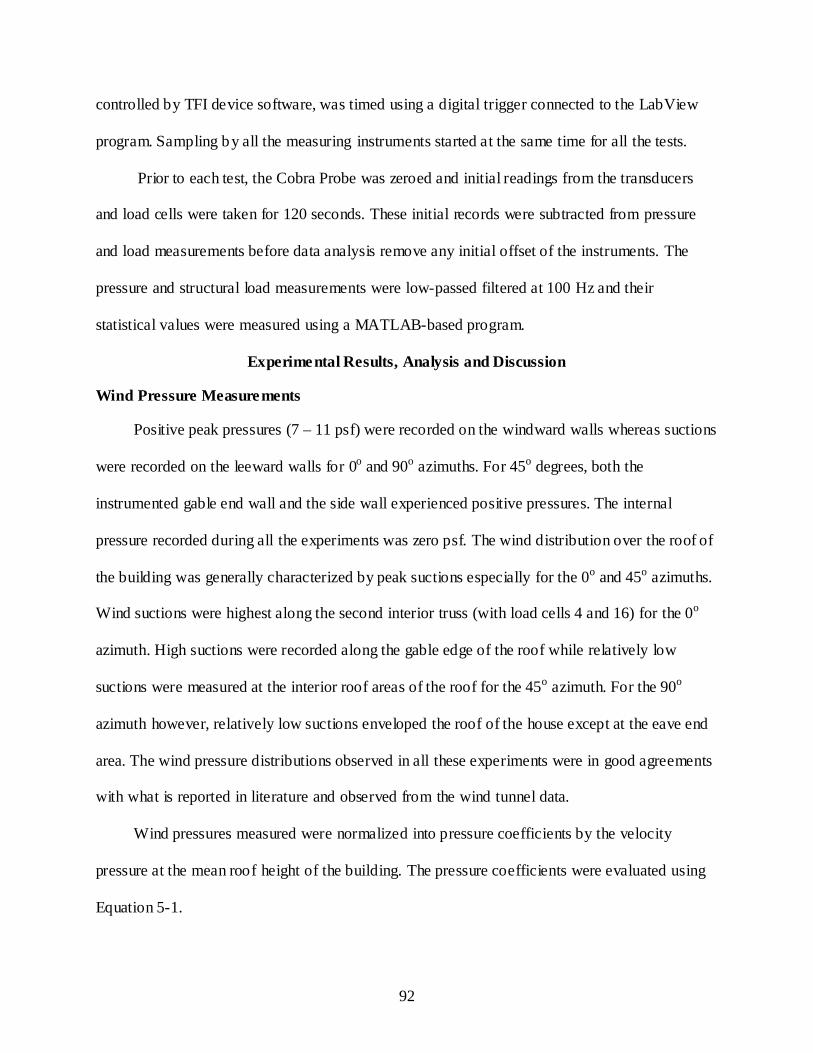
92

controlled by TFI device software, was timed using a digital trigger connected to the LabView

program. Sampling by all the measuring instruments started at the same time for all the tests.

Prior to each test, the Cobra Probe was zeroed and initial readings from the transducers

and load cells were taken for 120 seconds. These initial records were subtracted from pressure

and load measurements before data analysis remove any initial offset of the instruments. The

pressure and structural load measurements were low-passed filtered at 100 Hz and their

statistical values were measured using a MATLAB-based program.

Experimental Results, Analysis and Discussion

Wind Pressure Measurements

Positive peak pressures (7 – 11 psf) were recorded on the windward walls whereas suctions

were recorded on the leeward walls for 0o and 90o azimuths. For 45o degrees, both the

instrumented gable end wall and the side wall experienced positive pressures. The internal

pressure recorded during all the experiments was zero psf. The wind distribution over the roof of

the building was generally characterized by peak suctions especially for the 0o and 45o azimuths.

Wind suctions were highest along the second interior truss (with load cells 4 and 16) for the 0o

azimuth. High suctions were recorded along the gable edge of the roof while relatively low

suctions were measured at the interior roof areas of the roof for the 45o azimuth. For the 90o

azimuth however, relatively low suctions enveloped the roof of the house except at the eave end

area. The wind pressure distributions observed in all these experiments were in good agreements

with what is reported in literature and observed from the wind tunnel data.

Wind pressures measured were normalized into pressure coefficients by the velocity

pressure at the mean roof height of the building. The pressure coefficients were evaluated using

Equation 5-1.

93

2mrh

ii,mrh,p

U2/1

)t(P)t(C

ρ=

(5-1)

where Cp,mrh,i(t) pressure coefficient at pressure tap i at time t, referenced to the mean wind speed

measured at the mean roof height of the building; Pi is the measured wind pressure at tap i; ρ is

the air density; Umrh is mean wind speed (mph) recorded at mean roof height by the Cobra Probe.

Pressure coefficients obtained for the nine test repeats are given in Appendix C. Table 6-2

shows the mean, peak and root mean square (RMS) pressure coefficients averaged from results

of the three datasets for each wind direction. The peak negative and mean pressure coefficients

contour plot results are also shown in Figure 6-11.

Wind-Induced Structural Loads

Measured statistical values of structural loads obtained from each test of the experimental

study are provided in Appendix D. The three sample data obtained for each direction were

augmented. Each augmented time history was then divided into six segments to ob tain six 10-

minute (full scale) samples. Mean, peak and RMS reactions were measured from these segments

and an extreme value analysis (discussed in Chapter 3 and C hapter 4) was used to estimate the

expected positive and negative peak reactions. The Lieblein-BLUE estimators (Lieblein 1974)

used in the analysis of the six samples in each direction are provided in Table 5-3. The mean,

RMS and expected peak values of structural loads measured by the twenty-one load cells are

provided in Table 5-4. These statistical values are average loads from the three datasets for each

wind azimuth. T he locations of the load cells on a 3D drawing of the house are shown in Figure

6-13. Figures 5-14 to 5-16 show the mean, extreme positive and negative structural reactions.

The plots are such that the gable end load cells (15 & 19) are at the center of the roof-to-wall

zone. Load cells on the same truss are mirrored about load cells 15 and 19 on the plots for easy

comparison of measurements.

94

Even though there was no connection between the gable end truss and the gable end wall

except at end supports of the truss, there was considerable load transferred from the gable end

wall to the foundation.

At the 90o azimuth, significantly high reactions were recorded at the gable end wall-to-

foundation load cells than the other load cells. Another unusual observation made for this

direction was that load cell 20 recorded high positive reactions whereas adjacent load cells (19

and 16) recorded relatively high negative reactions. Perhaps, these observations could be

explained by fact that the portion of the building where these load cells were located was not

completely immersed in the wind flow jet (as shown in F igure 5-8) and therefore subjected to

unrealistic wind loads.

For incident 0o azimuth, it is observed that fairly symmetrical loads were recorded at the

roof-to-wall connections on side walls. Also, load cells 4 and 16 recorded highest uplift load (26

psf & 22 psf respectively) on either sidewall suggesting that high suctions experienced along the

second interior truss were mainly transferred through its support. Load cells located at the gable

end measured equally high uplifts as observed in the DAD-based loads of wind tunnel data.

Generally, the structural loads measured at the roof-to-wall connections are highest at the

0o azimuth and lowest at the 90o azimuth. This observation was also made in the case of loads

computed based on wind tunnel data where the highest loads were estimated for the 0o azimuth

and decreased with wind direction increment of 15o.

Structural Load Comparison

The envelope pressures over the house were used to estimate the structural loads being

transferred through roof- to-wall load cell numbers 4, 5 and 15, and foundation load cell number

11. Predictions were made based on the DAD methodology using the experimentally derived

influence coefficients (described in Chapter 4). For comparison with the directly measured

95

structural loads, actual pressure time histories (not pressure coefficients) based on the wind flow

characteristics of the various tests were utilized in the DAD approach as follows:

∑=

××=1i

iijij ))]t(PA)N[()t(R (5-2)

where Rj(t) is load reaction in pounds at the jth connection at time t; (Ni)j is influence coefficient

at the ith grid point for the jth connection; Ai is tributary area of i th grid po int; and Pi(t) is

pressure measured at the ith grid po int at time t.

Figures 6-17 to 6-19 show 1 minute records of measured and evaluated reactions. High

correlations are observed between the reaction time histories of the two records. The highest

correlation coefficient of 0.9 was measured between the records of load cells 15 for the 0o wind

azimuth. Measured correlation coefficients for the records are given in Table 6-5. Even though

the estimated and measured reactions are not in excellent agreement as far as magnitude is

concerned for some the load cells considered, their records show good trends. It is observed that

in almost all the comparisons, the peaks of time histories of the two records seem to be occurring

at the same time. Furthermore, significantly more fluctuating signals were obtained using the

roof pressures relative to the directly measured load cell signa ls. It is worth noting that a similar

observation was made by Zisis & Stathopoulos (2009) in a parallel study. Zisis & Stathopoulos

(2009) attributed this phenomenon to the attenuation effect due to structural and material

damping of the building components thereby lowering the fluctuations in the measured signal.

Peak and mean uplift structural loads measured and estimated for the four load cells are

provided in Table 6-6. Good agreements are observed comparing the mean and peak reaction in

almost all cases. Small discrepancies (lowest is 2%) are seen between the statistical values for

load cell 15 as compared to the others. Generally, the DAD methodology underestimated

structural loads expected to be transferred through the other load cells considered. This may be

96

due to the fact that the effective influence surfaces of these load cells were not completely

covered with pressure taps. Hence, pressure loads which were transferred through these load

cells were not fully captured.

In summary, the DAD methodology adequately predicted the expected loads at roof-to-

wall and wall-to-foundation connections based on realistic wind load paths. The ability to

estimate structural loads on light framed wood structures using t he DAD approach has been

demonstrated in this experimental study.

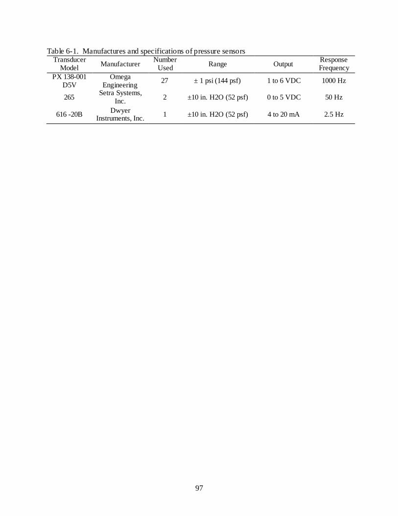
97

Table 6-1. Manufactures and specifications of pressure sensors Transducer

Model Manufacturer Number Used Range Output Response

Frequency PX 138-001

D5V Omega

Engineering 27 ± 1 psi (144 psf) 1 to 6 VDC 1000 Hz

265 Setra Systems, Inc. 2 ±10 in. H2O (52 psf) 0 to 5 VDC 50 Hz

616 -20B Dwyer Instruments, Inc. 1 ±10 in. H2O (52 psf) 4 to 20 mA 2.5 Hz

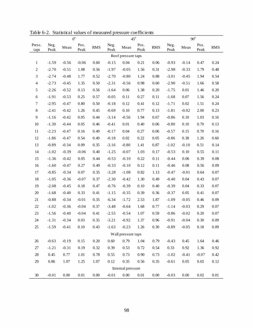
98

Table 6-2. Statistical values of measured pressure coefficients 0o 45o 90o

Press. taps

Neg. Peak Mean Pos.



Peak RMS

Roof pressure taps

1 -1.59 -0.56 -0.06 0.60 -0.15 0.04 0.21 0.06 -0.93 -0.14 0.47 0.24

2 -2.70 -0.51 1.08 0.56 -1.97 -0.05 1.56 0.31 -2.98 -0.33 1.79 0.48

3 -2.74 -0.48 1.77 0.52 -2.70 -0.80 1.24 0.88 -3.01 -0.45 1.94 0.54

4 -2.73 -0.45 1.35 0.50 -2.31 -0.56 0.98 0.60 -2.90 -0.51 1.66 0.58

5 -2.26 -0.52 0.13 0.56 -1.64 0.06 1.38 0.20 -1.75 0.01 1.46 0.20

6 -1.91 -0.53 0.25 0.57 -0.05 0.11 0.27 0.11 -1.68 0.07 1.56 0.24

7 -2.95 -0.47 0.80 0.50 -0.18 0.12 0.41 0.12 -1.71 0.02 1.51 0.24

8 -2.41 -0.42 1.26 0.45 -0.69 0.10 0.77 0.13 -1.81 -0.02 2.00 0.23

9 -1.16 -0.42 0.05 0.44 -3.14 -0.56 1.94 0.67 -0.86 0.10 1.03 0.16

10 -1.30 -0.44 0.05 0.46 -0.41 0.01 0.40 0.06 -0.80 0.10 0.70 0.13

11 -2.23 -0.47 0.16 0.49 -0.17 0.04 0.27 0.06 -0.57 0.15 0.70 0.16

12 -1.86 -0.47 0.54 0.49 -0.18 0.02 0.22 0.05 -0.86 0.38 1.26 0.60

13 -0.89 -0.34 0.09 0.35 -3.16 -0.80 1.41 0.87 -1.02 -0.10 0.51 0.14

14 -1.02 -0.39 -0.06 0.40 -1.25 -0.07 1.03 0.17 -0.53 0.10 0.55 0.11

15 -1.36 -0.42 0.05 0.44 -0.53 -0.10 0.22 0.11 -0.44 0.06 0.39 0.08

16 -1.60 -0.47 0.27 0.49 -0.33 -0.10 0.12 0.11 -0.46 0.08 0.56 0.09

17 -0.85 -0.34 0.07 0.35 -3.28 -1.08 0.82 1.13 -0.47 -0.01 0.64 0.07

18 -1.05 -0.36 -0.07 0.37 -2.30 -0.42 1.30 0.49 -0.40 0.04 0.43 0.07

19 -2.08 -0.45 0.18 0.47 -0.76 -0.39 0.10 0.40 -0.39 0.04 0.33 0.07

20 -1.68 -0.40 0.33 0.41 -1.15 -0.35 0.39 0.36 -0.37 0.05 0.41 0.07

21 -0.88 -0.34 -0.01 0.35 -6.34 -1.72 2.53 1.87 -1.09 -0.05 0.46 0.09

22 -1.02 -0.36 -0.04 0.37 -3.48 -0.64 1.68 0.77 -1.14 -0.03 0.29 0.07

23 -1.56 -0.40 -0.04 0.41 -2.55 -0.54 1.07 0.59 -0.86 -0.02 0.20 0.07

24 -1.31 -0.34 0.03 0.35 -3.21 -0.92 1.37 0.96 -0.91 -0.04 0.30 0.09

25 -1.59 -0.41 0.10 0.43 -1.63 -0.23 1.26 0.30 -0.89 -0.05 0.18 0.09

Wall pressure taps

26 -0.63 -0.19 0.15 0.20 0.60 0.79 1.04 0.79 -0.43 0.45 1.64 0.46

27 -1.21 -0.31 0.19 0.32 0.39 0.53 0.72 0.54 0.33 0.92 1.36 0.92

28 0.45 0.77 1.01 0.78 0.55 0.73 0.90 0.73 -1.02 -0.41 -0.07 0.42

29 0.86 1.07 1.25 1.07 0.12 0.35 0.56 0.35 -0.61 0.05 0.65 0.12

Internal pressure

30 -0.01 0.00 0.01 0.00 -0.01 0.00 0.01 0.00 -0.03 0.00 0.02 0.01

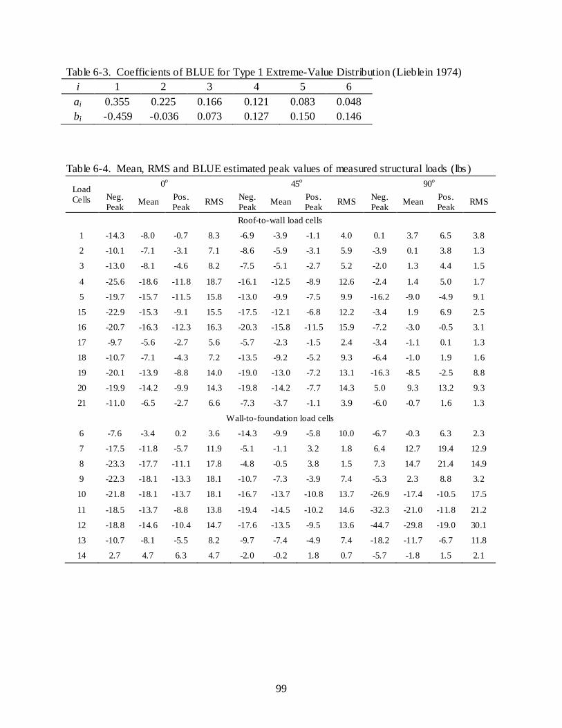
99

Table 6-3. Coefficients of BLUE for Type 1 Extreme-Value Distribution (Lieblein 1974) i 1 2 3 4 5 6 ai 0.355 0.225 0.166 0.121 0.083 0.048 bi -0.459 -0.036 0.073 0.127 0.150 0.146

Table 6-4. Mean, RMS and BLUE estimated peak values of measured structural loads (lbs )

Load Cells

0o 45o 90o Neg. Peak Mean Pos.



Peak RMS

Roof-to-wall load cells

1 -14.3 -8.0 -0.7 8.3 -6.9 -3.9 -1.1 4.0 0.1 3.7 6.5 3.8

2 -10.1 -7.1 -3.1 7.1 -8.6 -5.9 -3.1 5.9 -3.9 0.1 3.8 1.3

3 -13.0 -8.1 -4.6 8.2 -7.5 -5.1 -2.7 5.2 -2.0 1.3 4.4 1.5

4 -25.6 -18.6 -11.8 18.7 -16.1 -12.5 -8.9 12.6 -2.4 1.4 5.0 1.7

5 -19.7 -15.7 -11.5 15.8 -13.0 -9.9 -7.5 9.9 -16.2 -9.0 -4.9 9.1

15 -22.9 -15.3 -9.1 15.5 -17.5 -12.1 -6.8 12.2 -3.4 1.9 6.9 2.5

16 -20.7 -16.3 -12.3 16.3 -20.3 -15.8 -11.5 15.9 -7.2 -3.0 -0.5 3.1

17 -9.7 -5.6 -2.7 5.6 -5.7 -2.3 -1.5 2.4 -3.4 -1.1 0.1 1.3

18 -10.7 -7.1 -4.3 7.2 -13.5 -9.2 -5.2 9.3 -6.4 -1.0 1.9 1.6

19 -20.1 -13.9 -8.8 14.0 -19.0 -13.0 -7.2 13.1 -16.3 -8.5 -2.5 8.8

20 -19.9 -14.2 -9.9 14.3 -19.8 -14.2 -7.7 14.3 5.0 9.3 13.2 9.3

21 -11.0 -6.5 -2.7 6.6 -7.3 -3.7 -1.1 3.9 -6.0 -0.7 1.6 1.3

Wall-to-foundation load cells

6 -7.6 -3.4 0.2 3.6 -14.3 -9.9 -5.8 10.0 -6.7 -0.3 6.3 2.3

7 -17.5 -11.8 -5.7 11.9 -5.1 -1.1 3.2 1.8 6.4 12.7 19.4 12.9

8 -23.3 -17.7 -11.1 17.8 -4.8 -0.5 3.8 1.5 7.3 14.7 21.4 14.9

9 -22.3 -18.1 -13.3 18.1 -10.7 -7.3 -3.9 7.4 -5.3 2.3 8.8 3.2

10 -21.8 -18.1 -13.7 18.1 -16.7 -13.7 -10.8 13.7 -26.9 -17.4 -10.5 17.5

11 -18.5 -13.7 -8.8 13.8 -19.4 -14.5 -10.2 14.6 -32.3 -21.0 -11.8 21.2

12 -18.8 -14.6 -10.4 14.7 -17.6 -13.5 -9.5 13.6 -44.7 -29.8 -19.0 30.1

13 -10.7 -8.1 -5.5 8.2 -9.7 -7.4 -4.9 7.4 -18.2 -11.7 -6.7 11.8

14 2.7 4.7 6.3 4.7 -2.0 -0.2 1.8 0.7 -5.7 -1.8 1.5 2.1

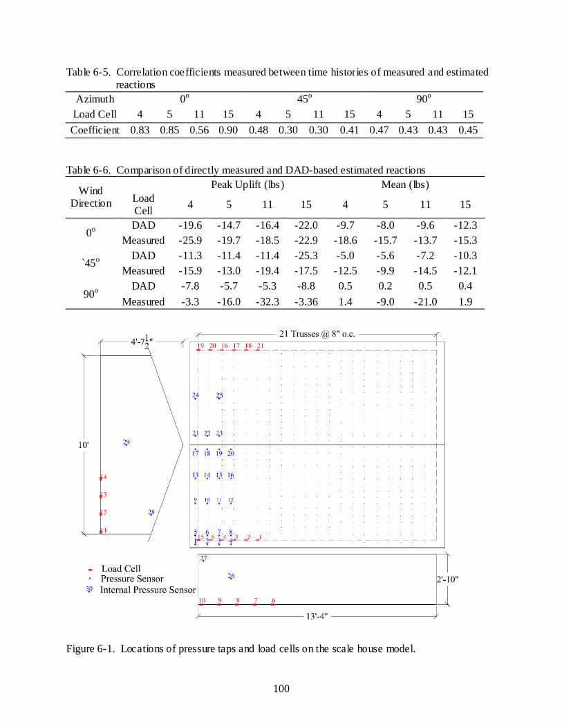
100

Table 6-5. Correlation coefficients measured between time histories of measured and estimated reactions

Azimuth 0o 45o 90o Load Cell 4 5 11 15 4 5 11 15 4 5 11 15 Coefficient 0.83 0.85 0.56 0.90 0.48 0.30 0.30 0.41 0.47 0.43 0.43 0.45

Table 6-6. Comparison of directly measured and DAD-based estimated reactions

Wind Direction

Peak Uplift (lbs) Mean (lbs) Load Cell 4 5 11 15 4 5 11 15

0o DAD -19.6 -14.7 -16.4 -22.0 -9.7 -8.0 -9.6 -12.3

Measured -25.9 -19.7 -18.5 -22.9 -18.6 -15.7 -13.7 -15.3

`45o DAD -11.3 -11.4 -11.4 -25.3 -5.0 -5.6 -7.2 -10.3

Measured -15.9 -13.0 -19.4 -17.5 -12.5 -9.9 -14.5 -12.1

90o DAD -7.8 -5.7 -5.3 -8.8 0.5 0.2 0.5 0.4

Measured -3.3 -16.0 -32.3 -3.36 1.4 -9.0 -21.0 1.9

Figure 6-1. Locations of pressure taps and load cells on the scale house model.

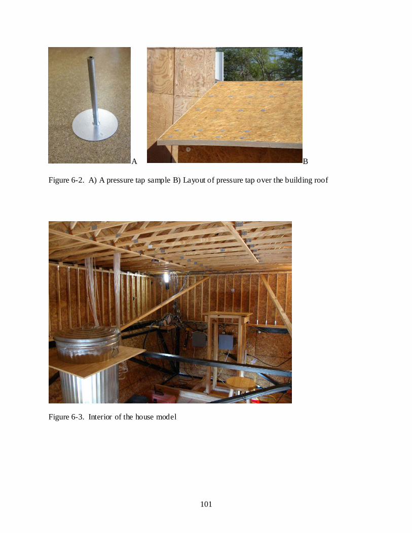
101

A B Figure 6-2. A) A pressure tap sample B) Layout of pressure tap over the building roof

Figure 6-3. Interior of the house model

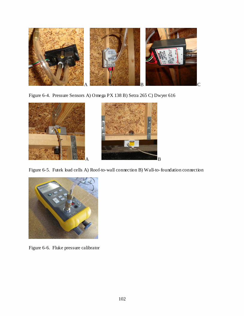
102

A B C Figure 6-4. Pressure Sensors A) Omega PX 138 B) Setra 265 C) Dwyer 616

A B Figure 6-5. Futek load cells A) Roof-to-wall connection B) Wall-to-foundation connection

Figure 6-6. Fluke pressure calibrator

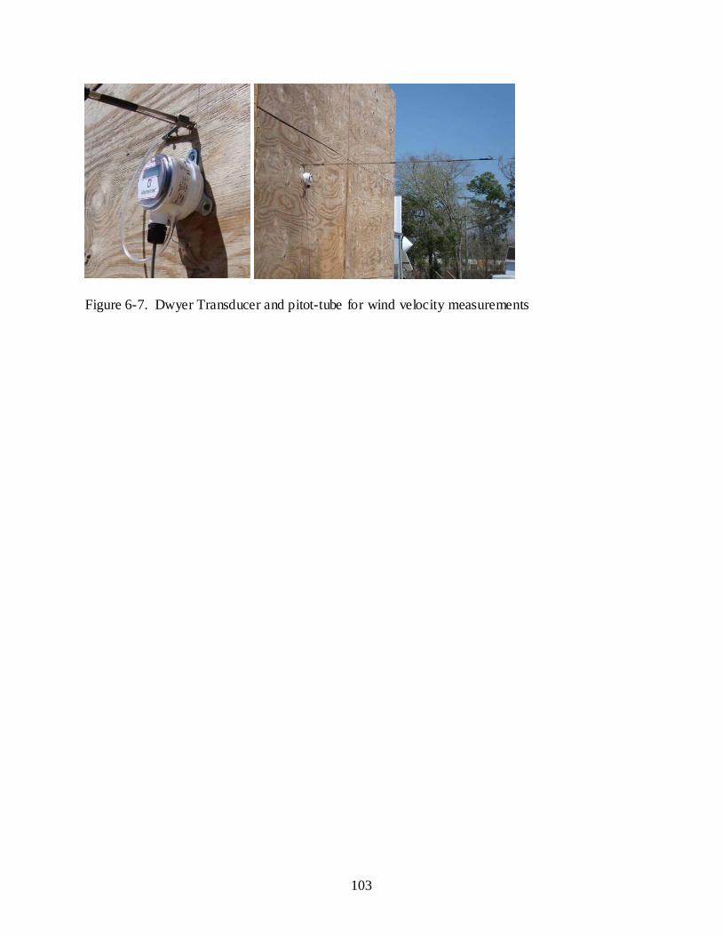
103

Figure 6-7. Dwyer Transducer and pitot-tube for wind velocity measurements

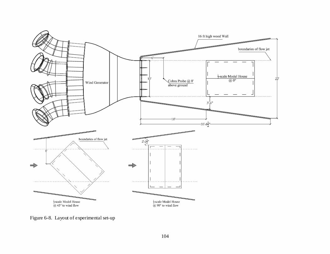
104

Figure 6-8. Layout of experimental set-up

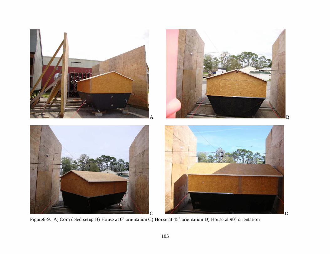
105

A B

C D Figure6-9. A) Completed setup B) House at 0o or ientation C) House at 45o or ientation D) House at 90o orientation

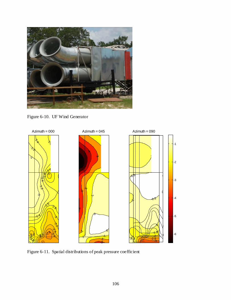
106

Figure 6-10. UF Wind Generator

-2.6-2.4

-2.2

-2.2

-2

-2

-1.8

-1.6

-1.6

-1.6

-1.4-1.4

-1.4

-1.2

-1.2

-1

-1

-1.8

-2-2.8

-1.8

-2

-2.2

Azimuth = 000

-6-5

-4

-4

-3

-3

-3

-2

-2

-2

-2-1

-1

-1

0

0

-1

Azimuth = 045

-3-2.5

-2-1.5

-1.5

-1

-1

-1

-0.5

-0.5

-1

Azimuth = 090

64

2

2

8

6

6

-6

-5

-4

-3

-2

-1

Figure 6-11. Spatial distributions of peak pressure coefficient

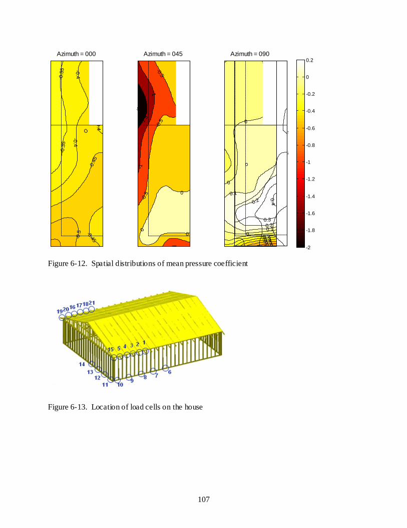
107

-0.5

-0.4

5

-0.4-0.4

-0.3

5-0

.35

-0.45-0.4

Azimuth = 000

-2

-1.5

-1

-1

-0.5

-0.5

-0.5

0

0

0

0

Azimuth = 045

-0.6-0.5-0.4-0.3-0.2

-0.1

0

0

0

0.1

0.10.2

0.2

0.3

0.4

Azimuth = 090

5

4

-2

-1.8

-1.6

-1.4

-1.2

-1

-0.8

-0.6

-0.4

-0.2

0

0.2

Figure 6-12. Spatial distributions of mean pressure coefficient

Figure 6-13. Location of load cells on the house

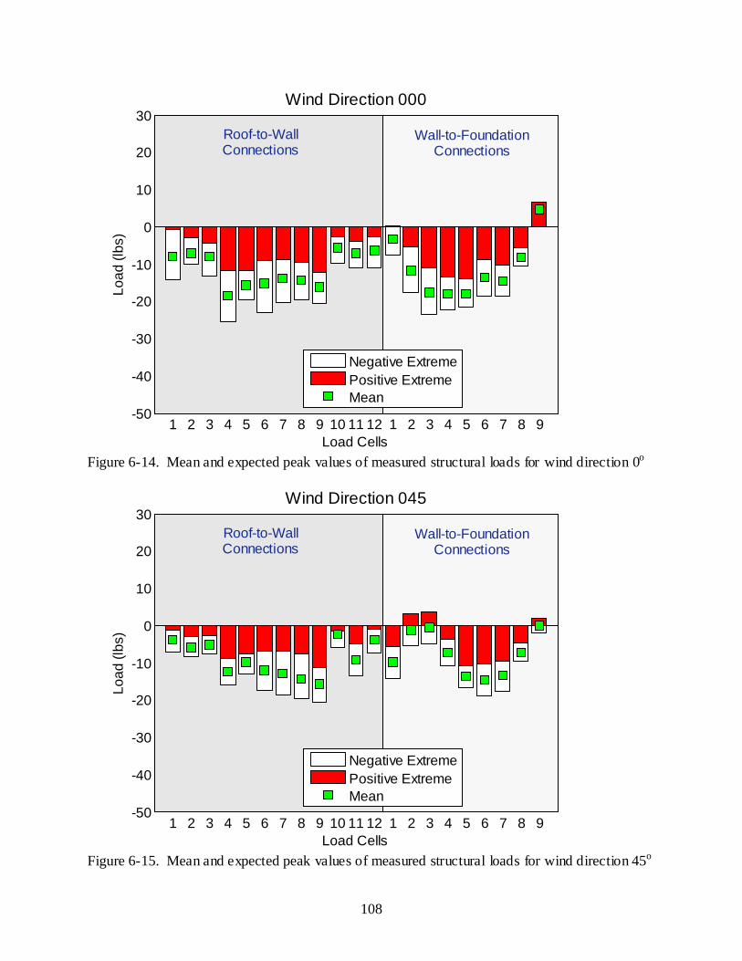
108

1 2 3 4 5 6 7 8 9 10 11 12 1 2 3 4 5 6 7 8 9-50

-40

-30

-20

-10

0

10

20

30Lo

ad (l

bs)

Load Cells

Wind Direction 000




Figure 6-14. Mean and expected peak values of measured structural loads for wind direction 0o

1 2 3 4 5 6 7 8 9 10 11 12 1 2 3 4 5 6 7 8 9-50

-40

-30

-20

-10

0

10

20

30

Load

(lbs

)

Load Cells

Wind Direction 045





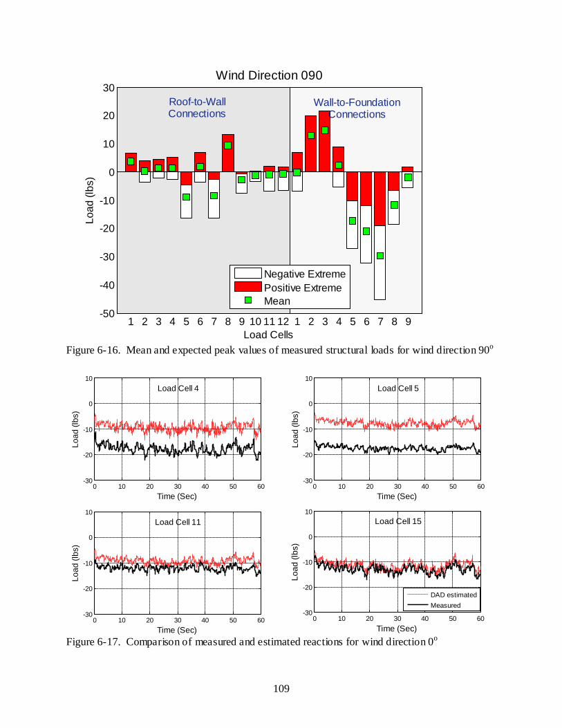
109

1 2 3 4 5 6 7 8 9 10 11 12 1 2 3 4 5 6 7 8 9-50

-40

-30

-20

-10

0

10

20

30Lo

ad (l

bs)

Load Cells

Wind Direction 090





0 10 20 30 40 50 60-30

-20

-10

0

10

Time (Sec)

Load

(lbs

)

Load Cell 4

0 10 20 30 40 50 60

-30

-20

-10

0

10

Time (Sec)

Load

(lbs

)

Load Cell 5

0 10 20 30 40 50 60-30

-20

-10

0

10

Time (Sec)

Load

(lbs

)

Load Cell 11

0 10 20 30 40 50 60

-30

-20

-10

0

10

Time (Sec)

Load

(lbs

)

DAD estimatedMeasured

Load Cell 15

Figure 6-17. Comparison of measured and estimated reactions for wind direction 0o

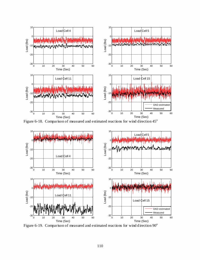
110

0 10 20 30 40 50 60-30

-20

-10

0

10

Time (Sec)

Load

(lbs

)Load Cell 4

0 10 20 30 40 50 60

-30

-20

-10

0

10

Time (Sec)

Load

(lbs

)

Load Cell 5

0 10 20 30 40 50 60-30

-20

-10

0

10

Time (Sec)

Load

(lbs

)

Load Cell 11

0 10 20 30 40 50 60

-30

-20

-10

0

10

Time (Sec)

Load

(lbs

)


Load Cell 15

Figure 6-18. Comparison of measured and estimated reactions for wind direction 45o

0 10 20 30 40 50 60-30

-20

-10

0

10

Time (Sec)

Load

(lbs

)

Load Cell 4

0 10 20 30 40 50 60

-30

-20

-10

0

10

Time (Sec)

Load

(lbs

)

Load Cell 5

0 10 20 30 40 50 60-30

-20

-10

0

10

Time (Sec)

Load

(lbs

)

Load Cell 11

0 10 20 30 40 50 60

-30

-20

-10

0

10

Time (Sec)

Load

(lbs

)


Load Cell 15

Figure 6-19. Comparison of measured and estimated reactions for wind d irection 90o

111

CHAPTER 7 CONCLUSION AND RECOMMENDATIONS

This chapter provides a summary of work undertaken and key findings made. Significant

conclus ions which can be drawn from the study as well as recommenda tions for future research

in this study area are discussed.

Summary

Light framed wood structures (LFWS) are by far the largest contributor to monetary losses

associated hurricane damages. Inadequate load transfer mechanism provided in wood

constructions account significantly to structural failures of such buildings. The need for studies

to provide better understanding of wind load paths on LFWS buildings cannot be overemphasize.

This research was aimed at estimating wind- induced s tructural loads transferred through

roof-to-wall and wall- to-foundation connections on LFWS. The estimations were based on

Database-Assisted Design (DAD) methodology, developed by the National Institute of Standards

and Technology (NIST). This methodology, which utilizes large databases of aerodynamic

pressures and climatological information, has been used by other researchers to predict structural

responses due to wind forces on steel portal frame buildings. This current study, apart from

extending the application of the DAD approach to LFWS, also demonstrates the validity of this

methodo logy to adequately evaluate structural reactions on LFWS.

The project was accomplished in two phases: a hybridized analytical approach and an

experimental approach. In the former, spatially distributed pressure coefficients were derived

from wind tunnel data for a 1/50 scale model house. These pressure coefficients (time histories)

were combined with structural influence coefficients (developed on a 1/3 scale model wood

house) through computer-based analysis to generate structural reactions. Peak uplift reactions

were estimated from a Lieblein BLUE-fitted distribution of the measured peak reactions. These

112

were then compared to wind design loads based on ASCE-7 provisions for both Main Wind

Force Resisting Systems (MWFRS) and Components and Cladding (C&C). It was realized that

using MWFRS pressures underestimated the reactions by up to 32% while C&C provisions

resulted in highly conservative estimates (up to 60% overestimation).

In the experimental study, the 1/3-scale wood house model was instrumented with pressure

and load sensors. The house was subjected to wind forces while load and pressure measurements

were simultaneously taken. Based on the DAD approach, structural reactions were estimated

using measured roof pressures and results were compared to directly-measured structural loads.

Even though significantly fluctuating reaction records were obtained using the DAD in

comparison to the directly measured reaction records, the two quantities were highly correlated.

Again, good agreements were found comparing mean and peak values of the estimated and

measured reactions.

Conclusions

The conclusions of this study can be summarized as follows:

1. Local peak pressure coefficients derived from wind tunnel analysis are considerably higher, in most cases, than ASCE 7-05 component and cladding external pressure coefficients. However, an excellent agreement is observed be tween the wind tunnel area-averaged pressure coefficients and the ASCE 7 standard provisions.

2. ASCE 7-05 MWFRS provisions produced lower peak reactions ( average of 21% lower) than predictions based on DAD methodology while predictions based on ASCE 7-05 components and cladding were generally higher.(average of 33 % higher) than DAD-based reactions.

3. Despite limited match of the wind generated in the experiment to realistic wind flows, overall the roo f pressure distributions on the 1/3-scale house were reasonably matched to the wind tunnel pressure spatial distributions in the literature.

4. The structural reaction time history obtained using the DAD method had greater dynamic content than the time history of directly measured structural reactions. Despite this fact there was still good a greement between the peak values and the mean values of DAD results and the measured reactions.

113

5. DAD-based reactions were highly correlated with directly measured structural reactions.

6. Both the analytical and experimental components of this study confirmed that maximum uplifts loads are transferred through the gable end suppor ts.

7. Lastly, a wider spread of load sharing through wall- to-foundation connection was observed in both analytical and experimental studies. This may be due to diaphragm (deep beam) actions of the building walls.

Finally, the study has not just extended the app lication of DAD methodo logy to LFWS but

has evaluated its validity to adequately evaluate structural reactions on LFWS through an

experimental study.

Recommendation

Notwithstanding the significant findings reported in this study and its possible influence on

design practices for LFWS, further research is needed in order to fully comprehend wind load

paths in LFWS. Recommendations for future research in this discipline are discussed below.

1. The study house is a simple rectangular gable roof structure. Most typical residential structures have complex shapes which may result in different pressure distributions on houses and subsequently different wind load pa ths. I t is recommended that studies are done on LFWS with complex building shapes and different configurations.

2. In future experimental studies, load cells should be installed around the whole perimeter of the 1/3-scale building at roof-to-wall and wall-to-foundation interfaces. This will ensure that wind load paths are not unduly affected by the stiffness of the load cells.

3. Also, the entire roof of the house should be equipped with pressure sensors so that the DAD methodo logy could be validated at all critical connections.

4. A better boundary layer condition should be created for future experiments so that comparison can be made between field and wind tunnel measurements.

5. Reliability studies should be carried out to quantify the uncertainty parameters for load estimations on LFWS based on DAD approach.

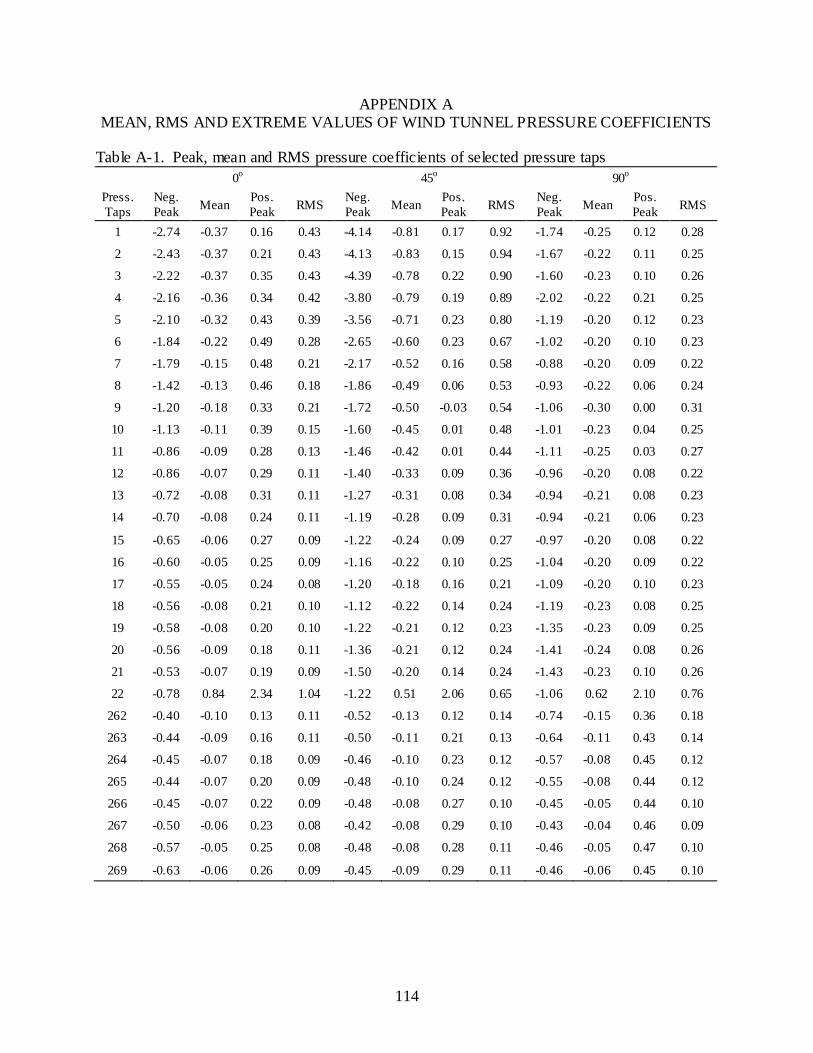
114

APPENDIX A MEAN, RMS AND EXTREME VALUES OF WIND TUNNEL PRESSURE COEFFICIENTS

Table A-1. Peak, mean and RMS pressure coefficients of selected pressure taps 0o 45o 90o

Press. Taps

Neg. Peak Mean Pos.



Peak RMS

1 -2.74 -0.37 0.16 0.43 -4.14 -0.81 0.17 0.92 -1.74 -0.25 0.12 0.28

2 -2.43 -0.37 0.21 0.43 -4.13 -0.83 0.15 0.94 -1.67 -0.22 0.11 0.25

3 -2.22 -0.37 0.35 0.43 -4.39 -0.78 0.22 0.90 -1.60 -0.23 0.10 0.26

4 -2.16 -0.36 0.34 0.42 -3.80 -0.79 0.19 0.89 -2.02 -0.22 0.21 0.25

5 -2.10 -0.32 0.43 0.39 -3.56 -0.71 0.23 0.80 -1.19 -0.20 0.12 0.23

6 -1.84 -0.22 0.49 0.28 -2.65 -0.60 0.23 0.67 -1.02 -0.20 0.10 0.23

7 -1.79 -0.15 0.48 0.21 -2.17 -0.52 0.16 0.58 -0.88 -0.20 0.09 0.22

8 -1.42 -0.13 0.46 0.18 -1.86 -0.49 0.06 0.53 -0.93 -0.22 0.06 0.24

9 -1.20 -0.18 0.33 0.21 -1.72 -0.50 -0.03 0.54 -1.06 -0.30 0.00 0.31

10 -1.13 -0.11 0.39 0.15 -1.60 -0.45 0.01 0.48 -1.01 -0.23 0.04 0.25

11 -0.86 -0.09 0.28 0.13 -1.46 -0.42 0.01 0.44 -1.11 -0.25 0.03 0.27

12 -0.86 -0.07 0.29 0.11 -1.40 -0.33 0.09 0.36 -0.96 -0.20 0.08 0.22

13 -0.72 -0.08 0.31 0.11 -1.27 -0.31 0.08 0.34 -0.94 -0.21 0.08 0.23

14 -0.70 -0.08 0.24 0.11 -1.19 -0.28 0.09 0.31 -0.94 -0.21 0.06 0.23

15 -0.65 -0.06 0.27 0.09 -1.22 -0.24 0.09 0.27 -0.97 -0.20 0.08 0.22

16 -0.60 -0.05 0.25 0.09 -1.16 -0.22 0.10 0.25 -1.04 -0.20 0.09 0.22

17 -0.55 -0.05 0.24 0.08 -1.20 -0.18 0.16 0.21 -1.09 -0.20 0.10 0.23

18 -0.56 -0.08 0.21 0.10 -1.12 -0.22 0.14 0.24 -1.19 -0.23 0.08 0.25

19 -0.58 -0.08 0.20 0.10 -1.22 -0.21 0.12 0.23 -1.35 -0.23 0.09 0.25

20 -0.56 -0.09 0.18 0.11 -1.36 -0.21 0.12 0.24 -1.41 -0.24 0.08 0.26

21 -0.53 -0.07 0.19 0.09 -1.50 -0.20 0.14 0.24 -1.43 -0.23 0.10 0.26

22 -0.78 0.84 2.34 1.04 -1.22 0.51 2.06 0.65 -1.06 0.62 2.10 0.76

262 -0.40 -0.10 0.13 0.11 -0.52 -0.13 0.12 0.14 -0.74 -0.15 0.36 0.18

263 -0.44 -0.09 0.16 0.11 -0.50 -0.11 0.21 0.13 -0.64 -0.11 0.43 0.14

264 -0.45 -0.07 0.18 0.09 -0.46 -0.10 0.23 0.12 -0.57 -0.08 0.45 0.12

265 -0.44 -0.07 0.20 0.09 -0.48 -0.10 0.24 0.12 -0.55 -0.08 0.44 0.12

266 -0.45 -0.07 0.22 0.09 -0.48 -0.08 0.27 0.10 -0.45 -0.05 0.44 0.10

267 -0.50 -0.06 0.23 0.08 -0.42 -0.08 0.29 0.10 -0.43 -0.04 0.46 0.09

268 -0.57 -0.05 0.25 0.08 -0.48 -0.08 0.28 0.11 -0.46 -0.05 0.47 0.10

269 -0.63 -0.06 0.26 0.09 -0.45 -0.09 0.29 0.11 -0.46 -0.06 0.45 0.10

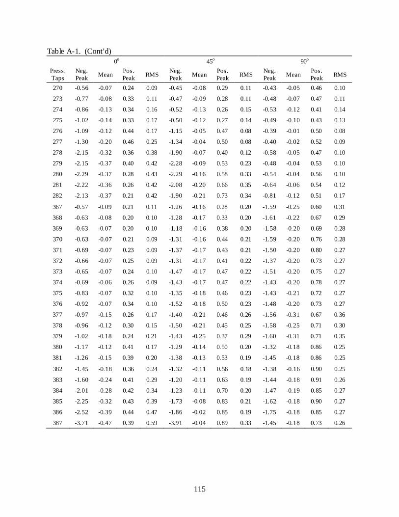
115

Table A-1. (Cont’d) 0o 45o 90o

Press. Taps

Neg. Peak Mean Pos.



Peak RMS

270 -0.56 -0.07 0.24 0.09 -0.45 -0.08 0.29 0.11 -0.43 -0.05 0.46 0.10

273 -0.77 -0.08 0.33 0.11 -0.47 -0.09 0.28 0.11 -0.48 -0.07 0.47 0.11

274 -0.86 -0.13 0.34 0.16 -0.52 -0.13 0.26 0.15 -0.53 -0.12 0.41 0.14

275 -1.02 -0.14 0.33 0.17 -0.50 -0.12 0.27 0.14 -0.49 -0.10 0.43 0.13

276 -1.09 -0.12 0.44 0.17 -1.15 -0.05 0.47 0.08 -0.39 -0.01 0.50 0.08

277 -1.30 -0.20 0.46 0.25 -1.34 -0.04 0.50 0.08 -0.40 -0.02 0.52 0.09

278 -2.15 -0.32 0.36 0.38 -1.90 -0.07 0.40 0.12 -0.58 -0.05 0.47 0.10

279 -2.15 -0.37 0.40 0.42 -2.28 -0.09 0.53 0.23 -0.48 -0.04 0.53 0.10

280 -2.29 -0.37 0.28 0.43 -2.29 -0.16 0.58 0.33 -0.54 -0.04 0.56 0.10

281 -2.22 -0.36 0.26 0.42 -2.08 -0.20 0.66 0.35 -0.64 -0.06 0.54 0.12

282 -2.13 -0.37 0.21 0.42 -1.90 -0.21 0.73 0.34 -0.81 -0.12 0.51 0.17

367 -0.57 -0.09 0.21 0.11 -1.26 -0.16 0.28 0.20 -1.59 -0.25 0.60 0.31

368 -0.63 -0.08 0.20 0.10 -1.28 -0.17 0.33 0.20 -1.61 -0.22 0.67 0.29

369 -0.63 -0.07 0.20 0.10 -1.18 -0.16 0.38 0.20 -1.58 -0.20 0.69 0.28

370 -0.63 -0.07 0.21 0.09 -1.31 -0.16 0.44 0.21 -1.59 -0.20 0.76 0.28

371 -0.69 -0.07 0.23 0.09 -1.37 -0.17 0.43 0.21 -1.50 -0.20 0.80 0.27

372 -0.66 -0.07 0.25 0.09 -1.31 -0.17 0.41 0.22 -1.37 -0.20 0.73 0.27

373 -0.65 -0.07 0.24 0.10 -1.47 -0.17 0.47 0.22 -1.51 -0.20 0.75 0.27

374 -0.69 -0.06 0.26 0.09 -1.43 -0.17 0.47 0.22 -1.43 -0.20 0.78 0.27

375 -0.83 -0.07 0.32 0.10 -1.35 -0.18 0.46 0.23 -1.43 -0.21 0.72 0.27

376 -0.92 -0.07 0.34 0.10 -1.52 -0.18 0.50 0.23 -1.48 -0.20 0.73 0.27

377 -0.97 -0.15 0.26 0.17 -1.40 -0.21 0.46 0.26 -1.56 -0.31 0.67 0.36

378 -0.96 -0.12 0.30 0.15 -1.50 -0.21 0.45 0.25 -1.58 -0.25 0.71 0.30

379 -1.02 -0.18 0.24 0.21 -1.43 -0.25 0.37 0.29 -1.60 -0.31 0.71 0.35

380 -1.17 -0.12 0.41 0.17 -1.29 -0.14 0.50 0.20 -1.32 -0.18 0.86 0.25

381 -1.26 -0.15 0.39 0.20 -1.38 -0.13 0.53 0.19 -1.45 -0.18 0.86 0.25

382 -1.45 -0.18 0.36 0.24 -1.32 -0.11 0.56 0.18 -1.38 -0.16 0.90 0.25

383 -1.60 -0.24 0.41 0.29 -1.20 -0.11 0.63 0.19 -1.44 -0.18 0.91 0.26

384 -2.01 -0.28 0.42 0.34 -1.23 -0.11 0.70 0.20 -1.47 -0.19 0.85 0.27

385 -2.25 -0.32 0.43 0.39 -1.73 -0.08 0.83 0.21 -1.62 -0.18 0.90 0.27

386 -2.52 -0.39 0.44 0.47 -1.86 -0.02 0.85 0.19 -1.75 -0.18 0.85 0.27

387 -3.71 -0.47 0.39 0.59 -3.91 -0.04 0.89 0.33 -1.45 -0.18 0.73 0.26

116

APPENDIX B MEASURED STATISTICAL VALUES OF VERTICAL REACTIONS DERIVED FROM

WIND TUNNEL DATA

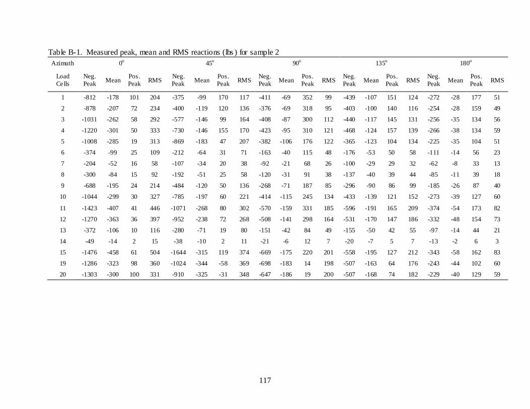
117

Table B-1. Measured peak, mean and RMS reactions (lbs ) for sample 2 Azimuth 0o 45o 90o 135o 180o

Load Cells

Neg. Peak Mean Pos.





Peak RMS

1 -812 -178 101 204 -375 -99 170 117 -411 -69 352 99 -439 -107 151 124 -272 -28 177 51

2 -878 -207 72 234 -400 -119 120 136 -376 -69 318 95 -403 -100 140 116 -254 -28 159 49

3 -1031 -262 58 292 -577 -146 99 164 -408 -87 300 112 -440 -117 145 131 -256 -35 134 56

4 -1220 -301 50 333 -730 -146 155 170 -423 -95 310 121 -468 -124 157 139 -266 -38 134 59

5 -1008 -285 19 313 -869 -183 47 207 -382 -106 176 122 -365 -123 104 134 -225 -35 104 51

6 -374 -99 25 109 -212 -64 31 71 -163 -40 115 48 -176 -53 50 58 -111 -14 56 23

7 -204 -52 16 58 -107 -34 20 38 -92 -21 68 26 -100 -29 29 32 -62 -8 33 13

8 -300 -84 15 92 -192 -51 25 58 -120 -31 91 38 -137 -40 39 44 -85 -11 39 18

9 -688 -195 24 214 -484 -120 50 136 -268 -71 187 85 -296 -90 86 99 -185 -26 87 40

10 -1044 -299 30 327 -785 -197 60 221 -414 -115 245 134 -433 -139 121 152 -273 -39 127 60

11 -1423 -407 41 446 -1071 -268 80 302 -570 -159 331 185 -596 -191 165 209 -374 -54 173 82

12 -1270 -363 36 397 -952 -238 72 268 -508 -141 298 164 -531 -170 147 186 -332 -48 154 73

13 -372 -106 10 116 -280 -71 19 80 -151 -42 84 49 -155 -50 42 55 -97 -14 44 21

14 -49 -14 2 15 -38 -10 2 11 -21 -6 12 7 -20 -7 5 7 -13 -2 6 3

15 -1476 -458 61 504 -1644 -315 119 374 -669 -175 220 201 -558 -195 127 212 -343 -58 162 83

19 -1286 -323 98 360 -1024 -344 -58 369 -698 -183 14 198 -507 -163 64 176 -243 -44 102 60

20 -1303 -300 100 331 -910 -325 -31 348 -647 -186 19 200 -507 -168 74 182 -229 -40 129 59

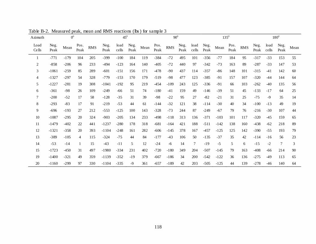
118


Load Cells

Neg. Peak Mean Pos.

Peak RMS Neg. Peak

load cells

Neg. Peak Mean Pos.

Peak RMS Neg. Peak

load cells

Neg. Peak Mean Pos.

Peak RMS Neg. Peak

load cells

Neg. Peak Mean

1 -771 -179 104 205 -399 -100 184 119 -384 -72 495 101 -356 -77 184 95 -317 -33 153 55

2 -858 -206 96 233 -494 -123 164 140 -405 -72 440 97 -342 -73 163 89 -287 -33 147 53

3 -1061 -259 85 289 -601 -151 156 171 -478 -90 437 114 -357 -86 148 101 -315 -41 142 60

4 -1327 -297 54 328 -779 -153 170 179 -519 -98 477 123 -385 -91 157 107 -320 -44 144 64

5 -1227 -281 19 308 -1041 -192 95 219 -454 -109 243 125 -336 -91 66 103 -262 -40 135 56

6 -361 -98 26 109 -249 -66 51 74 -180 -41 159 49 -146 -39 51 45 -133 -17 64 25

7 -200 -52 17 58 -128 -35 31 39 -98 -22 95 27 -82 -21 31 25 -75 -9 35 14

8 -293 -83 17 91 -219 -53 44 61 -144 -32 121 38 -114 -30 40 34 -100 -13 49 19

9 -696 -193 27 212 -553 -125 100 143 -328 -73 244 87 -249 -67 79 76 -216 -30 107 44

10 -1087 -295 20 324 -903 -205 134 233 -498 -118 313 136 -371 -103 101 117 -320 -45 159 65

11 -1479 -402 22 441 -1237 -280 178 318 -681 -164 421 188 -511 -142 138 160 -438 -62 218 89

12 -1321 -358 20 393 -1104 -248 161 282 -606 -145 378 167 -457 -125 125 142 -390 -55 193 79

13 -389 -105 4 115 -324 -75 44 84 -177 -43 106 50 -135 -37 35 42 -114 -16 56 23

14 -53 -14 1 15 -43 -11 5 12 -24 -6 14 7 -19 -5 5 6 -15 -2 7 3

15 -1723 -450 31 497 -1980 -334 231 402 -720 -180 349 204 -507 -145 79 163 -408 -66 214 90

19 -1400 -321 49 359 -1139 -352 -19 379 -667 -186 34 200 -542 -122 36 136 -275 -49 113 65

20 -1160 -299 97 330 -1104 -335 -9 361 -657 -189 42 203 -505 -125 44 139 -278 -46 140 64

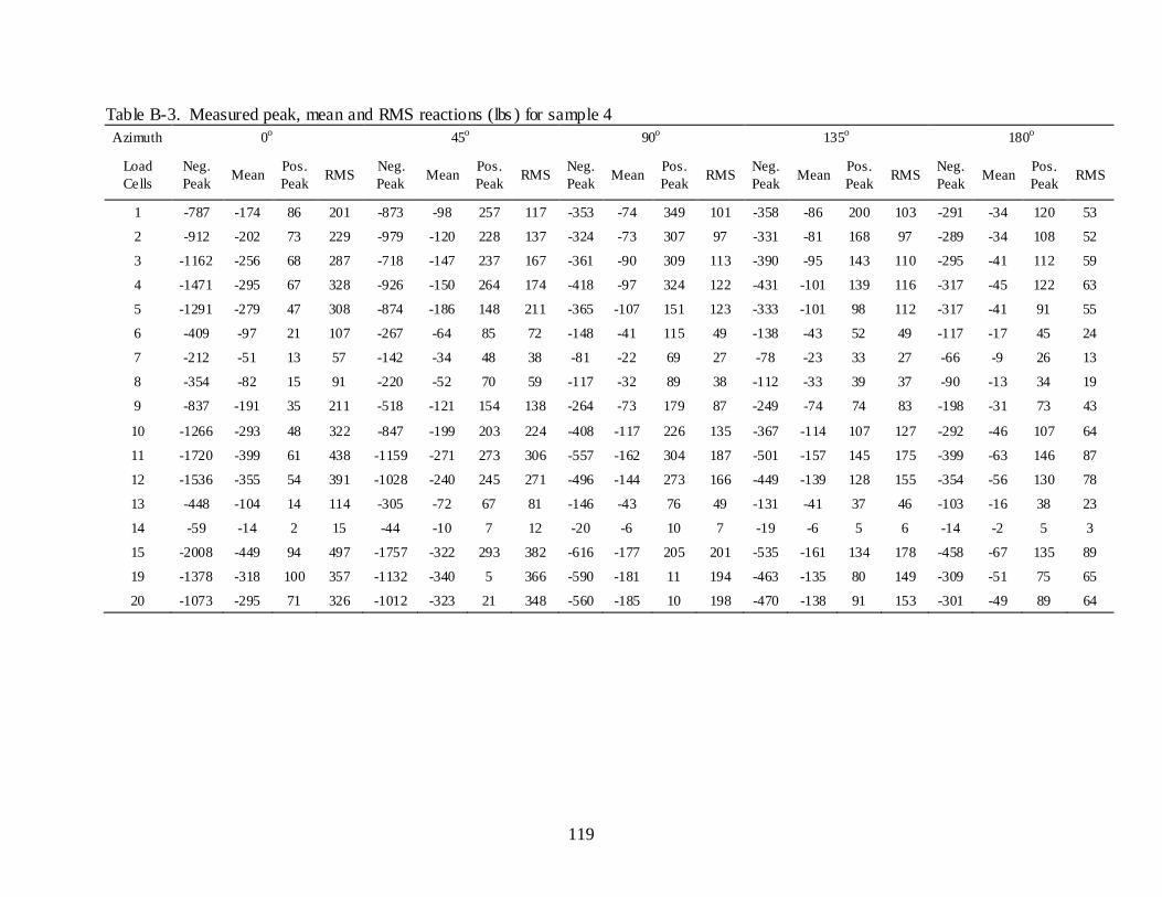
119


Load Cells

Neg. Peak Mean Pos.





Peak RMS

1 -787 -174 86 201 -873 -98 257 117 -353 -74 349 101 -358 -86 200 103 -291 -34 120 53

2 -912 -202 73 229 -979 -120 228 137 -324 -73 307 97 -331 -81 168 97 -289 -34 108 52

3 -1162 -256 68 287 -718 -147 237 167 -361 -90 309 113 -390 -95 143 110 -295 -41 112 59

4 -1471 -295 67 328 -926 -150 264 174 -418 -97 324 122 -431 -101 139 116 -317 -45 122 63

5 -1291 -279 47 308 -874 -186 148 211 -365 -107 151 123 -333 -101 98 112 -317 -41 91 55

6 -409 -97 21 107 -267 -64 85 72 -148 -41 115 49 -138 -43 52 49 -117 -17 45 24

7 -212 -51 13 57 -142 -34 48 38 -81 -22 69 27 -78 -23 33 27 -66 -9 26 13

8 -354 -82 15 91 -220 -52 70 59 -117 -32 89 38 -112 -33 39 37 -90 -13 34 19

9 -837 -191 35 211 -518 -121 154 138 -264 -73 179 87 -249 -74 74 83 -198 -31 73 43

10 -1266 -293 48 322 -847 -199 203 224 -408 -117 226 135 -367 -114 107 127 -292 -46 107 64

11 -1720 -399 61 438 -1159 -271 273 306 -557 -162 304 187 -501 -157 145 175 -399 -63 146 87

12 -1536 -355 54 391 -1028 -240 245 271 -496 -144 273 166 -449 -139 128 155 -354 -56 130 78

13 -448 -104 14 114 -305 -72 67 81 -146 -43 76 49 -131 -41 37 46 -103 -16 38 23

14 -59 -14 2 15 -44 -10 7 12 -20 -6 10 7 -19 -6 5 6 -14 -2 5 3

15 -2008 -449 94 497 -1757 -322 293 382 -616 -177 205 201 -535 -161 134 178 -458 -67 135 89

19 -1378 -318 100 357 -1132 -340 5 366 -590 -181 11 194 -463 -135 80 149 -309 -51 75 65

20 -1073 -295 71 326 -1012 -323 21 348 -560 -185 10 198 -470 -138 91 153 -301 -49 89 64

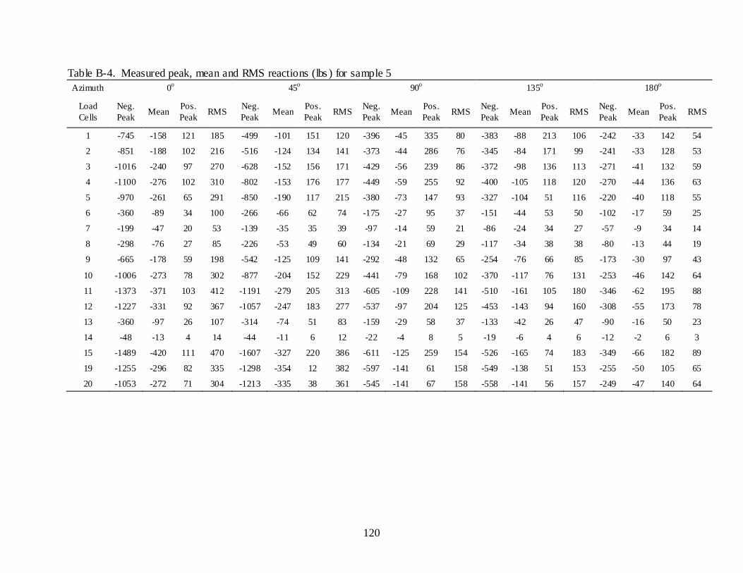
120


Load Cells

Neg. Peak Mean Pos.





Peak RMS

1 -745 -158 121 185 -499 -101 151 120 -396 -45 335 80 -383 -88 213 106 -242 -33 142 54

2 -851 -188 102 216 -516 -124 134 141 -373 -44 286 76 -345 -84 171 99 -241 -33 128 53

3 -1016 -240 97 270 -628 -152 156 171 -429 -56 239 86 -372 -98 136 113 -271 -41 132 59

4 -1100 -276 102 310 -802 -153 176 177 -449 -59 255 92 -400 -105 118 120 -270 -44 136 63

5 -970 -261 65 291 -850 -190 117 215 -380 -73 147 93 -327 -104 51 116 -220 -40 118 55

6 -360 -89 34 100 -266 -66 62 74 -175 -27 95 37 -151 -44 53 50 -102 -17 59 25

7 -199 -47 20 53 -139 -35 35 39 -97 -14 59 21 -86 -24 34 27 -57 -9 34 14

8 -298 -76 27 85 -226 -53 49 60 -134 -21 69 29 -117 -34 38 38 -80 -13 44 19

9 -665 -178 59 198 -542 -125 109 141 -292 -48 132 65 -254 -76 66 85 -173 -30 97 43

10 -1006 -273 78 302 -877 -204 152 229 -441 -79 168 102 -370 -117 76 131 -253 -46 142 64

11 -1373 -371 103 412 -1191 -279 205 313 -605 -109 228 141 -510 -161 105 180 -346 -62 195 88

12 -1227 -331 92 367 -1057 -247 183 277 -537 -97 204 125 -453 -143 94 160 -308 -55 173 78

13 -360 -97 26 107 -314 -74 51 83 -159 -29 58 37 -133 -42 26 47 -90 -16 50 23

14 -48 -13 4 14 -44 -11 6 12 -22 -4 8 5 -19 -6 4 6 -12 -2 6 3

15 -1489 -420 111 470 -1607 -327 220 386 -611 -125 259 154 -526 -165 74 183 -349 -66 182 89

19 -1255 -296 82 335 -1298 -354 12 382 -597 -141 61 158 -549 -138 51 153 -255 -50 105 65

20 -1053 -272 71 304 -1213 -335 38 361 -545 -141 67 158 -558 -141 56 157 -249 -47 140 64

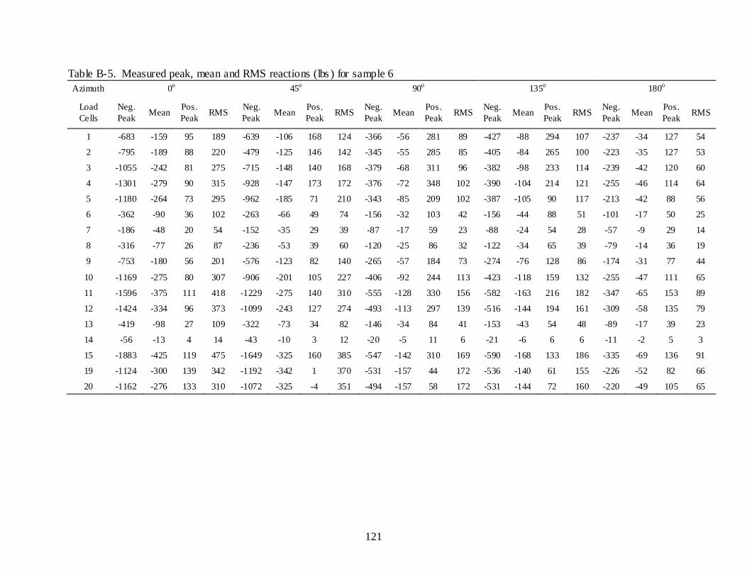
121


Load Cells

Neg. Peak Mean Pos.





Peak RMS

1 -683 -159 95 189 -639 -106 168 124 -366 -56 281 89 -427 -88 294 107 -237 -34 127 54

2 -795 -189 88 220 -479 -125 146 142 -345 -55 285 85 -405 -84 265 100 -223 -35 127 53

3 -1055 -242 81 275 -715 -148 140 168 -379 -68 311 96 -382 -98 233 114 -239 -42 120 60

4 -1301 -279 90 315 -928 -147 173 172 -376 -72 348 102 -390 -104 214 121 -255 -46 114 64

5 -1180 -264 73 295 -962 -185 71 210 -343 -85 209 102 -387 -105 90 117 -213 -42 88 56

6 -362 -90 36 102 -263 -66 49 74 -156 -32 103 42 -156 -44 88 51 -101 -17 50 25

7 -186 -48 20 54 -152 -35 29 39 -87 -17 59 23 -88 -24 54 28 -57 -9 29 14

8 -316 -77 26 87 -236 -53 39 60 -120 -25 86 32 -122 -34 65 39 -79 -14 36 19

9 -753 -180 56 201 -576 -123 82 140 -265 -57 184 73 -274 -76 128 86 -174 -31 77 44

10 -1169 -275 80 307 -906 -201 105 227 -406 -92 244 113 -423 -118 159 132 -255 -47 111 65

11 -1596 -375 111 418 -1229 -275 140 310 -555 -128 330 156 -582 -163 216 182 -347 -65 153 89

12 -1424 -334 96 373 -1099 -243 127 274 -493 -113 297 139 -516 -144 194 161 -309 -58 135 79

13 -419 -98 27 109 -322 -73 34 82 -146 -34 84 41 -153 -43 54 48 -89 -17 39 23

14 -56 -13 4 14 -43 -10 3 12 -20 -5 11 6 -21 -6 6 6 -11 -2 5 3

15 -1883 -425 119 475 -1649 -325 160 385 -547 -142 310 169 -590 -168 133 186 -335 -69 136 91

19 -1124 -300 139 342 -1192 -342 1 370 -531 -157 44 172 -536 -140 61 155 -226 -52 82 66

20 -1162 -276 133 310 -1072 -325 -4 351 -494 -157 58 172 -531 -144 72 160 -220 -49 105 65

122


Load Cells

Neg. Peak Mean Pos.





Peak RMS

1 -826 -159 142 190 -453 -108 176 125 -416 -62 285 92 -416 -91 221 109 -232 -33 136 54

2 -899 -188 147 219 -481 -127 142 144 -395 -61 217 88 -416 -86 164 102 -229 -34 125 52

3 -1003 -240 152 273 -544 -151 122 170 -434 -76 222 102 -373 -100 118 116 -251 -41 132 59

4 -1068 -276 172 312 -729 -150 139 174 -446 -80 266 109 -393 -107 125 122 -251 -44 134 63

5 -1020 -261 95 292 -835 -187 77 212 -409 -93 186 111 -380 -106 57 117 -214 -40 106 55

6 -369 -90 54 102 -219 -67 44 75 -187 -35 79 44 -154 -45 48 51 -108 -17 55 25

7 -205 -47 31 54 -122 -36 27 40 -104 -19 47 24 -86 -25 31 28 -60 -9 31 14

8 -295 -76 42 86 -193 -54 36 60 -144 -27 62 35 -118 -35 32 39 -79 -13 42 19

9 -659 -178 92 200 -484 -125 75 141 -318 -63 142 78 -265 -78 57 87 -171 -30 90 43

10 -998 -273 121 305 -791 -204 99 229 -482 -102 203 122 -410 -120 75 134 -248 -46 130 64

11 -1361 -371 161 416 -1075 -278 135 312 -664 -141 273 169 -564 -165 101 184 -333 -62 177 88

12 -1208 -331 143 370 -958 -246 122 277 -590 -125 246 150 -500 -146 90 163 -294 -56 157 78

13 -351 -97 40 108 -284 -74 34 83 -174 -37 71 44 -148 -43 25 48 -85 -16 46 23

14 -45 -13 5 14 -40 -11 4 12 -24 -5 10 6 -21 -6 3 6 -12 -2 6 3

15 -1549 -420 141 471 -1672 -327 166 387 -650 -157 290 185 -613 -169 64 186 -351 -67 171 89

19 -1259 -293 73 336 -1199 -343 5 371 -576 -166 72 181 -540 -140 39 155 -252 -50 107 64

20 -1118 -272 114 306 -1033 -326 13 353 -570 -168 69 183 -522 -144 49 159 -276 -47 134 64

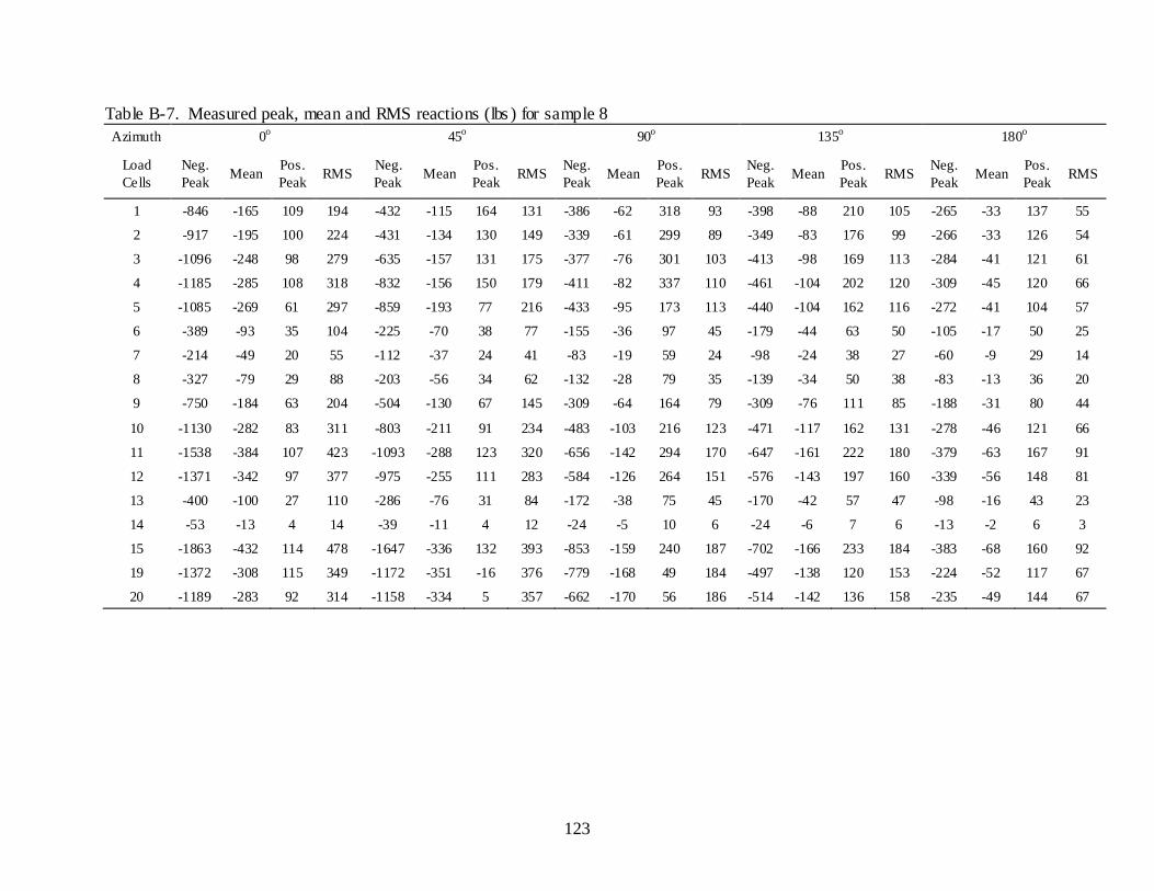
123


Load Cells

Neg. Peak Mean Pos.





Peak RMS

1 -846 -165 109 194 -432 -115 164 131 -386 -62 318 93 -398 -88 210 105 -265 -33 137 55

2 -917 -195 100 224 -431 -134 130 149 -339 -61 299 89 -349 -83 176 99 -266 -33 126 54

3 -1096 -248 98 279 -635 -157 131 175 -377 -76 301 103 -413 -98 169 113 -284 -41 121 61

4 -1185 -285 108 318 -832 -156 150 179 -411 -82 337 110 -461 -104 202 120 -309 -45 120 66

5 -1085 -269 61 297 -859 -193 77 216 -433 -95 173 113 -440 -104 162 116 -272 -41 104 57

6 -389 -93 35 104 -225 -70 38 77 -155 -36 97 45 -179 -44 63 50 -105 -17 50 25

7 -214 -49 20 55 -112 -37 24 41 -83 -19 59 24 -98 -24 38 27 -60 -9 29 14

8 -327 -79 29 88 -203 -56 34 62 -132 -28 79 35 -139 -34 50 38 -83 -13 36 20

9 -750 -184 63 204 -504 -130 67 145 -309 -64 164 79 -309 -76 111 85 -188 -31 80 44

10 -1130 -282 83 311 -803 -211 91 234 -483 -103 216 123 -471 -117 162 131 -278 -46 121 66

11 -1538 -384 107 423 -1093 -288 123 320 -656 -142 294 170 -647 -161 222 180 -379 -63 167 91

12 -1371 -342 97 377 -975 -255 111 283 -584 -126 264 151 -576 -143 197 160 -339 -56 148 81

13 -400 -100 27 110 -286 -76 31 84 -172 -38 75 45 -170 -42 57 47 -98 -16 43 23

14 -53 -13 4 14 -39 -11 4 12 -24 -5 10 6 -24 -6 7 6 -13 -2 6 3

15 -1863 -432 114 478 -1647 -336 132 393 -853 -159 240 187 -702 -166 233 184 -383 -68 160 92

19 -1372 -308 115 349 -1172 -351 -16 376 -779 -168 49 184 -497 -138 120 153 -224 -52 117 67

20 -1189 -283 92 314 -1158 -334 5 357 -662 -170 56 186 -514 -142 136 158 -235 -49 144 67

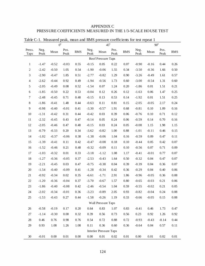
124

APPENDIX C PRESSURE COEFFICIENTS MEASURED IN THE 1/3-SCALE HOUSE TEST

Table C-1. Measured peak, mean and RMS pressure coefficients for test repeat 1 0o 45o 90o

Press. Taps

Neg. Peak Mean Pos.



Peak RMS

Roof Pressure Taps

1 -1.47 -0.52 -0.03 0.55 -0.15 0.05 0.22 0.07 -0.90 -0.16 0.44 0.26

2 -2.42 -0.50 1.05 0.54 -1.90 -0.06 1.55 0.34 -3.50 -0.36 1.66 0.50

3 -2.90 -0.47 1.85 0.51 -2.77 -0.82 1.29 0.90 -3.26 -0.49 1.61 0.57

4 -2.62 -0.44 0.92 0.49 -1.94 -0.56 1.73 0.60 -3.00 -0.54 1.31 0.60

5 -2.05 -0.49 0.08 0.52 -1.54 0.07 1.24 0.20 -1.86 0.01 1.51 0.21

6 -1.85 -0.50 0.22 0.53 -0.04 0.12 0.26 0.12 -1.63 0.06 1.47 0.25

7 -2.48 -0.45 0.71 0.48 -0.15 0.13 0.53 0.14 -1.92 0.01 1.51 0.25

8 -1.86 -0.41 1.48 0.44 -0.63 0.11 0.81 0.15 -2.05 -0.05 2.17 0.24

9 -0.98 -0.40 -0.01 0.41 -3.30 -0.57 1.91 0.68 -0.81 0.10 1.09 0.16

10 -1.31 -0.42 0.31 0.44 -0.42 0.03 0.39 0.06 -0.76 0.10 0.71 0.12

11 -2.32 -0.45 0.43 0.47 -0.14 0.05 0.24 0.06 -0.59 0.14 0.70 0.16

12 -2.05 -0.46 0.47 0.48 -0.15 0.03 0.24 0.05 -0.08 1.15 1.98 1.15

13 -0.79 -0.33 0.20 0.34 -3.62 -0.82 1.00 0.88 -1.01 -0.11 0.46 0.15

14 -1.02 -0.37 -0.06 0.38 -1.38 -0.06 1.04 0.16 -0.59 0.09 0.47 0.11

15 -1.39 -0.41 0.11 0.42 -0.47 -0.08 0.18 0.10 -0.44 0.05 0.42 0.07

16 -1.52 -0.46 0.21 0.48 -0.32 -0.09 0.11 0.10 -0.56 0.07 0.71 0.09

17 -1.03 -0.32 0.01 0.33 -3.18 -1.12 1.08 1.17 -0.41 -0.01 0.77 0.07

18 -1.27 -0.36 -0.05 0.37 -2.53 -0.43 1.64 0.50 -0.32 0.04 0.47 0.07

19 -2.21 -0.45 0.03 0.47 -0.75 -0.38 0.04 0.39 -0.39 0.04 0.36 0.07

20 -1.54 -0.40 -0.09 0.41 -1.28 -0.34 0.42 0.36 -0.29 0.04 0.40 0.06

21 -0.92 -0.34 0.02 0.35 -6.61 -1.71 2.91 1.86 -0.96 -0.05 0.36 0.08

22 -1.20 -0.36 -0.04 0.37 -3.70 -0.67 1.57 0.80 -0.65 -0.03 0.21 0.06

23 -1.86 -0.40 -0.08 0.42 -2.46 -0.54 1.04 0.59 -0.55 -0.02 0.21 0.05

24 -2.02 -0.34 -0.01 0.36 -3.23 -0.89 2.05 0.93 -0.82 -0.04 0.24 0.08

25 -1.53 -0.43 0.27 0.44 -1.58 -0.26 1.19 0.33 -0.66 -0.05 0.15 0.08

Wall Pressure Taps

26 -0.58 -0.19 0.17 0.20 0.64 0.83 1.07 0.83 -0.41 0.46 1.73 0.47

27 -1.14 -0.30 0.00 0.32 0.39 0.56 0.73 0.56 0.23 0.92 1.26 0.92

28 0.46 0.76 0.98 0.76 0.54 0.72 0.88 0.72 -0.93 -0.43 -0.14 0.44

29 0.93 1.08 1.26 1.08 0.11 0.36 0.60 0.36 -0.64 0.04 0.57 0.11

Interior Pressure Taps

30 -0.01 0.00 0.01 0.00 0.00 0.01 0.02 0.01 0.00 0.01 0.02 0.01

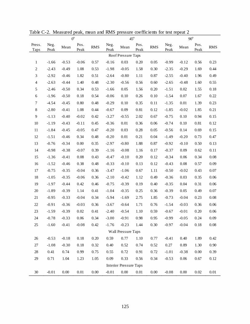
125


Press. Taps

Neg. Peak Mean Pos.



Peak RMS

Roof Pressure Taps

1 -1.66 -0.53 -0.06 0.57 -0.16 0.03 0.20 0.05 -0.99 -0.12 0.56 0.23

2 -2.43 -0.49 1.08 0.53 -1.98 -0.05 1.58 0.30 -2.35 -0.29 1.69 0.44

3 -2.92 -0.46 1.82 0.51 -2.64 -0.80 1.11 0.87 -2.55 -0.40 1.96 0.49

4 -2.63 -0.44 1.40 0.48 -2.30 -0.56 0.56 0.60 -2.65 -0.48 1.60 0.55

5 -2.46 -0.50 0.34 0.53 -1.66 0.05 1.56 0.20 -1.51 0.02 1.55 0.18

6 -1.96 -0.50 0.18 0.54 -0.06 0.10 0.26 0.10 -1.54 0.07 1.67 0.22

7 -4.54 -0.45 0.80 0.48 -0.29 0.10 0.35 0.11 -1.35 0.01 1.39 0.23

8 -2.80 -0.41 1.08 0.44 -0.67 0.09 0.81 0.12 -1.85 -0.02 1.85 0.21

9 -1.13 -0.40 -0.02 0.42 -3.27 -0.55 2.02 0.67 -0.75 0.10 0.94 0.15

10 -1.19 -0.43 -0.11 0.45 -0.36 0.01 0.36 0.06 -0.74 0.10 0.81 0.12

11 -1.84 -0.45 -0.05 0.47 -0.20 0.03 0.28 0.05 -0.56 0.14 0.69 0.15

12 -1.51 -0.46 0.34 0.48 -0.20 0.01 0.21 0.04 -1.49 -0.20 0.73 0.47

13 -0.76 -0.34 0.00 0.35 -2.97 -0.80 1.88 0.87 -0.92 -0.10 0.50 0.13

14 -0.98 -0.38 -0.07 0.39 -1.16 -0.08 1.16 0.17 -0.37 0.09 0.62 0.11

15 -1.36 -0.41 0.08 0.43 -0.47 -0.10 0.20 0.12 -0.34 0.06 0.34 0.08

16 -1.52 -0.46 0.38 0.48 -0.33 -0.10 0.13 0.12 -0.43 0.08 0.57 0.09

17 -0.75 -0.35 -0.04 0.36 -3.47 -1.06 0.67 1.11 -0.50 -0.02 0.43 0.07

18 -1.05 -0.35 -0.06 0.36 -2.10 -0.42 1.12 0.49 -0.36 0.03 0.35 0.06

19 -1.97 -0.44 0.42 0.46 -0.75 -0.39 0.19 0.40 -0.35 0.04 0.31 0.06

20 -1.89 -0.39 1.14 0.41 -1.04 -0.35 0.25 0.36 -0.39 0.05 0.49 0.07

21 -0.95 -0.33 -0.04 0.34 -5.94 -1.69 2.75 1.85 -0.73 -0.04 0.23 0.08

22 -0.91 -0.36 -0.03 0.36 -3.67 -0.64 1.71 0.76 -1.54 -0.03 0.36 0.06

23 -1.59 -0.39 0.02 0.41 -2.40 -0.54 1.10 0.59 -0.67 -0.01 0.20 0.06

24 -0.78 -0.33 0.06 0.34 -3.00 -0.91 0.98 0.95 -0.99 -0.05 0.24 0.09

25 -1.60 -0.41 -0.08 0.42 -1.76 -0.23 1.44 0.30 -0.97 -0.04 0.18 0.08

Wall Pressure Taps

26 -0.53 -0.18 0.18 0.20 0.59 0.77 1.10 0.77 -0.41 0.40 1.89 0.42

27 -1.08 -0.30 0.18 0.32 0.40 0.52 0.74 0.52 0.27 0.89 1.30 0.90

28 0.41 0.74 0.99 0.75 0.55 0.72 0.91 0.72 -1.01 -0.38 0.00 0.39

29 0.71 1.04 1.23 1.05 0.09 0.33 0.56 0.34 -0.53 0.06 0.67 0.12


30 -0.01 0.00 0.01 0.00 -0.01 0.00 0.01 0.00 -0.08 0.00 0.02 0.01

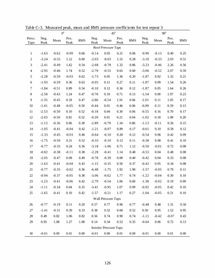
126


Press. Taps

Neg. Peak Mean Pos.



Peak RMS

Roof Pressure Taps

1 -1.63 -0.62 -0.09 0.66 -0.14 0.05 0.21 0.06 -0.90 -0.13 0.40 0.25

2 -3.24 -0.55 1.12 0.60 -2.03 -0.03 1.55 0.28 -3.10 -0.33 2.03 0.51

3 -2.41 -0.49 1.62 0.54 -2.68 -0.78 1.32 0.86 -3.23 -0.46 2.26 0.56

4 -2.95 -0.46 1.74 0.52 -2.70 -0.55 0.65 0.60 -3.06 -0.52 2.07 0.59

5 -2.28 -0.59 -0.03 0.62 -1.73 0.05 1.36 0.20 -1.87 0.02 1.32 0.21

6 -1.93 -0.59 0.36 0.63 -0.05 0.11 0.27 0.11 -1.87 0.09 1.54 0.26

7 -1.84 -0.51 0.89 0.54 -0.10 0.12 0.36 0.12 -1.87 0.05 1.64 0.26

8 -2.58 -0.43 1.24 0.47 -0.78 0.10 0.71 0.13 -1.54 0.00 1.97 0.23

9 -1.35 -0.45 0.18 0.47 -2.86 -0.54 1.91 0.66 -1.01 0.11 1.05 0.17

10 -1.41 -0.48 -0.05 0.50 -0.44 0.01 0.46 0.06 -0.89 0.11 0.59 0.13

11 -2.53 -0.50 0.10 0.52 -0.18 0.04 0.30 0.06 -0.55 0.16 0.70 0.17

12 -2.03 -0.50 0.81 0.52 -0.20 0.01 0.21 0.04 -1.02 0.18 1.08 0.20

13 -1.13 -0.36 0.06 0.38 -2.89 -0.79 1.34 0.86 -1.13 -0.11 0.56 0.15

14 -1.05 -0.41 -0.04 0.42 -1.21 -0.07 0.89 0.17 -0.61 0.10 0.58 0.12

15 -1.33 -0.45 -0.03 0.46 -0.64 -0.10 0.28 0.12 -0.54 0.06 0.42 0.09

16 -1.75 -0.50 0.21 0.52 -0.33 -0.10 0.12 0.11 -0.38 0.08 0.41 0.10

17 -0.77 -0.35 0.24 0.36 -3.18 -1.06 0.71 1.12 -0.50 -0.01 0.72 0.08

18 -0.82 -0.38 -0.11 0.38 -2.28 -0.41 1.14 0.48 -0.53 0.04 0.48 0.08

19 -2.05 -0.47 0.08 0.49 -0.78 -0.39 0.08 0.40 -0.42 0.04 0.33 0.08

20 -1.63 -0.41 -0.04 0.43 -1.15 -0.35 0.50 0.37 -0.42 0.05 0.34 0.08

21 -0.77 -0.35 -0.02 0.36 -6.48 -1.75 1.92 1.90 -1.57 -0.05 0.79 0.11

22 -0.94 -0.37 -0.05 0.38 -3.06 -0.62 1.77 0.74 -1.22 -0.04 0.30 0.10

23 -1.23 -0.41 -0.06 0.42 -2.79 -0.54 1.06 0.60 -1.38 -0.02 0.19 0.09

24 -1.11 -0.34 0.04 0.35 -3.41 -0.95 1.07 0.99 -0.92 -0.05 0.42 0.10

25 -1.65 -0.41 0.10 0.42 -1.57 -0.21 1.17 0.27 -1.04 -0.05 0.21 0.10

Wall Pressure Taps

26 -0.77 -0.19 0.11 0.20 0.57 0.77 0.96 0.77 -0.48 0.48 1.31 0.50

27 -1.41 -0.31 0.39 0.33 0.38 0.52 0.68 0.52 0.50 0.95 1.52 0.95

28 0.49 0.82 1.06 0.82 0.56 0.74 0.90 0.74 -1.11 -0.42 -0.07 0.43

29 0.93 1.08 1.27 1.08 0.14 0.34 0.53 0.35 -0.64 0.06 0.72 0.13


30 -0.01 0.00 0.01 0.00 -0.01 0.00 0.01 0.00 -0.01 0.00 0.01 0.00

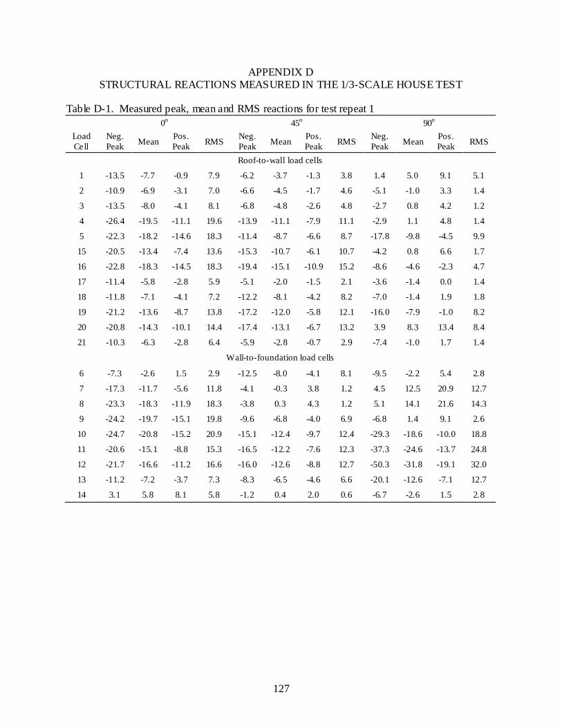
127

APPENDIX D STRUCTURAL REACTIONS MEASURED IN THE 1/3-SCALE HOUSE TEST

Table D-1. Measured peak, mean and RMS reactions for test repeat 1 0o 45o 90o

Load Cell

Neg. Peak Mean Pos.



Peak RMS


1 -13.5 -7.7 -0.9 7.9 -6.2 -3.7 -1.3 3.8 1.4 5.0 9.1 5.1

2 -10.9 -6.9 -3.1 7.0 -6.6 -4.5 -1.7 4.6 -5.1 -1.0 3.3 1.4

3 -13.5 -8.0 -4.1 8.1 -6.8 -4.8 -2.6 4.8 -2.7 0.8 4.2 1.2

4 -26.4 -19.5 -11.1 19.6 -13.9 -11.1 -7.9 11.1 -2.9 1.1 4.8 1.4

5 -22.3 -18.2 -14.6 18.3 -11.4 -8.7 -6.6 8.7 -17.8 -9.8 -4.5 9.9

15 -20.5 -13.4 -7.4 13.6 -15.3 -10.7 -6.1 10.7 -4.2 0.8 6.6 1.7

16 -22.8 -18.3 -14.5 18.3 -19.4 -15.1 -10.9 15.2 -8.6 -4.6 -2.3 4.7

17 -11.4 -5.8 -2.8 5.9 -5.1 -2.0 -1.5 2.1 -3.6 -1.4 0.0 1.4

18 -11.8 -7.1 -4.1 7.2 -12.2 -8.1 -4.2 8.2 -7.0 -1.4 1.9 1.8

19 -21.2 -13.6 -8.7 13.8 -17.2 -12.0 -5.8 12.1 -16.0 -7.9 -1.0 8.2

20 -20.8 -14.3 -10.1 14.4 -17.4 -13.1 -6.7 13.2 3.9 8.3 13.4 8.4

21 -10.3 -6.3 -2.8 6.4 -5.9 -2.8 -0.7 2.9 -7.4 -1.0 1.7 1.4


6 -7.3 -2.6 1.5 2.9 -12.5 -8.0 -4.1 8.1 -9.5 -2.2 5.4 2.8

7 -17.3 -11.7 -5.6 11.8 -4.1 -0.3 3.8 1.2 4.5 12.5 20.9 12.7

8 -23.3 -18.3 -11.9 18.3 -3.8 0.3 4.3 1.2 5.1 14.1 21.6 14.3

9 -24.2 -19.7 -15.1 19.8 -9.6 -6.8 -4.0 6.9 -6.8 1.4 9.1 2.6

10 -24.7 -20.8 -15.2 20.9 -15.1 -12.4 -9.7 12.4 -29.3 -18.6 -10.0 18.8

11 -20.6 -15.1 -8.8 15.3 -16.5 -12.2 -7.6 12.3 -37.3 -24.6 -13.7 24.8

12 -21.7 -16.6 -11.2 16.6 -16.0 -12.6 -8.8 12.7 -50.3 -31.8 -19.1 32.0

13 -11.2 -7.2 -3.7 7.3 -8.3 -6.5 -4.6 6.6 -20.1 -12.6 -7.1 12.7

14 3.1 5.8 8.1 5.8 -1.2 0.4 2.0 0.6 -6.7 -2.6 1.5 2.8

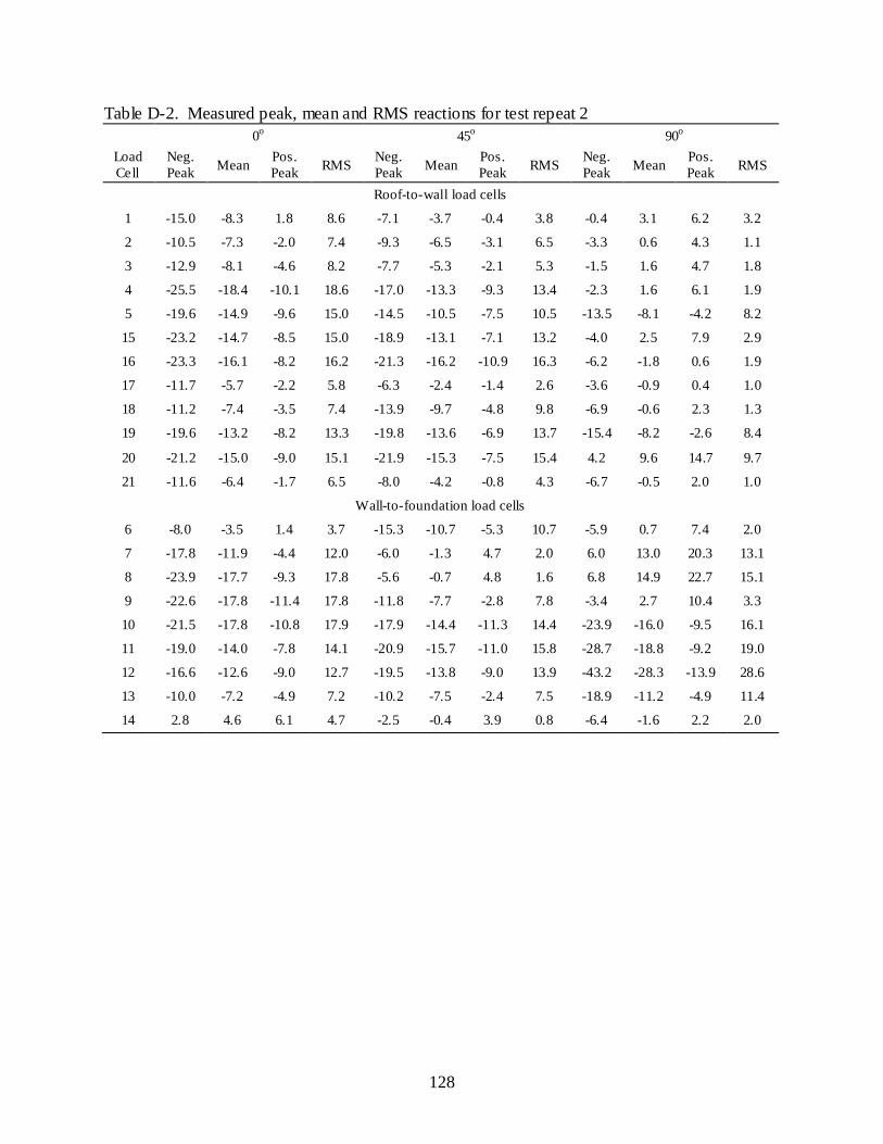
128


Load Cell

Neg. Peak Mean Pos.



Peak RMS


1 -15.0 -8.3 1.8 8.6 -7.1 -3.7 -0.4 3.8 -0.4 3.1 6.2 3.2

2 -10.5 -7.3 -2.0 7.4 -9.3 -6.5 -3.1 6.5 -3.3 0.6 4.3 1.1

3 -12.9 -8.1 -4.6 8.2 -7.7 -5.3 -2.1 5.3 -1.5 1.6 4.7 1.8

4 -25.5 -18.4 -10.1 18.6 -17.0 -13.3 -9.3 13.4 -2.3 1.6 6.1 1.9

5 -19.6 -14.9 -9.6 15.0 -14.5 -10.5 -7.5 10.5 -13.5 -8.1 -4.2 8.2

15 -23.2 -14.7 -8.5 15.0 -18.9 -13.1 -7.1 13.2 -4.0 2.5 7.9 2.9

16 -23.3 -16.1 -8.2 16.2 -21.3 -16.2 -10.9 16.3 -6.2 -1.8 0.6 1.9

17 -11.7 -5.7 -2.2 5.8 -6.3 -2.4 -1.4 2.6 -3.6 -0.9 0.4 1.0

18 -11.2 -7.4 -3.5 7.4 -13.9 -9.7 -4.8 9.8 -6.9 -0.6 2.3 1.3

19 -19.6 -13.2 -8.2 13.3 -19.8 -13.6 -6.9 13.7 -15.4 -8.2 -2.6 8.4

20 -21.2 -15.0 -9.0 15.1 -21.9 -15.3 -7.5 15.4 4.2 9.6 14.7 9.7

21 -11.6 -6.4 -1.7 6.5 -8.0 -4.2 -0.8 4.3 -6.7 -0.5 2.0 1.0


6 -8.0 -3.5 1.4 3.7 -15.3 -10.7 -5.3 10.7 -5.9 0.7 7.4 2.0

7 -17.8 -11.9 -4.4 12.0 -6.0 -1.3 4.7 2.0 6.0 13.0 20.3 13.1

8 -23.9 -17.7 -9.3 17.8 -5.6 -0.7 4.8 1.6 6.8 14.9 22.7 15.1

9 -22.6 -17.8 -11.4 17.8 -11.8 -7.7 -2.8 7.8 -3.4 2.7 10.4 3.3

10 -21.5 -17.8 -10.8 17.9 -17.9 -14.4 -11.3 14.4 -23.9 -16.0 -9.5 16.1

11 -19.0 -14.0 -7.8 14.1 -20.9 -15.7 -11.0 15.8 -28.7 -18.8 -9.2 19.0

12 -16.6 -12.6 -9.0 12.7 -19.5 -13.8 -9.0 13.9 -43.2 -28.3 -13.9 28.6

13 -10.0 -7.2 -4.9 7.2 -10.2 -7.5 -2.4 7.5 -18.9 -11.2 -4.9 11.4

14 2.8 4.6 6.1 4.7 -2.5 -0.4 3.9 0.8 -6.4 -1.6 2.2 2.0

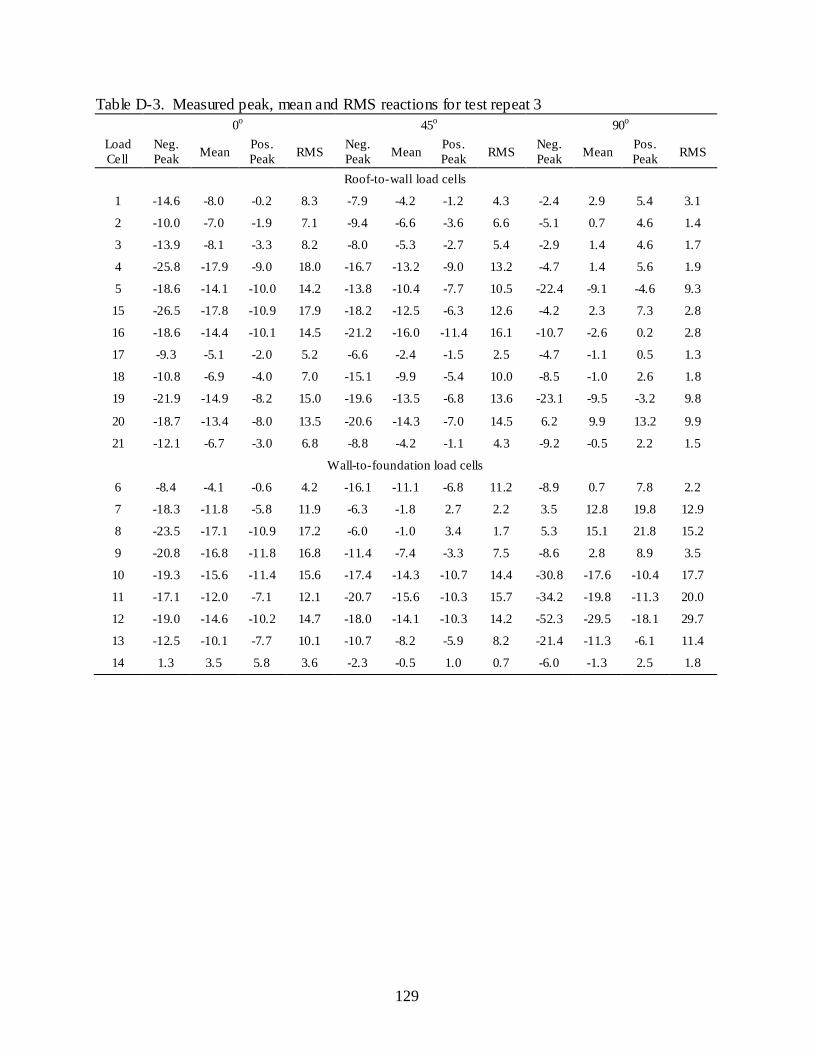
129


Load Cell

Neg. Peak Mean Pos.



Peak RMS


1 -14.6 -8.0 -0.2 8.3 -7.9 -4.2 -1.2 4.3 -2.4 2.9 5.4 3.1

2 -10.0 -7.0 -1.9 7.1 -9.4 -6.6 -3.6 6.6 -5.1 0.7 4.6 1.4

3 -13.9 -8.1 -3.3 8.2 -8.0 -5.3 -2.7 5.4 -2.9 1.4 4.6 1.7

4 -25.8 -17.9 -9.0 18.0 -16.7 -13.2 -9.0 13.2 -4.7 1.4 5.6 1.9

5 -18.6 -14.1 -10.0 14.2 -13.8 -10.4 -7.7 10.5 -22.4 -9.1 -4.6 9.3

15 -26.5 -17.8 -10.9 17.9 -18.2 -12.5 -6.3 12.6 -4.2 2.3 7.3 2.8

16 -18.6 -14.4 -10.1 14.5 -21.2 -16.0 -11.4 16.1 -10.7 -2.6 0.2 2.8

17 -9.3 -5.1 -2.0 5.2 -6.6 -2.4 -1.5 2.5 -4.7 -1.1 0.5 1.3

18 -10.8 -6.9 -4.0 7.0 -15.1 -9.9 -5.4 10.0 -8.5 -1.0 2.6 1.8

19 -21.9 -14.9 -8.2 15.0 -19.6 -13.5 -6.8 13.6 -23.1 -9.5 -3.2 9.8

20 -18.7 -13.4 -8.0 13.5 -20.6 -14.3 -7.0 14.5 6.2 9.9 13.2 9.9

21 -12.1 -6.7 -3.0 6.8 -8.8 -4.2 -1.1 4.3 -9.2 -0.5 2.2 1.5


6 -8.4 -4.1 -0.6 4.2 -16.1 -11.1 -6.8 11.2 -8.9 0.7 7.8 2.2

7 -18.3 -11.8 -5.8 11.9 -6.3 -1.8 2.7 2.2 3.5 12.8 19.8 12.9

8 -23.5 -17.1 -10.9 17.2 -6.0 -1.0 3.4 1.7 5.3 15.1 21.8 15.2

9 -20.8 -16.8 -11.8 16.8 -11.4 -7.4 -3.3 7.5 -8.6 2.8 8.9 3.5

10 -19.3 -15.6 -11.4 15.6 -17.4 -14.3 -10.7 14.4 -30.8 -17.6 -10.4 17.7

11 -17.1 -12.0 -7.1 12.1 -20.7 -15.6 -10.3 15.7 -34.2 -19.8 -11.3 20.0

12 -19.0 -14.6 -10.2 14.7 -18.0 -14.1 -10.3 14.2 -52.3 -29.5 -18.1 29.7

13 -12.5 -10.1 -7.7 10.1 -10.7 -8.2 -5.9 8.2 -21.4 -11.3 -6.1 11.4

14 1.3 3.5 5.8 3.6 -2.3 -0.5 1.0 0.7 -6.0 -1.3 2.5 1.8

130

LIST OF REFERENCES

ASCE/SEI. (2005). "Minimum design loads for buildings and other structures." 7-05, American Society of Civil Engineers, Reston, VA.

Chen, J., Haynes, B. S., and Fletcher, D. F. (2000). "Cobra probe measurements of mean velocities, Reynolds stresses and higher-order velocity correlations in pipe flow." Experimental Thermal and Fluid Science, 21(4), 206-217.

Datin, P. L., and Prevatt, D. O. (2007). "Wind Uplift Reactions at Roof-to-Wall Connections of Wood-Framed Gable Roof Assembly." 12th International Conference on Wind Engineering, Australasian Wind Engineering Society, Cairns, Australia.

Datin, P. L., Prevatt, D. O., and Mensah, A. "Performance Based Wind Engineering: Interaction of Hurricanes with Residential Structures." Engineering Research and Innovation Conference, Honolulu, Hawaii.

Davenport, A. G., Surry, D., and Stathopoulos, T. (1978). "Wind loads on low-rise buildings." Universtiy of Ontario, London, Ontario, Canada.

Doudak, G., McClure, G., Smith, I., Hu, L., and Stathopoulos, T. (2005). "Monitoring Structural Response of a Wooden Light-Frame Industrial Shed Building to Environmental Loads." Journal of Structural Engineering, 131(5), 794-805.

FEMA. (2005). "Mitigation Assessment Team Report: Hurricane Ivan in Alabama and Florida - Observations, Recommendations, and Technical Guidance." FEMA 489, Federal Emergency Management Agency.

Ginger, J. D., and Letchford, C. W. (1993). "Characteristics of large pressures in regions of flow separation." Journal of Wind Engineering and Industrial Aerodynamics, 49, 301-310.

Ginger, J. D., Reardon, G. F., and Whitbread, B. J. (2000). "Wind load effects and equivalent pressures on low-rise house roofs." Engineering Structures, 22(6), 638-646.

Hibbeler, R. C. (2006). Structural Analysis, Pearson Prentice Hall, New Jersey.

Ho, T. C. E., Surry, D., Morrish, D., and Kopp, G. A. (2005a). "The UWO contribution to the NIST aerodynamic database for wind loads on low buildings: Part 1. Archiving format and basic aerodynamic data." Journal of Wind Engineering and Industrial Aerodynamics, 93(1), 1-30.

Ho, T. C. E., Surry, D., Morrish, D., and Kopp, G. A. (2005b). "The UWO contribution to the NIST aerodynamic database for wind loads on low buildings: Part 1. Archiving format and basic aerodynamic data." 93(1), 1-30.

Hooper, J. D., and Musgrove, A. R. (1997). "Reynolds stress, mean velocity, and dynamic static pressure measurement by a four-hole pressure probe." Experimental Thermal and Fluid Science, 15(4), 375-383.

131

Jang, S., Lu, L.-W., Sadek, F., and Simiu, E. (2002). "Database-assisted wind load capacity estimates for low-rise steel frames." Journal of Structural Engineering, 128(12), 1594-1603.

Kopp, G. A., and Chen, Y. (2006). "Database-assisted design of low-rise buildings: Aerodynamic considerations for a practical interpolation scheme." Journal of Structural Engineering, 132(6), 909-917.

Lieblein, J. (1974). "Efficient Methods fo Extreme-Value Methodo logy." National Bureau of Standards, Washington, D.C.

Liu, Z., Prevatt, D. O., Gurley, K. R., Aponte-Bermudez, L., and Reinhold, T. A. (2009). "Field Measurement and Wind Tunnel Simulation of Hurricane Wind Loads on a Single Family Dwelling. " Engineering Structures, (in press).

Main, J. A., and Fritz, W. P. (2006). "Database-Assisted Design for Wind: Concepts, Software, and Examples for Rigid and Flexible Buildings." National Institute of Science and Technology, Gaithersburg, MD.

Martin, K. G., Gupta, R., Prevatt, D. O., Datin, P. L., and van de Lindt, J. W. (2010). "Evaluation of System Effects and Structural Load Paths in a Wood-Framed Structure." Journal of Architectural Engineering, Submitted for review 25 Feb. 2010.

Masters, F., Gurley, K., and Prevatt, D. O. (2008). "Full-Scale Simulation of Turbulent Wind-Driven Rain Effects on Fenestration and Wall Systems." 3rd International Symposium on Wind Effects on Buildings and Urban Environment, Tokyo, Japan.

National Institute of Standards and Technology, N. (2008). "windPressure-DAD software for rigid, gable roof buildings." http://www.itl.nist.gov/div898 /winds/wind_pressure/wind_pressure.htm, Date accessed: 12/20/09.

NIST. (2003). "NIST/SEMATECH e-Handbook of Statistical Methods." National Institute of Standards and Technology. Retrieved March 8, 2007, from http://www.itl.nist.gov/div898/handbook/.

Rigato, A., Chang, P., and Simiu, E. (2001). "Database-assisted design, standardization, and wind direction effects." Journal of Structural Engineering, 127(8), 855-860.

Rosowsky, D., and Schiff, S. (2003). "What are our expectations, objectives, and performance requirements for wood structures in high wind regions?" Natural Hazards Review, 4(3), 144-148.

Rosowsky, D. V., Walsh, T. G., and Crandell, J. H. (2003). "Reliability of residential woodframe construction from 1900 to present." Forest Products Journal, 53(4), 19-28.

http://www.itl.nist.gov/div898/winds/wind_pressure/wind_pressure.htm�

http://www.itl.nist.gov/div898/handbook/�

132

Sadek, F., Diniz, S., Kasperski, M., Gioffre, M., and Simiu, E. (2004). "Sampling Errors in the Estimation of Peak Wind-Induced Interna l Forces in Low-Rise Structures." Journal of Engineering Mechanics, 130(2), 235-239.

Sadek, F., and Simiu, E. (2002). "Peak Non-Gaussian Wind Effects for Database-Assisted Low-Rise Building Design. " Journal of Engineering Mechanics, 128(5), 530-539.

Shepherd, I. C. (1981). "Four-Hole Pressure Probe for Fluid Flow Measurements in Three Dimensions." Journal of Fluids Engineering, Transactions of the ASME, 103(4), 590-594.

Simiu, E., and Miyata, T. (2006). Design of Buildings and Bridges for Wind, A Practical Guide for ASCE-7 Standard Users and Designers of Special Structures, John Wiley & Sons, Inc., New Jersey.

Simiu, E., Sadek, F., Whalen, T. M., Jang, S., Lu, L.-W., Diniz, S. M. C., Grazini, A., and Riley, M. A. (2003). "Achieving safer and more economical buildings through database-assisted, reliability-based design for wind." Journal of Wind Engineering and Industrial Aerodynamics, 91(12-15), 1587-1611.

Simiu, E., and Scanlan, R. H. (1996). Wind Effects on Structures - Fundamentals and Applications to Design, John Wiley & Sons, Inc., New York.

Simiu, E., and Stathopoulos, T. (1997). "Codification of wind loads on buildings using bluff body aerodynamics and climatological data bases." Journal of Wind Engineering and Industrial Aerodynamics, 69-71, 497-506.

St. Pierre, L. M., Kopp, G. A., Surry, D., and Ho, T. C. E. (2005). "The UWO contribution to the NIST aerodynamic database for wind loads on low buildings: Part 2. Comparison of data with wind load provisions." Journal of Wind Engineering and Industrial Aerodynamics, 93(1), 31-59.

Stathopoulos, T. (1979). "Turbulent Wind Action on Low-rise Buildings," Universtiy of Ontario, London, Ontario, London.

Suresh Kumar, K., and Stathopoulos, T. (2000). "Wind loads on low building roofs: a stochastic perspective." Journal of Structural Engineering, 126(8), 944-956.

van de Lindt, J. W., Graettinger, A., Gupta, R., Skaggs, T., Pryor, S., and Fridley, K. J. (2007). "Performance of Wood-Frame Structures during Hurricane Katrina." Journal of Performance of Constructed Facilities, 21(2), 108-116.

Watkins, S., Mousley, P., and Vino, G. "The Development and Use of Dynamic Pressure Probes With Extended Cones of Acceptance (ECA)." 15th Australasian Fluid Mechanics Conference, The University of Sydney, S ydney, Australia.

Whalen, T., Simiu, E., Harris, G., Lin, J., and David, S. (1998). "The use of aerodynamic databases for the effective estimation of wind e ffects in main wind-force resisting

133

systems:: application to low buildings." Journal of Wind Engineering and Industrial Aerodynamics, 77-78, 685-693.

Whalen, T. M., Sadek, F., and Simiu, E. (2002). "Database-assisted design for wind: Basic concepts and software development." Journal of Wind Engineering and Industrial Aerodynamics, 90(11), 1349-1368.

Whalen, T. M., Shah, V., and Yang, J.-S. (2000). "A Pilot Project For Computer-Based Design of Low-Rise Buildings for Wind Loads - The WiLDE-LRS User's Manual." Purdue University, West Lafayette, IN.

Zisis, I., and Stathopoulos, T. (2009). "Wind-Induced C ladd ing and S tructural Loads on Low-Wood Building." Journal of Structural Engineering, 135(4), 437-447.

134

BIOGRAPHICAL SKETCH

Akwasi Frimpong Mensah was born and raised in Takoradi, Ghana. He graduated with a

Bachelor of Science degree in civil engineering from the Kwame Nkrumah University of Science

and Technology in May 2006. He served as a teaching assistant for a year with the same

institution after graduating and later on worked as a Civil/ Structural Engineer with Comptran

Engineering and Planning Associates, Accra for another year. He joined University of Florida in

pursuit of a master degree in August 2008. He anticipates receiving a degree of Master of

Science in Civil Engineering in August 2010. The author hopes to practice as an engineer and

also lecture in the discipline.

Documents

To my parents Mr. & Mrs. P. K. Mensah