To do today: short-run production (only labor variable)

To increase output with a fixed plant, a firm must increase the quantity of labor it uses.

Short-run production: only labor variable

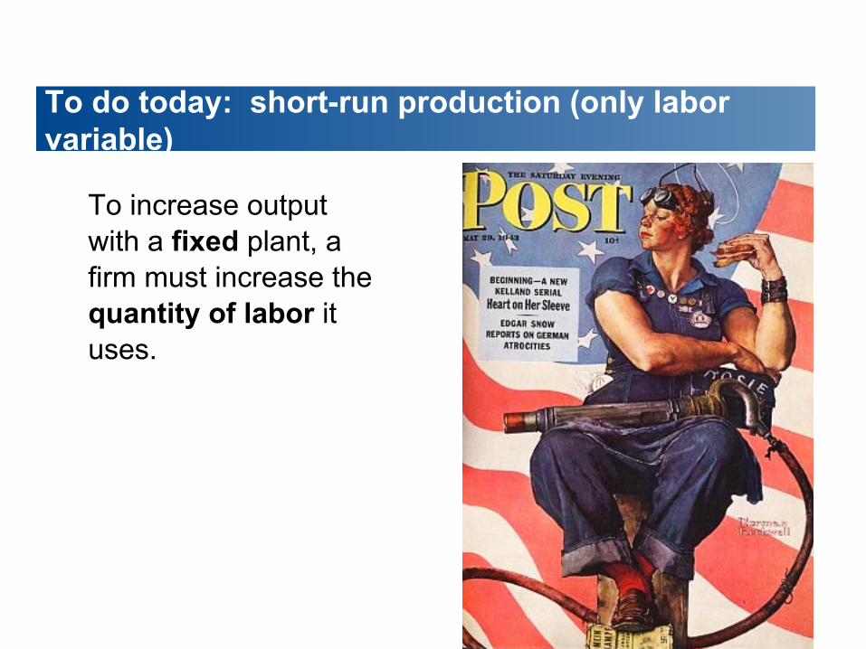
To increase output with a fixed plant, a firm must increase the quantity of labor it uses.

How much will it use?

Requires

•  Total product (TP)

•  Marginal product (MP)

•  Average product (AP)

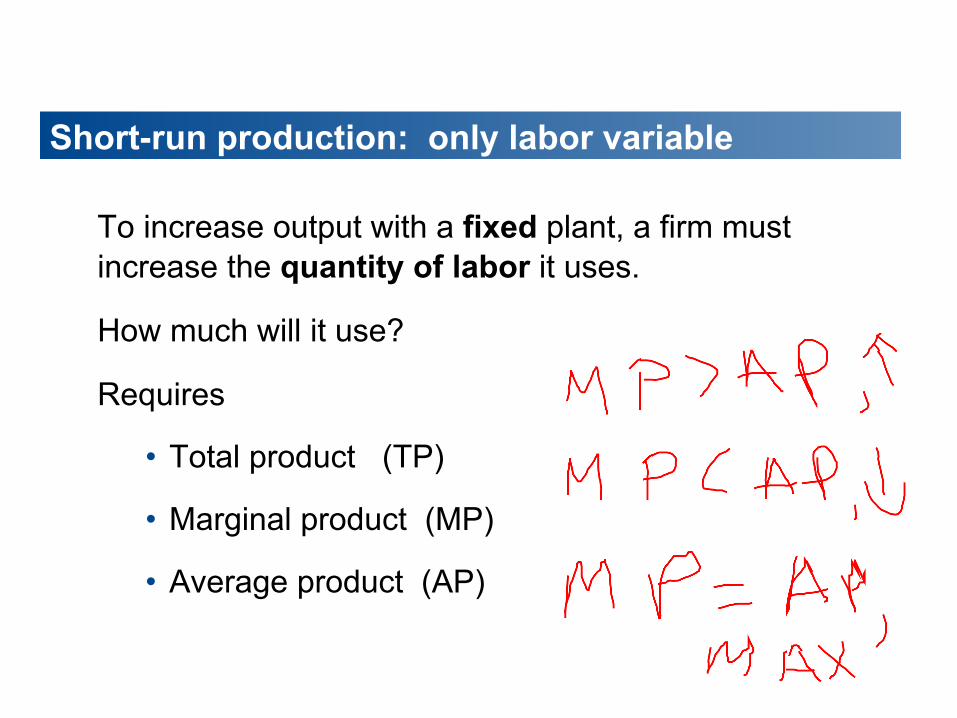
Consequences of the short run

 Add more labor to increase output

 But can’t add more capital goods

Note similarity to total utility!

Points A through H on the curve correspond to the columns of the table.

The TP curve separates attainable points and unattainable points.

Graphing total product

Marginal product: note role of labor!

Marginal product (MP) : change in total product from a one-unit increase in the quantity of labor employed (Ql).

When the quantity of labor increases by more (or less) than one worker, calculate marginal product as

MP Change in TP Change in Ql = ÷

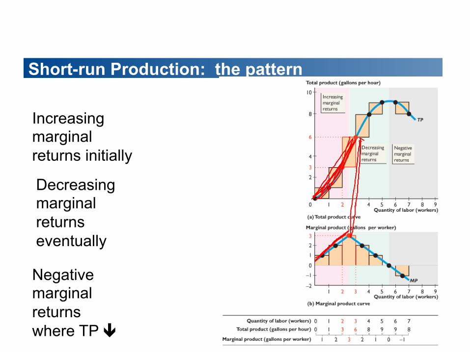
Increasing marginal returns initially

Decreasing marginal returns eventually

Negative marginal returns where TP

Short-run Production: the pattern

ê

Marginal returns: first increasing then decreasing

Increasing marginal returns: from increased specialization and division of labor in the production process.

Decreasing marginal returns: more and more workers use the same equipment and work space.

‘Law” of decreasing marginal returns.

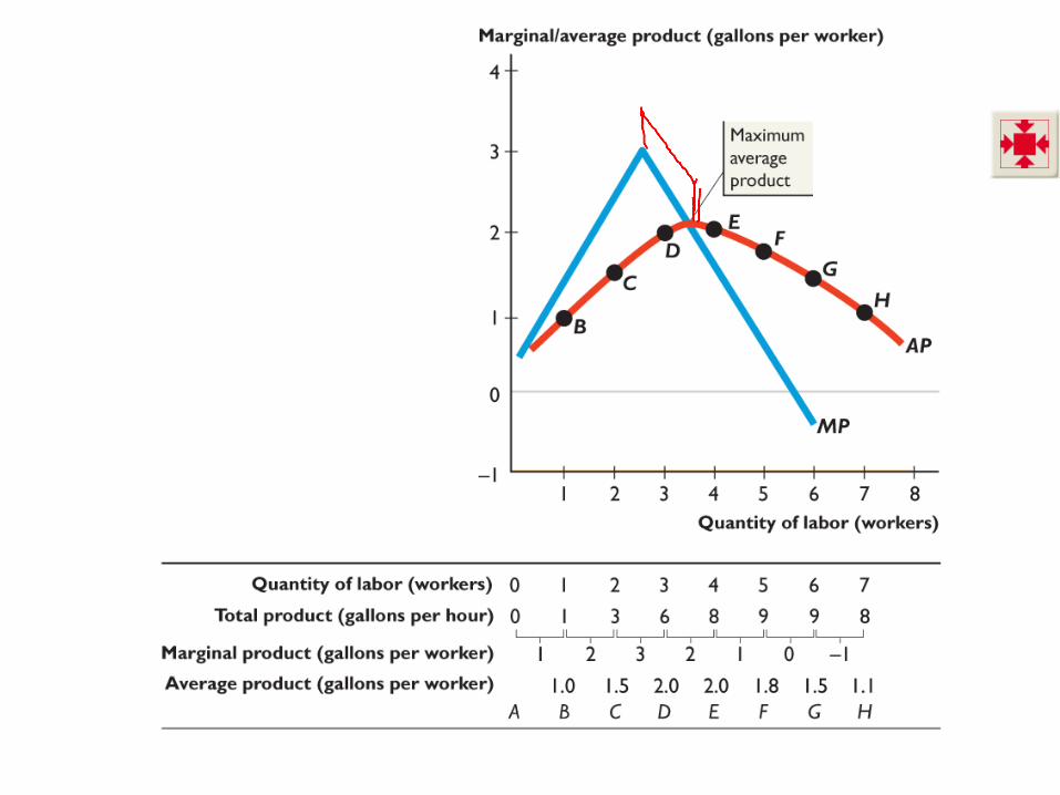
Average product

Like any average – total divided by the number of units

AP = TP ÷ Ql

Another name for average product is productivity.

<iAnnotate iPad User>

Pencil

Short run cost

Costs change with output depending on the shape of three relationships

•  Total cost •  Marginal cost •  Average cost

Fixed and variable costs

Fixed examples: factory building (rent or the mortgage payment), machines (rent or the interest on loan used to buy machines)

Variable examples: workers (wages), electricity to run the machines, office supplies like paper, raw materials like dough and sauce for pizza.

Total cost is the sum of total fixed cost and total variable cost. That is,

TC = TFC + TVC

Remember for what comes next: Fixed does not change with the level of output.

Short run total cost

.

TFC is constant—it graphs as a horizontal line.

TC then also increases as output increases.

TVC increases as output increases.

Graphing short run costs

The vertical distance between the TC curve and the TVC curve is TFC cost

TFC in two places

Marginal cost (MC)

MC: change in total cost that results from a one-unit increase in TP.

She produces one more widget: MC is the cost of this additional unit of output.

.

Average cost: three concepts (from TC)

Average fixed cost (AFC) is total fixed cost per unit of output.

Average variable cost (AVC) is total variable cost per unit of output.

Average total cost (ATC) is total cost per unit of output.

Total and average cost conceps

The average cost concepts are calculated from the total cost concepts as follows:

TC = TFC + TVC

Divide each total cost term by the quantity produced, Q, to give

ATC = AFC + AVC

Q Q Q TC = TFC + TVC

or,

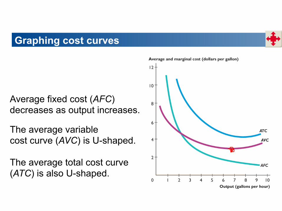
Average fixed cost (AFC) decreases as output increases.

The average variable cost curve (AVC) is U-shaped.

The average total cost curve (ATC) is also U-shaped.

Graphing cost curves

The marginal cost curve (MC) is U-shaped and intersects the average variable cost curve and the average total cost curve at their minimum points.

The vertical distance between ATC and AVC curves is equal to AFC, as illustrated by the two arrows.

Relationships among cost curves

Explaining the shape of the ATC

The shape of the ATC curve combines the shapes of the AFC and AVC curves.

The U shape of the average total cost curve arises from the influence of two opposing forces:

•  Spreading total fixed cost over a larger output •  Decreasing marginal returns

Short run cost and product curves

As productivity decreases, costs rise. This means that cost and product curves are

reverse sides of the coin.

MC curve is linked to its MP curve.

If MP rises, MC falls.

If MP is a maximum, MC is a minimum.

The cost and product curve relationship graphically

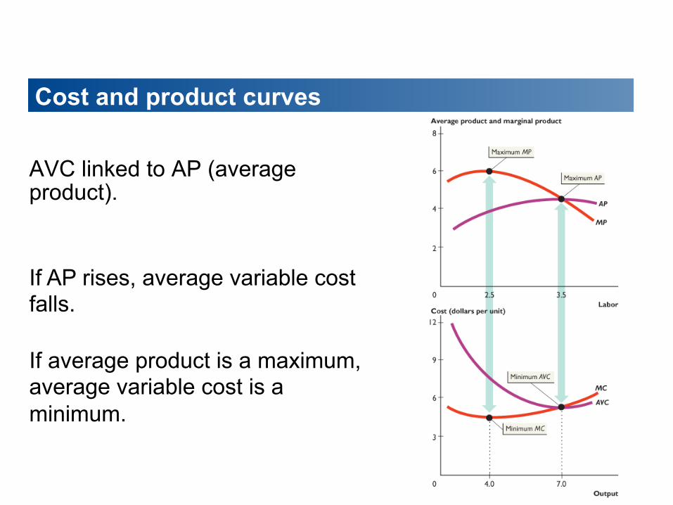
AVC linked to AP (average product).

If AP rises, average variable cost falls.

If average product is a maximum, average variable cost is a minimum.

Cost and product curves

At small outputs, MP and AP é MC and AVC ê At intermediate outputs, MP ê MC é APé AVC ê

At large outputs, MP and AP ê MC and AVC é

Cost and product curves

Shifts in cost curves: what technology does

A technological change that increases productivity shifts the TP curve upward.

It also shifts the MP curve and the AP curve upward.

Why? An advance in technology lowers the AC and MC and so shifts the short-run cost curves downward.

Shifts: prices of factors of production

How the curves shift depends on which resource price changes.

An increase in rent or another component of FC •  Shifts the fixed cost curves (TFC and AFC) upward. •  Shifts the total cost curve (TC) upward. •  Leaves the variable cost curves (AVC and TVC) and

the marginal cost curve (MC) unchanged.

Shifts: variable costs

An increase in the wage rate or another component of variable cost

•  Shifts the variable curves (TVC and AVC) upward. •  Shifts the marginal cost curve (MC) upward. •  Leaves the fixed cost curves (AFC and TFC)

unchanged.