TO APPEAR IN SPECIAL ISSUE: ADVANCES IN …becs.aalto.fi/~ssarkka/pub/inf-bayes-draft.pdfTO APPEAR IN SPECIAL ISSUE: ADVANCES IN KERNEL-BASED LEARNING FOR SIGNAL PROCESSING IN THE

TO APPEAR IN SPECIAL ISSUE: ADVANCES IN KERNEL-BASED LEARNING FOR SIGNAL PROCESSING IN THE IEEE SIGNAL PROCESSING MAGAZINE 1

Spatio-Temporal Learning via Infinite-DimensionalBayesian Filtering and SmoothingSimo Sarkka, Senior Member, IEEE, Arno Solin, and Jouni Hartikainen

Abstract—Gaussian process based machine learning is a pow-erful Bayesian paradigm for non-parametric non-linear regres-sion and classification. In this paper, we discuss connections ofGaussian process regression with Kalman filtering, and presentmethods for converting spatio-temporal Gaussian process regres-sion problems into infinite-dimensional state space models. Thisformulation allows for use of computationally efficient infinite-dimensional Kalman filtering and smoothing methods, or moregeneral Bayesian filtering and smoothing methods, which reducesthe problematic cubic complexity of Gaussian process regressionin the number of time steps into linear time complexity. Theimplication of this is that the use of machine learning models insignal processing becomes computationally feasible, and it opensthe possibility to combine machine learning techniques with sig-nal processing methods.

Index Terms—Gaussian process, machine learning, infinite-dimensional Bayesian filtering and smoothing, spatio-temporalprocess, state space model

I. INTRODUCTION

SPATIO-temporal Gaussian processes, or Gaussian fields,arise in many disciplines such as spatial statistics and krig-

ing, machine learning, physical inverse problems, and signalprocessing [1], [2], [3], [4], [5]. In these applications, we areinterested in doing statistical inference on the dynamic state ofthe whole field based on a finite set of indirect measurementsas well as estimating the properties (i.e., the parameters) ofthe underlying process (or field). For example, in electricalimpedance tomography (EIT) problems [4] we try to recon-struct the resistance field of a body based on voltages inducedby injected currents. In spatial statistics typical problems areprediction of wind, precipitation or ocean currents based onfinite sets of measurements [1].

In Gaussian process based Bayesian machine learning [2]Gaussian processes are used as non-parametric priors for re-gressor functions, and the space and time variables take theroles of input variables of the regressor function. Learning inthese non-parametric models amounts to computation of theposterior distribution of the Gaussian process conditioned ona set of measurements and estimation of the parameters of thecovariance function of the process.

Gaussian process regression can also be seen as a kernelmethod, where the covariance function of the Gaussian processserves as the kernel of the corresponding reproducing kernelHilbert space (RKHS) [2]. In this paper we do not directly

S. Sarkka and A. Solin are with the Department of Biomedical Engineeringand Computational Science (BECS), Aalto University, 02150 Espoo, Finlande-mail: { simo.sarkka, arno.solin }@aalto.fi.

J. Hartikainen is with Rocsole Ltd, 70211 Kuopio, FinlandManuscript received February 6, 2013; revised February 6, 2013.

utilize the RKHS formalism, but instead, work in its mathe-matical dual [6], in the stochastic process formalism. The ad-vantage of this is that it enables us to utilize the vast numberof methods developed for inference on stochastic processes.

In classical signal processing and stochastic control, Gaus-sian processes are commonly used for modeling temporal phe-nomena in form of stochastic differential equations (SDE) [7]and the inference procedure is usually solved using Kalmanfilter type of methods [5]. These models are typically basedon physical, electrical or mechanical principles, which can berepresented in form of differential equations. Stochasticity inthese systems is in form of a white noise process acting as anunknown forcing term. It is also possible to use more generalGaussian process models to better model the forcing termsin such systems. This is the underlying idea in latent forcemodels (LFM), which have many applications, for example,in biology, human tracking and satellite navigation [8], [9].

A central practical problem in the Gaussian process regres-sion context as well as in more general statistical inverse prob-lems is the cubic O(N3) computational complexity in thenumber of measurements N . In the spatio-temporal setting,when we obtain, say, M measurements per time step and thetotal number of time steps is T , this translates into a cubiccomplexity in space and time O(M3 T 3). This is problematicin signal processing, because there we usually are interestedin processing long (unbounded) time series and thus it is nec-essary to have linear complexity in time. This is also the rea-son for the popularity of SDE models and state space modelsin signal processing—their inference problem can be solvedwith Kalman (or Bayesian) filters and smoothers which havea linear O(T ) time complexity.

Due to the computational efficiency of Kalman filtersand smoothers, it is beneficial to reformulate certain spatio-temporal Gaussian process regression problems as Kalman fil-tering and smoothing problems. The aim of this paper is toshow when and how this is possible. We also present a numberof analytical examples, and apply the methodology to predic-tion of precipitation and to processing of fMRI brain imagingdata.

The described methods will be mainly based on the articlesHartikainen & Sarkka [10] and Sarkka & Hartikainen [11].However, the idea of reducing the computational complexityof Gaussian process regression (or equivalent kriging) via re-duction into SDE form has also been suggested by Lindgrenet al. [12], and filtering and smoothing type of methods havebeen applied to spatio-temporal context before [13], [4], [14].Applying recursive Bayesian methods to on-line learning inGaussian process regression has also been proposed, for ex-ample, in [15] and they are also closely related to kernel re-


cursive least squares (KRLS) algorithms [16], [17]. Infinite-dimensional filtering and smoothing methods as such date backto the 60’s–70’s [18]. An alternative general way of copingwith the computational complexity problem is by using sparseapproximations [19], [2], but here we will concentrate on thestate space approach.

The structure of this paper is as follows. In Section II wedescribe how Gaussian processes are used in regression andKalman filtering, and what the idea behind combining the ap-proaches is. In Section III we present methods for convertingGaussian process regression models into state space modelswhich are suitable for Kalman filtering and smoothing meth-ods. In Section IV we discuss how the inference procedure canbe done in practice, how it can be extended to non-linear andnon-Gaussian models and parameter estimation, and finally inSection V, we present two example applications.

II. GAUSSIAN PROCESSES IN REGRESSION AND KALMANFILTERING

A. Definition of a Gaussian Process

A Gaussian process is a random function f(ξ) with d-dimensional input ξ such that any finite collection of randomvariables f(ξ1), . . . , f(ξn) has a multidimensional Gaussiandistribution. Note that when d > 1, what we here call Gaus-sian processes are often called Gaussian fields, but here wewill always use the term process, regardless of the dimension-ality d.

A Gaussian process can be defined in terms of a mean m(ξ)and covariance function k(ξ, ξ′):

m(ξ) = E[f(ξ)]

k(ξ, ξ′) = E[(f(ξ)−m(ξ)) (f(ξ′)−m(ξ′))].(1)

The joint distribution of an arbitrary finite collection of randomvariables f(ξ1), . . . , f(ξn) is then multidimensional Gaussian:f(ξ1)

...f(ξn)

∼ N

m(ξ1)

...m(ξn)

,

k(ξ1, ξ1) . . . k(ξ1, ξn)...

. . .k(ξn, ξ1) k(ξn, ξn)

.

(2)In the same way as a function can be considered as an infinite-long vector consisting of all its values at each input, one way tothink about a Gaussian process is to consider it as an infinite-dimensional limit of a Gaussian random vector. The input vari-able then serves as the element index in this infinite-long ran-dom vector.

A Gaussian process is stationary if its mean is constant andthe two-argument covariance function is of the form

k(ξ, ξ′) = C(ξ′ − ξ), (3)

where C(ξ) is another function, the stationary covariancefunction of the process.

In spatial Gaussian processes, we have ξ = x, where xcorresponds to the input of the random function in Gaussianprocess regression or, for example, a spatial location in geo-statistics or physical inverse problems. In temporal Gaussianprocesses typically arising in signal processing, ξ = t, wheret is the time variable. In spatio-temporal problems ξ = (x, t),

where x and t are the space (or input) and time variables,respectively.

B. Gaussian Process Regression

Gaussian process regression is a way to do non-parametricregression with Gaussian processes. Assume that we want topredict (interpolate) the values of an unknown scalar valuedfunction with d-dimensional input:

y = f(x) (4)

at a certain test point x∗, based on a training set consisting ofa finite number of observed input-output pairs {(xi, yi) : i =1, . . . , N}. Instead of postulating a parametric form of thefunction f(x,θ) as in parametric regression and estimatingthe parameters θ, in Gaussian process regression, we assumethat the function f(x) is a sample from Gaussian process witha given mean m(x) and covariance function k(x,x′). This isdenoted as follows:

f(x) ∼ GP(m(x), k(x,x′)). (5)

In Gaussian process regression, we typically use stationarycovariance functions and assume that the mean is identicallyzero m(x) = 0. A very common choice of covariance functionis the squared exponential covariance function

k(x,x′) = s2 exp

(− 1

2l2||x− x′||2

), (6)

which has the property that the resulting sample functions arevery smooth (infinitely differentiable). The parameters l and sthen define how smooth the function actually is and what isthe magnitude of values that we should expect.

The underlying idea in Gaussian process regression isthat the correlation structure introduces dependencies betweenfunction values at different inputs. Thus the function values atthe observed points give information also of the unobservedpoints. For example, the squared exponential covariance func-tion above says that when the inputs are close to each other,also the function values should be close to each other. Thisis equivalent to saying that the function values with similarinputs should have a stronger correlation than function valueswith dissimilar inputs, which is exactly what the above covari-ance function states.

In statistical estimation problems it is often assumed that themeasurements are not perfect, but instead, they are corruptedby certain additive Gaussian noise. That is, the measurementsare modeled as

yi = f(xi) + εi, εi ∼ N(0, σ2), (7)

where εi are IID random variables, a priori independent of theGaussian process f(x). Now, we are interested in computingan estimate of the value of the “clean” function f(x∗) at testpoint x∗.

The key thing is now to observe that the jointdistribution of the test point and the training points(f(x∗), f(x1), . . . , f(xN )) is Gaussian with known statis-tics (this follows from the definition of a Gaussian pro-cess). Because the measurement model (7) is linear-Gaussian,


the joint distribution of the test point and the measurements(f(x∗), y1, . . . , yN ) is Gaussian with known statistics as well.As everything is Gaussian, we can compute the conditionaldistribution of f(x∗) given the observations y1, . . . , yN byusing the well-known computational rules for Gaussian distri-butions. The result can be expressed as

p(f(x∗) | y1, . . . , yN ) = N(f(x∗) |µ(x∗), V (x∗)), (8)

where the posterior mean µ(x∗) is a function of the train-ing inputs and the measurements, and the posterior varianceV (x∗) is a function of the training inputs (see, [2] for details).However, it turns out that the computational complexity of theequations is O(N3), because of an N × N -matrix inversionappearing in both the mean and covariance equations.

A useful way to rewrite the Gaussian process regressionproblem is in the form

f(x) ∼ GP(m(x), k(x,x′))

y = Hf(x) + ε, ε ∼ N(0,Σ),(9)

where Σ = σ2 I, and the linear operator H picks the trainingset inputs among the function values:

Hf(x) = (f(x1), . . . , f(xN )). (10)

This problem can be seen as a infinite-dimensional version ofthe following Bayesian linear regression problem:

f ∼ N(m,K)

y = Hf + ε,(11)

where f is a vector with Gaussian prior N(m,K), and matrixH is constructed to pick those elements of the vector f thatwe actually observe. Solving the infinite-dimensional linearregression problem in Equation (9) analogously to the finite-dimensional problem in Equation (11), leads to the Gaussianprocess regression solution (cf. [11]). We could also replacethe operator H with a more general linear operator whichwould allow us to solve statistical inverse problems under theGaussian process regression formalism [20].

C. Kalman Filtering and SmoothingKalman filtering is considered with statistical inference on

state space models of the form

df(t)

dt= Af(t) + Lw(t)

yk = Hf(tk) + εk,(12)

where k = 1, . . . , T , and A, L, and H are given matrices,εk is a vector of Gaussian measurement noises, and w(t) is avector of white noise processes. A white noise process refersto a zero mean Gaussian random process, where each pair ofvalues w(t) and w(t′) are uncorrelated whenever t 6= t′.

Because f(t) is a solution to a linear differential equationdriven by Gaussian noise, it is a Gaussian process. It is alsopossible to compute the corresponding covariance function off(t) (see, e.g., [10]), which gives the equivalent covariancefunction based formulation. We can also construct almost anycovariance function for a single selected component of thestate provided that we augment the state to contain a numberof derivatives of the selected state component as well [10].

Location(x) Ti

me(t)

f(x

,t)

Covariancek(x, t; x′, t′)

(a) Covariance function view

Location(x) Ti

me(t)

f(x

,t)

The state at time t

(b) State space model view

Fig. 1. (a) In the covariance function based representation the spatio-temporalfield is considered “frozen” and we postulate the covariance between twospace–time points. (b) In the state space model based description we constructa differential equation for the temporal behavior of a sequence of “snapshots”of the spatial field.

Because the solution of a stochastic differential equation isa Markovian process, it allows for linear time computation ofthe posterior distribution of any unobserved test point f(t∗).The computational algorithms for this are the Kalman filter andRauch–Tung–Striebel (RTS) smoother algorithm. The Kalmanfilter and RTS smoother can be used for computing the meanand covariance of the following distribution for arbitrary t inlinear time complexity:

p(f(t) |y1, . . . ,yT ) = N(f(t) |ms(t),Ps(t)). (13)

Thus we can now pick the time point t = t∗ to obtain theposterior distribution of f(t∗).

D. Combining the ApproachesSpatio-temporal Gaussian process regression is considered

with models of the formf(x, t) ∼ GP(0, k(x, t;x′, t′))

yk = Hkf(x, tk) + εk,(14)

which we have already written in form similar to Equation (9).As mentioned in the previous section, it is possible to force

almost any covariance function of a given state component ofa state space model provided that we augment the state witha sufficient number of time derivatives as well. We can nowuse this idea to formulate a hybrid model, where the temporalcorrelation in the above model is represented as a stochasticdifferential equation kind of model and the spatial correlationis injected into the model by selecting the matrices in themodel properly. In fact, we need to let the spatial dimensionto take the role of an additional vector element index, whichleads to the infinite-dimensional state space model

∂f(x, t)

∂t= A f(x, t) + Lw(x, t)

yk = Hk f(x, tk) + εk,(15)

where the state f(x, t) at time t consists of the whole func-tion x 7→ f(x, t) and a suitable number its time derivatives.This model is now an infinite-dimensional Markovian type ofmodel which allows for linear-time inference with the infinite-dimensional Kalman filter and RTS smoother.


The philosophical difference between the covariance func-tion based model in Equation (14) and the state space modelin Equation (15) is illustrated in Figure 1. In the state spacemodel formulation we think that we have a field that propa-gates forward in time whereas in the covariance based formu-lation we just compute covariances between space–time pointsof a “frozen” field.

III. CONVERTING COVARIANCE FUNCTIONS TO STATESPACE MODELS

A. Covariance Functions of Stochastic Differential Equations

One useful way to construct Gaussian processes is as so-lutions to nth order stochastic linear differential equations ofthe form

andnf(t)

dtn+ · · ·+ a1

df(t)

dt+ a0 f(t) = w(t), (16)

where the driving function w(t) is a zero-mean continuous-time Gaussian white noise process. The solution process f(t),a random function, is a Gaussian process, because w(t) isGaussian and the solution of a linear differential equation is alinear operation on the input.

If we take the formal Fourier transform of Equation (16)and solve for the Fourier transform of the process F (i ω), weget

F (iω) =

(1

an (i ω)n + · · ·+ a1 (i ω) + a0

)︸︷︷︸

G(i ω)

W (i ω), (17)

where W (i ω) is the (formal) Fourier transform of the whitenoise. The above equation can be interpreted such that theprocess F (i ω) is obtained by feeding white noise through asystem with the transfer function G(i ω).

From the above description it is now easy to calculate thecorresponding (power) spectral density of the process, whichis just the square of the absolute value of the Fourier trans-form of the process. If we denote the spectral density of whitenoise |W (i ω)|2 = qc, the spectral density of the process is

S(ω) = qc |G(i ω)|2, (18)

where the key factor is to observe that it has the form

S(ω) =constant

polynomial in ω2. (19)

Thus we can conclude that for an nth order random differ-ential equation of the form (16) the spectral density has therational function form.

The classical Wiener–Khinchin theorem states that the sta-tionary covariance function of the process is given by the in-verse Fourier transform of the spectral density:

C(t) = F−1[S(ω)] =1

2π

∫S(ω) exp(i ω t) dω, (20)

and thus the corresponding covariance function is

k(t, t′) = C(t− t′). (21)

Note that the stochastic differential equation (16) can also beequivalently represented in the following state space form. Ifwe define f = (f, df/dt, . . . ,dn−1f/dtn−1), then we have

df(t)

dt=

0 1

. . . . . .0 1

−a0 −a1 . . . −an−1

︸︷︷︸

A

f(t) +

0...01

︸︷︷︸

L

w(t).

(22)Recall that the scalar function f(t) is just the first compo-

nent of the vector f(t). Thus if we assume that we measurenoise corrupted values yk of f(tk) at points t1, . . . , tN , wecan write this as

yk =(1 0 · · · 0

)︸︷︷︸H

f(t) + εk, (23)

which indeed is a model of the form (12).Thus if we apply the Kalman filter and smoother to the

state space model described by the Equations (22) and (23)we will get the same result as if we applied Gaussian processregression equations to the covariance function defined by theEquation (20). In that sense the representations are equivalent.However, if the number of time steps is T , then the computa-tional complexity of the Kalman filter and smoother is O(T ),whereas the complexity of Gaussian process regression solu-tion is O(T 3). Thus the state space formulation has a hugecomputational advantage, at least when the number of timesteps is large.

In fact, we do not need to restrict ourselves to spectral den-sities of the all-pole form (19), but the transfer function inEquation (17) can be allowed to have the more general form

G(i ω) =bm (i ω)m + · · ·+ b1 (i ω) + b0an (i ω)n + · · ·+ a1 (i ω) + a0

, (24)

where the numerator order is strictly lower than the denomi-nator order m < n with an 6= 0 (i.e., the transfer function isproper). The spectral density then has the more general form

S(ω) =mth order polynomial in ω2

nth order polynomial in ω2, (25)

where the order of the numerator is again lower than the de-nominator’s.

In control theory [21], there exists a number of methods toconvert a transfer function of form (24) into an equivalent statespace model. The procedure which we used above roughlycorresponds to the so called controller canonical form of thestate space model. Another option is, for example, the observercanonical form. In these representations the state variables arenot necessarily pure time derivatives anymore. Anyway, oncewe have the transfer function, we can always convert it into astate space model.

B. From Temporal Covariance Functions to State Space Mod-els

An interesting question is now that if we are given a covari-ance function k(t, t′), how can we find a state space modelwhere one of the state components has this covariance func-tion? We will assume that the process is stationary and thuswe can equivalently say that we want to find a state spacemodel with a component having a stationary covariance func-tion C(t) such that k(t, t′) = C(t− t′).


The procedure to convert a covariance function into statespace model is the following [10]:

1) Compute the corresponding spectral density S(ω) bycomputing the Fourier transform of C(t).

2) If S(ω) is not a rational function of the form (25), thenapproximate it with such a function. This approximationcan be formed using, for example, Taylor series expan-sions or Pade approximants.

3) Find a stable rational transfer function G(i ω) of theform (24) and constant qc such that

S(ω) = G(i ω) qcG(−i ω). (26)

The procedure for finding a stable transfer function iscalled spectral factorization. One method to do that isoutlined later in this section.

4) Use the methods from control theory [21] to convert thetransfer function model into an equivalent state spacemodel. The constant qc will then be the spectral densityof the driving white noise process.

An example of the above procedure is presented in Exam-ple 1 for the Matern covariance function. However, above werequired the transfer function G(i ω) to be stable. A transferfunction corresponds to a stable system if and only if all of itspoles (zeros of the denominator) are in the upper half of thecomplex plane. We also want the transfer function to be min-imum phase, which happens when the zeros of the numeratorare also in the upper half plane.

The procedure to find such a transfer function is called spec-tral factorization. One simple way to do that is the following:• Compute the roots of the numerator and denominator

polynomials of S(ω). The roots will appear in pairs,where one member of the pair is always the complexconjugate of the other.

• Construct the numerator and denominator polynomials ofthe transfer function G(i ω) from the positive-imaginary-part roots only.

If the spectral density does not already have a rational func-tion form, the above procedures only lead to approximations.One example of a covariance function which does not have arational spectral density is the squared exponential covariancefunction in Equation (6). However, its spectral density can bewell approximated with low order rational functions. This isdemonstrated in Example 2.

C. State Space Representation of Spatio-Temporal GaussianProcesses

Let’s now consider the question of representing a spatio-temporal covariance function k(x, t;x′, t′) in state space form.Assuming that the covariance function is stationary we canconcentrate on the corresponding stationary covariance func-tion C(x, t). The space–time Fourier transform then gives thecorresponding spectral density S(ωx, ωt).

If we consider ωx fixed, then ωt 7→ S(ωx, ωt) can be con-sidered as a spectral density of a temporal process which isparametrized with ωx. Assume for simplicity that the func-tion ωt 7→ S(ωx, ωt) has the form of a constant divided bypolynomials (19). This implies that there exists an nth order

Example 1 (1D Matern covariance function). The isotropicand stationary (τ = |t−t′|) covariance function of the Maternfamily can be given as

C(τ) = σ2 21−ν

Γ(ν)

(√2ν

τ

l

)νKν

(√2ν

τ

l

),

where ν, σ, l > 0 are the smoothness, magnitude and lengthscale parameters, and Kν(·) the modified Bessel function (see,e.g., [2]). The spectral density is of the form

S(ω) ∝(λ2 + ω2

)−(ν+1/2),

where λ =√

2ν/l. Thus the spectral density can be factoredas S(ω) ∝ (λ+ i ω)

−(p+1)(λ− i ω)

−(p+1), where ν = p +1/2. The transfer function of the corresponding stable part is

G(i ω) = (λ+ i ω)−(p+1)

.

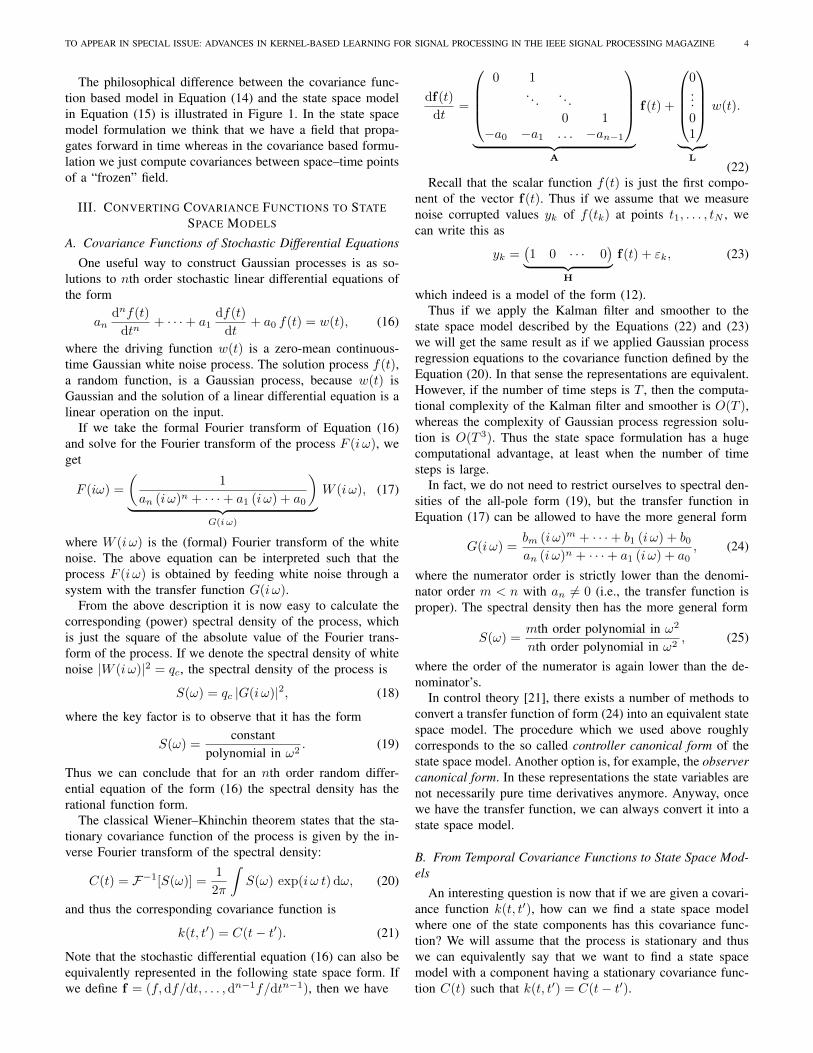
For integer values of p (ν = 1/2, 3/2, . . .), we can expand thisexpression using the binomial formula. For example, if p = 1(ν = 3/2), the corresponding LTI SDE is

df(t)

dt=

(0 1−λ2 −2λ

)f(t) +

(01

)w(t),

where f(t) = (f(t),df(t)/dt). The covariance, spectral den-sity and an example realization are shown in Figure 2.

Example 2 (1D squared exponential covariance function).The one-dimensional squared exponential covariance functionC(τ) = σ2 exp(−τ2/(2l2)) has the spectral density

S(ω) = σ2√

2π l exp

(− l

2 ω2

2

).

This spectral density is not a rational function, but we caneasily approximate it with such a function. By using the Taylorseries of the exponential function we get an approximation

S(ω) ≈ constant1 + l2 ω2 + · · ·+ 1

n! l2n ω2n

which we can factor into stable and unstable parts, and fur-ther convert into an n-dimensional state space model

df(t)

dt= Af(t) + Lw(t).

The covariance, spectral density and a random realization areshown in Figure 2. The error induced by the Taylor series ex-pansion approximation is also illustrated in the figure.

spatial Fourier domain stochastic differential equation whichhas the same temporal spectral density:

an(iωx)∂nf(iωx, t)

∂tn+ · · ·+ a1(iωx)

∂f(iωx, t)

∂t+ a0(iωx) f(iωx, t) = w(iωx, t),

(27)

where the spectral density of the white noise process is somefunction qc(ωx). Analogously to the temporal case (cf. Sec-tion III-A) we can now express this in the following equivalentstate space form:


f(t)

t

Squared exponential

Matern (ν = 3/2)

C(t

−t′)

S(ω

)

Covariance Function Spectral Density−3l 3l 2π−2π

MaternSE (exact)

SE (n = 2)

SE (n = 4)

SE (n = 6)

Fig. 2. Random realizations drawn using the state space models in Exam-ples 1 (green) and 2 (blue). The processes can characterized through their co-variance functions or using their spectral densities. The representation for theMatern covariance function is exact whereas the squared exponential needsto be approximated with a finite-order model (illustrated with n = 2, 4, 6above). The errors in the tails of the spectral density transform into bias atthe origin of the covariance function. With order n = 6, which was alsoused for drawing the random realization, both the approximations are alreadyalmost indistinguishable from the exact ones.

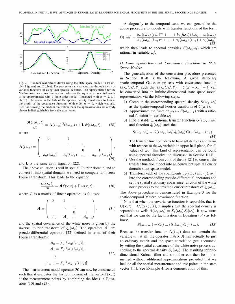
∂ f(iωx, t)

∂t= A(i ωx) f(iωx, t) + L w(iωx, t), (28)

where

A(i ωx) =

0 1

. . . . . .0 1

−a0(iωx) −a1(iωx) . . . −an−1(iωx)

,

(29)and L is the same as in Equation (22).

The above equation is still in spatial Fourier domain and toconvert it into spatial domain, we need to compute its inverseFourier transform. This leads to the equation

∂f(x, t)

∂t= A f(x, t) + Lw(x, t), (30)

where A is a matrix of linear operators as follows:

A =

0 1

. . . . . .0 1

−A0 −A1 . . . −An−1

. (31)

and the spatial covariance of the white noise is given by theinverse Fourier transform of qc(ωx). The operators Aj arepseudo-differential operators [22] defined in terms of theirFourier transforms:

A0 = F−1x [a0(iωx)],

A1 = F−1x [a1(iωx)],

...

An−1 = F−1x [an−1(iωx)].

(32)

The measurement model operator H can now be constructedsuch that it evaluates the first component of the vector f(x, t)at the measurement points by combining the ideas in Equa-tions (10) and (23).

Analogously to the temporal case, we can generalize theabove procedure to models with transfer functions of the form

G(i ωt) =bm(iωx) (i ωt)

m + · · ·+ b1(iωx) (i ωt) + b0(iωx)

an(iωx) (i ωt)n + · · ·+ a1(iωx) (i ωt) + a0(iωx),

(33)which then leads to spectral densities S(ωx, ωt) which arerational in variable ω2

t .

D. From Spatio-Temporal Covariance Functions to StateSpace Models

The generalization of the conversion procedure presentedin Section III-B is the following. A given stationaryspatio-temporal Gaussian process with covariance functionk(x, t;x′, t′) such that k(x, t;x′, t′) = C(x′ − x, t′ − t) canbe converted into an infinite-dimensional state space modelrepresentation via the following steps:

1) Compute the corresponding spectral density S(ωx, ωt)as the spatio-temporal Fourier transform of C(x, t).

2) Approximate the function ωt 7→ S(ωx, ωt) with a ratio-nal function in variable ω2

t .3) Find a stable ωt-rational transfer function G(iωx, i ωt)

and function qc(ωx) such that

S(ωx, ωt) = G(iωx, i ωt) qc(ωx)G(−iωx,−i ωt).(34)

The transfer function needs to have all its roots and zeroswith respect to the ωt variable in upper half plane, for allvalues of ωx. This kind of representation can be foundusing spectral factorization discussed in Section III-B.

4) Use the methods from control theory [21] to convert thetransfer function model into an equivalent spatial Fourierdomain state space model.

5) Transform each of the coefficients aj(iωx) and bj(iωx)into the corresponding pseudo-differential operators andset the spatial stationary covariance function of the whitenoise process to the inverse Fourier transform of qc(ωx).

The above procedure is demonstrated in Example 3 for thespatio-temporal Matern covariance function.

Note that when the covariance function is separable, that is,C(x, t) = Cx(x)Ct(t), it implies that the spectral density isseparable as well: S(ωx, ωt) = Sx(ωx)St(ωt). It now turnsout that we can do the factorization in Equation (34) as fol-lows:

S(ωx, ωt) = G(i ωt)Sx(ωx)G(−i ωt). (35)

Because the transfer function G(i ωt) does not contain thevariable ωx at all, the operator matrix A will actually be justan ordinary matrix and the space correlation gets accountedby setting the spatial covariance of the white noise process ac-cording to the spectral density Sx(ωx). The resulting infinite-dimensional Kalman filter and smoother can then be imple-mented without additional approximations provided that weinclude all the spatial measurement and test points in the statevector [11]. See Example 4 for a demonstration of this.


Example 3 (2D Matern covariance function). The multidi-mensional equivalent of the Matern covariance function givenin Example 1 is the following (r = ‖ξ − ξ′‖, for ξ =(x1, x2, . . . , xd−1, t) ∈ Rd):

C(r) = σ2 21−ν

Γ(ν)

(√2ν

r

l

)νKν

(√2ν

r

l

).

The corresponding spectral density is of the form

S(ωr) = S(ωx, ωt) ∝1

(λ2 + ‖ωx‖2 + ω2t )ν+d/2

.

where λ =√

2ν/l. In order to find the transfer functionG(iωx, iωt), we find the roots of the expression in the denom-inator. They are given by (iωt) = ±

√λ2 − ||iωx||2, which

means we can now extract the transfer function of the stableMarkov process

G(iωx, iωt) =(iωt +

√λ2 − ‖iωx‖2

)−(ν+d/2).

The expansion of the denominator depends on the value ofp = ν + d/2. If p is an integer, the expansion can be easilydone by the binomial theorem. For example, if ν = 1 and d =2, we get the following

∂f(x, t)

∂t=

(0 1

∇2 − λ2 −2√λ2 −∇2

)f(x, t)+

(01

)w(x, t),

(36)where ∇2 is the (spatial) Laplace operator (here the secondpartial derivative w.r.t. x). The one-dimensional example inExample 1 can be seen as a special case of this. An examplerealization of the process is shown in Figure 3.

x

t

Fig. 3: A random realization simulated by the state spacemodel in Equation (36).

E. Non-Causal Stochastic Partial Differential Equations

An important thing to realize is that even if the spatio-temporal covariance function was originally constructed as asolution to some kind of stochastic partial differential equa-tion, we might still need to do the above factorization. Forexample, consider the following stochastic partial differentialequation (SPDE) due to Whittle [23]:

∂2f(x, t)

∂x2+∂2f(x, t)

∂t2− λ2 f(x, t) = w(x, t), (37)

where w(x, t) is a space–time white Gaussian random field.Fourier transforming the system and computing the spectraldensity gives the stationary covariance function

C(x, t) =

√x2 + t2

2λK1(λ

√x2 + t2), (38)

Example 4 (2D squared exponential covariance function). Thesquared exponential covariance function

k(x, t;x′, t′) = σ2 exp(−α‖x− x′‖2 − α|t− t′|2),

where α = 1/(2l2), is separable, which means that its spectraldensity

S(ωx, ωt) =(πα

)d/2exp

(−‖ωx‖

2

4α

)exp

(−ω

2t

4α

)is also separable. We use the truncated series approximationto the temporal part from Example 2, which leaves us with anapproximation S(ωx, ωt) ≈ |G(i ωt)|2Sw(ωx). If we definef(x, t) = (f(x, t), ∂f(x, t)/∂t, . . . , ∂n−1f(x, t)/∂tn−1), col-lecting the terms from the transfer function gives the solution

∂f(x, t)

∂t= Af(x, t) + Lw(x, t),

where w(x, t) is a time-white process with a spatial spectraldensity Sw(ωx) and the matrix A is the same as in Exam-ple 2. Because A does not contain any operators, the corre-sponding infinite-dimensional Kalman filter and smoother canbe implemented without any additional approximations.

which can be seen as a special case of the covariance functionin Example 3. But if we converted the SPDE in Equation (37)into a state space model, we would get a different state spacemodel than in Equation (36) and the model would not evencontain pseudo-differential operators at all. Now the catch isthat if we did that, the resulting model would not be a stablesystem. This is because the Equation (37) corresponds to se-lection of the roots of the spectral density in such way that allof them are not in the upper half of the complex plane. Thusthe process is not Markovian.

IV. INFINITE-DIMENSIONAL BAYESIAN FILTERING,SMOOTHING AND PARAMETER ESTIMATION

A. Infinite-Dimensional Kalman Filtering and Smoothing ofSpatio-Temporal Gaussian Processes

Using the procedure outlined in the previous section we canconvert given stationary spatio-temporal covariance functionsinto equivalent infinite-dimensional state space models. Thespatio-temporal Gaussian process regression solution can bethen computed with the infinite-dimensional Kalman filter andsmoother [18], [11].

However, in practice, we cannot implement the infinite-dimensional Kalman filters and smoothers exactly, but thepseudo-differential operator equations appearing in the equa-tions need to be solved numerically. Fortunately, we can usethe wide arsenal of numerical methods developed for determin-istic pseudo-differential and partial differential equation mod-els for that purpose. Because stationary covariance functionmodels always lead to equations, which can be expressed interms of the Laplace operator, a particularly useful method isto approximate the solution using the eigenbasis of the Laplaceoperator [11], [24].


12 24 36 48 60 72 84 96 108 1200

100

200

300

Time (months)

Pre

cip

ita

tio

n (

mm

)

True

Estimate

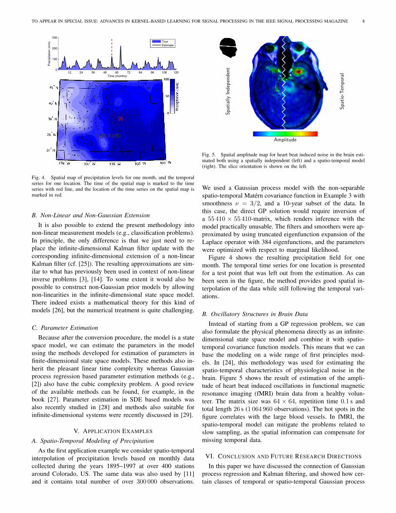
Fig. 4. Spatial map of precipitation levels for one month, and the temporalseries for one location. The time of the spatial map is marked to the timeseries with red line, and the location of the time series on the spatial map ismarked in red.

B. Non-Linear and Non-Gaussian Extension

It is also possible to extend the present methodology intonon-linear measurement models (e.g., classification problems).In principle, the only difference is that we just need to re-place the infinite-dimensional Kalman filter update with thecorresponding infinite-dimensional extension of a non-linearKalman filter (cf. [25]). The resulting approximations are sim-ilar to what has previously been used in context of non-linearinverse problems [3], [14]. To some extent it would also bepossible to construct non-Gaussian prior models by allowingnon-linearities in the infinite-dimensional state space model.There indeed exists a mathematical theory for this kind ofmodels [26], but the numerical treatment is quite challenging.

C. Parameter Estimation

Because after the conversion procedure, the model is a statespace model, we can estimate the parameters in the modelusing the methods developed for estimation of parameters infinite-dimensional state space models. These methods also in-herit the pleasant linear time complexity whereas Gaussianprocess regression based parameter estimation methods (e.g.,[2]) also have the cubic complexity problem. A good reviewof the available methods can be found, for example, in thebook [27]. Parameter estimation in SDE based models wasalso recently studied in [28] and methods also suitable forinfinite-dimensional systems were recently discussed in [29].

V. APPLICATION EXAMPLES

A. Spatio-Temporal Modeling of Precipitation

As the first application example we consider spatio-temporalinterpolation of precipitation levels based on monthly datacollected during the years 1895–1997 at over 400 stationsaround Colorado, US. The same data was also used by [11]and it contains total number of over 300 000 observations.

Spatio-Tem

poral

Spatially

Independent

Amplitude

Fig. 5. Spatial amplitude map for heart beat induced noise in the brain esti-mated both using a spatially independent (left) and a spatio-temporal model(right). The slice orientation is shown on the left.

We used a Gaussian process model with the non-separablespatio-temporal Matern covariance function in Example 3 withsmoothness ν = 3/2, and a 10-year subset of the data. Inthis case, the direct GP solution would require inversion ofa 55 410 × 55 410-matrix, which renders inference with themodel practically unusable. The filters and smoothers were ap-proximated by using truncated eigenfunction expansion of theLaplace operator with 384 eigenfunctions, and the parameterswere optimized with respect to marginal likelihood.

Figure 4 shows the resulting precipitation field for onemonth. The temporal time series for one location is presentedfor a test point that was left out from the estimation. As canbeen seen in the figure, the method provides good spatial in-terpolation of the data while still following the temporal vari-ations.

B. Oscillatory Structures in Brain Data

Instead of starting from a GP regression problem, we canalso formulate the physical phenomena directly as an infinite-dimensional state space model and combine it with spatio-temporal covariance function models. This means that we canbase the modeling on a wide range of first principles mod-els. In [24], this methodology was used for estimating thespatio-temporal characteristics of physiological noise in thebrain. Figure 5 shows the result of estimation of the ampli-tude of heart beat induced oscillations in functional magneticresonance imaging (fMRI) brain data from a healthy volun-teer. The matrix size was 64 × 64, repetition time 0.1 s andtotal length 26 s (1 064 960 observations). The hot spots in thefigure correlates with the large blood vessels. In fMRI, thespatio-temporal model can mitigate the problems related toslow sampling, as the spatial information can compensate formissing temporal data.

VI. CONCLUSION AND FUTURE RESEARCH DIRECTIONS

In this paper we have discussed the connection of Gaussianprocess regression and Kalman filtering, and showed how cer-tain classes of temporal or spatio-temporal Gaussian process


regression problems can be converted into finite or infinite-dimensional state space models. The advantage of this for-mulation is that it allows the use of computationally efficientlinear-time-complexity Kalman filtering and smoothing meth-ods. This type of methods are particularly important in signalprocessing, because there the interest lies in processing long(unbounded) time series and thus it is necessary to have linearcomplexity in time.

One limitation in the present methodology is that it can onlybe used with stationary covariance functions. This arises fromthe use of Fourier transform which only works with station-ary systems. In practice, this is not so huge a restriction, be-cause stationary covariance functions are the most commonlyused class of covariance functions in machine learning andspatial statistics [2], [1]. Non-stationary processes could beconstructed, for example, by changing the stationary opera-tors or covariance functions in the state space model into non-stationary ones, by embedding the stationary model inside anon-stationary partial differential equation, or by changing thecoordinate system of the input space suitably (cf. [12]).

Although the present method solves the problem of temporaltime complexity, the space complexity is still cubic in the num-ber of measurements. Fortunately, it is also possible to com-bine the present methods with computationally efficient sparseapproximations [19], [2]. These methods are also closely re-lated to basis function expansion methods (cf. [11], [24]). FastFourier Transform (FFT) can also be used for speeding upthe computations in applications such as computer vision andbrain imaging.

REFERENCES

[1] A. E. Gelfand, P. J. Diggle, Montserrat, and P. Guttorp, Handbook ofSpatial Statistics. CRC Press, 2010.

[2] C. E. Rasmussen and C. K. I. Williams, Gaussian Processes for MachineLearning. MIT Press, 2006.

[3] A. Tarantola, Inverse Problem Theory and Methods for Model ParameterEstimation. SIAM, 2004.

[4] J. Kaipio and E. Somersalo, Statistical and Computational Inverse Prob-lems. Springer, 2005.

[5] M. S. Grewal and A. P. Andrews, Kalman Filtering, Theory and PracticeUsing MATLAB. Wiley Interscience, 2001.

[6] G. Wahba, Spline Models for Observational Data. SIAM, 1990.[7] B. Øksendal, Stochastic Differential Equations: An Introduction with

Applications, 6th ed. Springer, 2003.[8] M. Alvarez and N. D. Lawrence, “Latent force models,” in JMLR Work-

shop and Conference Proceedings Volume 5 (AISTATS 2009), 2009, pp.9–16.

[9] J. Hartikainen, M. Seppanen, and S. Sarkka, “State-space inference fornon-linear latent force models with application to satellite orbit predic-tion,” in Proceedings of The 29th International Conference on MachineLearning (ICML 2012), 2012.

[10] J. Hartikainen and S. Sarkka, “Kalman filtering and smoothing solu-tions to temporal Gaussian process regression models,” in Proceedingsof IEEE International Workshop on Machine Learning for Signal Pro-cessing (MLSP), 2010.

[11] S. Sarkka and J. Hartikainen, “Infinite-dimensional Kalman filtering ap-proach to spatio-temporal Gaussian process regression,” in JMLR Work-shop and Conference Proceedings Volume 22 (AISTATS 2012), 2012,pp. 993–1001.

[12] F. Lindgren, H. Rue, and J. Lindstrom, “An explicit link between Gaus-sian fields and Gaussian Markov random fields: the stochastic partialdifferential equation approach,” Journal of the Royal Statistical Society:Series B (Statistical Methodology), vol. 73, no. 4, pp. 423–498, 2011.

[13] N. Cressie and C. K. Wikle, “Space-time Kalman filter,” in Encyclope-dia of Environmetrics, A. H. El-Shaarawi and W. W. Piegorsch, Eds.John Wiley & Sons, Ltd, Chichester, 2002, vol. 4, pp. 2045–2049.

[14] P. Hiltunen, S. Sarkka, I. Nissila, A. Lajunen, and J. Lampinen, “Statespace regularization in the nonstationary inverse problem for diffuse op-tical tomography,” Inverse Problems, vol. 27, p. 025009, 2011.

[15] L. Csato and M. Opper, “Sparse on-line Gaussian processes,” NeuralComputation, vol. 14, no. 3, pp. 641–668, 2002.

[16] W. Liu, I. Park, Y. Wang, and J. Prıncipe, “Extended kernel recur-sive least squares algorithm,” IEEE Transactions on Signal Processing,vol. 57, no. 10, pp. 3801–3814, 2009.

[17] S. Van Vaerenbergh, M. Lazaro-Gredilla, and I. Santamarıa, “Kernel re-cursive least-squares tracker for time-varying regression,” IEEE Trans-actions on Neural Networks and Learning Systems, vol. 23, no. 8, pp.1313–1326, 2012.

[18] R. Curtain, “A survey of infinite-dimensional filtering,” SIAM Review,vol. 17, no. 3, pp. 395–411, 1975.

[19] J. Quinonero-Candela and C. E. Rasmussen, “A unifying view of sparseapproximate Gaussian process regression,” JMLR, vol. 6, pp. 1939–1959,2005.

[20] S. Sarkka, “Linear operators and stochastic partial differential equationsin Gaussian process regression,” in Lecture Notes in Computer ScienceVolume 6792 (ICANN 2011), 2011, pp. 151–158.

[21] T. Glad and L. Ljung, Control Theory: Multivariable and NonlinearMethods. Taylor & Francis, 2000.

[22] M. A. Shubin, Pseudodifferential operators and spectral theory.Springer-Verlag, 1987.

[23] P. Whittle, “On stationary processes in the plane,” Biometrica, vol. 41,no. 3/4, pp. 434–449, 1954.

[24] A. Solin, “Hilbert space methods in infinite-dimensional Kalman filter-ing,” Master’s thesis, Aalto University, 2012.

[25] S. Sarkka and J. Sarmavuori, “Gaussian filtering and smoothing forcontinuous-discrete dynamic systems,” Signal Processing, vol. 93, no. 2,pp. 500–510, 2013.

[26] G. Da Prato and J. Zabczyk, Stochastic Equations in Infinite Dimensions.Cambridge University Press, 1992.

[27] O. Cappe, E. Eric Moulines, and T. Ryden, Inference in hidden Markovmodels. Springer, 2005.

[28] I. S. Mbalawata, S. Sarkka, and H. Haario, “Parameter estimation instochastic differential equations with Markov chain Monte Carlo andnon-linear Kalman filtering,” Computational Statistics, 2013, (in press).

[29] H. Singer, “Continuous-discrete state-space modeling of panel datawith nonlinear filter algorithms,” AStA Advances in Statistical Analysis,vol. 95, no. 4, pp. 375–413, 2011.

Documents

TO APPEAR IN SPECIAL ISSUE: ADVANCES IN …becs.aalto.fi/~ssarkka/pub/inf-bayes-draft.pdfTO APPEAR IN SPECIAL ISSUE: ADVANCES IN KERNEL-BASED LEARNING FOR SIGNAL PROCESSING IN THE