Embed Size (px)
Citation preview

Earth, Life & Social Sciences
Van Mourik Broekmanweg 6
2628 XE Delft
Postbus 49
2600 AA Delft
www.tno.nl
T +31 88 866 30 00
F +31 88 866 30 10
TNO-rapport
TNO 2015 R10955
Correction algorithms for WLTP chassis
dynamometer and coast-down testing
Datum 9 July 2015
Auteur(s) Norbert E. Ligterink
Pim van Mensch
Rob F.A. Cuelenaere
Stefan Hausberger
David Leitner
Gérard Silberholz
Exemplaarnummer 2016-TL-RAP-0100293115
Aantal pagina's 120 (incl. bijlagen)
Aantal bijlagen 7
Opdrachtgever European Commission, DG Clima
Franework Contract ENTR/F1/2009/030 – Lot 4
Projectnaam WLTP correction algorithms
Projectnummer 060.03678
Alle rechten voorbehouden.
Niets uit deze uitgave mag worden vermenigvuldigd en/of openbaar gemaakt door middel
van druk, foto-kopie, microfilm of op welke andere wijze dan ook, zonder voorafgaande
toestemming van TNO.
Indien dit rapport in opdracht werd uitgebracht, wordt voor de rechten en verplichtingen van
opdrachtgever en opdrachtnemer verwezen naar de Algemene Voorwaarden voor
opdrachten aan TNO, dan wel de betreffende terzake tussen de partijen gesloten
overeenkomst.
Het ter inzage geven van het TNO-rapport aan direct belang-hebbenden is toegestaan.
© 2015 TNO

TNO-rapport | TNO 2015 R10955 | 9 July 2015 2 / 73
Table of contents
Summary .................................................................................................................. 5
1 Introduction ............................................................................................................ 16
Chassis dynamometer testing ................................................................................. 17 1.1
The physical principles of coast down testing ......................................................... 18 1.2
2 Correction algorithms for chassis dynamometer tests in WLTP ..................... 20
Calculation of the vehicle specific Veline equation .................................................. 20 2.1
Deviation against target speed ................................................................................ 22 2.2
Quality of reference fuel .......................................................................................... 25 2.3
Inlet air temperature and humidity ........................................................................... 29 2.4
Battery state of charge............................................................................................. 32 2.5
Temperatures from preconditioning and soak ......................................................... 35 2.6
Inaccuracy of road load setting ................................................................................ 39 2.7
Electrified vehicles ................................................................................................... 43 2.8
Gear shifts ............................................................................................................... 43 2.9
Accuracy of relevant sensor signals for correction functions .................................. 46 2.10
3 WLTP coast-down test procedure ....................................................................... 48
Corrections included in the WLTP ........................................................................... 48 3.1
Vehicle preparation .................................................................................................. 52 3.2
Vehicle conditioning ................................................................................................. 53 3.3
Coast-down test ....................................................................................................... 53 3.4
4 Ambient conditions ............................................................................................... 56
Weather ................................................................................................................... 56 4.1
Wind ......................................................................................................................... 59 4.2
Test track ................................................................................................................. 61 4.3
5 Inertia ...................................................................................................................... 64
Vehicle weight .......................................................................................................... 64 5.1
Weight balance only has a minor influence on coast-down and therefore it has not 5.2
been considered for further analysis.”Rotating inertia ............................................. 65
6 Rolling resistance .................................................................................................. 68
Tyre .......................................................................................................................... 68 6.1
Drive line resistance ................................................................................................ 69 6.2
7 Air-drag ................................................................................................................... 71

TNO-rapport | TNO 2015 R10955 | 9 July 2015 3 / 73
Vehicle model variations .......................................................................................... 71 7.1
8 Literature ................................................................................................................ 73
9 Signature ................................................................................................................ 74
Bijlage(n)
A. Abbrevations
B. Standard conditions
C. Application of the correction methods on chassis dyno tests
c.1 TUG vehicle
c.2 JRC vehicle
c.3 JARI vehicle
D. Coast down formulae
d.1 Coast down curve
d.2 F1=0 approximation
E. Coast down validation
e.1 WLTP corrections
e.2 Consistent effects as observed
F. Coast down test program
f.1 Background
f.2 Aim and approach
f.3 Structure of this appendix
f.4 Test vehicle
f.5 Test tracks
f.6 Test equipment
f.7 Test procedure
f.8 Coast-down measurement program
f.9 Reference situation
f.10 Rolling resistance and inertia
f.11 Alternative wheel alignment
f.12 Test mass high and extra low
f.13 Air resistance
f.14 Ambient conditions and road properties
G. Suggested WLTP gtr amendments for deviation against target speed and
road load calibration

TNO-rapport | TNO 2015 R10955 | 9 July 2015 4 / 73
g.1 Amendments describing the correction for deviations against the
target speed
g.2 Amendments in the definition of road load calibration on the chassis
dynamometer

TNO-rapport | TNO 2015 R10955 | 9 July 2015 5 / 73
Summary
The flexibilities allowed in the WLTP are necessary to allow efficient testing without
having a lot of invalid tests. Nevertheless some of the flexibilities can influence the
resulting fuel consumption to an extent which makes it worth considering the
application of correction functions to compensate for deviations against the target
values. Such correction functions have several benefits:
+ The repeatability increases
+ In test programs other than type approval tests, larger deviations against the
target values may be typical. In such cases the application of the correction
functions could help to make single tests better comparable and to increase the
repeatability.
+ Making use of the flexibilities to reduce the CO2 test result gives a better type
approval value but does not influence the real world CO2 emissions. Thus the
test result should reflect reality better if the result is corrected for deviations
against the target values of the test procedure.
+ The need to optimise the position of the test conditions within the range of
flexibilities is reduced to a large extent. Making use of flexibilities ranges from
driver training over calibration of test utilities up to optimising the alternator
control unit to cycle conditions. Eliminating the need for optimisation of such
parameters shall reduce the overall effort for testing without negative effect on
real world CO2 emissions.
- A negative impact is that the complexity of the test evaluation increases and additional signals need to be measured, such as current flow to and from the battery.
The report investigates a series of corrections that could be applied to variations of
test parameters within the tolerances ranges allowed by the WLTP GTR provisions.
The corrections cover both the chassis dynamometer and coast down test
procedure.
The proposed corrections have been discussed with stakeholders on numerous
occasions, particularly in the WLTP Informal Working Group (IWG)1 and the
Working Party on Pollution and Energy (GRPE)2 both residing under the United
Nations in Geneva. Several of the proposed corrections have already been adopted
by the WLTP Informal Working Group and will be implemented in the WLTP global
technical regulation phase 1b, scheduled for publication in 2016. Some proposals
were rejected by the WLTP IWG and GRPE and the Commission Services decided
not to proceed with these proposals. Other proposals are suited for introduction as
part of the EU implementation of the WLTP. These proposals will be further
developed outside the scope of this project.
The following table provides an overview for the further proceedings with respect to
the individual cycle tolerances investigated in the report. The numbers refer to the
paragraphs in the main report.
1 https://www2.unece.org/wiki/display/trans/WLTP+8th+session
2 http://www.unece.org/trans/main/wp29/wp29wgs/wp29grpe/grpeinf69.html

TNO-rapport | TNO 2015 R10955 | 9 July 2015 6 / 73
Correction type Progress
2.2 Deviation against target
speed
The method for addressing the issue is fully developed in the
report, relevant impact on CO2 emissions of up to 5%.
Deviation against target speed will be a WLTP Phase 2 working
item.
2.3 Quality of reference fuel Impact on CO2 emissions still to be investigated outside
timeframe of this project.
2.4 Inlet air temperature and
humidity
Impact on CO2 emissions found by simulation is low. In contrary
measurements on one vehicle shows influence up to 2%.
Influences from ECU controllers and from physical effects are
unclear yet.
2.5 Battery state of charge
correction
Battery SOC correction is already included in WLTP Phase 1.
The significant impact on CO2 emissions (of up to 3%) is
confirmed.
2.6 Temperature from
preconditioning and soak
Very small impact on CO2 emissions (< 0,4%)
2.7 Inaccuracy of road load
setting on the chassis
dynamometer
Several options for addressing the issue are available,
relevant impact on CO2 emissions of up to 3%.
Proposal on time between warm-up and testing adopted for
WLTP Phase 1b.
2.9 Deviation from designated
gear shift points
There seems to be a relevant influence on CO2 emissions,
however there are no ideas yet how the issue could be
addressed as long as gear shifts are not recorded in the test.
3.2 Vehicle preparation for
coast down: toe-in prescription
There is a relevant influence of the wheel alignment on road
load coefficients.
Proposal adopted for WLTP Phase 1b.
3.3 Vehicle conditioning for
coast down: tyre pressure
monitoring/control
There is a relevant influence of the tyre pressure on road load
coefficients, the requirements suggested are not so
straightforward to implement. Concrete proposal available.
4.1 Ambient weather conditions
at coast down: temperature, air
pressure, water content of the
air
There is a relevant influence of these parameters on the air
drag measured at coast downs. In the current WLTP GTR there
is already a correction for the air density, but a concrete
proposal for relative humidity is available.
4.2 Wind corrections at coast
down
Albeit the current WLTP GTR already contains a wind correction
further restrictions on side wind and gustiness may be

TNO-rapport | TNO 2015 R10955 | 9 July 2015 7 / 73
necessary. A concrete proposal for gustiness is available
4.3 Road condition of coast
down test track (surface
roughness, gradient,
undulation)
The road surface of the test track seems to have a significant
influence. It should therefore be envisaged to either require a
minimum road "roughness" or to correct road loads measured
at a given test track against a "standard" road surface.
However, the investigation of relevant roughness parameters
and "standard" road surface values is quite complex. Outside
timeframe of this project.
5.2 Rotational inertia correction
(when evaluating the coast
down test)
The suggested correction is very simple to implement and
provides a more accurate result for CO2 emissions.
6.1 Tyre rolling resistance The rolling resistance of the test tyre might deviate from the
class value. The suggested correction is very simple to
implement and provides a more accurate result for CO2
emissions, but depends on the availability of the actual rolling
resistance value of the test tyre. Outside timeframe of this
project.
7.1 Movable body parts, in
particular grill vanes
Positions of movable body parts, in particular grill vanes, have a
significant influence on the vehicle air drag. Their position
during coast down might deviate from the position in normal
use. The suggested correction is very simple to implement.
The correction methods are summarised below. A detailed description of the
methods and test results is provided in the main report.
Correction algorithms for chassis dynamometer tests in WLTP
Correction methods for several flexibilities existing in chassis dynamometer tests
have been elaborated and the influence on the resulting CO2 emissions has been
assessed where possible. For the corrections which have reasonable influence on
the results and which are already developed to an applicable draft procedure the
amendments in the WLTP necessary for their implementation are drafted in Annex
G. These are:
- A draft for the amendments to implement a correction for deviations against
the target velocity and the target test distance (Annex G.1).
- A draft for the amendments to define the procedure for adjustments in the
road load more precisely (Annex G.2).
All flexibilities analysed are summarised below. More detailed information is given
for each correction function in the corresponding chapters of the report.
Vehicle specific CO2 linear equation (“Veline”): Several of the correction functions
need to adapt the measured CO2 value from the work delivered during the test to
the target work which would have been necessary without flexibilities. These
corrections need a specific CO2 emission coefficient in [g/kWh]. This coefficient is
not based on the average engine efficiency in the test cycle but represents the

TNO-rapport | TNO 2015 R10955 | 9 July 2015 8 / 73
additional fuel flow (CO2 emissions) due to an additional engine power demand.
Thus in this coefficient those parasitic losses which are not affected by changes in
engine power are not considered, since these have to be overcome in any case.
This emission coefficient is called in this report the “Veline coefficient”. It can be
computed from the chassis dynamometer tests from the four phases of the WLTC
by plotting the average CO2 flow [g/s] over the average power of the phase as
shown in Figure 1. The regression line gives the “Veline equation”, where the
inclination coefficient “k” of the equation gives the average Veline coefficient. In the
equation the parasitic losses are represented by the constant “D” in the equation,
which gives the CO2 emissions (or the fuel consumption (FC), if FC is plotted
instead of CO2) at zero power output3.
Figure 1: Schematic picture of setting up the Veline for a LDV from the chassis dyno test
The Veline equation gives the CO2 flow as a function of the power at the wheel. The
Veline coefficient from this equation is suitable to correct all parameters leading to
deviations of the work at the wheel against target settings (results from speed
deviations and from road load settings)4. To gain the engine Willans coefficient
5 the
Veline coefficient would have to be translated to the engine power, which is higher
than the wheel power due to the losses in the transmission system in case of
positive power output. The losses in the transmission system are not measured in
the test and each WLTC phase has different engine speed levels. Thus the engine
Willans lines cannot be computed exactly from the Velines and a conversion would
add reasonable uncertainties to the engine Willans coefficient. Therefore it seems
to be more practical to use directly generic engine Willans coefficients for all
3 Typically the regression line of the average engine speed per WLTC phase over average power
crosses the zero power line at engine speeds clearly above idling speed. Thus the constant value
“D” in the linear equation represents the CO2 emission value for idling at increased rpm.
4 All corrections based on the Veline coefficients [g/kWh] can either be based on the change in
power to provide the average change in fuel flow [g/s] or by change in work over the cycle to
provide the absolute change in fuel consumption over the cycle [g]. Both methods deliver identical
results.
5 The engine Willans lines are defined as functions providing the fuel flow or CO2 emissions of the
engine as function of the engine power at constant engine speed values.

TNO-rapport | TNO 2015 R10955 | 9 July 2015 9 / 73
corrections which are based on deviations of the engine power over the cycle. This
option is already applied in the actual WLTP for correction of SOC imbalances of
the battery.
Below an overview on potential correction functions is given which partially make
use of the vehicle specific Veline or the generic engine related Willans coefficient.
Imbalance in battery SOC can influence the test result up to approx. 2 g/km in the
WLTC. A correction for SOC imbalances is suggested to be based on generic
coefficients for the change in fuel flow per change in average power demand over
the cycle (“engine Willans coefficient”) combined with a generic average alternator
efficiency as already outlined in the WLTP. More detailed approaches have been
investigated at TUG but do not show significant improvements in the reliability of the
correction (Leitner, 2014). This gives the following equation for the suggested
correction:
𝑊𝑏𝑎𝑡 = ∫ 𝑈(𝑡) ∗ 𝐼(𝑡) ∗ 0.001 𝑑𝑡 in [kWs] where the Voltage could be the
nominal Voltage or the measured one. The Current flow has to be measured at the battery with positive sign for energy flows from the battery.
∆CO2SOC [g]=
Wbat
*ke
With ke ........... Engine Willans coefficient [gCO2/kWs], generic values per
technology
............ Generic average efficiency of the alternator including
transmission losses to the engine (in the WLTP draft an
efficiency of 0.67 is suggested)
The correction shall be done for each WLTC phase separately, if a more accurate
base shall be provided for setting up the vehicle specific Veline functions from the
SOC corrected WLTP results. This is more relevant, if the test is started with low
SOC since the vehicle then tends to load the battery from start on, which influences
mainly the first test phase. In type approval the defined pre-conditioning and the
limits for the SOC imbalance should allow only small influences on the CO2
emissions per test phase. Thus the SOC correction may be applied to the entire
WLTC and not per phase.
Deviation against target road load: As the basis for a correction, a set of 3 coast
down tests6 shall be performed directly after the WLTC. The tests with the highest
and the shortest coast down time shall be rejected and the remaining test shall be
evaluated according to the WLTP regulation7 to determine the road load
coefficients. Forthe time being it is assumed that the coast down after the WLTC
test shall be representative for the road loads applied by the chassis dynamometer
during the test. The correction can be done separately or preferably should be
combined with the correction for deviations against the target speed.
6 The exact number may need further discussion. Alternatively just one test after WLTC can be
made, if we do not expect outliers, see chapter 2.7.
7 for the coast down test evaluation on the test track

TNO-rapport | TNO 2015 R10955 | 9 July 2015 10 / 73
A separate correction for the road load would work as follows:
The actual wheel power for the road load coefficients from the chassis dyno coast
down test has to be calculated from the vehicle speed and acceleration and has to
be compared against the wheel power from the target road load values.
The time resolution of the speed signal shall be at minimum 5 Hz. The velocity and
acceleration shall be calculated as follows:
a(j) = ( v(i+1) – v(i) ) / (t(i+1) – t(i) )
v(j) = ( v(i+1) + v(i) ) * 0.5 (velocity measured in the WLTC)
with i ................ original reading of the velocity in >5Hz
j ................ transformed time steps
The instantaneous power is calculated from the measured road load coefficients as
follows:
P(j) = (R0 + R1*v(j) +R2*v(j) ² + m*a(j)) * v(j)
The instantaneous power is calculated from the target road load coefficients as
follows:
Pp(j) = (R0w + R1w*v(j) +R2w*v(j) ² + m*a(j)) * v(j)
with R0, R1 R2 .............. Road load from the coast down tests at the chassis
dyno directly after the WLTC in [N], [N*s/m] and [N*s²/m²]
R0w, R1w R2w ............................. Target road load coefficients in [N], [N*s/m] and
[N*s²/m²]
Then the average power values over the WLTC are computed
P̅ =∑ 𝑃(𝑗)𝑛
𝑗=1
𝑛
P�̅� =∑ 𝑃𝑝(𝑗)𝑛
𝑗=1
𝑛
with n............... number of time steps in the WLTC recording
Consequently the total work at wheels is calculated:
∆𝑊𝑤ℎ𝑒𝑒𝑙 = 1.8 × (�̅�𝑝 − �̅�) in [kWs]
Then the vehicle based Veline function is applied to correct for the deviation against
the work from the WLTC target velocity:
∆𝑪𝑶𝟐𝒑 [𝒈] = ∆𝑾𝒘𝒉𝒆𝒆𝒍 ∗ 𝒌𝒗
with kv ................ Vehicle Veline coefficient [gCO2/kWs] from WLTP
If the road load correction is applied it is suggested to combine it with the correction
for target speed deviations as described later in this summary.
Remark: The coast-down tests after the WLTC are assumed to have a similar
uncertainty in representing the road load during the test as the coast downs during
the chassis dynamometer calibration procedure. Thus instead of correcting for
deviations in the road load as described above, a more precise procedure for the
chassis dynamometer road load calibration could be applied. If the tolerances in the
road load simulated are low, the correction is assumed not to be necessary since
then the effect of the correction would be very small. For both options it is essential

TNO-rapport | TNO 2015 R10955 | 9 July 2015 11 / 73
that the number of coast down tests as well as the space of time between vehicle
driving and each subsequent coast down test is defined in detail. Otherwise the
temperatures of tyres and bearings will change (drop over time) and lead to
different road load values than those in the test procedure. For a precisely defined
procedure for the chassis dynamometer road load calibration the total number of
coast downs shall be defined exactly and also the space of time between the coast
downs has to be defined (suggested that this be amended in Annex 4 in WLTP, e.g.
para 8.1.3.2.1). For calibration of the road load settings, a maximum number of 5
coast down seems to be reasonable, with a maximum of 3 minutes between the
vehicle warm and the first coast down and also a maximum of 3 minutes between
the end of a coast down and the start of the subsequent coast down.
Deviation against target speed: the driven speed profile as well as for the target
speed the power at wheels is computed. If combined with the correction for road
load deviations, the power for the speed driven in the WLTC is calculated from the
road load coefficients gained from the coast down after the WLTC test as described
above:
P(j) = (R0 + R1*v(j)+R2*v(j)² + m*a(j)) * v(j) where v(j) is the
velocity driven in
[m/s]
Pw(t) = (R0-w + R1-w*vw(j)+R2-w*vw(j)² + m*aw(j)) * vw(j) where vw is the
target velocity of
the WLTC
As described for the road load correction, the time resolution of the speed signal
shall be at minimum 5 Hz. The velocity and acceleration shall be calculated as
described before.
Then the difference in the average of the power signals above Poverrun is calculated.
if P(j) < 𝑃𝑜𝑣𝑒𝑟𝑟𝑢𝑛 then P(j) = 𝑃𝑜𝑣𝑒𝑟𝑟𝑢𝑛
if P𝑊(j) < 𝑃𝑜𝑣𝑒𝑟𝑟𝑢𝑛 then P𝑊(j) = 𝑃𝑜𝑣𝑒𝑟𝑟𝑢𝑛
P̅ =∑ 𝑃(𝑗)𝑛
𝑗=1
𝑛
P𝑊̅̅̅̅ =
∑ 𝑃(𝑗)𝑛𝑗=1
𝑛
with n............... number of transformed time steps (n = i–1)
The deviation against the target cycle work is then:
∆𝑊𝑤ℎ𝑒𝑒𝑙 = 1.8 × (�̅�𝑤 − �̅�) in [kWs]
Then the vehicle based Veline function is applied to correct for deviations against
the work from the WLTC target velocity
∆𝐶𝑂2𝑣 [𝑔] = ∆𝑊𝑤ℎ𝑒𝑒𝑙 ∗ 𝑘𝑣
With kv ................ Vehicle Veline coefficient [gCO2/kWs] from WLTP result
after SOC correction
The correction for deviations against target speed covers the time shares in WLTP
with wheel power above “Poverrun”, as shown in Figure 1. Thus in these time intervals
the power is shifted to the power necessary to meet the target velocity.

TNO-rapport | TNO 2015 R10955 | 9 July 2015 12 / 73
Nevertheless, by braking less or more aggressively than the target decelerations,
the distance can be varied by the driver with only small effects on the total WLTC
fuel consumption [g], since in these phases the engine is generally in overrun at
zero fuel flow. Thus dividing the entire fuel consumption in the test (in [g]) by the
target distance of the WLTC gives a result without effects from braking behaviour of
the driver:
𝑪𝑶𝟐[𝒈/𝒌𝒎] = 𝑪𝑶𝟐𝒎𝒆𝒂𝒔𝒖𝒓𝒆𝒅
+ ∆𝑪𝑶𝟐𝑺𝑶𝑪+ ∆𝑪𝑶𝟐𝒗
𝟐𝟑. 𝟐𝟕
With CO2measured .......... CO2 test result in the WLTP in [g/test]
23.27 .................. WLT target test distance [km]
The driver can influence the resulting CO2 emissions in the WLTC by more than 2%
within the given speed tolerances. Thus a correction for deviations against the
target speed is suggested to improve the repeatability and the reproducibility of test
results.
Deviation against target soak temperature: the WLTP prescribes a soak
temperature of 23°C +3°C. These rather narrow tolerances will not lead to
deviations in the CO2 emissions measured of more than approx. + 0.6%. If the oil
temperature at test start is measured with reasonable accuracy a correction of this
influence may be reasonable.
A linear equation for the small temperature range seems to be the best option:
∆𝑪𝑶𝟐𝒕 = (𝟐𝟑 − 𝐭) ∗ 𝑪𝑻
With: CT ............... Coefficient for soak temperature correction (average from
measurements: CT- = 0.0018/°C)
𝐶𝑂2 [𝑔
𝑘𝑚] = 𝐶𝑂2𝑚𝑒𝑎𝑠𝑢𝑟𝑒𝑑 [
𝑔
𝑘𝑚] × (1 + ∆𝐶𝑂2)
An accurate assessment of the oil temperature would need an additional sensor in
the test procedure, a precise definition of a representative point of measurement
and a definition of the accuracy of the temperature sensors. Since the effect of the
temperature correction is rather small a mandatory correction of the soak
temperature seems not to be very attractive.
The order of correction steps is outlined below as a suggestion from TUG. Which
corrections shall be implemented in type approval needs further discussion in the
relevant expert groups. The main questions are whether the effort is balanced with
the improvement in accuracy and whether the quality of input data is sufficient to
apply the correction8.
1) Perform the WLTP test
Measured values necessary for application of the correction functions: CO2 [g],
distance [km], SOC [kWh], instantaneous velocity with > 5 Hz [km/h] to compute
average Pwheel [kW] per phase.
8 the accuracy of the sensor signals should be approx. an order of magnitude higher than the
tolerances which shall be corrected (e.g. < +0.2°C sensor accuracy for a correction of +3°C; to be
discussed.

TNO-rapport | TNO 2015 R10955 | 9 July 2015 13 / 73
For application of the correction for road load deviations also a set of 3 coast down
tests directly after the WLTC would be required.
2) Correct test results for imbalances in battery SOC
3) Set up a vehicle specific Veline function from the SOC-corrected WLTC test data
4) Optional: Correct for deviation against target road load settings (can be
combined with 5)) or use a more precise definition in the WLTP for the road load
calibration on the chassis dynamometer
5) Correct for deviation against target speed and distance
Further options for correction, where either the effect is small of where still open
questions exist, are:
Correct for deviation against target soak temperature (this would need an
extra temperature sensor and a defined measurement position for lube oil
temperature);
Intake air temperature and humidity; and
Quality of the test fuel.
Details relating to the development of the correction functions and their application
on chassis dyno test data are provided in the main report.
WLTP coast down test procedure
Rotational inertia correction: Currently 3% of the reference mass is assumed to be
rotating inertia. This is at the lower end of the actual rotating inertia. Weighing the
wheels and tyres and using 60% of the weight as rotational inertia yields a more
appropriate result for the rotating inertia. Special care must be taken to compensate
for the use of other, special wheels on the chassis dynamometer.
WLTP text proposal: The rotating inertia at the coast down test and the chassis
dynamometer test are to be determined by weighing the wheels and tyres. 60% of
the weight of all tyres and wheels is the rotating inertia to be used. Different
weights between the coast down test and chassis dynamometer test due to special
tyres or wheels to be used, e.g., to avoid slip on the drum of the dynamometer,
must be compensated for by adjusting the chassis dynamometer settings.
Relative humidity: Humid air is lighter than dry air at the same ambient pressure.
This will affect the air drag during coast-down testing. The density of air should be
compensated not only for pressure but also for water vapour content. This is
especially relevant when coast-down test is undertaken at higher temperatures.
WLTP text proposal: The air-drag must be compensated for the deviation of the air
density. The air density is proportional with pressure p and inversely proportional
with temperature T, such that the observed air drag is compensated with factor
(100/p)*(T/300). Furthermore, the air drag must be compensated for the presence
of water vapour through a factor: 1+0.37*Pvapour/Pambient, assuming the standard
condition is dry air.
Rolling resistance coefficients: The rolling resistance coefficient of the tyre may not
be a very accurate result, but it is the best available value to correct coast-down
tests with different tyres. The rolling resistance shouldbe corrected by the ratio of
the class value, as described in the GTR text, and the actual test tyre value.

TNO-rapport | TNO 2015 R10955 | 9 July 2015 14 / 73
WLTP text proposal: The rolling resistance, measured according R 117, of the tyre
used from the prescribed tyre class must be corrected back to the class value from
the table:
F0corrected = F0test * RRCclass/RRCtest
Tyre pressure during coast-down testing: The preconditioning prior to the coast-
down test increases the tyre pressure. However, a large range in the tyre pressures
remains. In part this range is due to the test execution: intermediate driving,
braking, bends, etc., whilst it is also due in part to local conditions, such as sunlight,
precipitation, road surface temperature, etc. A third cause for the range is the
design of tyres and wheels, and the radiative heat from the engine on the tyres.
Some limitations are appropriate on the tyre pressure during coast down testing.
For this the tyre pressure must be monitored.
WLTP text proposal: The tyre pressure during the test is increased due the
precondition. This pressure increase must be appropriate for the preconditioning
driving. The during the test moderate driving, limited braking and limited exposure
of the tyres to heat must be maintained.
Or a more strict approach to the type-pressure variations:
WLTP text proposal: Tyre pressures should be monitored during the coast-down
testing. Tyre pressures should remain in a normal range, for the prescribed
precondition, with a maximal bandwidth of 6%.
Wind gusts: Wind gusts are common in all weather conditions except for completely
‘wind still’ weather (i.e., < 1.0 m/s wind speed). They are a major source of
uncertainty in the coast down test results. In the time scale of “a” and “b” (forward
and backward) tests the variation due to wind gusts cannot be controlled. Hence,
measurement of the wind in conjunction with the timeline of the test execution
should be reported to ensure wind gust can be identified as a cause for anomalous
results. A proper on-board anemometry, small enough not to affect the test,
synchronized with the velocity data could yield a robust correction method.
WLTP text proposal: The wind velocity during the test must be measured and
reported for regular intervals together with the timing of the test execution. Large
time intervals in the test execution should not be correlated with wind gusts.
Road surface roughness: The variation in road surface roughness, in particular the
mean profile depth (MPD), yieldesa significant variation in rolling resistance. It is
currently unclear what would be an appropriate surface roughness representative
for Europe. However, it is expected to be in the order of MPD ~ 1.5. Coast down
testing on test tracks with MPD of 1.0 or less should be corrected for. VTI made a
systematic study of the effect of MPD on rolling resistance. Their formula seems to
be the best available means for globally correcting for testing on smooth road
surfaces.
WLTP text proposal: The road surface of the test track must have a texture,
expressed in the mean profile depth, comparable to normal European tarmac roads.
If the mean profile depth of the test track is substantially lower, an appropriate
correction of the rolling resistance must be applied. If the mean profile depth (MPD)
is below 1.0, the best available method is the correction based on the different
findings of VTI in Sweden. If MPD < 1.0 of the test track, the rolling resistance is to
be corrected: F0 = F0test (1 + 0.20 (1.0 – MPD))
F1 = F1test (1 + 0.20 (1.0 – MPD)

TNO-rapport | TNO 2015 R10955 | 9 July 2015 15 / 73
Wheel alignment: The typical toe-in and camber of the wheels, to improve vehicle
dynamics, has a negative effect on the rolling resistance. The effect can be
significant. If the manufacturer allows for a range of angles of the wheel alignment,
the maximal deviation of the wheels from parallel settings should be used in the
coast-down test, as a worst case setting. Preferably wheel alignment should be
provided as an optimal setting, rather than a range. The latter prescription will
remove any flexibility regarding wheel alignment variations.
WLTP text proposal: The alignment of the wheels: toe-in and camber, should be set
to the maximal deviation from the parallel positions in the range of angles defined
by the manufacturer. If a manufacturer specifies an optimal value, with a tolerance,
this value may be used.
Open settings: The grill vanes have a major effect on the air drag. It is difficult to
control the settings during testing. The most open settings are should be considered
if no data on operation and effects are available. Hence the grill-vane control should
be disabled and the vanes should be set in the most open setting. Likewise, for all
movable body parts with a possible flow through, the most open setting seems most
appropriate for the coast down test. Also, open wheel caps are considered the most
appropriate worst case choice for the coast-down test. With the lack of information
on the variation of vane settings during normal driving, this worst case setting
should be considered. Normal operation of a vehicle may very well include, the
unwanted, setting of “closed grill during coasting and sailing”. In that respect, coast-
down is not normal operation. The normal driving at the same velocities should be
considered for the normal settings.
WLTP text proposal: The aerodynamic drag is closest to worst case with the
maximal flow through the vehicle body parts. Hence, the most open settings and
design should be used during coast-down testing. In particular, grill vanes should be
fully open to allow for the maximal flow through the radiator. If detailed information
of vane operation during normal operation can be provided, these settings may be
used instead.
WLTP GTR text
This investigation was carried out in the period September 2013 till September
2014. The tests were executed against the consolidated draft gtr texts at the time.
Furthermore, the names and definitions in the report were based on this text. The
initial draft at the start of the project was: UNECE: WLTP text ECE/ TRANS/ WP.29/
GRPE/ 2013/ 13 (17 September 2013). During the year, many changes were
recommended and a few drafts appeared, at different stages of consolidation. The
authors followed this complex process to keep the draft reports as up-to-date as
possible.

TNO-rapport | TNO 2015 R10955 | 9 July 2015TNO 2015 R10955 16 / 73
1 Introduction
TUG and TNO investigated in this study the flexibilities in the type approval test
procedure, which may lead to a variation in the type-approval CO2 emission. Any
effect which could lead to 1 g/km change in type-approval value, within the margins
of the test protocol is considered. Some effects were under closer investigation
smaller and excluded from report. Other effects, which cannot be corrected for, or
properly quantified, are mentioned without explicit means for removing the
flexibilities. Within the project, TUG was in the lead to investigate chassis
dynamometer tests, while TNO investigated the coast-down testing.
Type-approval testing of passenger cars and light-duty vehicles will have to allow
for certain margins. The measurement equipment may have a limited accuracy. The
settings of the testing equipment can be stepwise, not allowing for a very precise
value setting. Furthermore, one should allow for margins for the operator driving the
vehicle in the coast-down test and on the chassis dynamometer. An operator can
follow a prescribed velocity profile only with a finite accuracy. Moreover, not all
aspects of the vehicle can be specified or controlled during the test, yet they may
influence the outcome. For example, the battery state of charge will vary during the
test, with an associated energy buffering or discharging. Finally, ambient conditions,
such as temperature, wind, and sun cannot be controlled, especially during the
coast-down test.
Some corrections, for the variations in the test, are already part of the WLTP. This
study will investigate additional corrections to the main test variations expected to
affect the test results. It has been recognized, the correction algorithms may not
only serve to correct towards a normalizing the test, but also towards the average
European conditions on the road. In principle, the corrections methods
recommended in the report can be used to correct from the test result to the
average European situation on the road, such as for wind, temperature, and road
surface. There are some restrictions on how much can be corrected for, mainly from
the lack of useful and accurate data on the situation at hand. Furthermore, this
study focused on the bandwidths in the WLTP; in many cases, such as temperature
and road surface, average European conditions lie outside this bandwidth, and
were not validated.
Recovering the important test variations and the resulting corrections are typically
based on physical principles. The consequent corrections are typically robust for
extreme cases. Correction methods solely based on test data may yield corrections
for situations outside the range of test data which incorrect. Polynomial fits of
arbitrary order typically leads to such non-robust methods. The main physical
concepts underlying coast-down testing are inertia and friction. Inertia can be
divided into weight and rotation inertia. Friction can be divided into tyre friction,
driveline friction, and air drag. In the following chapters these physical concepts
broken down into the smallest aspects that can be quantified. However, the set-up
of the report follows the underlying physical principles.
Separate from the build-up from physical concepts are the variations that affect
each of these parts. For example the ambient temperature will affect the air drag
through air density and air viscosity. However, it will also affect the tyre temperature
and tyre pressure. Moreover, it will affect the lubricant properties through its
temperature. Also, ambient temperature is not as simple a concept as initially seen.
TNO-rapport | TNO 2015 R10955 | 9 July 2015TNO 2015 R10955 17 / 73
The air temperature and the road surface temperature are two different things, both
affecting the test independently. Also, sunlight can lead to a higher temperature of
dark surfaces than the ambient temperature. On the contrary also a clear sky can
yield excessive radiative heat losses of, in particular, metal surfaces, yielding a
lower surface temperature than the ambient temperature. Following this train of
thought, the testing for variations in conditions will become infinitely complex, and
rather academic than pragmatic. In order to avoid this a few essential
measurements are suggested to determine the net effect of all these complex
processes.
Hence, the required measurements, suggested in this study, are meant to be the
simple intermediate between a complex circumstances and their direct influence. In
essence from all the conditions, the properties are recovered and quantified that
directly affect the test. If that is not possible, direct measurement of this property is
proposed.
For example, the case of the complexity of temperature as explained above and
tyre pressure, it is not possible to achieve a fixed and repeatable tyre pressure,
during the coast-down, from the ambient conditions and the warm-up procedure.
Since tyre pressure affects to outcome of the coast-down test greatly, it is essential
the pressure is properly monitored just before and after the test, minimally, and
possibly in between if the test spans several hours.
Chassis dynamometer testing 1.1
The definition of a test cycle, such as the WLTP, allows for test parameters a
certain degree of flexibility by specifying a set value and margins for allowed
deviations, such as for the driving speed, ambient temperature/humidity, simulated
road load, etc. Some flexibility has to be allowed to perform a test under practical
laboratory conditions, but since several of the parameters to which a flexibility is
allowed influence the resulting fuel consumption in the test, the introduction of CO2
limit values would make it possible for manufacturers to run tests at the more
advantageous edge of the allowed tolerances to obtain lower CO2 emission results.
This certainly does not change real world CO2 emissions of vehicles and just adds
burden for the manufacturer to design test procedures and to train drivers to obtain
the best CO2 results within the given flexibilities.
In this study the influence of parameters which have flexibilities in the chassis
dynamometer test procedure have been analysed for their impact on the fuel
consumption in the future WLTP test procedure. For parameters with noticeable
influence, correction algorithms have been elaborated which to a large extent
eliminate effects from deviations against the target settings of the test procedure.
The main parameters which can be corrected are:
Imbalances in the State Of Charge of the battery before and after the test
(SOC)
Deviations in oil temperature at test start against the target soak
temperature (T)
Deviations against the target speed of the WLTC (v)
Deviations against the target distance of the cycle (D)
Deviations against the target road load from the coast down [P]

TNO-rapport | TNO 2015 R10955 | 9 July 2015TNO 2015 R10955 18 / 73
For each of these parameters correction functions have been proposed. The
correction functions have been applied on chassis dyno test data from four
passenger cars to test the efficiency of the correction. The repeatability shall
increase and incentives to optimise test runs within the flexibilities shall be
drastically reduced, if the correction functions were to be applied in future test
procedures.
Additional parameters are analysed in this report but it was found that they have a
low influence on the results and/or the accuracy of sensors is not sufficient and/or
the significance of possible correction algorithms is too low to increase the accuracy
of the test result when the correction is applied.
The approach for the work was based on the corrections developed by the EU for
the future MAC energy efficiency test procedure (MAC 2011).
The physical principles of coast down testing 1.2
The coast-down test is performed to determine the forces needed to propel the
vehicle forward at a certain velocity. This information is needed for the chassis
dynamometer test of the emissions in the laboratory.
The simplest way to determine the resistance forces of the vehicle is to let it roll.
Newton already noted that due to its weight the vehicle wants to stay in motion, the
resistance slows it down. The balance between its weight, and the rate of slowing
down gives the resistance:
Fresistance = M v/t
Where M is the weight, and v and t are the change in velocity and the time
interval. The heavier the vehicle, the longer it takes to slow down. The higher the
resistance Fresistance the faster the vehicle slows down.
There are other methods to determine the resistance of the vehicle, however quite
often they are either interfering with the ‘free and independent’ operation, or they
are determined indirectly from separate measurements. The viable alternative
mentioned in the WLTP text is the use of a torque meter, to determine the amount
of power exerted by the engine to retain a constant velocity.
The sources of vehicle resistance are important to determine the soundness of the
coast-down test protocol. The total resistance F can be decomposed into two major
parts: the rolling resistance, dominated by the rolling resistance of the tyres, but
with other minor contributions like drive-train losses; and the air drag of the vehicle.
The rolling resistance is dominant at low velocities and the air drag is dominant at
higher velocities. The rolling resistance is more or less proportional with the weight
of the vehicles, while the air drag is globally proportional with the frontal surface
area and vehicle speed squared. However, the drag coefficient cD can vary
substantially with the actual vehicle shape. The generic form of the resistance is
therefore:
Fresistance = g * RRC * M + ½ v2 cD A
Where g= 9.81 [m/s2] the gravity, RRC the rolling resistance coefficient, M the
vehicle weight [kg], the air density [kg/m3], and A the frontal area [m
2].
This generic form of the resistance has no linear dependency to vehicle speed. In
practice an extra term linear to speed is needed to explain (fit) the observed coast
down results. This extra term can be positive or negative for different vehicles,

TNO-rapport | TNO 2015 R10955 | 9 July 2015TNO 2015 R10955 19 / 73
indicating that there is no clear physical principle linked to F1. In EPA certification
data of 2013 10% of the linear term (F1) in the equation below is negative.
Fresistance = F0 + F1 v + F2 v2
where F0, F1, and F2 are determined from testing. The association of F0 and F1
with rolling resistance and F2 with air drag is only generic.
In this report the effects of the conditions which influence the road load
determination are analysed. The global diagram of the aspects affecting the road
load, or total resistance, are given in Figure 2.
Figure 2: Global separation of conditions which affect the coast-down test results.

TNO-rapport | TNO 2015 R10955 | 9 July 2015TNO 2015 R10955 20 / 73
2 Correction algorithms for chassis dynamometer tests in WLTP
In the following section, the influence on the CO2 test result in the WLTP for
different parameters is assessed and options to correct for deviations of the
parameter values against the WLTP targets are discussed. For each parameter a
recommendation is provided as to whether or not a correction should be applied.
For the parameters where a correction is recommended, the suggested correction
algorithm is provided. The parameters have been identified in the beginning of the
project.
Calculation of the vehicle specific Veline equation 2.1
Several options to set up the vehicle specific Veline exist. One may correlate CO2
and power based on instantaneous test data and separate positive and negative
power values. If necessary the data may even be used to set up separate Veline
per phase of the WLTC. Nevertheless the most stable approach for a type approval
procedure seems to be the use of the bag data for CO2 of the 4 WLTP phases and
correlate them to the average power at the wheel in each corresponding phase with
an equation of least square deviation.
It remains open as to whether the target road load values or the road load
coefficients from the coast down after the WLTP should be used in this equation. If
the road load calibration procedure is defined more precisely in the WLTP in future,
as suggested in the overview chapter at the beginning of the report, the target road
load values could be used. Otherwise coast down tests directly after the WLTP shall
be performed as the basis for a later correction of road load deviations.
Consequently, also the road loads calculated from these additional coast down
tests should be used to compute the Veline.
The SOC correction (see chapter 2.5) is done on a phase per phase level, then the
correction shall be applied before setting up the Veline to eliminate possibly existing
unequal imbalances between the phases which typically reduce the R² of the
regression line.
Figure 3 shows the different options analyzed here to set up the vehicle Veline from
a WLTP test. Using 1 Hz CO2 test data is just for illustration and not recommended.
Splitting the power range into positive and negative power values before calculating
the linear regression gives slightly different Veline coefficients than just using the
average power values per WLTP phase (0.188 g/kWs versus 0.192 g/kWs in Figure
3). Since splitting the power values would need to handle the instantaneous test
data accurately, it is suggested to apply the simple option based on CO2 bag data
per WLTP phase and the corresponding average power above the “Poverrun at the
wheel per phase.
The average power shall be computed by the measured vehicle velocity and the
road load values as follows:
P(j) = (R0 + R1*v(j)+R2*v(j)² + m*a(j)) * v(j)
with v(j) is velocity driven in [m/s].

TNO-rapport | TNO 2015 R10955 | 9 July 2015TNO 2015 R10955 21 / 73
The velocity and acceleration shall be calculated as follows:
a(j) = ( v(i+1) – v(i) ) / (t(i+1) – t(i) )
v(j) = ( v(i+1) + v(i) ) * 0.5
with i ................ original reading of the velocity in >5Hz
j ................ transformed time steps
Then the average of the power signals above Poverrun is calculated per test phase.
Poverrun can be defined as generic function (Poverrun calculated= -0.02 x Prated). More
accurate results are achieved if based on this generic start value the Poverrun value is
adapted by one iteration step (resulting cut point with the x-axis from the Veline
based on the the generic Poverrun is used as vehicle specific Poverrun).
if P(j) < 𝑃𝑜𝑣𝑒𝑟𝑟𝑢𝑛 then P(j) = 𝑃𝑜𝑣𝑒𝑟𝑟𝑢𝑛
if P𝑊(j) < 𝑃𝑜𝑣𝑒𝑟𝑟𝑢𝑛 then P𝑊(j) = 𝑃𝑜𝑣𝑒𝑟𝑟𝑢𝑛
P̅𝑤ℎ𝑒𝑒𝑙𝑖=
∑ 𝑃(𝑗)𝑛𝑖𝑗=1
𝑛𝑖
with ni ......................... Number of transformed time steps (n = i–1) in a
WLTP phase “i”.
R0, R1 R2 ............ Road load from the coast down tests at the chassis
dyno directly after the WLTC9 in [N], [N*s/m] and
[N*s²/m²]
m ........................ vehicle mass including also the translated rotational
inertia of the wheels [kg]
Figure 3: Schematic picture of setting up the Veline equation for a LDV from the chassis dyno test
(1 Hz data points only plotted for illustration)
9 As an alternative the target road load values shall be applied if the road load calibration in the
WLTP is described more precisely in future.

TNO-rapport | TNO 2015 R10955 | 9 July 2015TNO 2015 R10955 22 / 73
The result shall be the Veline equation for CO2 (similarly for FC if demanded):
CO2 [g/s] = kv * Pwheel + D
With: D ........................... Constant representing parasitic losses at engine
speed that would result from a regression line with
engine speed instead of CO2 on the y-axis [g/s]
kv .......................... Vehicle Veline coefficient, giving the change in CO2
per change of power in the WLTC [g/kWs]
Pwheel ..................... power at the wheel hub (sum of driving resistances)
[kW]
Deviation against target speed 2.2
Target: Check relevance of deviations against the target speed of the WLTC within
the allowed tolerance and develop a method to correct for these deviations.
Method: simulation of effects from generic deviations in the cycle. Development of
the correction function based on vehicle Veline coefficient.
Results: reasonable impact (approx. <2%) and reliable correction method seems to
be found. Details may need further discussion, such as allowance of “sailing”
without correction in these phases and also a combination with correction for
deviations in road load simulation (chapter 2.7) with eventual further simplifications.
The analysis of the accuracy of relevant sensors suggests an amendment on the
velocity sensor accuracy demanded in the WLTP (see chapter 2.10).
Basic approach 2.2.1
Figure 4 shows a simple short part of a cycle with deviations against the target
speed which would most likely give lower g/km for CO2 than the target cycles. The
deviation is separated into two different effects
a) Deviations at wheel power above Poverrun. In the example in Figure 4 a too low
speed and as a result a too low power occurs.
b) Deviations at wheel power below Poverrun, where in Figure 4 a too long distance
was driven at zero fuel flow.
In times with deceleration where the engine runs in overrun and additionally the
mechanical brakes are active, small changes in velocity do not change the fuel flow
which is zero there. Thus correcting such phases by the Veline function would be
incorrect since it would correct here towards a “more negative power” and thus
would result in a downward correction of CO2 if the braking was less aggressive
than the target. Since both values are zero in reality such a correction would be
wrong. It seems to be clear that a correction by distance would be the correct
approach for overrun phases, i.e. that exactly the target distance is driven with zero
fuel consumption.
Applying the correction based on the vehicle Veline coefficient to the phases with
power above overrun would shift the CO2-level to the power necessary for following
the target speed. If the velocity during positive power is in line with the target
velocity the distance is automatically corrected to the target distance. Since also the
distance in phases with negative power should be in line with the target distance,
we can conclude that after correcting the positive power phases with the Veline

TNO-rapport | TNO 2015 R10955 | 9 July 2015TNO 2015 R10955 23 / 73
approach the total cycle distance needs to be set to the target distance in
calculating the final g/km value.
Figure 4: Schematic picture of deviations against target speed
The correction method suggested is as follows:
Calculation of the actual power for the driven vehicle velocity and for the target
velocity in the WLTC:
P(j) = (R0 + R1*v(j) +R2*v(j) ² + m*a(j)) * v(j)
Pw(j) = (R0 + R1*vw(j) +R2*vw(j) ² + m*aw(j)) * vw(j)
with j ............................. index for time step after the velocity is averaged
over 2 time steps as suggested before
v ............................ velocity driven in test in [m/s]
vw ......................... target velocity of the WLTC in [m/s]
R0, R1, R2 .............. road load coefficients10
in [N], [N*s/m], [N*s²/m²]
From the vehicle specific Veline the power at zero fuel flow is calculated:
𝑷𝒐𝒗𝒆𝒓𝒓𝒖𝒏 = −𝑫
𝒌𝒗
Then the work with power above Poverrun is integrated to calculate the power
relevant for the fuel flow:
If P(t) < Poverrun then P(t) = Poverrun
If Pw(t) < Poverrun then Pw(t) = Poverrun
Poverrun has to be set as defined before in the Veline description (chapter 2.1).
𝑾𝒑𝒐𝒔 = ∫ 𝑷(𝒕)𝒅𝒕𝟏𝟖𝟎𝟎
𝟏 and 𝑾𝒘−𝒑𝒐𝒔 = ∫ 𝑷𝒘(𝒕)
𝒅𝒕𝟏𝟖𝟎𝟎
𝟏
Then the difference in the positive cycle work values is calculated11
:
10 If the correction is combined with the correction for deviations in the road load the road load
coefficients from the coast down test at the chassis dyno shall be applied for P(t) as outlined in the
summary.
11 The steps above can similarly be computed based on average power, as outlined in the
summary.
TNO-rapport | TNO 2015 R10955 | 9 July 2015TNO 2015 R10955 24 / 73
Wwheel = (Ww_pos – Wpos) x 0.001 in [kWs]
Then the vehicle based Veline function is applied to correct for deviations
against the average power from the WLTC target velocity:
∆𝑪𝑶𝟐𝒗 [𝒈] = ∆𝑾𝒘𝒉𝒆𝒆𝒍 ∗ 𝒌𝒗
with kv .......................... Vehicle Veline coefficient [gCO2/kWs] from WLTP
result after SOC correction.
Deviation against target distance: The correction for deviations against target speed
covers the time shares in WLTP with positive wheel power (or power above
“Poverrun”, as shown in Figure 1). Thus in these times the power is shifted to the
power necessary to meet the target velocity. Nevertheless, by braking more or less
aggressively than the target decelerations, the distance can be varied by the driver
without an effect on the total WLTC fuel consumption [g] since in these phases the
engine is most of the time in overrun at zero fuel flow. Thus, dividing the entire fuel
consumption in the test in [g] after correction for deviations against positive power
due to deviations against target speed gives a result without offset from brake
behaviour of the driver12
:
𝑪𝑶𝟐[𝒈/𝒌𝒎] = 𝑪𝑶𝟐𝒎𝒆𝒂𝒔𝒖𝒓𝒆𝒅
+ ∆𝑪𝑶𝟐𝑺𝑶𝑪+ ∆𝑪𝑶𝟐𝒗
𝟐𝟑. 𝟐𝟕
With CO2measured ............ CO2 test result in the WLTP in [g/test]
23.27 .................... WLTC target test distance [km]
Assessment of influence on CO2 2.2.2
Beside analysing the correction effects on real chassis dyno tests, simulation runs
have also been performed to test the possible magnitudes of driver influences,
since the drivers at TUG are not yet trained to follow CO2 optimised WLTC
velocities.
Figure 5 shows the target cycle of the WLTC high speed part and a cycle with
deviation (lower velocity with longer braking phases). The fuel consumption and
CO2 emissions were simulated with PHEM for a generic EURO 6 diesel class C car
from (Hausberger, 2014). The “low CO2 velocity gave 1.1% lower CO2 emissions in
this phase of the WLTC. Since no routine for the optimisation of the driven velocity
for the WLTC exists at TUG yet, no further variations for the entire WLTC have
been performed. A magnitude of 1% deviation in CO2 test result may be used as a
first estimation for further discussion of the potential influence of speed optimised
driver behaviour.
12 After correction for deviations of the positive power all time steps that add fuel consumption to
the test are corrected towards the target speed. Consequently also a correction towards the target
distance was made for these time steps. Therefore the remaining phases without fuel consumption
only have to have the target distance to get correct [g/km] results.

TNO-rapport | TNO 2015 R10955 | 9 July 2015TNO 2015 R10955 25 / 73
Figure 5: Velocity deviation simulated with the tool PHEM for a class C car with diesel engine
Results from the real tests analysed in Appendix C give a maximum influence of the
correction for deviations against target speed of 2.1% for all tests where the velocity
met the tolerances. Since the correction function is based on reliable physical
principles and also the effect of using the tolerances against the target speed is
quite high, the application of this correction is suggested.
A draft for the amendments necessary in the WLTP is given in Annex G.1.
Quality of reference fuel 2.3
Target: Check relevance of variations in the reference fuel properties on the CO2
emission result and develop options for correction.
Method: The effect on CO2 emissions computed from the energy specific Carbon
content of the fuel [kgC/kWh]. The analysis of relevance is still open (no information
on variability of C/H ratios was found yet for fuels which meet the given ranges for
reference fuels).
Results: impact unknown yet. A correction is possible if the C/H ratio and the C/O
ratio of the test fuel are known.
Correction method 2.3.1
The CO2 emissions in the test cycle depend on the energy specific Carbon content
of the test fuel in [kg C/kWh]. If the mechanical work of the engine as well as the
engine efficiency over the test cycle is seen as fixed value for a given vehicle, the
CO2 emissions result from the oxidation of the Carbon and have the value:
𝑪𝑶𝟐[𝒈] = 𝑾𝒘−𝒑𝒐𝒔
Efficiency𝐸𝑛𝑔𝑖𝑛𝑒
×𝟏
𝟑𝟔𝟎𝟎× (
𝒌𝒈𝑪
𝒌𝑾𝒉)
𝒇𝒖𝒆𝒍×
𝟒𝟒
𝟏𝟐
with WW-pos ......... positive engine work in [kWs] as described before
A correction for fuel properties would thus consequently correct the measured CO2
value to the energy specific Carbon content of the reference test fuel:
∆𝑪𝑶𝟐𝒇 =
(𝒌𝒈𝑪/𝒌𝑾𝒉)𝒓𝒆𝒇𝒆𝒓𝒆𝒏𝒄𝒆
(𝒌𝒈𝑪/𝒌𝑾𝒉)𝒕𝒆𝒔𝒕 𝒇𝒖𝒆𝒍

TNO-rapport | TNO 2015 R10955 | 9 July 2015TNO 2015 R10955 26 / 73

TNO-rapport | TNO 2015 R10955 | 9 July 2015TNO 2015 R10955 27 / 73
The correction factor could be directly applied to the measured CO2 value where it
is irrelevant if the correction is done at the beginning or at the end of all other
corrections.
𝑪𝑶𝟐[𝒈/𝒌𝒎] = 𝑪𝑶𝟐𝒎𝒆𝒂𝒔𝒖𝒓𝒆𝒅× ∆𝑪𝑶𝟐𝒇
The energy specific Carbon content of the fuel mainly depends on the C/H ratio in
the fuel. Driving with pure Hydrogen would result in zero CO2 emissions while pure
Carbon would result in the highest specific CO2 emissions.
The target fuel quality could be based on the ECE R101 with the H/C ratios
mentioned in GTR Annex 3 section 5.2.4 (Table 1). The heating value of liquid fuel
may be calculated for liquid fuels according to simplified Thermodynamic
Enthalpies, e.g. according to Boie, e.g. (IVT, 2013):
𝑯𝒖 = 𝟗. 𝟔𝟕𝟔 × 𝒎%𝑪 + 𝟐𝟔. 𝟎𝟕𝟓 × 𝒎%𝑯 + 𝟏. 𝟕𝟒𝟒 × 𝒎%𝑵 − 𝟑. 𝟎 × 𝒎%𝑶
− 𝟎. 𝟔𝟕𝟖 × 𝒎%𝑯𝟐𝑶
With Hu.......................... Lower heating value of the fuel [kWh/kg]
m%i ....................... mass fraction of component i in the fuel
Table 1: Possible specification for the reference fuel properties
Fuel Fuel components C
Mass %
H
Mass %
O
Mass %
Total
Mass %
Hu [kWh/kg]
KgCO2/ kWh fuel
Source ECE R101 Calc. from components calc. Boie Calc.
Gasoline C1 H1.89 O0.016 0.8483 0.1336 0.0181 1.00 11.64 0.267
Diesel C1 H1.86 O0.016 0.8501 0.1318 0.0181 1.00 11.61 0.268
Neglecting the usually minor effects of Nitrogen and Water content the energy
specific CO2 value of any liquid fuel could be calculated with known mass fractions
of C, H and O. The fuel correction factor – i.e. the energy specific CO2 value of the
reference fuel divided by the energy specific CO2 value of the test fuel as defined
above – can be calculated from:
∆𝑪𝑶𝟐𝒇
= (𝒌𝒈𝑪/𝒌𝑾𝒉)𝒓𝒆𝒇𝒆𝒓𝒆𝒏𝒄𝒆 × (𝟗. 𝟔𝟕𝟔 × 𝒎%𝑪 + 𝟐𝟔. 𝟎𝟕𝟓 × 𝒎%𝑯 − 𝟑. 𝟎 × 𝒎%𝑶)
𝒎%𝑪𝒕𝒆𝒔𝒕 𝒇𝒖𝒆𝒍
Although the correction is a simple function, the data relevant for the application of
this function seems not to be available from the fuel quality descriptions demanded
in type approval for all fuels. Table 2 and Table 3 summarize the actual fuel
properties from the WLTP (UN ECE, 2014) for B10 and D7. It seems that for E10
reference fuel the C/H and C/O ratio shall be reported. These ratios would be
sufficient to calculate the mass fractions. For B7 and several other fuels the C/H
and C/O ratios are not demanded.
The determination of C, H, and N content can be performed by elemental analysis
which is based on the following principle: combustion of the sample resulting in
CO2, H2O and a mixture of N2 and NOx. NOx is further reduced by Cu to N2. The
resulting gases are adsorbed, consecutively desorbed and quantitatively
determined by a thermal-conductivity detector.

TNO-rapport | TNO 2015 R10955 | 9 July 2015TNO 2015 R10955 28 / 73
Oxygen is not covered but can be indirectly determined (if no other hetero-atoms
are present in the sample) as 100% - sum of C, H, N. The costs of such
measurement seem not to be high, if one test per charge of test fuel delivered by
the supplier is demanded.
Table 2: Example for E10 fuel specification for LDV chassis dyno tests from WLTP, Annex 3

TNO-rapport | TNO 2015 R10955 | 9 July 2015TNO 2015 R10955 29 / 73
Table 3: Example for B7 fuel specification for LDV chassis dyno tests from WLTP, Annex 3
Analysis of relevance 2.3.2
Analysis of relevance should be based on the possible variability of C/H and C/O
ratios found for fuels which meet the ranges for reference fuels given in the WLTP
Annex 3.
Inlet air temperature and humidity 2.4
Target: Check relevance of humidity and temperature of the intake air for the
engine. If relevant, correct for combustion efficiency variations with ambient air
conditions.
Method: detailed simulation of combustion and measurement for validation.
Results: low impact found in a simulation exercise for one engine (<0.1%) and
higher impact in measurements at one vehicle (<2%) but relative high uncertainty in
the effects and also in the relevant sensor signals (representativeness of T and RH
as well as accuracy of RH, see chapter 2.10).

TNO-rapport | TNO 2015 R10955 | 9 July 2015TNO 2015 R10955 30 / 73
Actual WLTP boundaries analyzed: 5.5 to 12.2 gWater/kgair and 296K + 5K
(temperature tolerances during the test).
Simulation of the effect 2.4.1
The modelling exercise was done for a modern 2 litre diesel engine with the
software AVL Boost. The following conditions have been simulated:
Constant load at: 2,000rpm, BMEP~2bar
VTG controlled turbocharger
EGR for the following variants:
a) automatic control deactivated
b) control to constant air flow (usual engine operation mode)
Charge air: coolant temperature kept constant
In total 10 different combinations of intake air temperature (+/- 2°C against a base
temperature of 27°C) and intake air humidity (25% and 45% RH) have been
simulated. Table 4 and Figure 6 show the results for active EGR and VTG
controllers, which should represent real conditions well. As expected, the lower
humidity results in higher engine efficiency. The simulation shows on average -
0.04% BSFC for 25% RH compared to 45% RH. Having the rather inaccurate
humidity sensors in mind, which may also be placed in a not completely
representative location in the test cell, the results do not suggest that a correction of
RH would improve the quality of the test results. The intake air temperature
influences the BSFC in the simulation by approx. +/-0.05% when the temperature is
changed by +/- 2°C13
. The results with deactivated EGR and VTG controller showed
even lower effects from temperature and RH on the BSFC.
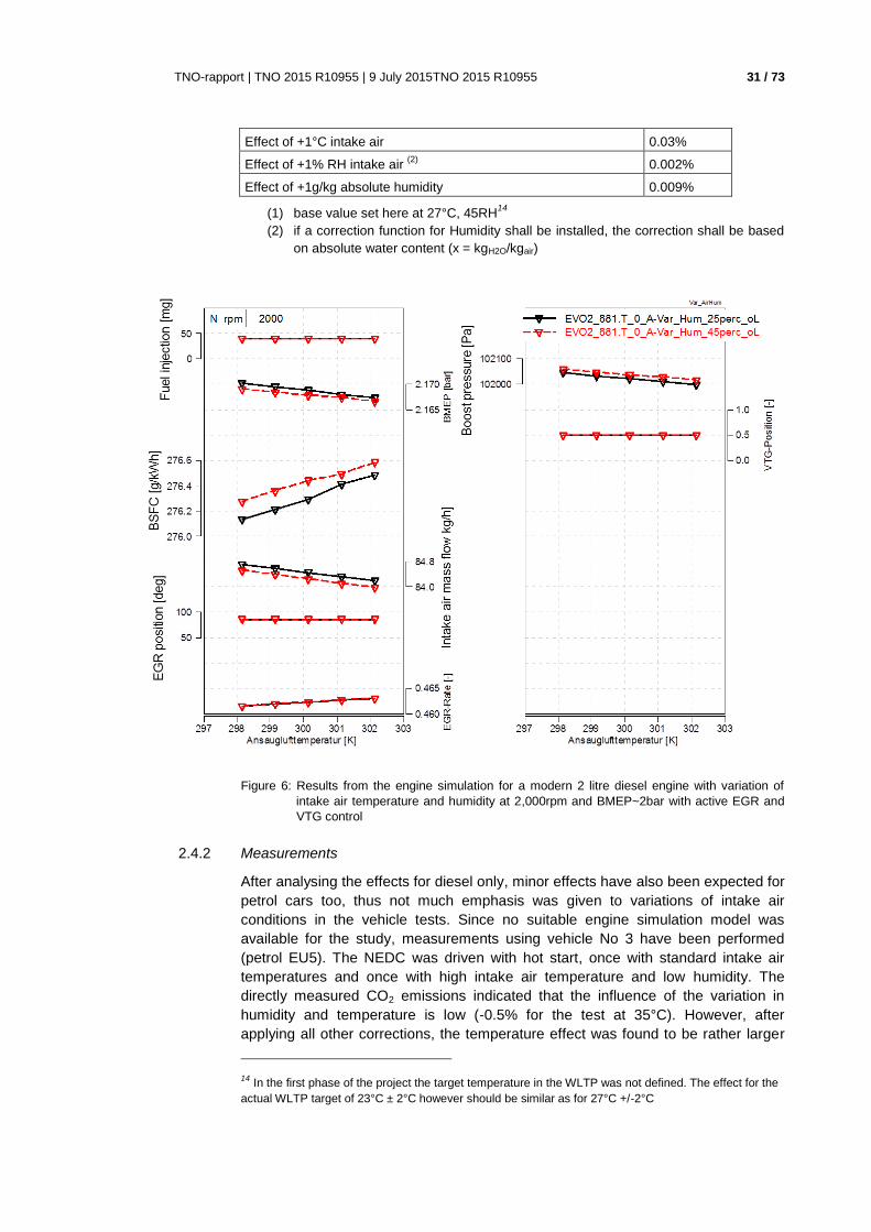
Table 4: Results from the engine simulation for a modern 2 litre diesel engine with variation of
intake air temperature and humidity at 2,000rpm and BMEP~2bar with active EGR and
VTG control
Intake air BSFC Change to base
(1)
[°C] RH X [g/kg] [g/kWh]
25 25% 4.9 276.18 -0.09%
26 25% 5.2 276.21 -0.08%
27 25% 5.5 276.29 -0.05%
28 25% 5.9 276.40 -0.01%
29 25% 6.2 276.47 0.02%
Avg. @25% RH 5.5 276.31 -0.04%
25 45% 8.9 276.27 -0.05%
26 45% 9.4 276.36 -0.02%
27 45% 10.0 276.42 0.00%
28 45% 10.6 276.49 0.03%
29 45% 11.3 276.59 0.06%
Avg. @45% RH 10.0 276.426 0.00%
13 The increase of intake air temperature reduces the air density and thus gives slightly lower air to
fuel ratio which then has a slightly negative impact on the efficiency.
TNO-rapport | TNO 2015 R10955 | 9 July 2015TNO 2015 R10955 31 / 73
Effect of +1°C intake air 0.03%
Effect of +1% RH intake air (2)
0.002%
Effect of +1g/kg absolute humidity 0.009%
(1) base value set here at 27°C, 45RH14
(2) if a correction function for Humidity shall be installed, the correction shall be based
on absolute water content (x = kgH2O/kgair)
Figure 6: Results from the engine simulation for a modern 2 litre diesel engine with variation of
intake air temperature and humidity at 2,000rpm and BMEP~2bar with active EGR and
VTG control
Measurements 2.4.2
After analysing the effects for diesel only, minor effects have also been expected for
petrol cars too, thus not much emphasis was given to variations of intake air
conditions in the vehicle tests. Since no suitable engine simulation model was
available for the study, measurements using vehicle No 3 have been performed
(petrol EU5). The NEDC was driven with hot start, once with standard intake air
temperatures and once with high intake air temperature and low humidity. The
directly measured CO2 emissions indicated that the influence of the variation in
humidity and temperature is low (-0.5% for the test at 35°C). However, after
applying all other corrections, the temperature effect was found to be rather larger
14 In the first phase of the project the target temperature in the WLTP was not defined. The effect for the
actual WLTP target of 23°C ± 2°C however should be similar as for 27°C +/-2°C
TNO-rapport | TNO 2015 R10955 | 9 July 2015TNO 2015 R10955 32 / 73
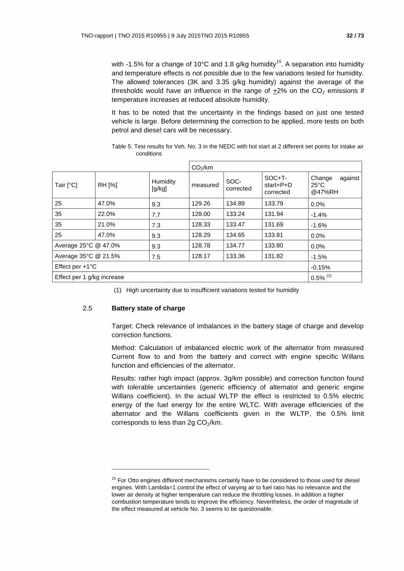
with -1.5% for a change of 10°C and 1.8 g/kg humidity15
. A separation into humidity
and temperature effects is not possible due to the few variations tested for humidity.
The allowed tolerances (3K and 3.35 g/kg humidity) against the average of the
thresholds would have an influence in the range of +2% on the CO2 emissions if
temperature increases at reduced absolute humidity.
It has to be noted that the uncertainty in the findings based on just one tested
vehicle is large. Before determining the correction to be applied, more tests on both
petrol and diesel cars will be necessary.
Table 5: Test results for Veh. No. 3 in the NEDC with hot start at 2 different set points for intake air
conditions
CO2/km
Tair [°C] RH [%] Humidity [g/kg]
measured SOC-corrected
SOC+T-start+P+D corrected
Change against 25°C @47%RH
25 47.0% 9.3 129.26 134.89 133.79 0.0%
35 22.0% 7.7 128.00 133.24 131.94 -1.4%
35 21.0% 7.3 128.33 133.47 131.69 -1.6%
25 47.0% 9.3 128.29 134.65 133.81 0.0%
Average 25°C @ 47.0% 9.3 128.78 134.77 133.80 0.0%
Average 35°C @ 21.5% 7.5 128.17 133.36 131.82 -1.5%
Effect per +1°C -0.15%
Effect per 1 g/kg increase 0.5% (1)
(1) High uncertainty due to insufficient variations tested for humidity
Battery state of charge 2.5
Target: Check relevance of imbalances in the battery stage of charge and develop
correction functions.
Method: Calculation of imbalanced electric work of the alternator from measured
Current flow to and from the battery and correct with engine specific Willans
function and efficiencies of the alternator.
Results: rather high impact (approx. 3g/km possible) and correction function found
with tolerable uncertainties (generic efficiency of alternator and generic engine
Willans coefficient). In the actual WLTP the effect is restricted to 0.5% electric
energy of the fuel energy for the entire WLTC. With average efficiencies of the
alternator and the Willans coefficients given in the WLTP, the 0.5% limit
corresponds to less than 2g CO2/km.
15 For Otto engines different mechanisms certainly have to be considered to those used for diesel
engines. With Lambda=1 control the effect of varying air to fuel ratio has no relevance and the
lower air density at higher temperature can reduce the throttling losses. In addition a higher
combustion temperature tends to improve the efficiency. Nevertheless, the order of magnitude of
the effect measured at vehicle No. 3 seems to be questionable.

TNO-rapport | TNO 2015 R10955 | 9 July 2015TNO 2015 R10955 33 / 73
Magnitude of the influence 2.5.1
The imbalance in battery SOC can have a quite high influence on the test result
although only auxiliaries which are necessary to run the car are consuming energy.
Assuming an average basic electrical load for basic devices of a maximum of
300W, an imbalance of 150 Wh would occur if the energy is taken from the battery
only. With an alternator efficiency of 65% and a Willans coefficient of the engine of
600g CO2/kWh, the effect of such an imbalance would be more than 3 g/km in the
WLTC. If the test is started with an empty battery and the alternator controller
algorithm leads to a battery loading over the cycle, the effect can be much higher.
Similarly, a start with full battery can lead to a discharging at the beginning of the
cycle to provide capacity for eventual following brake energy recuperation, e.g.
Figure 7.
Figure 7: SOC of the battery from a passenger car over a part of the WLTC, once started with an
empty battery and once with full battery
A test started with empty battery led to more than 20% higher CO2 emissions per
km in the WLTC compared to a test started with a full battery (Appendix C), but
such test conditions will hardly occur within the WLTP regulation. When the battery
is charged before the preconditioning test cycle, the SOC at the end of the test is
expected to be for most vehicles already on a normal level which shall not lead to
such large SOC imbalances in the subsequent test.
Option for correction of SOC imbalances 2.5.2
The correction for SOC imbalances can either be based on the vehicle specific
Veline coefficient (kv in g/kWh) or on generic ones. Since the vehicle based Veline
factors are related to the work at the wheel, they would have to be converted into
engine work based values through division by the transmission efficiency. Since the
latter is not known from the chassis dyno test, a generic efficiency would have to be
assumed for different transmission systems. As a consequence of high differences
which can be found in the efficiencies from different transmission systems (manual
and automatic), it seems to be straightforward to use generic engine Willans
factors.
This gives the following correction method:

TNO-rapport | TNO 2015 R10955 | 9 July 2015TNO 2015 R10955 34 / 73
Calculate the imbalance of energy flow from and to the battery:
a) simple option: 𝑊𝑏𝑎𝑡 = ∫ 𝑈(𝑡) ∗ 𝐼(𝑡) ∗ 0.001 𝑑𝑡 in [kWs] with Current flow from
the battery counted with positive sign
The Voltage could also be a generic value of nominal Voltage as suggested in the
WLTP draft (UN ECE 2014). For higher accuracy we may also consider the
charging and discharging losses which lead to the fact that the battery SOC is
reduced if the same electric energy is consumed from the battery as was charged
before. This would lead to the more detailed approach:
b) more detailed option:
𝑊𝑏𝑎𝑡−𝑐ℎ𝑎𝑟𝑔𝑒 = ∫ 𝑈(𝑡) ∗ 𝐼𝑐ℎ𝑎𝑟𝑔𝑒(𝑡) ∗ 0.001 𝑑𝑡 in [kWs] counting only Current to
battery
𝑊𝑏𝑎𝑡−𝑑𝑖𝑠𝑐ℎ𝑎𝑟𝑔𝑒 = ∫ 𝑈(𝑡) ∗ 𝐼𝑑𝑖𝑠𝑐ℎ𝑎𝑟𝑔𝑒(𝑡) ∗ 0.001 𝑑𝑡 in [kWs] counting only Current
from battery
Wbat=Wbat-discharge - (Wbat-charge
×𝑏𝑎𝑡
) in [kWs]
with Bat .............. efficiency of charging and discharging (charge x discharge)
For typical battery systems the can be assumed with
generic values. Draft examples are shown in Table 6.
Table 6: Draft generic combined charge & discharge efficiencies
Efficiency [%]
Pb 87%
Ni-Mh 90%
Li-Ion 97%
Calculate the CO2 correction value from the battery imbalance:
∆CO2SOC [g]=
Wbat
𝑨𝒍𝒕
*ke
with ke ................ Engine Willans coefficient [gCO2/kWs], generic values per
engine technology
Alt............... Generic average efficiency of the alternator including
transmission losses to the engine (in WLTP draft (UN
ECE 2014) an efficiency of 0.67 is suggested. This value
is in line with the results from a simulation with the model
PHEM using alternator efficiency maps)
If a more accurate base shall be provided for setting up the vehicle specific Veline
functions from the SOC corrected WLTP results, the correction shall be done for
each WLTC phase separately. This is more relevant, if the test is started with low
SOC since the vehicle then tends to load the battery from start-up, which mainly
influences the first test phase.
An open question concerning the engine Willans coefficient “ke”, is if and how the
behaviour of smart alternator controllers shall be considered. Basically modern
alternators are loading the battery at engine overrun conditions (brake energy
recuperation). Thus a negative battery energy balance can be attributed mainly to
too low an activity of the alternator in phases with positive engine work. Similarly a

TNO-rapport | TNO 2015 R10955 | 9 July 2015TNO 2015 R10955 35 / 73
positive SOC balance should result mainly from extra alternator activity at phases
with positive engine power16
. If we consider this effect, the correction would have to
be done with the coefficient of a Willans line which is established from test phases
with positive engine power only. The Willans coefficients given in the WLTP (UN
ECE, 2014) seem to originate from positive power values only and thus should be
representative for the SOC imbalance correction.
Temperatures from preconditioning and soak 2.6
Target: Check relevance of the temperature during soak and preconditioning. If
relevant, correct for temperature conditions.
Method: analysis of dependency of friction losses and of fuel consumption as
function of oil temperature and measurement at different temperatures at the
chassis dynamometer
Results: approx. <0.4% impact on CO2 emission result for 2°C deviation against the
target temperature. Generic correction is possible but would need measurement of
oil temperature at test start17
.
Measurements 2.6.1
The influence of variable temperature at test start was found to be a reasonable
influencing factor for the resulting fuel consumption. Nevertheless, the rather
stringent limitation of +/-3°C of cell ambient temperature and +/-3°C for the lube oil
of the vehicle as described in the WLTP draft also limits the effect of deviations
against the target temperature as long as the deviations are within the allowed
boundaries.
The temperature influences the friction losses but also the combustion efficiency.
The combustion efficiency is influenced by the cooler cylinder walls, by different
intake air density (see chapter 2.4) and by the control algorithms applied by the
manufacturer for EGR, VTG and injection timing during heat up. The control
strategies may vary between makes and models, thus a correction function could
either consider only general valid effects, or take combustion efficiency matters into
consideration as a generic average function.
Analysis of existing measurements at engine test stands at TUG for friction losses
as a function of the oil temperature showed that the friction losses at the engine
explain by far not the entire additional fuel consumption at cold starts. Similar tests
on the transmission system and at bear rings to get a complete view on friction
related losses as function of oil temperature were not available. The idea was, to
define generic additional friction losses in the engine and in the transmission as
function of the start temperature to compute the additional work the engine needs to
deliver per °C deviation against the target start temperature. With the engine
Willans coefficients the effect on the fuel consumption could be calculated. This
approach was tested as an option to exclude eventual effects from differences in
engine control at different start temperatures. Figure 8 shows results from an
16 Certainly the amount of brake energy recuperated depends on the alternator power installed.
17 Taking the average cell temperature over e.g. last hour of soaking would add reasonable
uncertainties since temperature at start depends on temperature course over hours with different
weighting of temperature over time.
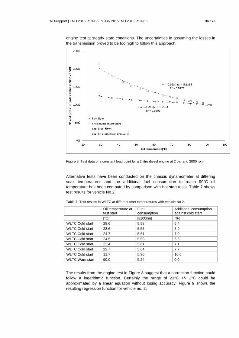
TNO-rapport | TNO 2015 R10955 | 9 July 2015TNO 2015 R10955 36 / 73
engine test at steady state conditions. The uncertainties in assuming the losses in
the transmission proved to be too high to follow this approach.
Figure 8: Test data of a constant load point for a 2 litre diesel engine at 2 bar and 2000 rpm
Alternative tests have been conducted on the chassis dynamometer at differing
soak temperatures and the additional fuel consumption to reach 90°C oil
temperature has been computed by comparison with hot start tests. Table 7 shows
test results for vehicle No.2.
Table 7: Test results in WLTC at different start temperatures with vehicle No 2.
Oil temperature at test start
Fuel consumption
Additional consumption against cold start
[°C] [l/100km] [%]
WLTC Cold start 28.6 5.58 6.4
WLTC Cold start 28.6 5.55 5.9
WLTC Cold start 24.7 5.61 7.0
WLTC Cold start 24.5 5.58 6.5
WLTC Cold start 22.4 5.61 7.1
WLTC Cold start 22.7 5.64 7.7
WLTC Cold start 11.7 5.80 10.6
WLTC Warmstart 90.0 5.24 0.0
The results from the engine test in Figure 8 suggest that a correction function could
follow a logarithmic function. Certainly the range of 23°C +/- 2°C could be
approximated by a linear equation without losing accuracy. Figure 9 shows the
resulting regression function for vehicle no. 2.

TNO-rapport | TNO 2015 R10955 | 9 July 2015TNO 2015 R10955 37 / 73
Figure 9: Additional fuel consumption against hot start conditions as function of oil temperature for
vehicle No. 2 in the WLTC
If just the difference at different start temperatures need to be be calculated, the
logarithmic equation from Figure 9 results in:
Equation 1: ∆𝐹𝐶 = −0.052 ∗ 𝑙𝑛 (𝑡
𝑡𝑟𝑒𝑓)
tref ................ WLTP target temperature (23°C)
Similar tests have been performed with vehicle no. 3 (gasoline EURO 5), which
gave lower effects of the soak temperature.
To base the correction function on a larger database of vehicles, test data from the
ERMES database was used (http://www.ermes-group.eu/web/), which is also the
base data for HBEFA and COPERT emission models. The database includes for
several EURO 5 and EURO 6 cars, hot and cold start NEDC tests (no WLTC yet).
To convert cold start extra emission influences, the percent extra emissions of the
NEDC have been multiplied by 2/3 to compensate for the longer duration of the
WLTC (1800 sec versus 1200 seconds). Then logarithmic regression curves have
been computed to fit the two test values per car (cold start temperature and hot
start). The final correction in the range of 23°C +2°C was then fitted as a linear
function on top of the results from the logarithmic regression line in this temperature
range, as shown in Figure 10.
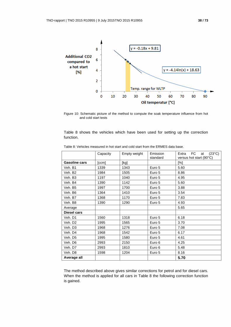
TNO-rapport | TNO 2015 R10955 | 9 July 2015TNO 2015 R10955 38 / 73
Figure 10: Schematic picture of the method to compute the soak temperature influence from hot
and cold start tests
Table 8 shows the vehicles which have been used for setting up the correction
function.
Table 8: Vehicles measured in hot start and cold start from the ERMES data base.
Capacity Empty weight Emission standard
Extra FC at (23°C) versus hot start (90°C)
Gasoline cars [ccm] [kg] [%]
Veh. B1 1339 1343 Euro 5 5.60
Veh. B2 1984 1505 Euro 5 8.86
Veh. B3 1197 1040 Euro 5 4.95
Veh. B4 1390 1142 Euro 5 5.60
Veh. B5 1997 1700 Euro 5 3.88
Veh. B6 1364 1410 Euro 5 3.54
Veh. B7 1368 1170 Euro 5 7.83
Veh. B8 1390 1290 Euro 5 4.93
Average 5.65
Diesel cars
Veh. D1 1560 1318 Euro 5 6.18
Veh. D2 1995 1565 Euro 5 3.70
Veh. D3 1968 1276 Euro 5 7.08
Veh. D4 1968 1542 Euro 5 6.17
Veh. D5 1995 1580 Euro 5 4.61
Veh. D6 2993 2150 Euro 6 4.25
Veh. D7 2993 1810 Euro 6 5.48
Veh. D8 1598 1204 Euro 5 8.16
Average all 5.70
The method described above gives similar corrections for petrol and for diesel cars.
When the method is applied for all cars in Table 8 the following correction function
is gained.

TNO-rapport | TNO 2015 R10955 | 9 July 2015TNO 2015 R10955 39 / 73
∆𝐶𝑂2 = 0,0018 ∗ (𝑡 − 𝑡𝑟𝑒𝑓)
with t .................. Engine oil temperature at test start °C
tref ................ Target temperature in WLTP (23°C)
The CO2 test result corrected for the influence of variable soak temperature is then:
𝐶𝑂2 [𝑔
𝑘𝑚] = 𝐶𝑂2 ∗ (1 + ∆𝐶𝑂2)
Inaccuracy of road load setting 2.7
Target: Check relevance of the inaccuracy of the road load applied at the chassis
dyno. If relevant and possible, elaborate correction method.
Method: measurement of coast down tests on the chassis dyno directly after the
WLTC to establish a method to test the actual values of the road load coefficients.
From differences against the target road load, the difference in the work at the
wheels over the cycle can be computed and corrected with the vehicle Veline
coefficient.
Results: more than 3% impact on the CO2 emission result is possible. It is not clear
yet if the road load measured directly after the WLTC is representative for the road
load during the WLTC. Clarification may need costly measurements with torque
meter rims.
Method 2.7.1
The correction is based on results from coast down tests directly after the WLTC.
The conditions and the evaluation of the coast down shall follow the WLTP
regulation for coast down tests on the test track. The resulting road load values are
then used to compute differences in the work over the cycle against the target road
load values. The effect on CO2 emissions is then calculated from the work
difference with the vehicle Veline coefficient.
Figure 11: Schematic picture of the target coast down and of the coast down result after the WLTC
Using the assumption that the coast down test is representative for the road load in
the WLTC, the correction for the road load would work as follows:

TNO-rapport | TNO 2015 R10955 | 9 July 2015TNO 2015 R10955 40 / 73
Calculate the actual wheel power for the road load coefficients from the chassis
dyno coast down test:
P(j) = (R0 + R1*v(j) +R2*v(j) ² + m*a(j)) * v(j)
Calculate the actual wheel power for the road load coefficients from the target
value:
Pp(j) = (R0w + R1w*v(j) +R2w*v(j) ² + m*a(j)) * v(j)
v(j).......................... velocity driven in the WLTC (average value
between two original speed recordings to fit to the
calculated acceleration as described before
m .......................... vehicle test mass + rotational inertias converted to
equivalent translator mass [kg]
R0, R1 R2 .............. Road load from the coast down tests at the chassis
dyno directly after the WLTC in [N], [N*s/m] and
[N*s²/m²]
R0w, R1w R2w ......... Target road load coefficients in [N], [N*s/m] and
[N*s²/m²]
Then the average power values over the WLTC are computed and consequently
the total work at wheels:
Wwheel = 1.8 x (Pp– P) in [kWs]
If the correction for road load deviations is not combined with the correction for
vehicle speed deviations (chapter 2.2), the calculation of the difference in work can
be simplified, since mass and acceleration are then identical for both road load
settings.
Pp(t)– P(t) = R0w –R0 + (R1w*-R1) *v(t) + (R2w-R2) * v(t) ²
∆𝑾𝐰𝐡𝐞𝐞𝐥 = ∫ (𝑃𝑝(𝑡)
−1800
1
𝑃(𝑡))dt
Then the vehicle based Veline function is applied to correct for the deviation against
the work from the WLTC target velocity:
∆𝑪𝑶𝟐𝒑 [𝒈] = ∆𝑾𝒘𝒉𝒆𝒆𝒍 ∗ 𝒌𝒗
with kv ................ Vehicle Veline coefficient [gCO2/kWs] from WLTP
Test results 2.7.2
In the WLTP (UN ECE, 2014) the preconditioning for measuring the “initial chassis
dynamometer setting load18
”, see WLTP Annex 4 – Appendix 2, seems to be
sufficiently defined, if the criterion given in WLTP Annex 4 paragraph 4.2.4.1.3. has
to also be fulfilled at the chassis dyno test (minimum 20 minutes at defined
velocities). While the preconditioning is defined exactly in the WLTP, the time
between preconditioning and the coast down test for chassis dyno calibration is not
defined. Performing the tests after a shorter warm up or after a longer stand still
before a coast down typically gives higher initial losses from the bearings and
18 There seems to be a small error: in the equation we read “Fdj“ but in the explanation only “Fdi“
appears. IN the actual version from May 2014 the error seems to be corrected.

TNO-rapport | TNO 2015 R10955 | 9 July 2015TNO 2015 R10955 41 / 73
transmission at the roller bench, from the tyres and from the dragged part of the
vehicles transmission and bearings. As a result the “adjustment road load”, which is
the difference between target road load and initial road load, would be rather low to
meet overall the target road load. If the temperature level from roller and the vehicle
is higher in the later WLTC, lower internal losses occur at the roller and from the
vehicle’s tyres, bearings, etc. As a result, for such a scenario the adjusted road load
would be lower in the WLTC than in the initial coast down test. Such insufficient
preconditioning was found to influence the CO2 test results by more than 5%.
Performing the preconditioning according to the WLTP still gave notable deviations
in the road load parameters for some tests (Figure 12 to Figure 14), resulting in
effects on the CO2 emissions of more than 2 g/km (see Appendix C). The deviations
found for the test vehicles did not follow a common trend. For test vehicle No. 3 all
coast down tests that have been performed after NEDC showed the same level
(Figure 13). When applying the road load correction on the NEDC CO2 values, the
correction function consequently shows only small effects (see Appendix C).
Higher differences between target road load and coast down results after the WLTC
tests were found for vehicles No. 2 and 4 (Figure 13 and Figure 14). The
differences between the measured road load values against the target values is
different for R0, R1 and R2 with no uniform trend between the two vehicles tested.
The explanation for the different effects after NEDC and WLTC seems to be, that
after WLTC the state of chassis dyno and vehicle is hotter than after NEDC and
thus the internal losses are a bit lower after WLTC. Since the same effect should
also occur in preconditioning before the initial loss run, the effects found here may
depend on the design of the chassis dynamometer and on details of the procedure
for the initial loss run.
Figure 12: Comparison of the coast down tests after the WLTC tests with the target coast down for
vehicle No. 2
velocity [km/h] 20 60 130
target [N] 0% 0% 0%
chassis test 1 [N] -2.1% -17.4% -10.9%
chassis test 2 [N] -4.5% -17.4% -10.9%
chassis test 3 [N] -5.9% -17.4% -10.9%
chassis test 4 [N] -2.8% -17.4% -10.9%
chassis test 5 [N] -6.2% -17.4% -10.9%
dev.against target
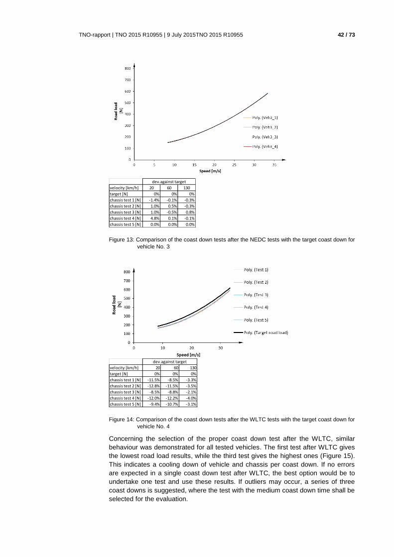
TNO-rapport | TNO 2015 R10955 | 9 July 2015TNO 2015 R10955 42 / 73
Figure 13: Comparison of the coast down tests after the NEDC tests with the target coast down for
vehicle No. 3
Figure 14: Comparison of the coast down tests after the WLTC tests with the target coast down for
vehicle No. 4
Concerning the selection of the proper coast down test after the WLTC, similar
behaviour was demonstrated for all tested vehicles. The first test after WLTC gives
the lowest road load results, while the third test gives the highest ones (Figure 15).
This indicates a cooling down of vehicle and chassis per coast down. If no errors
are expected in a single coast down test after WLTC, the best option would be to
undertake one test and use these results. If outliers may occur, a series of three
coast downs is suggested, where the test with the medium coast down time shall be
selected for the evaluation.
velocity [km/h] 20 60 130
target [N] 0% 0% 0%
chassis test 1 [N] -1.4% -0.1% -0.3%
chassis test 2 [N] 1.0% 0.5% -0.3%
chassis test 3 [N] 1.0% -0.5% 0.8%
chassis test 4 [N] 4.8% 0.1% -0.1%
chassis test 5 [N] 0.0% 0.0% 0.0%
dev.against target
velocity [km/h] 20 60 130
target [N] 0% 0% 0%
chassis test 1 [N] -11.5% -8.5% -3.3%
chassis test 2 [N] -12.8% -11.5% -3.5%
chassis test 3 [N] -8.5% -8.8% -2.1%
chassis test 4 [N] -12.0% -12.2% -4.0%
chassis test 5 [N] -9.4% -10.7% -3.1%
dev.against target

TNO-rapport | TNO 2015 R10955 | 9 July 2015TNO 2015 R10955 43 / 73
Figure 15: Results of 3 consecutive coast down tests after the WLTC for vehicle No. 2 in
comparison to the target road load
An alternative to the road load correction would be a precise definition of the
calibration procedure for the road load settings at the chassis dynamometer. This is
assumed to give similar effects for the reproducibility but requires less effort in
testing and in test evaluation.
A draft for the amendments necessary in the WLTP to better define the procedure
for adjusting the road load to the chassis dynamometer is given in Annex G.2.
Electrified vehicles 2.8
The main effect to consider is how the battery charging/discharging losses have to
be considered in the energy balance.
A similar approach as for SOC imbalances in chapter 2.5 is possible. A more
detailed elaboration could be started after discussion if this option fits into the actual
discussion on HEV.
Gear shifts 2.9
Target: Check relevance of deviations against target gear shift points and develop
correction function if possible.
Method: simulation with Passenger car and Heavy duty Emission Model (PHEM) to
obtain influence of gear shift variations.
Results:
The gear shift points influence the vehicle’s fuel consumption (FC) to a large extent.
For the FC investigation of different gear shift points in WLTC, various simulations
with one petrol engine and one diesel engine were performed to test the sensitivity
of the fuel consumption against small deviations in gear shift timing.
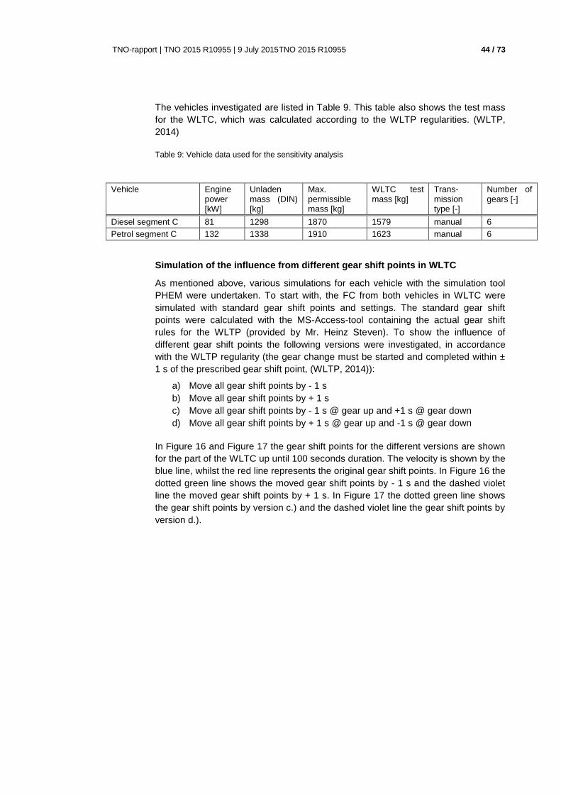
TNO-rapport | TNO 2015 R10955 | 9 July 2015TNO 2015 R10955 44 / 73
The vehicles investigated are listed in Table 9. This table also shows the test mass
for the WLTC, which was calculated according to the WLTP regularities. (WLTP,
2014)
Table 9: Vehicle data used for the sensitivity analysis
Vehicle Engine power [kW]
Unladen mass (DIN) [kg]
Max. permissible mass [kg]
WLTC test mass [kg]
Trans-mission type [-]
Number of gears [-]
Diesel segment C 81 1298 1870 1579 manual 6
Petrol segment C 132 1338 1910 1623 manual 6
Simulation of the influence from different gear shift points in WLTC
As mentioned above, various simulations for each vehicle with the simulation tool
PHEM were undertaken. To start with, the FC from both vehicles in WLTC were
simulated with standard gear shift points and settings. The standard gear shift
points were calculated with the MS-Access-tool containing the actual gear shift
rules for the WLTP (provided by Mr. Heinz Steven). To show the influence of
different gear shift points the following versions were investigated, in accordance
with the WLTP regularity (the gear change must be started and completed within ±
1 s of the prescribed gear shift point, (WLTP, 2014)):
a) Move all gear shift points by - 1 s
b) Move all gear shift points by + 1 s
c) Move all gear shift points by - 1 s @ gear up and +1 s @ gear down
d) Move all gear shift points by + 1 s @ gear up and -1 s @ gear down
In Figure 16 and Figure 17 the gear shift points for the different versions are shown
for the part of the WLTC up until 100 seconds duration. The velocity is shown by the
blue line, whilst the red line represents the original gear shift points. In Figure 16 the
dotted green line shows the moved gear shift points by - 1 s and the dashed violet
line the moved gear shift points by + 1 s. In Figure 17 the dotted green line shows
the gear shift points by version c.) and the dashed violet line the gear shift points by
version d.).

TNO-rapport | TNO 2015 R10955 | 9 July 2015TNO 2015 R10955 45 / 73
Figure 16: Visualization of different gear shift points, version a.) and version b.)
Figure 17: Visualization of different gear shift points, version c.) and version d.)
The FC calculated from the different cases are listed in Table 10. Cases No. 1 and
No. 6 give the FC for the petrol and diesel engine with standard gear shift points
and settings. The FC deviations from the other cases (expressed as a percentage)
are based on the corresponding basis vehicle.
As expected, version c.) gives the lowest FC for both engines with 1.2 % FC
reduction for the diesel vehicle and 1.1 % reduction for the petrol vehicle. With
version d.), the FC increases by 1.6 % for the diesel engine and 1.4 % for the petrol
engine. The FC deviations from the other versions are between the best and worst
case values.

TNO-rapport | TNO 2015 R10955 | 9 July 2015TNO 2015 R10955 46 / 73
Table 10: FC regarding different gear shift points
No. Vehicle Cycle Gear shift points FC [g/km] Delta [%]
1 Diesel segment C
WLTC Not modified 39.07 0.0 %
2 Move by + 1 s 39.57 1.3 %
3 Move by - 1 s 38.69 - 1.0 %
4 Move by - 1 s @ gear up and + 1 s @ gear down
38.58 - 1.2 %
5 Move by + 1 s @ gear up and - 1 s @ gear down
39.68 1.6 %
6 Petrol segment C
Not modified 54.06 0.0 %
7 Move by + 1 s 54.68 1.1 %
8 Move by - 1 s 53.57 - 0.9 %
9 Move by - 1 s @ gear up and + 1 s @ gear down
53.44 - 1.1 %
10 Move by + 1 s @ gear up and - 1 s @ gear down
54.81 1.4 %
Possible correction functions
Corrections could be applied only if the change in gear shifts against the target is
known. Deviations could be computed from a measured engine speed signal. A
correction function could then be based on generic functions for change in FC over
change in rpm. A simple, but less accurate, option could be based on integration of
deviations in gear shift time against the target in total seconds. A generic function
for change in FC over the integrated time deviation for the gear shift manoeuvres
could then be established. Further details need to be elaborated if it is clear that an
engine speed signal would be available from type approval tests.
To be completed if reasonable idea comes up.
Accuracy of relevant sensor signals for correction functions 2.10
The correction methods demand accurate input data to improve the accuracy of the
CO2 test result. The accuracy of the input signal needs to be clearly higher than the
range in which the signal shall be corrected. E.g. a correction for +2°C oil
temperature at the test start, needs an accuracy of the temperature signal much
better than 2°C to achieve an overall improvement.
Table 11 summarizes the actual definitions in the WLTP (UN ECE, 2014) and the
requirements for applying the correction functions. Certainly the requirements can
be discussed to find a compromise between effort and accuracy, but the following
signals seem to need higher accuracy than stated in the WLTP:
Vehicle speed: relevant for correction of deviations against target speed; at
130 km/h, 1.3 km/h inaccuracy is allowed according to WLTC. It seems not
to be reasonable to correct +2 km/h deviation with such sensor inaccuracy.
Oil temperature of the vehicle: relevant for correction of start temperature.
No definition of the position of such a sensor and of the sensors accuracy
was found in WLTP.
Test cell temperature and humidity: if a correction of intake air conditions
shall be applied, much higher accuracy than demanded in the WLTP would
be necessary.

TNO-rapport | TNO 2015 R10955 | 9 July 2015TNO 2015 R10955 47 / 73
Table 11: Accuracies defined in WLTP for the input data relevant for the correction functions
elaborated before
Signal Accuracy demanded in
WLTP
Accuracy necessary for proper
correction function
Vehicle speed and
chassis dyno roller
speed
± 0.5 km/h or ± 1 per cent,
whichever is greater
If a deviation against target velocity within
a tolerance of +2km/h shall be corrected,
the accuracy of the speed signal needs to
be at least less than 0.5 km/h also at
higher velocities if deviations of <2km/h
shall be corrected.
Time accuracy: min. ± 10 ms; time resolution:
min. ± 0.01 s
Sufficient
Wheel torque (per
torque meter):
± 3 Nm or ± 0.5 per cent of the
maximum measured torque,
whichever is greater
Signal not used for corrections here.
Torquemeter wheel rims allow accuracies
of up to 0.25 per cent (ACEA, 2014). The
0.5% seems to be reasonable.
Chassis dynamometer
force
± 10 N or ± 0.1 per cent of full
scale, whichever is greater
Signal not used, accuracy seems to be
sufficient.
Test cell ambient air
temperature
accuracy of ± 1.5 K
Measured at vehicle cooling
fan outlet
Not sufficient for correction of intake air
temperature in a tolerance of ± 5 K. In
(MAC, 2014) temperature sensors with
accuracy of ≤ ±0.3K+0.005*t are
requested, that gives ± 0.5 K.
DIN IEC 751 also defines for class B:
0.30+0.005 * t. This could be a
reasonable demand also for the WLTP.
Position of sensor seems to be suitable.
Test cell absolute
humidity (Ha)
accuracy of ±1 gH2O/kgair
Measured at vehicle cooling
fan outlet.
A total tolerance of 6.7 gH2O/kgair is
defined in WLTP, thus more accurate
sensors seem to be advantageous. In the
actual draft for the MAC test procedure
an accuracy of < 0.2 g/kg at +20..30 °C
(i.e. ±1% for a range between 35% to
55% RH) is demanded (MAC, 2014).
Position of sensor seems to be suitable.
Current transducer accuracy of 0.5 per cent of the
measured value (in A) or
0.1 per cent of full scale
deflection, whichever is
smaller.
Seems to be sufficient, (MAC, 2014)
refers to the WLTP in this case.
Oil temperature No definition of accuracy
found in WLTP yet
If the soak temperature shall be corrected
in the range of +2°C, an accuracy of the
sensor according to DIN IEC 751 class A
(0.15+0,002 * t) seems to be necessary.
In addition a representative location for
temperature measurement would be
necessary.

TNO-rapport | TNO 2015 R10955 | 9 July 2015TNO 2015 R10955 48 / 73
3 WLTP coast-down test procedure
The coast down testing for road load determination consists of four major parts:
1. Vehicle and tyre preparation
2. Conditioning
3. Coast down testing
4. Data analysis
The WLTP legislative text is based on the NEDC text. The approach is similar,
although some major conceptual changes are introduced. An important change is a
switch from coast-down time to coast-down power in the evaluation. The approach
is still a mixture of time and power (i.e., the reciprocal of time), however, the central
theme is that the difference in force in the “a” and “b” run, as the result from wind
and test-track slope, are properly added to yield a limited net force.
Many other changes in the text are related to stricter conditions and a more precise
formulation of the procedure. In particular, tyres to be used are specified in terms of
tyre label, wear, and pressure. Also the weight of the vehicle is typically higher,
matching better the typical production vehicle weights.
Corrections included in the WLTP 3.1
In the WLTP a number of corrections are already included in Annex 4 for arriving at
a standardized road load:
Wind correction (GTR Annex 4 section 4.5.3) 3.1.1
Based on the ‘a’ and ‘b’ test together, there is a small remaining force resulting from
a larger increase of the air drag into the wind the wind, than a reduction of the air
drag with the wind from behind. The correction is based on the vector addition of
both tests, combined with the assumption that the air drag is of the generic form:
Force [N] = F2 * v2
The combination of the quadratic form, and the factor “F2” yields a correction for
wind of the same form:
Fwind = F2 * vwind2
To be subtracted from the observed force.
Air density (GTR Annex 4 section 4.5.1) 3.1.2
The correction for the air density, also relies on assigning air drag solely to F2 and
the use of the ideal gas law:
Density ~ Pressure/Temperature
Only negligible errors are made by using the ideal gas law. No systematic study into
the assignment of air drag to F2 has been found. Furthermore, the onset of
turbulence and the resulting wall flow thickness is considered a major influence. For
example, it is taken into account in the design of edge curvatures of the A-stile.

TNO-rapport | TNO 2015 R10955 | 9 July 2015TNO 2015 R10955 49 / 73
The onset of turbulence is affected by the temperature through viscosity. These
effects do not find their way into the correction procedure as it is considered too
complex. No impact of air density on F1 is assumed in the WLTP, as the nature of
F1 is not fully known.
Tyre viscosity (GTR Annex 4 section 4.5.2) 3.1.3
The temperature of the tyre, reducing the hysteresis loop and viscous losses in the
tyre, is included in a WLTP correction. In this correction the ambient temperature is
used. However, tyres heat up, and this may depend on solar radiation, road surface
temperature, blue sky, precipitation, etc.. None of these underlying effects are taken
into account in the correction. However, in the test program the magnitude of the
correction is found to be correct. Hence, it can be accepted as an appropriate
correction with temperature, however, not based on a sound physical model
incorporating all major effects. Furthermore, as in air drag, also here the separation
between rolling resistance and air drag is an assumption, globally correct, but the
F1 term in the road load seems to carry both air-drag and rolling resistance effects.
In the legislative text F0 and F1 are assigned to rolling resistance, F2 to air drag.
Test mass correction (GTR Annex 4 section 4.5.4) 3.1.4
The correction for a different test mass is based on the assumption that rolling
resistance acts like friction: the forward force is proportional to the vertical force, or
weight. In first order, this is a correct assumption, based on different
measurements, and on the different underlying physical phenomena with constitute
together the total rolling resistance. Hence the correction for test mass variations is
proportional with the rolling resistance:
F0 = F0test * (TMreference/TMtest)
The meaning of the F1 term 3.1.5
The WLTP relies of the road load coefficients F0, F1, and F2 to apply the
corrections. The air-drag is associated with F2, and air drag correction, like the air
density, are applied to F2. The terms F0 and F1 are associated with rolling
resistance. This is an ‘a priori’ assumption. In particular F1 has a dubious status,
which may combine rolling resistance, transmission losses, and air drag effects. It is
quite common that F1 is negative. For example the EPA certification data of 2013
has 10% of the road load values below zero, i.e., a negative effect.
It may very well be that in the transition to turbulent flow as the velocity increases,
the air drag initially increases before the eventual drop in air drag associated with
developed turbulent flow. This is related to boundary layer thickness, and flow
separation at the tail of the vehicle. In that case F1 may indicate something of this
transition.
The velocity dependence of rolling resistance is also changing. This affects the
meaning of F1 and F2, which can incorporate some rolling resistance. Traditionally,
a linear increase with velocity existed, however with modern radial tyres the rolling
resistance remains nearly constant up to high velocities, with an increase above
100-120 km/h. This would suggest a velocity dependence that is more properly part
of F2 than F1.
Since F0, F1, and F2 are the result of fitting procedure coast-down time-interval
data, the effects are not separated. The assignment of F2 to air-drag can lead to a

TNO-rapport | TNO 2015 R10955 | 9 July 2015TNO 2015 R10955 50 / 73
minor overestimation of the correction in the order of 10%. Likewise, equating F0
and, especially, F1 to rolling resistance, some corrections of the rolling resistance,
such as the mass correction, may lead to a minor deviation.
Coast-down test 3.1.6
Coast down testing is performed to determine the resistance of the vehicle to
motion. It requires a certain amount of power to keep a vehicle in motion at a
constant velocity. In the absence of acceleration or deceleration, this is the friction
force of the vehicle: internally, the contact of the tyres, and the air drag constitute
this force. Especially at higher velocities, the engine is used mainly to overcome this
resistance. In the laboratory, on the chassis dynamometer test, this resistance,
determined in the coast-down test, is reproduced to ensure the same engine load
as on the road is associated with the laboratory test.
The force balance in Newtons [N] of a vehicle is given by:
(M + mr) * a = Fdriveline + Frolling + Fair-drag ~ F0 + F1 * v + F2 * * v2
Where:
M: the weight of the vehicle [kg]
mr: the rotational inertia of the vehicle (Imoment/R2) [kg]
a: the acceleration (a = dv/dt) [m/s2]
Fx : the respective forces [N]
v: the velocity [km/h]
F0, F1, F2: the road-load coefficients [N, N/(km/h), N/(km/h)2]
Typically, F0 is associated with driveline and rolling resistance and F2 with air-drag.
The rolling resistance is dominant over the driveline, during the coast-down test
when the clutch is disengaged. The coefficient F1 can be positive or negative,
depending on the details at intermediate velocities. This term in the polynomial
affects mainly the total resistance between 30 and 80 km/h. However, this
coefficient, and the association is an approximation. Rolling resistance is known to
increase at high velocities. Furthermore, the generic formula, such as the Streibeck
formula, shows also an increase in resistance torque in driveline bearings with an
increase in rotational velocity, from a baseline value at low speeds.
The air-drag is often approximated by:
Fair-drag ~ ½ * Cw * rhoair * v2 * Afrontal
where rhoair is the air density [kg/m3]; v
2 the square of the velocity [m/s]; Afrontal[m
2]
the frontal area of the vehicle; and Cw the aerodynamic drag coefficient associated
with the shape of the vehicle. This is typically in the range of Cw ~ 0.25-0.5 for
passenger cars (higher for heavy-duty vehicles and powered two-wheelers). Note,
this formula is based on a turbulent flow around the vehicle, and is better suited for
high velocities than low velocities.
Tyres have rolling resistance coefficients (RRC [-]), which, combined with the
vertical force on the wheel, yield the resistance force. Tyre labels are based on
these coefficients, and therefore seem to suggest that the rolling resistance is
proportional to the weight of the vehicle. This is a good first order approximation:
Frolling ~ RRC * M * g

TNO-rapport | TNO 2015 R10955 | 9 July 2015TNO 2015 R10955 51 / 73
where M is the weight of the vehicle, and g = 9.81 m/s2 the gravitational constant
converting weight to force.
Since the type-approval test consists of two parts: the coast-down test and the
chassis dynamometer, there are a number of issues concerning the use of the
coast-down results on the chassis dynamometer. Traditionally, there has been quite
a lot of flexibility in the NEDC test procedure for the limitations of the chassis
dynamometer. However, this does not take away from the fact that fundamentally
the vehicle should have the same coast-down test results on the chassis
dynamometer as on the road (see Figure 18). This involves the following three
aspects:
1. The same vehicle, as much as possible. This includes the same weight and
wheels.
2. Correct inertia settings, or weight of the vehicle (with the inclusion of the
rotating inertia of a stationary axle on the chassis dynamometer)
3. The same power, or rolling resistance. This can be a limited number of
settings, for example, power at 80 km/hr, or the three values F0, F1, and
F2,. However, preferably, the power settings at all the different velocities
reported in the coast-down test are determined and compared with the
coast-down test..
The rotating inertia is a complicating factor in the test. If all axles were rotating there
would be no problem. It is the stationary axle which creates a mismatch between
the two coast-down tests. A fixed 1.5% (e.g. 21 kg for a 1,400 kg vehicle) of the
vehicle weight is assumed, which is an appropriate average value, but which may
deviate substantially in some cases. Moreover, the use of different wheels and
tyres, complicates the relation between the coast-down test and chassis
dynamometer test.
Figure 18”: The best guarantee that the road-load settings are appropriate, is if the coast-down
test is repeated on the chassis dynamometer, with the same total inertia. The coast-
down test on the chassis dynamometer should follow the WLTP test immediately.
There are several alternative ways of matching the coast-down test and the chassis
dynamometer settings. Also, traditionally values are reported which exclude the tyre
rolling resistance. These different approaches allow for flexibilities in the settings.
Ideally, the coast-down test on the chassis dynamometer test will tell if all these
settings add up to the appropriate net result.
Chassis-dynamometer coast down
On-road coast down
velocity
matching

TNO-rapport | TNO 2015 R10955 | 9 July 2015TNO 2015 R10955 52 / 73
The same roll-out times on the road and on the chassis dynamometer should be
achieved only in the case of the same vehicle inertia. Roll-out times are inversely
proportional with the inertia. Hence, in the case of a different inertia for both tests, it
should be corrected for:
Tchassis-dynamometer/Tcoast-down = (M+mr)coast-down/(M+mr)chassis-dynamometer
This is the correction applied to the coast-down. The carry-over to the chassis
dynamometer is not fully covered.
Vehicle preparation 3.2
The vehicle must be in proper running order for a coast-down test. This includes
removing parasitic braking, setting wheel alignment, and setting the tyre pressure.
These factors are very important for the eventual road-load values. Other
preparation includes the setting of inlet vanes, removal of optional fixtures such as
antennae, and the setting of fixtures. Also cleaning the car may have a small effect
of the air flow friction.
The wheel alignment was found to affect the rolling resistance substantially. For the
tested vehicle, changing the toe-in from 0.2o to 0.0
o reduced the rolling resistance
by 6%. It is difficult to generalize this result, as limited information is available of the
physical nature of the effect. The findings from the validation program may not
apply to other tyres and suspension.. Instead it would be appropriate to test the
vehicle with the maximal value away from upright and parallel wheels, in the range
prescribed by the manufacturer.
WLTP text proposal:
The alignment of the wheels: toe-in and camber, should be set
to the maximal deviation from the parallel positions in the
range of angles defined by the manufacturer. If a
manufacturer specifies a set value, with a tolerance, this
value may be used.
Discussion in WLTP IWG resulted in an adoption of the
following text in WLTP gtr Phase 1b:
“4.2.1.7.3 Wheel alignment
Toe and camber shall be set to the maximum deviation from the
longitudinal axis of the vehicle in the range defined by the
manufacturer. If a manufacturer prescribes values for toe and
camber for the vehicle, these values shall be used. At the
request of the manufacturer, values with higher deviations
from the longitudinal axis of the vehicle than the prescribed
values may be used. The prescribed values shall be the
reference for all maintenance during the lifetime of the car.
Other adjustable wheel alignment parameters (such as caster)
shall be set to the values recommended by the manufacturer.
In the absence of recommended values, they shall be set to
the mean value of the range defined by the manufacturer.
Such adjustable parameters and set values shall be recorded.”

TNO-rapport | TNO 2015 R10955 | 9 July 2015TNO 2015 R10955 53 / 73
Vehicle conditioning 3.3
The vehicle is prepared for coast down by driving at a high velocity for at least 20
minutes. The result is a warming up of the components of the vehicle. The
lubricants will be warmer, but also the tyres will be warmer and the tyre pressure
increases. Furthermore, the engine block will be warm and will radiates heat
throughout the test. In practice , it is very difficult to control these heat transfers
throughout the test. Testing on a colder test track surface, or testing in sunnier
conditions, will all affect the loss of heat and thereby the tyre temperature. The only
way to standardize the test is to measure the tyre pressure sufficiently often
throughout the test, and correct for the tyre pressure.
WLTP text proposal:
The tyre pressure during the test is increased due to the
preconditioning. This pressure increase must be appropriate
for the preconditioning driving. During the test moderate
driving, maximal velocity appropriate for the coast-down
velocities, limited braking, and limited exposure of the
tyres to heat must be maintained.
The lubricant oil of the driveline in motion during coast down can also be affected by
specific heat transfer conditions. However, this effect is considered secondary to
the effect of the actual tyre pressure during the test.
Coast-down test 3.4
During the test, fuel is consumed which decreases the weight of the vehicle. If the
test is divided in four parts, and ten repetitions of each are needed, the fuel
consumption of such a test may already be as high as 5-10 litres for a passenger
car, which weight differences on a 1,200 kg vehicle are not fully neglible. However,
no correction of the test result or adaptation of the WLTP procedure is proposed, as
the impact is much smaller than the observed test to test variations in coast-down
times.
Two major aspects affect the outcome of the individual coast-down tests: Firstly, the
local wind conditions, both in the point of time and the position along the track,
which can be 3 kilometres long. Secondly, the tyre pressure, which will fluctuate
with the internal temperature. The tyre pressure can be 10%, or more, higher during
the test than prior to the conditioning. The amount of heat dissipated in a tyre, at
high velocities, can be close to 1,000 Watt. At lower velocities, the amount of heat is
less; proportional with the velocity. The internal heat is not simply lost. Hence high
temperature and the resulting high tyre pressures will affect the outcome of the test.
Considering most energy lost though rolling resistance is heat, the heat production
can be estimated. The generated heat per tyre is approximately:
Heat [W] = 2.725 * RRC * Mtyre[kg] * v[km/h] ~ 4-8 * v[km/h]
where Mtyre is the weight on the tyre.
Most kinetic energy dissipated in the tyre rolling resistance is converted to heat,
with only a small amount dissipated as noise, or transferred as vibration to the
vehicle.

TNO-rapport | TNO 2015 R10955 | 9 July 2015TNO 2015 R10955 54 / 73
Tyres are heated through three main processes:
First, the viscoelastic deformation of the tyre, converting work into heat.
Most of the rolling resistance is converted in this manner;
Second, the contact of the tyre profile with the road surface, causing local
deformation of the tyre; and
Third, the friction of the tyre on the road. A large amount of energy can be
converted to heat in this manner, which, however, requires slip of the tyre
over the surface. This slip is common for bends, but not so much so in
forward motion, i.e., rolling of the tyre.
Furthermore, the tyre can be heated or cooled by the surroundings. This heating or
cooling results mainly from road surface contact, air convection, solar radiation,
radiation from the engine block and heat transfer from brakes.
Figure 19: The heat generation and heat transfer of a tyre is a complex process with many
variables which cannot be determined easily.
Rubber has a low heat conductance, such that 1,000 Watt heat transfer across the
rubber may yield a temperature difference of 60-80 degrees Celsius. The
associated tyre pressure increase is 20%. This is confirmed by the validation
measurements. The outer surface of the tyre may be lukewarm, but this is not a
proper indication of the temperature inside the tyre, and the associated tyre
pressure which varies with internal temperature.
A vehicle driving up and down a straight test track and turning at each end, will
have a different intermediate velocity profile between coast-down test than a vehicle
on an oval test track, where in the bends not only can high velocities be achieved,
but also the friction from the lateral force can be substantial. Furthermore, the low
velocity coast-down tests may or may not have in-between accelerations to high
velocity. As a result it is almost impossible to prescribe the driving which leads to
the tyre pressure. Instead the tyre pressures must be monitored at regular intervals.

TNO-rapport | TNO 2015 R10955 | 9 July 2015TNO 2015 R10955 55 / 73
Figure 20: Typical test execution may take more than two hours to reach the prescribed accuracy
of 3%. The warm-up or pre-conditioning is less relevant for the state of the tyre in the
second half of the test.
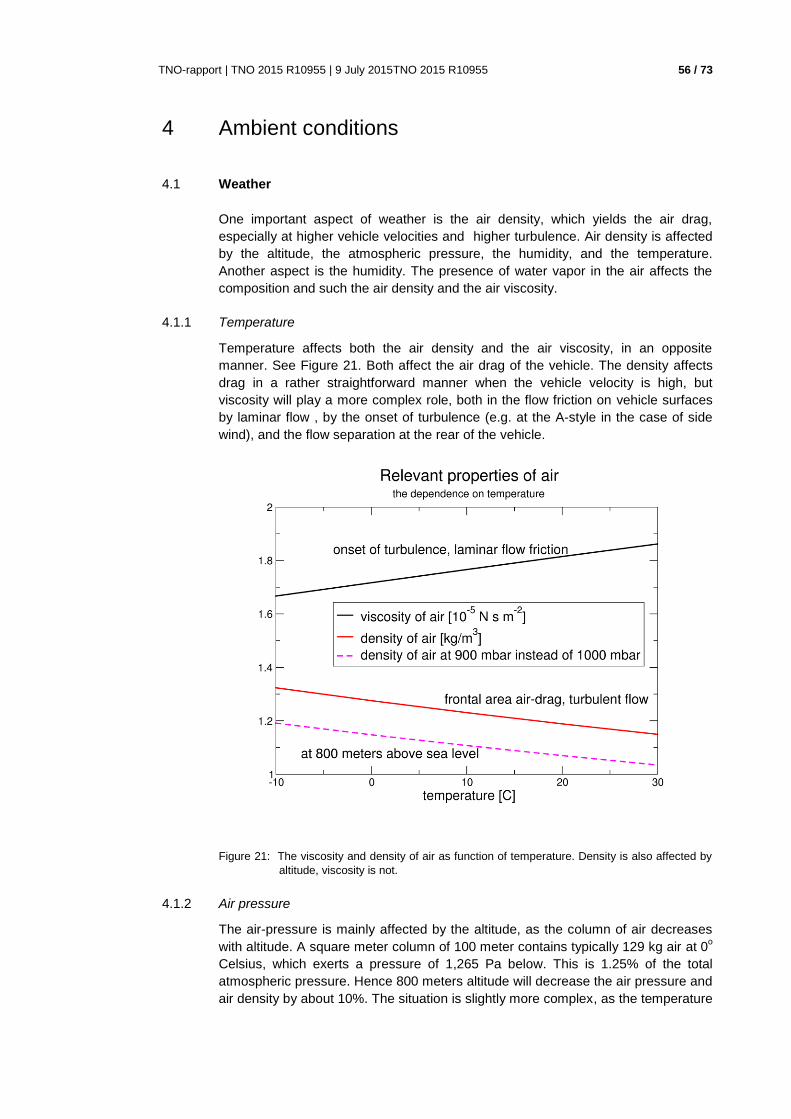
TNO-rapport | TNO 2015 R10955 | 9 July 2015TNO 2015 R10955 56 / 73
4 Ambient conditions
Weather 4.1
One important aspect of weather is the air density, which yields the air drag,
especially at higher vehicle velocities and higher turbulence. Air density is affected
by the altitude, the atmospheric pressure, the humidity, and the temperature.
Another aspect is the humidity. The presence of water vapor in the air affects the
composition and such the air density and the air viscosity.
Temperature 4.1.1
Temperature affects both the air density and the air viscosity, in an opposite
manner. See Figure 21. Both affect the air drag of the vehicle. The density affects
drag in a rather straightforward manner when the vehicle velocity is high, but
viscosity will play a more complex role, both in the flow friction on vehicle surfaces
by laminar flow , by the onset of turbulence (e.g. at the A-style in the case of side
wind), and the flow separation at the rear of the vehicle.
Figure 21: The viscosity and density of air as function of temperature. Density is also affected by
altitude, viscosity is not.
Air pressure 4.1.2
The air-pressure is mainly affected by the altitude, as the column of air decreases
with altitude. A square meter column of 100 meter contains typically 129 kg air at 0o
Celsius, which exerts a pressure of 1,265 Pa below. This is 1.25% of the total
atmospheric pressure. Hence 800 meters altitude will decrease the air pressure and
air density by about 10%. The situation is slightly more complex, as the temperature

TNO-rapport | TNO 2015 R10955 | 9 July 2015TNO 2015 R10955 57 / 73
also decreases due to adiabatic relation between the air in the column, which
results in a lower temperature at higher altitudes. On the other hand, as the density
decreases with the altitude, so the column weight also decreases.
The air pressure itself may fluctuate with the weather, with times of stable high
pressure alternating with times of low pressure fronts. The normalized sea-level air
pressure is 101.325 kPa. The maximal range of air pressure variation, at the
weather station at sea level close to the main test track is between -14% and +7%,
however typical fluctuations in the air pressure are -2% and 2% around the
standard air pressure.
Figure 22: The average over 2000-2010 of the air pressure at the location of the Katwijk test track.
The variations are limited and evenly distributed.
The normal air pressure used in the WLTP text is 100 kPa. At sea level it is at the
edge of the distribution in Figure 22, however, at an altitude of about 110 m, the
average air pressure is around 100 kPa. The latter value is used as reference in the
WLTP text. This value is appropriate for European conditions, suggesting testing at
a higher altitude than sea level.
Air composition 4.1.3
At high temperatures, the water vapour content of air may be substantial: 4.1% at
30o Celsius, and 7.3% at 40
o Celsius. This will lower the air density slightly, as
water vapour has 37.7% lower density than air. Hence, the maximal net effect of
high humidity is 1.5% at 30o, and 2.6% at 40
o Celsius. This is for 100% relative
humidity. In saturated airmist or fog may form, which increases the density again.
The latter is unfavorable for the air drag. The variation of the viscosity with the water
vapor content is expected to be maximal in the order of 2%, based on the mixing
rule of Wilke, where the viscosity of water vapor is lower than that of air, and an
increase in relative humidity decreases the viscosity. Since the viscosity, i.e., the
wall friction for laminar flow, is only a minor part in the total air drag, the impact of
humidity on viscosity can be discounted.

TNO-rapport | TNO 2015 R10955 | 9 July 2015TNO 2015 R10955 58 / 73
For the relationship between the relative humidity and the absolute water vapour
content in air, the approximation on Antoine is often used.
Pvapour[bar] = 157000*10-1730.63/(233.46+T[C])
See Figure 23.
Figure 23: The absolute molar water content of saturated air for different temperatures.
The water vapour content can be used to adjust the air density with relative
humidity and temperature:
Pvapour/Pambient
The fraction of water vapour is multiplied with the ratio of densities to arrive at the
density ratios:
1 – 0.37* Pvapour/Pambient
Using dry air as a reference will only affect the air density at the reference
temperature by a small amount. At 300 K the water vapour content is still limited
resulting in 0.2%-0.3% density variations with varying humidity.

TNO-rapport | TNO 2015 R10955 | 9 July 2015TNO 2015 R10955 59 / 73
WLTP text proposal:
The air-drag must be compensated for the deviation of the air
density. The air density is proportional with pressure p and
inversely proportional with temperature T, such that the
observed air drag is compensated with factor (100/p)*(T/300).
Furthermore, the air drag must be compensated for the
presence of water vapour through a factor
1+0.37*Pvapour/Pambient, assuming the standard condition is
dry air.
“4.5. Correction to reference conditions
4.5.1. Air resistance correction factor
The correction factor for air resistance, K2, shall be
determined as follows:
K2 = T
293×
100
P× (1 + 0.37 ×
𝑃𝑣𝑎𝑝𝑜𝑟
𝑃)
where:
T is the mean atmospheric temperature, K;
P is the mean atmospheric pressure, kPa;
Pvapour can be either measured directly or determined from the
relative humidity (RH) measurement by the formula
Pvapour = RH *15700000*10-1730.63/(-39.67+T[K]), kPa;”
Note: outcome is exactly 101.39 kPa at 100 0C and RH=1.
Wind 4.2
Wind is one of the most dominant uncontrollable aspects which affects the coast-
down results. For European on-road conditions the effect for a single direction is
about 10% on the coast-down times and road loads. For a round trip: both
directions, the net effect is much smaller. It is estimated to be in the order of a few
percent. This depends very much on the vehicle velocity and shape.
Wind speed 4.2.1
For meteorological data, the wind speed is measured at 10 metres, or 30 feet,
above the ground level. The wind velocity at 10 metres is higher, and more constant
than at 0.5-1.5 metres height, which is relevant for the air drag of vehicles.
Measurements at 0.7 metres height show a larger variation in wind speeds and
wind direction compared with the meteorological station Katwijk, from the Dutch
Meteorological Service (KNMI), nearby at 100 metres distance and at 10 metres
high.
The relation between wind speeds at different altitudes is not fixed, but dependent
on the meteorological conditions. Stable conditions, with a small temperature
TNO-rapport | TNO 2015 R10955 | 9 July 2015TNO 2015 R10955 60 / 73
gradient will typically yield a sharper decline of wind speeds with altitude than
unstable conditions. From the theory of boundary layers, such generic results can
be inferred.
Wind direction 4.2.2
Side wind always adds to the driving resistance of the vehicle. The wind parallel to
the vehicle direction has both positive and negative effects. These effects are
largely both opposite, such that by adding the forces of both the “a” and “b” runs
together, only a smaller negative net force remains. Hence small variations in the
wind between the “a” and “b” run will introduce a large uncertainty in the outcome of
the coast-down. For example, at 3 metres per second head wind, the air drag at 55
km/h is 44% higher. On the return trip the drag is drag is 36% lower, yielding a
small net effect of 4%. In many circumstances it is the largest source of uncertainty
during testing.
Wind gustiness 4.2.3
Due to the turbulent nature of wind, variations in wind velocity and wind direction
exist at every time-scale: hours, minutes and seconds. Unhindered by the surface
of the terrain the air-flow follows the isobars to the high and low weather pressure
field, due to the Coriolis force. The friction of the wind with the earth will turn the
wind direction more towards the low pressure. Hence the surface roughness and
the global high-altitude wind, from the pressure fronts, have an intricate interplay at
ground level.
WLTP text proposal:
The wind velocity during the test must be measured and
reported at regular intervals together with the timing of the
test execution. Large time intervals in the test execution
should not be correlated with wind gusts.
Wind velocity profile 4.2.4
The WLTP text prescribes wind measurements to be taken at a height of 0.7
metres. This is the appropriate height for vehicles during coast down. However,
measurements at this height are severely affected by the local conditions, such as
obstacles nearby and overall terrain roughness. Furthermore, the wind velocity
profile is dependent on the height above the ground and the weather conditions.
Given these factors, it is a complex problem to determine the precise effect of the
wind, at the level and position of the vehicle.

TNO-rapport | TNO 2015 R10955 | 9 July 2015TNO 2015 R10955 61 / 73
Figure 24: The wind velocity depends on the height above the terrain. This velocity profile is
affected by many meteorological aspects and conditions.
Wind, its direction and its velocity profile, all affect the coast down results, probably
in a more complex manner than can be determined with current knowledge. The air
streams around the vehicle and the locations of slip and turbulence are difficult to
control in detail. The presence of wind may lead to a air-flow separation from the
ground, and force the air flow overhead, rather than around and below the vehicle,
however this is speculation.
On-board anemometry 4.2.5
Ford motor company in the USA uses on-board anemometry to correct air drag for
wind, in order to improve the accuracy of the coast-down results. However, this
equipment is bulky, with a long boom ahead of the vehicle and a large propeller.
Furthermore, the correction method is academic and complex, with fitting a fourth
order polynomial, which may lead to unwanted effects outside the region in which
the data is fitted.. The equipmentshould be scaled down for generic use to correct
for wind, similar to the stationary wind correction. Moreover, such a method should
not be applied at high wind speeds where the air streams around the vehicle are
quite dissimilar from those for the case of a moving vehicle at low wind conditions.
Test track 4.3
Road surface 4.3.1
Road surfaces in Europe are designed to ensure sufficient grip during braking on a
wet surface. A second criterion is limiting the amount of tyre noise. The fuel
consumption, or rolling resistance, of a vehicle is given limited consideration in the
road surface evaluation. This is despite the fact that the actual road surface may
affect the rolling resistance significantly. The tyre labels are determined on a
smooth drum, with the actual rolling resistance on the road being typically higher.
Variations of the rolling resistance with road surface can be 20% or more.
The mean profile depth (MPD) is the most significant parameter, defining the road
texture, which will affect the rolling resistance. The interplay with tyre profile and
tyre pressure can be significant, but is, as yet unknown. Testing on different test
tracks has led to an estimation of the difference in the rolling resistance between
the best case and worst case rolling resistance surface of 24%, for high tyre profiles
and low tyre pressures, typical for the WLTP test protocol.

TNO-rapport | TNO 2015 R10955 | 9 July 2015TNO 2015 R10955 62 / 73
Road gradient 4.3.2
The NEDC procedure averaged the up and down test times. This introduced an
advantage to sloping test tracks. The gradient force, opposite for both directions,
will yield to longer coast-down times downhill, than the time decrease in the uphill
part. The average time of uphill and downhill on a sloping track is longer than the
average time of a horizontal track. With the allowance of 0.5% slope, the
gravitational force on a 1,200 kg vehicle is 59 N. With typically rolling resistances of
80-150 N the gravitational effect is substantial, and the estimate of the rolling
resistance can be 10% lower, averaged over the work on the test.
In the WLTP the averaging is shifted from time T, to power (the reciprocal of time:
1/T). This is still not completely in accordance with the physical principles, which
associate gravitation with a conservative force, i.e., the same magnitude but
opposite for opposite directions. For example, assuming a total inertia of 1,200 kg, a
road load of 50 + 0.05 v2, a gravitational force of 60 N, and a coast down from 85 to
75 km/h. The two time constants are:
Tdown = 38.87 sec and Tup = 27.96 sec
(See the appendix D for the details of such calculations.) The average time is 35.70
sec, compared to test on a flat track at 32.52. This results in a 10% lower road load
at 80 km/h. Using the reciprocal times 0.5*(1/Tup+1/Tdown) = 32.52 sec, this differs
only with the result of the flat test in the fifth decimal place (0.011%). This small
difference is the result of a ‘power approach’ (WLTP) versus a ‘force approach’
(physically correct), and related to the distance travelled and the associated time.
Generally, the unit of 1/T is appropriate to compensate for road gradient, but it is not
exact. The largest deviations between both approaches are found at the lowest
velocities. However, this will remain in the order of 1/1000. Hence, averaging over
forces would be exact, but averaging over power (or 1/T) is a good proxy, within the
limits of the allowed gradients and speed ranges. The error from a finite interval,
e.g. 85-km/h to 75 km/h, to recover the road-load at the mid-value is in the same
order.
The method of averaging over different ‘a’ and ‘b’ tests, and the successive tests, is
not completely in line with the spirit that “1/T” is the relevant quantity in the road-
load determination. Immediate conversion to the 1/T [sec-1
] unit and the statistical
evaluation with this new variable avoids confusion.
Road undulation 4.3.3
Test tracks are typically flat with very limited undulation. With higher tyre pressure
the vibrations of the vehicle increases. Whether this will yield a higher or lower
rolling resistance will depend on the vehicle dampers and suspension. The road
undulation, or large scale variations, is expressed in the IRI (International
Roughness Index). The IRI is related to the absorbed energy in vehicle vibration. A
large IRI will increase the driving resistance of the vehicle. It is expected to be
outside the scope of coast-down testing. However, in the translation to European
on-road conditions it may have a place. The coast-down testing is expected to be
optimal, when compared to normal European roads, in both the IRI and the MPD.
TNO-rapport | TNO 2015 R10955 | 9 July 2015TNO 2015 R10955 63 / 73
WLTP text proposal:
The road surface of the test track must have a texture,
expressed in the mean profile depth, comparable to normal
European tarmac roads. If the mean profile depth of the test
track is substantially lower, an appropriate correction of
the rolling resistance must be applied. If MPD < 1.0 of the
test track, the rolling resistance is to be corrected:
F0 = F0test (1 + 0.20 (1.0 – MPD))
F1 = F1test (1 + 0.20 (1.0 – MPD))

TNO-rapport | TNO 2015 R10955 | 9 July 2015TNO 2015 R10955 64 / 73
5 Inertia
A coast down test is a balance between the inertial force, keeping the vehicle in
motion, and the resistance slowing the vehicle down. If the inertia is higher it takes
longer for the vehicle to slow down. Hence an accurate determination of the inertia
is important to translate coast-down times into forces.
In the case that the coast-down is repeated on the chassis dynamometer, it will
yield the appropriate settings of the chassis dynamometer. However, there are a
few limitations:
The vehicle weight should be identical to the dynamometer inertia settings
if all axles are rotating
The vehicle weight should be compensated for the rotational inertia of
axles that are stationary on the chassis dynamometer test. The inertia
settings must therefore be higher, to include the rotational inertia of wheels
and axle that is stationary.
Figure 25: The appropriate translation of the rotating inertia on the road to the chassis
dynamometer: accounting for the different wheels and tyres in both tests. In this case
60% of the weight of the wheels is used as rotating inertia.
Vehicle weight is very well specified in the test procedure, but rotational inertia is
not. The general approximation is 3% of the vehicle weight for all rotational inertia.
Whether the actual rotational inertia is higher or lower will affect the results in a
complex manner. Different values, from different wheels, for coast-down and
chassis dynamometer tests, will yield the largest deviations. During the coast down
test, higher rotational inertia not included in the calculation, yield lower road loads.
During the chassis dynamometer test, lower rotational inertia of the rotating axle,
compared to the coast-down test, will yield lower forces during the emission test
and will typically result in lower emissions.
Vehicle weight 5.1
Vehicle weight has two opposite effects in the coast down test. First, the resulting
force from the coast-down times depends on the total inertia. The heavier the
vehicles, with the same force, the longer the coast-down times. Second, the
increase in weight will lead to an increase in rolling resistance. As a rule-of-thumb
the rolling resistance is considered proportional to the vehicle weight. Deviations
from the generic rule are dependent on both the tyre type and tyre pressure. The
net result, however, is a longer coast-down time, and thus lower dynamometer

TNO-rapport | TNO 2015 R10955 | 9 July 2015TNO 2015 R10955 65 / 73
settings for the emissions test. However, the tolerances for vehicle mass that are
included in the current WLTP gtr are sufficiently tight to negate the need for
additional corrections.
Weight balance 5.1.1
The balance of the vehicle’s weight between front and rear, and left and right, is
expected to be of some influence. Most generic formulae for coast down do not take
into account the effect of weight imbalances. Adding 50 kilograms to the front
wheels, which is subtracted from the rear wheels, will yield the same rolling
resistance based on the tyre label:
F = RRC * (Mfront-left + Mfront-right + Mrear-left + Mrear-right) = RRC * Mvehicle
Weight balance only has a minor influence on coast-down and therefore it has 5.2
not been considered for further analysis.”Rotating inertia
Rotating inertia is the additional kinetic energy stored in the rotation of parts. This is
kinetic energy on top of the forward motion of the center-of-mass of the rotating
part. Rotating inertia can be from parts of the driveline, but the wheels and tyres
also add to the rotating inertia. An axle will have a small contribution to the
rotational inertia due to the small radius.For a solid disk or bar the rotating inertia is:
mr = 0.5 * mdisk * (Rdisk/Rwheel)2
For a ring the rotating inertia is:
mr = mring * (Rring/Rwheel)2
The generic formula for a disk and a ring are the same, apart from the form factor
xi in front: disk = ½, ring = 1.
For an axle of 20 kg and an outer radius of 5 cm, the associated rotating inertia is
less than a kilogram. For wheels the radii ratio (Rpart/Rwheel) is 1, and the radial mass
distribution is somewhere in between that of a disk and a ring, such that the
associated rotating inertia is:
mr = * mwheel ~ 0.6 * mwheel
The form factor xi can vary with the type and shape of the wheels and tyre.
However, it is expected that xi lies between 0.60 and 0.75, even for extreme
designs. Hence, from weighing the wheels and tyres, a good indication of the
rotating inertia can be obtained. Typical wheel and tyre weights encountered for
passenger cars are in the order of 8 kg for the wheel and 8 kg for the tyre. The total
weight is therefore 64 kg, with an expected rotating inertia of 45 kg. This is 3% of
the weight of a vehicle of 1500 kg. Hence, the WLTP rotating inertia seems to be
underestimated somewhat, as cars with 64 kg of wheels and tyres are typically
lighter and, in particular, since the other rotating parts such as the axle, brakes,
differential, etc. are not included in the rotational inertial mass.

TNO-rapport | TNO 2015 R10955 | 9 July 2015TNO 2015 R10955 66 / 73
Figure 26: Summary of the physical principles and approximations for determining the rotating
inertia.
The tests carried out on two sets of tyres and wheels yield slightly smaller values.
The rotating inertia varied between = 55% and = 65% of the weight. The small
rim tyre yielded the largest form factor .
Tyre inertia 5.2.1
A more complicated approach than “adding 60% of the tyre and wheel weight as
rotating inertia” can be applied. Separating the wheel and tyre weights and resulting
rotating inertias is the most logical choice. This is because the tyre provides the
largest contribution to the rotating inertia due to the larger average radius, despite
the tyre typically being somewhat lighter than the wheel. The tyre is the largest
contribution to the rotating inertia due to the larger average radius, despite the tyre
typically being somewhat lighter than the wheel in a small survey on available tyres
and wheels for a number of vehicle models.
Wheel inertia 5.2.2
Wheel inertia includes the flange and the rim. This is the part taken off the vehicle,
e.g. when replacing the tyre. The brakes, with some rotating parts, are not part of
the wheel. The brakes do have considerable weight, however the radius is much
smaller than the wheel and so the impact on rotating inertia is limited. Nevertheless
all rotating parts contribute in some extent to the rotation inertia and therefore
neglecting brakes and driveline means neglecting part of the rotating inertia. Hence,
an estimate of rotating inertia based on just the tyre and wheel weight should be on
the high sidein order to compensate for rotating inertia from these additional
sources.
Driveline inertia 5.2.3
In the testing, very little difference was found in the inertia between the front axle
attached to engine via the differential and the rear, free running wheels. This
confirms the limited contribution of the driveline to the total inertia. The weight of the

TNO-rapport | TNO 2015 R10955 | 9 July 2015TNO 2015 R10955 67 / 73
driveline is substantial and the rotating velocity is similar to the wheels after the
transmission. Hence the smaller radii, compared to the radius of the tyre, is the
determining factor leading to the minimal contribution of the driveline to the total
rotating inertia.
WLTP text proposal:
The rotating inertia at the coast down test and the chassis
dynamometer test are to be determined by weighing the wheels
and tyres. 60% of the weight of all tyres and wheels shall be
the rotating inertia to be used. Different weights between
the coast down test and chassis dynamometer test due to
special tyres or wheels to be used, e.g. to avoid slip on the
drum of the dynamometer, must be compensated for by adjusting
the chassis dynamometer settings.
“4.2.1.5. Weighing
Before the road load determination procedure, the driven
and non-driven test wheels shall be weighed separately.
Before and after the road load determination procedure, the
selected vehicle shall be weighed, including the test
driver and equipment, to determine the average mass, mav.
…
7.2.1. Inertia mass setting
The driven and standing wheels shall be weighed separately.
The equivalent inertia mass of the chassis dynamometer
shall be set to the test mass if a dual-axis chassis
dynamometer is used. If the total mass of the driven wheels
is lower than the mass of the test wheels used for the road
load determination, derived in paragraph 4.2.1.5. of this
Annex, the equivalent inertia mass shall be increased with
60% of the total mass difference.
In the case that a single-axis chassis dynamometer is used,
the equivalent inertia mass shall be increased by the
equivalent inertia mass of the non-driven wheels used for
the road load determination, derived in paragraph 4.2.1.5.
of this Annex standing wheels or by 1.5 per cent of the sum
of the mass in running order and 25 kilograms. If the total
mass of the driven wheels is lower than the mass of the
driven test wheels used for the road load determination,
derived in paragraph 4.2.1.5. of this Annex, the equivalent
inertia mass shall be increased with 60% the total mass
difference.
If the chassis dynamometer is not capable to meet the
inertia setting exactly, the next higher inertia setting
shall be applied with a maximum increase of 10 kg.”

TNO-rapport | TNO 2015 R10955 | 9 July 2015TNO 2015 R10955 68 / 73
6 Rolling resistance
Tyre 6.1
The tyre is the major source of rolling resistance of the vehicle. The balance
between achieving comfort, safety, and fuel economy is a complex one. In a simple
approach the vertical indentation ‘z’ of the tyre is such that the contact area and tyre
pressure combine to withstand the force on the tyre from the vehicle weight:
z = L2/(8R)
where L is the length of the contact, and R the outer radius of the tyre. Given a tyre
pressure p and a tyre width w:
p*L*w = g*M/4
For a typical weight on a single tyre of 400 kg and a tyre pressure of 2.2 bar, the
area (L*w) is 180 cm2.
This formula is adjusted for rim stiffness of the tyre, which is independent of the tyre
pressure. However, a major part of the tyre stiffness, the relation between pressure
and indentation, is the result of tyre pressure. It means that the indentation ‘z’ of the
tyre depends on the square of the tyre pressure, in a simplistic manner:
z = (g*M)2/(128 w
2 p
2 R)
The indentation ‘z’ is a measure of the energy absorbed in the tyre. Part of this
energy is converted to heat, whilst part is elastic as the tyre will resume its original
shape as the indented part is rotated away from the contact with the road.
The relation is complex, yet empirical investigations suggest that the relationship
between absorbed energy and tyre properties is grossly linear:
W ~ g*M/(w p R1/2
)
This forms the basis of existing WLTP corrections on the rolling resistance, e.g.
mass correction, and it may serve to augment the method to include pressure
related corrections. The linear relation suggests energy loss due to flexural
deformation of the tyre. In the case of compression, only the deformation, and
losses, are expected to be proportional to the indentation z, and p-2
. On the other
hand, “rubber compression” suggests a substantial tyre stiffness and a limited
pressure dependence.
It is clear that the correction for the variation in tyre pressure is not identical for all
tyre types. A large variation in results exists, also in the literature. A simple
relationship, between tyre pressure and rolling resistance combined with a limited
range of pressure variation, is the best recipe for a robust approach.
Tyre indentation 6.1.1
The tyre indentation is associated with compression and flexural deformation of the
tyre. The tyre wall bends outwards between wheel and road. The rubber is elastic
by nature. Hence, the greater part of the elastic energy is released as the tyre rolls
on and the shape expands to its original form. A minor part is not released. This
phenomenon is called hysteresis: the difference in force between compression and
release. Typically, 10%-20% of the energy is absorbed as heat.

TNO-rapport | TNO 2015 R10955 | 9 July 2015TNO 2015 R10955 69 / 73
This depends on many aspects, such as rubber composition, i.e., the amount of
carbon, the type and magnitude of the stresses, and the rate and speed of
deformation.
Tyre contact deformation 6.1.2
Tyre profile and road surface roughness have a complex interaction. The resulting
contact deformation is a second source of rolling resistance, along with the tyre
indentation under the vehicle weight. Unlike the indentation, the majority of the
energy in the contact deformation can be expected to be lost in vibration, noise and
heat. Contact deformation is not a global, or coherent, deformation, such that the
release of contact deformation does yield a useful force. Given the tread restriction
in the WLTP, to 80% or more of the original tread, the contact deformation can be
expected to be significant. With a lower tread the rolling resistance decreases,
hence this part of the rolling resistance must be related to the contact deformation.
A smooth road surface may limit the effect somewhat, as the contact deformation is
more evenly. The combination of the low tyre pressure and high tyre tread in the
WLTP test can lead to a major effect of the road surface roughness on the road
load. The complex interplay of the three aspects (road surface, tyre pressure and
tyre tread) is not easily disentangled. Instead, some requirement for the
characteristics of the road surface of the test track, as already exists for tyre noise
testing, may be appropriate.
Tyre pressure during the coast down testing 6.1.3
After other effects are quantified and corrected for, tyre pressure remains the
significant factor in rolling resistance. The set pressure with a tyre at rest and at
ambient conditions is only one of the aspects which determine the rolling resistance
in a particular coast-down test. From testing it has become clear that tyre pressure
may vary greatly between seemingly similar tests. It is influenced by external
circumstances, such a sunlight and precipitation. However, it is also affected by the
test execution. For example, intermediate driving at different velocities, e.g., in the
bends of an oval test circuit, or between coast downs on the straight tracks, causes
systematic deviations of more than 0.1 bar in tyre pressures.
WLTP text proposal:
The rolling resistance, measured according R 117, of the tyre
used from the prescribed tyre class must be corrected back to
the class value from the table, in the case that only the
class value is reported:
F0corrected = F0test * RRCclass/RRCtest
Drive line resistance 6.2
Driveline resistance is the result of friction in the bearings and the differential. Quite
often 5% or 10% of the total work of the engine does not reach the wheels, but is
lost in the driveline. The transmission, or gear-box, will account for a major part of
the loss. The bearings and differential are a smaller part of the driveline loss,
however it is the part that remains in the coast-down test as the transmission is
disengaged.

TNO-rapport | TNO 2015 R10955 | 9 July 2015TNO 2015 R10955 70 / 73
Bearings are well-examined, but lubricants are a high-tech product, where
temperature and velocity dependence of the viscous friction is tuned by specific
non-Newtonian fluid properties. Generally a bearing will have an offset friction at
low speed to ensure the absence of metal-metal contact and high wear, but the
friction will increase somewhat as the rotational velocity increases. The complexity
of lubricated driveline losses lies in part with the lubricant film thickness which may
vary with speed and temperature.
It must however be noted that the mechanical design, including bearing, are made
to match the maximal forces encountered. The coast-down test and vehicle test
mass are at the lower end of the force spectrum of normal usage. The resulting
proportionally higher friction may partly be compensated for by using thinner, less
viscous, lubricants, which might be less suitable for normal vehicle operation where
the high forces may be encountered.
The driveline resistance of the test vehicle was estimated at 9.9 Newton per wheel
at the driven axle, and 2.3 Newton per wheel at the free-running axle. In total this
accounts for 14% of the total rolling resistance of the vehicle, which is not a
negligible fraction. With four-wheel drive, assuming the friction is the same for every
driven axle, the additional driveline resistance is 60% higher: up to 23%, from 14%,
of the total rolling resistance.
Lubricants 6.2.1
Lubricants are an art in themselves. The non-Newtonian fluid with specific
temperature dependence is used to ensure proper operation under a wide range of
conditions. The relative velocity of the lubricated parts generates a lubricant film.
Hence with low velocity the film thickness can be small. Furthermore, the friction
can increase the temperature which will also affect the rheological properties. No
detailed assumptions have been made, however the frictional torque of rotating
parts will have a major constant part and a small increase with velocity. The size of
the velocity dependency will depend on the design of bearings and other driveline
elements.
Cogging 6.2.2
Apart from constant friction of the rotating parts with film lubrication, chain wheels
and differentials can have energy losses due to cogging. Cogging is, for example,
the variable force and motion with the contacts of the teeth in chain wheels. With
lower rotational velocities this type of loss will be significant, as it will lead to velocity
variations in the driveline. The increase in rolling resistance at very low velocities is
not currently included in the coast-down test, and part of the dynamometer test. It is
not expected the driveline losses due to cogging, for example in the transmission,
can be varied systematically during the test. Hence the effect on coast-down testing
will be ignored.

TNO-rapport | TNO 2015 R10955 | 9 July 2015TNO 2015 R10955 71 / 73
7 Air-drag
At velocities above 40-60 km/h the air drag will dominate the total driving resistance
of the vehicle. The generic assumption for air-drag is a quadratic dependence of the
force on the velocity:
F = ½ cD A v2
where A is the frontal area, v the vehicle velocity, the density, and cD the drag
coefficient, varying between for a modern passenger car between cD ~ 0.25 and cD
~ 0.4.
The major part of the road load, especially at higher velocities, is determined by this
relationship. However, the drag coefficient cD is the result of ‘tweaking’ the vehicle
shape to limit the obstruction of the air flow around the vehicle. Deviations from the
v2 dependence are observed and are related to flow separation and the onset of
turbulence. At high velocity the flow is fully developed and the relationship above is
remains true up to velocities reaching the speed of sound. At the lower velocities
the complications arise, from a varying air flow and turbulence with velocity.
However, these complications have a limited effect on the coast down forces as the
contribution of the air drag to the total road load is also limited.
Vehicle model variations 7.1
There exists a large amount of anecdotal information in, for example, the media,
relating to the reduction of air drag during the coast down test. This includes the
taping of seams at the bonnet and head lights, the removal of mirrors, etc.. Within
the legal text there are a limited number of possibilities to actually make such
adaptions. Some adaptions are obvious allowed optimizations, such as cleaning the
car, and others are at the boundary, with only a few adaptions tested being
considered to be beyond the freedom within the interpretation of the text. The
removal of the kerb-side mirror, for example, is in the latter group.
Wheels 7.1.1
The open or closed structure of the wheel will affect the air drag of the vehicle. A
completely closed wheel hub may have a higher drag than a slightly open wheel
hub, but all in all, the more open the wheel hub, the higher the air drag is expected
to be. The total power, P through flow [W] dissipated in flow through any part of the
vehicle is:
P through flow = P * Q
where P [Pa] is the pressure drop and Q is the total volumetric flow per second
[m3/s].
For a large range of settings the pressure drop changes little with the actual setting,
but the flow increases with the open setting. Hence it is appropriate to use the most
open setting in the coast down test, for parts of the vehicle which have a through
flow.
WLTP text proposal:

TNO-rapport | TNO 2015 R10955 | 9 July 2015TNO 2015 R10955 72 / 73
The aerodynamic drag is closest to worst case with the
maximal flow through the vehicle body parts. Hence, the most
open settings and design shall be used during coast-down
testing. In particular, grill vanes shall be fully open to
allow for the maximal flow through the radiator. If detailed
information of vane operation during normal operation can be
provided, these settings may be used instead.
Tyres 7.1.2
The width of the tyre affects the air drag of the vehicle. The fact that the tyres rotate
in between the moving vehicle and the stationary road, complicates the air stream
around the vehicle. However, in the case of an option of different tyres, the widest
tyres should be selected for the coast-down test.
WLTP text proposal:
With the freedom to choose different tyres, on the basis of
their rolling resistance, the widest tyre with the smallest
rim shall be chosen on the basis on aerodynamic drag.
Fixtures 7.1.3
Vehicle fixtures come in a wide variety. Many should be considered to form part of
the vehicle model. For example, different bumpers or door handles are not
expected on the same vehicle model. Some fixtures however are optional, for
example the antenna for the radio, whilst the kerb-side mirror could, in the past, be
considered a borderline case for an optional fixture. The combination of closed
wheel hubs, and the removal of the kerb-side mirror and the antenna, gave an
effect of 4% reduction of the air drag.
Settings 7.1.4
The settings of the movable, or changeable, parts of the vehicles were already
mentioned in the case of the wheels, where the open wheel or hub is likely to have
more air drag associated with it. Other settings affecting the air drag are those
affecting the flow through and around the vehicle. Windows can be kept closed
during testing, but the grill, for cooling the engine via the radiator, should be kept
open. A substantial effect of 10% on the total air drag is found between open and
closed grill vanes, or slats. Therefore, it is expected that the worst case settings are
those with the largest through flow, i.e., the most open structure of the vehicle.

TNO-rapport | TNO 2015 R10955 | 9 July 2015TNO 2015 R10955 73 / 73
8 Literature
Literature used:
1. Dubbel, Handbook of mechanical engineering (eds. W. Beitz and K.-H.
Küttner), Springer 1994
2. American Institute of Physics Handbook, McGraw-Hill 1972.
3. Aerodynamics of road vehicles, W.-H. Hucho, SAE publications 1998.
4. Bosch Automotive Handbook, Wiley 2010.
5. Perry and Chilton, Chemical Engineers’ Handbook, McGraw-Hill 1972.
6. ACEA: White book on CO2 declaration procedure HDV; ACEA
Workinggroup-CO2HDV; January 2014
7. MAC: Hausberger S., Vermeulen R. et.al: Draft technical annex for a test
procedure on air conditioning systems from LDV; Version 2.6. (28-02-2014)
8. IVT: Thermodynamic Scrip ; Institute for Internal Combusion Engines and
Thermodynamics TU-Graz; 2013
9. Rexeis M., Hausberger S., Kühlwein J., Luz R.: Update of Emission Factors
for EURO 5 and EURO 6 vehicles for the HBEFA Version 3.2. Final report
No. I-31/2013/ Rex EM-I 2011/20/679 from 06.12.2013.
10. UN ECE: Proposal for a new UN Global Technical Regulation on Worldwide
harmonized Light vehicle test Procedures (WLTP);
ECE/TRANS/WP.29/GRPE/2013/13; Draft from 17th September 2013;
11. Rune Karlsson, Ulf Hammarström, Harry Sörensen, and Olle Eriksson,
Road surface influence on rolling resistance coastdown measurements for
a car and an HGV, VTI 2011.
12. Ulf Hammarström, Rune Karlsson, and Harry Sörensen ,ECRPD Road
surface effects on rolling resistance: coastdown measurements with
uncertainty analysis in focus, VTI, 2009.

TNO-rapport | TNO 2015 R10955 | 9 July 2015TNO 2015 R10955 74 / 73
9 Signature
Delft, 13 July 2015 TNO
Willar Vonk Norbert E. Ligterink Project leader Author

Bijlage A | 1/2
TNO-rapport | TNO 2015 R10955 | 9 July 2015TNO 2015 R10955
A Abbreviations
A....................... Cross sectional area [m²]
a ....................... Acceleration [m/s²]
AT .................... Automatic transmission
BSFC ............... Brake specific fuel consumption [g/kWh]
CD, Cw ………. Air drag coefficient [-]
Cx ..................... Concentration of a component x in the exhaust gas [ppm]
DIN ................... Deutsches Institut für Normung
EGR ................. Exhaust gas recirculation
FC .................... Fuel Consumption
F0, F1, F2……. Road load polynomial fit in [N], [N/[km/h]], [N/[km/h]2]
LDV .................. Light Duty Vehicle
mref ................... Kurb weight of the vehicle [kg]
mlow .................. Test mass low in WLTP [kg]
mhigh ................. Test mass high in WLTP [kg]
M……………… Generic test mass
mr …………….. Rotational inertia expressed as additional weight [kg]
MT .................... Manual transmission
NEDC ............... New European Driving Cycle
PHEM .............. Passenger car and Heavy duty Emission Model (vehicle longitudinal and emission model from TUG)
Pwheel ............... Power at the wheel of a vehicle, i.e. sum of driving resistances [W]
R0, R1, R2 ......... Road load from air and rolling resistance in [N], [Ns/m], [Ns²/m²]
RRC………….. Rolling Resistance Coefficient of tyres [-] (ratio of forces)
RH……………. Relative Humidity [%]
p ....................... Pressure [bar]
Pe..................... Effective power of the engine [W] or [kW] as specified
Prated ................. Rated engine power [[W] or [kW] as specified
SOC ................. State of charge of the battery [kWh] or [kWs] as specified
t ........................ Temperature [°C] or time [sec]
T ....................... Temperature [°K]
T………………. Coast down time [sec]
v ....................... Vehicle velocity [km/h] or [m/s] as specified
W...................... Work over the cycle, usually in this document given in [kWs]
WLTC .............. Worldwide harmonized Light duty Test Cycle
WLTP ............... Worldwide harmonized Light vehicles Test Procedure

Bijlage A | 2/2
TNO-rapport | TNO 2015 R10955 | 9 July 2015TNO 2015 R10955
....................... density [kg/m³]
∆FC .................. Extra fuel consumption (unit as stated in equation)
………………...Form factor [%] relation between weight and rotational inertia

Bijlage B | 1/1
TNO-rapport | TNO 2015 R10955 | 9 July 2015TNO 2015 R10955
B Standard conditions
Commonly, standard conditions are defined by the scientific community to compare
results from different experiments. The conditions used in the WLTP text are the
STP (Standard Temperature and Pressure) conditions. However, common ambient
standard conditions are usually the NTP (Normal Temperature and Pressure)
conditions, at higher pressure and temperature, which is closer to the average
mondial values.
Table 12: The standard conditions
Condition Temperature Pressure Humidity
STP 0o C [273.15 K] 100000 Pa Not specified
NTP 15o C [288.15 K] 101325 Pa 0% RH
WLTP coast down 16.85o C [300 K] 100000 Pa Not specified
Furthermore, the gravity is set at g = 9.81 m/s2 and the gas constant at R = 8.31 J
mol-1
K-1
.

Bijlage C | 1/12
TNO-rapport | TNO 2015 R10955 | 9 July 2015TNO 2015 R10955
C Application of the correction methods on chassis dyno tests
In total 4 cars have been measured on the chassis dynamometer of TUG to develop
and to validate correction functions for the chassis dynamometer tests. Two of the
vehicles are diesel cars and two are petrol cars. Two of the vehicles have been
measured completely from the budget of the actual study, for two cars the base
vehicle set up was funded by other projects and just the additional test days have
been allocated to the actual study. The vehicle parameters are described in the
following table. Makes and models are not stated here since the road load values
have been provided by the OEMs under confidentiality agreement.
Table 13: Overview on the passenger cars tested at TUG
TUG 1 TUG 2 TUG 3 TUG 4
Engine - Diesel Diesel Otto Otto
Euro class - EU5 EU6 EU5 EU5
Transmission manual manual manual manual
Max. power [kW] 120 130 100 90
Kerb mass (DIN) [kg] 1600 1700 1350 1650
Additionally test results for one vehicle have been provided by JRC and results for 3
cars have been submitted by JARI. The analyses on the separate vehicles are
given below.
Table 14: Overview on the passenger cars where test data was provided by JRC and by JARI
JRC 1 JARI A JARI B JARI C
Engine - Otto 1.3l Otto 0.66l Otto 2.0l Otto
Euro class - EU5 EU5 EU5 EU5
Transmission AT CVT CVT manual
Max. power [kW] 187 n.a. n.a. n.a.
Kerb mass (DIN) [kg] 1710 1236 062 1250
Since in chassis dyno tests it is not possible to vary just one single parameter within
the small WLTP tolerances, the entire set of corrections need to be applied to
validate the effects. Otherwise it may be that a positive effect of one correction is
hidden behind deviations of other parameters.
The following chapter shows the measured CO2 emissions and the results for each
single correction step, together with the deviation of the relevant parameters against
the target values.
Bijlage C | 2/12
TNO-rapport | TNO 2015 R10955 | 9 July 2015TNO 2015 R10955
C.1 TUG vehicles
C.1.1 Test vehicle No TUG 1
Figure 27 shows the test results for vehicle No TUG 1 and the effect of the single
corrections discussed in the previous chapters. A correction for intake air conditions
was not applied due to the high uncertainties. Also the correction for fuel properties
was not applied since all tests have been performed with the same test fuel. The
correction of speed deviations was based on 1Hz data since this is was the
standard recording frequency at the time of testing19
. The correction for speed
deviations and road load deviation was applied based on the Veline version
suggested before, where wheel power values below Poverrun are set to P overrun.
The generic SOC correction method described in the WLTP (which does not
consider charging and discharging efficiencies of the battery) shifts the test results
from the WLTC started with rather empty battery (test 8) towards the level of the
tests started after normal preconditioning. The final result for test 8 remains higher
than for the other tests, suggesting that the generic values in the correction function
slightly underestimate the additional fuel consumption required for battery charging.
To empty the battery before test 8, electric load was activated during soak. It has to
be noted that this procedure is not in line with the WLTP preconditioning rules, but
has been performed just to test the SOC correction functions for large imbalances
in the SOC.
Applying the speed & distance correction reduces the standard deviation between
the tests (see also Table 15). The road load correction was not applied for vehicle
TUG 1 since the method was elaborated after the tests at this car and thus no coast
down tests have been performed after the WLTC. Without these additional coast
down tests the correction method cannot be applied. The soak temperature
correction also reduces the deviation between tests. The measurements exceeding
the tolerances for soak temperatures are corrected to the level measured for the
valid tests.
19 The test data provided by JARI later in the project showed that a higher resolution in the speed
recording can also correct short over- and undershooting against the target speed to some extent.
This effect can be found by less trained drivers. The tests at TUG had been finalised at this stage
already.

Bijlage C | 3/12
TNO-rapport | TNO 2015 R10955 | 9 July 2015TNO 2015 R10955
Figure 27: Test results and effects of the correction in the WLTC for diesel vehicle No. 1 (test 1, 2,
7 and 8 were out of WLTP flexibilities to test capability of the correction functions)
The effects of the single correction steps are summarised in Table 15.
Table 15: Test results and effects of the correction in the WLTC for vehicle No. 1
C.1.2 Test vehicle No TUG 2
Figure 28 shows the test results for vehicle No TUG 2 and the effect of the single
corrections discussed in the previous chapters. A correction for intake air conditions
was not applied due to the high uncertainties. Also, the correction for fuel properties
was not applied since all tests have been performed with the same test fuel. The
correction of speed deviations was based on 1Hz data since this is was the
standard recording frequency at the time of testing. The correction for speed
deviations and road load deviation was applied based on the Veline version
suggested before, where wheel power values below Poverrun are set to P overrun.
The generic SOC correction method described in the WLTP (which does not
consider charging and discharging efficiencies of the battery) shifts the test results
from the two WLTC started with rather empty battery to the level of the tests started
after normal preconditioning. To empty the battery before the tests 3 and 5, electric
load was activated during soak. It has to be noted that the tests 3 and 5 are not in
line with the WLTP preconditioning rules but have been performed just to test the
SOC correction functions for large imbalances in the SOC.
Test Comment
Start-
temp.
Measured
data Final CO2
CO2 CO2 CO2 CO2 CO2 CO2 CO2 CO2 CO2 CO2
[°C] [g/km] [g/km] [g/km] [g/km] [g/km] [g/km] [g/km] [g/km] [g/km] [g/km]
Test 1 Start at 29°C 29.0 146.3 1.5 147.8 -1.0 146.8 n.a. 146.8 1.6 148.4 148.4
Test 2 Start at 29°C 29.2 145.4 1.4 146.9 -1.0 145.8 n.a. 145.8 1.6 147.4 147.4
Test 3 Within WLTP flexibilities 24.3 146.9 2.3 149.2 -2.0 147.1 n.a. 147.1 0.4 147.5 147.5
Test 4 Within WLTP flexibilities 24.7 145.8 2.1 147.9 -1.0 146.9 n.a. 146.9 0.5 147.3 147.3
Test 5 Within WLTP flexibilities 23.0 147.2 2.1 149.3 -1.6 147.7 n.a. 147.7 0.0 147.7 147.7
Test 6 Within WLTP flexibilities 22.7 147.3 2.7 150.0 -1.8 148.2 n.a. 148.2 -0.1 148.2 148.2
Test 7 start at 12°C 12.3 150.5 3.1 153.7 -1.4 152.3 n.a. 152.3 -2.9 149.3 149.3
Test 8 Start at low SOC 24.4 179.5 -23.3 156.2 -3.3 152.9 n.a. 152.9 0.4 153.3 153.3
Standard deviation [g/km] 10.82 3.00 2.48 2.48 1.87 1.87
Std.dev. from tests 3,4,5,6 only 0.59 0.77 0.53 0.53 0.32 0.32
SOC correction Speed&distance correction Road load correction Soak temp. correction

Bijlage C | 4/12
TNO-rapport | TNO 2015 R10955 | 9 July 2015TNO 2015 R10955
Applying the speed & distance correction further reduces the standard deviation
between the tests (see also Table 16). The road load correction and the soak
temperature correction do not further reduce the deviation between tests. Since for
vehicle No TUG 2 the oil temperature was not measured, the test cell temperature
before vehicle start was used as the input for the soak temperature correction. It is
likely that this temperature is not sufficiently accurate to correct cold start effects
within the small tolerances. The calibration procedure for road load settings at the
TUG chassis dynamometer is quite repeatable, thus the standard deviation is not
affected, but the absolute value is shifted by +1.6 g/km on average. It cannot be
identified if the coast down tests after the WLTC or if the coast down tests during
test bed calibration are more representative for the conditions during the WLTP test.
The background and the underlying coast down tests are discussed in chapter 2.7.2
of the main report.
Figure 28: Test results and effects of the correction in the WLTC for diesel vehicle No. 2 (test 3
and 5 were out of WLTP flexibilities, since started with empty battery to test SOC
correction effects)
The effects of the single correction steps are summarised in Table 16.
Table 16: Test results and effects of the correction in the WLTC for vehicle No. 2
Test Comment
Start-
temp.
Measured
data Final CO2
CO2 CO2 CO2 CO2 CO2 CO2 CO2 CO2 CO2 CO2
[°C] [g/km] [g/km] [g/km] [g/km] [g/km] [g/km] [g/km] [g/km] [g/km] [g/km]
Test 1 Within WLTP flexibilities 22.1 139.7 2.6 142.3 0.0 142.3 1.3 143.6 -0.2 143.3 143.3
Test 2 Within WLTP flexibilities 26.2 140.6 2.5 143.2 -0.3 142.9 1.9 144.8 0.8 145.6 145.6
Test 3 Low SOC at test start 23.4 177.6 -27.3 150.2 -2.0 148.2 1.7 149.9 0.1 150.0 150.0
Test 4 Tyre pressure 2.8 bar 22.0 143.0 1.7 144.7 -0.7 143.9 1.4 145.4 -0.3 145.1 145.1
Test 5 Low SOC & 2.8 bar 22.8 173.9 -25.2 148.7 -2.2 146.5 1.5 147.9 -0.1 147.9 147.9
Standard deviation [g/km] 17.0 3.1 2.2 2.3 2.3 2.3
Std.dev. from tests 1,2,4 only 1.4 1.0 0.7 0.7 1.0 1.0
SOC correction Speed&distance correction Road load correction Soak temp. correction

Bijlage C | 5/12
TNO-rapport | TNO 2015 R10955 | 9 July 2015TNO 2015 R10955
C.1.3 Test vehicle No TUG 3
Figure 29 shows the test results for vehicle No TUG 3 and the effect of the single
corrections discussed in the previous chapters applied for the NEDC test results20
.
A correction for intake air conditions was not applied due to the high uncertainties.
Also, the correction for fuel properties was not applied since all tests have been
performed with the same test fuel. The correction of speed deviations was again
based on 1Hz data since this is was the standard recording frequency at the time of
testing. The correction for speed deviations and road load deviation was applied
based on the Veline version suggested before, where wheel power values below
Poverrun are set to P overrun.
The generic SOC correction method described in the WLTP (which does not
consider charging and discharging efficiencies of the battery) increases the test
results from all NEDC which have been started with rather full battery. No tests with
empty battery have been performed at vehicle No TUG 3.
Applying the speed & distance correction further reduces the standard deviation
between the tests (see also Table 17). The road load correction also slightly
reduces the standard deviation between the 4 NEDC tests while the soak
temperature correction also for vehicle No TUG 3 does not reduce the deviation
between tests. Also for vehicle No. TUG 3 the oil temperature was not measured
but the test cell temperature before vehicle start was used as input for the soak
temperature correction. The calibration procedure for road load settings at the TUG
chassis dynamometer was quite repeatable in the NEDC tests, thus the standard
deviation is not affected much, but the absolute value is shifted by -0.4 g/km on
average. The background and the underlying coast down tests are discussed in
chapter 2.7.2 of the main report.
Figure 29: Test results and effects of the correction in the NEDC for vehicle No. 3
The effects of the single correction steps are summarised in Table 17.
20 For test vehicle No TUG 3 only NEDC tests with broader variations in the test settings have
been performed.
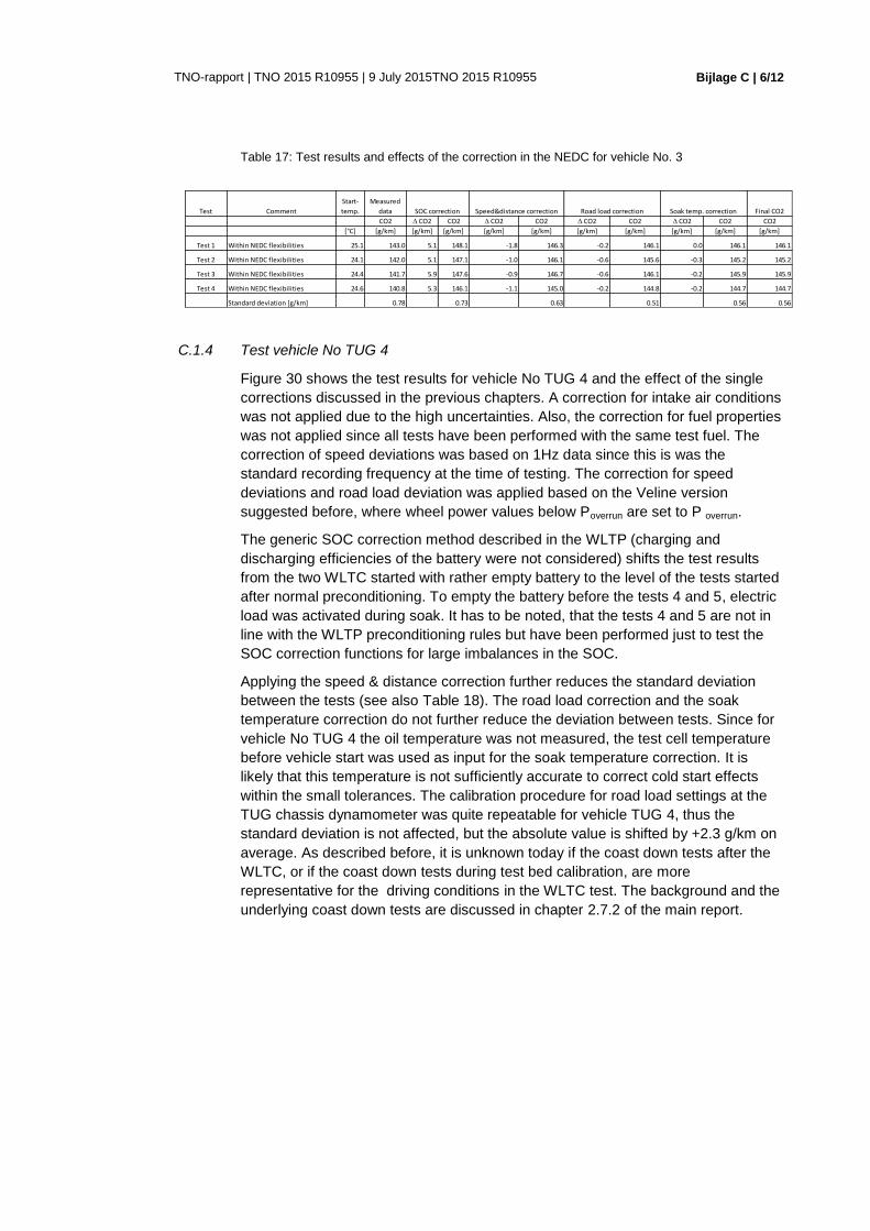
Bijlage C | 6/12
TNO-rapport | TNO 2015 R10955 | 9 July 2015TNO 2015 R10955
Table 17: Test results and effects of the correction in the NEDC for vehicle No. 3
C.1.4 Test vehicle No TUG 4
Figure 30 shows the test results for vehicle No TUG 4 and the effect of the single
corrections discussed in the previous chapters. A correction for intake air conditions
was not applied due to the high uncertainties. Also, the correction for fuel properties
was not applied since all tests have been performed with the same test fuel. The
correction of speed deviations was based on 1Hz data since this is was the
standard recording frequency at the time of testing. The correction for speed
deviations and road load deviation was applied based on the Veline version
suggested before, where wheel power values below Poverrun are set to P overrun.
The generic SOC correction method described in the WLTP (charging and
discharging efficiencies of the battery were not considered) shifts the test results
from the two WLTC started with rather empty battery to the level of the tests started
after normal preconditioning. To empty the battery before the tests 4 and 5, electric
load was activated during soak. It has to be noted, that the tests 4 and 5 are not in
line with the WLTP preconditioning rules but have been performed just to test the
SOC correction functions for large imbalances in the SOC.
Applying the speed & distance correction further reduces the standard deviation
between the tests (see also Table 18). The road load correction and the soak
temperature correction do not further reduce the deviation between tests. Since for
vehicle No TUG 4 the oil temperature was not measured, the test cell temperature
before vehicle start was used as input for the soak temperature correction. It is
likely that this temperature is not sufficiently accurate to correct cold start effects
within the small tolerances. The calibration procedure for road load settings at the
TUG chassis dynamometer was quite repeatable for vehicle TUG 4, thus the
standard deviation is not affected, but the absolute value is shifted by +2.3 g/km on
average. As described before, it is unknown today if the coast down tests after the
WLTC, or if the coast down tests during test bed calibration, are more
representative for the driving conditions in the WLTC test. The background and the
underlying coast down tests are discussed in chapter 2.7.2 of the main report.
Test Comment
Start-
temp.
Measured
data Final CO2
CO2 CO2 CO2 CO2 CO2 CO2 CO2 CO2 CO2 CO2
[°C] [g/km] [g/km] [g/km] [g/km] [g/km] [g/km] [g/km] [g/km] [g/km] [g/km]
Test 1 Within NEDC flexibilities 25.1 143.0 5.1 148.1 -1.8 146.3 -0.2 146.1 0.0 146.1 146.1
Test 2 Within NEDC flexibilities 24.1 142.0 5.1 147.1 -1.0 146.1 -0.6 145.6 -0.3 145.2 145.2
Test 3 Within NEDC flexibilities 24.4 141.7 5.9 147.6 -0.9 146.7 -0.6 146.1 -0.2 145.9 145.9
Test 4 Within NEDC flexibilities 24.6 140.8 5.3 146.1 -1.1 145.0 -0.2 144.8 -0.2 144.7 144.7
Standard deviation [g/km] 0.78 0.73 0.63 0.51 0.56 0.56
SOC correction Speed&distance correction Road load correction Soak temp. correction
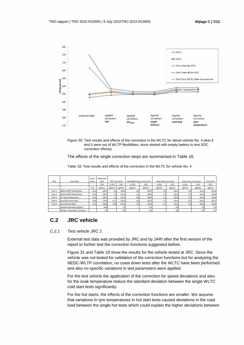
Bijlage C | 7/12
TNO-rapport | TNO 2015 R10955 | 9 July 2015TNO 2015 R10955
Figure 30: Test results and effects of the correction in the WLTC for diesel vehicle No. 4 (test 4
and 5 were out of WLTP flexibilities, since started with empty battery to test SOC
correction effects)
The effects of the single correction steps are summarised in Table 18.
Table 18: Test results and effects of the correction in the WLTC for vehicle No. 4
C.2 JRC vehicle
C.2.1 Test vehicle JRC 1
External test data was provided by JRC and by JARI after the first version of the
report to further test the correction functions suggested before.
Figure 31 and Table 19 show the results for the vehicle tested at JRC. Since the
vehicle was not tested for validation of the correction functions but for analysing the
NEDC-WLTP correlation, no coast down tests after the WLTC have been performed
and also no specific variations in test parameters were applied.
For the test vehicle the application of the correction for speed deviations and also
for the soak temperature reduce the standard deviation between the single WLTC
cold start tests significantly.
For the hot starts, the effects of the correction functions are smaller. We assume
that variations in tyre temperatures in hot start tests caused deviations in the road
load between the single hot tests which could explain the higher deviations between
Test Comment
Start-
temp.
Measured
data Final CO2
CO2 CO2 CO2 CO2 CO2 CO2 CO2 CO2 CO2 CO2
[°C] [g/km] [g/km] [g/km] [g/km] [g/km] [g/km] [g/km] [g/km] [g/km] [g/km]
Test 1 Within WLTP flexibilities 23.2 147.9 1.5 149.4 0.3 149.7 1.6 151.3 0.1 151.4 151.4
Test 2 Within WLTP flexibilities 25.4 149.9 1.3 151.2 -1.2 150.0 2.3 152.3 0.7 153.0 153.0
Test 3 19° start temperature 19.3 150.3 1.3 151.6 -0.9 150.7 2.1 152.8 -1.0 151.8 151.8
Test 4 Low SOC at test start 22.8 174.6 -21.1 153.4 -2.0 151.5 2.7 154.1 -0.1 154.1 154.1
Test 5 Low SOC & 2.8 bar 22.4 166.8 -14.9 151.9 -1.4 150.5 2.7 153.2 -0.2 153.0 153.0
Standard deviation [g/km] 10.8 1.3 0.6 0.9 1.0 1.0
Std.dev. from tests 1,2,3 only 1.0 1.0 0.4 0.6 0.7 0.7
SOC correction Speed&distance correction Road load correction Soak temp. correction

Bijlage C | 8/12
TNO-rapport | TNO 2015 R10955 | 9 July 2015TNO 2015 R10955
hot tests compared to the cold tests. However, since no coast downs after the hot
tests have been measured this assumption cannot be validated.
Figure 31: Test results and effects of the correction in the WLTC for diesel vehicle JRC 1
(4 tests are hot starts, 3 tests are cold starts))
The effects of the single correction steps are summarised in Table 19.
Table 19: Test results and effects of the correction in the WLTC for vehicle JRC 1
C.3 JARI vehicles
C.3.1 Test vehicle JARI A
External test data was provided by JRC and by JARI after the first version of the
report to further test the correction functions suggested before.
The tests at JARI included a WLTC with a very aggressive driving style which
frequently accelerated and decelerated within the speed tolerances. This driving
style was reported by JARI as being not at all typical for vehicle chassis
dynamometer tests.
Measured
data Final CO2
CO2 ∆CO2 CO2 ∆CO2 CO2 ∆CO2 CO2 ∆CO2 CO2 CO2
[°C] [g/km] [g/km] [g/km] [g/km] [g/km] [g/km] [g/km] [g/km] [g/km] [g/km]
1 within WLTP flexibilities 25.7 212.85 -0.02 212.83 0.56 213.39 n.a. 213.39 1.04 214.43 214.43
2 within WLTP flexibilities 23.3 217.90 -0.29 217.61 -0.50 217.11 n.a. 217.11 0.10 217.21 217.21
3 within WLTP flexibilities 25.0 215.66 -0.34 215.31 0.07 215.38 n.a. 215.38 0.78 216.16 216.16
2.53 2.39 1.86 1.86 1.40 1.40
Road load corr. Soak temp. corr.
Standard deviation [g/km]
Test Nr. Comments Start Temp.
SOC corr. Speed&distance correction

Bijlage C | 9/12
TNO-rapport | TNO 2015 R10955 | 9 July 2015TNO 2015 R10955
Figure 32: Example for smooth and rough (aggressive) driving style. Source: presentation from
JARI on 10. March 2014
Figure 33 and Table 20 show the results for the single correction steps for vehicle
JARI A. The SOC imbalance was low for this vehicle in all tests, thus the SOC
correction has minor effects. The difference between the normal and the smooth
driving style tests is reduced when the speed and distance correction is applied.
The CO2 value for the aggressive driving style is reduced only if 10Hz speed signals
are used for the correction of speed deviations since the oscillations against the
target speed due to the aggressive driver behaviour were higher than 1Hz.
However, the effect of aggressive driving is by far not completely eliminated by the
correction function. The high difference against the normal test result and the small
cylinder capacity of the test vehicle suggest that the CVT gear box was operating
often in kick-down mode during aggressive driving and thus had on average much
higher engine speeds, which leads to a lower engine efficiency. This effect is
certainly not corrected by the proposed correction methods which only adapt for
differences in the wheel power21
.
Influences of the driving style on the gear selection from automatic transmission
systems in general can hardly be corrected in the type approval process.
For such effects additional criteria for valid tests, based on the driving indexes as
defined in SAE J2951 and as presented by JARI on 10. March 2014 in a meeting
arranged by the Commission, seem to be helpful to eliminate improper driver
behaviour.
21 The correction works better for aggressive driving with test vehicle JARI C, which has a manual
transmission.

Bijlage C | 10/12
TNO-rapport | TNO 2015 R10955 | 9 July 2015TNO 2015 R10955
Figure 33: Test results and effects of the correction in the WLTC for diesel vehicle JARI A
The effects of the single correction steps are summarised in Table 20.
Table 20: Test results and effects of the correction in the WLTC for vehicle JARI A (absolute
values for test results have to be masked for the vehicle)
C.3.2 Test vehicle JARI B
External test data was provided by JRC and by JARI after the first version of the
report to further test the correction functions suggested before.
The effects for test vehicle JARI B are very similar to vehicle JARI A (Figure 34 and
Table 21). The SOC imbalance was also low for this vehicle in all tests, thus the
SOC correction has minor effects. The difference between the normal and the
smooth driving style tests is also reduced when the speed and distance correction
is applied. The CO2 value for the aggressive driving style is reduced only if 10Hz
speed signals are used for the correction of speed deviations since the oscillations
against the target speed due to the aggressive driver behaviour were higher than
Measured
data Final CO2
CO2 ∆CO2 CO2 ∆CO2 CO2 ∆CO2 CO2 ∆CO2 CO2 CO2
[°C] [g/km] [g/km] [g/km] [g/km] [g/km] [g/km] [g/km] [g/km] [g/km] [g/km]
1
within WLTP flexibilities
normal driving 24.2 132.67 0.06 132.73 0.99 133.72 n.a. 133.72 0.28 134.00 134.00
2
within WLTP flexibilities
smooth driving 23.8 128.20 0.07 128.28 2.45 130.73 n.a. 130.73 0.18 130.91 130.91
3
within WLTP flexibilities
aggressive driving 23.1 182.32 0.05 182.37 0.07 182.44 n.a. 182.44 0.04 182.48 182.48
4
within WLTP flexibilities
aggressive driving
10Hz data used for calculations 23.1 182.32 0.04 182.36 -4.08 178.28 n.a. 178.28 0.04 178.32 178.32
30.04 30.02 26.63 29.03 26.53 26.53
3.16 3.15 2.12 28.73 2.18 2.18
Road load corr. Soak temp. corr.
Standard deviation tests 1, 2, 4 [g/km]
Standard deviation tests 1 and 2
Test Nr. Comments Start
Temp. SOC corr. Speed & distance corr.

Bijlage C | 11/12
TNO-rapport | TNO 2015 R10955 | 9 July 2015TNO 2015 R10955
1Hz. Also, for test vehicle JARI B the effect of rough driving is by far not completely
eliminated by the correction function. Again we assume that it was mainly the CVT
that caused differences in the engine speed under rough driving conditions
compared to normal driving. This effect is certainly not corrected by the proposed
correction methods, which only adapt for differences in the wheel power.
The results for the two vehicles with CVT transmission and rather small engines
suggest implementing additional criteria for valid tests based on the driving indexes
as defined in SAE J2951 and as presented by JARI on 10. March 2014.
Figure 34: Test results and effects of the correction in the WLTC for diesel vehicle JARI B
The effects of the correction steps are summarised in Table 21.
Table 21: Test results and effects of the correction in the WLTC for vehicle JARI B (absolute
values for test results have to be masked for the vehicle)
Measured data Final CO2
CO2 ∆CO2 CO2 ∆CO2 CO2 ∆CO2 CO2 ∆CO2 CO2 CO2
[°C] [g/km] [g/km] [g/km] [g/km] [g/km] [g/km] [g/km] [g/km] [g/km] [g/km]
1
within WLTP flexibilities
normal driving 22.5 117.50 0.10 117.60 0.44 118.05 n.a. 118.05 -0.11 117.93 117.93
2
within WLTP flexibilities
smooth driving 25.8 114.40 -0.39 114.01 2.19 116.21 n.a. 116.21 0.59 116.80 116.80
3
within WLTP flexibilities
aggressive driving 23.1 136.94 0.08 137.03 -0.28 136.74 n.a. 136.74 0.03 136.77 136.77
4
within WLTP flexibilities
aggressive driving
10Hz data used for calculations 23.1 136.94 0.07 137.01 -2.51 134.50 n.a. 134.50 0.03 134.53 134.53
12.22 12.37 10.07 10.07 9.93 9.93
2.19 2.54 1.30 11.26 0.80 0.80
Road load corr. Soak temp. corr.
Standard deviation tests 1,2,4 [g/km]
Standard deviation tests 1 and 2
Test Nr. Comments Start Temp. SOC corr. Speed & distance corr.

Bijlage C | 12/12
TNO-rapport | TNO 2015 R10955 | 9 July 2015TNO 2015 R10955
C.3.3 Test vehicle JARI C
In contrary to test vehicles JARI A and JARI B the vehicle JARI C has a manual
transmission system. Figure 35 and Table 22 show the results for the correction
functions for the vehicle C. The SOC imbalance was also low for this vehicle in all
tests, thus the SOC correction has minor effects. For the vehicle C with manual
transmission the difference between all driving styles is eliminated to a large extent
when the speed and distance correction is applied on a 10Hz basis. This effect
shows that differences in the wheel power are efficiently corrected by the proposed
method and that the deviations remaining for vehicle A and B as shown before are
most likely a result from the CVT behaviour.
A correction of speed deviations based on 1Hz signals has almost no effect since
the oscillations against the target speed due to the aggressive driver behaviour
were higher than 1Hz. This suggests demanding a minimum frequency for the
recorded vehicle speed of approximately 5 Hz. Eliminating eventual noise in the
signal needs to be discussed before an eventual implementation into the WLTP.
Figure 35: Test results and effects of the correction in the WLTC for diesel vehicle JARI C
The effects of the correction steps are summarised in Table 22.
Table 22: Test results and effects of the correction in the WLTC for vehicle JARI C (absolute
values for test results have to be masked for the vehicle)
Measured
data Final CO2
CO2 ∆CO2 CO2 ∆CO2 CO2 ∆CO2 CO2 ∆CO2 CO2 CO2
[°C] [g/km] [g/km] [g/km] [g/km] [g/km] [g/km] [g/km] [g/km] [g/km] [g/km]
1
within WLTP flexibilities
normal driving 25.8 179.43 -0.18 179.25 0.62 179.87 n.a. 179.87 0.89 180.77 180.77
2
within WLTP flexibilities
smooth driving 24.3 177.53 -0.15 177.38 1.64 179.02 n.a. 179.02 0.43 179.45 179.45
3
within WLTP flexibilities
aggressive driving 26.1 189.47 -0.23 189.24 0.00 189.25 n.a. 189.25 1.05 190.29 190.29
4
within WLTP flexibilities
aggressive driving
10Hz data used for calculations 26.1 189.47 -0.25 189.23 -8.13 181.09 n.a. 181.09 1.00 182.09 182.09
6.42 6.37 1.04 5.67 1.32 1.32
1.34 1.33 0.60 5.41 0.93 0.93
Road load corr. Soak temp. corr.
Standard deviation tests 1,2,4 [g/km]
Standard deviation tests 1 and 2
Test Nr. Comments Start
Temp. SOC corr. Speed & distance corr.
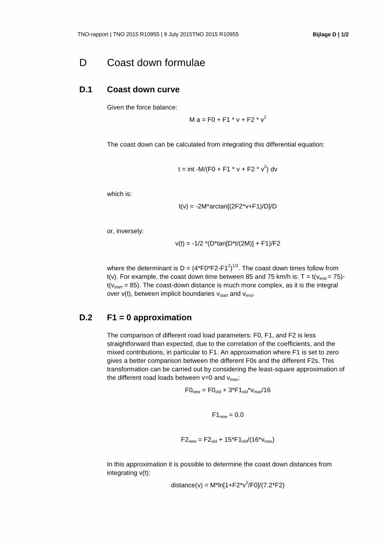
Bijlage D | 1/2
TNO-rapport | TNO 2015 R10955 | 9 July 2015TNO 2015 R10955
D Coast down formulae
D.1 Coast down curve
Given the force balance:
M a = F0 + F1 * v + F2 * v2
The coast down can be calculated from integrating this differential equation:
t = int -M/(F0 + F1 * v + F2 * v2) dv
which is:
t(v) = -2M*arctan[(2F2*v+F1)/D]/D
or, inversely:
v(t) = -1/2 *(D*tan[D*t/(2M)] + F1)/F2
where the determinant is D = (4*F0*F2-F12)1/2
. The coast down times follow from
t(v). For example, the coast down time between 85 and 75 km/h is: T = t(vend = 75)-
t(vstart = 85). The coast-down distance is much more complex, as it is the integral
over v(t), between implicit boundaries vstart and vend.
D.2 F1 = 0 approximation
The comparison of different road load parameters: F0, F1, and F2 is less
straightforward than expected, due to the correlation of the coefficients, and the
mixed contributions, in particular to F1. An approximation where F1 is set to zero
gives a better comparison between the different F0s and the different F2s. This
transformation can be carried out by considering the least-square approximation of
the different road loads between v=0 and vmax:
F0new = F0old + 3*F1old*vmax/16
F1new = 0.0
F2new = F2old + 15*F1old/(16*vmax)
In this approximation it is possible to determine the coast down distances from
integrating v(t):
distance(v) = M*ln[1+F2*v2/F0]/(7.2*F2)

Bijlage D | 2/2
TNO-rapport | TNO 2015 R10955 | 9 July 2015TNO 2015 R10955
The distance is related to the force through the change in kinetic energy:
F = M*(vstart2 – vend
2)/(25.92*distance)
where M is the total vehicle inertia including the rotational inertia. This
approximation is used in the example regarding road slope.

Bijlage E | 1/4
TNO-rapport | TNO 2015 R10955 | 9 July 2015TNO 2015 R10955
E Coast-down validation
In order to establish the correctness and accuracy of the existing and proposed
corrections an extensive test program has been executed. One common vehicle
has been tested on three different circuits, with two types of wheels (standard and
sport) and three types of tyres for those wheels (premium and eco for the normal
wheel, and a sport tyre for the sport wheel). The tests have all been executed
according the protocol described in the WLTP 1a text (UN ECE, 2014). As well as
different wheels, different weights and tyre pressures were also used. The tests are
described in a separate Appendix F In this appendix to the main report only the
main observations are repeated.
In total, 58 hours of test data were collected. The typical spread in coast down
values, expressed at 1/T in consecutive “a” tests, and consecutive “b” tests was
2.8%. For a large part this can be attributed to the variation of the wind during the
test. The total variation with the different conditions was much larger. The size of
each effect is reported below. It must be noted however, that given a test by test
variation of 2.8%, to be on the safe side a similar error margin can be applied to the
results,. The successive tests will reduce the overall error of the tests, however,
2.8% must be considered “unexplained”, i.e., non-reproducible. Very likely, the wind
gustiness plays an important role in this variation in the test results.
Hence the analysis consisted of three phases:
1. Multi-regression analysis on all the data per velocity range. From this
analysis the appropriateness (functional form and magnitude) of the
existing WLTP corrections were determined.
2. Multi-regression analysis on all the data with the functional form a + b*v +
c*v2. From this the magnitude of the effects was determined.
3. Multi-regression analysis on all the data, for the functional form, with the
corrections for wind, temperature, air pressure, road gradient, vehicle
weight, from the magnitude of the remaining effects were determined.
As much as possible all the data was included in the analysis. For example, the
effect of tyre pressure is based on all the data, allowing for offsets for the alternative
tyres (sport and eco):
F0 = F0base + F0pressure-dependence*p + F0sport + F0eco
In this manner all the coast-down data is fitted in a multi-regression analysis
combined with all other effects, like wind and temperature, with four tyre
coefficients: the base value, the dependence on pressure, and offsets for the two
alternative tyres.
The statistical noise is significant for the separate effects within the range of the
WLTP test protocol. Physical arguments, underlying the effects on road load,
should augment the measurement program in order to arrive at proper conclusions
and correction algorithms.

Bijlage E | 2/4
TNO-rapport | TNO 2015 R10955 | 9 July 2015TNO 2015 R10955
E.1 WLTP corrections
The corrections described in the WLTP text have been validated. Overall the
corrections are appropriate, as the same results were found within the bandwidth of
the accuracy:
Test mass correction in the WLTP is somewhat smaller than is seen in the test.
The rolling resistance increased more than proportional with the vehicle weight
with the increase in test mass. This is probably due to the low tyre pressure
prescribed in the vehicle door label.
The stationary wind correction is correct, it reduces the difference between the
“a” and “b” test significantly, in cases of wind above 2.5 m/s.
The temperature correction of the tyres (rubber viscoelasticity) was deemed
correct by the measurement program, despite the complexity of heat transfer
around the tyre.
The need for an air pressure correction is confirmed by the test program. This
air pressure correction is appropriate.
The new approach to average the reciprocal of the coast-down time ensures the
limited contribution of the road slope to the road load results.
The coast-down results were corrected with the WLTP correction methods, for
weight, temperature, and air pressure. The other effects were studied with the
corrected coast down results.
Initially, for each velocity, the analysis was performed separately. The appropriate
velocity dependencies arose in this analysis: constant terms for rolling resistance;
quadratic terms for air drag; and a combination of a constant and a linear term for
wind. Some effects affect only the rolling resistance and yield the same additional
force for all velocities, other effects are related to air drag, and they yield an
additional force that increases with velocity.
In the second stage, the appropriate velocity dependency was inserted for each of
the elements in the test matrix, and the effect was quantified. This yields the most
significant magnitude of each of the variation.
E.2 Consistent effects as observed
In the data, apart from the effects already corrected for in the WLTP text, other
effects can be recognized.
Road surface
The road surface has a significant contribution to the rolling resistance. The road
surface has a significant contribution to the rolling resistance. once all other
corrections were applied to the reference coast down. There was a 20% deviation
between the coast-down tests conducted at the different test tracks. Excluding other
effects, it is likely a greater part of this difference can be attributed to the road
surface.
E.2.1 Grill vanes
The tests were executed with open grill vanes. Only in one test were the grill vanes
closed to study the effect of the air flow through the radiator. The effect on the air

Bijlage E | 3/4
TNO-rapport | TNO 2015 R10955 | 9 July 2015TNO 2015 R10955
drag of open grill vanes is 10%. Not all vehicle models have such grill vanes, and
the setting can vary during driving. However it is unlikely that grill vanes will be
closed during driving, due to the heat from the engine.. Hence, an open grill is an
appropriate approximation to the worst case, and to the real world, settings, which
may be partially closed in some cases.
E.2.2 Aerodynamic options
In one test sequence the vehicle was tested with the kerb-side mirror removed, the
driver-side mirror folded, the antenna and windscreen wiper blades removed, and
the wheel caps taped closed, to approximate a closed wheel. This combination of
factors together yielded a reduction of the air drag of 4%.
E.2.3 Tyre pressure
The effect of tyre pressure turned out to be a complex problem. During the testing,
tyre pressure was monitored and a large variation was found. Rather than relying
on the initial tyre pressure only and the variations therein, the data from the tyre
pressure monitoring was used. The standard tyres have a pressure of 2.1 bar. After
conditioning the pressure was around 2.3 bar. In the case of higher initial pressures,
the pressure after conditioning was also higher, albeit slightly less than in the case
of the 2.1 bar. The variation of the rolling resistance with the monitor pressure was:
F0 = 157 N + 51 N/bar ~ 75 * (2.1 + 0.7/bar)
Using the conditioning pressure of 2.1 bar, the correction of the rolling resistance,
based on this measurement program, would be:
F0road-load = F0test (ptest/pset)0.7
Instead of the exponent of 0.7, exponents of 1 and 1.5 are often quoted in the older
literature. Tyre manufacturers report nowadays an effect corresponding with
exponents from 0.5 to 0.7. The result will depend on the tyre type, and the initial
pressure.
E.2.4 Different tyres and wheels
The vehicle was also tested with sport tyres (18”) which are wider than standard
issue 16” tyres. Compared to the standard tyres the rolling resistance of the sports
tyres was 5% lower, the air drag was 1.5% higher, the latter lying within the margin
of error. The test was not corrected for the substantial high rotational inertia of these
wheels and tyres. This has an effect of an 1% underestimation of the road load
values.
The coast down tests were also conducted with eco-tyres which have a higher set
pressure of 2.7 bar instead of 2.1 bar. For the same pressure, the rolling resistance
of the eco-tyre would have been 9% higher, however, is the higher advised
pressure resulted in 22% reduction in rolling resistance with the pressure, yielding
a net reduction of 13% in rolling resistance for the eco-tyre.
E.2.5 Relative humidity
The effect of relative humidity yields a consistent effect over all the tests, despite
the limited temperatures, between 10o C and 25
o C. The higher relative humidity
yields lower air drag, in the order of the expected result of around one percent.

Bijlage E | 4/4
TNO-rapport | TNO 2015 R10955 | 9 July 2015TNO 2015 R10955
E.2.6 Alignment
Most tests on the vehicle were carried out with the nominal toe-in of the wheels of
0.2o. The wheels are not adjustable in the other directions, e.g. camber and caster.
The vehicle was also tested with a toe-in of 0o. This gives a reduction of rolling
resistance of 6% with respect to the nominal, or midpoint, value.
E.2.7 Road slope
From the GPS data the road slope could be determined. This yields a correction on
the coast-down time. In the WLTP the solution is the use of the average of both
directions. However, it is possible to correct for each direction separately. In this
case the vehicle weight can be recovered, as the additional force is the result of
gravity, vehicle mass, and slope. In this manner only part of the vehicle mass is
recovered.
E.2.8 Curved trajectories
The accuracy of the GPS allowed for the study of a curved trajectory rather than a
straight one. Given the substantial effect of alignment of the wheels, the curved
track can affect the rolling resistance positively. Indeed, given typical deviations of
0.5-1.0 metres from the original endpoint over 100 metres, the larger deviations
give a slightly smaller rolling resistance. There is insufficient data to see a different
effect in the case of 0o alignment.
E.2.9 Wind
The test track in The Netherlands was a few kilometers from the North-Sea coast,
with substantial wind. The meteorological station at the height of 10 meters has an
average wind velocities (measured over the last 10 minutes of the hour and over
the whole hour in the period 2001-2010) of 4.6 m/s, with standard deviations over
an hour and over ten minutes of 2.7 m/s and 2.8 m/s respectively. The same data
also recorded the maximal wind speed (i.e., gusts) during an hour. The average
gust speed is 7.8 m/s. Hence the wind gusts are typically 2.0 m/s higher than the
hourly and ten-minute averages. This is the case for all average velocities, except
the lowest velocities, smaller than 1.0 m/s.
Hence it can be concluded that wind gusts occur at small time scales of seconds,
as there is hardly a distinction between hourly and ten-minute averages.
Furthermore, at this location wind gusts are substantially higher than the average
wind speed.
Comparing the meteorological station with the anenometer (direction and speed) at
the track side, at a height of 0.7 metres above the terrain, the hourly wind
measurement at 10 metres height are 1.5-2.0 m/s higher. In particular, at low wind
speeds the difference is in the top of the range, while at higher wind speeds the
difference is at the bottom of this range. Likewise, the wind gusts at 0.7 metres are
still substantially higher than the average wind speeds, with more than 1.0 m/s
difference.
Hence the wind gusts at track level of 1.0 m/s can explain very well the variations in
the coast down results, from test to test. The test-to-test variation is 2.8%. With a
wind speed difference of 1.0 m/s, i.e., 3.6 km/hr, the 5% variation in the apparent
velocity at 72 km/h matches well with 3% variation in coast-down times.

Bijlage F | 1/26
TNO-rapport | TNO 2015 R10955 | 9 July 2015TNO 2015 R10955
F Coast-down test program
The road load of a vehicle is determined by means of a coast down test. As a large
number of parameters and external conditions influence the coast down test, the
type approval procedures for performing the coast down test allow for certain
margins within which certain test parameters should lie. These margins can partly
explain the difference between the real-world and type approval CO2 emissions.
The main objective of the overall project (WLTP correction algorithms) is to develop
correction factors for various variables in the coast down and chassis dynamometer
test. In order to develop correction factors for the coast down test, TNO investigated
the effect of variations in test parameters during the execution of a coast down test
on the vehicle’s road load by performing a series of coast down measurements.
This appendix describes how the measurements were performed, chassis
dynamometer results are not described in this report.
Variations on the following factors were identified and investigated:
1. Rolling resistance and inertia: tyre pressure, fitted tyres, wheel alignment,
wheel size, test mass;
2. Air resistance: grill vane settings, type of rims, removal of certain accessories
such as antennas, passenger side mirrors, etc;
3. Ambient conditions: temperature, wind speed, wind direction, atmospheric
pressure, relative humidity;
4. Road properties: road surface, road gradient.
In order to ensure representative test results, TNO selected a vehicle for the
measurements that was within the 2012-2013 top-five of EU sales lists. The vehicle
was equipped with a manual gearbox and was in its original condition.
TNO performed a total of 25 coast down tests, resulting in over 600 runs and 58
hours of data. The tests were performed on three different test tracks in Spain,
Belgium and the Netherlands. TNO used the same equipment for each test to
obtain reliable and comparable data. Furthermore the same weather station, tyre
pressure gauge, temperature gauge and weighing scales were used on each test
track.
To ensure accurate measurements TNO established a fixed procedure for vehicle
preparation, vehicle warm-up, execution of the test and post-test checks.
Key issues for this procedure are:
Following the procedure in accordance with the Draft WLTP GTR, Annex 4;
Checking tyre pressure and tyre temperature before, during and after the test;
Weighing of the vehicle before and after the test;
Performing a minimum of 12 test runs in both directions per test;
Making sure the starting position on test track was similar for each test
Bijlage F | 2/26
TNO-rapport | TNO 2015 R10955 | 9 July 2015TNO 2015 R10955
F.1 Background
Real-world CO2 emissions of passenger cars very often deviate from the type
approval value. The type approval value for CO2 emissions of passenger cars is
based on a chassis dynamometer test in a laboratory. The total vehicle resistance
of a vehicle, or ‘road load’, is simulated on the chassis dynamometer to obtain
representative emissions.
The road load of a vehicle is determined by means of a coast down test. A coast
down test is performed on an outside test track by coasting the vehicle down from
125 km/h to 15 km/h with the gearbox in neutral position. To improve the accuracy
of the test, the test is performed multiple times in both directions. Speed and time
are measured very accurate during the coast down test. Because the weight of the
vehicle is known, the resistance curve of the vehicle can be determined.
As a large number of parameters and external conditions influence the coast down
test, the type approval procedures for performing the coast down test allow for
certain margins within which certain test parameters should lie. These margins can
partly explain the difference between the real-world and type approval CO2
emissions.
F.2 Aim and approach
The main objective of the overall project (WLTP correction algorithms) is to develop
correction factors, for important flexibilities found, for various variables in the coast
down and chassis dynamometer test. In order to develop correction factors for the
coast down test, TNO investigated the effect of variations in test parameters during
the execution of a coast down test on the vehicle’s road load by performing a series
of coast down measurements. This appendix describes how the measurements
were performed. Chassis dynamometer results are not described in this report.
Variations on the following subjects were identified and investigated:
Rolling resistance and inertia
1. Tyre pressure, fitted tyres, wheel alignment, wheel size, test mass;
Air resistance
1. Grill vane settings, type of rims, removal of certain accessories such as
antennas, passenger side mirrors, etc;
Ambient conditions
1. Temperature, wind speed, wind direction, atmospheric pressure, relative
humidity;
Road properties, road surface, road gradient.
F.3 Structure of this appendix
After the summary and introduction the test method is described in F.2. The test
method gives more info about the used vehicle, tracks, equipment and the test
procedure. F.4 describes the performed measurements programme and gives more
information with regard to the tests undertaken.

Bijlage F | 3/26
TNO-rapport | TNO 2015 R10955 | 9 July 2015TNO 2015 R10955
F.4 Test vehicle
In order to ensure representative test results, TNO selected a vehicle for the
measurements that was within the 2012-2013 top-five of EU sales lists. The vehicle
was equipped with a manual gearbox and was in its original condition. Before
testing, the vehicle was checked at an official dealer to ensure that the vehicle was
in conformity with the manufacturer’s specifications. Also the wheel alignment was
set in the exact middle of the given tolerances and new tyres were fitted and were
run-in for more than 200 km.
Table 23 show the vehicle specifications. With these specifications the vehicle is
suitable for coast down testing according to the Draft WLTP GTR, Annex 4.
Table 23: Test vehicle specifications
Vehicle model Ford
Type Focus, hatchback, 5 doors
Odometer start [km] 27.402
Fuel Gasoline
Construction year 2011
Unladen mass [kg] 1.276
Laden mass [kg] 1.825
Maximum power [kW] 92
Engine capacity [cm3] 1.596
Gearbox Manual
Figure 36: Test vehicle, Ford Focus
F.5 Test tracks
TNO performed a total of 25 coast down tests, the tests were performed on three
different test tracks in the Netherlands (15 tests), Spain (8 tests) and Belgium (2
tests).

Bijlage F | 4/26
TNO-rapport | TNO 2015 R10955 | 9 July 2015TNO 2015 R10955
F.5.1 Air base Valkenburg (Netherlands)
Fifteen coast down tests were performed in the Netherlands. The selected test track
was an airstrip of a closed military air base “Valkenburg” in Katwijk. The airstrip has
a length of ±2,200 metres with asphaltthat has a relatively coarse structure but
which was in good and evenly shape, see Figure 37. At the end, the beginning and
turns of the airstrip the road surface consists of concrete. This concrete road
surface was only used as run-up and turning, not for the measurements. The slope
of the test track is almost zero.
Katwijk is located close to the sea and the test track is open to the wind and does
not have any shelter provided by trees or other obstacles, therefore the wind speed
is more constant, but also on average higher than inland. White lines are located in
the middle of the test track, which are used as aid for driving straight.
A local weather station of the meteorological institute (KNMI) is located about 100
metres next to the test track.The information from this weather station is used as a
back-up.
Measurements on this test track were performed to determine the effect of vehicle
adjustments, atmospheric conditions and road properties. At this track TNO had
exclusive usage for each measurement. Tests were performed during the morning
and afternoon.
Figure 37: The air-strip and asphalt structure at air base Valkenburg

Bijlage F | 5/26
TNO-rapport | TNO 2015 R10955 | 9 July 2015TNO 2015 R10955
Figure 38: The air-strip from above, source: www.airwork.nl. The weather station is visible in the
field right from the track.
F.5.2 IDIADA proving ground (Spain)
Eight coast down tests were performed in Spain at the high speed circuit of IDIADA
proving ground. The high speed circuit is an oval circuit with a total length of ±7,500
metres and has four lanes with even and relatively dense asphalt, see Figure 39
and Figure 40. Each lane has different maximum and minimum speeds. For the
measurements only the straights of the lanes were used. These straights have a
length of ±2,200 metres and a longitudinal gradient of 0.3%, this gradient being in
one direction positive and in the opposite direction negative. The bends were only
used for run-up.
The greater part of the high speed circuit is relatively well sheltered by a hill and/or
trees. Wind speeds can be very low at this circuit.
During the measurements lane 2 was used for the speeds higher than 100 km/h
and lane 1 was used for the speeds lower than 100 km/h. After the lane changing
the vehicle was accelerated again to 10 km/h above the starting speed.
A weather station is located next to the test track.The information from this weather
station is used as a back-up.
Measurements on this test circuit were performed to determine the effect of
atmospheric conditions and road properties. No vehicle adjustments were
conducted during these measurements. There was no exclusive usage of the test
track requested for the measurements. Tests were performed during the morning,
afternoon, evening and night. During the evening, night and early in the morning
very few other cars were present on the test track.
±2200 meters of asphalt
Concrete was only
used for run-up and
turning

Bijlage F | 6/26
TNO-rapport | TNO 2015 R10955 | 9 July 2015TNO 2015 R10955
Figure 39: The high-speed circuit and associated asphalt structure
Figure 40: IDIADA proving ground from above, source: Google Maps
F.5.3 Ford Lommel proving ground (Belgium)
Two coast down tests were performed in Belgium at the “Straight Away” of Ford
Lommel proving ground. The Straight Away’ is a straight track with an usable length
of ±2,300 metres and has two lanes, one lane for each direction, see Figure 41.
Regular asphalt with a common structure is used for the road surface. Before the
beginning of the track some space is available for run-up, measurements were only
performed on the test track.
The greater part of the Straight Away is relatively well sheltered by trees, in addition
Lommel lies far from the sea, therefore wind speeds are often relatively low at this
circuit.
A weather station is located next to the test track.The information from this weather
station is used as a back-up.
Measurements on this test circuit were performed mainly to determine the effect of
road properties. No vehicle adjustments were conducted during these
measurements. No exclusive usage of the test track was requested for the
measurements. However, tests could be performed well. Tests were performed
during the morning and afternoon.
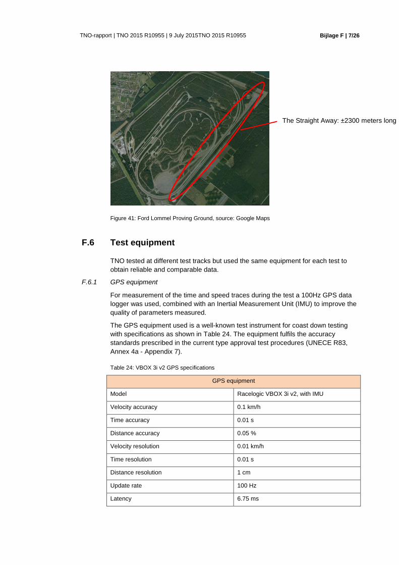
Bijlage F | 7/26
TNO-rapport | TNO 2015 R10955 | 9 July 2015TNO 2015 R10955
Figure 41: Ford Lommel Proving Ground, source: Google Maps
F.6 Test equipment
TNO tested at different test tracks but used the same equipment for each test to
obtain reliable and comparable data.
F.6.1 GPS equipment
For measurement of the time and speed traces during the test a 100Hz GPS data
logger was used, combined with an Inertial Measurement Unit (IMU) to improve the
quality of parameters measured.
The GPS equipment used is a well-known test instrument for coast down testing
with specifications as shown in Table 24. The equipment fulfils the accuracy
standards prescribed in the current type approval test procedures (UNECE R83,
Annex 4a - Appendix 7).
Table 24: VBOX 3i v2 GPS specifications
GPS equipment
Model Racelogic VBOX 3i v2, with IMU
Velocity accuracy 0.1 km/h
Time accuracy 0.01 s
Distance accuracy 0.05 %
Velocity resolution 0.01 km/h
Time resolution 0.01 s
Distance resolution 1 cm
Update rate 100 Hz
Latency 6.75 ms
The Straight Away: ±2300 meters long

Bijlage F | 8/26
TNO-rapport | TNO 2015 R10955 | 9 July 2015TNO 2015 R10955
Figure 42: The VBOX 3i v2 datalogger on the left and the IMU on the right
F.6.2 Monitoring equipment
Besides the GPS equipment the same weather monitoring system, tyre inflator,
handheld thermometer and weighing scales were also used at the different test
tracks for monitoring purposes. Specifications of the monitoring equipment are
shown in Table 25. With these specifications the equipment fulfils the accuracy
standards in the WLTP consolidated draft GTR of August 2, 2013. In Appendix 7 of
the UNECE R.83 these accuracy standards are not prescribed.
Table 25: Specifications of test equipment
Weather monitoring system
Model Davis Vantage Vue, with datalogger
Logging interval 1 minute
Height of the weather station 0.7 meter above the road surface
Wind speed accuracy 5% accuracy
Wind direction accuracy 3° accuracy
Atmospheric temperature accuracy 0.5°C accuracy
Atmospheric pressure accuracy 1.0 mb accuracy
Tyre inflator
Model Förch PCL, hand calibrated
Reading accuracy 1 kPa
Weighing scale
Model Intercomp SW500 cabled scales system
Accuracy 0.1%
# scales 4
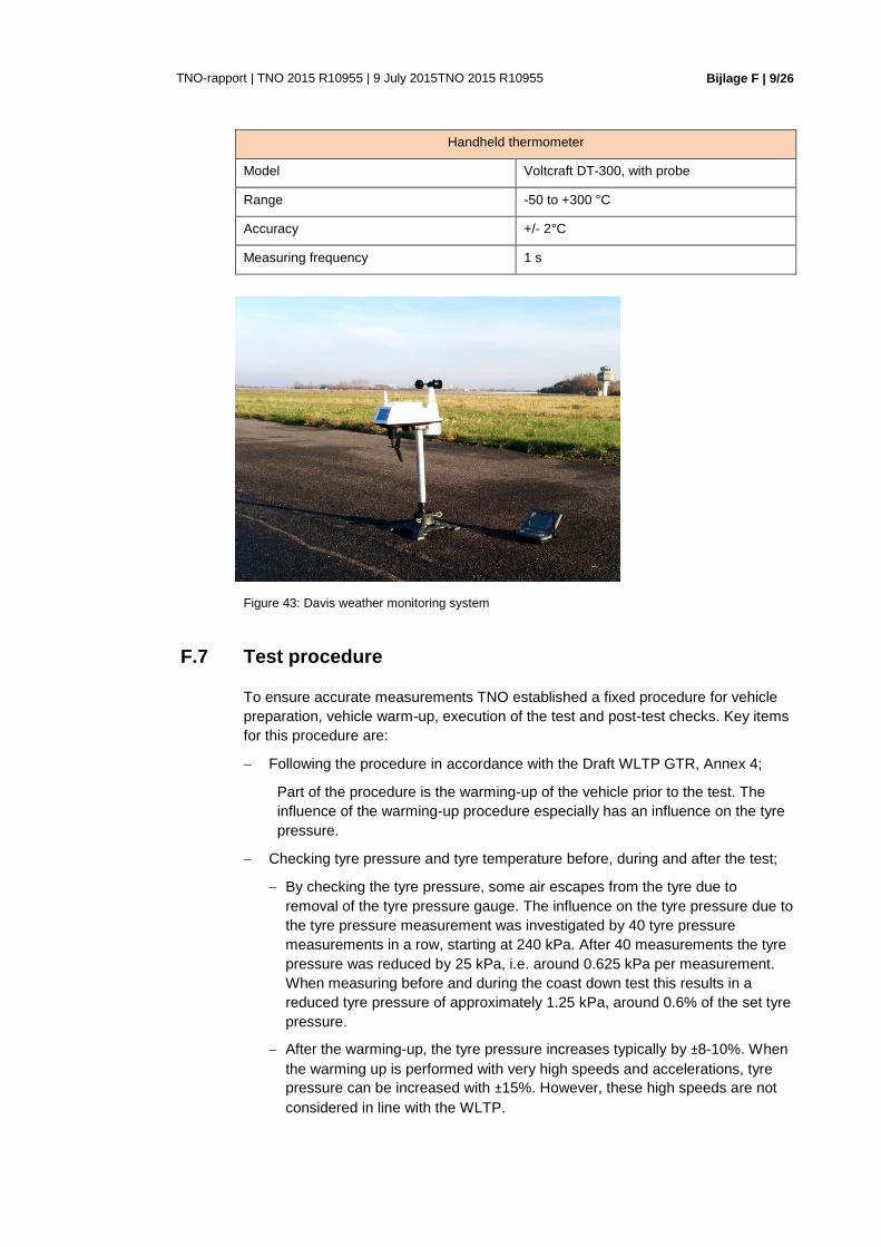
Bijlage F | 9/26
TNO-rapport | TNO 2015 R10955 | 9 July 2015TNO 2015 R10955
Handheld thermometer
Model Voltcraft DT-300, with probe
Range -50 to +300 °C
Accuracy +/- 2°C
Measuring frequency 1 s
Figure 43: Davis weather monitoring system
F.7 Test procedure
To ensure accurate measurements TNO established a fixed procedure for vehicle
preparation, vehicle warm-up, execution of the test and post-test checks. Key items
for this procedure are:
Following the procedure in accordance with the Draft WLTP GTR, Annex 4;
Part of the procedure is the warming-up of the vehicle prior to the test. The
influence of the warming-up procedure especially has an influence on the tyre
pressure.
Checking tyre pressure and tyre temperature before, during and after the test;
By checking the tyre pressure, some air escapes from the tyre due to
removal of the tyre pressure gauge. The influence on the tyre pressure due to
the tyre pressure measurement was investigated by 40 tyre pressure
measurements in a row, starting at 240 kPa. After 40 measurements the tyre
pressure was reduced by 25 kPa, i.e. around 0.625 kPa per measurement.
When measuring before and during the coast down test this results in a
reduced tyre pressure of approximately 1.25 kPa, around 0.6% of the set tyre
pressure.
After the warming-up, the tyre pressure increases typically by ±8-10%. When
the warming up is performed with very high speeds and accelerations, tyre
pressure can be increased with ±15%. However, these high speeds are not
considered in line with the WLTP.
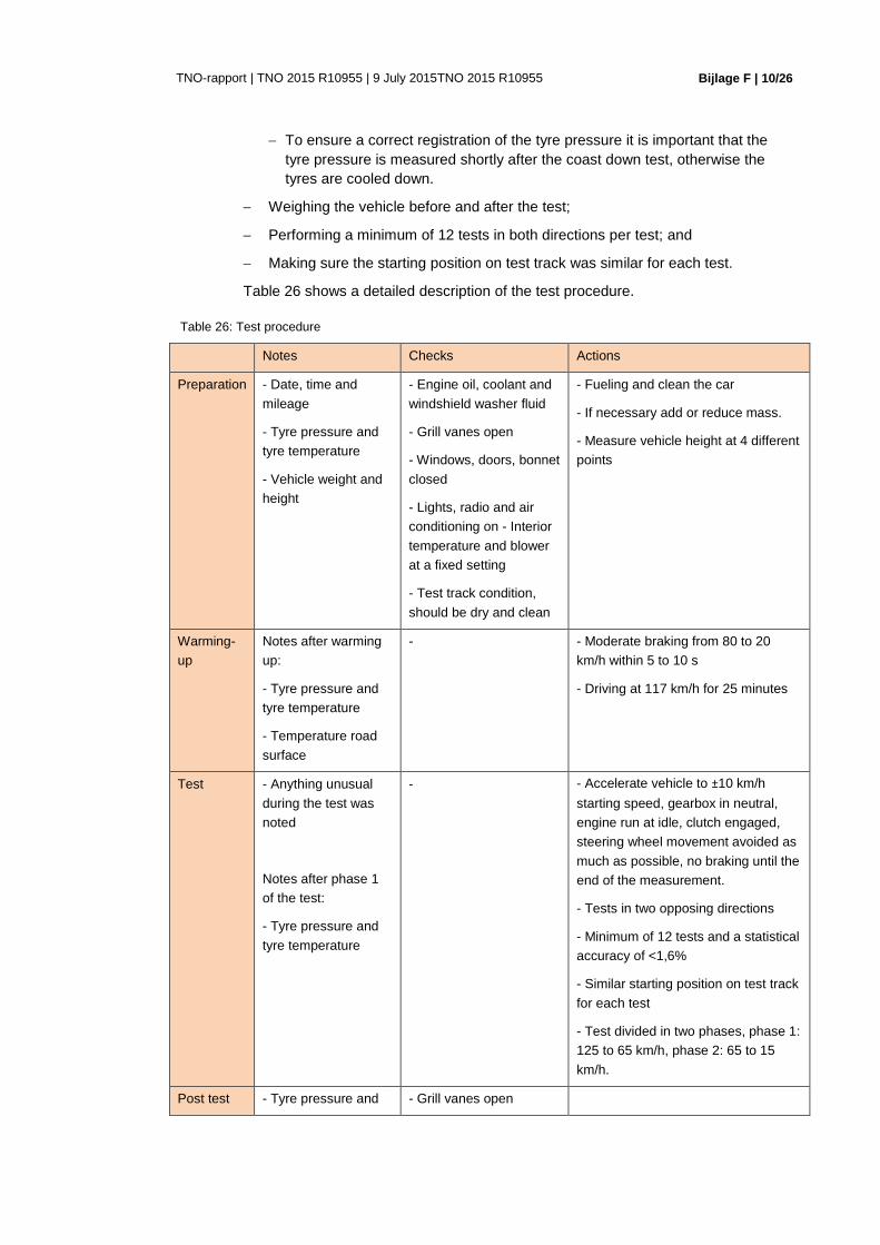
Bijlage F | 10/26
TNO-rapport | TNO 2015 R10955 | 9 July 2015TNO 2015 R10955
To ensure a correct registration of the tyre pressure it is important that the
tyre pressure is measured shortly after the coast down test, otherwise the
tyres are cooled down.
Weighing the vehicle before and after the test;
Performing a minimum of 12 tests in both directions per test; and
Making sure the starting position on test track was similar for each test.
Table 26 shows a detailed description of the test procedure.
Table 26: Test procedure
Phase Notes Checks Actions
Preparation - Date, time and
mileage
- Tyre pressure and
tyre temperature
- Vehicle weight and
height
- Engine oil, coolant and
windshield washer fluid
- Grill vanes open
- Windows, doors, bonnet
closed
- Lights, radio and air
conditioning on - Interior
temperature and blower
at a fixed setting
- Test track condition,
should be dry and clean
- Fueling and clean the car
- If necessary add or reduce mass.
- Measure vehicle height at 4 different
points
Warming-
up
Notes after warming
up:
- Tyre pressure and
tyre temperature
- Temperature road
surface
- - Moderate braking from 80 to 20
km/h within 5 to 10 s
- Driving at 117 km/h for 25 minutes
Test - Anything unusual
during the test was
noted
Notes after phase 1
of the test:
- Tyre pressure and
tyre temperature
- - Accelerate vehicle to ±10 km/h
starting speed, gearbox in neutral,
engine run at idle, clutch engaged,
steering wheel movement avoided as
much as possible, no braking until the
end of the measurement.
- Tests in two opposing directions
- Minimum of 12 tests and a statistical
accuracy of <1,6%
- Similar starting position on test track
for each test
- Test divided in two phases, phase 1:
125 to 65 km/h, phase 2: 65 to 15
km/h.
Post test - Tyre pressure and - Grill vanes open

Bijlage F | 11/26
TNO-rapport | TNO 2015 R10955 | 9 July 2015TNO 2015 R10955
tyre temperature
- Temperature road
surface and
temperature of the
brakes
- Vehicle weight
- Windows, doors, bonnet
closed
F.8 Coast-down measurement program
F.8.1 Test programme
TNO performed a total of 25 coast down tests, resulting in over 600 runs and 58
hours of data. Table 27 show the performed tests divided over the three test tracks.
The table is not in chronological order, the column “Test ID” indicates the test
sequence. During measurements were a vehicle setting was adjusted, only one
type of adjustment was tested at the same time, other settings remained equal to
the reference situation. The following paragraphs describe more details with regard
to the test variations.
Table 27: Measurement programme
Measurement Test track
Valkenburg
Test track
IDIADA
Test track
Ford LPG
Total Test ID
Reference situation
(210 kPa tyre pressure)
4 tests 8 tests 2 tests 14 tests 1-11, 22-24
Tyre pressure at 250 and
290 kPA
2 tests - - 2 tests 12, 13
Eco tyres at
210 kPa and 290 kPa
2 tests - - 2 tests 20, 21
Optimal wheel alignment
(0o)
1 test - - 1 test 25
18 inch sportive rims, with
sport tyres
2 tests - - 2 tests 16, 17
Test mass high and extra
low
2 tests - - 2 tests 14, 15
Grill vanes closed 1 test - - 1 test 18
Optimization on air
resistance
1 test - - 1 test 19
Ambient conditions* 15 tests 8 tests 2 tests 25 tests All
Road properties* 15 tests 8 tests 2 tests 25 tests All
Total 15 tests 8 tests 2 tests 25 tests -
* The effects of ambient conditions and road properties are obtained by using all test data.

Bijlage F | 12/26
TNO-rapport | TNO 2015 R10955 | 9 July 2015TNO 2015 R10955
F.9 Reference situation
With the vehicle in the reference situation (16” wheels, premium tyres, test mass
high, and open grill, nominal wheel aligment (toe in)), tests were performed on three
test tracks. At the ‘Valkenburg’ test track, reference measurements were performed
at the beginning, the middle and at almost the end of the complete measurement
programme.
As a reference situation the vehicle was confirmed the manufacturer’s specifications
at the local dealer garage. Possible variables of the vehicle settings are explained in
more detail in the text below.
Tyre specifications and tyre pressure: New tyres were fitted with the following
specifications: Continental PremiumContact 5, 205/55 R16, fuel economy label C.
Before the test programme was started, the tyres had been run-in for more than 200
kilometres. The tyres were not specially conditioned or treated. The vehicle
manufacturer provided a tyre pressure range between 210 kPa and 290 kPa, for the
reference situation, A tyre pressure of 210 kPa was maintained.
Wheel alignment: The wheel alignment of the vehicle was checked and adjusted
before the start of the testing program. The toe-in and toe-out of the wheels can be
adjusted for both the front and rear wheels. Other typical alignment items, such as
camber and caster can’t be adjusted for this vehicle but were within the tolerances
of the manufacturer’s specifications. The alignment tolerances and values after
adjustments are shown in Table 28:
Table 28: Wheel alignment specifications
Definition Tolerance Nominal
setting
Maximum
deviation left
or right
Setting test vehicle
Front wheels
Total toe 0.0° to 0.4° 0.2° toe-in ±
0.2°
0.19° toe-in, evenly
setting of both wheels
Camber -1.82° to 0.68° -0.57° 1.25° Left: 0.02°
Right: -0.41°
Caster 3.28° to 5.28° 4.28° 1.00° Left: 4.36°
Right: 4.15°
Rear wheels
Total toe 0.18° to 0.58° 0.38° toe-in ±
0.2°
0.37° toe-in, evenly
setting of both wheels
Camber -2.66° to -0.16° -1.41° 1.25° Left: -1.42°
Right: -2.04°
Test mass: The baseline tests and other non-mass related tests were performed
with minimum permissible reference mass, 1443 kg. The calculation parameters
and the determined minimum permissible reference mass are shown in Table 29.

Bijlage F | 13/26
TNO-rapport | TNO 2015 R10955 | 9 July 2015TNO 2015 R10955
To reach the desired test mass, load was added to the passenger seat of the
vehicle.
Table 29: Test masses and associated parameters
Unladen Mass 1276 kg
Laden mass 1825 kg
Standard load (driver and
luggage)
100 kg
Package of options 0 kg
Factor for variable mass 15%
Test mass low* 1443 kg
*Calculated according the Draft WLTP GTR, Annex 4
Grill Vanes: One of the test vehicle’s features are active grill vanes. Most likely the
vanes close partly with a cold engine and the vanes close at high speeds to reduce
the air-resistance.
To avoid untraceable behaviour of the active grill vanes, the grill vanes were forced
and fixed in an open position during the tests. The open position was established at
an official Ford workshop to avoid possible ECU errors.
F.10 Rolling resistance and inertia
F.10.1 Tyre pressure at 250 and 290 kPa
As mentioned earlier, the vehicle manufacturer provided a tyre pressure range
between 210 kPa and 290 kPa. For the reference situation a tyre pressure of 210
kPa was set. To investigate the effect of a higher tyre pressure, tests were
performed at 250 and 290 kPa. Including the reference tests at 210 kPa, three
different tyre pressure settings were tested.
F.10.2 Eco tyres
An “eco” tyre is designed to reduce the rolling resistance. The reference tyres of the
measurements were from Continental. To investigate the effect of an eco-tyre
versus a regular tyre it is important that both tyre types have the same dimensions
and are of the same brand. Also important is that the tyres are off the same
production line, i.e., the production time should not differ a lot.
New tyres were fitted with the following specifications: Continental EcoContact 5,
205/55 R16, fuel economy label B. Before the tests started, the tyres were run-in for
more than 200 kilometres. The tyres were not specially conditioned or treated.
Continental recommends a high tyre pressure for the eco tyres. Tests were
performed with the tyre pressure at 210 kPa and at 290 kPa. With the test at 210
kPa the eco tyre can be compared with the reference situation, knowing that 210
kPa is not recommended for the eco tyre. With the test at 290 kPa the full potential
of the Eco tyre was investigated, also the reference tyres were tested at 290 kPa,

Bijlage F | 14/26
TNO-rapport | TNO 2015 R10955 | 9 July 2015TNO 2015 R10955
hence a good comparison between both tyre types is possible. In addition the effect
of a higher tyre pressure can be analysed again.
After the tests, the reference tyres were fitted again. To minimize the effect of the
wheel exchange, the rims and wheel hubs were marked so that the wheels could be
fitted on the same axle on the same position as before. Furthermore, the
measurements with the eco tyres were planned as test 20 and 21 to minimize
possible effects on the measurement programme.
F.11 Alternative wheel alignment
As mentioned before only the toe-in and toe-out of the wheels can be adjusted for
both the front and rear wheels. To investigate whether a neutral toe is beneficial for
the rolling resistance during a coast down test the front and rear toe was set to 0°,
see Table 30.
It is difficult to position the alignment back to the exact reference position, hence the
test with the zero toe-in setting is performed at the end of the measurement
programme.
Table 30: Toe settings
Definition Tolerance Reference
setting
Test setting
Front wheels:
Total toe
0.0° to 0.4° 0.19° toe-in,
evenly setting
of both wheels
0.0° toe, evenly
setting of both wheels
Rear wheels:
Total toe
0.18° to 0.58° 0.37° toe-in,
evenly setting
of both wheels
0.0° toe, evenly
setting of both wheels
F.11.1 18 inch sportive rims, with sport tyres
The investigation with regard to the 18 inch wheels has a dual purpose. TNO was
interested in the increase in air-resistance due to a very open structure of a rim and
the increase in width of the wheel. On the other hand an expected increase of
inertia force was expected due to the higher weight of the rims.
Sportive rims of the brand “LM” were purchased in combination with 18 inch tyres.
The rims are part of the Ford Focus model range for rims. The rims are made of
alloy and have an open structure, see Figure 44. The reference rims are 16 inch
and made of steel with a wheelcap mounted.
New tyres were fitted with the following specifications: Continental SportContact 5,
235/40 R18, fuel economy label C. Before the tests started, the tyres were run-in for
more than 200 kilometres. The tyres were not specially conditioned or treated.
Table 31 show the weights of the 18 and 16 inch tyres and rims.
Two tests were performed with the 18 inch wheels, both with the reference test
mass. Due to the higher weight of the rims, 17 kg of load was removed. One test
was performed with the tyre pressure at 210 kPa for all wheels. The other test was

Bijlage F | 15/26
TNO-rapport | TNO 2015 R10955 | 9 July 2015TNO 2015 R10955
performed with a tyre pressure of 230 kPa for the front wheels and 210 kPa for the
rear wheels.This is a possible variation for this wheel size for this vehicle model.
Figure 44: Left 18 inch rim, right 16 inch wheel
Table 31: Wheel masses
Type Mass
[kg]
Total 1 wheel
[kg]
Total 4 wheels [kg]
16 inch rims 8.1 17.0 68.1
16 inch tyres 9.0
18 inch rims 11.5 21.3 85.3
18 inch tyres 9.8
Inertia measurements
For determination of the inertia and resistance of the wheels including connected
rotating vehicle parts, extra measurements were performed. The measurements
were performed by a coast down test for each wheel on a vehicle lift. The vehicle lift
was set on the highest position for enough clearance between the wheels and floor.
To bring the wheel up to speed a line with a weight coiled around the wheel was
dropped, see Figure 45. The measurements were performed for both wheel sets,
i.e. the 16 and 18 inch wheels. For each wheel of both wheel sets the measurement
was repeated 10 times to improve the accuracy.
In order to distinguish between the inertia and resistance, two different weights
were used, a 3 kg and a 6 kg weight. As an input for the calculation the wheel
circumference was measured, wheel speed and coasting time was obtained from
the CAN-bus of the vehicle. The wheel speed was calibrated with the same GPS
data logger as used for the coast down measurements on the road.

Bijlage F | 16/26
TNO-rapport | TNO 2015 R10955 | 9 July 2015TNO 2015 R10955
Figure 45: Inertia test
F.12 Test mass high and extra low
To investigate the effect of a higher or lower test mass, two additional test masses
were tested. The determination of the high test mass is based on the WLTP. The
reference mass was already the low test mass according to the WLTP. In order to
test with a lower test mass than the reference, all load was removed from the
vehicle and the fuel tank was only partly filled. To reach the desired high test mass,
load was added equally to the passenger side, luggage compartment and back seat
of the vehicle.
The calculation parameters for the maximum test mass and the determined test
masses are shown in Table 32:
Table 32: Test mass high and extra low including associated parameters
Unladen Mass 1276 kg
Laden mass 1825 kg
Standard load (driver and
luggage)
100 kg
Package of options*** 150 kg
Factor for variable mass 15%
Test mass low* 1443 kg
Test mass high* 1571 kg
Test mass extra low** 1380 kg
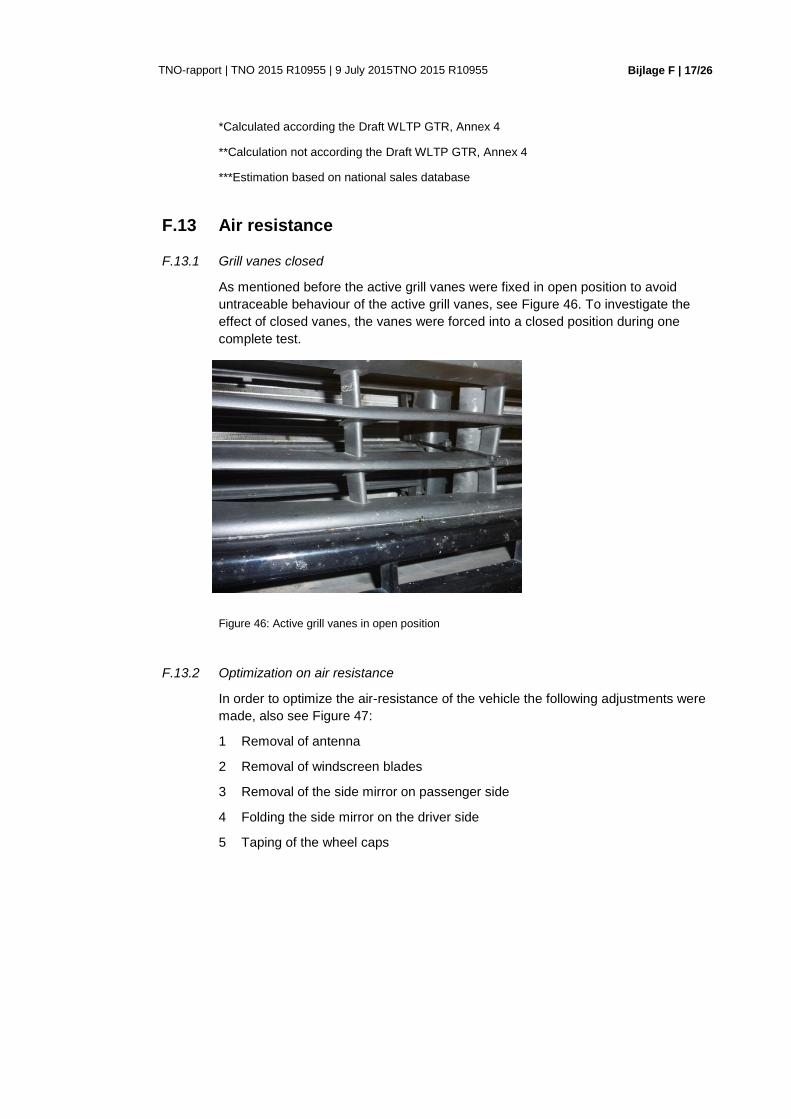
Bijlage F | 17/26
TNO-rapport | TNO 2015 R10955 | 9 July 2015TNO 2015 R10955
*Calculated according the Draft WLTP GTR, Annex 4
**Calculation not according the Draft WLTP GTR, Annex 4
***Estimation based on national sales database
F.13 Air resistance
F.13.1 Grill vanes closed
As mentioned before the active grill vanes were fixed in open position to avoid
untraceable behaviour of the active grill vanes, see Figure 46. To investigate the
effect of closed vanes, the vanes were forced into a closed position during one
complete test.
Figure 46: Active grill vanes in open position
F.13.2 Optimization on air resistance
In order to optimize the air-resistance of the vehicle the following adjustments were
made, also see Figure 47:
1 Removal of antenna
2 Removal of windscreen blades
3 Removal of the side mirror on passenger side
4 Folding the side mirror on the driver side
5 Taping of the wheel caps

Bijlage F | 18/26
TNO-rapport | TNO 2015 R10955 | 9 July 2015TNO 2015 R10955
Figure 47: Optimization for air-resistance
F.14 Ambient conditions and road properties
The effect of ambient conditions and road properties were investigated by using all
available data from all 25 coast down tests. The following parameters were
investigated:
Ambient conditions:
temperature, wind speed, wind direction, atmospheric pressure, relative
humidity.
Road properties:
road surface, road gradient.
Ambient conditions were continuously monitored during all measurements with the
weather monitoring equipment as described in F.6. In addition the local weather
stations are used as back up.
Road gradients shall be obtained from the GPS data. The road surface is not
measured.
Figure 48: Ambient conditions at the Valkenburg air-strip

Bijlage G | 19/26
TNO-rapport | TNO 2015 R10955 | 9 July 2015TNO 2015 R10955
G Suggested WLTP gtr amendments for deviation against target speed and road load calibration
Meaning of different fonts below:
Text in standard black fonts is the text of the original WLTP Phase 1a gtr.
Text in red fonts is new or amended text compared to WLTP Phase 1a gtr.
Text and numbers marked blue are values open for further discussion. Text in italic and blue contains explanations and background information not to be used in
the amendment of the WLTP but to explain the suggested amendments
G.1 Amendments describing the correction for deviations against the target speed
It is suggested to add a paragraph 7 and 8 to Annex 7 as described below.
Annex 7 Calculations
Text for paragraphs 1. to 6. does not need any amendments. In case changes will be made in
paragraph 5, all equations are repeated in the new paragraphs 7 and 8.
7. Correction of CO2 for deviations against the target speed
The target velocity is the velocity according to the applicable WLTC as defined in
Annex 2.
The actual vehicle speed is the velocity measured at the chassis dynamometer and
l shall be measured at a frequency of at least 5 Hz.
Option: For the correction of deviations against the target speed the velocity signal
shall be filtered using the xxx filter method to eliminate noise in the signal. We
cannot assess if filtering is necessary and we cannot elaborate a proposal for a proper filter
method since we do not have any data for the measured velocity in >5Hz with a realistic
noise on the signal. The T4253H filter may be useful and could be tested with data from
different chassis dynamometers to analyse if the filter eliminates possible noise in the signals
without filtering real deviations.
The acceleration shall be calculated as described in paragraph 5 of this Annex.
ai =vi−vi−1
3.6×(ti−ti−1) (51)
ami =vmi−vmi−1
3.6×(ti−ti−1) (52)
where
ai is the target acceleration during time period (i-1) to (i), m/s²;
ami is the measured acceleration during time period (i-1) to (i), m/s²;
vi is the target velocity at time ti, km/h;
vmi is the measured velocity at time ti, km/h;
ti is time, s.

Bijlage G | 20/26
TNO-rapport | TNO 2015 R10955 | 9 July 2015TNO 2015 R10955
The power and the forces at the wheels according to target speed and according to
measured velocity shall be calculated as follows.
Fi = f0 + f1 × (vi+vi−1
2) + f2 ×
(vi+vi−1)2
4+ (1.03 × TM) × ai (53)
Pi = 𝐹𝑖 × (vi+vi−1
3.6×2) (54)
Fmi = f0 + f1 × (vmi+vmi−1
2) + f2 ×
(vmi+vmi−1)2
4+ (1.03 × TM) × ami (53)
Pmi = 𝐹𝑚𝑖 × (vmi+vmi−1
3.6×2) (54)
Where
Pi is the target power during time period (i-1) to (i), W
Pmi is the power during time period (i-1) to (i), W
Fi is the target driving force during time period (i-1) to (i), N
Fmi is the driving force during time period (i-1) to (i), N
vi is the target velocity at time ti km/h;
vmi is the measured velocity at time ti km/h;
TM is the test mass, kg;
ai is the target acceleration during time period (i-1) to (i), m/s²;
ami is the measured acceleration during time period (i-1) to (i), m/s²;
f0, f1, f2 are the road load coefficients for the test vehicle under consideration (TML, TMHor TMind) in N, N/km/h and in N/(km/h)² respectively.
All power values below Poverrun are set to Poverrun to exclude negative power values
not relevant for the fuel flow:
𝑃𝑜𝑣𝑒𝑟𝑟𝑢𝑛 = −𝐷
𝑘𝑣× 0.001 (55)
Where
𝑃𝑜𝑣𝑒𝑟𝑟𝑢𝑛 is the power calculated from the Veline equation according to
chapter 8 with zero CO2 emissions, W
D is the constant from the Veline equation in chapter 8, gCO2/s
kv is the slope of the Veline equation in chapter 8, gCO2/kWs
If Pi < Poverrun then Pi = Poverrun (56)
If Pmi < Poverrun then Pmi = Poverrun (57)
The average power for the target velocity and for the measured velocity is
calculated for the power above Poverrun.
P = ∑Pi
𝑛
tendtstart
(58)
𝑃𝑚 = ∑Pmi
𝑛
tendtstart
(59)

Bijlage G | 21/26
TNO-rapport | TNO 2015 R10955 | 9 July 2015TNO 2015 R10955
Where
P Average power from the target velocity, W
Pm Average power from the measured velocity, W
n number of time steps in the WLTC recording
Then the difference in the positive cycle work values is calculated for the 1800
second test duration.
∆𝑊𝑤ℎ𝑒𝑒𝑙 = 1.8 × (𝑃 − 𝑃𝑚) (60)
Where
∆𝑊𝑤ℎ𝑒𝑒𝑙 is the difference in the cycle work, kWs;
P Average power from the target velocity, W;
Pm Average power from the measured velocity, W.
The vehicle based Veline function is applied to correct for deviations against the
average power from the WLTC target velocity.
∆𝐶𝑂2v = ∆𝑊𝑤ℎ𝑒𝑒𝑙 ∗ kv (61)
Where
∆𝑊𝑤ℎ𝑒𝑒𝑙 is the difference in the cycle work, kWs;
kv is the slope of the Veline equation in chapter 7, g CO2/kWs;
∆CO2v is the correction value for the measured CO2 emissions, g.
The CO2 value corrected for deviations in target speed and for corresponding
deviations against target distance is then
𝑀𝐶𝑂2𝑐𝑜𝑟𝑟=
MCO2 × d + ∆CO2v
23.27
Where
𝑀𝐶𝑂2𝑐𝑜𝑟𝑟 is the mass emission of CO2 corrected for deviations in the
velocity and in the distance, g/km;
d is the distance driven over the corresponding WLTC, km;
MCO2 is the mass emission of CO2 as calculated according to chapter 3.2,
g/km;
∆CO2v is the correction value for the measured CO2 emissions, g.
23.27 is the WLTC target test distance, km.
8. Calculation of the vehicle specific Veline
The vehicle specific Veline is a linear equation calculated from the WLTC test result
for CO2 defining the correlation between CO2 emissions in [g/h] and the average
power at the wheel [kW].
CO2 = kv ×𝑃𝑚
1000+ 𝐷 (62)
where

Bijlage G | 22/26
TNO-rapport | TNO 2015 R10955 | 9 July 2015TNO 2015 R10955
CO2 is the CO2 emission value over a test period in the WLTC with the
average power at the wheel of 𝑃𝑚, g/s;
kv is the slope of the Veline equation, g CO2/kWs;
D is the Constant of the Veline equation, gCO2/s
Pm Average power calculated from the measured velocity as defined in chapter
7 and repeated below, W.
Fmi = f0 + f1 × (vmi+vmi−1
2) + f2 ×
(vmi+vmi−1)2
4+ (1.03 × TM) × ami (63)
Pmi = 𝐹𝑚𝑖 × (vmi+vmi−1
3.6×2) (64)
Where
Pmi is the power during time period (i-1) to (i), W
Fmi is the driving force during time period (i-1) to (i), N
vmi is the measured velocity at time ti km/h;
TM is the test mass, kg;
ami is the measured acceleration during time period (i-1) to (i), m/s²;
f0, f1, f2 are the road load coefficients for the test vehicle under consideration (TML, TMHor TMind) in N, N/km/h and in N/(km/h)² respectively.
The power with zero CO2 emissions in the Veline equation is not known when the Veline equation is calculated the first time and shall be set initially to 2% of the rated engine power. The exact value can be calculated iteratively.
𝑃𝑜𝑣𝑒𝑟𝑟𝑢𝑛−0 = −0.02 × 𝑃𝑟𝑎𝑡𝑒𝑑 (65)
𝑃𝑟𝑎𝑡𝑒𝑑 is the rated power of the engine of the test vehicle, W.
All power values below Poverrun-0 are set to Poverrun-0 to exclude negative power
values not relevant for the fuel flow:
If Pmi < Poverrun then Pmi = Poverrun (66)
𝑃𝑚 = ∑Pmi
𝑛
tendtstart
(59)
Where
Pm Average power from the measured velocity, W;
n number of time steps in the WLTC recording.
The 𝑃𝑚 values shall be computed for the single phases of the WLTC as
well as for the entire WLTC as described in equation (59) for the
corresponding start and end time.
The average measured CO2 mass emissions [g/h] from each phase of
the WLTC shall be correlated to the average 𝑃𝑚 values of the
corresponding phase for the single test phases and for the entire
WLTC.

Bijlage G | 23/26
TNO-rapport | TNO 2015 R10955 | 9 July 2015TNO 2015 R10955
The resulting best-fit line is the Veline equation for the tested vehicle.
The best-fit line shall be computed using the least square deviation
method.
Figure A7/1
Example for the Veline for a LDV from the test results of the 4 WLTC
phases. Pm plotted in kW here.

Bijlage G | 24/26
TNO-rapport | TNO 2015 R10955 | 9 July 2015TNO 2015 R10955
G.2 Amendments in the definition of road load calibration on the chassis dynamometer
The following text is a suggested amendment to the WLTP, Annex 4 “Road load
and dynamometer setting” to eliminate unnecessary flexibilities in the calibration of
the road load as described in the report in chapter 2.7.
The text relates to the WLTP version ECE/TRANS/WP.29/2014/27 from 20.
December 2013. Only paragraphs with suggested amendments are printed below.
Other paragraphs are assumed to be unchanged.
Annex 4 Road load and dynamometer setting
8.1. Chassis dynamometer setting by coastdown method
8.1.2. Coastdown
The coastdown test on the chassis dynamometer shall be performed in accordance
to the procedure given in paragraphs 4.3.1.3.1. and 4.3.1.3.2. of this Annex:
8.1.2.1. Following the vehicle warm-up procedure (paragraph 4.2.4. of this Annex),
and immediately prior to each test measurement, the vehicle shall be
accelerated to 5 km/h above the speed at which the coastdown time
measurement begins (vi + v) and the coastdown shall be started
immediately.
8.1.2.2. The first coast down hast to start immediately after the warm-up procedure.
The time delay between the end of one coast down and the start of the
consecutive coast down shall not exceed 3 minutes.
8.1.2.3. During coastdown, the transmission shall be in neutral, and the engine shall
run at idle. Steering wheel movement shall be avoided and the vehicle
brakes shall not be operated until the speed drops below the lowest relevant velocity (vj − ∆v).
Discussion in WLTP IWG resulted in an adoption of the
following text in WLTP gtr Phase 1b:
“8.1.2. Coastdown
The coastdown test on the chassis dynamometer shall be
performed with the procedure given in paragraphs 8.1.3.2.1.
and 8.1.3.2.2. of this Annex and shall start at latest 120 s
after completion of the warm up procedure. Consecutive
coastdown runs shall be started immediately. At the request
of the manufacturer and with approval of the responsible
authorities, the time between the warm up procedure and
coastdowns using the iterative method may be extended to
ensure a proper vehicle setting for the coastdown. The
manufacturer shall give the responsible authority evidence
for requiring additional time and that chassis dynamometer
load setting parameters (e.g. coolant and/or oil temperature,
force on a dynamometer) are not affected.”

Bijlage G | 25/26
TNO-rapport | TNO 2015 R10955 | 9 July 2015TNO 2015 R10955
Paragraphs in between unchanged
8.1.3. Verification
As described now in WLTP phase 1a, the deviation of the resulting coast down times or
forces against the target values is not limited in the WLTP.
We also do not see an explicit link from the equations for adjustments of road load setting in
Annex 4 - Appendix 2 to “8.1.2. Coastdown” but we assume the coast down tests in 8.1.2
shall be used to provide the data for the adjustments according to Appendix 2.
In any case it should be defined, how much the adjusted road load may deviate against the
target road load values. This seems to be defined in 8.1.3.2. with +/- 10N but this paragraph
is valid only “If the vehicle is accelerated under its own power”. We assume the +/-10N limit
is applicable in all cases. Text and amendments suggested:
The verification has to be performed with the final settings of the chassis
dynamometer after the adjustment of chassis dynamometer load setting described
in 8.1.4 and in appendix 2 to Annex 4 of the WLTP. All coastdown runs for the
verification shall follow the procedure described 8.1.2.
The calculated forces in the specified speed ranges shall be within a tolerance of ±
10 N after a least squares regression of the forces for two consecutive coastdowns
against the target values calculated from the tests in 4.3.
8.1.3.1. The target road load value shall be calculated using the target road load coefficient At, Bt and Ct for each reference speed vj:
Ftj = At + Btvj + Ctvj2
where:
Ftj is the target road load at reference speed vj, N;
vj is the jth reference speed, km/h.
8.1.3.2. For dynamometer load setting, two different methods may be used. If the
vehicle is accelerated by the dynamometer, the methods described in
paragraph 8.1.3.2.1. below shall be used. If the vehicle is accelerated under
its own power the methods in paragraphs 8.1.3.2.1. or 8.1.3.2.2. below shall
be used. The acceleration multiplied by speed shall be approximately 6
m²/sec³.
8.1.3.2.1. Fixed run method
For the fixed-run procedure, the dynamometer software shall automatically
run three coastdowns adjusting the set coefficients for each run using the
difference between the previous run's measured and target coefficients. The
final set coefficients shall be calculated by subtracting the average of the
vehicle coefficients obtained from the last two runs from the target
coefficients. Optionally, a single stabilization coastdown may be performed
before beginning the 2 run averaging sequence.
8.1.3.2.2. Iterative method
The calculated forces in the specified speed ranges shall be within a
tolerance of ± 10 N after a least squares regression of the forces for two
consecutive coastdowns.

Bijlage G | 26/26
TNO-rapport | TNO 2015 R10955 | 9 July 2015TNO 2015 R10955
If an error at any reference speed does not satisfy the criteria of the method
described in this paragraph, paragraph 8.1.4. below shall be used to adjust
the chassis dynamometer load setting.
8.1.4. Adjustment
The chassis dynamometer setting load shall be adjusted in accordance with
the procedure specified in Appendix 2 to this Annex, paragraph 1.
Paragraphs 8.1.2. and 8.1.3. above (including subparagraphs) shall be
repeated.
8.2. Chassis dynamometer load setting using torque meter method
The following effects are assumed.
Torque is measured during constant speed phases in descending order. The longer the
speed is kept constant, the higher the rolling resistance is (cool down of tyres) and thus the
OEM will get lower driving resistances if he uses short constant speed phases (minimum is
defined with 5 seconds in “4.4.2.3. Data collection” in the WLTP). Using short measurement
phases should also lead to results comparable to the coast down method since there also
short durations per speed bin occur (on average approx. 10 seconds per speed bin if v= 5
km/h as suggested in 4.3.1.4.1. in the WLTP (i.e. 120 seconds for coast down from 120 to 20
km/h).
If the constant speed phases are longer on the chassis dyno during calibration than on the
test track, the rolling resistance of the tyres would be higher on the chassis dyno> this would
result in lower additional braking forces from the electric machine of the chassis dyno.
The method should demand that the rolling resistance changes similarly over speed on the
chassis dyno than on the test track. To be comparable to the coast down method short
measurement durations shall be used. To avoid artificial high rolling resistances during the
calibration of the chassis dyno road load, the duration of each speed bin shall be limited to
the duration the speed was measured on the test track.
8.2.3. Verification
The verification has to be performed with the final settings of the chassis
dynamometer after the adjustment of chassis dynamometer load setting described
in 8.2.3.3 and in appendix 2 to Annex 4 of the WLTP.
The torque measurement test on the chassis dynamometer shall be performed with
the procedure defined in 4.4.2.
The torque meter(s) shall be identical to the one(s) used in the preceding road test.
The difference between vj and vj+1 shall be identical to the differences in the tests
performed according to 4.4.2.
The duration each actual speed v_ji is run shall be identical to or lower than the
duration in the tests performed according to 4.4.2.
The forces measured in the specified speed ranges shall be within a tolerance of ±
10 N to the target values from 4.4.2..