India in the Global and Regional Trade: Aggregate and Bilateral Trade Flows and

Determinants of Firms’ Decision to ExportT.N. Srinivasan,

Samuel C. Park, Jr. Professor of EconomicsYale University

Email: t.srinivasan@yale.edu

and

Vani Archana,Fellow

Indian Council for Research on International Economic Relations, New Delhi

Email: varchana@icrier.res.in

January 8, 2008

2

• For nearly four decades since independence in 1947 India followed an industrialization strategy that insulated domestic firms from both competition from imports and from each other with the state playing a dominant role in the economy

• In the mid-eighties there were some hesitant steps away from insulation

• A severe macro-economic and balance of payment crisis in 1991 led to a systemic break from this strategy, opened the economy to import competition and to foreign direct investment, reduced the role of the State and expanded that of the market in the economy

Introduction

3

Introduction(contd)

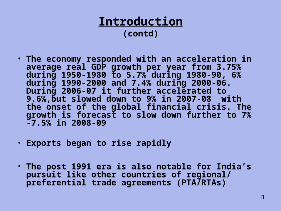
• The economy responded with an acceleration in average real GDP growth per year from 3.75% during 1950-1980 to 5.7% during 1980-90, 6% during 1990-2000 and 7.4% during 2000-06. During 2006-07 it further accelerated to 9.6%,but slowed down to 9% in 2007-08 with the onset of the global financial crisis. The growth is forecast to slow down further to 7% -7.5% in 2008-09

• Exports began to rise rapidly

• The post 1991 era is also notable for India’s pursuit like other countries of regional/ preferential trade agreements (PTA/RTAs)

4

Objectives of the Paper

• To examine the impact of Regional Trade Agreements (RTAs)/Preferential Trade Agreements (PTAs) on India’s trade flows

• To examine the incentive to export of firms in India since 1991

5

Literature Review

• The conclusions from vast empirical literature on the preferential agreements in force have been ambiguous with some finding them to be trade creating and others to be trade diverting

• The literature on gravity models, both theoretical studies and empirical studies, is vast

• Our focus is not on gravity model but on impact of RTAs/ PTAs on India’s bilateral trade flow drawing from the three studies that have a bearing on our model

6

Literature Review • The oldest of the three studies is Soloaga and

Winters (2001), which attempts to estimate the effect on a country’s trade flows of its and its trading partners’ membership (or otherwise) of a PTA

• They find no evidence that recent PTAs boosted intrabloc trade significantly and found trade diversion from the European Union (EU) and European Free Trade Area (EFTA)

• The model we estimate is very close to the following model of Soloaga and Winters

7

where Pki (Pkj) = 1 if country i (j) is a member of the kth PTA (Saloaga and

Winters consider nine PTAs) and zero otherwise

Thus bk measures the intra-bloc effect, i.e., the extent to which bilateral trade is larger than expected when both i and j being members of k,

mk measures the effect of i being a member of k on its imports from j (i.e., exports from j to i ) relative to all countries and

nk is the effect of j being a member of k on its exports to i ( i.e., imports of i from j) relative to all countries

mk and nk combine the effects of general trade liberalization and trade diversion, while bk measures the effect on intra-bloc trade over and above the non-discriminatory trade effect

k ki kj k ki k kjk k k

b P P + m P + n P

8

Adams, et al. (2003)

• Their gravity model is very close to that of Soloaga and Winters

• Their full sample data consists of 116 countries over 28

years (1970-97)

• Their two main findings are: First, of the 18 recent PTA, as many as 12 have diverted more trade from non-members than they have created among members

• Second, these trade diverting PTAs, surprising include the more liberal ones such as EU, NAFTA and MERCOSOUR

9

De Rosa (2007)

• Critically examines the findings of Adams, et al. (2003) using the gravity model of Andrew Rose (2002) and incorporating Soloaga and Winters (2001) dummies for PTA membership

• Uses updated data cover the period 1970-99 and 20 PTAs, as compared to 1970-97 and 18 in Adams, et al.

• Although the author did not find any major faults in

the methodology of Adams, et al. (2003), he comes to a conclusion opposite to theirs, namely that a majority of the 20 PTAs, are trade creating

10

India’s Export Model

The estimated model for India’s export flows Xjt to country j in year t is:

Where GDP jt = GDP of country j in year t .

Popjt = Population of country j in year t.

Distance j = Distance between India and country, measured as the average of distance between major ports of India and j.

TRjt = Average effective import tariff country j.

RERjt = Bilateral Real Exchange Rate between India and country j, Rupees per unit of foreign currency.

Lang j = Measure of linguistic similarity between India and country j.

Pkjt = A dummy taking the value 1 if country j is a member of kth PTA in year t. We consider 11 PTAs including SAFTA.

Pkit = A dummy which takes the value 1 if India is a member of kth PTA in year t.

jt 0 1 jt 2 jt 3 4 jt

5 jt 6 jt 7 k kjt k kit jt

Log X = α + α Log (GDP )+ α Log (Pop )+ α Log (Distance j)+ α LogTR

+ α RER + α Lang + α D(t)+ Σ β P + Σm P + ε

11

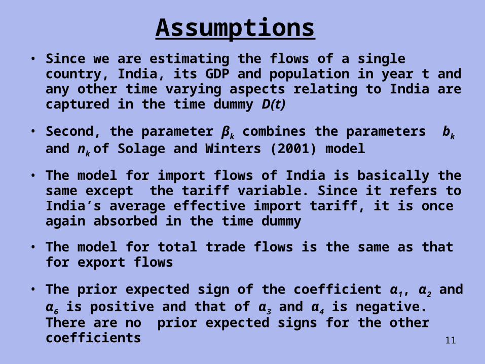
Assumptions • Since we are estimating the flows of a single country, India, its

GDP and population in year t and any other time varying aspects relating to India are captured in the time dummy D(t)

• Second, the parameter βk combines the parameters bk and nk of Solage and Winters (2001) model

• The model for import flows of India is basically the same except the tariff variable. Since it refers to India’s average effective import tariff, it is once again absorbed in the time dummy

• The model for total trade flows is the same as that for export flows

• The prior expected sign of the coefficient α1, α2 and α6 is positive and that of α3 and α4 is negative. There are no prior expected signs for the other coefficients

12

Data Sources • The data used are annual bilateral trade flows of India for the period 1981-

2006 for 189 countries.

• Data on GDP, GDP per capita, population, total exports, total imports and exchange rates are obtained from the World Development Indicators (WDI) database of the World Bank, and the International Financial Statistics (IFS).

• Data on India’s exports of goods and services, India’s imports of goods and services from and India's total trade of goods and services (exports plus imports) with the world are obtained from the Direction of Trade Statistics Yearbook (various issues) of IMF

• GDP, GDP per capita are in constant 1995 US dollars. GDP, total exports, total imports, India's exports, India’s imports and India’s total trade are measured in million US dollars.

• Population of the countries are in million.

• Data on the exchange rates are units in national currency per US dollar.

13

Data MFN Tariff: 

• The MFN tariff is taken from UNCTAD Handbook of Statistics database

• Here the MFN is taken as a simple average of tariffs for "Manufactured Goods, Ores and Metals" 

• The actual classification as per SITC code is

• Manufactured goods: 5+6+7+8-68

• Ores and Metals: 27+28+68

• 5.0 Chemicals and related products

• 6.0 Manufactured goods classified chiefly by material

• 7.0 Machinery and transport equipment

• 8.0 Miscellaneous manufactured articles

• 27. Crude fertilizers and crude materials (Excluding Coal)

• 28. Multi ferrous ores and metal scrap

14

Results

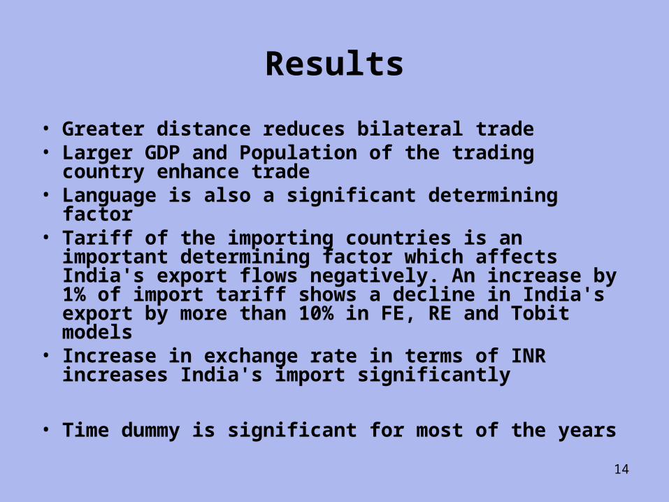
• Greater distance reduces bilateral trade• Larger GDP and Population of the trading country

enhance trade• Language is also a significant determining factor• Tariff of the importing countries is an important

determining factor which affects India's export flows negatively. An increase by 1% of import tariff shows a decline in India's export by more than 10% in FE, RE and Tobit models

• Increase in exchange rate in terms of INR increases India's import significantly

• Time dummy is significant for most of the years

15

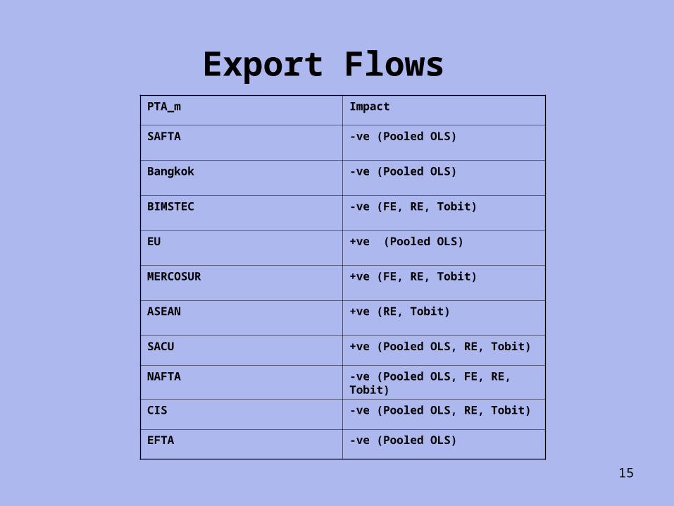
Export FlowsPTA_m Impact

SAFTA -ve (Pooled OLS)

Bangkok -ve (Pooled OLS)

BIMSTEC -ve (FE, RE, Tobit)

EU +ve (Pooled OLS)

MERCOSUR +ve (FE, RE, Tobit)

ASEAN +ve (RE, Tobit)

SACU +ve (Pooled OLS, RE, Tobit)

NAFTA -ve (Pooled OLS, FE, RE, Tobit)

CIS -ve (Pooled OLS, RE, Tobit)

EFTA -ve (Pooled OLS)

16

Import FlowsPTA_x Impact

SAFTA -ve (FE, RE)

Bangkok -ve (Pooled OLS)

BIMSTEC +ve (Pooled OLS, FE, RE)

EU +ve (Pooled OLS)

MERCOSUR +ve (FE, RE)

CIS +ve (FE, RE)

GCC +ve (Pooled OLS)

NAFTA -ve (FE, RE)

ASEAN -ve (FE, RE)

SACU -ve (Pooled OLS, Tobit)

17

Trade FlowsPTA_x +PTA_m Impact

SAFTA -ve (Pooled OLS)

Bangkok -ve (Pooled OLS)

BIMSTEC +ve (Pooled OLS, RE, Tobit)

EU +ve (Pooled OLS, RE, Tobit)

MERCOSUR +ve (FE)

GCC +ve (Tobit)

ASEAN -ve ( Pooled OLS, Tobit)

NAFTA -ve (Pooled OLS, Tobit)

18

Determinants of Export Decision of Firms

• Bernard, Jensen, Redding and Schott (2007)

• One robust finding of this literature, based on wide range of countries and industries, is that exporting firms tend to be larger, more productive, more intensive in skill and capital and pay higher wages than non-exporting firms

19

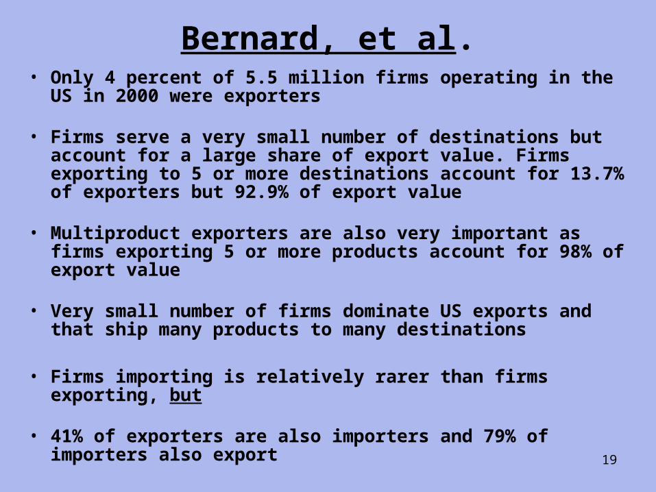
Bernard, et al.• Only 4 percent of 5.5 million firms operating in the US in 2000

were exporters

• Firms serve a very small number of destinations but account for a large share of export value. Firms exporting to 5 or more destinations account for 13.7% of exporters but 92.9% of export value

• Multiproduct exporters are also very important as firms exporting 5 or more products account for 98% of export value

• Very small number of firms dominate US exports and that ship many products to many destinations

• Firms importing is relatively rarer than firms exporting, but

• 41% of exporters are also importers and 79% of importers also export

20

• Roberts and Tybout (1997) and Aitken, Hanson and Harrision (1997) examine factors influencing the export decision

• They found that sunk costs are important influences on the export performance of firms

• They also provide evidence supporting that firm characteristics are important and find that firm size, firm age and the structure of ownership are positively related to the propensity to export

• Melitz (2003) provides a mechanism for today’s export decision by the firm to influence its future decision to export by incorporating entry costs in a dynamic framework

21

Export Determinants of Indian Manufacturing Firms

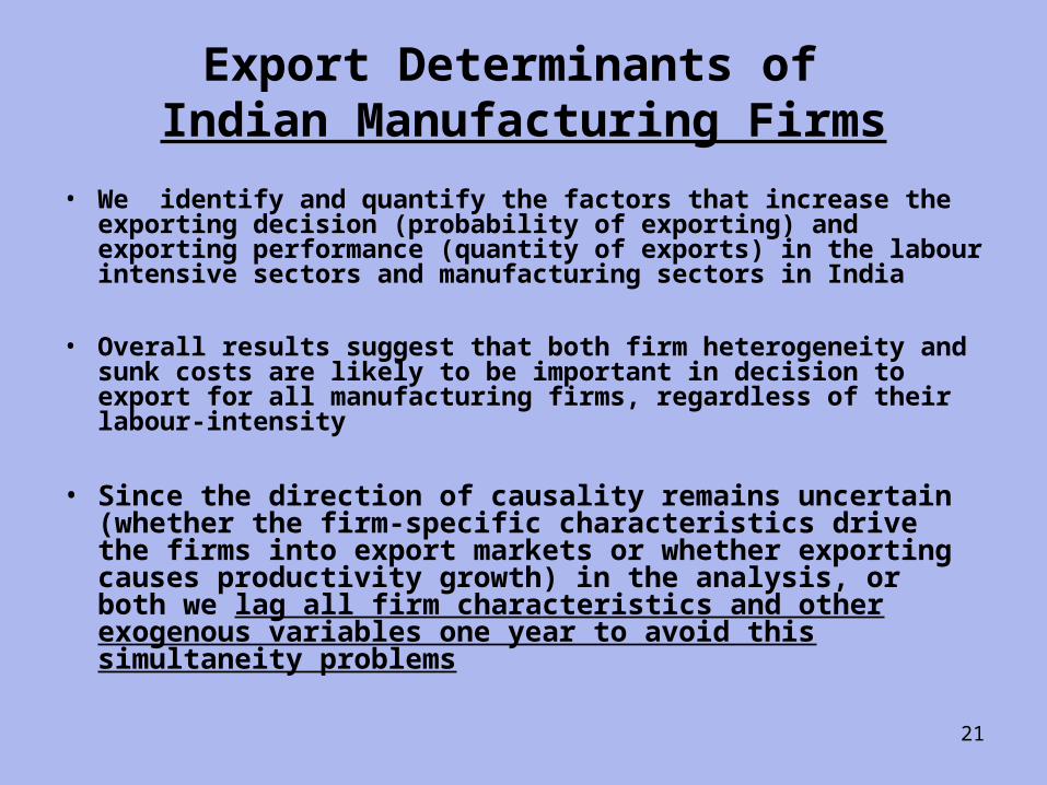
• We identify and quantify the factors that increase the exporting decision (probability of exporting) and exporting performance (quantity of exports) in the labour intensive sectors and manufacturing sectors in India

• Overall results suggest that both firm heterogeneity and sunk costs are likely to be important in decision to export for all manufacturing firms, regardless of their labour-intensity

• Since the direction of causality remains uncertain (whether the firm-specific characteristics drive the firms into export markets or whether exporting causes productivity growth) in the analysis, or both we lag all firm characteristics and other exogenous variables one year to avoid this simultaneity problems

22

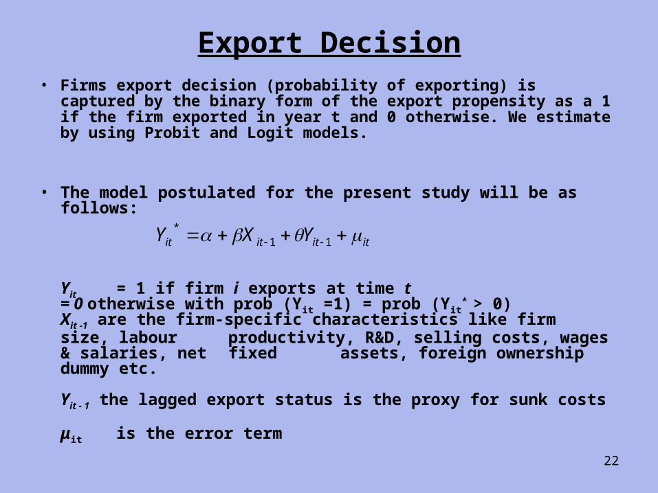
Export Decision• Firms export decision (probability of exporting) is captured by the

binary form of the export propensity as a 1 if the firm exported in year t and 0 otherwise. We estimate by using Probit and Logit models.

• The model postulated for the present study will be as follows:

Yit = 1 if firm i exports at time t= 0 otherwise with prob (Yit =1) = prob (Yit

* > 0)Xit -1 are the firm-specific characteristics like firm size, labour productivity, R&D, selling costs, wages & salaries, net fixed assets, foreign ownership dummy etc.

Yit - 1 the lagged export status is the proxy for sunk costs

μit is the error term

itititit YXY 11*

23

Export Performance • Firms export performance (quantity of exports) is captured by the binary

form of the export propensity as a percentage of total sales if the firm exported in year t and 0 otherwise. We estimate by using Tobit model with a binary variable

The structure of the Tobit model panel data with random effects would be:

• Yit = Yit* if Yit * > 0 (the value exported as a percentage of sale by firm i in

year t) = 0 otherwise

where, Yit is a linear function of (Xit - 1), the firm-specific characteristics like firm size, labour productivity, R&D, selling costs, value added per worker etc.

• Yit - 1 is the lagged export

itititit YXY 11*

24

Variables

Sunk Costs• Sunk costs are costs associated with entering foreign markets and any

fixed entry costs that may have the character of being sunk (i.e. once incurred can not be recovered) in nature

• Sunk cost could induce persistent in the time pattern of export decisions

• In the present study sunk cost is inferred from the sequence of exporting and non-exporting years, rather than frequent and apparently random switching between the two

• Also lagged export status has been taken as the proxy for sunk costs

25

Entry & Exit

• Distribution of firms in labour intensive activities across all the 103 possible sequences of exporting and non-exporting for the seven years from 2000-2006 show that -

– 33 % exports in all seven years and an equally large fraction, 30 %, never export

– In the all manufacturing firms – fraction of firms who never exported doubled to 41% as compared to 21% who exported throughout the period

26

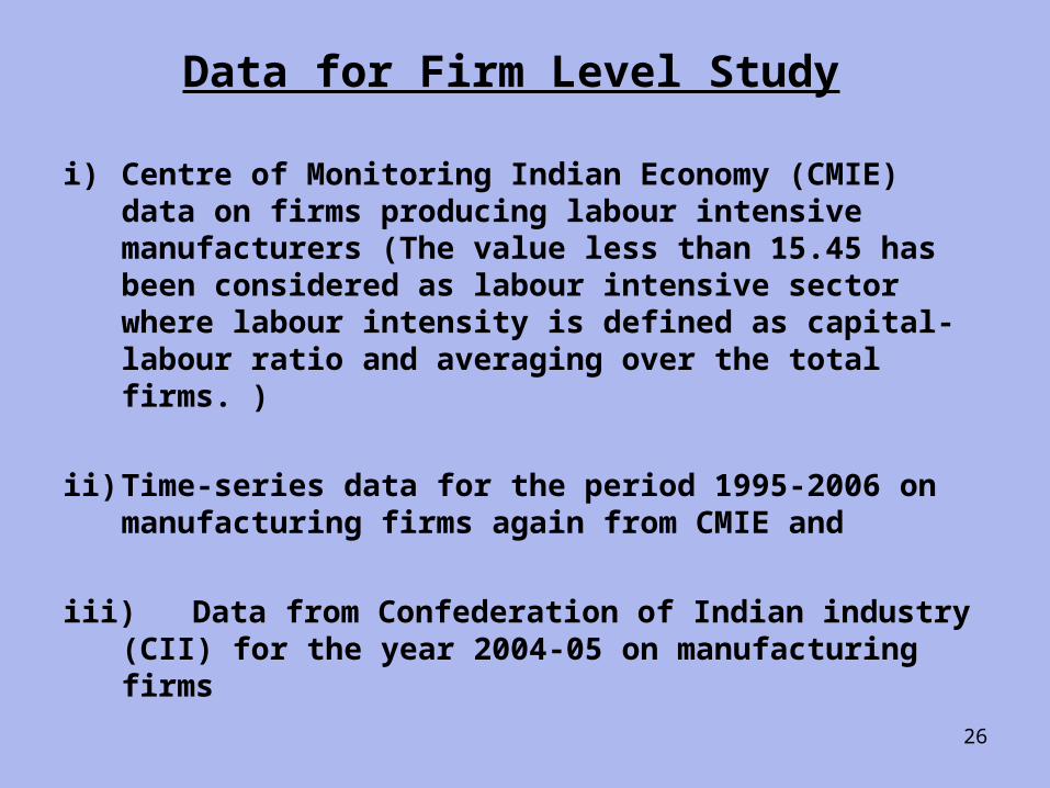
Data for Firm Level Study

i) Centre of Monitoring Indian Economy (CMIE) data on firms producing labour intensive manufacturers (The value less than 15.45 has been considered as labour intensive sector where labour intensity is defined as capital-labour ratio and averaging over the total firms. )

ii) Time-series data for the period 1995-2006 on manufacturing firms again from CMIE and

iii) Data from Confederation of Indian industry (CII) for the year 2004-05 on manufacturing firms

27

Foreign Ownership

The percentage of firms with the majority of foreign capital participation in the group of exporters is 30.85 whereas in the group of non-exporters the rate of foreign participation is 16.22 in the data from CII

Thus the degree of foreign owned companies in the population of exporters is high and is expected to be positively related to exporting

Foreign ownership is a dummy variable which is equal to 1 if firms either have a Joint Ventures/Collaboration/foreign parent and 0 otherwise

28

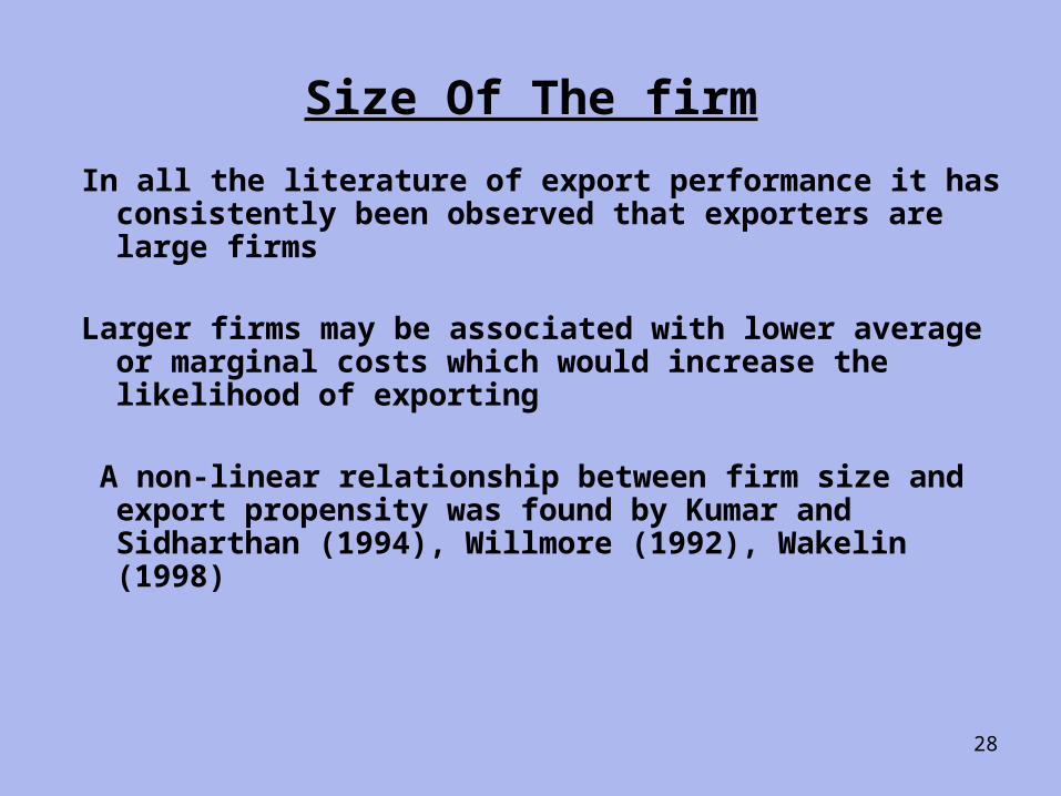
Size Of The firm

In all the literature of export performance it has consistently been observed that exporters are large firms

Larger firms may be associated with lower average or marginal costs which would increase the likelihood of exporting

A non-linear relationship between firm size and export propensity was found by Kumar and Sidharthan (1994), Willmore (1992), Wakelin (1998)

29

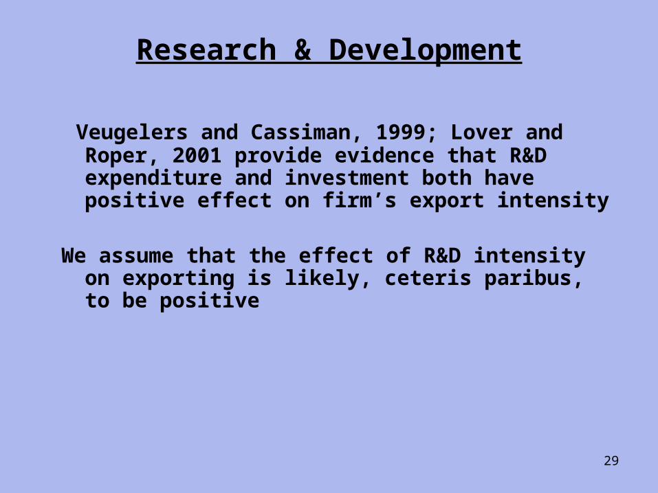
Research & Development

Veugelers and Cassiman, 1999; Lover and Roper, 2001 provide evidence that R&D expenditure and investment both have positive effect on firm’s export intensity

We assume that the effect of R&D intensity on exporting is likely, ceteris paribus, to be positive

30

Wages

The lower is the real wage, the greater is the firm’s competitive advantage which is expected to result in higher volume of exports

This is an implication of comparative advantage from the relative abundance of labour endowment which provides cost competitiveness for firms at micro-level

31

Labour Productivity

It is not just the low labour cost that leads to comparative cost advantage but low wage in relation to productivity of that labour which determines the export performance

32

Selling Costs

• Firms have to develop distributional network especially if they have to operate in the international market

• Hence marketing and sales expenses are expected to lead to higher probability of exporting

33

Energy Intensity

• Energy-intensity, measured in terms of power and fuel expenditure as a proportion of sale, is another important factor that may influence export performance

• A positive relationship between export and energy-intensity is expected since an industry with higher energy intensity could be more efficient and competitive

• On the other hand as a cost it would adversely affect export sales

34

Capital Intensity

• Capital intensity, measured in terms of net fixed asset as a proportion of sale is total fixed assets net of accumulated depreciation

• Net fixed assets include capital work-in-progress and revalued assets

35

Profit Intensity

• Only those who can produce above the export productivity cut-off can export in equilibrium (Melitz, 2003)

• Hence we hypothesize that firms with higher profit per unit of sales are more probable of exporting and competiting in world market

36

Import Intensity

• Higher import intensity are more likely to export

• Higher import intensity reflects greater ability to import by exporting firms

37

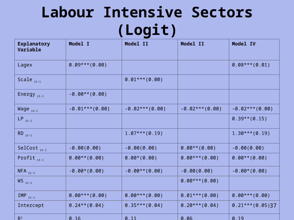
Labour Intensive Sectors (Logit)Explanatory Variable

Model I Model II Model II Model IV

Lagex 0.09***(0.00) 0.08***(0.01)

Scale it-1 0.01***(0.00)

Energy it-1 -0.00**(0.00)

Wage it-1 -0.01***(0.00) -0.02***(0.00) -0.02***(0.00) -0.02***(0.00)

LP it-1 0.39**(0.15)

RD it-1 1.07***(0.19) 1.30***(0.19)

SelCost it-1 -0.00(0.00) -0.00(0.00) 0.00**(0.00) -0.00(0.00)

Profit it-1 0.00**(0.00) 0.00*(0.00) 0.00***(0.00) 0.00**(0.00)

NFA it-1 -0.00*(0.00) -0.00**(0.00) -0.00(0.00) -0.00*(0.00)

WS it-1 0.00***(0.00)

IMP it-1 0.00***(0.00) 0.00***(0.00) 0.01***(0.00) 0.00***(0.00)

Intercept 0.24**(0.04) 0.35***(0.04) 0.20***(0.04) 0.21***(0.05)

R2 0.16 0.11 0.06 0.19

38

Labour Intensive Sectors (Probit)Explanatory Variable

Model I Model II Model II Model IV

Lagex 0.02***(0.00) 0.03*** (0.00)

Scale it-1 0.00*** (0.00)

Energy it-1 -0.00 (0.00)

Wage it-1 -0.01*** (0.00) -0.01*** (0.00) -0.01*** (0.00) -0.01*** (0.00)

LP it-1 0.18** (0.07)

RD it-1 0.55*** (0.08) 0.57*** (0.08)

SelCost it-1 -0.07 (0.01) 0.14** (0.00) -0.08 (0.01) -0.12 (0.00)

Profit it-1 0.00** (0.00) 0.00*** (0.00) 0.00** (0.00) 0.00*** (0.00)

NFA it-1 -0.00** (0.00) -0.00 (0.00) -0.00** (0.00) -0.00** (0.00)

Wshare1 it-1 0.00*** (0.00)

IMP it-1 0.01*** (0.00) 0.00*** (0.00)

Intercept 0.24*** (0.02) 0.54*** (0.02) 0.25*** (0.02) 0.30*** (0.02)

R2 0.16 0.05 0.15 0.09

39

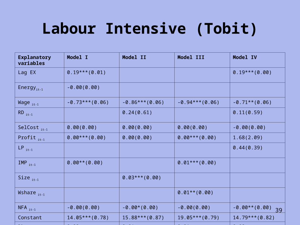
Labour Intensive (Tobit)

Explanatoryvariables

Model I Model II Model III Model IV

Lag EX 0.19***(0.01) 0.19***(0.00)

Energyit-1 -0.00(0.00)

Wage it-1 -0.73***(0.06) -0.86***(0.06) -0.94***(0.06) -0.71**(0.06)

RD it-1 0.24(0.61) 0.11(0.59)

SelCost it-1 0.00(0.00) 0.00(0.00) 0.00(0.00) -0.00(0.00)

Profit it-1 0.00***(0.00) 0.00(0.00) 0.00***(0.00) 1.68(2.09)

LP it-1 0.44(0.39)

IMP it-1 0.00**(0.00) 0.01***(0.00)

Size it-1 0.03***(0.00)

Wshare it-1 0.01**(0.00)

NFA it-1 -0.00(0.00) -0.00*(0.00) -0.00(0.00) -0.00**(0.00)

Constant 14.05***(0.78) 15.88***(0.87) 19.05***(0.79) 14.79***(0.82)

R2 0.02 0.01 0.01 0.02

40

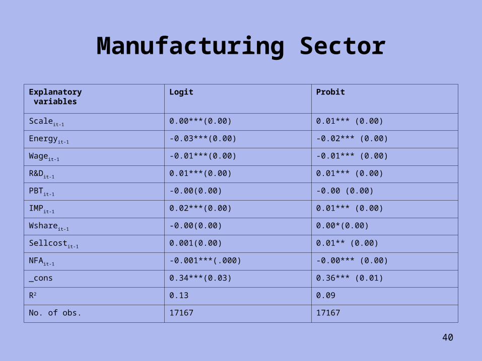
Manufacturing Sector

Explanatory variables

Logit Probit

Scaleit-1 0.00***(0.00) 0.01*** (0.00)

Energyit-1 -0.03***(0.00) -0.02*** (0.00)

Wageit-1 -0.01***(0.00) -0.01*** (0.00)

R&Dit-1 0.01***(0.00) 0.01*** (0.00)

PBTit-1 -0.00(0.00) -0.00 (0.00)

IMPit-1 0.02***(0.00) 0.01*** (0.00)

Wshareit-1 -0.00(0.00) 0.00*(0.00)

Sellcostit-1 0.001(0.00) 0.01** (0.00)

NFAit-1 -0.001***(.000) -0.00*** (0.00)

_cons 0.34***(0.03) 0.36*** (0.01)

R2 0.13 0.09

No. of obs. 17167 17167

41

Manufacturing Sector (Tobit)

Explanatory variables Model I Model II

LagEx 0.02***(0.00)

Scaleit-1 0.00 (0.00)

Energyit-1 -0.01***(0.00) -0.01*** (0.00)

Wageit-1 -0.01***(0.00) -0.00*** (0.00)

R&Dit-1 0.01(0.00) 0.01 (0.00)

PBTit-1 -0.00(0.00) -0.00 (0.00)

IMPit-1 0.02***(0.00) 0.01*** (0.00)

Wshareit-1 0.03***(0.00) 0.02***(0.00)

Sellcostit-1 0.001(0.00) -0.01 (0.00)

NFAit-1 -0.001(.000) -0.00 (0.00)

_cons 4.73***(0.05) 4.44*** (0.05)

No. of obs. 17167 17167

42

CII (Manufacturing)Variables Tobit Model

Scale 1.80***(0.94)

Own 2.39***(0.85)

Sale/no of emp -0.23(2.88)

CP -2.30e-07 (4.74e-06)

Const 4.82***(0.48)

Note: standard error in parenthesisDependent variable = 0 for the non-exporting yearsExport as percentage of total sales if they did export in period t.Scale is a dummy that takes value = 1 if it is a large firm and = 0 otherwiseOwn is a dummy that takes value = 1 if firm either have a JV/Collaboration /foreign parent and 0 otherwiseCP (capital productivity) = total turnover/ investment

43

A Hazard Model

• We have tried to estimate the probability of a firm exporting in any year based on its characteristics

• Data on manufacturing firms in India during 1995-2006 are used for this purpose

44

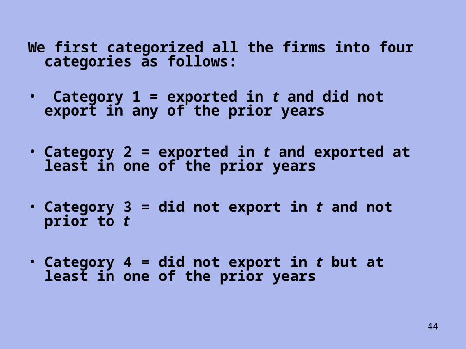
We first categorized all the firms into four categories as follows:

• Category 1 = exported in t and did not export in any of the prior years

• Category 2 = exported in t and exported at least in one of the prior years

• Category 3 = did not export in t and not prior to t

• Category 4 = did not export in t but at least in one of the prior years

45

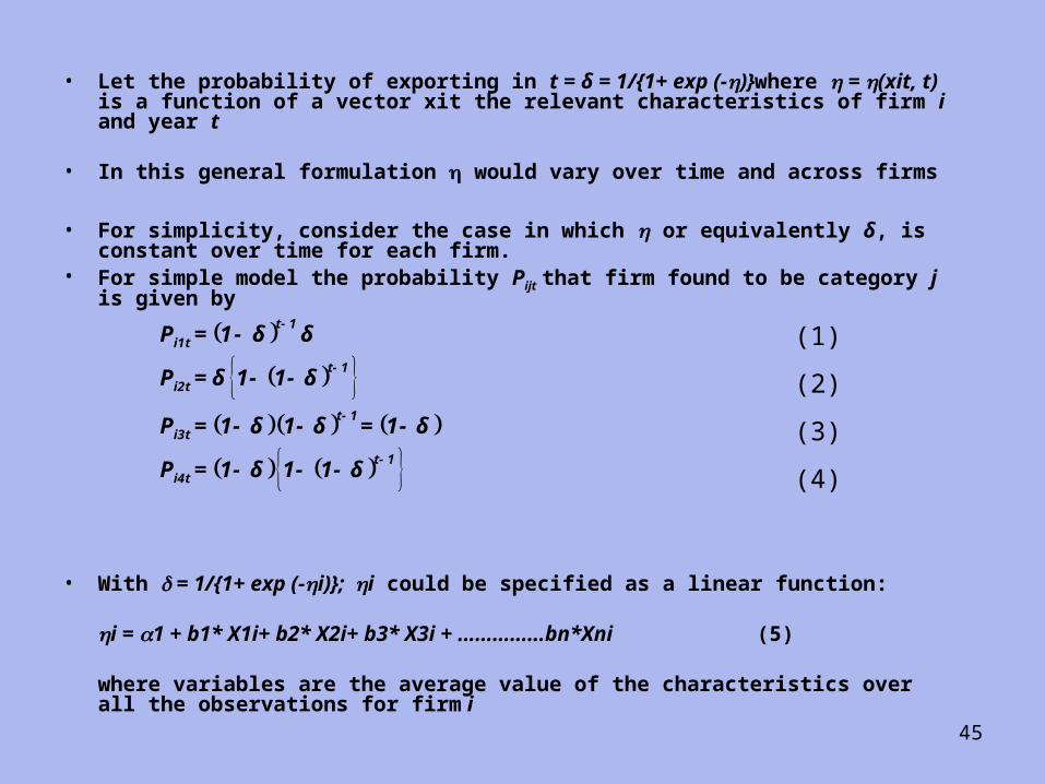
• Let the probability of exporting in t = δ = 1/{1+ exp (-)}where = (xit, t) is a function of a vector xit the relevant characteristics of firm i and year t

• In this general formulation would vary over time and across firms

• For simplicity, consider the case in which or equivalently δ, is constant over time for each firm.

• For simple model the probability Pijt that firm found to be category j is given by

• With = 1/{1+ exp (-i)}; i could be specified as a linear function:

i = 1 + b1* X1i+ b2* X2i+ b3* X3i + ……………bn*Xni (5)

where variables are the average value of the characteristics over all the observations for firm i

t- 1

i1t

t- 1

i2t

t- 1

i3t

t- 1

i4t

P = 1- δ δ

P =δ 1- 1- δ

P = 1- δ 1- δ = 1- δ

P = 1- δ 1- 1- δ

(1)

(2)

(3)

(4)

46

• The model which we estimated is a simpler multinomial Logit model for Pijt.

• In other words, given that by definition treating the third category as the reference category we postulate that log odds of category j relative to 3 as

• for j = 1, 2 and 4

{Xkit} are characteristics of firms i in year t

4

ijtj=1

P =1

+ n

ijt i3t j jk kitk=1

Log (P /P ) = α b X

47

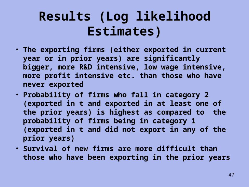
Results (Log likelihood Estimates)

• The exporting firms (either exported in current year or in prior years) are significantly bigger, more R&D intensive, low wage intensive, more profit intensive etc. than those who have never exported

• Probability of firms who fall in category 2 (exported in t and exported in at least one of the prior years) is highest as compared to the probability of firms being in category 1 (exported in t and did not export in any of the prior years)

• Survival of new firms are more difficult than those who have been exporting in the prior years

48

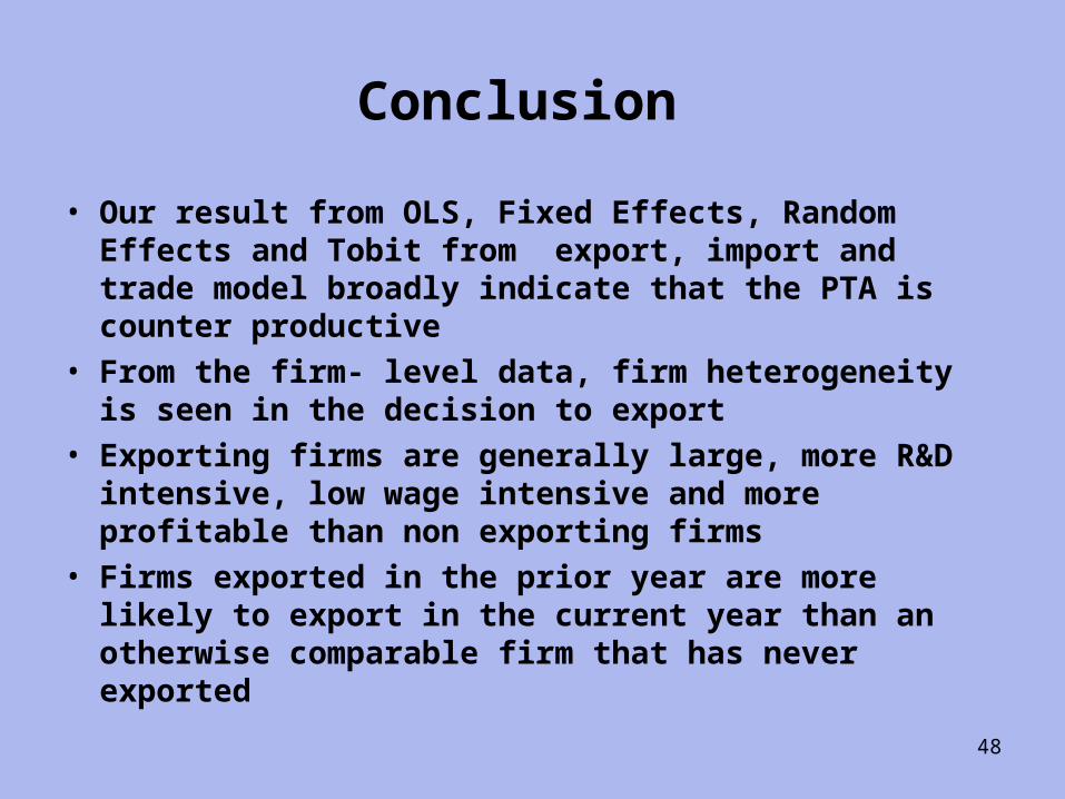
Conclusion

• Our result from OLS, Fixed Effects, Random Effects and Tobit from export, import and trade model broadly indicate that the PTA is counter productive

• From the firm- level data, firm heterogeneity is seen in the decision to export

• Exporting firms are generally large, more R&D intensive, low wage intensive and more profitable than non exporting firms

• Firms exported in the prior year are more likely to export in the current year than an otherwise comparable firm that has never exported

49

THANK YOU