TM1 Demand Estimates 140806 - Sacramento County, California

1772 Picasso Ave, Suite A 1 phone 530.757.6107 Davis, CA 95618-0550 www.davidsengineering.com

Specialists in Agricultural Water Management Serving Stewards of Water in the West since 1993

TechnicalMemorandumTo: RMC Water and Environment

From: Davids Engineering

Date: May 7, 2014

Subject: Sacramento Central Groundwater Authority 2011‐2012 Agricultural Demand and

Groundwater Pumping Estimates

OverviewThis technical memorandum describes an analysis of agricultural water demands for irrigation and

corresponding groundwater use for 2011 and 2012 within the boundaries of the Sacramento Central

Groundwater Authority (SCGA), hereinafter referred to as the Study Area. The analysis was performed

for field polygons potentially under agricultural production based on land use information compiled by

the Sacramento Area Council of Governments (SACOG, Bell 2013). The Study Area and field polygons

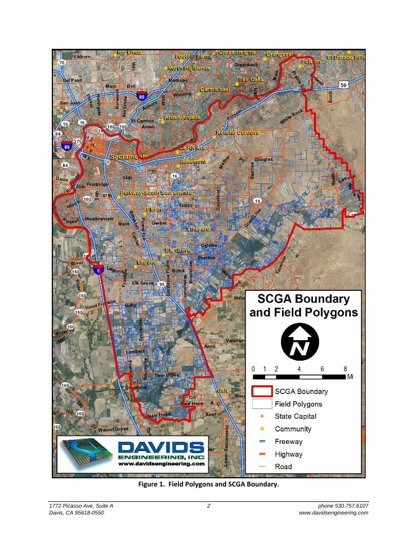
are shown in Figure 1. The Study Area is generally bounded by the American River on the north,

Interstate 5 on the west, New Hope Road and Dillard Road on the south, and Prairie City and Scott Road

on the east. Land uses and types outside of the Sacramento urban area include native and riparian

vegetation, agriculture, and rural residential development. Agriculture is most dense along the

Cosumnes River and is almost wholly dependent on groundwater for irrigation.

The analysis of irrigation demands was performed for agricultural and rural residential lands in the area.

Existing land use data developed by SACOG for 2008 were updated to reflect 2011 and 2012 cropping

based on information from the Cropland Data Layer (CDL) developed by the National Agricultural

Statistics Service (NASS)1. Then, evapotranspiration (ET) was estimated using a crop coefficient‐

reference evapotranspiration calculation approach as described by Allen et al. (1998). Crop coefficients

were developed based on available Surface Energy Balance Algorithm for Land (SEBAL, Bastiaanssen et

al., 2005) data describing actual ET for the 2009 growing season covering the study area.

Following the estimation of total actual ET, the Integrated Water Flow Model (IWFM) Demand

Calculator (IDC) version 4.0.286 (DWR 2013) was configured and applied to perform daily root‐zone‐

water‐balance calculations for 2011 and 2012 and to estimate of the amount of ET derived from applied

irrigation water (ETaw) and from precipitation (ETpr) for individual crop‐soil groups. IDC was then

configured and run to estimate applied water (irrigation) demands.

1 Available at http://nassgeodata.gmu.edu/CropScape/. Accessed 2/24/2014.


Figure 1. Field Polygons and SCGA Boundary.


Developmentof2011and2012AgriculturalLandUse

This section describes the development of agricultural land use estimates for SCGA for 2011 and 2012.

DevelopmentofLandUseClassesGeneral land use classes with similar ET demands and irrigation practices were developed for the Study

Area to provide consistency between the land use classes in SACOG 2008 and those in the CDL. Four

agricultural land use classes were developed for agricultural land (Fallow, Field and Truck, Pasture and

Hay, and Vineyards and Orchards), two for native vegetation (Native and Riparian/Wetlands), and one

for rural residential. These classes are summarized in Table 1, along with corresponding land use

classes in 2008, the number of field polygons, and the acreage for each class.

Table 1. Land Use Classes for Ag Water Demand Update for SCGA, 2011‐2012.

SCGA Land Use SACOG Land Uses Number of Polygons Acres

Fallow Fallow, Other, Other Agriculture 146 3,728

Field and Truck Beans, dry; Corn; Field Crops; Large Scale Local Vegetables; Rice; Safflower; Tomatoes, processing

311 10,309

Pasture and Hay

Alfalfa; Grass Hay; Hay, all; Pasture; Pasture/Natural Vegetation; Sudan Grass; Wheat

1,220 24,406

Vineyards and Orchards

Citrus, Grapes, Grapes/Vineyards, Fruits & Nuts unspecified, Nursery, Other, Walnuts

209 8,292

Native

Fallow; Natural Vegetation; Natural Vegetation/Wetlands; Other; Other Agriculture; Pasture/Natural Vegetation; Rural Residential/Developed

637 46,882

Riparian/ Wetlands

Natural Vegetation; Natural Vegetation/Wetlands; Pasture/Natural Vegetation

304 8,444

Rural Residential

Natural Vegetation/Wetlands; Other; Pasture/Natural Vegetation; Rural Residential/Developed

2,238 11,943

The land use from the 2008 SACOG data was reclassified and updated based on more recent land use

data and based on visual inspection of available aerial and satellite imagery. As a result, some of the

SACOG 2008 land use classes are listed more than once corresponding to different SCGA Land Uses. For

example, the SACOG land use “Natural Vegetation” (Column 2 in Table 1) is listed under the “Native”, as

well as “Native and Riparian/Wetlands SCGA” land use classes (Column 1 in Table 1). The reason is that

fine‐scale riparian mapping data (CDFW 2013) is available to differentiate “Native” and

“Riparian/Wetlands”, both previously designated as “Natural Vegetation”. The process is described in

the following section.


Similarly, the CDL data were assigned (or reclassified) to the seven SCGA land use types developed in the

SACOG 2008 land use reclassifying process. The cross‐references developed to reclassify the CDL data

are provided in Table 2. Although many of the CDL land uses were not found in the SCGA area, all CDL

land use classes were assigned to a general SCGA land use type to facilitate future updates.


Table 2. SCGA Land Use Classes and Corresponding CDL Land Use Classes.

SCGA Land Use

CDL

Code CDL Land Use SCGA Land Use

CDL

Code CDL Land Use SCGA Land Use

CDL

Code CDL Land Use

Fallow 61 Fallow/Idle Cropland Field and Truck 226 Dbl Crop Oats/Corn Pasture and Hay 59 Sod/Grass Seed

Field and Truck 1 Corn Field and Truck 227 Lettuce Pasture and Hay 60 Switchgrass

Field and Truck 2 Cotton Field and Truck 229 Pumpkins Pasture and Hay 176 Grassland/Pasture

Field and Truck 3 Rice Field and Truck 230 Dbl Crop Lettuce/Durum Wht Pasture and Hay 205 Triticale

Field and Truck 4 Sorghum Field and Truck 231 Dbl Crop Lettuce/Cantaloupe Pasture and Hay 224 Vetch

Field and Truck 5 Soybeans Field and Truck 232 Dbl Crop Lettuce/Cotton Riparian/Wetlands 87 Wetlands

Field and Truck 6 Sunflower Field and Truck 233 Dbl Crop Lettuce/Barley Riparian/Wetlands 190 Woody Wetlands

Field and Truck 10 Peanuts Field and Truck 234 Dbl Crop Durum Wht/Sorghum Riparian/Wetlands 195 Herbaceous Wetlands

Field and Truck 11 Tobacco Field and Truck 235 Dbl Crop Barley/Sorghum Riparian/Wetlands 83 Water

Field and Truck 12 Sweet Corn Field and Truck 236 Dbl Crop WinWht/Sorghum Riparian/Wetlands 92 Aquaculture

Field and Truck 13 Popcorn or Ornamental Corn Field and Truck 237 Dbl Crop Barley/Corn Riparian/Wetlands 111 Open Water

Field and Truck 14 Mint Field and Truck 238 Dbl Crop WinWht/Cotton Rural Residential 82 Developed

Field and Truck 23 Spring Wheat Field and Truck 239 Dbl Crop Soybeans/Cotton Rural Residential 121 Developed/Open Space

Field and Truck 26 Dbl Crop WinWht/Soybeans Field and Truck 240 Dbl Crop Soybeans/Oats Rural Residential 122 Developed/Low Intensity

Field and Truck 31 Canola Field and Truck 241 Dbl Crop Corn/Soybeans Rural Residential 123 Developed/Med Intensity

Field and Truck 33 Safflower Field and Truck 243 Cabbage Rural Residential 124 Developed/High Intensity

Field and Truck 34 Rape Seed Field and Truck 244 Cauliflower Vineyards and Orchards 55 Caneberries

Field and Truck 35 Mustard Field and Truck 245 Celery Vineyards and Orchards 66 Cherries

Field and Truck 41 Sugarbeets Field and Truck 246 Radishes Vineyards and Orchards 67 Peaches

Field and Truck 42 Dry Beans Field and Truck 247 Turnips Vineyards and Orchards 68 Apples

Field and Truck 43 Potatoes Field and Truck 248 Eggplants Vineyards and Orchards 69 Grapes

Field and Truck 45 Sugarcane Field and Truck 249 Gourds Vineyards and Orchards 70 Christmas Trees

Field and Truck 46 Sweet Potatoes Field and Truck 254 Dbl Crop Barley/Soybeans Vineyards and Orchards 71 Other Tree Crops

Field and Truck 47 Misc Vegs & Fruits Native 63 Forest Vineyards and Orchards 72 Citrus

Field and Truck 48 Watermelons Native 64 Shrubland Vineyards and Orchards 74 Pecans

Field and Truck 49 Onions Native 65 Barren Vineyards and Orchards 75 Almonds

Field and Truck 50 Cucumbers Native 131 Barren Vineyards and Orchards 76 Walnuts

Field and Truck 51 Chick Peas Native 143 Mixed Forest Vineyards and Orchards 77 Pears

Field and Truck 52 Lentils Native 152 Shrubland Vineyards and Orchards 141 Deciduous Forest

Field and Truck 53 Peas Pasture and Hay 21 Barley Vineyards and Orchards 142 Evergreen Forest

Field and Truck 54 Tomatoes Pasture and Hay 22 Durum Wheat Vineyards and Orchards 204 Pistachios

Field and Truck 56 Hops Pasture and Hay 24 Winter Wheat Vineyards and Orchards 210 Prunes

Field and Truck 57 Herbs Pasture and Hay 25 Other Small Grains Vineyards and Orchards 211 Olives

Field and Truck 206 Carrots Pasture and Hay 27 Rye Vineyards and Orchards 212 Oranges

Field and Truck 207 Asparagus Pasture and Hay 28 Oats Vineyards and Orchards 217 Pomegranates

Field and Truck 208 Garlic Pasture and Hay 29 Millet Vineyards and Orchards 218 Nectarines

Field and Truck 209 Cantaloupes Pasture and Hay 30 Speltz Vineyards and Orchards 220 Plums

Field and Truck 213 Honeydew Melons Pasture and Hay 32 Flaxseed Vineyards and Orchards 223 Apricots

Field and Truck 214 Broccoli Pasture and Hay 36 Alfalfa Vineyards and Orchards 242 Blueberries

Field and Truck 216 Peppers Pasture and Hay 37 Other Hay/Non Alfalfa Vineyards and Orchards 250 Cranberries

Field and Truck 219 Greens Pasture and Hay 38 Camelina Unassigned 81 Clouds/No Data

Field and Truck 221 Strawberries Pasture and Hay 39 Buckwheat Unassigned 88 Nonag/Undefined

Field and Truck 222 Squash Pasture and Hay 44 Other Crops Unassigned 112 Perennial Ice/Snow

Field and Truck 225 Dbl Crop WinWht/Corn Pasture and Hay 58 Clover/Wildflowers


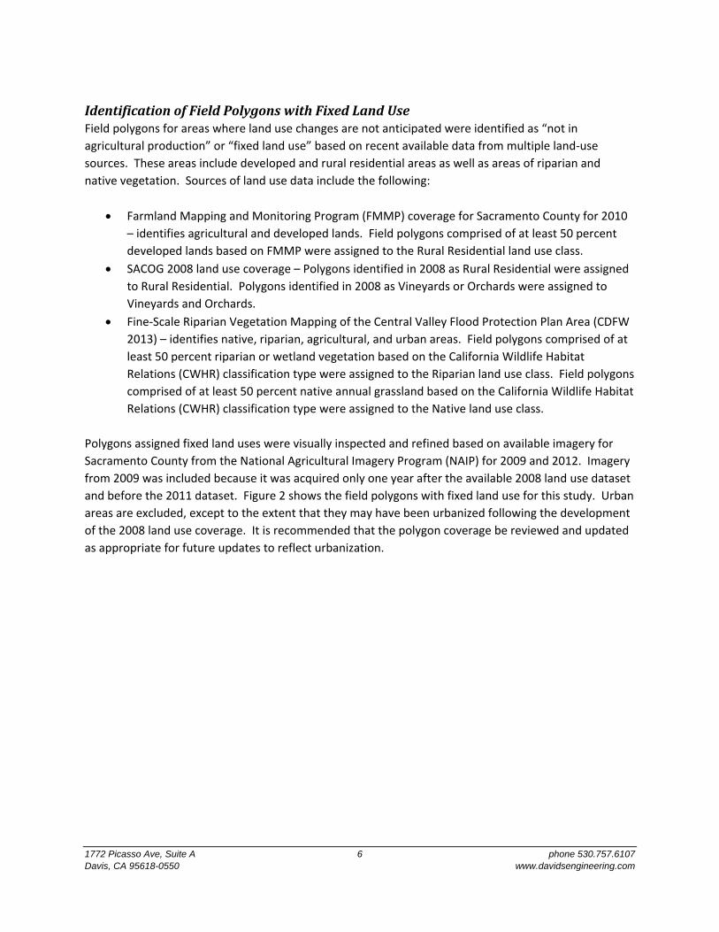
IdentificationofFieldPolygonswithFixedLandUseField polygons for areas where land use changes are not anticipated were identified as “not in

agricultural production” or “fixed land use” based on recent available data from multiple land‐use

sources. These areas include developed and rural residential areas as well as areas of riparian and

native vegetation. Sources of land use data include the following:

Farmland Mapping and Monitoring Program (FMMP) coverage for Sacramento County for 2010

– identifies agricultural and developed lands. Field polygons comprised of at least 50 percent

developed lands based on FMMP were assigned to the Rural Residential land use class.

SACOG 2008 land use coverage – Polygons identified in 2008 as Rural Residential were assigned

to Rural Residential. Polygons identified in 2008 as Vineyards or Orchards were assigned to

Vineyards and Orchards.

Fine‐Scale Riparian Vegetation Mapping of the Central Valley Flood Protection Plan Area (CDFW

2013) – identifies native, riparian, agricultural, and urban areas. Field polygons comprised of at

least 50 percent riparian or wetland vegetation based on the California Wildlife Habitat

Relations (CWHR) classification type were assigned to the Riparian land use class. Field polygons

comprised of at least 50 percent native annual grassland based on the California Wildlife Habitat

Relations (CWHR) classification type were assigned to the Native land use class.

Polygons assigned fixed land uses were visually inspected and refined based on available imagery for

Sacramento County from the National Agricultural Imagery Program (NAIP) for 2009 and 2012. Imagery

from 2009 was included because it was acquired only one year after the available 2008 land use dataset

and before the 2011 dataset. Figure 2 shows the field polygons with fixed land use for this study. Urban

areas are excluded, except to the extent that they may have been urbanized following the development

of the 2008 land use coverage. It is recommended that the polygon coverage be reviewed and updated

as appropriate for future updates to reflect urbanization.


Figure 2. Field Polygons with Fixed Land Use.


Developmentof2011LandUse

This section describes land use assignment for 2011.

InitialLandUseAssignmentLand use for 2011 was estimated for each field polygon as follows:

1. Extract land use data by CDL pixel for each field polygon using ArcGIS Spatial Analyst.

2. Reclassify 2011 CDL to SCGA land use classes in MS Access.

3. Identify the SCGA land use class of majority for each polygon in MS Access.

4. For field polygons with fixed land use (3,095 field polygons comprising a total of 71,799 acres),

as described above, assign 2008 SACOG land use class.

5. For field polygons that are too small to contain CDL pixels (311 field polygons comprising a total

of 70 acres), assign 2008 SACOG land use class.

6. For remaining field polygons (1,659 field polygons comprising a total of 42,134 acres), assign the

SCGA land use class of majority (from step 3).

ValidationandRefinementofLandUseAssignmentFollowing the initial land use assignment, the following steps were completed to validate and refine the

results:

1. Select polygons without a fixed land use and without a crop covering at least 80% of each

polygon (based on 2011 CDL assigned land use). Visually inspect available aerial and satellite

imagery.

This resulted in identification of 18 fields making up 494 acres. Land use assignments for 2011

were modified from fallow to an agricultural land use for six fields based on review of available

Landsat (Clark et al. 2014) and NAIP imagery.

2. Select polygons with at least 80% of a particular crop in 2011 that differs from 2008 SCGA land

use class. Visually inspect available aerial and satellite imagery.

This resulted in identification of 324 fields comprising 11,514 acres. Of these, 188 fields 20 acres

or more comprising a total of 10,378 acres were visually inspected, and 2011 SCGA land use was

updated for 34 fields. Common changes include crop rotation from a pasture or hay crop to a

field or truck crop or idle or vice‐versa.

Developmentof2012LandUse

This section describes land use assignment for 2012.


InitialLandUseAssignmentLand use for 2012 was estimated for each field polygon as follows:

1. Extract land use data by CDL pixel for each field polygon using ArcGIS Spatial Analyst.

2. Reclassify 2012 CDL to SCGA land use classes in MS Access.

3. Identify the SCGA land use class of majority for each polygon in MS Access.

4. For field polygons with fixed land use (3,095 fields comprising a total of 71,799 acres), as

described above, assign 2008 SACOG land use class

5. For fields too small to contain CDL pixels (311 fields comprising a total of 70 acres), assign 2008

SACOG land use class.

6. For remaining fields (1,659 fields comprising a total of 42,134 acres), assign the 2012 SCGA land

use class of majority (from step 3).

ValidationandRefinementofLandUseAssignmentFollowing the initial land use assignment, the following steps were completed to validate and refine the

results:

1. Select polygons without a fixed land use and without a crop covering at least 80% of each

polygon (based on 2012 CDL assigned land use). Visually inspect available aerial and satellite

imagery.

This resulted in identification of 12 fields making up 219 acres. Land use assignments for 2012

were modified from fallow to an agricultural land use for three fields based on review of

available Landsat and NAIP imagery.

2. Select polygons with at least 80% of a particular crop in 2012 that differs from 2011 SCGA land

use class. Visually inspect available aerial and satellite imagery.

This resulted in identification of 188 fields comprising 5,222 acres. Of these, 97 fields 20 acres

or more comprising a total of 4,455 acres were visually inspected, and 2012 SCGA land use was

updated for 24 fields. Common changes include crop rotation from a pasture or hay crop to a

field or truck crop or idle or vice‐versa.

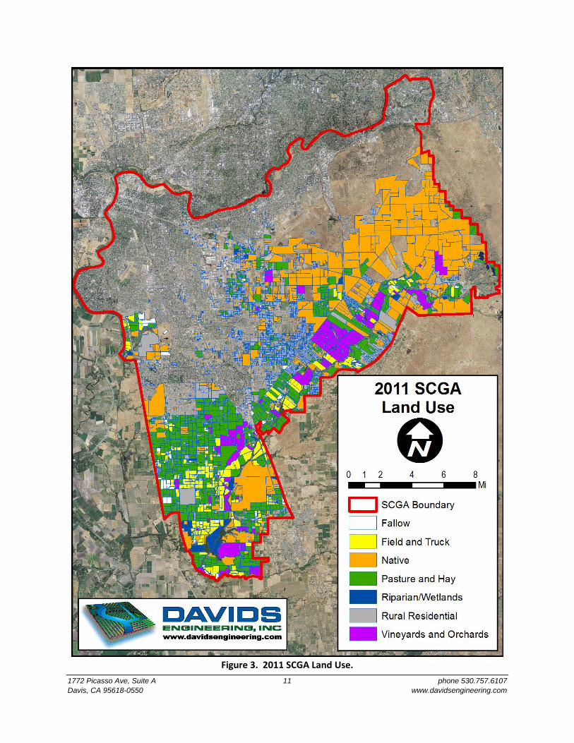
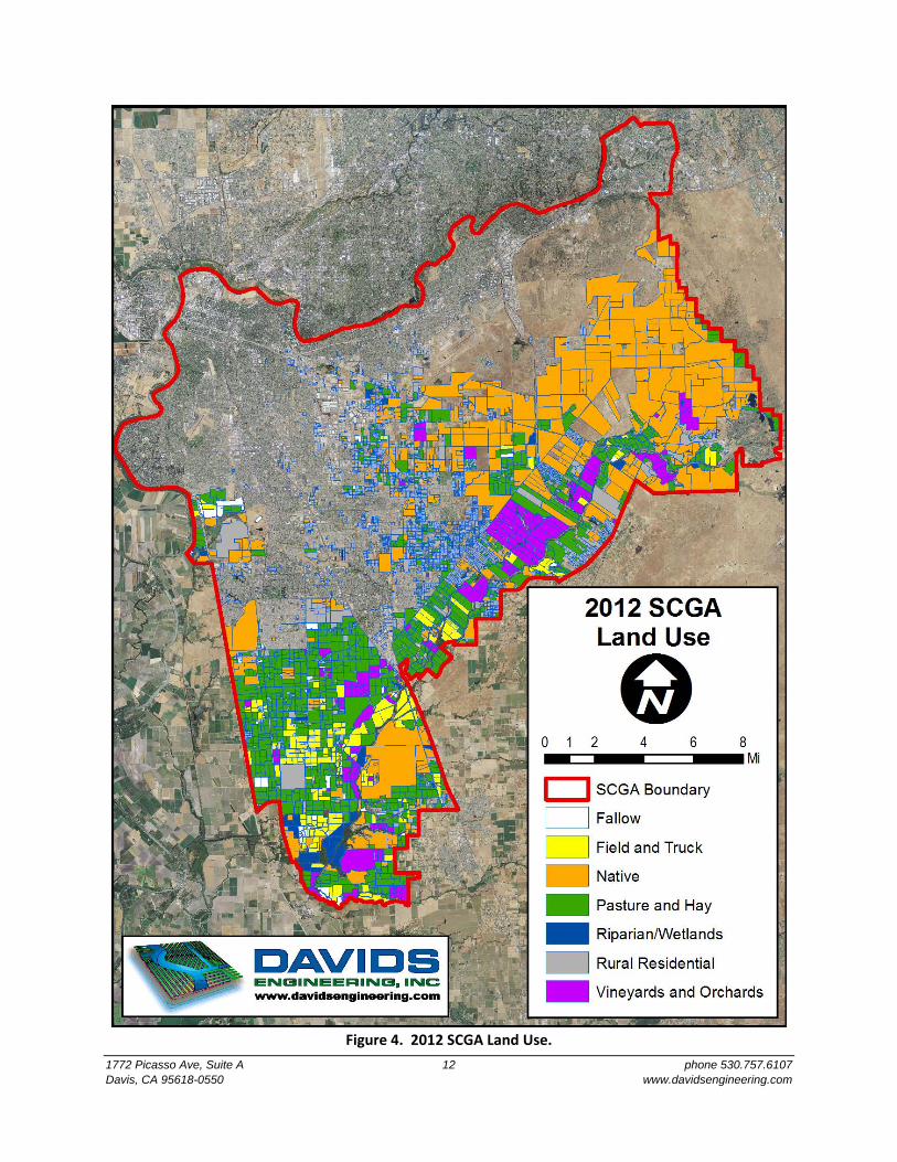
LandUseSummaryResults of the land use analysis are presented in Table 3, Figure 3, and Figure 4. Table 3 presents

estimated acreages by year for each land use class. 2011 and 2012 land use conditions are shown in

Figure 3 and Figure 4, respectively. The combined percent change for agricultural land uses, other than

fallow was less than one percent. In general, acreages for cropland other than pasture and hay

decreased from 2011 to 2012. For non‐crop land use classes, acreage remained nearly the same, with

an increase in acreage for Riparian/Wetlands resulting from development of managed wetlands on lands

previously cropped north of Thornton in the southwest corner of SCGA.


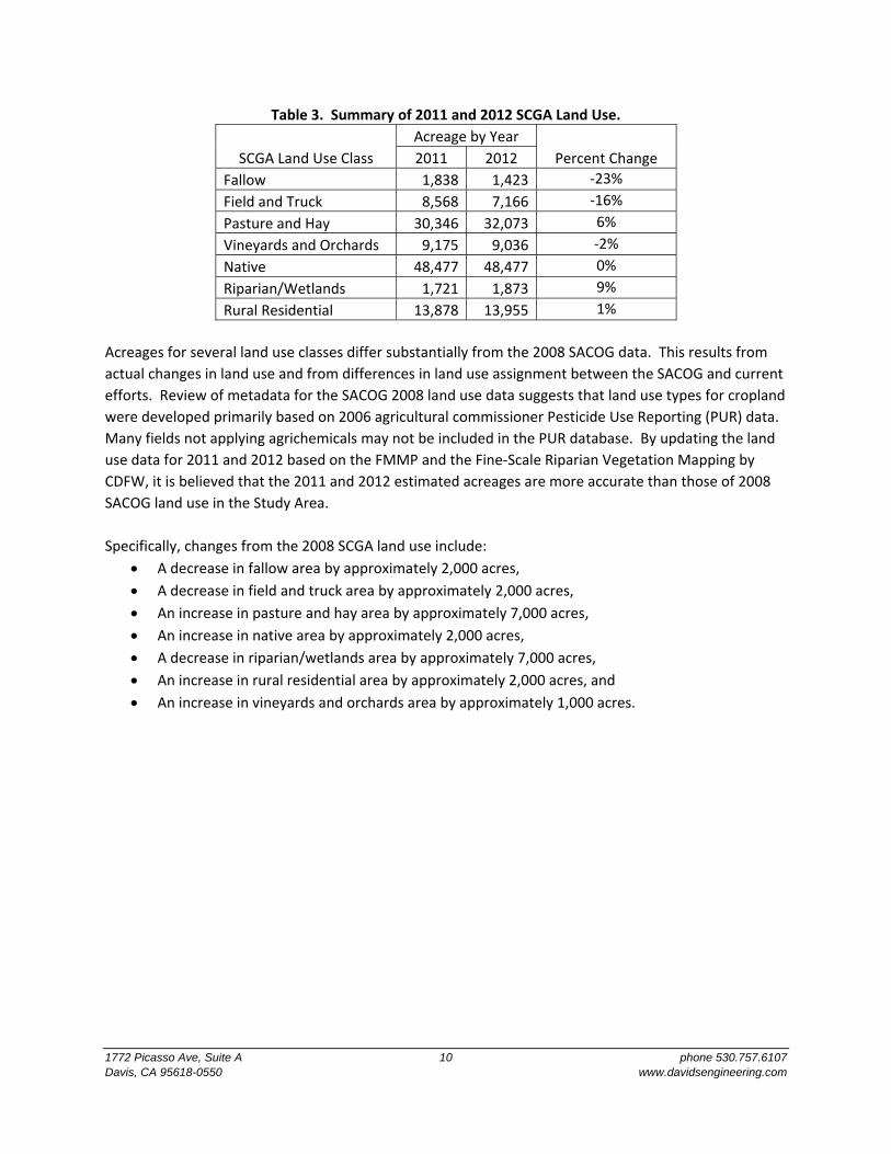
Table 3. Summary of 2011 and 2012 SCGA Land Use.

SCGA Land Use Class

Acreage by Year

Percent Change 2011 2012

Fallow 1,838 1,423 ‐23%

Field and Truck 8,568 7,166 ‐16%

Pasture and Hay 30,346 32,073 6%

Vineyards and Orchards 9,175 9,036 ‐2%

Native 48,477 48,477 0%

Riparian/Wetlands 1,721 1,873 9%

Rural Residential 13,878 13,955 1%

Acreages for several land use classes differ substantially from the 2008 SACOG data. This results from

actual changes in land use and from differences in land use assignment between the SACOG and current

efforts. Review of metadata for the SACOG 2008 land use data suggests that land use types for cropland

were developed primarily based on 2006 agricultural commissioner Pesticide Use Reporting (PUR) data.

Many fields not applying agrichemicals may not be included in the PUR database. By updating the land

use data for 2011 and 2012 based on the FMMP and the Fine‐Scale Riparian Vegetation Mapping by

CDFW, it is believed that the 2011 and 2012 estimated acreages are more accurate than those of 2008

SACOG land use in the Study Area.

Specifically, changes from the 2008 SCGA land use include:

A decrease in fallow area by approximately 2,000 acres,

A decrease in field and truck area by approximately 2,000 acres,

An increase in pasture and hay area by approximately 7,000 acres,

An increase in native area by approximately 2,000 acres,

A decrease in riparian/wetlands area by approximately 7,000 acres,

An increase in rural residential area by approximately 2,000 acres, and

An increase in vineyards and orchards area by approximately 1,000 acres.


Figure 3. 2011 SCGA Land Use.


Figure 4. 2012 SCGA Land Use.


ParameterizationofIWFMDemandCalculatorandAgriculturalWaterDemandEstimates

This section describes parameters used for IWFM Demand Calculator and agricultural water demand

estimates in the SCGA study area.

DevelopmentofETEstimatesCrop consumptive use or evapotranspiration (ET) was estimated using a crop coefficient‐reference

evapotranspiration calculation approach as described by Allen et al. (1998). In this approach, time‐

varying crop‐specific coefficients describing crop ET relative to grass reference ET are estimated and

multiplied by reference ET (ETo) from an agronomic weather station to calculate ET for each crop over

time. This section describes the analysis to develop time varying ET estimates by agricultural land use

class (including rural residential) through the development of a quality‐controlled reference ET time

series for 2011 – 2012 as well as crop coefficients representing actual ET rates in the Study Area.

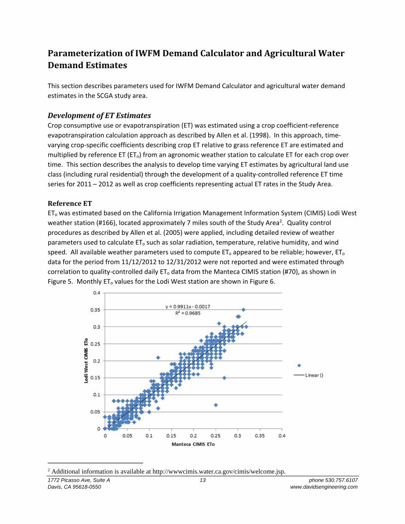
ReferenceETETo was estimated based on the California Irrigation Management Information System (CIMIS) Lodi West

weather station (#166), located approximately 7 miles south of the Study Area2. Quality control

procedures as described by Allen et al. (2005) were applied, including detailed review of weather

parameters used to calculate ETo such as solar radiation, temperature, relative humidity, and wind

speed. All available weather parameters used to compute ETo appeared to be reliable; however, ETo

data for the period from 11/12/2012 to 12/31/2012 were not reported and were estimated through

correlation to quality‐controlled daily ETo data from the Manteca CIMIS station (#70), as shown in

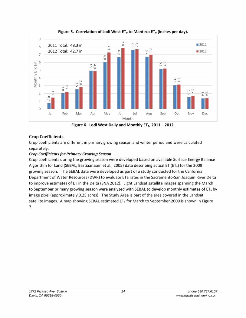
Figure 5. Monthly ETo values for the Lodi West station are shown in Figure 6.

2 Additional information is available at http://wwwcimis.water.ca.gov/cimis/welcome.jsp.


Figure 5. Correlation of Lodi West ETo to Manteca ETo (inches per day).

Figure 6. Lodi West Daily and Monthly ETo, 2011 – 2012.

CropCoefficientsCrop coefficients are different in primary growing season and winter period and were calculated

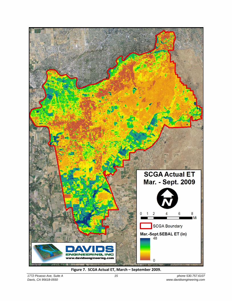
separately. CropCoefficientsforPrimaryGrowingSeasonCrop coefficients during the growing season were developed based on available Surface Energy Balance

Algorithm for Land (SEBAL, Bastiaanssen et al., 2005) data describing actual ET (ETa) for the 2009

growing season. The SEBAL data were developed as part of a study conducted for the California

Department of Water Resources (DWR) to evaluate ETa rates in the Sacramento‐San Joaquin River Delta

to improve estimates of ET in the Delta (SNA 2012). Eight Landsat satellite images spanning the March

to September primary growing season were analyzed with SEBAL to develop monthly estimates of ETa by

image pixel (approximately 0.25 acres). The Study Area is part of the area covered in the Landsat

satellite images. A map showing SEBAL estimated ETa for March to September 2009 is shown in Figure

7.

0.7

2.0

2.5

4.9

6.0

6.7

7.6

6.7

5.1

3.1

1.5 1.4

1.5

2.2

2.8

4.9

7.3

7.8 7.7

7.0

5.2

3.1

1.7 1.4

0

1

2

3

4

5

6

7

8

9

Jan Feb Mar Apr May Jun Jul Aug Sep Oct Nov Dec

Monthly ETo

(in)

Month

2011

2012

2011 Total: 48.3 in 2012 Total: 42.7 in


Figure 7. SCGA Actual ET, March – September 2009.


Cropping for each field polygon in 2009 was estimated based on the 2009 CDL. For field polygons with

fixed land use, as described in the previous section, the fixed land use was used. For the remaining field

polygons, the major SCGA land use class identified for each field polygon was assigned.

Average monthly ETa was extracted for each field polygon. Then, monthly crop coefficients for each

SCGA land use class were calculated for each month on a field‐by‐field basis dividing total ETa by the

total ETo from the Lodi West CIMIS station.

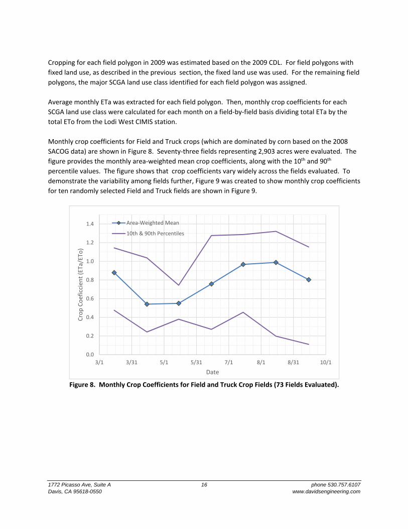
Monthly crop coefficients for Field and Truck crops (which are dominated by corn based on the 2008

SACOG data) are shown in Figure 8. Seventy‐three fields representing 2,903 acres were evaluated. The

figure provides the monthly area‐weighted mean crop coefficients, along with the 10th and 90th

percentile values. The figure shows that crop coefficients vary widely across the fields evaluated. To

demonstrate the variability among fields further, Figure 9 was created to show monthly crop coefficients

for ten randomly selected Field and Truck fields are shown in Figure 9.

Figure 8. Monthly Crop Coefficients for Field and Truck Crop Fields (73 Fields Evaluated).

0.0

0.2

0.4

0.6

0.8

1.0

1.2

1.4

3/1 3/31 5/1 5/31 7/1 8/1 8/31 10/1

Crop Coeficcien

t (ETa/ETo

)

Date

Area‐Weighted Mean

10th & 90th Percentiles


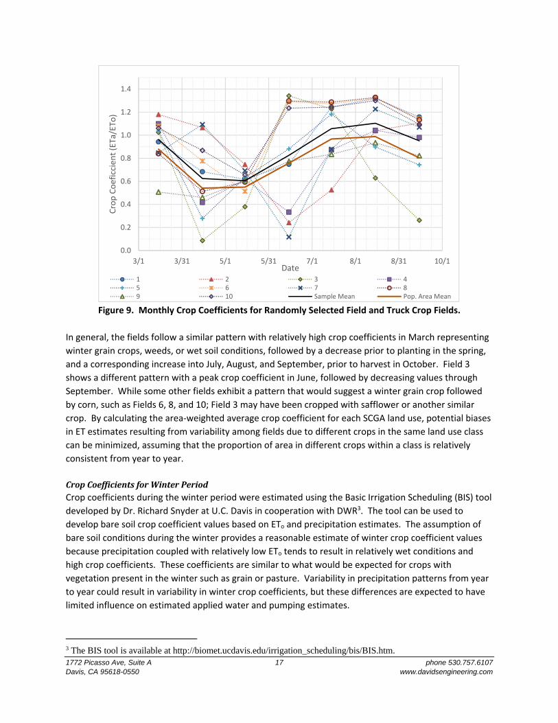
Figure 9. Monthly Crop Coefficients for Randomly Selected Field and Truck Crop Fields.

In general, the fields follow a similar pattern with relatively high crop coefficients in March representing

winter grain crops, weeds, or wet soil conditions, followed by a decrease prior to planting in the spring,

and a corresponding increase into July, August, and September, prior to harvest in October. Field 3

shows a different pattern with a peak crop coefficient in June, followed by decreasing values through

September. While some other fields exhibit a pattern that would suggest a winter grain crop followed

by corn, such as Fields 6, 8, and 10; Field 3 may have been cropped with safflower or another similar

crop. By calculating the area‐weighted average crop coefficient for each SCGA land use, potential biases

in ET estimates resulting from variability among fields due to different crops in the same land use class

can be minimized, assuming that the proportion of area in different crops within a class is relatively

consistent from year to year.

CropCoefficientsforWinterPeriodCrop coefficients during the winter period were estimated using the Basic Irrigation Scheduling (BIS) tool

developed by Dr. Richard Snyder at U.C. Davis in cooperation with DWR3. The tool can be used to

develop bare soil crop coefficient values based on ETo and precipitation estimates. The assumption of

bare soil conditions during the winter provides a reasonable estimate of winter crop coefficient values

because precipitation coupled with relatively low ETo tends to result in relatively wet conditions and

high crop coefficients. These coefficients are similar to what would be expected for crops with

vegetation present in the winter such as grain or pasture. Variability in precipitation patterns from year

to year could result in variability in winter crop coefficients, but these differences are expected to have

limited influence on estimated applied water and pumping estimates.

3 The BIS tool is available at http://biomet.ucdavis.edu/irrigation_scheduling/bis/BIS.htm.

0.0

0.2

0.4

0.6

0.8

1.0

1.2

1.4

3/1 3/31 5/1 5/31 7/1 8/1 8/31 10/1

Crop Coeficcien

t (ETa/ETo

)

Date1 2 3 45 6 7 89 10 Sample Mean Pop. Area Mean


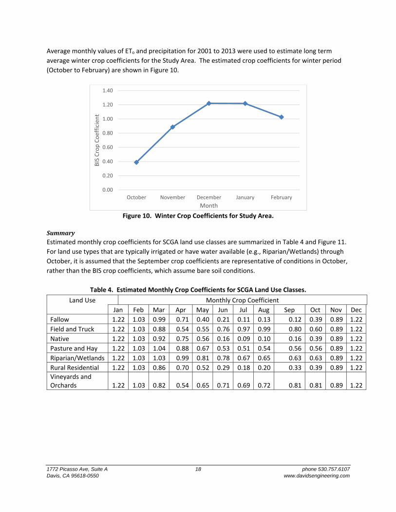
Average monthly values of ETo and precipitation for 2001 to 2013 were used to estimate long term

average winter crop coefficients for the Study Area. The estimated crop coefficients for winter period

(October to February) are shown in Figure 10.

Figure 10. Winter Crop Coefficients for Study Area.

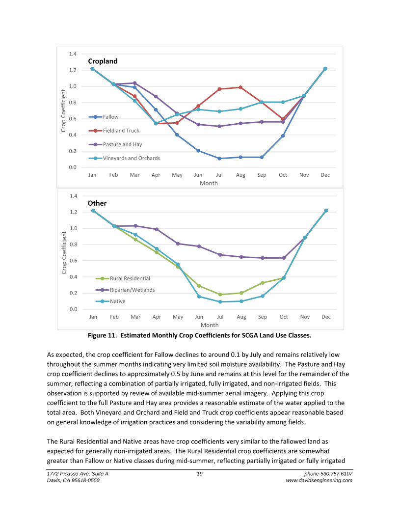
SummaryEstimated monthly crop coefficients for SCGA land use classes are summarized in Table 4 and Figure 11.

For land use types that are typically irrigated or have water available (e.g., Riparian/Wetlands) through

October, it is assumed that the September crop coefficients are representative of conditions in October,

rather than the BIS crop coefficients, which assume bare soil conditions.

Table 4. Estimated Monthly Crop Coefficients for SCGA Land Use Classes.

Land Use Monthly Crop Coefficient


Fallow 1.22 1.03 0.99 0.71 0.40 0.21 0.11 0.13 0.12 0.39 0.89 1.22

Field and Truck 1.22 1.03 0.88 0.54 0.55 0.76 0.97 0.99 0.80 0.60 0.89 1.22

Native 1.22 1.03 0.92 0.75 0.56 0.16 0.09 0.10 0.16 0.39 0.89 1.22

Pasture and Hay 1.22 1.03 1.04 0.88 0.67 0.53 0.51 0.54 0.56 0.56 0.89 1.22

Riparian/Wetlands 1.22 1.03 1.03 0.99 0.81 0.78 0.67 0.65 0.63 0.63 0.89 1.22

Rural Residential 1.22 1.03 0.86 0.70 0.52 0.29 0.18 0.20 0.33 0.39 0.89 1.22

Vineyards and Orchards 1.22 1.03 0.82 0.54 0.65 0.71 0.69 0.72 0.81 0.81 0.89 1.22

0.00

0.20

0.40

0.60

0.80

1.00

1.20

1.40

October November December January February

BIS Crop Coefficien

t

Month


Figure 11. Estimated Monthly Crop Coefficients for SCGA Land Use Classes.

As expected, the crop coefficient for Fallow declines to around 0.1 by July and remains relatively low

throughout the summer months indicating very limited soil moisture availability. The Pasture and Hay

crop coefficient declines to approximately 0.5 by June and remains at this level for the remainder of the

summer, reflecting a combination of partially irrigated, fully irrigated, and non‐irrigated fields. This

observation is supported by review of available mid‐summer aerial imagery. Applying this crop

coefficient to the full Pasture and Hay area provides a reasonable estimate of the water applied to the

total area. Both Vineyard and Orchard and Field and Truck crop coefficients appear reasonable based

on general knowledge of irrigation practices and considering the variability among fields.

The Rural Residential and Native areas have crop coefficients very similar to the fallowed land as

expected for generally non‐irrigated areas. The Rural Residential crop coefficients are somewhat

greater than Fallow or Native classes during mid‐summer, reflecting partially irrigated or fully irrigated

0.0

0.2

0.4

0.6

0.8

1.0

1.2

1.4


Crop Coefficien

t

Month

Fallow

Field and Truck

Pasture and Hay

Vineyards and Orchards

0.0

0.2

0.4

0.6

0.8

1.0

1.2

1.4


Crop Coefficien

t

Month

Rural Residential

Riparian/Wetlands

Native

Cropland

Other


parcels. The Riparian/Wetlands crop coefficient indicates increased water availability as compared to

Native areas, which consist primarily of annual grasslands, due to the access of riparian and wetland

vegetation to shallow groundwater and potentially some runoff (if any) from upgradient lands.

Availability of moisture declines over the course of the growing season, as indicated by decreasing crop

coefficients.

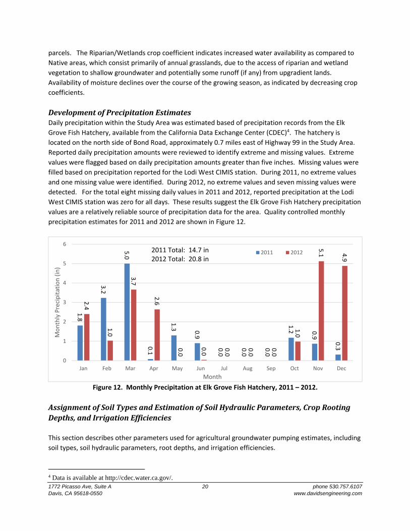
DevelopmentofPrecipitationEstimatesDaily precipitation within the Study Area was estimated based of precipitation records from the Elk

Grove Fish Hatchery, available from the California Data Exchange Center (CDEC)4. The hatchery is

located on the north side of Bond Road, approximately 0.7 miles east of Highway 99 in the Study Area.

Reported daily precipitation amounts were reviewed to identify extreme and missing values. Extreme

values were flagged based on daily precipitation amounts greater than five inches. Missing values were

filled based on precipitation reported for the Lodi West CIMIS station. During 2011, no extreme values

and one missing value were identified. During 2012, no extreme values and seven missing values were

detected. For the total eight missing daily values in 2011 and 2012, reported precipitation at the Lodi

West CIMIS station was zero for all days. These results suggest the Elk Grove Fish Hatchery precipitation

values are a relatively reliable source of precipitation data for the area. Quality controlled monthly

precipitation estimates for 2011 and 2012 are shown in Figure 12.

Figure 12. Monthly Precipitation at Elk Grove Fish Hatchery, 2011 – 2012.

AssignmentofSoilTypesandEstimationofSoilHydraulicParameters,CropRootingDepths,andIrrigationEfficiencies

This section describes other parameters used for agricultural groundwater pumping estimates, including

soil types, soil hydraulic parameters, root depths, and irrigation efficiencies.

4 Data is available at http://cdec.water.ca.gov/.

1.8

3.2

5.0

0.1

1.3 0

.9

0.0

0.0

0.0

1.2 0.9

0.3

2.4

1.0

3.7

2.6

0.0

0.0

0.0

0.0

0.0

1.0

5.1 4.9

0

1

2

3

4

5

6


Monthly Precipitation (in)

Month

2011 20122011 Total: 14.7 in2012 Total: 20.8 in


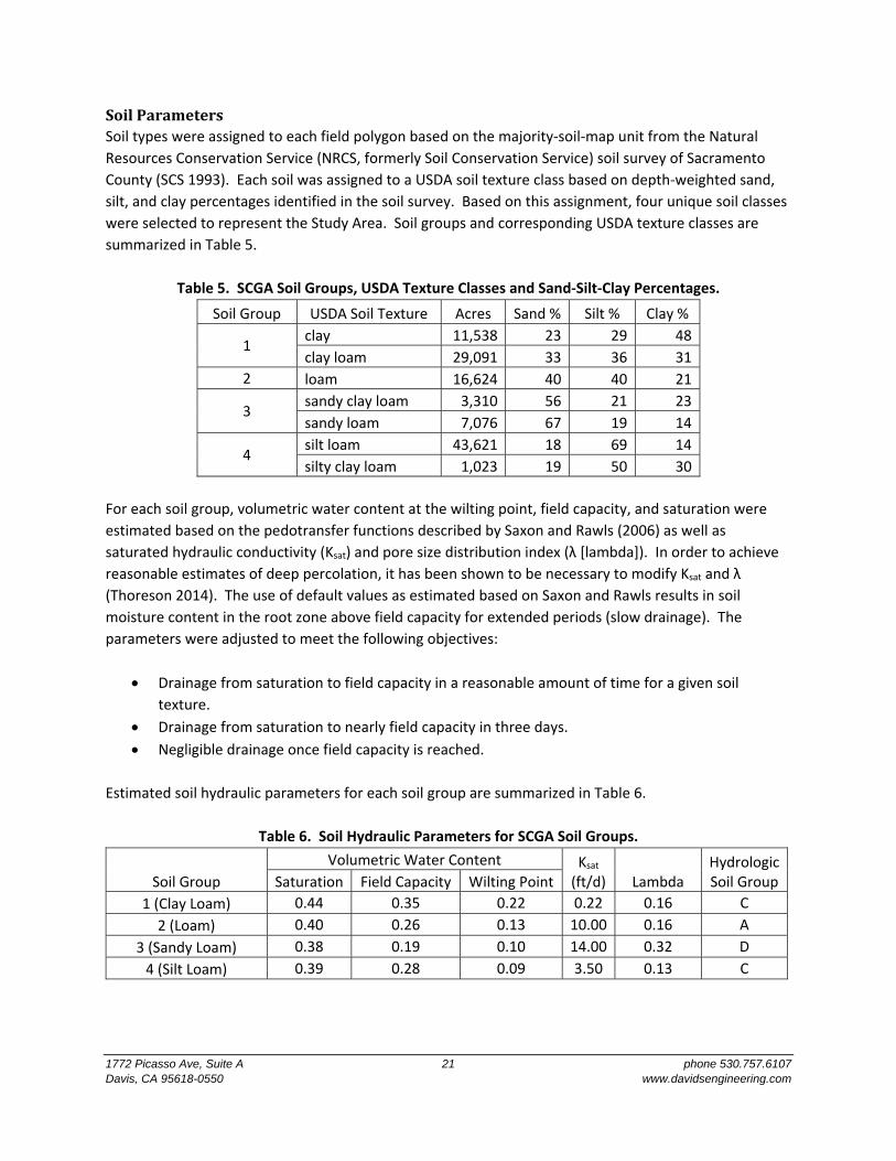
SoilParametersSoil types were assigned to each field polygon based on the majority‐soil‐map unit from the Natural

Resources Conservation Service (NRCS, formerly Soil Conservation Service) soil survey of Sacramento

County (SCS 1993). Each soil was assigned to a USDA soil texture class based on depth‐weighted sand,

silt, and clay percentages identified in the soil survey. Based on this assignment, four unique soil classes

were selected to represent the Study Area. Soil groups and corresponding USDA texture classes are

summarized in Table 5.

Table 5. SCGA Soil Groups, USDA Texture Classes and Sand‐Silt‐Clay Percentages.

Soil Group USDA Soil Texture Acres Sand % Silt % Clay %

1 clay 11,538 23 29 48

clay loam 29,091 33 36 31

2 loam 16,624 40 40 21

3 sandy clay loam 3,310 56 21 23

sandy loam 7,076 67 19 14

4 silt loam 43,621 18 69 14

silty clay loam 1,023 19 50 30

For each soil group, volumetric water content at the wilting point, field capacity, and saturation were

estimated based on the pedotransfer functions described by Saxon and Rawls (2006) as well as

saturated hydraulic conductivity (Ksat) and pore size distribution index (λ [lambda]). In order to achieve

reasonable estimates of deep percolation, it has been shown to be necessary to modify Ksat and λ

(Thoreson 2014). The use of default values as estimated based on Saxon and Rawls results in soil

moisture content in the root zone above field capacity for extended periods (slow drainage). The

parameters were adjusted to meet the following objectives:

Drainage from saturation to field capacity in a reasonable amount of time for a given soil

texture.

Drainage from saturation to nearly field capacity in three days.

Negligible drainage once field capacity is reached.

Estimated soil hydraulic parameters for each soil group are summarized in Table 6.

Table 6. Soil Hydraulic Parameters for SCGA Soil Groups.

Soil Group

Volumetric Water Content Ksat (ft/d) Lambda

Hydrologic Soil Group Saturation Field Capacity Wilting Point

1 (Clay Loam) 0.44 0.35 0.22 0.22 0.16 C

2 (Loam) 0.40 0.26 0.13 10.00 0.16 A

3 (Sandy Loam) 0.38 0.19 0.10 14.00 0.32 D

4 (Silt Loam) 0.39 0.28 0.09 3.50 0.13 C


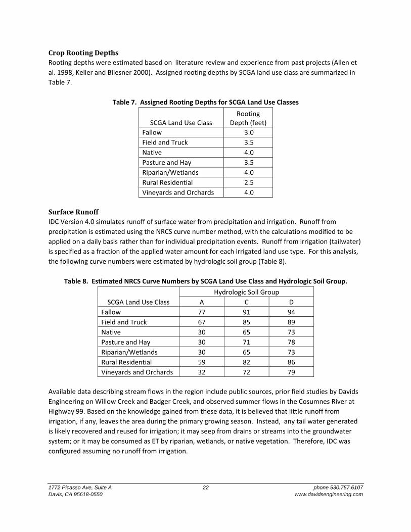
CropRootingDepthsRooting depths were estimated based on literature review and experience from past projects (Allen et

al. 1998, Keller and Bliesner 2000). Assigned rooting depths by SCGA land use class are summarized in

Table 7.

Table 7. Assigned Rooting Depths for SCGA Land Use Classes

SCGA Land Use Class Rooting

Depth (feet)

Fallow 3.0

Field and Truck 3.5

Native 4.0

Pasture and Hay 3.5

Riparian/Wetlands 4.0

Rural Residential 2.5

Vineyards and Orchards 4.0

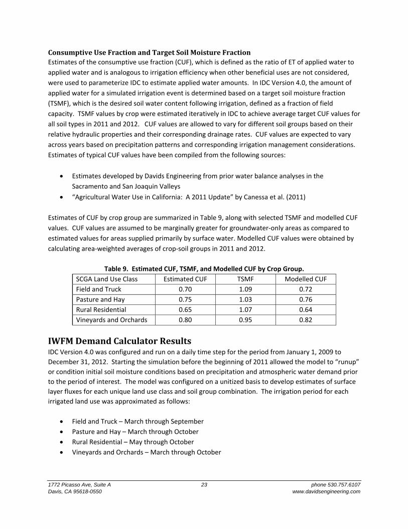
SurfaceRunoffIDC Version 4.0 simulates runoff of surface water from precipitation and irrigation. Runoff from

precipitation is estimated using the NRCS curve number method, with the calculations modified to be

applied on a daily basis rather than for individual precipitation events. Runoff from irrigation (tailwater)

is specified as a fraction of the applied water amount for each irrigated land use type. For this analysis,

the following curve numbers were estimated by hydrologic soil group (Table 8).

Table 8. Estimated NRCS Curve Numbers by SCGA Land Use Class and Hydrologic Soil Group.

SCGA Land Use Class

Hydrologic Soil Group

A C D

Fallow 77 91 94

Field and Truck 67 85 89

Native 30 65 73

Pasture and Hay 30 71 78

Riparian/Wetlands 30 65 73

Rural Residential 59 82 86

Vineyards and Orchards 32 72 79

Available data describing stream flows in the region include public sources, prior field studies by Davids

Engineering on Willow Creek and Badger Creek, and observed summer flows in the Cosumnes River at

Highway 99. Based on the knowledge gained from these data, it is believed that little runoff from

irrigation, if any, leaves the area during the primary growing season. Instead, any tail water generated

is likely recovered and reused for irrigation; it may seep from drains or streams into the groundwater

system; or it may be consumed as ET by riparian, wetlands, or native vegetation. Therefore, IDC was

configured assuming no runoff from irrigation.


ConsumptiveUseFractionandTargetSoilMoistureFractionEstimates of the consumptive use fraction (CUF), which is defined as the ratio of ET of applied water to

applied water and is analogous to irrigation efficiency when other beneficial uses are not considered,

were used to parameterize IDC to estimate applied water amounts. In IDC Version 4.0, the amount of

applied water for a simulated irrigation event is determined based on a target soil moisture fraction

(TSMF), which is the desired soil water content following irrigation, defined as a fraction of field

capacity. TSMF values by crop were estimated iteratively in IDC to achieve average target CUF values for

all soil types in 2011 and 2012. CUF values are allowed to vary for different soil groups based on their

relative hydraulic properties and their corresponding drainage rates. CUF values are expected to vary

across years based on precipitation patterns and corresponding irrigation management considerations.

Estimates of typical CUF values have been compiled from the following sources:

Estimates developed by Davids Engineering from prior water balance analyses in the

Sacramento and San Joaquin Valleys

“Agricultural Water Use in California: A 2011 Update” by Canessa et al. (2011)

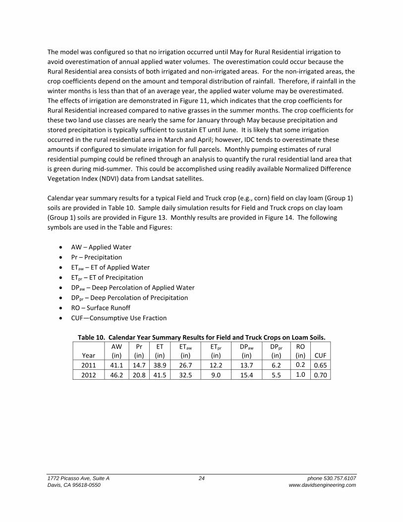
Estimates of CUF by crop group are summarized in Table 9, along with selected TSMF and modelled CUF

values. CUF values are assumed to be marginally greater for groundwater‐only areas as compared to

estimated values for areas supplied primarily by surface water. Modelled CUF values were obtained by

calculating area‐weighted averages of crop‐soil groups in 2011 and 2012.

Table 9. Estimated CUF, TSMF, and Modelled CUF by Crop Group.

SCGA Land Use Class Estimated CUF TSMF Modelled CUF

Field and Truck 0.70 1.09 0.72

Pasture and Hay 0.75 1.03 0.76

Rural Residential 0.65 1.07 0.64

Vineyards and Orchards 0.80 0.95 0.82

IWFMDemandCalculatorResultsIDC Version 4.0 was configured and run on a daily time step for the period from January 1, 2009 to

December 31, 2012. Starting the simulation before the beginning of 2011 allowed the model to “runup”

or condition initial soil moisture conditions based on precipitation and atmospheric water demand prior

to the period of interest. The model was configured on a unitized basis to develop estimates of surface

layer fluxes for each unique land use class and soil group combination. The irrigation period for each

irrigated land use was approximated as follows:

Field and Truck – March through September

Pasture and Hay – March through October

Rural Residential – May through October

Vineyards and Orchards – March through October


The model was configured so that no irrigation occurred until May for Rural Residential irrigation to

avoid overestimation of annual applied water volumes. The overestimation could occur because the

Rural Residential area consists of both irrigated and non‐irrigated areas. For the non‐irrigated areas, the

crop coefficients depend on the amount and temporal distribution of rainfall. Therefore, if rainfall in the

winter months is less than that of an average year, the applied water volume may be overestimated.

The effects of irrigation are demonstrated in Figure 11, which indicates that the crop coefficients for

Rural Residential increased compared to native grasses in the summer months. The crop coefficients for

these two land use classes are nearly the same for January through May because precipitation and

stored precipitation is typically sufficient to sustain ET until June. It is likely that some irrigation

occurred in the rural residential area in March and April; however, IDC tends to overestimate these

amounts if configured to simulate irrigation for full parcels. Monthly pumping estimates of rural

residential pumping could be refined through an analysis to quantify the rural residential land area that

is green during mid‐summer. This could be accomplished using readily available Normalized Difference

Vegetation Index (NDVI) data from Landsat satellites.

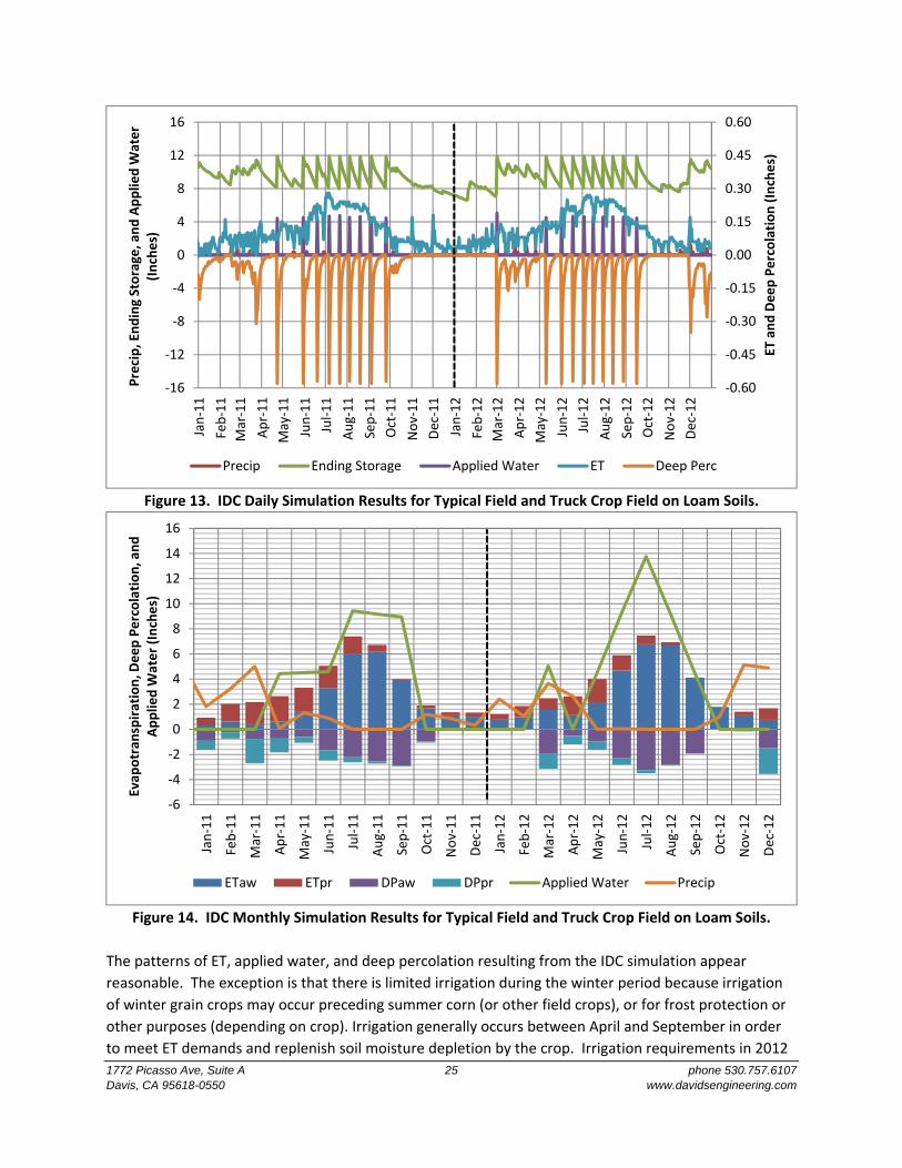
Calendar year summary results for a typical Field and Truck crop (e.g., corn) field on clay loam (Group 1)

soils are provided in Table 10. Sample daily simulation results for Field and Truck crops on clay loam

(Group 1) soils are provided in Figure 13. Monthly results are provided in Figure 14. The following

symbols are used in the Table and Figures:

AW – Applied Water

Pr – Precipitation

ETaw – ET of Applied Water

ETpr – ET of Precipitation

DPaw – Deep Percolation of Applied Water

DPpr – Deep Percolation of Precipitation

RO – Surface Runoff

CUF—Consumptive Use Fraction

Table 10. Calendar Year Summary Results for Field and Truck Crops on Loam Soils.

Year AW (in)

Pr (in)

ET (in)

ETaw (in)

ETpr (in)

DPaw (in)

DPpr (in)

RO (in) CUF

2011 41.1 14.7 38.9 26.7 12.2 13.7 6.2 0.2 0.65

2012 46.2 20.8 41.5 32.5 9.0 15.4 5.5 1.0 0.70


Figure 13. IDC Daily Simulation Results for Typical Field and Truck Crop Field on Loam Soils.

Figure 14. IDC Monthly Simulation Results for Typical Field and Truck Crop Field on Loam Soils.

The patterns of ET, applied water, and deep percolation resulting from the IDC simulation appear

reasonable. The exception is that there is limited irrigation during the winter period because irrigation

of winter grain crops may occur preceding summer corn (or other field crops), or for frost protection or

other purposes (depending on crop). Irrigation generally occurs between April and September in order

to meet ET demands and replenish soil moisture depletion by the crop. Irrigation requirements in 2012

‐0.60

‐0.45

‐0.30

‐0.15

0.00

0.15

0.30

0.45

0.60

‐16

‐12

‐8

‐4

0

4

8

12

16

Jan‐11

Feb‐11

Mar‐11

Apr‐11

May‐11

Jun‐11

Jul‐11

Aug‐11

Sep‐11

Oct‐11

Nov‐11

Dec‐11

Jan‐12

Feb‐12

Mar‐12

Apr‐12

May‐12

Jun‐12

Jul‐12

Aug‐12

Sep‐12

Oct‐12

Nov‐12

Dec‐12

ET and Deep Percolation (Inches)

Precip, Ending Storage, and Applied W

ater

(Inches)

Precip Ending Storage Applied Water ET Deep Perc

‐6

‐4

‐2

0

2

4

6

8

10

12

14

16

Jan‐11

Feb‐11

Mar‐11

Apr‐11

May‐11

Jun‐11

Jul‐11

Aug‐11

Sep‐11

Oct‐11

Nov‐11

Dec‐11

Jan‐12

Feb‐12

Mar‐12

Apr‐12

May‐12

Jun‐12

Jul‐12

Aug‐12

Sep‐12

Oct‐12

Nov‐12

Dec‐12

Evap

otran

spiration, D

eep Percolation, and

Applied W

ater (Inches)

ETaw ETpr DPaw DPpr Applied Water Precip


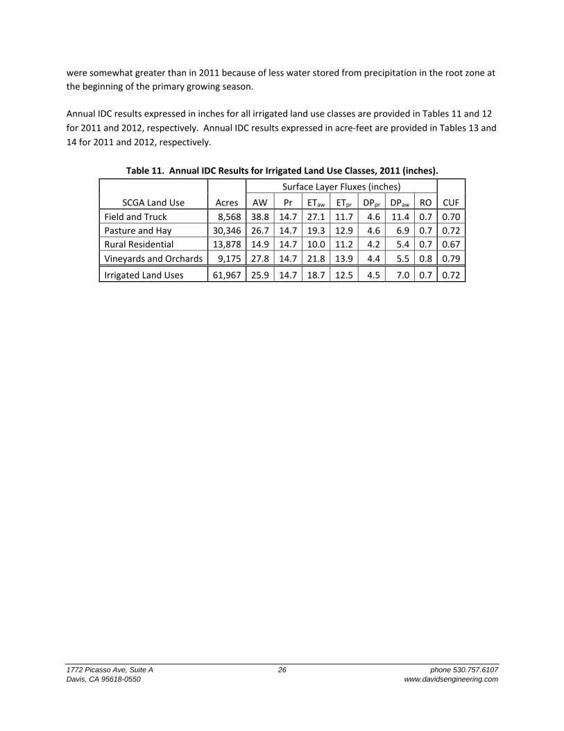
were somewhat greater than in 2011 because of less water stored from precipitation in the root zone at

the beginning of the primary growing season.

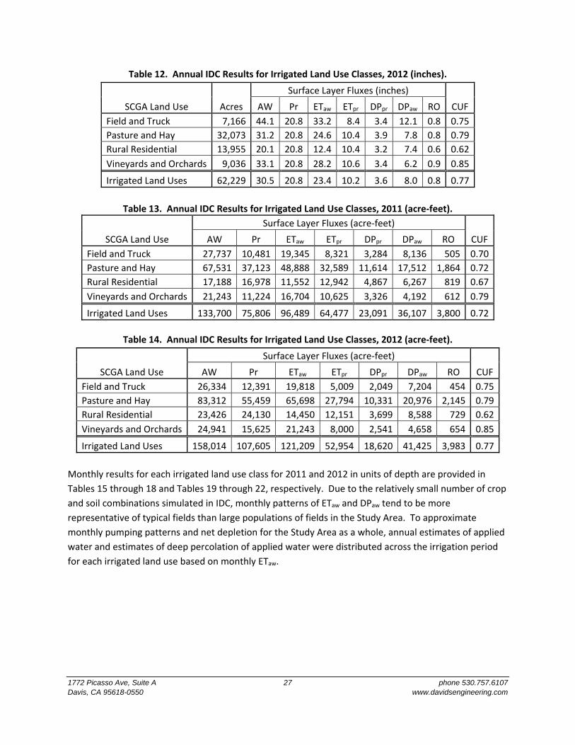
Annual IDC results expressed in inches for all irrigated land use classes are provided in Tables 11 and 12

for 2011 and 2012, respectively. Annual IDC results expressed in acre‐feet are provided in Tables 13 and

14 for 2011 and 2012, respectively.

Table 11. Annual IDC Results for Irrigated Land Use Classes, 2011 (inches).

SCGA Land Use Acres

Surface Layer Fluxes (inches)

CUF AW Pr ETaw ETpr DPpr DPaw RO

Field and Truck 8,568 38.8 14.7 27.1 11.7 4.6 11.4 0.7 0.70

Pasture and Hay 30,346 26.7 14.7 19.3 12.9 4.6 6.9 0.7 0.72

Rural Residential 13,878 14.9 14.7 10.0 11.2 4.2 5.4 0.7 0.67

Vineyards and Orchards 9,175 27.8 14.7 21.8 13.9 4.4 5.5 0.8 0.79

Irrigated Land Uses 61,967 25.9 14.7 18.7 12.5 4.5 7.0 0.7 0.72


Table 12. Annual IDC Results for Irrigated Land Use Classes, 2012 (inches).

SCGA Land Use Acres



Field and Truck 7,166 44.1 20.8 33.2 8.4 3.4 12.1 0.8 0.75

Pasture and Hay 32,073 31.2 20.8 24.6 10.4 3.9 7.8 0.8 0.79

Rural Residential 13,955 20.1 20.8 12.4 10.4 3.2 7.4 0.6 0.62

Vineyards and Orchards 9,036 33.1 20.8 28.2 10.6 3.4 6.2 0.9 0.85

Irrigated Land Uses 62,229 30.5 20.8 23.4 10.2 3.6 8.0 0.8 0.77

Table 13. Annual IDC Results for Irrigated Land Use Classes, 2011 (acre‐feet).

SCGA Land Use

Surface Layer Fluxes (acre‐feet)


Field and Truck 27,737 10,481 19,345 8,321 3,284 8,136 505 0.70

Pasture and Hay 67,531 37,123 48,888 32,589 11,614 17,512 1,864 0.72

Rural Residential 17,188 16,978 11,552 12,942 4,867 6,267 819 0.67

Vineyards and Orchards 21,243 11,224 16,704 10,625 3,326 4,192 612 0.79

Irrigated Land Uses 133,700 75,806 96,489 64,477 23,091 36,107 3,800 0.72

Table 14. Annual IDC Results for Irrigated Land Use Classes, 2012 (acre‐feet).

SCGA Land Use

Surface Layer Fluxes (acre‐feet)


Field and Truck 26,334 12,391 19,818 5,009 2,049 7,204 454 0.75

Pasture and Hay 83,312 55,459 65,698 27,794 10,331 20,976 2,145 0.79

Rural Residential 23,426 24,130 14,450 12,151 3,699 8,588 729 0.62

Vineyards and Orchards 24,941 15,625 21,243 8,000 2,541 4,658 654 0.85

Irrigated Land Uses 158,014 107,605 121,209 52,954 18,620 41,425 3,983 0.77

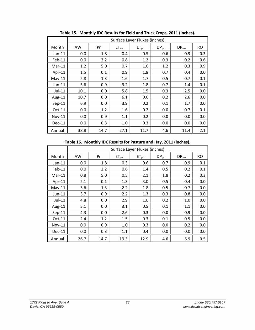
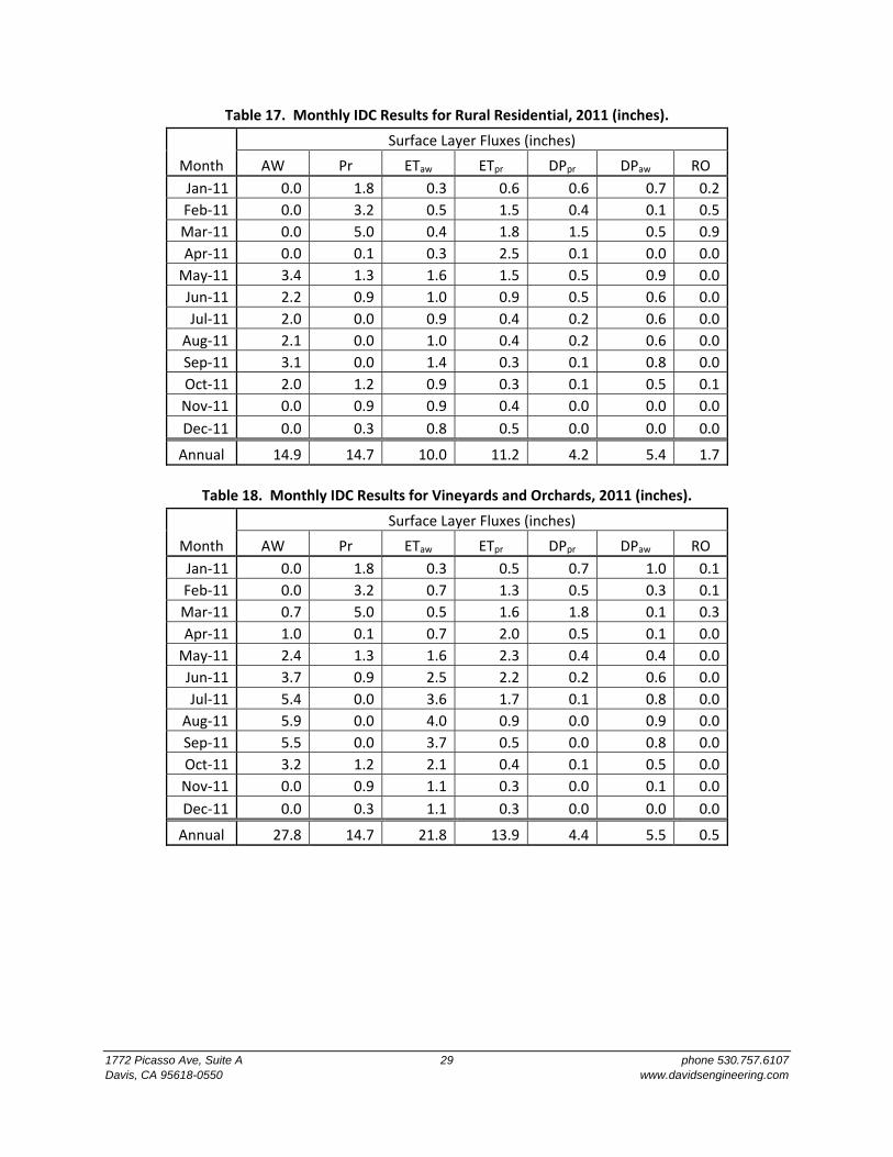
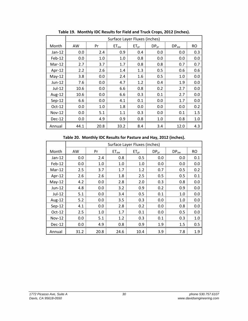
Monthly results for each irrigated land use class for 2011 and 2012 in units of depth are provided in

Tables 15 through 18 and Tables 19 through 22, respectively. Due to the relatively small number of crop

and soil combinations simulated in IDC, monthly patterns of ETaw and DPaw tend to be more

representative of typical fields than large populations of fields in the Study Area. To approximate

monthly pumping patterns and net depletion for the Study Area as a whole, annual estimates of applied

water and estimates of deep percolation of applied water were distributed across the irrigation period

for each irrigated land use based on monthly ETaw.


Table 15. Monthly IDC Results for Field and Truck Crops, 2011 (inches).

Month


AW Pr ETaw ETpr DPpr DPaw RO

Jan‐11 0.0 1.8 0.4 0.5 0.6 0.9 0.3

Feb‐11 0.0 3.2 0.8 1.2 0.3 0.2 0.6

Mar‐11 1.2 5.0 0.7 1.6 1.2 0.3 0.9

Apr‐11 1.5 0.1 0.9 1.8 0.7 0.4 0.0

May‐11 2.8 1.3 1.6 1.7 0.5 0.7 0.1

Jun‐11 5.6 0.9 3.2 1.8 0.7 1.4 0.1

Jul‐11 10.1 0.0 5.8 1.5 0.3 2.5 0.0

Aug‐11 10.7 0.0 6.1 0.6 0.2 2.6 0.0

Sep‐11 6.9 0.0 3.9 0.2 0.1 1.7 0.0

Oct‐11 0.0 1.2 1.6 0.2 0.0 0.7 0.1

Nov‐11 0.0 0.9 1.1 0.2 0.0 0.0 0.0

Dec‐11 0.0 0.3 1.0 0.3 0.0 0.0 0.0

Annual 38.8 14.7 27.1 11.7 4.6 11.4 2.1

Table 16. Monthly IDC Results for Pasture and Hay, 2011 (inches).

Month



Jan‐11 0.0 1.8 0.3 0.6 0.7 0.9 0.1

Feb‐11 0.0 3.2 0.6 1.4 0.5 0.2 0.1

Mar‐11 0.8 5.0 0.5 2.1 1.8 0.2 0.3

Apr‐11 2.1 0.1 1.3 3.0 0.5 0.4 0.0

May‐11 3.6 1.3 2.2 1.8 0.5 0.7 0.0

Jun‐11 3.7 0.9 2.2 1.3 0.3 0.8 0.0

Jul‐11 4.8 0.0 2.9 1.0 0.2 1.0 0.0

Aug‐11 5.1 0.0 3.1 0.5 0.1 1.1 0.0

Sep‐11 4.3 0.0 2.6 0.3 0.0 0.9 0.0

Oct‐11 2.4 1.2 1.5 0.3 0.1 0.5 0.0

Nov‐11 0.0 0.9 1.0 0.3 0.0 0.2 0.0

Dec‐11 0.0 0.3 1.1 0.4 0.0 0.0 0.0

Annual 26.7 14.7 19.3 12.9 4.6 6.9 0.5


Table 17. Monthly IDC Results for Rural Residential, 2011 (inches).

Month



Jan‐11 0.0 1.8 0.3 0.6 0.6 0.7 0.2

Feb‐11 0.0 3.2 0.5 1.5 0.4 0.1 0.5

Mar‐11 0.0 5.0 0.4 1.8 1.5 0.5 0.9

Apr‐11 0.0 0.1 0.3 2.5 0.1 0.0 0.0

May‐11 3.4 1.3 1.6 1.5 0.5 0.9 0.0

Jun‐11 2.2 0.9 1.0 0.9 0.5 0.6 0.0

Jul‐11 2.0 0.0 0.9 0.4 0.2 0.6 0.0

Aug‐11 2.1 0.0 1.0 0.4 0.2 0.6 0.0

Sep‐11 3.1 0.0 1.4 0.3 0.1 0.8 0.0

Oct‐11 2.0 1.2 0.9 0.3 0.1 0.5 0.1

Nov‐11 0.0 0.9 0.9 0.4 0.0 0.0 0.0

Dec‐11 0.0 0.3 0.8 0.5 0.0 0.0 0.0

Annual 14.9 14.7 10.0 11.2 4.2 5.4 1.7

Table 18. Monthly IDC Results for Vineyards and Orchards, 2011 (inches).

Month



Jan‐11 0.0 1.8 0.3 0.5 0.7 1.0 0.1

Feb‐11 0.0 3.2 0.7 1.3 0.5 0.3 0.1

Mar‐11 0.7 5.0 0.5 1.6 1.8 0.1 0.3

Apr‐11 1.0 0.1 0.7 2.0 0.5 0.1 0.0

May‐11 2.4 1.3 1.6 2.3 0.4 0.4 0.0

Jun‐11 3.7 0.9 2.5 2.2 0.2 0.6 0.0

Jul‐11 5.4 0.0 3.6 1.7 0.1 0.8 0.0

Aug‐11 5.9 0.0 4.0 0.9 0.0 0.9 0.0

Sep‐11 5.5 0.0 3.7 0.5 0.0 0.8 0.0

Oct‐11 3.2 1.2 2.1 0.4 0.1 0.5 0.0

Nov‐11 0.0 0.9 1.1 0.3 0.0 0.1 0.0

Dec‐11 0.0 0.3 1.1 0.3 0.0 0.0 0.0

Annual 27.8 14.7 21.8 13.9 4.4 5.5 0.5


Table 19. Monthly IDC Results for Field and Truck Crops, 2012 (inches).

Month



Jan‐12 0.0 2.4 0.9 0.4 0.0 0.0 0.3

Feb‐12 0.0 1.0 1.0 0.8 0.0 0.0 0.0

Mar‐12 2.7 3.7 1.7 0.8 0.8 0.7 0.7

Apr‐12 2.2 2.6 1.4 1.3 0.5 0.6 0.6

May‐12 3.8 0.0 2.4 1.6 0.5 1.0 0.0

Jun‐12 7.6 0.0 4.7 1.2 0.4 1.9 0.0

Jul‐12 10.6 0.0 6.6 0.8 0.2 2.7 0.0

Aug‐12 10.6 0.0 6.6 0.3 0.1 2.7 0.0

Sep‐12 6.6 0.0 4.1 0.1 0.0 1.7 0.0

Oct‐12 0.0 1.0 1.8 0.0 0.0 0.0 0.2

Nov‐12 0.0 5.1 1.1 0.3 0.0 0.1 1.5

Dec‐12 0.0 4.9 0.9 0.8 1.0 0.8 1.0

Annual 44.1 20.8 33.2 8.4 3.4 12.0 4.3

Table 20. Monthly IDC Results for Pasture and Hay, 2012 (inches).

Month



Jan‐12 0.0 2.4 0.8 0.5 0.0 0.0 0.1

Feb‐12 0.0 1.0 1.0 1.0 0.0 0.0 0.0

Mar‐12 2.5 3.7 1.7 1.2 0.7 0.5 0.2

Apr‐12 2.6 2.6 1.8 2.5 0.5 0.5 0.1

May‐12 4.2 0.0 2.8 2.0 0.3 0.8 0.0

Jun‐12 4.8 0.0 3.2 0.9 0.2 0.9 0.0

Jul‐12 5.1 0.0 3.4 0.5 0.1 1.0 0.0

Aug‐12 5.2 0.0 3.5 0.3 0.0 1.0 0.0

Sep‐12 4.1 0.0 2.8 0.2 0.0 0.8 0.0

Oct‐12 2.5 1.0 1.7 0.1 0.0 0.5 0.0

Nov‐12 0.0 5.1 1.2 0.3 0.1 0.3 1.0

Dec‐12 0.0 4.9 0.8 0.9 1.9 1.5 0.5

Annual 31.2 20.8 24.6 10.4 3.9 7.8 1.9


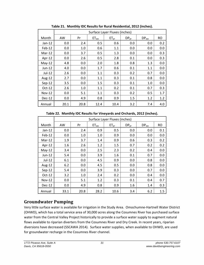
Table 21. Monthly IDC Results for Rural Residential, 2012 (inches).

Month



Jan‐12 0.0 2.4 0.5 0.6 0.0 0.0 0.2

Feb‐12 0.0 1.0 0.6 1.1 0.0 0.0 0.0

Mar‐12 0.0 3.7 0.5 1.3 0.0 0.0 0.3

Apr‐12 0.0 2.6 0.5 2.8 0.1 0.0 0.3

May‐12 4.8 0.0 2.0 1.8 0.8 1.3 0.0

Jun‐12 4.0 0.0 1.7 0.6 0.1 1.1 0.0

Jul‐12 2.6 0.0 1.1 0.3 0.2 0.7 0.0

Aug‐12 2.7 0.0 1.1 0.3 0.1 0.8 0.0

Sep‐12 3.5 0.0 1.5 0.3 0.1 1.0 0.0

Oct‐12 2.6 1.0 1.1 0.2 0.1 0.7 0.3

Nov‐12 0.0 5.1 1.1 0.3 0.2 0.5 1.7

Dec‐12 0.0 4.9 0.8 0.9 1.5 1.2 1.2

Annual 20.1 20.8 12.4 10.4 3.2 7.4 4.0

Table 22. Monthly IDC Results for Vineyards and Orchards, 2012 (inches).

Month



Jan‐12 0.0 2.4 0.9 0.5 0.0 0.0 0.1

Feb‐12 0.0 1.0 1.0 0.9 0.0 0.0 0.0

Mar‐12 1.9 3.7 1.4 0.9 0.6 0.3 0.2

Apr‐12 1.6 2.6 1.2 1.5 0.7 0.2 0.2

May‐12 3.4 0.0 2.5 2.3 0.2 0.4 0.0

Jun‐12 5.4 0.0 3.9 1.6 0.1 0.7 0.0

Jul‐12 6.1 0.0 4.5 0.9 0.0 0.8 0.0

Aug‐12 6.2 0.0 4.5 0.5 0.0 0.8 0.0

Sep‐12 5.4 0.0 3.9 0.3 0.0 0.7 0.0

Oct‐12 3.2 1.0 2.4 0.2 0.0 0.4 0.0

Nov‐12 0.0 5.1 1.2 0.3 0.1 0.4 0.7

Dec‐12 0.0 4.9 0.8 0.9 1.6 1.4 0.3

Annual 33.1 20.8 28.2 10.6 3.4 6.2 1.5

GroundwaterPumpingVery little surface water is available for irrigation in the Study Area. Omochumne‐Hartnell Water District

(OHWD), which has a total service area of 30,000 acres along the Cosumnes River has purchased surface

water from the Central Valley Project historically to provide a surface water supply to augment natural

flows available to riparian diverters from the Cosumnes River and Dry Creek. In recent years, riparian

diversions have decreased (SSCAWA 2014). Surface water supplies, when available to OHWD, are used

for groundwater recharge in the Cosumnes River channel.


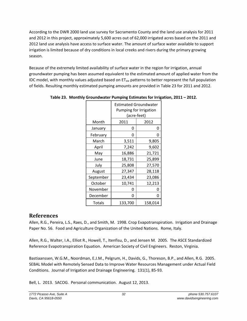
According to the DWR 2000 land use survey for Sacramento County and the land use analysis for 2011

and 2012 in this project, approximately 5,600 acres out of 62,000 irrigated acres based on the 2011 and

2012 land use analysis have access to surface water. The amount of surface water available to support

irrigation is limited because of dry conditions in local creeks and rivers during the primary growing

season.

Because of the extremely limited availability of surface water in the region for irrigation, annual

groundwater pumping has been assumed equivalent to the estimated amount of applied water from the

IDC model, with monthly values adjusted based on ETaw patterns to better represent the full population

of fields. Resulting monthly estimated pumping amounts are provided in Table 23 for 2011 and 2012.

Table 23. Monthly Groundwater Pumping Estimates for Irrigation, 2011 – 2012.

Month

Estimated Groundwater Pumping for Irrigation

(acre‐feet)

2011 2012

January 0 0

February 0 0

March 3,511 9,805

April 7,242 9,602

May 16,886 21,721

June 18,731 25,899

July 25,808 27,570

August 27,347 28,118

September 23,434 23,086

October 10,741 12,213

November 0 0

December 0 0

Totals 133,700 158,014

ReferencesAllen, R.G., Pereira, L.S., Raes, D., and Smith, M. 1998. Crop Evapotranspiration. Irrigation and Drainage

Paper No. 56. Food and Agriculture Organization of the United Nations. Rome, Italy.

Allen, R.G., Walter, I.A., Elliot R., Howell, T., Itenfisu, D., and Jensen M. 2005. The ASCE Standardized

Reference Evapotranspiration Equation. American Society of Civil Engineers. Reston, Virginia.

Bastiaanssen, W.G.M., Noordman, E.J.M., Pelgrum, H., Davids, G., Thoreson, B.P., and Allen, R.G. 2005.

SEBAL Model with Remotely Sensed Data to Improve Water Resources Management under Actual Field

Conditions. Journal of Irrigation and Drainage Engineering. 131(1), 85‐93.

Bell, L. 2013. SACOG. Personal communication. August 12, 2013.


California Department of Fish and Wildlife (CDFW). 2013. Fine‐Scale Riparian Vegetation Mapping of

the Central Valley Flood Protection Plan Area. Final Report. California Department of Water Resources

Central Valley Flood Protection Program (CVFPP) Systemwide Planning Area (SPA).

California Department of Water Resources (DWR). 2013. IWFM Demand Calculator: IDC 4.0 revisions

266, 286. Theoretical Documentation and User’s Manual. Central Valley Modeling Unit. Modeling

Support Branch. Bay‐Delta Office. Sacramento, California.

Canessa, P., Green, S., and Zoldoske, D. 2011. Agricultural Water Use in California: A 2011 Update. Staff

Report. Center for Irrigation Technology. California State University, Fresno.

Clark, B., Davids, G., Lal, D., Thoreson, B. and Macaulay, S. 2014. Indicators of Changes in Sacramento

Valley Consumptive Use. Groundwater Issues and Water Management — Strategies Addressing the

Challenges of Sustainability. USCID Water Management Conference. Sacramento, California. March 4‐

7, 2014.

Keller, J. and Bliesner, R.D. 2000. Sprinkle and Trickle Irrigation. The Blackburn Press. Caldwell, New

Jersey.

Saxton, K.E. and Rawls, W.J. 2006. Soil Water Characteristic Estimates by Texture and Organic Matter

for Hydrologic Solutions. Soil Sci. Soc. Am. J. 70: 1569–1578.

SEBAL North America (SNA). 2012. Spatial Mapping of ET in the Sacramento‐San Joaquin River Delta of

California Using SEBAL® for March – September 2009. Davis, California.

Soil Conservation Service (SCS). 1993. Soil Survey of Sacramento County, California. U.S. Department of

Agriculture Soil Conservation Service in cooperation with the Regents of the University of California

(Agricultural Experiment Station).

Southeast Sacramento County Agricultural Water Authority (SSCAWA). 2014. Description of

Omochumne‐Hartnell Water District. Available at www.sscawa.org/sscawa/omo_dist.cfm. Accessed

March 24, 2014.

Thoreson, B. 2014. Yolo County IWFM Demand Calculator (IDC) Parameter Development. California

Water and Environmental Monitoring Forum (CWEMF) 2014 Annual Meeting. Fair Oaks, California.

February 24 – 26, 2014.

Documents

TM1 Demand Estimates 140806 - Sacramento County, California