TLSH - A Locality Sensitive Hash - Trend Micro Internet ... · Nothing contained herein should be relied on or acted upon without the benefit of ... emails by the use of ... TLSH

TLSH - A Locality Sensitive HashJonathan Oliver, Chun Cheng and Yanggui Chen

TREND MICRO LEGAL DISCLAIMERThe information provided herein is for general information

and educational purposes only. It is not intended and

should not be construed to constitute legal advice. The

information contained herein may not be applicable to all

situations and may not reflect the most current situation.

Nothing contained herein should be relied on or acted

upon without the benefit of legal advice based on the

particular facts and circumstances presented and nothing

herein should be construed otherwise. Trend Micro

reserves the right to modify the contents of this document

at any time without prior notice.

Translations of any material into other languages are

intended solely as a convenience. Translation accuracy

is not guaranteed nor implied. If any questions arise

related to the accuracy of a translation, please refer to

the original language official version of the document. Any

discrepancies or differences created in the translation are

not binding and have no legal effect for compliance or

enforcement purposes.

Although Trend Micro uses reasonable efforts to include

accurate and up-to-date information herein, Trend Micro

makes no warranties or representations of any kind as

to its accuracy, currency, or completeness. You agree

that access to and use of and reliance on this document

and the content thereof is at your own risk. Trend Micro

disclaims all warranties of any kind, express or implied.

Neither Trend Micro nor any party involved in creating,

producing, or delivering this document shall be liable

for any consequence, loss, or damage, including direct,

indirect, special, consequential, loss of business profits,

or special damages, whatsoever arising out of access to,

use of, or inability to use, or in connection with the use of

this document, or any errors or omissions in the content

thereof. Use of this information constitutes acceptance for

use in an “as is” condition.

Contents

Introduction

4

Construction of the TLSH Digest

6

Scoring the Distance Between Two TLSH Digests

8

Jonathan Oliver, Chun Cheng and Yanggui Chen Trend Micro North Ryde, NSW, 2113, Australia [email protected]

Published as Oliver, J., Cheng, C., Chen, Y.: TLSH - A Locality Sensitive Hash. 4th Cybercrime and Trustworthy Computing Workshop, Sydney, November 2013 https://github.com/trendmicro/tlsh/blob/master/TLSH_CTC_final.pdf

Also see Oliver, J., Forman, S., and Cheng, C.: Using Randomization to Attack Similarity Digests. ATIS 2014, Nov, 2014, pages 199-210.https://github.com/trendmicro/tlsh/blob/master/Attacking_LSH_and_Sim_Dig.pdf

Results

11

Conclusion

17

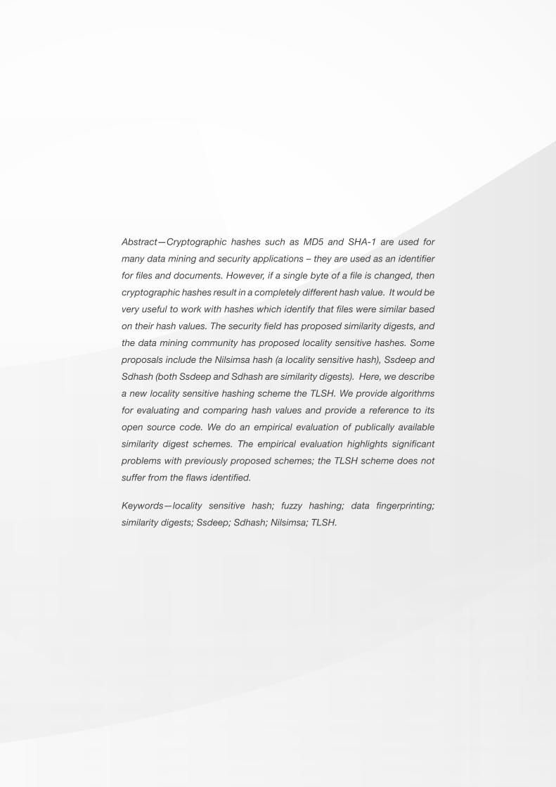
Abstract—Cryptographic hashes such as MD5 and SHA-1 are used for

many data mining and security applications – they are used as an identifier

for files and documents. However, if a single byte of a file is changed, then

cryptographic hashes result in a completely different hash value. It would be

very useful to work with hashes which identify that files were similar based

on their hash values. The security field has proposed similarity digests, and

the data mining community has proposed locality sensitive hashes. Some

proposals include the Nilsimsa hash (a locality sensitive hash), Ssdeep and

Sdhash (both Ssdeep and Sdhash are similarity digests). Here, we describe

a new locality sensitive hashing scheme the TLSH. We provide algorithms

for evaluating and comparing hash values and provide a reference to its

open source code. We do an empirical evaluation of publically available

similarity digest schemes. The empirical evaluation highlights significant

problems with previously proposed schemes; the TLSH scheme does not

suffer from the flaws identified.

Keywords—locality sensitive hash; fuzzy hashing; data fingerprinting;

similarity digests; Ssdeep; Sdhash; Nilsimsa; TLSH.

There are many problems in data mining where identifying near duplicates and similar files is useful.

This is especially true in the area of computer security where it is required to identify malware samples

with similar binary file structure, identify variants of spam email, etc. In some of these problems,

files or information is modified by accident, for example file corruption. In many applications, the

file is deliberately changed by an adversary. For example, in spam outbreaks, spammers will go to

significant effort to make sure that each spam email is unique - to avoid being matched to other spam

emails by the use of cryptographic hash functions.

Similarity digests [2, 3, 5] are an approach to solving these problems. Similarity digests attempt to

solve a nearest neighbour problem using a digest that is superficially similar to a cryptographic hash.

Approaches to this include schemes based on feature extraction [5], Locality Sensitive Hashing (LSH)

schemes [2, 10] and Context Triggered Piecewise Hashing (CTPH) schemes [3]. All these similarity

digest schemes have the property that a small change to the file being hashed results in a small

change to the hash. In this paper, we restrict the schemes we consider to those where the digest can

be encoded as a digest and stored in a central repository. The bit sampling approaches [2, 10] are

amenable to the creation of digests. For example, the random projection methods that approximate

the cosine distance between two feature vectors [7] are less amenable to the creation of digests. For

the methods which allow the creation of digests, the similarity between two files can be measured by

comparing the digests of the documents under consideration.

These schemes have been released as open source code: Ssdeep [3], Sdhash [5] and Nilsimsa [2,

10]. In the area of malware analysis, the de facto standard is the Ssdeep hash [8]. For example, NIST

supports Ssdeep [11] and Ssdeep is currently the only similarity digest supported by Virus-Total [13].

The Ssdeep scheme [3, 1] is a CTPH which segments the file, evaluates a 6 bit hash value for each

segment. Ssdeep calculates the edit distance between digests as the similarity measure. Sdhash [5, 6]

creates a similarity digest by identifying features with low empirical probability, hashing these features

into a bloom filter, and encoding the bloom filter as the output digest. Sdhash uses a similarity score

by calculating a normalized entropy measure between the two digests. The Sdhash scheme is close in

spirit to a random projection method of LSH schemes where the distance between two feature vectors

is the cosine distance between the feature vectors. The Nilsimsa scheme [2, 10] is a bit sampling LSH

which uses the hamming distance between the digests as the similarity measure.

Previously, limitations of Ssdeep for practical applications have been raised [1, 6]. Roussev concludes

that Sdhash consistently outperforms Ssdeep for the experiments performed [6].

This paper is organized as follows. Sections 2 and 3 give details of the TLSH scheme, including details

on construction of TLSH digests and scoring the distance between two digests. Section 4 gives an

empirical comparison of the TLSH scheme with the Ssdeep and Sdhash schemes. This evaluation

confirms the limitations which were raised in [1, 6], and identifies limitations of the Sdhash method

which have not been previously identified.

5 | TLSH - A Locality Sensitive Hash

Construction of the TLSH DIGESTIn this section, we describe how to construct a TLSH value from a byte string. The various parameters

and choices that were made are justified in Section 2(F). Source code which implements the algorithms

described here has been released as open source code [12].

We consider a byte string of length len:

Byte[0], Byte[1], Byte[2] … Byte[len-1]

The TLSH digest of the byte string is evaluated as the following steps

1. Process the byte string using a sliding window of size 5 to populate an array of bucket counts

2. Calculate the quartile points, q1, q2 and q3

3. Construct the digest header values

4. Construct the digest body by processing the bucket array

Steps 1, 2 and 4 combine to use a modified bit sampling method; instead of bit sampling these steps

are sampling pairs of bits. The sampling process is done to a finite precision so as to have a fixed length

digest. Step 3 constructs innovative features based on the approach used to get a fixed length digest.

Step 1. Process the byte string with a sliding window

The byte string is processed using a sliding window of size 5 to populate an array of bucket counts using

the following process:initialize the array bucket to 0

For ew = 4 to len-1 {

// sw is the start of the window

sw = ew - 4

For tri = 1 to 6 {

(c1,c2,c3)=Triplet(tri,Byte[sw..ew])

bi = b_mapping(c1, c2, c3)

bucket[ bi ] ++

}

}


Step 2. Calculate the quartile points

After step 1 has been performed we have an array of bucket counts. We calculate the quartiles of this

array such that:

75% of the bucket counts are >= q1



Step 3. Construct the digest header

The first 3 bytes of the hash are a header. The first byte is a checksum (modulo 256) of the byte string. The

second byte is a representation of the logarithm of the byte string length (modulo 256). The third byte is

constructed out of two 16 bit quantities derived from the quartiles: q1, q2 and q3:

q1_ratio = (q1*100/q3) MOD 16

q2_ratio = (q2*100/q3) MOD 16

Step 4. Construct the digest body

1. The remainder of the digest is constructed using the bucket array using the following procedure:

For bi = 0 to 127 {

if bucket[bi] <= q1 Emit(00)

else if bucket[bi] <= q2 Emit(01)

else if bucket[bi] <= q3 Emit(10)

else Emit(11)

}

Putting the digest together

The final TLSH digest constructed from the Byte string is the concatenation of:

• the hexadecimal representation of the digest header values from step 3, and

• the hexadecimal representation of the binary string from step 4.

Choices in the Construction Algorithm

A number of choices have been made in the algorithm used to construct a digest from a byte string. We

first list the choices, and offer an explanation for each choice below:

• A sliding window of size 5.

• We choose to extract triplets from the sliding window, and we selected 6 of the possible 10 triplets.


• The use of the Pearson hash as the bucket_mapping function.

• The use of quartiles instead of average or median.

• The use of a checksum and a length factor in the header.

• The form of the q_ratio parameters.

We selected a window size of 5 and to extract triplets from the sliding window because it had previously

been used in the Nilsimsa hash, and it had proved effective.

We selected 6 triplets of the 10 possible triplets for the following reason. There are 10 possible triplets of

bytes from a window of 5 bytes (A, B, C, D, E). The possible triplets are:

1. A B C

2. A B D

3. A B E

4. A C D

5. A C E

6. A D E

7. B C D

8. B C E

9. B D E

10. C D E

We excluded triplets 7 to 10 because they result in duplicated counting of triplets; each triplet from 7 to

10 will be processed in a subsequent iteration of moving the sliding window.

Implementation details: the source code that has been open sourced reverses each window of characters

before the 6 triplets are extracted and had the Pearson hash applied.

We selected the Pearson hash [4] as the bucket mapping function because it has a long history, and is

well respected.

We selected the quartile points rather than the average used by the Nilsimsa hash for a similar purpose to

make the scheme work well on binary data such as binary files and on images.

We selected a 1 byte check sum for false positive avoidance. Sometimes very similar long files (for

example, with only one byte difference) can get collisions and near collisions using LSH techniques. In

the open source software [12], this option is configurable.

We selected a 1 byte length description so that we can identify strings w hich have similar characteristics,

but are very different in size. In the open source software [12], this option is configurable.

The q_ratio parameters were determined through experimentation, and found to be useful.


Scoring the Distance Between two TLSH DigestsThe Ssdeep [3] and Sdhash [5] schemes provide a similarity score between two digests which ranges

from 0 to 100, where 0 is a mismatch and 100 is a perfect match (or a near perfect match). The results in

Section 4 highlight problems with the approach; and therefore the TLSH scheme uses a distance score.

The TLSH scheme scores the distance between two digests - a distance score of 0 represents that

the files are identical (or nearly identical) and scores above that represent greater distance between the

documents. A higher score should represent that there are more differences between the documents.

In this section, we describe how to score the distance between two TLSH digests. Source code which

implements this functionality is included in the open source code [12].

We define the mod_diff(X, Y, R) which is the minimum number of steps between X and Y on a circular

queue of size R:

mod_diff(X,Y,R) = MIN((X-Y) mod R, (Y-X) mod R)

For example, the mod_diff(15, 3, 16) = 4 because it requires 4 steps to go from position 15 to position 3

on a circular queue of size 16. The steps are:

15 → 0 → 1 → 2 → 3

We now calculate the distance score between two digests, tX and tY. Each of these digests is a hexadecimal

string, and we can extract the checksum, the lvalue, the q1ratio, the q2ratio from the first 6 hexadecimal

digits. The distance score between the tX and tY digests is defined as the sum of the distance of the

headers (as given by the distance_headers function below) and the distance of the digest bodies (as

given by the distance_bodies function below).


Function distance_headers(tX, tY)

int diff=0

ldiff = mod_diff(tX.lvalue, tY.lvalue, 256);

If ldiff <= 1

diff = diff + ldiff

else

diff = diff + ldiff * 12;

q1diff = mod_diff(tX.q1ratio, tY.q1ratio, 16);

If q1diff <= 1

diff = diff + q1diff

else

diff = diff + (q1diff-1) * 12;

q2diff = mod_diff(tX.q2ratio, tY.q2ratio, 16);

If q2diff <= 1

diff = diff + q2diff

else

diff = diff + (q2diff-1) * 12;

If tX.checksum <> tY.checksum

diff = diff + 1

return(diff)

Function distance_bodies(tX, tY)

int diff=0

For I = 1 to 64 {

x1 = tX.hex[i+5] / 4

x2 = tX.hex[i+5] % 4

y1 = tY.hex[i+5] / 4

y2 = tY.hex[i+5] % 4

d1 = abs(x1 – y1)

d2 = abs(x2 – y2)

if (d1 == 3)

diff = diff + 6

else

diff = diff + d1

if (d2 == 3)

diff = diff + 6

else

diff = diff + d2

}

return(diff)

This distance calculated by the distance_bodies(tX, tY) function is very similar to the methods used by

previous LSH methods that used a bit sampling method [10, 14]. The function calculates an approximation

to the hamming distance between two digest bodies. The difference between the method in the distance_

bodies()and using the hamming distance is the parameter 6 for the occasions when a bucket count

in the tX and tY are at the extreme points – that is for one of the digests the bucket count was in the top

quartile, and the other digest was in the bottom quartile.


Without loss of generality, consider the situation of x1=0 and y1=3. We derive the parameter 6 by

considering the binomial situation when p=.25 and n=3. The probability of getting an event is

Prob(k=3 | n=3; p=0.25) =(nk) p

k (1 - p)n-k

=0.0156

As noted in [2], the scoring of the hamming distance is equivalent to the negative logarithm to base two

of the probability of the events.

-log2(Prob(k=3 | n=3; p=0.25)) = 6

And hence the parameter in the distance_bodies() function for the situation is 6.

The distance calculated by the distance_headers() function also has a parameter. This time the range

of the binomial trials implied by the mod_diff() function is 16 for the qratios and 256 for the length. It is

not clear which distribution these parameters will follow – it will depend on the security application under

consideration. We considered two approaches for deciding the parameters to use in the distance_

header() function. The first approach was to extend the binomial argument used above to the case of

n=15 and p=1/16. This leads to a multiplier parameter of 3. The second approach was to plot the relative

occurrence of similar files having different qratios and lvalues. Inspecting the plots resulted in us selecting

a multiplier parameter of 12. Ideally, the multiplier parameter should be selected based on trials for the

data under consideration. For example executable files, image files, text files and source code have a

different distribution for the qratios and the lvalues. Based on the results in the next section, a choice of

12 for the multiplier parameter is fairly robust. We also note that the open source software [12] allows the

user to select options such as turning off any penalty for different lvalues.

The use of the checksum in the distance_headers() function was to make sure that digests from near

collisions have a distance score greater than 0.

The computation of this score can be significantly sped up by the use of pre-calculated tables, which is

implemented in the software [12].


ResultsThe TLSH scheme described has been implemented and source code has been made available online

[12]. Here we present some comparisons with Ssdeep [3], Sdhash [5] and Nilsimsa [10].

ROC Analysis

We collected a set of files that we knew were distinct: 109 binary malware files from different malware

families, 290 randomly constructed HTML fragments, 100 pieces of random text selected from the Unix

dictionary (with no overlap) and 79 distinct text files about different topics.

We collected a set of files where we knew that the files are similar. This set included 20 binary files from

the TROJ_DROPPER malware family, 20 binary files from the TROJ_ZLOB malware family, 20 binary files

from the WORM_SOBER malware family. We took each of the 79 distinct text files and mutated it into 14

variations for a total of 15 similar files. Five of the 14 variations had a word selected and globally replaced

by another random word selected from the text files. Three variations were created by using the Unix fmt

command changing the formatting of the text file to have a width of 40, 60 and 80 characters. Five further

variations were created by reformatting the file, and then globally replacing a random word with another

random word selected from the text files. One of the 14 variations was constructed by using the Unix “sort

--random-sort” to randomly sort the lines of the file.

The gold standard for this data set was a total of 8766 similar file comparisons and a total of 55822

different file comparisons. Ssdeep, Sdhash, Nilsimsa and TLSH were used to determine the similarity

and distance scores for the respective methods. Tables 1 and 2 give a range of thresholds and the false

positive rate and detection rate for each of the schemes.

The size of the data sets is relatively modest because it was important to check many of the pairs of files

by hand; to ensure that errors had not crept into the analysis.


Sdhash Ssdeep

Score FP rate Detect rate Score FP rate Detect rate

> 0 0.04711% 37.1% > 0 0.09966% 31.2%

> 5 0.02718% 36.6% > 5 0.09785% 31.2%

> 10 0.02174% 36.1% > 10 0.09603% 31.2%

> 20 0.01812% 35.4% > 20 0.09422% 31.2%

> 30 0.01268% 34.4% > 30 0.05617% 30.9%

> 40 0.00544% 32.7% > 40 0.01812% 29.3%

> 50 0.00362% 29.7% > 50 0.00362% 27.3%

> 60 0.00362% 26.0% > 60 0.00362% 25.9%

> 70 0.00181% 18.8% > 70 0.00181% 23.1%

> 80 0.00181% 12.4% > 80 0.00000% 16.2%

> 90 0.00181% 4.6% > 90 0.00000% 8.8%

> 99 0.00000% 1.0% > 99 0.00000% 3.5%

Table 1. False positive and detection rates for Sdhash and Ssdeep

TLSH Nilsimsa

Score FP rate Detect rate Score FP rate Detect rate

< 300 79.30% 98.8% > 120 99.86% 100.0%

< 250 69.06% 98.8% > 130 99.20% 100.0%

< 200 50.10% 98.8% > 140 98.11% 100.0%

< 150 24.33% 98.1% > 150 96.98% 100.0%

< 100 6.43% 94.5% > 160 94.26% 100.0%

< 90 4.49% 92.3% > 170 89.52% 100.0%

< 80 2.93% 89.0% > 180 81.38% 100.0%

< 70 1.84% 83.6% > 190 69.69% 99.7%

< 60 1.09% 76.0% > 200 54.45% 98.8%

< 50 0.52% 65.3% > 210 36.73% 96.4%

< 40 0.07% 49.6% > 220 18.29% 91.9%

< 30 0.00181% 32.2% > 230 5.52% 72.0%

< 20 0.00181% 17.3% > 240 1.26% 35.2%

< 10 0.00181% 6.4% > 250 0.49% 9.5%

Table 2. False positive and detection rates for tlsh and the Nilsimsa hash


We note the following from the tables:

• The schemes have different scoring ranges. TLSH distance scores go up to 300 (and can potentially

go up to over 1000). Sdhash and Ssdeep similarity scores are restricted to the range 0-100.

• The Nilsimsa hash typically gives scores in the range 128-256 – and rarely goes below 128. A Nilsimsa

score of 128 can be interpreted as meaning the files are completely different, while a score of 256

means the files are very similar.

• The Sdhash and Ssdeep schemes have very low false positive rates for all sensible thresholds, but

have a significantly lower range for their detection rate.

• The TLSH scheme has very low false positive detection capabilities at thresholds <= 30 and very high

detection rates for thresholds closer to 100. Of the four schemes, it is the only scheme which allows

for the user to select a threshold which enables tradeoffs to be made between false positive rates and

detection rates.

• The Nilsimsa scheme has very strong capabilities for detecting similar files, but suffers from significantly

higher false positive rates. We note that the results of the Nilsimsa scheme are strictly worse than the

TLSH scheme – so we drop the Nilsimsa scheme from further consideration.

We took the false positive and true positive rates for three of the schemes and created a ROC curve (for

clarity we have removed the Nilsimsa scheme since it is not a competitive scheme). Fig. 1 shows the ROC

curve where the scoring threshold was systematically varied to determine whether two files were a match

or not.

The ROC curve highlights a deficiency in the Sdhash and Ssdeep schemes. Limiting the scoring to 0-100

has resulted in schemes where there is no available threshold for many useful cases.

Figure 1. ROC Curve

1

.5

0

0 .5 1

TLSH

Sdhash

Ssdeep


For the Sdhash and Ssdeep schemes, this results in a ROC curve which abruptly changes in nature once

the threshold hits the score of 1. It is not a sensible use of these schemes to use a threshold of 0 – since

that is equivalent to asserting that all files are similar. From Table 1, we see that at a threshold of 1, Sdhash

has a false positive rate of 0.047% and a detection rate of 37.1%. At a threshold of 0, Sdhash has a false

positive rate of 100% and a detection rate of 100%. There are no thresholds available between these

extremes. We have drawn in this point on the ROC diagram so that we can calculate the ROC area.

The ROC area for each of the methods is shown in Table 3. We list the areas under the curves as a

standard part of a ROC analysis, while noting that the areas for the Sdhash and Ssdeep schemes were

dominated by the limitation on thresholds noted above.

TLSH Sdhash Ssdeep

Area under ROC curve

0.9775 0.6855 0.6555

Table 3. Area under ROC curve

The value in doing the ROC analysis was twofold:

1. It established that the various choices about the algorithm and parameters made in Sections 2 and 3

created a robust scheme.

2. It identified that using a scoring range of 0-100 created limitations for the Sdhash and Ssdeep

schemes.

Systematically Changing a File

We started with the first 500 lines of Pride and Prejudice (pg1342.txt from [9]). We created 500 versions of

this text, each one more `different` from the original text than the previous.

100

50

0

0 100 200

TLSH

Sdhash

Ssdeep

Figure 2. The scores on mutations of the first 500 lines of Pride and Prejudice.


The changes we introduced were random, and consisted of performing one of the following changes:

1. inserting a new word,

2. deleting an existing word,

3. swapping two words,

4. substituting a word for another word,

5. replacing 10 occurrences of a character for another character, or

6. deleting 10 occurrences of a character.

The scores comparing the original text with the files generated by this process for Ssdeep, Sdhash and

TLSH are shown below in Fig. 2.

We then applied the same approach to the entire text of Pride and Prejudice (13426 lines containing

704,146 bytes). We again iteratively applied changes. Due to the size of the book, at each iteration we

would do one of the following transactions:

A. apply 40 of the changes (1-6) described above,

B. swap two sections containing 5-25 lines, or

C. delete 5-25 lines.

The scores comparing the original text with the files generated by this process for Ssdeep, Sdhash and

TLSH are shown below in Fig. 3.

Figure 3. The scores on mutations of entire text of Pride and Prejudice.

100

50

0

0 100 200

TLSH

Sdhash

Ssdeep


In both Fig. 2 and Fig. 3, the Ssdeep and Sdhash similarity scores go down from 100 to 0, while the distance

score for TLSH grows. In both graphs, well after the Ssdeep and Sdhash methods have scored the files

as being distinct (a score of 0), the TLSH method is giving distance scores which can be interpreted as

saying the files are `similar` (in the range of 10 to 40).

Alarmingly for the Ssdeep method, in Fig. 3, the Ssdeep score immediately goes to zero after the 2nd

iteration of changes to the text. At this point the Unix diff command can determine that the files are very

similar – only 153 changes have occurred and the first change does not occur until line 44 out of 13426

lines.

A visual inspection of the files agrees with the TLSH scores. After 150 iterations of the process, where

both Sdhash and Ssdeep have failed to identify the files as being similar, a human reader can still say

with confidence that the text is the start of Pride and Prejudice. The first paragraph of the 150th iteration

of this process is shown in Fig. 4.

PRIDE AND PREJUDICEBy Jane AustenChapter 1It is a truth universally aiknowledged, younarenangreatndealntoonapt,nyoun-know, a single man in possession of a good fortune, must be in want of a wife.

Figure 4. The first paragraph of the 150th iteration of the mutation process.

Performance

We performed a comparison of the speed of the TLSH code. Table 4 below shows the TLSH performance

on Ubuntu machine (Intel Pentium 4 CPU 3.40 GHz, 4G RAM) compared to MD5, SHA-1 and Ssdeep.

The input data length is 4096 bytes, and the times were averaged over 10,000 computations of the hash.

MethodAverage time (microsecond)

TLSH 286

MD5 38

SHA1 53

Ssdeep 265

Table 4. Average speed for calculating the digests

The speed of TLSH is about the same as Ssdeep.


ConclusionThis paper has described the TLSH approach based on Locality Sensitive Hashing for implementing

similarity digests. The approach described here has been released as open source code [12].

The ROC analysis highlighted a significant problem with the range of values which the Sdhash and Ssdeep

similarity score can take. Restricting this to a range of 0-100 limits the usefulness of the schemes.

The TLSH scheme described has outperformed available digest methods for identifying similar documents,

especially for applications where missed detections are of concern and false alarms are acceptable. The

TLSH method shows distinct advantages in the nature of its ROC curve, and therefore has a wider range

of computer security applications. The empirical evaluation highlights significant problems with previously

proposed schemes.


References

1. F. Breitinger, “Sicherheitsaspekte von fuzzy-hashing”. Master’s thesis. Hochschule Darmstadt, 2011.

2. E. Damianil, S. De Capitani di Vimercati1, S. Paraboschi2, and P. Samarati, “An Open Digest-based Technique for Spam Detection” in Proc. of the 2004 International Workshop on Security in Parallel and Distributed Systems, San Francisco, 2004.

3. J. Kornblum, “Identifying Almost Identical Files Using Context Triggered Piecewise Hashing” in Proc. of the 6th Annual DFRWS, 2006, S91-S97. Elsevier.

4. P.K. Pearson, “Fast Hashing of Variable-Length Text Strings,” Communications of the ACM. 33, 1990, 677-680.

5. V. Roussev, “Data Fingerprinting with Similarity Digests” in Research Advances in Digital Forensics VI. 207-226. Chow, K.; Shenoi, S. (eds), 2010, Springer.

6. V. Roussev, “An Evaluation of Forensics Similarity Hashes” in Proc. of the 11th Annual DFRWS, S34-S41, 2011, Elsevier.

7. R. Shinde, A. Goel, P. Gupta and D. Dutta, “Similarity search and locality sensitive hashing using ternary content addressable memories” in Proc of the 2010 International Conference on Management of Data, June 06-10, 2010, Indianapolis.

8. Cisco Blog:

9. http://blogs.cisco.com/security/malware_validation_techniques/

10. Gutenberg Project: http://www.gutenberg.org/

11. Nilsimsa: http://ixazon.dynip.com/~cmeclax/nilsimsa.html

12. NIST: http://www.nsrl.nist.gov/ssdeep.htm

13. TLSH: https://github.com/trendmicro/tlsh/

14. Virus Total: http://www.virustotal.org/

15. Wikipedia LSH: http://en.wikipedia.org/wiki/Locality-sensitive_hashing

©2017 by Trend Micro, Incorporated. All rights reserved. Trend Micro and the Trend Micro

t-ball logo are trademarks or registered trademarks of Trend Micro, Incorporated. All other

product or company names may be trademarks or registered trademarks of their owners.

TREND MICROTM

Trend Micro Incorporated, a global cloud security leader, creates a world safe for exchanging digital information with its Internet content security and

threat management solutions for businesses and consumers. A pioneer in server security with over 20 years experience, we deliver top-ranked client,

server, and cloud-based security that fits our customers’ and partners’ needs; stops new threats faster; and protects data in physical, virtualized, and

cloud environments. Powered by the Trend Micro™ Smart Protection Network™ infrastructure, our industry-leading cloud-computing security technology,

products and services stop threats where they emerge, on the Internet, and are supported by 1,000+ threat intelligence experts around the globe.

For additional information, visit www.trendmicro.com.

Documents

TLSH - A Locality Sensitive Hash - Trend Micro Internet ... · Nothing contained herein should be relied on or acted upon without the benefit of ... emails by the use of ... TLSH