WIND TURBINE TLP DESIGN PROJECT

Prepared By: Group 7: Patrick Burnett, Dale Cressman, Oguzhan Kirikbas, Daniel Place, Jin Zhang

Graduate Students, Department of Naval Architecture and Marine Engineering The University of Michigan

Prepared For:

Matthew Collette Professor, Department of Naval Architecture and Marine Engineering

The University of Michigan

2

Table of Contents List of Tables .................................................................................................................................. 3 List of Figures ................................................................................................................................. 3 1.0 – Introduction ............................................................................................................................ 4 2.0 – Problem Statement ................................................................................................................. 5

2.1 - Design Methodology .......................................................................................................... 5

3.0 – Particle Swarm Optimization ................................................................................................. 7 3.1 – Background ........................................................................................................................ 7 3.2 - Implementation ................................................................................................................... 8

4.0 – Hydrostatics ......................................................................................................................... 10 5.0 – Forces and Loads ................................................................................................................. 11

5.1 – Turbine Supplied Loads ................................................................................................... 11 5.2 – Wind Induced Loads ........................................................................................................ 11 5.3 – Current Induced Loads ..................................................................................................... 12

6.0 – Stresses ................................................................................................................................. 13

6.1 - Bending ............................................................................................................................. 13 6.2 - Hoop ................................................................................................................................. 14 6.3 - Axial ................................................................................................................................. 14

6.4 - A-36 Steel and combined stresses .................................................................................... 14 6.5 – Tension Leg Support ........................................................................................................ 14

7.0 – Seakeeping ........................................................................................................................... 15 7.1 - Heave Natural Period........................................................................................................ 15 7.2 - Surge/Sway Natural Period .............................................................................................. 16 7.3 - Setdown ............................................................................................................................ 16 7.4 – Pitch Angle Calculations.................................................................................................. 17

8.0 – Cost Calculation ................................................................................................................... 18 9.0 - Design Overview .................................................................................................................. 19 Works Cited .................................................................................................................................. 21 Appendix A – Particle Swarm Optimization Code ....................................................................... 22 Appendix B – Hydrostatics Code ................................................................................................. 27 Appendix C – Load Calculations .................................................................................................. 30

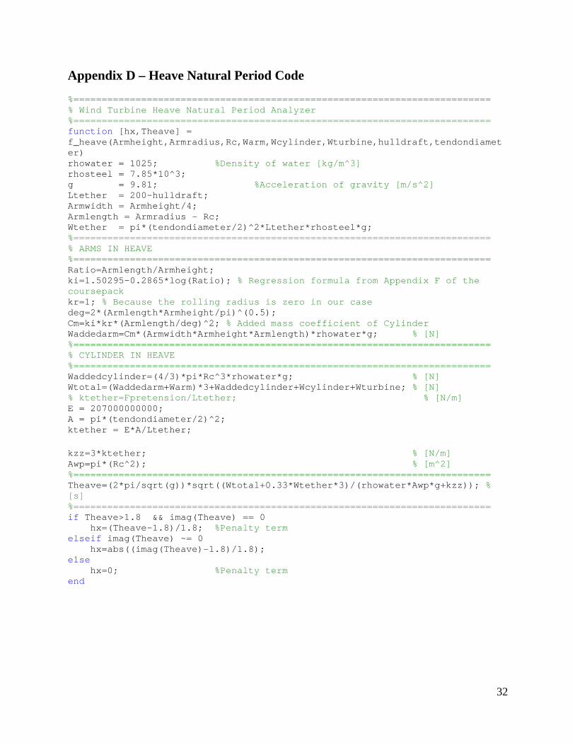
Appendix D – Heave Natural Period Code ................................................................................... 32 Appendix E – Pitch Calculation Code .......................................................................................... 33 Appendix F – Setdown Condition Analyzer ................................................................................. 34 Appendix G – Surge Calculation Code ......................................................................................... 36 Appendix H – Cost Calculation Code ........................................................................................... 37

3

List of Tables

Table 1- NREL 5MW Turbine Properties [2] ................................................................................. 5 Table 2 - Definition of the Design Variables .................................................................................. 6 Table 3 - Model of Testing & Design Constraints .......................................................................... 6 Table 4 - Final Design Dimensions .............................................................................................. 19 Table 5 - Final Design Properties ................................................................................................. 20

List of Figures

Figure 1 - Wind Resources in the United States [1] ....................................................................... 4 Figure 2 - The Design Process of the Floating TLP Platform Structure ......................................... 7 Figure 3 - Power Curve for NREL 5 MW Turbine ....................................................................... 11 Figure 4 - Drag Coefficients ......................................................................................................... 13 Figure 5 - Comparison of the System Natural Periods ................................................................. 15 Figure 6 - Free Body Diagram of Setdown ................................................................................... 17 Figure 7 - Free Body Diagram of Pitched TLP............................................................................. 18 Figure 8 – Design Drawing - Overview ........................................................................................ 39 Figure 9 – Design Drawing – Front View .................................................................................... 40 Figure 10 – Design Drawing – Base Dimensions ......................................................................... 41 Figure 11 – Design Drawing – Side View .................................................................................... 42

4

1.0 – Introduction Renewable wind energy is one of the most promising sources of clean power in the foreseeable future. As technology progresses to improve the feasibility of the wind energy systems, additional locations, such as offshore platforms become a reality to aid in the progress of electricity generation. As suitable marine wind farm locations have been explored the distance offshore has steadily increased, from the shallow waters of Denmark to depths of hundreds of meters. The original wind turbine platforms were in approximately 30 meters of water, but have steadily increased to around 80 meters depth. The feasibility of the successful areas for wind farms was severely limited to these water depths, as the platforms were required to be bottom fixed. [1] Mono-pile platforms, consisting of a single support tower were anchored to the seabed for the shallow water applications, while applications from 20-80 meters used a tripod design, also fixed to the seabed. In order to exploit better wind farm locations that are further offshore, and thus in deeper water, new technologies, often applied from the offshore oil industry, must be developed. One of these technologies is the Tension Leg Platform (TLP), allowing for significantly greater water depths, proposed up to 900 meters in depth. In the United States, much of the developable areas for wind farms are farther offshore than depths of 80 meters, as shown in Figure 1. This leads to the need to utilize tension leg platforms to successfully harness the winds power.

Figure 1 - Wind Resources in the United States [1]

5

2.0 – Problem Statement The ability to utilize the areas of the United States that are suitable for wind energy development requires a TLP is to be designed to support a 5 MW National Renewable Energy Lab (NREL) Offshore Wind Turbine with a concrete gravity base for use in 200 meters of water. 100 turbines are to make up the wind farm. Designing a TLP for use in 200 meters of depth requires overcoming significant design challenges not faced in the design of a land based or bottom fixed system. Details of the NREL 5 MW turbine are outlined in Table 1.

Table 1- NREL 5MW Turbine Properties [2]

In order to ensure the safety and operation of the installed wind turbine, the platforms are limited to natural heave periods of less than 1.8 seconds, surge/sway periods of greater than 70 seconds, tendon tension greater than zero, a maximum set-down of less than 1.2 meters in storm conditions of 120 knots and 3 knots of current, and a 3 degree pitch limitation in storm survival conditions. The objective was to produce a platform capable of meeting these criteria with the minimum total cost.

2.1 - Design Methodology

The objective of the design process was to minimize the costs of the support structure for the NREL 5 MW Wind Turbine. The design team started with real data from the given wind turbine and the customer requirements as outlined above. Choosing variables to describe the structure geometrically, a PSO was utilized to explore the design space. The design variables describe the geometry of the supporting structure. Based on an initial feasible design the design variables were reduced to: hull draft, hull diameter, arm length, arm height, hull radius, arm thickness, tendon diameter and ballast height. The design variables and their descriptions are indicated in Table 2.

6

Design Variables Definition hull draft The distance from the bottom of the hull to the free surface hull radius The distance from the center to the outer surface of the hull arm length The horizontal dimension of the arm from the hull arm height The vertical dimension of the arm hull thickness The thickness of the steel A-36 for hull arm thickness The thickness of the steel A-36 for arm tendon diameter The diameter of the tendon ballast height The vertical dimension of the ballast from the hull bottom

Table 2 - Definition of the Design Variables The PSO checked the fitness based on the feasability of the three catagories shown in Table 3. Those catagories were used to analyze the structure and apply penalties to the objective cost function if the point designs violated any constraints. The objective of the design process was to reduce the cost of the structure. The cost calculation was used as an evaluation function to obtain the best group of design variables. The overall design process is described in Figure 2.

Catagory Analysis Hydrodynamics Turbine Heave Natural Period Analyzer

Pitch Angle Analyzer (Under 25 m/s wind speed) Setdown Condition Analyzer Surge Period Analyzer

Hydrostatics Buoyant Forces Calculation Structural Weight Calculation Tendon Force Calculation

Loads/ Stress Bending Loads Testing Wind Loads Testing Stress Testing

Table 3 - Model of Testing & Design Constraints

7

Figure 2 - The Design Process of the Floating TLP Platform Structure

3.0 – Particle Swarm Optimization

Complex design problems containing a multitude of design variables and constraints are virtually impossible to solve without the use of a rigorous optimization technique. Design problems containing one objective function are much more simple that multi-objective problems because a converged design can be obtained via optimization without having tradeoffs between conflicting objectives. Many different optimization techniques can be applied to single objective optimization problems but for a problem requiring strong global searching power, a particle swam optimizer (PSO) may be the best choice.

3.1 – Background

A PSO employed for a design problem initially generates a population of “individuals” (point designs) with random values for the independent variables governing the problem. These independent point designs’ variables are then given random “velocities” which changes each variable based on which initial random design was the “best” at satisfying the objective function (cheapest design, strongest design, fastest design, etc.). Theses individual design “particles” are then allowed to search around the design space with some degree of randomness, but at the same time, they are updated with information about which individual design is the best and whether their new “position” in the design space is better than the last. Specified coefficients determine how fast the individuals converge to the best design found and to what degree they ignore the current best solution and keep searching.

8

����� = ��� + ��� [1]

����� = ����� + ������ ������,� − ���� + ���� �����,� − ���� [2]

Equation 1 shows how the individuals’ positions (values) are updated with a velocity term. Equation 2 shows how the velocity is calculated, where w is an inertia term, c1 and c2 are individual and group learning rates, r1 and r2 are random numbers between zero and one, and Pbest and Gbest are current personal and current group best designs. The simplicity of the code made it a perfect option for applying to the problem of minimizing the cost of a wind turbine supporting TLP. The PSO allows the design variables to vary across the design space, however penalties must be imposed to prevent constraints from being violated and designs from going into the infeasible domain. Exterior penalty functions are useful because they allow the design space to remain intact while penalizing the optimizer for attempting to choose designs outside of the feasible domain. If a constraint “g” is violated, then equation 3 describes how the penalty term is generated. The penalized objective function then becomes equation 4, which allows the optimizer to realize which designs are the worst and best based on a value rk scaled by the sum of each constraint violations raised to the q power.

� � �� > 0, �ℎ�� �(�) = |� ��|, p=0 otherwise [3]

�(�) = �(�) + ���(�)� [4]

3.2 - Implementation

A PSO worked very well for optimizing the design of a TLP for a wind turbine because the single objective was to minimize cost and the constraints were quantifiable and easily determined based on the selected independent variables. The implementation of the raw PSO code was performed with Matlab and required the use of a “while” loop to continue running the PSO until the costs of all the individuals were less than one standard deviation. It was initially believed this might cause the PSO to converge to similar costs for different designs, however this was never the case. Occasionally, the PSO would get stuck converging on an infeasible design and would not be able to improve the design, in which case it was necessary to terminate the code and start the optimizer with a new random initial population. The nature of a PSO is to allow the design variables to vary with some degree of randomness, which allows a more global search of the design space. While this is a good technique for searching power, it can also allow individuals to have a combination of variables which do not make sense physically. Negative dimensions, steel thicknesses greater than member dimensions, imaginary numbers, and negative costs were the main issues which needed to be addressed. It was necessary to constrain the initial population to designs which made physical sense in order to give the PSO a baseline from which to search in the feasible domain. Initially the optimizer would converge on designs which had obtained negative costs which resulted from the code considering and favoring zero or negative dimensions. This issue was solved by not allowing the optimizer to chose a design with a negative cost as a personal or global best and penalizing the

9

objective function heavily (g(x) = 10 plus a normalized fraction of how negative the cost was). Designs with negative dimensions were penalized with g(x) = n*1 where n is the number of dimension violations. Penalty terms were normalized such that each term would cause a penalty relative to the severity of the constraint violation (Formula 5).

� �� =������� ����� − ��������� �������������� �����

[5]

Normalizing all the penalty terms to an order of 1-10 allowed none of the penalty terms to dominate the others. The exception was for negative cost, which was heavily penalized as discussed above. Dimension variable physically impossible, such as arm height exceeding the hull draft were penalized. If the PSO did allow variables to become negative, this typically resulted in formulas containing square roots to output imaginary numbers. Initially the PSO did not know how to handle these numbers and would either get stuck or output an imaginary cost. It was originally thought that the variables should be forced to remain in the feasible domain by changing their values positive if they became negative but this actually created additional problems and did not converge on any design. The final solution was to penalize a function not only if a constraint was violated, but also if an imaginary value was calculated. This allowed the PSO to have more freedom and searching power because these areas of the design space were still able to be searched for feasible solutions. Any imaginary or negative values were eliminated from the population within a few generations and the PSO never converged on any designs with negative or imaginary dimensions or cost. Conditions where the objective function received a penalty are listed below:

• Negative dimensions or cost • Imaginary variables or cost • Specified strength or dynamics requirements are not satisfied

• Hull radius is less than 5m diameter turbine column • Steel plate is less than 3 mm or greater than 50 mm

• Twice the arm plate thickness is greater than the arm width • Ballast height is greater than half the hull draft

Six subjective parameters required for the PSO were selected based on experience gained by running the code and interpreting the behavior of the PSO and its results. The inertial term dictates how fast a variable is allowed to change based on how much it changed during the previous iteration. This was the most influential parameter for obtaining good results from the PSO. Early on in the process, a value of w=0.5 was used. Different designs were converged upon each time the optimizer ran, creating the illusion there were many different best design choices. Increasing the inertia term to w=0.8 caused the optimizer to run at least three times longer but the same design was converged upon virtually every time.

The number of point designs which are being used in a PSO is called the population size. Increasing the population size allows more global searching power but also slows down the optimizer substantially. A population size of 50 individuals was used to debug the code, which only took ~20 seconds to run, but each time it ran the optimizer would converge on a design

10

different enough to warrant a greater search. A population of 200 individuals was used to produce the final design for this project and the difference in the designs between runs was small enough to be within construction error.

The group and personal learning rates scaled how much the global best design and the individual particles best design influenced how the variables changed with each iteration. The individual learning rate was set at c1=1.2 and the group learning rate was set at c2=1.5 forcing the optimizer to have more preference on the best design found by the group rather than an individual’s best design, while still allowing the individuals to search. Changing these values did not have a significant effect on the results.

The penalty function parameter rk has the same units as the objective function, in this case cost. It is scaled by the summation of all of the penalty terms and added to the cost function to form the penalized objective function. Initially a value of rk=$106 was chosen but it was obvious that the penalization was not sufficient because irrational designs were still being converged upon. Increasing the penalty parameter to rk =$109 was enough to force the PSO to virtually only converge on feasible designs. The penalty function also scaled each penalty term by g(x)r where typically r=2. This value not changed because increasing it would reduce the importance of any penalty terms less than one.

4.0 – Hydrostatics Primarily, the TLP must successfully support the weight of the entire wind turbine assembly, tower, and housing. Much of the actual design variable calculations that ensure the safety and feasibility of the design are computed from the hydrostatic calculations, ensuring the platform's ability to float. With the random input variables that the PSO code produced the volume for the hull and arms were calculated to produce a buoyant force according to the equation: �� = ∇ ∗ �� [6] Where: �� = ������� ����� ∇ = ������� !����� �� = ����� �� ���� ����� These dimensions were then used to compute the weight of the structure, including stiffeners, by taking the volume multiplied by the density of steel and a 1.4 allowance for the stiffeners. The total weight for the TLP platform was resolved by: "����� = "���� + "����� �� ���� + "����� + "�� �� + "������� [7] Where, Wrotor = 111000 kg, Wtower = 347000kg, and Wnacelle = 240000 kg in accordance with the National Renewable Energy Laboratory Technical Report NREL/TP-500-38060 [2]. Taking the calculated weight and subtracting it from the buoyant force gave the net resultant buoyant force, or the tendon pretension. Taking the tendon pretension and multiplying by the required factor of safety of 1.5, gave a result for the required concrete foundation weight for the platform. The

11

following penalty terms were used to ensure convergence on a feasible design: hull diameter larger than the tower diameter, positive hull draft, positive arm radius, positive hull and arm thicknesses, and positive tendon diameter are all normalized to provide individual penalty terms to the PSO program. 5.0 – Forces and Loads

5.1 – Turbine Supplied Loads

The TLP will experience different loading conditions which the structure must be able to handle. Two of these loads are directly due to the power generation function of the turbine. The generator and turbine produce forces and large moments as the blades spin and turn wind velocity into rotational motion. Figure 3 is the power curve for the NREL 5 MW turbine.

Figure 3 - Power Curve for NREL 5 MW Turbine

Figure 3 provided two values used in the following force calculations, RotTorq and RotThrust. The approximate maximum values for each, 4100 kNm and 900 kN occurring around 11.5 m/s, were used because they represented the worst case scenario. As wind velocity increases the turbine blades are designed to be pitch-regulated in order to prevent damage.

5.2 – Wind Induced Loads

The wind force was calculated using Equation 8. "� ����� = �#!�($�)�($��)�%� ∗ 1000

�

���

[8]

Where: K = units constant = 0.0000623 ts2/m4 V i = wind velocity at element center CS = Shape factor of element

12

CSH = Shielding factor Design criteria stipulated that the platform have 2m of freeboard so the wind was assumed to be acting on only 3 “elements.” The three elements were the circular platform which was being designed, the 90m tall tower of the wind turbine, and the generator located at the top of the turbine. For the generator forces it was assumed that all the forces acting on the blades and generator dimensions were accounted for in the RotThrust and RotTorq values. Equation 9 was used to determine the wind velocity at each of the element’s centroid heights. !�!� = (

&�'�)�� [9]

Where i represents the value for velocity or height at the element centroid and h represents the reference values. Two reference conditions were used; a storm condition of 61.733m/s at a height 10m above the water surface and a pitch check condition of 25 m/s at the same 10m height. The shape factor, CS, was .5 for both the tower and main hull cylinders. The shielding factor was assumed to be 1.

5.3 – Current Induced Loads

The current loads were calculated in a similar manner to wind loads. However, it was assumed the current was a constant 3 knots at all depths. With three legs each located 120° apart the design team had to determine which current loading scenario presented the worst case. If angle zero represents when the current is heading in a direction directly aligned with one of the platform legs than it was determined the worst case current occurred at angle 0 degrees. Equation 10 shows how the current force was calculated.

$����������� = � 1

2∗ $��

∗ �ℎ� ∗ !� ∗ %���

���

[10]

Where: CDi = Current drag coefficient A i = Normal area for element V i = Current velocity at element = 3 knots rho = density of saltwater

13

The drag coefficient changed depending on the shape of the area. Figure 4 was used to write a code which determined what the drag coefficient would be for the various dimensions which were input.

Figure 4 - Drag Coefficients

6.0 – Stresses

6.1 - Bending

The turbine, wind, and current forces all created moments which acted upon the bottom of the structure. In order to get the total moment acting on the structure a sum of each element force multiplied by its distance from the bottom of the structure was computed. The sum of the squares with RotTorq gave the largest total moment as shown in equation 11. (���� )����� = *�(+������ )������) + ,��(��-�

[11]

The bending stress could then be calculated with the known moment of inertia. The equations for both are given below.

14

.������� =)�� [12]

� =

�

�(, � − ,!�) [13]

6.2 - Hoop

The hoop stress was calculated just like a thin-walled pressure vessel. In this case the pressure is acting from the outside due to the hydrostatic water pressure. Equation 12 displays how the hoop stress was calculated; where P is the pressure from the water, D is the diameter of the cylinder, and t is the thickness of the cylinder. .���" =

�/2� [14]

6.3 - Axial

The final load which the design team used to test the structure was axial, or compressive, stress. This stress only acted upon the bottom of the structure and was the result of buoyancy. It was calculated using equation 15. .�#��� =

0,�/� [15]

6.4 - A-36 Steel and combined stresses

As part of the design requirements, the team was required to use ASTM A-36 Steel. A-36 is a standard carbon steel with yield strength of 250 MPa and elastic modulus of 207,000 MPa. The three main stresses (bending, hoop, and axial) all interact with each other at the bottom of the structure. In order to ensure that the A-36 steel did not yield under the stress, the Von Mises yield criterion was checked. The design team used a safety factor of 1.5 in the below Von Mises check. $�����

�

�.%≥ (.������� + .�#���)-(�.������� + .�#���� ∗ .���") + .���" [16]

6.5 – Tension Leg Support

The other part of the structure which the stresses were analyzed in were the leg supports. It was assumed that the legs acted as a cantilever beam of height “h” and width “b”. The stress would therefore be the same as the bending stress expressed in equation 12, however the moment of inertia changes to the following for a rectangular beam: � =

1

12�ℎ& [17]

15

Since the largest stress will occur at the bottom of the leg supports, using the parallel axis theorem, the moment of inertia was changed to: �'( ≈ 2

1

12�ℎ& + 2��(ℎ

21 ) [18]

For plate buckling we needed to calculate beta and use it to ensure the A-36 steel was strong enough. Equations 15 and 16 show how beta and the buckling stress were calculated. 2 =

�� 3 .)����+����� )� ����

[19]

.������� = 422 −125 ∗ .)���� [20]

7.0 – Seakeeping In order to avoid resonance with the wave exciting frequencies and vibration issues, the natural heave and surge/sway periods were important design considerations in the preliminary design stage of the TLP.

Figure 5 - Comparison of the System Natural Periods

7.1 - Heave Natural Period

As a design constraint, heave natural period has to be less than 1.8 seconds. The equation for heave natural period is presented in Equation 19. The tradeoffs that can be made for decreasing the heave natural period in order to operate the TLP out of the probable resonance range are decreasing total weight of the platform, increasing the waterplane area or increasing the stiffness of tethers. The calculated heave natural period for this design is T*,+,-., = 1.8 seconds.

16

T*,+,-., =

2π

6g∙ * 1 + A//�∆ + 0.33W0

ρgA12 + k// [19]

Where: g= Acceleration due to gravity. A// = Net added mass coefficient. W0 =Tether weight in air. ∆ =Dispacement. k// =Tether stiffness in heave. A// is calculated by using component-wise added mass formula: � w3 + w-3� = (1 + A//)∆ [20]

7.2 - Surge/Sway Natural Period

Similar to heave, surge/sway motions have to be considered in the preliminary design stage due to resonance related issues. Although satisfying the design constraint of 70 seconds is sufficient, surge/sway natural periods of the design should be as large as possible, preferably around 100 seconds. The equation for sway period is shown in Equation 21. It is possible to increase surge/sway natural period by decreasing the pretension of the tethers, increasing the total weight of the platform, or increasing the length of tethers. It can be easily seen that there is a tradeoff between surge/sway and heave natural period calculations. The final design has a 71.8 second surge/sway natural period.

T*,4567,/41-8 =2π

6g∙ *�1 + A9988�∆ + 0.23W0

P:/L [21]

Where: g= Acceleration due to gravity. A9988 = Net added mass coefficient. W0 =Tether weight in air. ∆ =Dispacement. P: = P; − 0.5 ∙ submerged weight of the tether� = Pretension in the middle The added mass correction coefficients Kr and Ki values are obtained from the regression curves.

7.3 - Setdown

A methodology that assumed a triangular geometry formed by a horizontally offset TLP due to current and wind loads was used in order to perform setdown calculations. This geometry was assumed to be independent from pitch calculations and take into account the elongation of the tendons due the total force increment. This methodology provided an accurate calculation of

17

setdown. The set down of the optimized design was 0.331 meters which easily satisfied the design constraint of 1.2 meters. A free body diagram of the setdown condition is presented below as Figure 6.

T 1T 2z

x

Fb u o y 2Fb u o y 1

S E A B O T T O M

m gm g

H

F h o riz o n ta l

L te th e rL te

ther + d

L

x

z

Q

Figure 6 - Free Body Diagram of Setdown

The stiffness coefficient of the tethers can be calculated by using Equation 22.

k0,;+,6 = � AE

L0,;+,6 [22]

Setdown is determined by the Equation 23 where “z” is the setdown in meters.

����F�������.

�� + (F������� + ρπR�zg)��kTether

� − (L� �� � − z)��(L� �� � − z)

∙ (F������� + ρπR�zg) − F�������.

= 0

[23]

7.4 – Pitch Angle Calculations The pitch motion was another aspect analyzed during the preliminary design stage. The design had a constraint of 1.5 degrees in 25m/s wind, and 3 degrees during storm survival. The methodology used for pitch calculations assumed that these calculations are dependent from the setdown case and all the loads are acting on a single point. Also, it was assumed that the structure was in steady state and the heel angle was zero at the beginning. During calculations

18

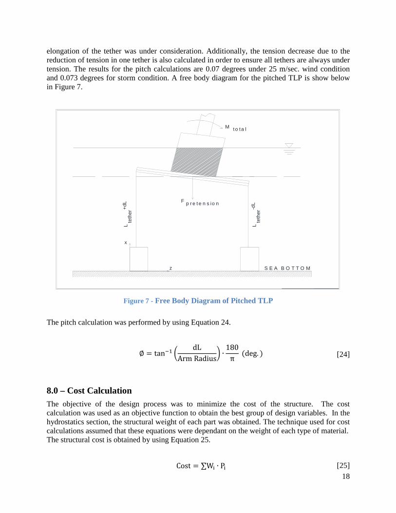
elongation of the tether was under consideration. Additionally, the tension decrease due to the reduction of tension in one tether is also calculated in order to ensure all tethers are always under tension. The results for the pitch calculations are 0.07 degrees under 25 m/sec. wind condition and 0.073 degrees for storm condition. A free body diagram for the pitched TLP is show below in Figure 7.

Lte

ther

+dL

S E A B O T T O Mz

x

Lte

ther

-dL F p r e t e n s io n

M to ta l

Figure 7 - Free Body Diagram of Pitched TLP

The pitch calculation was performed by using Equation 24.

∅ = tan<� 4 dL

Arm Radius5 ∙

180

π (deg. ) [24]

8.0 – Cost Calculation The objective of the design process was to minimize the cost of the structure. The cost calculation was used as an objective function to obtain the best group of design variables. In the hydrostatics section, the structural weight of each part was obtained. The technique used for cost calculations assumed that these equations were dependant on the weight of each type of material. The structural cost is obtained by using Equation 25.

Cost = ∑W3 ∙ P3 [25]

19

Where: W� = W=;,,>, the weight of the steel ASTM A-36 with 40% additional weight for structure W = W?@*?6,;,, the weight of the concrete used in the foundation and ballast W& = W;,*A@*, the weight of the tendon P� = P=;,,>, the unit price of steel ASTM A-36, 800 USD / metric ton including fabrication P = P?@*?6,;,, the unit price of concrete, 100 USD / metric ton including fabrication P� = P;,*A@*, the unit price of tendon, 8000 USD / metric ton

9.0 - Design Overview

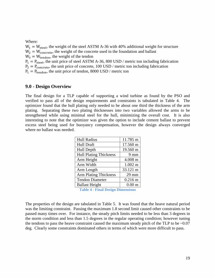
The final design for a TLP capable of supporting a wind turbine as found by the PSO and verified to pass all of the design requirements and constraints is tabulated in Table 4. The optimizer found that the hull plating only needed to be about one third the thickness of the arm plating. Separating these two plating thicknesses into two variables allowed the arms to be strengthened while using minimal steel for the hull, minimizing the overall cost. It is also interesting to note that the optimizer was given the option to include cement ballast to prevent excess steel being used for buoyancy compensation, however the design always converged where no ballast was needed.

Hull Radius 11.785 m Hull Draft 17.560 m Hull Depth 19.560 m Hull Plating Thickness 9 mm Arm Height 4.008 m Arm Width 1.002 m Arm Length 33.121 m Arm Plating Thickness 29 mm Tendon Diameter 0.216 m Ballast Height 0.00 m

Table 4 - Final Design Dimensions The properties of the design are tabulated in Table 5. It was found that the heave natural period was the limiting constraint. Passing the maximum 1.8 second limit caused other constraints to be passed many times over. For instance, the steady pitch limits needed to be less than 3 degrees in the storm condition and less than 1.5 degrees in the regular operating condition; however tuning the tendons to pass the heave constraint caused the maximum steady pitch of the TLP to be ~0.07 deg. Clearly some constraints dominated others in terms of which were more difficult to pass.

20

Total Weight 119.96 t Total Buoyancy 842.24 t Tendon Pretension 256.47 t Current Force 438.36 kN Foundation Weight 435.97 kN Storm Wind Force 81.81 kN Regular Wind Force 13.42 kN Storm Total Moment 106248.20 kNm Regular Total Moment 101957.51 kNm Heave Natural Period 1.80 s Surge Natural Period 71.80 s Storm Steady Pitch 0.07 deg Regular Steady Pitch 0.07 deg Set Down 0.33 m Stress, Axial 115.71 MPa Stress, Bending 22.48 MPa Stress, Combined 40668894217 MPa Stress, Hoop 231.41 MPa Stress, Leg 237.07 MPa

Table 5 - Final Design Properties

21

Works Cited

[1] Offshore Wind Energy. Environmental and Energy Study Institute. Oct. 2010. Web. 20 Mar.

2011. <http://www.eesi.org/files/offshore_wind_101310.pdf>.

[2] Jonkman, J., S. Butterfield, W. Musial, and G. Scott. Definition of a 5-MW Reference Wind

Turbine for Offshore System Development. National Renewable Energy Laboratory. Feb.

2009. Web. 17 Feb-25 Mar. 2011.

22

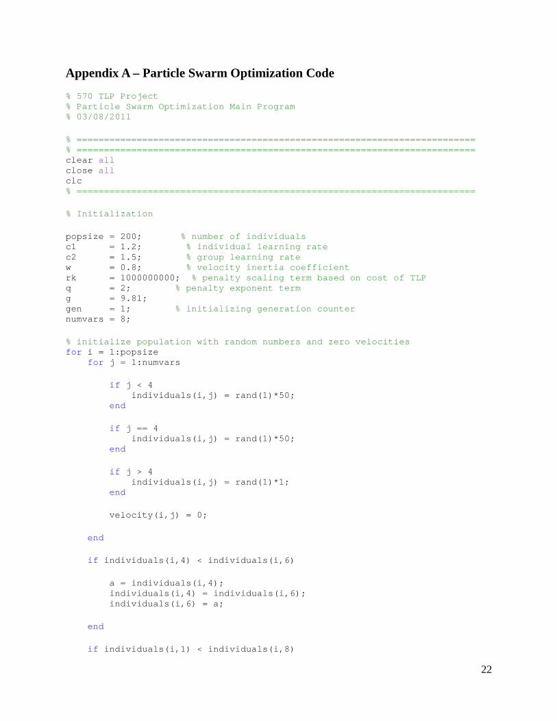
Appendix A – Particle Swarm Optimization Code

% 570 TLP Project % Particle Swarm Optimization Main Program % 03/08/2011 % ================================================= ======================== % ================================================= ======================== clear all close all clc % ================================================= ======================== % Initialization popsize = 200; % number of individuals c1 = 1.2; % individual learning rate c2 = 1.5; % group learning rate w = 0.8; % velocity inertia coefficient rk = 1000000000; % penalty scaling term based on cost of TLP q = 2; % penalty exponent term g = 9.81; gen = 1; % initializing generation counter numvars = 8; % initialize population with random numbers and zer o velocities for i = 1:popsize for j = 1:numvars if j < 4 individuals(i,j) = rand(1)*50; end if j == 4 individuals(i,j) = rand(1)*50; end if j > 4 individuals(i,j) = rand(1)*1; end velocity(i,j) = 0; end if individuals(i,4) < individuals(i,6) a = individuals(i,4); individuals(i,4) = individuals(i,6); individuals(i,6) = a; end if individuals(i,1) < individuals(i,8)

23

a = individuals(i,1); individuals(i,1) = individuals(i,8); individuals(i,8) = a; end end startingvalues = individuals; % assign named variables values from individuals ma trix hulldraft = individuals(:,1); hullradius = individuals(:,2); armlength = individuals(:,3); armheight = individuals(:,4); hullthickness = individuals(:,5); armthickness = individuals(:,6); tendondiameter = individuals(:,7); ballastheight = individuals(:,8); armradius = armlength+hullradius; % calculate initial cost and cost penalty function for i = 1:popsize [gdimensions,gfloat,tendonforce,totalbuoyancy,total weight,turbinetotalmass] = tlpHydrostaticsballast(hulldraft(i), hullradius(i), armradius(i), armheight(i), hullthickness(i), armthickness(i),tendondiameter(i),ballastheight(i)) ; [gload,stressb,stressh,stressa,stressl,stressc,fwto talstorm,fwtotalregular,fctotal,momentstotalstorm,momentstotalregular] = tlpLoadcalcs(hullradius(i),hullthickness(i),hulldra ft(i),armheight(i),armthickness(i),armradius(i),totalbuoyancy,tendonforce); [gsetdown,setdown(i,gen),foundationweight] = f_setdown(fctotal,fwtotalstorm,hulldraft(i),hullrad ius(i),tendonforce,tendondiameter(i)); [gcost,cost(i,gen),armmass,hullmass] = tlpCost( hullradius(i), hulldraft(i), hullthickness(i), armradius(i), armth ickness(i), armheight(i), tendondiameter(i), foundationweight,ballastheight(i )); [gpitch,pitch(i,gen)] = f_pitch(fctotal,fwtotalstorm,fwtotalregular,tendonf orce,hulldraft(i),hullradius(i),armradius(i),tendondiameter(i),momentstotalst orm,momentstotalregular); [gsurge,surge(i,gen)] = f_surge(armheight(i),armradius(i),armmass*g,hullrad ius(i),hullmass*g,hulldraft(i),turbinetotalmass*g,tendondiameter(i),tendonfor ce); [gheave,heave(i,gen)] = f_heave(armheight(i),armradius(i),hullradius(i),arm mass*g,hullmass*g,turbinetotalmass*g,hulldraft(i),tendondiameter(i)); stopcondition(i,gen) = gload+gpitch+gsurge+gheave+gsetdown+gcost+gfloat+gd imensions;

24

gsum(i,gen) = gload^q+gpitch^q+gsurge^q+gheave^q+gsetdown^q+gcost ^q+gfloat^q+gdimensions^q; pcost(i,gen) = cost(i,gen)+rk*(gsum(i,gen)); end % iterates through designs until the costs converge while std(cost(:,gen)) > 1 %&& sum(stopcondition(i,gen)) > 0 std(cost(:,gen)) % calculate best individual in generation and check if global best for i = 1:popsize if pcost(i,gen)>0 costpositive(i,gen) = pcost(i,gen); else costpositive(i,gen) = abs(pcost(i,gen)) +10000000000; end end [mincost(gen),gbest(gen)] = min(costpositive(:, gen)); [doesnt,matter,values] = find(individuals(gbest (gen),:)<0); check = sum(values); if gen == 1 globalbest = individuals(gbest(gen),:) ; elseif min(costpositive(:,gen)) <= min(costpositive(:,ge n-1)) && check <= 0 globalbest = individuals(gbest(gen),:) ; end % determine if new individual is better than the pr evious generation if gen == 1; personalbest = individuals; else for i = 1:popsize [doesnt,matter,values] = find(individua ls(gbest(gen),:)<0); check = sum(values); if costpositive(i,gen) <= costpositive(i,gen-1) && ch eck <= 0 personalbest(i,:) = individuals(i,: ); end

25

end end % NEW GENERATION gen = gen+1 for i = 1:popsize for j = 1:numvars r1 = rand(1); r2 = rand(1); velocity(i,j) = w*velocity(i,j)+c1*r1 *(personalbest(i,j)-individuals(i,j))+c2*r2*(globalbest(j)-individuals( i,j)); individuals(i,j)= individuals(i,j)+velo city(i,j); end % reasigns individuals' variables to named variable s hulldraft = individuals(:,1); hullradius = individuals(:,2); armlength = individuals(:,3); armheight = individuals(:,4); hullthickness = individuals(:,5); armthickness = individuals(:,6); tendondiameter = individuals(:,7); ballastheight = individuals(:,8); armradius = armlength+hullradius; % recalculates cost and penalty function for i = 1:popsize [gdimensions,gfloat,tendonforce,totalbuoyancy,total weight,turbinetotalmass] = tlpHydrostaticsballast(hulldraft(i), hullradius(i), armradius(i), armheight(i), hullthickness(i), armthickness(i),tendondiameter(i),ballastheight(i)) ; [gload,stressb,stressh,stressa,stressl,stressc,fwto talstorm,fwtotalregular,fctotal,momentstotalstorm,momentstotalregular] = tlpLoadcalcs(hullradius(i),hullthickness(i),hulldra ft(i),armheight(i),armthickness(i),armradius(i),totalbuoyancy,tendonforce); [gsetdown,setdown(i,gen),foundationweig ht] = f_setdown(fctotal,fwtotalstorm,hulldraft(i),hullrad ius(i),tendonforce,tendondiameter(i));

26

[gcost,cost(i,gen),armmass,hullmass] = tlpCost(hullradius(i), hulldraft(i), hullthickness(i), armradius(i), armth ickness(i), armheight(i), tendondiameter(i), foundationweight,ballastheight(i )); [gpitch,pitch(i,gen)] = f_pitch(fctotal,fwtotalstorm,fwtotalregular,tendonf orce,hulldraft(i),hullradius(i),armradius(i),tendondiameter(i),momentstotalst orm,momentstotalregular); [gsurge,surge(i,gen)] = f_surge(armheight(i),armradius(i),armmass*g,hullrad ius(i),hullmass*g,hulldraft(i),turbinetotalmass*g,tendondiameter(i),tendonfor ce); [gheave,heave(i,gen)] = f_heave(armheight(i),armradius(i),hullradius(i),arm mass*g,hullmass*g,turbinetotalmass*g,hulldraft(i),tendondiameter(i)); stopcondition(i,gen) = gload+gpitch+gsurge+gheave+gsetdown+gcost+gfloat+gd imensions; gsum(i,gen) = gload^q+gpitch^q+gsurge^q+gheave^q+gsetdown^q+gcost ^q+gfloat^q+gdimensions^q; pcost(i,gen) = cost(i,gen)+rk*(gsum(i,g en)); end end end % ================================================= ======================== % ================================================= ========================

27

Appendix B – Hydrostatics Code

% Hydrostatics code % all inputs are metric: m, kg function [gdimensions,gfloat,F_tendon,FB_total,W_total,W_tu rbinetotal] = tlpHydrostatics(hulldraft, hullradius, armradius, a rmheight, hullthickness, armthickness,tendondiameter, ballastheight) % required inputs: armwidth = 0.25*armheight; hulldepth = hulldraft+2; %Definitions and known quantities W_rotor = 111000; W_nacelle = 240000; W_tower = 347000; W_turbinetotal = W_rotor+W_nacelle+W_tower; rhosteel = 7800; rhowater = 1025; rhoconcrete = 2400; %Volumes and center of gravity Awp = pi*hullradius^2; V_hull = Awp*hulldraft; V_arm = (armradius-hullradius)*armwidth*armheight ; V_ballast = pi()* hullradius^2 * ballastheight; V_total = V_hull+3*V_arm; %calculate side projected areas for input to loadin g Aproj_hull_water = hulldraft*2*hullradius; Aproj_hull_air = 4*hullradius; %Calculate buoyant forces FB_total = V_total*rhowater; %Calculate weights W_hull = 1.4*(pi*2*hullradius*hullthickness*hu lldepth + 2*Awp*hullthickness)*rhosteel; W_arm = 1.4*(armheight*armwidth-(armheight-ar mthickness)*(armwidth-armthickness))*(armradius-hullradius)*rhosteel+armh eight*armwidth*rhosteel; W_arm_total = 3*W_arm; W_ballast = rhoconcrete*V_ballast; W_total = W_hull + W_arm_total + W_rotor + W_to wer + W_nacelle + W_ballast; %Calculate tendon force, required tendon size F_tendon = (FB_total - W_total)/3;

28

% while sigma_tendon<sigma_allow_tendon; % tendon_thickness = tendon_thickness-0.001 ; % sigma_tendon = F_tendon/(pi()*(tendon_thi ckness/2)^2); % end % while sigma_tendon>=sigma_allow_tendon; % tendon_thickness = tendon_thickness+.001; % sigma_tendon = F_tendon/(pi()*(tendon_thickn ess/2)^2); % end %Center of gravity CGv_tower = 66; CGv_hull = hulldraft+2/2; CGv_arm = armheight/2; CG_total = (CGv_tower*(W_tower+W_rotor+W_nacelle)+CGv_hull*W_h ull+CGv_arm*W_arm_total)/(W_tower+W_rotor+W_nacelle+W_hull+W_arm_total); if W_total > FB_total gfloat = abs(W_total-FB_total)/W_total; else gfloat = 0; end if hullradius < 5 ghullradius = 1; else ghullradius = 0; end if hulldraft < 0 ghulldraft = 1; else ghulldraft = 0; end if armradius < 0 garmradius = 1; else garmradius = 0; end if armheight < 0 garmheight = 1; else garmheight = 0; end if hullthickness < 0.003 || hullthickness > 0.05 ghullthickness = 1; else ghullthickness = 0;

29

end if armthickness < 0.003 || armthickness > 0.05 garmthickness = 1; else garmthickness = 0; end if tendondiameter < 0 gtendondiameter = 1; else gtendondiameter = 0; end if 2*armthickness > armheight garms = 1; else garms = 0; end if armheight > hulldraft ghull = 1; else ghull = 0; end if ballastheight > hulldraft/2 gballast = (ballastheight-hulldraft)/hulldraft; else gballast = 0; end gdimensions = ghullradius+ghulldraft+garmradius+garmheight+ghullt hickness+garmthickness+gtendondiameter+garms+ghull+gballast; end % W_hull_submerged = (2*Awp*hullthickness+pi*hulldr aft*(hullradius-(hullradius-hullthickness))^2)*rhosteel; % W_hull_air = pi*2*(hullradius-(hullradius-hullthi ckness))^2*rhosteel;

30

Appendix C – Load Calculations

% Loads Calculations % required inputs function [gload,stressb,stressh,stressa,stressl,stressc,fwto talstorm,fwtotalregular,fctotal,momentstotalstorm,momentstotalregular] = tlpLoadcalcs(hullradius,hullthickness,hulldraft,arm height,armthickness,armradius,totalbuoyancy,tendonforce) rc = hullradius; % radius cylinder thick = hullthickness; % cylinder thickness d = hulldraft; % cylinder draft (to waterline) lh = armheight; % leg height lt = armthickness; % leg thickness lr = armradius; % leg radius b = totalbuoyancy; % NEED BUOYANCY t = tendonforce; % NEED TENDON STRESS % Constants k=0.0000623; % Ts^2/m^4 rtorq=4100000; %N m rthrust=900000; % N rho=1025.9; % kg/m^3 g=9.81; %m/s^2 rhos=7800; % kg/m^3 yield=250000000; elastic=207000000000; % storm Calcs fwcstorm=k*(46.29^2)*.5*(4*rc)*1000*g; fwtstorm=k*(74.91^2)*.5*(450)*1000*g; % changed this fwtotalstorm = fwcstorm+fwtstorm; % regular fwcregular=k*(18.75^2)*.5*(4*rc)*1000*g; fwtregular=k*(30.34^2)*.5*(450)*1000*g; % changed this fwtotalregular = fwcregular+fwtregular; % Current Calcs if d/rc<5 kl=.5+.1*(d/rc); else kl=1; end kb=1; fcc=(.5)*(.7*kl)*(rho)*(1.54^2)*((2*rc)*d); fcl=.5*(2*kl*kb)*rho*(1.54^2)*(lh*(lr-rc)); fctotal = fcc+fcl; % Bending Loads Inertia=(pi/4)*((rc^4)-((rc-thick)^4)); na=(1/2)*(d+2); momentsstorm=(rthrust*(92+d))+(fwtstorm*(47+d))+(fw cstorm*(1+d))+(fcc*(.5*d))+(fcl*(.5*lh));

31

% Storm momentstotalstorm=((momentsstorm^2)+(rtorq^2))^(1/2 ); stressb=(momentstotalstorm*na)/Inertia; % Regular momentsregular=(rthrust*(92+d))+(fwtregular*(47+d)) +(fwcregular*(1+d))+(fcc*(.5*d))+(fcl*(.5*lh)); momentstotalregular=((momentsregular^2)+(rtorq^2))^ (1/2); % if moments >= rtorq % % stressb=(moments*na)/Inertia; % % else % % stressb = (rtorq*na)/Inertia; % % end stressh=(rho*g*d*2*rc)/(2*thick); stressa=(pi*(rc^2)*rho*g*d)/(pi*2*rc*thick); % Von Mises stressc=((stressa+stressb)^2)-((stressa+stressb)*(s tressh))+(stressh^2); % Penalty check if stressc>((yield^2)/1.5) g1=(abs(stressc)-((yield^2)/1.5))/abs(stressc); else g1=0; end %-((b-(pi*(rc^2))-(2*((lh/4)*(lr-rc))))*.5*(lr-rc)) +(rhos*(((lr-rc)*(lh)*(lh/4))-((lr-rc)*(lh-(2*lt))*((lh/4)-(2*lt )))+(((lh^2)*lt)/4))) % Leg loads stressl=(t*(lr-rc))/((2/12)*(thick)*(lh^3)+2*(lh/4) *lt*((lh/2)^2)); beta=((lh/4)/lt)*(yield/elastic)^(1/2); buckling=((2/beta)-(1/beta^2))*(yield); % Penalty check if abs(stressl)>abs(buckling) g2=(abs(stressl)-abs(buckling)/1.5)/abs(stressl ); else g2=0; end gload = g1+g2; end

32

Appendix D – Heave Natural Period Code

%================================================== ======================== % Wind Turbine Heave Natural Period Analyzer %================================================== ======================== function [hx,Theave] = f_heave(Armheight,Armradius,Rc,Warm,Wcylinder,Wturb ine,hulldraft,tendondiameter) rhowater = 1025; %Density of water [kg/m^3] rhosteel = 7.85*10^3; g = 9.81; %Acceleration of gravity [m/s^2] Ltether = 200-hulldraft; Armwidth = Armheight/4; Armlength = Armradius - Rc; Wtether = pi*(tendondiameter/2)^2*Ltether*rhosteel *g; %================================================== ======================== % ARMS IN HEAVE %================================================== ======================== Ratio=Armlength/Armheight; ki=1.50295-0.2865*log(Ratio); % Regression formula from Appendix F of the coursepack kr=1; % Because the rolling radius is zero in our case deg=2*(Armlength*Armheight/pi)^(0.5); Cm=ki*kr*(Armlength/deg)^2; % Added mass coefficient of Cylinder Waddedarm=Cm*(Armwidth*Armheight*Armlength)*rhowate r*g; % [N] %================================================== ======================== % CYLINDER IN HEAVE %================================================== ======================== Waddedcylinder=(4/3)*pi*Rc^3*rhowater*g; % [N] Wtotal=(Waddedarm+Warm)*3+Waddedcylinder+Wcylinder+ Wturbine; % [N] % ktether=Fpretension/Ltether; % [N/m] E = 207000000000; A = pi*(tendondiameter/2)^2; ktether = E*A/Ltether; kzz=3*ktether; % [N/m] Awp=pi*(Rc^2); % [m^2] %================================================== ======================== Theave=(2*pi/sqrt(g))*sqrt((Wtotal+0.33*Wtether*3)/ (rhowater*Awp*g+kzz)); % [s] %================================================== ======================== if Theave>1.8 && imag(Theave) == 0 hx=(Theave-1.8)/1.8; %Penalty term elseif imag(Theave) ~= 0 hx=abs((imag(Theave)-1.8)/1.8); else hx=0; %Penalty term end

33

Appendix E – Pitch Calculation Code

%================================================== ======================== % Wind Turbine Pitch Angle Analyzer (Under 25 m/s w ind speed) %================================================== ======================== function [gpitch,Pitchangle] = f_pitch(Fc,Fw,Fw2,Fpretension,hulldraft,Rc,Armradiu s,tendondiameter,momentstotalstorm,momentstotalregular) Ltether = 200-hulldraft; E = 207000000000; A = pi*(tendondiameter/2)^2; k = E*A/Ltether; deltaL=(momentstotalstorm/Armradius)/k; deltaL2=(momentstotalregular/Armradius)/k; Pitchangle=(180/pi)*atan(deltaL/Armradius); Pitchangle2=(180/pi)*atan(deltaL2/Armradius); FTension2=Fpretension-(momentstotalstorm/Armradius) ; if Pitchangle>3.0 yx=(Pitchangle-3.0)/3.0; %Penalty term else yx=0; %Penalty term end if FTension2>0 tx=0; %Penalty term else tx=abs((0-FTension2)/(Fpretension)); end if Pitchangle2>1.5 qx=(Pitchangle2-1.5)/1.5; %Penalty term else qx=0; %Penalty term end gpitch = yx+tx+qx; end

34

Appendix F – Setdown Condition Analyzer

%================================================== ======================== % Wind Turbine Setdown Condition Analyzer %================================================== ======================== function [rx,z,foundationweight] = f_setdown(fctotal,fwtotal,hulldraft,hullradius,tend onforce,tendondiameter) rhowater = 1025; % Density of water [kg/m^3] g = 9.81; % Acceleration of gravity [m/s^2] z = 0.001; % "z" is the setdown in meters [m] Ltether = 200-hulldraft; Fhorizontal = fctotal + fwtotal; % Total force in horizontal direction due to waves and wind E = 207000000000; A = pi*(tendondiameter/2)^2; ktether = E*A/Ltether; i = 1; f = -1; while f < 0 f = (sqrt(((sqrt((tendonforce*3+rhowater*pi*hullradius^ 2*z*g)^2+(Fhorizontal)^2)-tendonforce*3)/ktether+Ltether)^2-(Ltether-z)^2)/(L tether-z))*(tendonforce*3+rhowater*pi*hullradius^2*z*g)-Fh orizontal; z = z+0.01; i = i+1; end Yieldstress=(sqrt((tendonforce*3+rhowater*pi*hullra dius^2*z*g)^2+(Fhorizontal)^2)/((tendondiameter/2)^2*pi))*1.5; foundationweight = sqrt((tendonforce*3+rhowater*pi*hullradius^2*z*g)^2 +(Fhorizontal)^2)*1.5/3; if z > 1.2 kx=(z-1.2)/1.2; % Penalty term else kx=0; end if Yieldstress > 400000000 wx=(Yieldstress-400000000)/400000000; else wx=0; end

35

rx=kx+wx; end

36

Appendix G – Surge Calculation Code

%================================================== ======================== % Wind Turbine Surge Period Analyzer %================================================== ======================== function [gx,Tsurge] = f_surge(Armheight,Armradius,Warm,Rc,Wcylinder,hulld raft,Wturbine,tendondiameter,Fpretension) rhowater=1025; %Density of water [kg/m^3] g=9.81; %Acceleration of gravity [m/s^2] Ltether = 200-hulldraft; Rt = tendondiameter/2; Wtether = pi*(tendondiameter/2)^2*Ltether* 7.85*10^3*g; Armwidth = Armheight/4; Armlength = Armradius - Rc; %================================================== ======================== % ARMS IN SURGE/SWAY %================================================== ======================== Ratio1=Armwidth/Armheight; kiarm=1.50295-0.2865*log(Ratio1); % Regression formula from Appendix F of the coursepack krarm=1; % Because the rolling radius is zero in our case degarm=2*(Armwidth*Armheight/pi)^(0.5); Cmarm=kiarm*krarm*(Armwidth/degarm)^2; % Added mass coefficient of Cylinder Waddedarm=Cmarm*(2*Armlength*Armwidth*Armheight*cos (30*pi/180))*rhowater*g; %================================================== ======================== % CYLINDER IN SURGE/SWAY %================================================== ======================== Ratio2=hulldraft/(2*Rc); % Lengtgh to Diameter Ratio Cmcylinder=-0.00008*Ratio2^4+0.0169*Ratio2^3-0.1332*Ratio2^2+0.4739*Ratio2+0.2147; % Added mass coefficient for cylinder (Valid for 0. 6<Ratio<6) % Regression formula from Appendix E of the coursep ack Waddedcylinder=Cmcylinder*(4/3)*pi*Rc^3*rhowater*g; %================================================== ======================== % TETHERS IN SURGE/SWAY %================================================== ======================== Waddedtethers=rhowater*pi*g*(Rt)^2*(Ltether)*3; % Rt=Tether radius %================================================== ======================== Wtotal=Waddedarm+(Warm)*3+Waddedcylinder+Wcylinder+ Wturbine+Waddedtethers+Wtether*3; Pm=Fpretension*3-0.5*((Wtether-(pi*Rt^2*Ltether*rho water*g)*3)); %================================================== ======================== Tsurge=(2*pi/sqrt(g))*sqrt((Wtotal+0.23*3*Wtether)/ (Pm/Ltether)); %================================================== ======================== if Tsurge<70 && imag(Tsurge) == 0 gx=(70-Tsurge)/Tsurge; %Penalty term elseif imag(Tsurge) ~= 0 gx=abs((70-imag(Tsurge))/imag(Tsurge)); %Penalty term else gx=0; %Penalty term end

37

Appendix H – Cost Calculation Code

%Calcularmthicknesse the cost of the TLP % Steel 800 USD/ton % Concrete 100 USD/ton % Tendons 800 USD/ton % Density of Steel 7.85*10^3 kg/m^3 function [gcost,cost,armmass,hullmass] = tlpCost(hullradius , hulldraft, hullthickness, armradius, armthickness, armheight, tendondiameter, foundationweight,ballastheight) rhosteel = 7.85*10^3; % kg/m^3 costconcrete = 100/1000; % USD/kg %changed per tonne to per kilogram costtendon = 8000/1000; % USD/kg coststeel = 800/1000; % USD/kg g = 9.81; % m/s^2 waterdepth = 200; % m hulldepth = hulldraft+2; armwidth = armheight/4; foundationmass = foundationweight/g; % mass of hull hm: hullmass = 1.4*(pi*2*hullradius*hullthicknes s*hulldepth + 2*pi*hullradius^2*hullthickness)*rhosteel; % recalcularmthicknessed hull mass % mass of armradiusm am armmass = (armheight*armwidth-(armheight-ar mthickness)*(armwidth-armthickness))*(armradius-hullradius)*rhosteel+armh eight*armwidth*rhosteel; %recalcularmthicknessed % length of each tendon tl tendonlength = waterdepth-hulldraft; % mass of tendon tm tendonmass = tendonlength*tendondiameter^2/4*r hosteel; % mass of ballast ballastmass = pi*hullradius^2*ballastheight; % cost of the TLP cost = (hullmass+3*armmass)*coststeel+3*tendonmass*costten don+3*foundationmass*costconcrete+ballastmass*costconcrete; if cost < 0; gcost = abs((abs(cost)-100000)/abs(cost))+10; cost = 0; else

38

gcost = 0; end end % hm = 1.4*(pi*2*hullradius*hullthickness+ 2*pi*hullradius^2*hullthickness)*hulldepth*7.85*10^ 3; % am=1.4*2*armthickness*(armheight+armwidth)*(armra dius-hullradius)*7.85*10^3; %subtracted armradiusm hull radius from armradiusm radius

39

Appendix I – Drawings of Final Design.

Figure 8 – Design Drawing - Overview

40

Figure 9 – Design Drawing – Front View

41

Figure 10 – Design Drawing – Base Dimensions

42

Figure 11 – Design Drawing – Side View