E U R 3883 <M M

™f *<*

ν;­

883 e

ÍITY — EURATOM _: * 1 · »

EUROPEAN ATOMIC ENERGY COMMUNITY EUROPEAN ATOM

'ilioIt 'Uw tí uflÜN«' ¡Kf> < ­11·

mmm áíílili

P> if,ir'Cfl|în

,L'''"l'''Bfi!

,ÎTlB

LCULATING THE CRITICAL VELOCITIES É ® | f ■at')

1 WfflMú „ I k LEGAL N O T I C E I Í I I I

lii^iiiliief as prepared under the sponsorship of the Commission This document

of the European Communities.

Neither the Commission or the European Communities, its contractors nor any person acting on their behalf:

Make any warranty or representation, express or implied, with respect to the accuracy, completeness, or usefulness of the information con­tained in this document, or that the use of any information, apparatus, method, or process disclosed in this document may not infringe privately

LlfeÄllÄeg

J b w n e d J U or | | Η | | β | | | Ι | 1 | ^ | 1 1 | | »

Assume any liability with respect to the use of, or for damages resulting

from the use of any information, apparatus, method or process disclosed in this document Wtl

EUR 3883 e CALCULATING THE CRITICAL VELOCITIES OF A "CHOPPER" by M. BIGGIO

European Atomic Energy Community - EURATOM Joint Nuclear Research Center - Ispra Establishment (Italy) General Studies and Radioactive Engineering Brussels, April 1968 - 62 Pages - 11 Figures - FB 85

This report deals with the calculation of the critical velocities—those due to torsional, flexional and precession movements-—of a "chopper".

The purpose of the report is to show the process by which these speeds are calculated for an unusual mechanical system.

The approach is not new in itself, being that traditionally used in mechanical engineering. We believe, however, that a demonstration of the working of the problem right through to the numerical value will help to overcome the difficulties which would inevitably be encountered by anyone working solely on the basis of the general principles which we took as a starting point.

EUR 3883 e CALCULATING THE CRITICAL VELOCITIES OF A "CHOPPER" by M. BIGGIO European Atomic Energy Community - EURATOM Joint Nuclear Research Center - Ispra Establishment (Italy) General Studies and Radioactive Engineering Brussels, April 1968 - 62 Pages - 11 Figures - FB 85

This report deals with the calculation of the critical velocities—those due to torsional, flexional and precession movements—of a "chopper".

The purpose of the report is to show the process by which these speeds are calculated for an unusual mechanical system.

The approach is not new in itself, being that traditionally used in mechanical engineering. We believe, however, that a demonstration of the working of the problem right through to the numerical value will help to overcome the difficulties which would inevitably be encountered by anyone working solely on· the basis of the general principles which we took as a starting point.

EUR 3883 e

EUROPEAN ATOMIC ENERGY COMMUNITY — EURATOM

CALCULATING THE CRITICAL VELOCITIES OF A "CHOPPER"

by

M. BIGGIO

1968

Joint Nuclear Research Center Ispra Establishment — Italy

General Studies and Radioactive Engineering

Summary

This report deals with the calculation of the critical velocities·—those due to torsional, flexional and precession movements—of a "chopper".

The purpose of the report is to show the process by which these speeds are calculated for an unusual mechanical system.

The approach is not new in itself, being that traditionally used in mechanical engineering. We believe, however, that a demonstration of the working of the problem right through to the numerical value will help to overcome the difficulties which would inevitably be encountered by anyone working solely on the basis of the general principles which we took as a starting point.

KEYWORDS

VELOCITY BEARINGS ROTATION PRECESSION VIBRATION STRESSES TORSION TENSILE PROPERTIES FAILURES MATERIALS TESTING MACHINE PARTS CYLINDERS

CHOPPERS

- 3 -

CONTENTS

Introduction h

Calculation of the critical torsional velocities 7 Calculation of the critical flexional velocities 19 Calculation of the critical precession velocities 39 Conclus ions 52 Experimental results ·. 5** Acknowledgement 57 Appendix I 5° Appendix II 6o

References °1

- 4 -

INTRODUCTION

The importance of the study of torsional, flexional and precessional vibrations in rotating systems is recognized by constructors and users who for some time have had to suffer the consequences of these vibrations, which culminate in shaft fractures at critical velocities.

When designing a rotating system, fundamental importance must be given to the calculation of the critical torsional, flexional and precessional velocities, in order to provide the system with working velocities involving no dangerous oscillat­ions of such a kind as would be liable sooner or later to cause failure of the shafts·

The rotating system under consideration is of the "suspended" type, that is to say vertical, attached at the top and free at the bottom. As fig. 1 shows, it consists, very simply, of a vertical shaft made up of various lengths of different diameter, with the electric motor at its upper and the chopper—rotor at its lower end.

Our system differs from the rotating systems usually employed in mechanical engineering, both in type and in the length of small-diameter shafting, 3 mm in diameter. This configuration has a highly important purpose, namely to allow the chopper-rotor to find its own position of dynamic equili­brium, thus avoiding the concentration of heavy loads on the ball-bearings which would very soon fail under such conditions.

For obvious reasons of clarity, the present calculation has been broken down into 1+ consecutive parts as follows:

- Calculation of the critical torsional velocities - Calculation of the critical flexional velocities - Calculation of the critical precession velocities - Conclusions.

ΐ?

Magnetic Pick -up

High Frequency Mo to r

Thin Shaft

if)

Potoelectric Cell

Damper

0 500 Fig. 1

- 7 -

A fifth section has been added, which contains the experimental results. Also, as we are dealing with a particular system, in section II the chief effects (gyroscopic and traction) which effect the flexional vibrations have been introduced one by one into the calculation so that their influence on the critical flexional velocities may be observed. In Appendix I and II methods are indicated which allow to introduce also the effects of rotatory inertia and of transverse shear into the calculation of the critical velocities of bending.

Although the calculation method relates here to the system depicted in Pig. 1 , it is general and can be applied to any rotating device.

1 . CALCULATION OF THE CRITICAL TORSIONAL VELOCITIES

It has now become the general practice to calculate the critical torsional velocities on suitable "reduced" systems which are thought of as having attached to them, at suitable intervals, imaginary flywheels having an appropriate moment of inertia but assumed to be without thickness, that is to say, concentrated along their plane of attachment to the line of the shaft. (Ref. 1 ).

In every case, the reduced system will have to be representative of the actual vibrating system and equivalent to it as regards torsional behaviour; it is therefore necessary, at the outset, to define the dynamic characteristics by means of a "mass- and length-reducing" operation, this being carried out as follows :

1 .1 Reduction of masses

The cases commonly encountered in practice concern masses in reciprocating motion, in rotary motion, and in combined rotary and reciprocating motion. As far as the torsional

- 8 -

vibrations are concerned, these masses may be considered simply in two groups:

- masses in reciprocating motion, and - masses in rotary motion.

In both cases, the real masses are replaced by an ideal flywheel having an equivalent moment of inertia, which is obtained by equating the kinetic energies in play.

In the case of masses in reciprocating motion, given that

m = mass in reciprocating motion 3.

V = instantaneous velocity of the mass in reciprocating motion

Ω = angular velocity of rotation of the shaft Y = equivalent moment of inertia

we have

1 /2 Υ Ω2 = ή/2 mQ V2 ci

which gives

Y = m (V/Ω)2 d ) ci

In the case of masses in rotary motion, given that

Y = moment of inertia of the mass in rotary motion Ω. = angular velocity of rotation of the shaft carrying 1

the mass whose moment of inertia is Y. 1 η = number of revolutions of the shaft carrying the

mass of moment Y, 1

Ω = angular velocity of rotation of the driving shaft Y = equivalent moment of inertia η = number of revolutions of the driving shaft

- 9 -

we have

1 /2 Υ Ω2 =1/2 1 Ω2

1 1 from which

Y = Υ ^ / Ω ) 2 = Y ^ / n ) 2 (2)

if Ω = Ω. , i.e. if the mass is carried on the driving shaft 1 we get

Y = Y, (2') 1

i.e. it is sufficient to replace each real mass by an ideal flywheel without thickness, having a moment of inertia equal to that of the given mass.

1 .2 Reduction of lengths

For the reduction of lengths it is customary to take a constant diameter as basic diameter for all calculations (Ref. 1 ) 2)).

All the component sections of the shafting of the system in question will therefore be reduced to sections of this diameter with lengths varied so as to correspond elastically to the real lengths.

For this it is sufficient to equate the torsional rigidities.

Let us recall that the torsional rigidity (or elastic constant) for a cylindrical shaft of diameter D and length 1 is defined as having the value

G J G 32 D Λ - 1 1

where G is the tangential elastic modulus.

­ ro ­

Thus,if

1 = true length of the generic section making

up the shaft

D = true diameter of the generic section making

up the shaft

1 = reduced length of the said section

D = constant basic diameter r

for every section we shall have

whence

G ^2

Dr

X r

G ^ ­ D ^ ^2 ν

1 V

1 = 1 (D/D )4 (3)

r v r v

For a hollow cylindrical shaft whose external and internal

diameters are respectively D and d , we have

whence

B"

V V

The reduction of conical sections, ¿oints, etc. is

effected by means of special tables or formulae to be found

in textbooks on the subject.

1 .3 Calculation of the ideal system

On the basic of the foregoing, the system under study

may be reduced to a certain number of flywheels interconnected

by cylindrical shaft sections of constant diameter; where

calculation of the critical velocities is concerned, reference

is always made to the ideal system thus obtained, disregarding

- 11 -

the actual system which it represents.

1 .3.1 Calculation of the proper frequencies

To calculate the proper frequencies of the ideal elastic system obtained as shown above, we follow the standard method consisting in equating the moment of the elastic reactions, which is determined in each shaft section in relation to the maximum amplitude of the oscillation, with the aggregate inertia couple which is applied at the end of the section.

Thus calling:

Y the moments of inertia of the Ζ flywheels; θ the respective amplitudes of vibration (m goes

from 1 to Z); K^ the elastic constants of the interposed shaft

sections (m goes from 1 to (Z - 1 )); Ω a natural oscillation of the system.

the moment of the elastic reactions in the i section is

I. = Κ. (θ.^Ί - θ.) ι ι x l+l ι'

and the aggregate inertia couple is

m=l \d t Bearing in mind that the elastic vibrations are simple sinusoidals

whence

θ = θ sin Ω t m

2 -—Sr = - Ω2 θ sin Ω t d t 2 m

­ 12 ­

The maximum amplitude of oscillation is given by sin Ω t = 1 ,

that is, by

¿­^ = ­ Ω2 θ

d t2/max "

m

It follows therefore that

1 2

C­Î = ­ Σ

Ym Ω θ

™

ι „ m m

m=l

and from the foregoing

i ρ Σ Y nr- θ„ = Κ, ( θ . ­ θ .^ . ) {k)

. m m î ^ i 1+1 ^ ' m=l

J- -V-

This formula a p p l i e d below the Z flywheel becomes

ι 9

Σ Ym ΩΤ θ = 0 ( V ) ™^i m m v­i· /

m=l

The value Θ. of each mass is related to the preceding

value Q. by the following equation:

1 2 Σ Υ ίΤ θ m m

Θι+1 ■ ei - ^ C <5>

where

G J K, = 1 X

i

is the torsional rigidity of the i section of length 1.

of the ideal system with J constant, given that in such a

system all the sections are of the same diameter.

All the values of Ω which satisfy equation {k') are

torsional proper frequencies of the system.

In general it is easier to carry out this calculation

indirectly. The amplitude of vibration of the first mass of

­ 13 ­

the system is therefore taken to be equal to 1 radian and

a frequency value at which to carry out the trial is chosen.

Having established this, by applying equations (i+') and (3)

it will be possible to calculate successively the amplitude

of vibration of each mass and at the same time the torque due

to inertia, applied to the sections linking up the said masses.

The frequency adopted in the trial will coincide with one

of the actual frequencies of the system whenever equation (k)

can be satisfied; that is to say, when below the last mass the

torque due to vibration is equal to zero.

The procedure by trial described here, which is usually

preferred to the direct determination of the values of Ω by

means of algebraic solution of ( V ) , is made possible by

knowing the form of the "remainder function":

I r>

f (n) = Σ Ym sr em

m=l

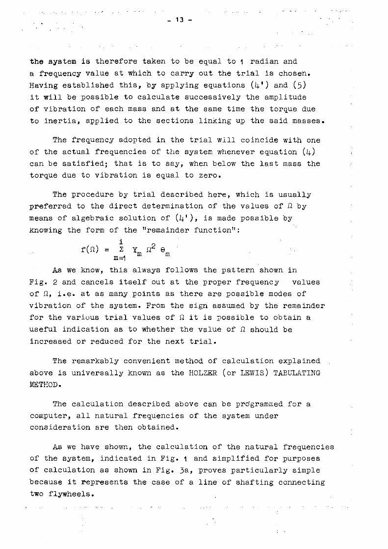
As we know, this always follows the pattern shown in

Fig. 2 and cancels itself out at the proper frequency values

of Ω, i.e. at as many points as there are possible modes of

vibration of the system. From the sign assumed by the remainder

for the various trial values of Ω it is possible to obtain a

useful indication as to whether the value of Ω should be

increased or reduced for the next trial.

The remarkably convenient method of calculation explained

above is universally known as the HÖLZER (or LEWIS) TABULATING

METHOD.

The calculation described above can be programmed for a

computer, all natural frequencies of the system under

consideration are then obtained.

As we have shown, the calculation of the natural frequencies

of the system, indicated in Fig. 1 and simplified for purposes

of calculation as shown in Fig. 3a, proves particularly simple

because it represents the case of a line of shafting connecting

two flywheels.

C.C.R. ISPRA

EURATOM

Fig. 2

C.CR. ISPRA

ÏG5

Φ^Ο

¿30

925

Φζο

¿18

Φ 15

*10 Γ.

di'10 JÎ

d f-S -

Φ3

d,-J

d¿ -10

Φ10 H

Φ20 r

4¿2

—ι m

Φ2Ζ r

^ ^

ΊΓ ^ — - ^ _ ^ _

^

! i

« ^ il

EURATOM

«

1

te

-5 M S!

sa ■s·

-S»

«S

~~-l

¡tf §" 1 -»

1 Ci

l l

ko

1 <=>

71 Ç\i

il

| ^

è

a) s V­II *

' — t

""" —■ s *

S

^—-—"—"£?

Í

w

Ci

-

r­

en

»

' 2Ä? _ j

1

Y*

m — · ^~[

Φ10

ε

1 Sí

m (D " ^ <u

b)

1

'

f tø 3 7.10S3/A-

- 16 -

In such cases equation (i+) gives, for the shaft section connecting the two flywheels:

*i Ω2 ©1 = *, (θ1 - θ2) where

G J ν- £ K1 - 1Ρ

is the torsional rigidity of the reduced system (see Fig. 3b)

From this we obtain

I 2 -1 - Ω2 (6) e1 κ,

On the other hand, equation (i+), when applied below the second flywheel, becomes

Y1 Ω2 θ + Y2 Ω2 θ2 = 0

Dividing by θ. , we get 1

Y1 Ω2 + Y2 Ω2 ^ = 0

stituting for θ?/θ , the value given by equation (6), we Sub obtain:

- ^ iL· - Ω2 (Υή + Y2) = 0

whence

Λΐ ^ 2 - Λ/ Y, Ya lr ( 7 )

This tells us that our system has only one natural frequency which we proceed to calculate (the double sign indicates that the flywheels can revolve in both directions).

­ 17 ­

With reference to the system shown in Fig. 3a, if we

reduce the lengths to an ideal diameter of 1 0 mm as described

in section 1.2 and allow for the correcting factors (ï ) in

respect of conical sections, joints and cross­sectional

variations in cylindrical sections, we get:

total reduced length: L a

1 ,280 cm

Our system is thus transformed, for the purpose of

calculating the torsional vibrations, into the equivalent

ideal system represented in Fig. 3b, in which

­ moment of inertia of mass (ï ) Y = 2.81 kgcm sec

­ moment of inertia of mass (2) Y? = 0.O106 kgcm sec

­ polar moment of inertia of

reduced shaft J = 0.098 cmr

Ρ , ρ

­ tangential elasticity modulus G = 850,000 kg/cm

Substituting these values in equation (7), we find

Ω = 78.5 rad/sec.

whence the only natural frequency of the system:

Ω χ 60

f = — 2 " ^ — = 750 /min

It may be objected that in calculating the system in

question, the actual mass of the shaft connecting the two

flywheels has not been taken into account.

It can be demonstrated that in order to,take account of

the mass of the shaft it is sufficient to add to the mass

moment of inertia of the nearest flywheel 1 /3 of the moment

of inertia of the shaft which goes from the said flywheel

to the nearest node. As may be verified, the latter moment

of inertia is very small compared with Y and Yp and is

therefore negligible.

>. 18 -

1 ·3·2 Determination of the critical torsional velocities

All velocities of the system under consideration which satisfy the relation

Fe = f = 750/min

are critical torsional velocities. Fe is the frequency of excitation of the system due to the electrical driving motor. This is a special high frequency synchronous motor with one pair of poles. It is started asynchronously and synchronized by manual frequency regulation at about 5OOO r.p.m.

It is known (2) that for a three-phase asynchronous motor, fed with a frequency F(Hz), the frequency of mechanical excitation is

Fe = 2(N - N)p S

where

Ν [rpm] = ve loc i ty of the revolving magnetic flux S

= 60 F/p Ν [rpm] = number of revolutions of the motor shaft ρ [-] = number of pole-pairs. Substituting Ν by its value and considering the first

relation and the fact that there is only one pole-pair, the equation for the critical torsional velocities of the system becomes :

Ν = 60 F - 375 (8)

During the asynchronous start-up procedure, it is therefore necessary to keep away from those frequencies by which the above equation can by satisfied, in order to avoid torsional vibrations which might cause a failure of the thin shaft.

­ 19 ­

Once arrived at synchronous operation, (~ 5000 r.p.m.),

mechanical excitation frequency Fe is zero as can easily be

seen from the expression for Fe, and therefore there are no

more critical velocities of torsion.

2. CALCULATION OF CRITICAL FLEXIONAL VELOCITIES

To simplify the calculation while still adhering very

closely to the real conditions, the system in Fig. 1 has

been reduced to that shown in Fig. ¿j..

For the reason given in the introduction, we shall con­

sider the three following cases:

(A) System as in Fig. 1+, loaded at its free end with the

rotor of weight Ρ = 30 Kg. The gyroscopic effet due

to the rotor and the traction effect due to the weight

of the rotor F = Ρ = 30 Kg are both ignored.

(B) System as above, taking into consideration the gyro­

scopic effect due to the rotor but ignoring the traction

effect.

(c) System as at (A) taking into consideration both the

gyroscopic and the traction effects.

The IBM 7090 computer was used for the solution of each

of these three cases, with which we shall now deal.

2.1 Calculation of the critical velocities of­the system

ignoring both gyroscopic and traction effects

We know that, in the case under consideration, the

basic equation for the critical velocities in respect of

a shaft, of constant cross­section, fixed only at its ends

and subjected to a uniformly­distributed load of weight ρ

C.C.R. ISPRA EURATOM

C ^ ^Ά I l ik

ff '24 SS

r

/ , ­ ß 5

■

i*· 32 ¿?

om

■fest 3

h- 25

i M'16

o *

*

a*

i t ­ J

"ΓΤ

s?

i o

ι

<5>

>

«M

«o

■

^.Z^L·* 4/5 cm*

ττ6,5*„ , 5Ζ - —;— ­ 33 cm*

V ¿t ir-3,2* „

Õ cm¡

S+'Z-^ïWcm*

V2

^ * # 4 cm*

V 2 ^ * 0,07cm*

57-Σψ-*3β cm2

1Γ-24*

ir-J,2u

J3—(tf-'ÏH-cm*

. fr-2,5**, Λ" ^4 ' 1-92cm

\mtJïT*0,3l cm*

h-^VT*'0fOO0U cm*

tr'221*

O LO

£

gy'22

x^omkg *m~ïm?-

981cm ^'~^c~r

rir2QQ0Û00kg L cm2

IX

Ρ - 30kg F'30 kg

Fig. 4 VfOS&í-

­ 21 ­

per unit of length, in the conditions assumed usually by

the analysis of stress and strain is (3) ­ (k) ~ (5) ­ (ï 1 ) ~

(12):

^ y u

= m'V (9)

with

cbA

»U

= f e do)

where :

ρ = SY = weight of shaft per unit length

S = cross­section of shaft

γ = specific gravity of shaft material

E = modulus of elasticity of shaft material

J = moment of inertia of cross­section of shaft

g = acceleration due to gravity

Ω = angular velocity of shaft.

The integral equation (9) has the value

y = A cosh m x+B sinh m x+C cos m x+D sin m χ (11 )

where A, B, C, D are constants which depend on the boundary

conditions.

Taking these into consideration we can always write a

sufficient number of equations containing the constants and

the mj we then cancel out the constant values and obtain an

equation in m whose solutions, substituted in equation (10),

enable us to find the critical velocities of the shaft.

In respect of a shaft made up of a number of lengths

of various diameter and fixed at several points, equation (11 )

is valid for each length and for each contiguous length con­

fined by a point of attachment; hence we must write as many

- 22 -

s e p a r a t e equa t ions as t h e r e a re l eng ths of d i f f e r e n t diameter and l e n g t h s conf ined by a p o i n t of a t tachment . In the case in q u e s t i o n ( F i g . 1+) denot ing wi th the ind ices 1 , 2, . . . , 7, the v a l u e s r e l a t i n g to the 1 s t , 2nd . . . 7th l eng th , we have the seven fo l lowing e q u a t i o n s :

y = A. cosh m. χ + BJ s inh mJ χ + C cos m. χ + D. s in m. χ 1 1 1 1 1 1 1 1

y = A2 cosh πΐρΧ + B? s inh m„x + C2 cos m?x + D2 s i n ni-x

(12)

m

y = Ay cosh m7x + B7 sinh m-,x+ C-, cos m-x + D-, sin m-x

Bearing in mind that the angular velocity Ω is common all the lengths and that it is related to the various m.

1 7 ; S. , . . . . , S 7 ; J. , . . . . , J-, by equat ion (ï θ ) , we can w r i t e :

m^E ^ g m^ E J 2 g m1^ E J^ g m^ E J^

^ γ s 2 γ =

s 3 γ =

s^ γ

n¿ E JV g mg E Jg g m E J 7 g

s 5 γ =

s 6 γ =

s ? γ

from which we o b t a i n :

k; S J m

2 =m

i J s f ^ = C p m

i

k S. J m

5 = m

i J Í J : = ξ ω

ι (13) l3 =

ω1 j S ^

= 1

ü ; S _ k A m, = m. Ι 0

Η τ' = τ m

­ 23 ­

Jr m5 =

mi 4 sfj^ ■ ψ ml

m6

= mi 4 ^ 1

= ^

( i3 )

m7

= mi J s ^ = " l

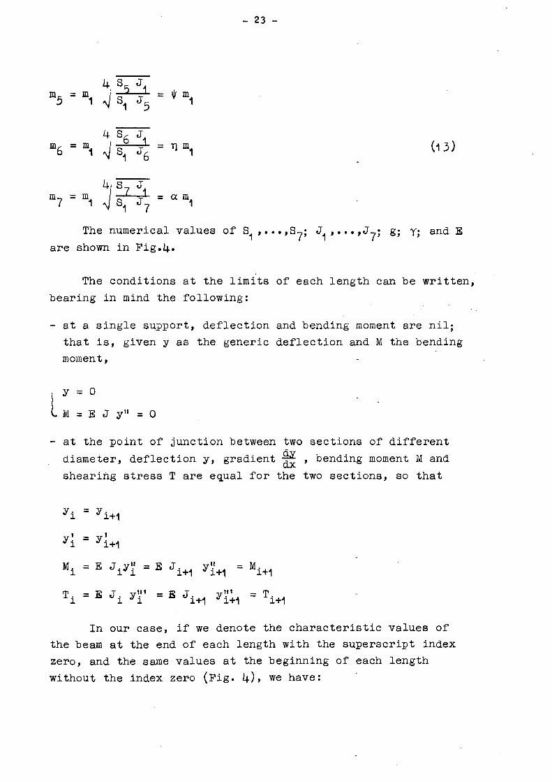
The numerical values of S ,...,S7; «Τ , ...,J7; g; γ; and E

are shown in Fig.¿4.·

The conditions at the limits of each length can be written,

bearing in mind the following:

­ at a single support, deflection and bending moment are nil;

that is, given y as the generic deflection and M the bending

moment,

y = 0

M = E J y" = 0 t ­ at the point of junction between two sections of different

diameter, deflection y, gradient g , bending moment M and

shearing stress T are equal for the two sections, so that

yi y

i+1

Yi ­ Yi+i

M, . E J^J = Β Ji+1 y»+1 = Mit1

T4 = E Jt y'}' = E Ji+1 y»^ = 1^

In our case, if we denote the characteristic values of

the beam at the end of each length with the superscript index

zero, and the same values at the beginning of each length

without the index zero (Fig. k)» we have:

­ 24 ­

(1 ) f o r χ = 0

[ y, = ο

y " = 0

(2) f o r χ = l t

o yi : y

2

s Ji Y°'

O

E J 2 y2'

LE ^ y f = E J2 y2"

(3 ) f o r χ = 1,

o y2

y3

o*_ , y2 "

y3

E J 2 y 2 E ¿y» ,111

^ E J 2 y ­ = E J 3 y J

(5) f o r χ = 1 h

»k = y

5

yk = y 5

E Jk y ° " = E J 5 y»

vE ·\ <" =

s J5

y5

M

(i+) f o r χ = 1 3

*3 = °

y u = 0

o' , y3

= y4

E J , y ° " = E J. y," V 3 "3

(6) f o r χ = 1

o : y 6

i,. %

5

o" , y 5 = y¿

E J y = E J 6 yg

, n i

VÎ J

5 y

5 = S J

6 y

6 I I I

(7) f o r χ = 1,

o y6

o' y6

= y7

= y7

E J 6 y6 = E J 7 y7 ,111

V

15 J ó y6 = E J 7 y7H

(8) f o r χ = 1 7

O " o

y 7 = o

o1" ._ k k o y 7 = R cT m^ y ?

The l a s t c o n d i t i o n a t t h e l i m i t s , f o r χ = 1 , can be

found , s i n c e we know ( r e f . 5) t h a t :

3­5 ­

E J7 y f = ­ P/g Ω2 y°

in which we substitute the value given by equation (9) for

Ω2, i.e.

­ S 7T

and, from the last of equations (l3), we obtain

0,„ ρ m^ E J7 g 0 Ρ (¿nfr 0

2 J7 y7 = ­ i s7 r

y7 = ­ ~Epr y

7

whence the said and last condition with

R = ­ φ = ­ 3.8 x°0.008 * ­

9 8 6 c m

Equations (1 2) and (13)> together with the conditions

at the limits of each length as written above, enable us to

write a homogeneous set of 28 equations in the 28 unknowns

A. · · · · A.­,, il, .... xj­7» L> .... 0­,, D. .... JJ­7 · 1 ( \ I 1 ( \ I

Having constructed the determinant of the coefficients,

we note that it is a function of the single parameter m ; for

all the values of this which cancel the determinant, (1 θ)

enables us to calculate the critical flexional angular

velocities Ω and hence the critical rpm values of our system.

The foregoing is the standard method of calculating the

critical flexional velocities. In practice it is difficult to

programme for the IBM 7090, so that we found it preferable,

from that standpoint, to use the method set out below as it

is far more convenient. It consists, very simply, in expressing

the final conditions of the beam in question as a function of

the initial conditions, taking into account the conditions at

the limits as written above. (For detailed explanation of the

method right up to the feeding into the IBM 7090, the reader

is referred to the report by Messrs. M0NTER0SS0 and DI COLA,

not yet published).

­ 26 ­

E q u a t i o n ( 9 ) , a p p l i e d to t h e 1 s t beam s e c t i o n , g i v e s

y = A, cosh m χ + Β, s i n h m, χ + C, cos m. χ + D. s i n m χ (l¿+) 1 1 1 1 1 1 1 1

I t s s u c c e s s i v e d e r i v a t i v e s up to t h e t h i r d , have t h e v a l u e s

y ' = m. A, s i n h m., χ + mJ Β„ cosh m, χ ­1 1 1 1 1 1

­ m. C, s i n m χ + πι, D cos m, χ 1 1 1 1 1 1

2 y" = m. A, cos h ι , χ + m, B s i n h πι χ ­

1 1 1 1 1 1

2 2 (15) ­ πι, C cos πι χ ­ πι, D, s i n πι χ

1 1 1 1 1 1

y'" = nr Α„ s i n h πι χ + mj Β, cosh m, χ + 1 1 1 1 1 1

5 '5 + nr C. s i n πι χ ­ nr D. cos m. χ

1 1 1 1 1 1

The s e t formed from (14) and (1 3) f o r χ = 0 g i v e s :

yi

'Í

y ;

v1"

= A

1

= mi

- <

..>

+

B1

A1

B1

°1

+

­

­

mi

<

«Ì

D,

C1

D1

(16)

where y , y ' , y " , y"1 a r e t h e i n i t i a l c o n d i t i o n s of the beam.

D e r i v i n g A. , Β , CÁ , D, from t h i s s e t and s u b s t i t u t i n g 1 1 1 1 e

them i n t h e s e t formed from (14) and (15) we o b t a i n , f o r

x = V

y° = y, 2 ^c o s h m

i χ

ι ) + y

i Fm" ^s i n h m

i \ + s i n m

* 1

1 ) +

+ y" —L­r (cosh m 1 ­ cos m 1 ) + y'" —J­τ­ > 1 2 mf

η η 1 1 1 2 nr

5

1 1

(sinh m χ ­ sin m χ)

­ 27 ­

= y«, 2 ( s i n h m1 1 ­ s i n m 1 ) + y ' .£ ( c o s h m 1 +

+ cos m. 1 ) + y" ­r — ( s i n h m. 1 + s i n πι 1 ) + 1 1 1 ¿m 1 1 1 1

+ yJ" — ci> ( c o s h m χ ­ cos m χ ) 1 2 m; 1 1

yl = y

i 2 ^C O S h m

i Χ

1 " COS m

i "S ) + y

1 2 ^S i n h m

l Χ

1 "

­ s i n m, 1, ) + y," o ( c o s h m., 1 + cos m. 1„ ) + 1 1 1 ¿ 1 1 1 1

+ yì" 2~m~ (

S i n h mi "S

+ s i n mi X

1 ^

m 3

m. y1 = y l 2 ^ S i n h mi 11 + S i n m i lj\ ' + y l 2 ^ C 0 S h mi X1 *

m ­ cos m. 1. ) + y." -£■ (sinh m. 1, ­ sin m. 1. ) +

1 1 i ¿ 1 1 1 1

+ y'" τ: (cosh m. 1. + cos m. 1. ) . 2 1 1 1 1 1

Bearing in mind the above­mentioned conditions at the

limits for the point χ = 0, we get:

ε IO

» ■ ·

ε •c c

^ ­

ε s o

* ■ > · .

if ■c •0 o

­tr

­ N

Γ c

+

•c c

^>­

ε~ <0 o o +

" * p * ~

ε ■c •0 o

IO o o

ε .C ίο

«o o o ·§

•o

4V ~ ' < \ l

ε ■C

c

ε

•c «o o o

­h

ε .c

εΊ^

ε .c

■c

«o

H 6

<0 O

o

ε •c o o

ε~ .c <o I

F ­c c

rL

10 o o 1

—*"

ε~ ■c 10 o

tf*

fc: •0

o o ■»■

» ■ »

ε~ x­

—(C

OS

i

2

V

ε c ¡Ò 1

—.—

ε" ■c

c

ε>· ­ β

ε «0 o o l „

ε~ •c o

ε |M M s " o

c

ε .ς ί) + *

ε~ •C

Ί Ε Ί Μ « ο * Γ

­ 29 ­

which represent the value and respective derivatives of y at

the end of the first beam­length as a function of the initial

conditions.

For the second beam­length, we get:

y s A? cosh m„ χ + B2 sinh m χ + G eos m χ. + D2 sin m2 x

y' = m? A sinh m2 χ + m2 Β cosh m χ ­ m C sin nu χ +

+ m2 D cos m χ

2 2 y" = m„ A0 cosh m0 χ + m„ Β sinh m0 χ ­2 2 2 2 2 ¿ (18)

2 2

­ m? C2 cos m2 χ ­ m„ D2 sin m χ

y'" = m2 A2 sinh m2 χ + m£ B2 cosh m2 χ +

λ 5

+ m2 C2 sin m2 χ ­ m2 Dg cos m2 χ

When χ =1., we obtain 1

y = A cosh m 1 + B2 sinh m£ 1 + C2 cos m2 1 + D2 sin m2 1

y' = m A2 sinh m 1 + m2 Bg cosh mg 1 ­ m2 C2 sin m2 lg +

+ m2 D2 cos m2 1

y» = m2 A2 cosh mg 1 + m2 B2 sinh m2 XJ| ­

­ m2 C2 cos m2 1 ­ m2 D2 sin m2 1^

y2" = m3 A 2 sinh mg 1 + m­3 Bg cosh m,¿ 1 +

+ m^ C2 sin m2 1 ­ m| D2 cos m£ 1

Deriving A?, B?, C2, D from this set and substituting

in equation

transformations :

them in equations (l8), we obtain for χ = 1 , after certain

ι—ZT

¿«N

ε •s «o

ε" «O

o

I

C

Ό

¿«Ν

10 ο ο

_ . « Ν

c

3 1 ι

<Ν

ε ο ο ι

Ν —

ε"

J

+

¿«Ν

ε* c «ο

+

<Ν

ε

s

ii

ε" Ο Ο

+

^_<Ν

10 ο υ

S3 '

s*.

ε ς

ε 10 Ο

€ Λ* ε •c

+

<Ν

ε" -c «ο ο Ο -Je*

c

εμ

ε" c «ο +

<Ν

«ο ο ο

ε" c 10 ι

ε" 10 ο ο ι

ε c

- β

+

ε «ο ο ο

ι ON

ε c ·—» 10

1 ñ Ι ε ι CM

χ*

ε

εκ

V

<0 ο ο ■f

—/Ν

Ν * ­

ε" ο ο

ε c

ι

O1·

­C

c

εΊ Il

V

Ρ,

ε" «ο ο υ

<Ν

ε" 10 ο Ü

Th SS«N

'o »

­i«N

ε" c <0

+

­% ^.·~ ■i"· ν ­

ε" Ι C

·— ι

Ι «ο Ι

* < Ν

c <b

* * Μ

·*» ^ ^

Ο* •Q

C «S O

■c

­c ^

Oí

VJ

I ­ . 1 "N '

ε" c IO

I — χ

■Ι *

ε" ?

| Ä ι

­Κ"

ι ^ ι ι

­ ο *

£■ <0 ο ο

­ Ν

­1<Ν

■c «0

Ι S I r ι / _ I 1 ρ­ I

J.CN

ε" c V)

*

1 — « Ν

ε­■c c

ι 'iõ I ' Α .

­lí

1­3. I I

­JM

«o· o

υ

+

­ Ν

I

il ι S ι «­ρ

*

1 ­s I I ^ ­ 1 Í N

υ ι

,_ ·~

ET •c vt

1 ° 1 1 SL '

­ f t "

Ι Ξ­Ι ­S E­

c vt

Ξ­­S

Í 1 |j

HE

Ι "Ν 1 1 ­ ­ |

­¿.•N * ■

10

o u ♦

| ·—<N

ET ■c vt

ι 2 1 υ I

— | < M

I 1 1 ­> ι

1

ET C Í

' " Ν

ir ■c

ι S ι 1 — ¡ ς ? — ' ε) «ν,

m V·

ι ι I ' -Ν

'T c

* ■ - * s

¿Ν

L2U

­Id

1 ­» I —r. '

•¿■Ν v—

ET IO

o o +

I

­1·Ν

ε" ■c

ι ">

Ι s ι — | < Ν

Ι ι Ι

"Ν - * . * * ■

•^.Μ

ε" .C vi

Ι

Ι

Ε" ■c

Ι S Ι Ι vi ι

sta

Ι ­ Ι ι ι

ι ­JN

ε­vt Ο υ ι

­ - j -

ε •ο

Ι s ι m<N

»ο

V

Ι ^J

Ι*. «0 ο ο +

"Ν

·*β·­

χ; 10

Ι ? Ι Ι ο­ Ι

—.|<Ν

| ­%__ |

— < Ν

ir c vt

ι

I —"Ν

­

ι c

1 3 ι eh

ι ­*» ι Ι ^­ ι «L«N

ir 10

o o 1

~­

~."N

ε" 10

1 ° 1 1 o 1

th

| ^ |

­i.­ε" c £5

■c c

1 'iõ I

th

'°~ $

• . 4ι i .

Õ)

^

£ Ο)

c dl

Οι

Ο

m |

<b

£

(O

C

o ■ · —

■Q

C o o 0>

•C 1—

Ό M

5<-

H > H ^

S*s¡

»?

«o

«O

0i

­C

.«o

s I

o _ i,

SC

■ b

πζ—ι

c UI

UI O O

I UI

S3

E

c

ΙΛ

E c UI

UI o o I

c UI

+

UI o υ 4­

. Γ ­

­α

o

UI ui Ol

O L

Χ Ol

OJ ­ C ■ * - <

Χ ) c

σι c ω

—'

F π ω

­α

TJ

(_ ο

ï UI

Ol j r

c UI

m OJ

­ IE

CM

UI O O

J ΓνΙΓ­Ι

­ IE

CM

C

UI

r ­ E

UI

o

I ° I

­h

c UI

Ul O o

UI

o

II

E c UI

+

Χ

c

­ ε (NI

ω o o

ui o u

ç UI

I

TD C

σι c u σ οι

χι

­α cr □

CL

n

c o

Ul Ul 01 ι­Ο . X u

c

■ CM

=­>

­ r­J

>­.

­ P<

><

> N

Ι ­

Ο M—

. o CM

C

o UI UI OJ

L· α­χ ω

UI Ol

>

σ

> Ι ­

ΟΙ

­σ

ΟΙ

> ·*-. υ οι α. UI οι Ì-

-σ c σ

0) η

σ

>

οι χ

c

σ

X I ο

οι

ιη c ο

U

c ο ( Ι

, ο

c

01 Γ

-^ Η ­

ο

σι ,

.Ε V ~ fe­■Μ >>

xl ­ω >>

m

c o

u c η

UI o u

χ: UI o

HE

ΓΜ

UI

+

χ: c

UI

o

χ : UI o

I » I

Η Ν

E c

E χ c

J L

UI

o

UI o υ

c UI

I

χ c

Νι

E|c

UI o υ

+

E

c

c Ul

Ek

o o

Eh

c Ul

" l

E ir

-\ Γ

UI

o o

Ul

o

I " I

E|c

Ί Γ

Ul o u 1

c Ul

+

E X c

E|CM

UI o (J

- I E

c UI

-iE CM

Ul O O

-(CM

C 'ui

χ c

^ Ε

UI o o

X Ul o o

E CM

Ul o u

X Ul o o

E cr

'ui

E χ c UI

Eh

UI o o I

X Ul o u

£CM

c

Eh

Ul o υ I

X c Ul

X Ul o υ

"É>

c Ul

c 'ui

"Er­

•—» I»—>

»­.|»—ι

­ 33

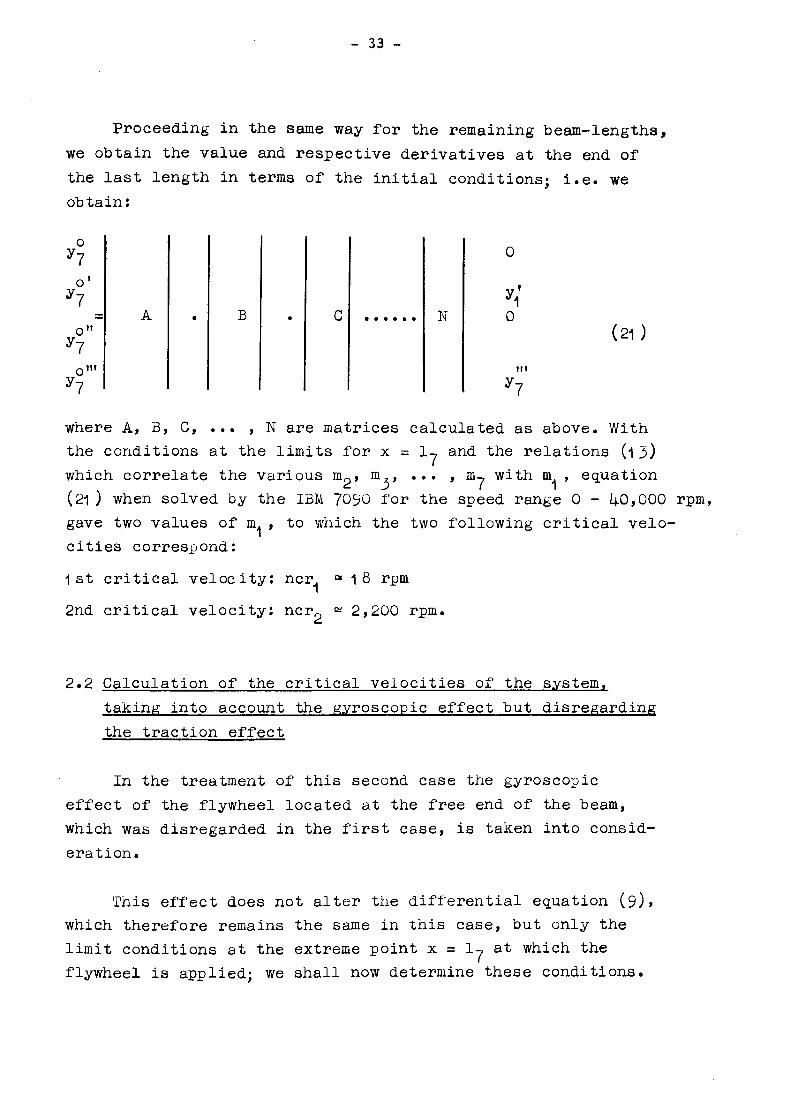
Proceeding in the same way for the remaining beam­lengths,

we obtain the value and respective derivatives at the end of

the last length in terms of the initial conditions; i.e. we

obtain:

'7

1

It

III

A • Β • c Ν

0

0

III

(21)

where A, B, C, Ν are matrices calculated as above. With

the conditions at the limits for χ = 1­, and the relations (ï 3)

which correlate the various m2, m,, ... , m? with m , equation

(21 ) when solved by the IBM 7090 for the speed range 0 ­ 40,000 rpm,

gave two values of m , to which the two following critical velo­

cities correspond:

1st critical velocity: ncr « 1 8 rpm

2nd critical velocity: ncr„ ­ 2,200 rpm.

2.2 Calculation of the critical velocities of the system,

taking into account the gyroscopic effect but disregarding

the traction effect

In the treatment of this second case the gyroscopic

effect of the flywheel located at the free end of the beam,

which was disregarded in the first case, is taken into consid­

eration.

This effect does not alter the differential equation (9),

which therefore remains the same in this case, but only the

limit conditions at the extreme point χ = ly at which the

flywheel is applied; we shall now determine these conditions.

­ 34 ­

In cases where concentrated loads such as pulleys or fly­

wheels are applied to a shaft, when writing the equations at

the limits for two contiguous lengths limited by a load, we

must bear in mind not only that the ordinates and the gradients

of the elastic curve and the shearing stresses, as calculated

from the two equations relating to the two lengths, must work

out equal, but also that there exists between the moments

calculated below and above the loaded section the relation

Mv­ Mm = Ω2 P/g p

2 y' (22)

2 where P, g,Sl have the same meaning as before and ρ is the

radius of gyration of the flywheel or pulley.

In our case, since the flywheel is at the free end of

the beam, (22) is reduced to

­ Mm = Ω2 P/g p

2 y°'

and, replacing M by its value,

n" 9 ο ,Λ« 4 E J 7 g Ρ 0 , E J?y°7 = ­ n 2 p / g p 2 y o = ­ ­ J _ L _ p 2 y ?

7

i.e.

c m^ Ρ ρ2

o ' ττ U U o ' ζ x y7 = ^~1 y7 = H m y

7 (23)

where :

g Y 981 χ 2.81 p = IP * 2 χ 30 " ^ cm

Η « ­ £­¿ * 3° χ ¿+

6 « ¿,5 500 cm

3

η S­, Υ 4.16 χ 0.008 ^,^υυ

cm

The limit conditions for

x . l 7

are therefore in this second case

­ 35 ­

y°" = H cl·

y°'" = R c^

4 0* m1

y7

k o m

l y

7

(24)

When the calculation was made on the IBM 7090 as described

in section 2.1, equations (24) being now substituted for the limit

conditions at the point χ = 1­,, the following were found for

the velocity range 0 ­ 40,000 rpm:

first critical velocity: ncr = 20 rpm

second critical velocity: ncr? = 29»500 rpm

This result shows that the gyroscopic effect has very

little influence on the first critical flexional velocity but

causes a large increase in the second critical velocity,

raising it from the 2,200 rpm of section 2.1 to 29»500 rpm.

2.3 Calculation of the critical velocities of the system,

taking both the gyroscopic and the traction effects

into account

In this case account is talven of the gyroscopic effect

due to the flywheel of weight Ρ = 30 kg located at the end

of the shaft and the effect due to the pull of the force

Ρ = 30 kg (weight of rotor). The differential equation for

each beam­length now has the form:

äk ν d

2 ν S Y 2 ^ * ( 5 )

/ Ν

d x4 d x g

whose integral is

mIx . m I ] : x m I ] : I x . mlV y = a e + b e + c e + d e χ

where m m are the roots of the equation:

4 2 S γ Ω2

E J mH ­ P m ­ = 0

- 36 -

i.e.

m Γ~

Ρ 2 Ε J " .

Ι Ρ 2 + S Υ Ω2

J 4 Ε2 J2 g Ε J (Ι, II, III, IV) β ± F ± Εΐ_ + S Υ Ω (2Ó)

Prom this relation it can be seen that there are two

equal real roots of opposite sign, which we call respectively

m and -m, and two equal and opposite imaginary roots, which

we call ir and -ir.

The integral of equation (25) then becomes

mx , -mx ir , -ir y = a e + b e + c e +de

from which, making the appropriate changes, we obtain the

equation:

y = A cosh mx + Β sinh mx + C cos r χ + D sin rx

which is valid for each of the seven sections that make up

the system under study.

The conditions at the limits of each section are the

same as in section 2.1, wi th the exception of those relating

to the point χ = ly, which has now become:

Β J7 y°" = - Ω2 P/g p

2 y°'

o '" 2 o o '

E J7 y° = - P/g sr y° + Ρ y°

o'

(27)

The term F y? represents the component of the pull in

the direction of the y axis at the point χ = 1 . It is opposite

Ρ 2 o '

to the centrifugal force — Ω y due to the flywheel of weight P.

Applying the method of calculation shown in section 2.1 we

find, as far as the second beam-section:

(r2* mp

r2 coshm2( l- /, ; * ιτζο osy I- /; ; (r¡.m¡J m

2 2

^— sinhm/l2- lfJ*-^-sinrjl-IJ r2

2 2 I

fi* "if coshmjl- I) -cos ς(Ι- y

(FTTñp -¡-sinhmU2-l,)-±-s¡nr2<t-,> 1 O O O

™2Γ2

(r2* mp

r2sinhmfi2- t,)-m2sinr2( l2- lt) ( r/* mp

r2 coshmjlf μ *m2cosr2(l2- ^

( r2* mp

m2sinhm/ lf Ç*r2sinr2(l2-/, j (r

2* m¡)

coshmj^-l,)- cos r2 l2- /, ) 0 1 0 0

m2

r2

2

(φ m~[)

2 2 m2jj__

(r;*nf)

coshm2(l2- tjj - c osr2( t2- /;J

mjiinhmjlj- { )+r2sìnr2(l2- μ

m2r2

(r2*m¡)

2 2 1712^2

rrf+ mp

r2sinhm2(l2- ¡J-rnsinrj^- / ; ;

coshm2(l2-(¡)-coscit2- lt)

( r2* m

2J

2 2

mfoshmJI2- l^+qcostfl- Ç — 1 — _ m^inhrnf l- l^hr^inrj l}- t A

F7f~mjj m2sinh mJL,-^)- çsinrj l- /; ; ^ —J T "V coshmd- I )*rcosr(l -I

2 2 1 2 2 2 ' Λ

0 0 - ^ - 0 J2

0 0 0

1 2 2

(rcosh mi* m.cos ri) rf* mf ' " ' ' '

m2 r

' 2 (^sinhm^-mfinr^ ; r, * m,

2 2

2' 's (coshmflr cosr^) rt* m,

2 2

1 (m,sinhm,l,* nsinr U —= τ- ι ιιι,Λΐιαιιη,ι.* ι äinr ι/

rf* m2 I I I I

1 r2 . mf

(-^rSinhml+-—¡- sm rl ) 1 i Γι 11

η * m- m

i

; * 2

( r cosh mi * mcosrlj r

2* m

2 ' ' ' ' ' '

η + m,

m,2 Γ

'2 r rtsinhmflr- msinr^J ri + m

.

2 2

—i—'·—γ (coshrnl-cosrlj η * rn-j

Ί ' ' '

— r Í cosh ml - cos rl J rf * m' ' ' ' '

-r--Jtm1slnhmt1*rtsinrttí) r, * m,

1 , 2 2

2 i tm^oshm^^qcosr^J r, *m,

pi m2 (mfsinmf,-r;sinr,l,) ? . .

^ L ^ f ^ s i r t h m ^ - l - s i n r ^

(coshml- cosrl J .2 „ 2 " ' '

r'.w2 (m

tsinh

'"Vi* r

isin

W

' 2 2 —5 γ (mcoshml* r cosrl) rr * rrr ' ' ' ' ' '

y

y.

- 39 -

Proceeding in the same way with the remaining lengths we arrive at an expression similar to (21 ) which gives us the value and respective derivatives of y at the end of the last length as a function of the initial conditions.

Associating with it the limit conditions (27) and the expressions for m m? and r r? given by (2b), the IBM 7090 supplied the two velocities below, for the velocity range 0-40,000 rpm: first critical velocity: n cr * 64 rpm second critical velocity: n cr? - 29,500 rpm

This result shows that the traction Ρ changes only the first critical velocity and does not affect the second critical velocity of the system, or rather, its influence on the second critical velocity is very small as compared with that of the gyroscopic effect. Actually, when a calculation was made of the system taking traction effect but not the gyroscopic effect into account, we obtained: first critical velocity: η cr - 62 rpm second critical velocity: η cr2 - 2,800 rpm

3. CALCULATION OP THE CRITICAL PRECESSION VELOCITIES

The portion of shaft above the small-diameter (3mm) section (see Pig. 1 ) is extremely rigid with respect to the latter; this is confirmed by calculation and by tests conducted on the rotating system up to failure of the narrow-section.

Hence, for the purpose of calculating the critical precession velocities, no appreciable error will be made by adopting the simplified system shown in Pig. 5·

EURATOM

í­i m m

Λ ¿¿-¿i'120 mm

h § = 22 mm

Li' 175 mm

¿2 · 235 mm

FIG. 5

b) FIG. 6

yDsi

FIG. β

-Yd β ω (2 Si-ω)

Ρ-30 kg

-Υάωβ(2&-υ))

meo2 y

-41--

For the sake of clarity we have thought it advisable here to set out this calculation in three parts, as follows

(A) calculation of the moment of the forces transmitted from the rotor to the shaft;

(Β) equation and calculation of the precession velocities;

(C) determination of the critical precession velocities.

These are dealt with below.

3·1 Calculation of the moment of the forces transmitted from the rotor to the shaft

For the calculation of the critical velocities of bending it was assumed that the rotational speed of the system around the distorted axis is the same as the speed around the straight-lined original axis.

Let us assume now the shaft-rotor system in Fig. 5 has the following velocities:

- precession velocity ω, at which the axis of the shaft, distorted as shown in Fig. 6a, rotates anti-clockwise round the axis OB which corresponds to its non-distorted position;

- rotational velocity Ω around the distorted axis OC, in the same direction as the precession.

Owing to these velocities, the rotor is subjected to two different moments of momentum, which will be calculated separately.

Let us suppose that ω = 0 and Ω ^ 0.

^ 42 ­

The rotor will then turn without precession around the

deformed axis OC so that, given Y as its polar moment of

inertia with respect to axis OC its angular momentum is the

vector Υ Ω perpendicular to the plane of the rotor and

having the direction shown in Fig. 6a.

If Ω = 0 and ω ¿ 0 the rotor is subjected to two

rotations: one together with the shaft, with angular velocity

ω, around the axis OB, its centre of gravity C describing a

circle with centre Β and radius y, and the other, with angular

velocity μ, around one of its diameters which is perpendicular

at C to AC which is perpendicular to the mean plane of the

rotor, the shaft always remaining perpendicular at C to the

rotor during precession.

The first rotation sets up the centrifugal force m ω2 y

(Pig. 7), m being the rotor mass; while the second causes the

angular momentum due to precession.

The latter moment is the product of μ Y,, where Y, is

the moment of inertia of the rotor respect to its diameter.

Let ;

disc

Let us calculate the values of μ and Y,. In the case of a thin

Yd = V

2

a relation which is sufficiently applicable to the rotor under

consideration. The angular velocity μ of the rotor is not so

easy to calculate.

Bearing in mind, however, that during precession the shaft

always remains perpendicular at C to the rotor, we see that the

straight line AC (perpendicular to the rotor), forming the

angle β with the axis OB, rotates at the same angular velocity

μ as the rotor. Thus if we determine the angular velocity of AC

we shall have found that of the rotor. As it moves, the straight

- 43 -

line AC describes a cone, with vertex A, and its end C has a velocity of ω y.

At time t = 0, shown in Pig. 6a, the straight line AC is in the plane of the diagram and the velocity of its point C is perpendicular to the latter. After a time dt, point C is lower than the plane of the diagram by the quantity ω y d t. The angle between the two positions of the straight line AC is then ω y d t/AC and since y/AC = β, if β is small, the angle through which AC rotates in the time dt is ω β d t, and the angular velocity of the straight line AC (and so of the rotor) is

μ = ω β

The angular momentum due to precession is then the vector Υ, ω β, having the direction and sense indicated in Pig. 6a.

Let us break down each of the angular momentum vectors Υ Ω and Υ, ω β into the two components (Pig. 6b) parallel and perpendicular to the axis OB. The total angular momentum to which the rotor is subjected is given by the two vectors

Υ Ω cos β + Υ, ω β sin β parallel to axis OB

Υ Ω sin β - Y, ω β cos β perpendicular to axis OB

Where β is assumed to be small, these become respectively:

Υ Ω + Υ, ω β2 parallel to ax-is OB

Υ Ω β - Yd ω β = Yd β(2 Ω-ω) perpendicular to axis OB ±J KJ. \A.

The first (parallel to axis OB) rotates parallel to itself around the axis OB, describing a circle of radius Y, and its length remains invariable throughout its movement, so that its derivative with respect to time is zero.

- 44 -

The second (perpendicular to the axis OB), on the other hand, describes a circle with centre Β as it rotates. At time t = 0, this vector is in the plane of the diagram; after a time dt it forms a downward angle of ω dt with this plane.

It thus undergoes a variation given by the product of this vector and ω dt, which is

Yd β(2Ω-ω)ω dt

The derivative of this vector with respect to time is

Yd β(2Ω-ω)ω

So this expression represents the derivative with respect to time of the total angular momentum to which the rotor is subjected.

According to the familiar theorem of angular momentum of rational mechanics (Ref. 6), the above expression is equal to the moment of the forces transmitted from the shaft to the rotor and so, by the law of action and reaction, equal and opposite to the moment of the forces transmitted from the rotor to the shaft, i.e. the couple the direction of which is shown in Pig. 7·

3.2 Equation and calculation of the precession velocities

On the assumption always made, likening the rotor to a thin disc, the following forces are applied to the end of the shaft to which it is attached: - the moment - Υ, βω(2Ω-ω)

2 - the centrifugal force m ω y - the traction force Ρ = Ρ = 30 kg due to the weight Ρ of the rotor when the system is in the vertical position.

­ 45 ­

The last­named force gives the component Ρ β (Fig. 8)

which is perpendicular to the axis OB, and is constantly

opposite to the centrifugal force m ω y.

Denoting by:

α. the deflection of the shaft at the free end where the 11

disc is attached, due to the application of a unit load

at that point;

QL 2 the deflection of the shaft at the free end, due to the

application of a unit moment at that point; or the angle

formed by the shaft with the axis OB at the free end,

due to the application of a unit moment at that point;

ou2 the angle formed by the shaft with the axis OB at the

free end, due to the application of a unit moment at

that point;

and ignoring the mass of the shaft (with respect to that of

the rotor), we have the following shaft distortion equations

(Fig. 8):

y = o^ m ω2 y ­ α, Ρ β ­ α Yd ω β(2Ω­ω)

β = α, 2 m ω2 y ­ α, 2 Ρ β ­ α ^ Y ¿ ω β(2Ω­ω)

we now find y/ß from the first and second equation and equate

the results, so that we have:

o^P + ai2 Yd ω(2Ω­ω) 1 + OL g Ρ + ag2 Y¿ ω(2Ω­ω)

2 ~ 2

OL . m ω ­ 1 CL 2 m Gu­

By eliminating the denominators and arranging the terms in

descending order of powers of ω, we obtain the expression:

u>\­m o5j1 a22 Yd + m α22 Yd) + u>3(m a^ QL^ Yd 2Ω ­

­ ma22 Yd 2Ω) + ω 2 (α 2 2 Yd + moj|J| ) + ω( ­α 2 2 Yd 2Ω.) ­ (ï + ^ g P) ·= 0

which is the equation for the precession velocity.

­ 46 ­

This, it will be observed, is an algebraic equation of

the fourth degree in ω, so that for a given shaft supporting

at its end a given rotor and rotating at a certain velocity Ω,

there are four characteristic precession velocities.

The system in question therefore has, for any Ω, four

precession velocities which will now be calculated.

V/ith reference to Fig. 5, the values to be introduced

into the equation for the calculation of the precession

velocities are:

p

m = P/g * O.O306 Kg sec /cm

Yd = Y /2 * 1 .405 Kg cm sec2

6 ? E ="2x10 Kg/cm (modulus of elasticity of shaft material)

J. * 1 .1 5 cnT" (moment of inertia of 22 mm diameter shaft­section) 1

J a

O.OOO4 cnr" (moment of inertia of 3 mm diameter shaft­section)

.J l3 - 13> ai1 = 3

,1.3 1¿ ­ l3.

(1 ­ 1 )2 (1 ­ 1)1 l

2

a = — ύ 3 + — - ] L + J « O.352 1 ¿ 2 E J2 E J2 2 E J

a22 = u f

+ f j ; ^ ° ·

0 1 5

On the basis of these values, the precession­velocity equation

for our chopper­rotor is:

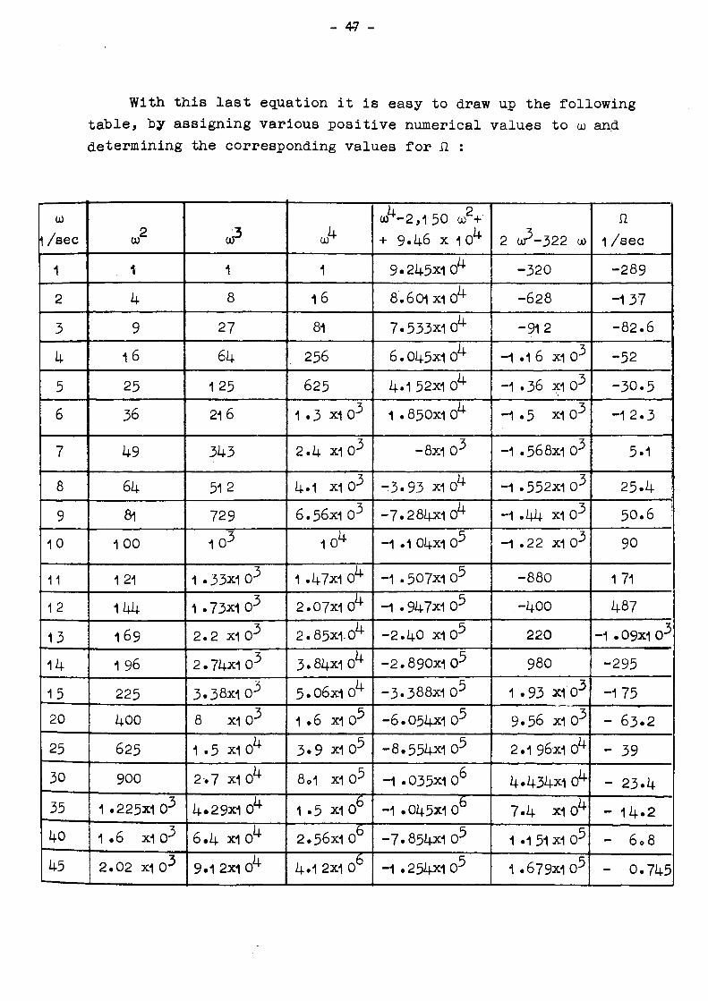
ω^ ­ 2Ω cx)3 ­ 2,150 ω2 + 322 Ωω + 94,6θΟ = 0

The numerical solution of this equation is time­consuming and

it is therefore better to transform it into the following:

n . ^ ­ ΖΔ 50 ω2 + 94.600

2 ütf5 ­ 322 ω

solving for Ω.

- 47 -

With this last equation it is easy to draw up the following table, by assigning various positive numerical values to ω and determining the corresponding values for Ω :

ω 1 / sec

1

2

3

k

5

6

7

8

9

10

11

12

13

14

15

20

25

30

35

ko

k5

ω2

1

k

9

16

25

36

49

64

8i

100

121

144

169

196

225

400

625

900

1.225x1 o·5

1 .6 x l 0 3

2 .02 X 1 0 3

oP

1

8

27

64

125

216

343

512

729

1 0 3

1 . 3 3 x 1 ο 3

1 .73x1 O3

2 . 2 X10 3

2.74x1 o 3

3 . 3 8 X I O 3

8 X10 3

1 · 5 X10^

2 . 7 X10^

4 · 29x1 cl·

6 . 4 X10^

9.1 2x1 0^

ul· 1

16

81

256

625

1 . 3 X10 3

2 . 4 X10 3

4.1 x l o 3

6.56x1 o 3

1C*

1 .47x1 0k

2 . 0 7 x 1 0 ^

2 . 8 5 x 1 0 ^

3 . 8 4 x 1 0 ^

5.06x1ο1 4

1 .6 x l O5

3 . 9 X10 5

8.1 x l O3

1 .5 X10 6

2.56X10

4.1 2x1 0 °

4 2 ( iT-2 ,1 50 ω + + 9 .46 χ 1 0^

9 .245x10^

8 .601X10^

7 .533x10^

6.045x1 cl·

4.1 52x1 cl·

1 .850x1 cl·

-8x1 O3

- 3 . 9 3 wel· - 7 . 2 8 4 x 1 0 ^

- 1 . 1 04x10 3

- 1 . 5 0 7 x 1 o 5

-1 .947x1 O5

- 2 . 4 O X10 3

- 2 . 8 9 0 x 1 O3

- 3 . 3 8 8 x 1 o 3

- 6 . 0 5 4 X 1 0 3

- 8 .554x1 o 3

- 1 . 0 3 5 x 1 o 6

- 1 . 0 4 5 x 1 0

- 7 . 8 5 4 x 1 o 3

- 1 . 2 5 4 x 1 o 3

2 ω 3 -322 ω

- 3 2 0

-628

-912

-1 .1 6 x l O3

- 1 . 3 6 X1 O3

- 1 . 5 X10 3

- 1 . 5 6 8 x 1 0 3

- 1 . 5 5 2 x 1 o 3

- 1 . 4 4 X1 o 3

-1 .22 X1 O3

- 8 8 0

-400

220

980

1 . 9 3 X10 3

9.56 X10 3

2.1 96x1 CT"

4 .434x1 el·

7 .4 X 1 0 4

1.151 χ ι o 3

1 .679x1o 3

Ω

1 / s e c

- 2 8 9

- 1 3 7

- 8 2 . 6

- 5 2

- 3 O . 5

- 1 2 . 3

5.1

2 5 . k

5 0 . 6 !

90

171

487

- 1 . 0 9 x 1 o 3

- 2 9 5

-175

- 6 3 . 2

- 39

- 2 3 . 4

- 1 4 . 2

- 608

- 0 .745

GÚ

1 / s e c

50

60

70

80

90

1 00

150

200

250

300

350

400

4 5 0

500

6oo

700

800

900

1000

]

ω2

2 . 5 Χ1 O3

3 . 6 χι Ο3

4 · 9 Χ1 Ο3

6.4 xi Ο3

8.1 χ1 Ο3

101*

2.25x1 Ο1*

4 χ ί ο ^

6.25x1 Ο14-

9 Χ1 cl· 1 .225x105

1 .6 Χ10 3

2.02X1 Ο3

2 . 5 Χ1 Ο3

3 .6 χ1 Ο3

4 . 9 χι ο 3

6 . 4 Χ1 Ο3

8.1 Χ1 Ο3

1 0f a

?or v a l u e s c

rhe v a l u e s i rounded o f f .

co2

1 .25x1 0 3

2.1 6x1 0 3

3.43x1 o 3

5.1 0x1 O3

7 . 3 X10 3

10fc

3-37x1 O6

8 X106

1 .57x1 O7

2 . 7 X1 O7

4.28x1 O7

6 . 4 X1 O7

9.1 2x1 O7

Q

1 .25x1 0 Q

2.1 6x1 0

3.43x1 O8

5.1 2x1 O8

7 . 3 X108

109

)f ω > 1 ,00(

.n t h i s t a b

- 48 -

u/*

6.25x1 0

1 . 3 X107

2 . 4 X107

4·1 χι o 7

6.56x1 O7

, 0 8

5.06x1 0

1 .6 xl O9

3.91x1 o 9

8.1 xl O9

1 . 5 X 1 0 1 0

1 0 2.56x1 O1

4.1 2x1 O 1 0

6.25x1 o 1 0

1 . 3 X1011

2 . 4 X1011

4.1 X1011

6.56x1 O11

1 0 1 2

D, Ω * ω/2

Le were cal<

4 2 ω - 2 , 1 50 ω + + 9.46 χ 1 0^

9.746x1 O3

5.354x1 O6

1.354x1ο7

2.731X1 O7

4 .827X10 7

7.859X10 7

4.577X10 8

1 .51 4x1 o 9

3.776x1o9

7.906x1o9

1.473x1 o1 °

2.525x1 o1 °

4 .076x1o 1 0

6.1 96x1o1 °

1 .292x10 1 1

2.389X10 1 1

4.086x1 O11

6.542x1 O11

9.978x1o11

: u l a t e d by s i i

2 ω - 3 2 2 ω

2.339x1 O 5

4 .127X10 3

6.635x1o3

9.982x1 O3

1.431X1 o 6

1 .967x10 o

r 6.691x1 o° 1 .593X1.07

3.1 32x1 O7

5 .39 X107

8.548x1 O7

1 . 2 7 8 x 1 o 8

1 .822x1 O8

2 . 4 9 8 x 1 o 8

4 . 3 1 8 x 1 o 8

6.857X10 8

1 .023x1o 9

1 .46 x1 O9

1 . 9 9 9 x 1 o 9

d e - r u l e and

Ω 1 / s e c

4ol 6

13

20.4

27.4

33c8

40

68.5

95

1 20

147

173

1 9 8

224

248

300

348

399

449

500

- 49 -

Moreover, a simple study of the equation Ω =f(u>) tells

us that it has ;

- three points of indétermination:

ω = 0 ω s 12.7 ω = - 12.7 rad/sec

which are obtained when its denominator 2ω3 - 322 ω is equated

with zero;

- four points of intersection with the axis ω :

ω. 0 = i 46 ω, ι = ± 6.63 rad/sec 1 ·2 3·4

- for ω -* ± οο tends towards ±- οο .

By plotting the values for ω in ordinates and the

corresponding Ω values, calculated above, in abscissae, we

obtained the variation law for the precession speeds of the

chopper as a function of its rotational speed, as shown in

Pig. 9.

The values of Ω for negative ω were not calculated,

because it can be seen by checking that they are exactly

symmetrical with the values calculated above, about the

vertical ω axis.

3o3 Determination of the critical precession velocities

Por the chopper we are considering, there are four

possible precession velocities ω, which vary with the rotational

velocity Ω according to the law represented in Pig. 9·

This law is symmetrical about the vertical ω axis, which

means that the four precession velocities are independent of

the direction of the chopper's rotation.

- 51 -

According to Stodola (Ref. 7), critical conditions can

occur in a rotating system where the ω/Ω ratio has the

following values:

■ = 1 ; -1 ; +2 and +3

We then plot on the graph in Fig.9 the dotted straight

lines corresponding to these values of ω/Ω. They meet the

precession-speed variation law at the points

A the straight line ω/Ω = + 1

Β and C the straight line ω/Ω = - 1

D the straight line ω/Ω = + 2

E and F the straight line ω/Ω = + 3

At these points the rotational velocities Ω of the chopper

are as follows:

point Α Ω = 7 rad/sec

points Β and C Ω β = 29 rad/sec and Ω = 7 rad/sec

point D iìU = 3·5 rad/sec

points E and F Ω-, = 2 rad/sec and Ω , = 27 rad/sec

which may thus be critical velocities for our system.

The corresponding rotational speeds are:

η * 07 rpm ; η β - 280 rpm ; n~ * 67 rpm

n D - 33 rpm ; τ^ - 1 9 rpm ; η ρ * 26θ rpm

- 52 -

4. CONCLUSIONS

The chopper under study has the following critical velocities in the range 0 - 40,000 rpm:

- torsional ones in the range from 0 to about 5000 rpm, as given by equation (6) of section 1.3*2

- two flexional, at 64 rpm and29»500 rpm - five precessional, at 1 9 rpm; 33 rpm; 67 rpm; 260 rpm;

280 rpm.

The operating speed

n <* 22,000 rpm

arrived at in the report "Calculation of Chopper Rotor Centrifugal Stresses" , can be regarded as sufficiently distant from these for a well-balanced system and in theory, therefore, should ensure satisfactory operation of the chopper.

The chopper shaft dimensions shown in Fig. 4, which give rise to the foregoing critical velocities for the attached rotor, were not chosen haphazardly; they are the outcome of a study of the three above-named types of critical velocity.

Calculations on various systems, obtained by varying the shaft dimensions but keeping to the overall length dictated by practical reasons, showed that the dimensions of the small-diameter (3 mm) shaft-section have a preponderant influence on the critical velocities of the system, and principally on the flexional critical velocities.

Specifically, if we keep the diameter of the narrow shaft-section unchanged, for the reason given in the introduc­tion, but vary its length so that the section (22 mm diameter) immediately above the rotor (Fig. 4) varies and the other lengths remain constant, the critical torsional velocities,

- 54 -

the first critical flexional velocity and the critical velocities due to precession differ by little from the values calculated above (at any rate within a certain range of narrow shaft-length) while the second critical flexional velocity varies widely.

The law governing the variation of the last-named with the varying length of the narrow shaft as described above is shown in Fig. 10. Bearing in mind the purpose of the narrow shaft-section, and noting that it is better fulfilled as this section is lengthened, we can see from the graph in Fig.1 0 that the optimum length, offering the highest degree of safety in respect of the second critical flexional velocity, is 1 45 - O U nun.

Practical considerations prevented our adopting this length, so we chose the nearest possible length, namely 1 20 mm, on whicn the calculations in the present report are based.

5. EXPERIMENTAL RESULTS

The system under consideration was constructed. Fig. 11 shows the finished device. It has been equipped with two different lengths, 100 mm and 120 mm, of narrow shaft 3 mm in diameter: tests were carried out on both and are described below.

5.1 Test with small diameter shaft of length 1 00 mm

This was the first of the test performed. The system showed an instability in the range of asynchronous operation (0 - about 500C rpm) characterized by transversal and torsional vibrations. These were observed through a plexi-glass blank flange which can be seen on Fig.H , by means of a telescope and by simultaneously displaying the pulses of a magnetic pick-up and a photoelectric cell on the screen of an oscilloscope. The pick-up is mounted above, the cell below the narrow shaft.

^

FIG. n

- 56 -

We think the vibrations of the first type are due to the presence of the critical velocities at low rotational speeds, which, also for a thin shaft of 100 mm length, are nearly the same as those given in section 4"Conclusions" This results from evaluations done with the reduced length of thin shafting. Torsional vibrations were observed whenever the operator changed the supply frequency of the motor in such a way that equation (8) of section 1 was fulfilled which, in the present case of reduced thin shaft length, becomes:

N = 60 F - 41 5

since the proper frequency of the system is somewhat higher, namely f <* 830 rpm.

The presence and the efficiency of a damping system mounted below the chopper disk has a remarkable influence on the instabilities. It turned out that, with an appropriate damper, all flexional vibrations can be avoided, whereas without it it is impossible to pass the range of low rotational speeds, since the amplitudes of these vibrations reach then very high values with sub­sequent failure of the thin shaft.

With the damper, beyond about 5000 rpm the system was completely steady up to about 23>000 rpm. Around this speed the narrow shaft began to oscillate transversally and at 23,500 rpm it failed; failure was caused by the presence 'Of the second critical flexional velocity, which is calculated to be about 23*800 rpm (Fig. 10). Clearly the damper has no effect on this second critical flexional velocity, and this is understandable when it is considered that the dynamic distortion of the shaft associated with this critical velocity is of such a configuration that during vibration the rotor of the chopper is transversally montionless, just as the stub-shaft attached to its bottom and holding the damper.

- 57 -

5 .2 Test with narrow shaft of length 1 20 mm

With the experience acquired from the tests described in section 4«1 » we were able to devise a damper and a suitable starting acceleration, so that the new system under study was demonstrated to be free from even the slightest vibration between 0 and 25,000 rpm.

Practical and safety considerations deterred us from higher speeds; also, since the chopper's operating speed is 22,000 rpm, the fact that it worked satisfactorily for several hours at 25,000 rpm convinced us that the dynamic stability of the system is efficient and suitable for the purpose for which it was designed.

6. ACKNOWLEDGEMENT

The calculation of critical flexional velocities has been performed on the "CETIS" IBM 7090 computer. I thank Messrs. BENUZZI, DI COLA and M0NTER0SS0, who contributed to the mathe­matical analysis and carried out the program on computer.

I also wish to thank Mr. HEINZ GEIST to whom I am indebted for his valuable advice and suggestions.

­ 58 ­

APPENDIX I

In sectìm 2, which dealt with the "Calculation of critic­

al flexional velocities", the classical theory (4)»(5)f(11 J>0 2)

of the flexional vibrations of the beams was used, so that the

effects of rotatory inertia and the effect of transverse shear

on the critical flexional velocities were disregarded. It is known

ν.12Λ13; (aee a ] _ s 0 the table at the end of this Appendix) that

the percentage errors introduced by failure to take these effects

into account are insignificant when the dimensions of the cross­

section are small in relation to the length of the shaft, and

when only the first two critical speeds are considered; this is

in fact the case in the present instance.

When the above conditions are no longer satisfied (cross­

section not small in relation to length, and critical velocities

higher than the second considered), the effects mentioned must

be taken into account in order to avoid errors of more than

40/0 in the determination of the critical speed v .

In this case one obtains the following Timoshenko equation

( 11 (12)

' v , which is valid for any uniformly loaded length of

shaft of constant cross­section and held only at its extremities,

this equation being subject to the limiting conditions for the

length in question:

EJ St?. + ïâ ¿χ _ (Μ + ψ-) ­ita­ + _¿L ¿ζ = ο ôx^ g ô t 2 V e &**; òx2ôt- g2K'G ôt^

where G = modulus of transverse elasticity

K' = coefficient of shear deformability, which can

vary with the shape of the cross­section ^ .

If we consider only the stationary vibrations ^ , the

solution is of the type:

y(x,t) = f(x).f(t)

- 59 -

In particular, since the motion is harmonic ^', the factor f(t) is of the type sin Sit, so that:

y(x,t) = f(x).sin Ωΐ

By substituting- of the derivatives d^y/dx^, d2y/dt2, d y/cix dt , and d y/dt^ in the Timoshenko equation, we obtain:

EJf*(x)sin Ωΐ - ψ Ω2ί-(χ)3ίη Ωΐ + tø + gïg\î2f"(x)sin Ωΐ

+ j J Ω"ί(x)sin Ωΐ = 0 g Κ'G

i.e.

f'v(x) 2 ?

γΩ vir Eg gk'G XEg^K'G EJg/

If Îhe revolving shafÎ is subjected ίο an axial Îensile or compressive force P, the Îerm -F/EJ f"(x) (where P is posiÎive for a Îensile force) and Îhe equaÎion becomes:

(4) <

2

is added ίο Îhe lefέhand side,

2n4

™+ (τ.

+ #e ­ i ; '"(»

+ (A ­ ^;

f ( x ) ■ °

(28) _ rQSi2\

G EJg/

This equaÎion is of Îhe same Îype as (25) so ÎhaÏ by means

of Îhe method of calculation described in section 2 of the present

report, it is possible to determine the critical flexional velocities

taking into account all the effects mentioned above.

The following table shows the critical velocities of the

system of Pig. 4, as found from formulae (25) and (28).

Order of critical

velocities

1 2

3 4

Values of the critical veloci ties

(r.p.m.)

Formula (25)

~ 64 ~ 29,500

~ 58,000

~ 70,000

Formula (28)

~ 64 ~ 29,500 ~ 58,000 ~ 69,000

- 60 -

APPENDIX II

The critical flexional velocities can also be calculated by the approximate method described by Myklestad ^'^' and later improved by T.C. Huang and N.C. Wu ^13;#

(1 3) The results obtained by this method are very close to the values obtained for the critical velocities from the Timoshenko equation, even for high orders of critical velocities,

REFERENCES

­ 61 ­

1 . G.ROSSI

2 . W. KER WILSON

3 . Odone BELLUZZI

4 . Odone BELLUZZI

5. P.E. BRUNELLI

6. Β. FINZI

7· J.P. DEN HARTOG

8. M. BIGGIO and

H. GEIST

9. C.B. BIENZENO and

R. GRAMMEL

10. J.W.S. RAYLEIGH

11. Lydik S. Jacobsen

R.S. AYRE

12. S. TIMOSHENKO

"Il calcolo delle vibrazioni torsionali

nei motori a combustione interna"

Collana tecnica "Fiat ­ Grandi motori", 1944

"Practical solution of torsional vibration

problems"

Vol. I and II ­ CHAPMAN & HALL LTD,

LONDON, 1956 ­ 1963

"Scienza delle costruzioni",

Vol. I, Bologna (Nicola Zanichelli Editore),

1953

"Scienza delle costruzioni",

Vol. IV, Chap. XXXIV : Le vibrazioni,

Bologna (Nicola Zanichelli Editore), 1955

"Le velocità critiche degli alberi",

Naples (R. Ponti), 1921

"Meccanica razionale",

Nicola Zanichelli, Bologna, 1959

"Vibrationsmécaniques",

Dunod, Paris, 1 96O

"Calculation of Chopper Rotor centrifugal

Stresses"

Report Euratom, to be published

"Technische Dynamik",

Berlin:Göttingen Heidelberg (Publisher:

Springer), 1953

"The theory of sound",

Dover Publications, New York, 1945

and "Engineering Vibrations"

McGRAW­HILL, Book Company Inc., New York, 195ß

"Théorie des vibrations"

Paris et Liège, Librairie Polytechnique

Ch. Béranger, Paris, 1954

- 62 -

13. T.C. HUANG and N.C. WU

14· N.O. MYKLESTAD

"Approximate analysis of flexural vibrations of beams" - "Developments in mechanics" Vol. 1 , Edited by J.E. LAY and L.E. Malvern, 1961 "A new method of calculating natural modes of uncoupled bending vibration of airplane wings and other types of beams" J. of Aeronautical Sciences, Nr. 2,1944 pp. 153-162

NOTICE TO THE READER

Ail üuratom reports are announced, as and when they are issued, in the monthly periodical EURATOM INFORMATION, edited by the Centre for Information and Documentation (CID). For subscription (1 year : US$ 15, £ 5.7) or free specimen copies please write to :

Handelsblatt GmbH

"Euratom Information

Postfach 1102

D­4 Düsseldorf (Germany)

Office central de vente des publications

des Communautés européennes

2, Place de Metz

Luxembourg nVMneíBn¥n\KmiiB\iifi tir\i F*íi>**¡m < £·>}< D* í'w Ι; ι*t« v u ­ »i, «Ï^U ·ίί««.:?ϊ'Λ · .·· :î I. «

W.Í.

¡;| To disseminate knowledge is to disseminate prosperity — I mean

¡II general prosperity and not individual riches — and with prosperity

II disappears the greater part of the evil which is our heritage from

ÜHMIMlllÍllilll! d a r k e r t i m e s .

•lllllíll¡l¡iillliillll¡llr •::«i!!ll!!!!l!!!l!l!i;i!i;i!!!!üü«:: Alfred Nobel

MfcS

• i § i i ï lp i i l lp i i i i i

ft&SBR SALES OFFICES #Pl||

Ail Euratom reports are on sale at the offices listed below, at the prices given on the back of the front cover (when ordering, specify clearly the EUR number and the title of the report, which are shown on the front cover).

TUT'; .' :>*!

m

mû

M l

>ML·

OFFICE CENTRAL DE VENTE DES PUBLICATIONS DES COMMUNAUTES EUROPEENNES DES COMMUNAUTES EUROPEENNES

2, place de Metz, Luxembourg (Compte chèque postal N° 191­90)

uß

BELGIQUE — BELGIË MONITEUR BELGE 40­42, rue de Louvain ­ Bruxelles BELGISCH STAATSBLAD Leuvenseweg 40­42 ­ Brussel

DEUTSCHLAND

BUNDESANZEIGER Postfach ­ Köln 1

FRANCE

SERVICE DE VENTE EN FRANC

'Mfl il

smettiti !¡ifejw· ■■t*

LUXEMBOURG OFFICE CENTRAL DE VENTE­DES PUBLICATIONS DES COMMUNAUTES EUROPEENNES 9, nie Goethe ­ Luxembourg

SERVICE DE VENTE El. DES PUBLICATIONS DES COMMUNAUTES EUROPEENNES 26, rue Desaix ­ Paris 16

e

Ιίί'ΛΐιώΜ Maani tl'

NEDERLAND STAATSDRUKKERIJ Christoffel Plantijnstraat - Den Haag

¡sisten mm'

ITALIA UNITED K LIBRERIA DELLO STATO H. M. !

UNITED KINGDOM STATIONERY OFFICE

Box 569 - London SJ2.1 f i t " '-WUffl