Tiziano De Angelis - School of Mathematics · From optimal stopping boundaries to Rost’s reversed barriers and the Skorokhod embedding Tiziano De Angelis May 11, 2015 Abstract We

From Optimal Stopping Boundaries toRost’s Reversed Barriers andthe Skorokhod Embedding

Tiziano De Angelis

First version: 11 May 2015

Research Report No. 3, 2015, Probability and Statistics Group

School of Mathematics, The University of Manchester

From optimal stopping boundariesto Rost’s reversed barriers

and the Skorokhod embedding

Tiziano De Angelis∗

May 11, 2015

Abstract

We investigate the connection between Rost’s solution of the Skorokhod em-bedding problem and a suitable family of optimal stopping problems for Brownianmotion with finite time-horizon. In particular we prove by probabilistic methodsand stochastic calculus that the time reversal of the optimal stopping sets for suchproblems form the so-called Rost’s reversed barrier.

MSC2010: 60G40, 60J65, 60J55, 35R35.

Key words: optimal stopping, Skorokhod embedding, Rost’s barriers, free-boundaryproblems.

1 Introduction

The aim of this work is to investigate with probabilistic methods the connection betweenoptimal stopping and Rost’s solution to Skorokhod embedding. In the 60’s Skorokhod[27] formulated the following problem: finding a stopping time τ of a standard Brownianmotion W such that Wτ is distributed according to a given probability law µ. Manysolutions to this problem have been found over the past 50 years via a number of differentmethods bridging analysis and probability (for a survey one may refer for example to[21]). In recent years the study of Skorokhod embedding was boosted by the discovery ofits applications to model independent finance and a survey of these results can also befound in [16].

Here we focus on the so-called Rost’s solution of the embedding (see [26]) and inparticular on its formulation in terms of first hitting times of the time-space Brownianmotion (t,Wt)t≥0 to a set usually called reversed barrier [3]. A purely probabilistic char-acterisation of Rost’ s barrier relevant to the present work was recently found in [6] in avery general setting. Cox and Peskir [6] proved that given a probability measure µ onecan find a unique couple of left continuous functions b, c : [0,∞) → R, with b increasing

∗School of Mathematics, University of Manchester, Oxford Rd. M13 9PL Manchester, UK;[email protected]

1

Optimal stopping and Rost’s barriers 2

and c decreasing, such that W stopped at the stopping time τb,c := inft > 0 : Wt ≤c(t) orWt ≥ b(t) is distributed according to µ. The curves b and c are the boundaries ofRost’s reversed barrier set and the stopping time τb,c fulfils a number of optimality prop-erties, e.g. it has the smallest truncated expectation among all stopping times realisingthe same embedding.

The optimal stopping problem object of our study is pointed out in [6, Remark 17] andit was originally linked to Rost’s embedding by McConnell [19, Sec. 13]. Let T > 0, ν andµ probability measures with cumulative distributions Fν and Fµ, denote B a Brownianmotion and consider the optimal stopping problem

sup0≤τ≤T

EG(Bτ ) with G(x) := 2

∫ x

0

(Fν(z)− Fµ(z)

)dz, x ∈ R (1.1)

where τ is a stopping time of B. In this paper we prove that it is optimal in (1.1) to stop(t, Bt)t≥0 at the first exit time from an open set CT ⊂ [0, T ]×R (continuation set) whichis bounded from above and from below by two right-continuous, monotone functions oftime. For each T > 0 we denote DT :=

[0, T ]×R

\CT (stopping set) and we prove that

one can construct a set D−∞ as the extension to [0,∞) of the time reversal of the familyDT , T > 0. Then we show that such D−∞ is a Rost’s barrier in the sense that if W ν

is another Brownian motion (independent of B) with initial distribution ν, the first exittime σ∗ of (t,W ν

t ) from D−∞ gives W νσ∗ ∼ µ.

Our study was inspired by the work of McConnell [19]. He studied a free-boundaryproblem, motivated by a version of the two sided Stefan problem, where certain boundaryconditions were given in a generalised sense that involved the measures µ and ν of (1.1).His results of existence uniqueness and regularity of the solution relied mostly upon PDEmethods and potential theory with some arguments from the theory of Markov processes.McConnell showed that the free-boundaries of his problem are the boundaries of a Rost’sreversed barrier embedding the law µ (analogously to the curves b and c of [6]) and heprovided some insights as to how these free-boundaries should also be optimal stoppingboundaries for problem (1.1).

In the present paper we adopt a different point of view and begin by performing aprobabilistic analysis of the optimal stopping problem (1.1). We characterise its optimalstopping boundaries and carry out a deep study of the regularity of its value function.It is important to notice that the second derivative of G in (1.1) only exists in the senseof measures (except under the restrictive assumption that F ′µ, F

′ν ∈ C(R)) and therefore

our study of the optimal stopping problem naturally involves fine properties of Brownianmotion’s local time (via the occupation time formula). This feature seems fairly new inthe existing literature on finite time-horizon optimal stopping problems and requires somenew arguments for the study of (1.1). Our analysis of the regularity of the value functionV of (1.1) shows that its time derivative Vt is continuous on [0, T ) × R (see Proposition3.11) although its space derivative Vx may not be. The proof of the continuity of Vtis entirely probabilistic and to the best of our knowledge it represents a novelty in thisliterature. This result is of independent interest from the methodological point of viewand a deeper study in this direction may be found in [11].

Building on the results concerning problem (1.1) we then provide a simple proof of theconnection with Rost’s embedding (see proof of Theorem 2.4). We would like to stress thatour line of arguments is different to the one in [19] and it is only based on probability andstochastic calculus. Moreover our results extend those of [19] relative to the Skorokhod


embedding by considering target measures µ that may have atoms (McConnell insteadonly looked at continuous measures).

It is remarkable that the connection between problem (1.1) and Rost’s embeddinghinges on the probabilistic representation of the time derivative of the value function of(1.1) (see Proposition 4.2). It turns out that Vt can be expressed in terms of the transitiondensity of B killed when leaving the continuation set CT ; then symmetry properties of theheat kernel allow us to rewrite Vt as the transition density of the Brownian motion W ν

killed when hitting the Rost’s reversed barrier D−∞ (see Lemma 4.1. McConnell obtainedthe same result via potential theoretic and PDE arguments). The latter result and Ito’sformula are then used to complete the connection in Theorem 2.4.

One should notice that probabilistic connections between optimal stopping and Sko-rokhod embedding are not new in the literature and there are examples relative for in-stance to the Azema-Yor’s embedding [1] (see [15], [20], [22] and [23] among others) andto the Vallois’ embedding [28] (see [4]). For recent developments of connections betweencontrol theory, transport theory and Skorokhod embedding one may refer to [13] amongothers. Our work instead is more closely related to the work of Cox and Wang [8] (see also[7]) where they show that starting from the Rost’s solution of the Skorokhod embeddingone can provide the value function of an optimal stopping problem whose optimal stoppingtime is the hitting time of the Rost’s barrier. Their result holds for martingales undersuitable assumptions and clearly the optimal stopping problem that they find reduces to(1.1) in the simpler case of Brownian motion. An important difference between their workand the present one is that Cox and Wang start from the Rost’s barrier and constructthe optimal stopping problem, here instead we argue reverse. Methodologies are also verydifferent as they rely upon viscosity theory or weak solutions of variational inequalities.Results in [7] and [8] have been recently expanded in [14] where viscosity theory and re-flected FBSDEs have been used to establish the equivalence between solutions of certainobstacle problems and Root’s (as well as Rost’s) solutions of the Skorokhod embeddingproblem.

Finally we would like to mention that here we address the question posed in [7,Rem. 4.4] of finding a probabilistic explanation for the correspondence between hittingtimes of Rost’s barriers1 and suitable optimal stopping times. When this work was beingcompleted we have also learned of a work by Cox, Ob loj and Touzi [5] where optimal stop-ping and a time reversal technique are used to construct Root’s barriers for the Skorokhodembedding problem with multiple marginals.

The present paper is organised as follows. In Section 2 we provide the setting andgive the main results. In Section 3 we completely analyse the optimal stopping problem(1.1) and its value function whereas Section 4 is finally devoted to the proof of the link toRost’s embedding. A technical appendix collects some results and concludes the paper.

2 Setting and main results

1. Let (Ω,F ,P) be a probability space, B := (Bt)t≥0 a one dimensional standard Brow-nian motion and denote (Ft)t≥0 the natural filtration of B augmented with P-null-sets.

1To be precise the question in [7] was posed for Root’s barrier (see [25]), but Root’s and Rost’ssolutions are known to be closely related.


Throughout the paper we will equivalently use the notations Ef(Bxt ) and Exf(Bt), f :

R→ R, Borel-measurable, to refer to expectations under the initial condition B0 = x.Let µ and ν be probability measures on R. Throughout the paper we make the

following set of standing assumptions:

(A) Let a+ := supx ∈ R : x ∈ supp ν and a− := − infx ∈ R : x ∈ supp ν, then0 ≤ a± < +∞;

(B) µ([−a−, a+]) = 0;

(C) Let µ+ := supx ∈ R : x ∈ suppµ and µ− := − infx ∈ R : x ∈ suppµ, thenµ± ≥ 0 (possibly infinite) and µ(±µ±) = 0 (i.e. µ is continuous locally at theendpoints of its support);

(D.1) There exist numbers b+ ≥ a+ and b− ≥ a− such that (−b−, b+] is the largest intervalcontaining 0 with µ((−b−, b+]) = 0;

(D.2) If b+ = a+ (resp. b− = a−) then ν(a+) > 0 (resp. ν(−a−) > 0);

(D.3) µ(±b±) = 0 (i.e. µ is continuous locally at b±).

The above set of assumptions covers a large class of probability measures. It should benoted in particular that in the canonical example of ν(dx) = δ0(x)dx those conditionshold for any µ such that µ(0) = 0 and (C) is true.

2. We denote Fµ(x) := µ((−∞, x]) and Fν(x) := ν((−∞, x]) the (right-continuous)cumulative distributions functions of µ and ν. Then for 0 < T < +∞ and (t, x) ∈ [0, T ]×Rwe denote

G(x) :=2

∫ x

0

(Fν(z)− Fµ(z)

)dz (2.1)

and introduce the following optimal stopping problem

V (t, x) := sup0≤τ≤T−t

ExG(Bτ ) (2.2)

where the supremum is taken over all (Ft)-stopping times in [0, T − t]. As usual thecontinuation set CT and the stopping set DT of (2.2) are given by

CT := (t, x) ∈ [0, T ]× R : V (t, x) > G(x) (2.3)

DT := (t, x) ∈ [0, T ]× R : V (t, x) = G(x). (2.4)

Throughout the paper we will often use the following notation: for a set A ⊂ [0, T ] × Rwe denote A ∩ t < T := (t, x) ∈ A : t < T. The first result of the paper concernsthe geometric characterisation of CT and DT and provides an optimal stopping time forproblem (2.2).

Theorem 2.1. There exist two right-continuous, decreasing functions b+, b− : [0, T ] →R+ ∪ +∞, with b±(t) > a± for t ∈ [0, T ) and b±(T−) = b±, such that the smallestoptimal stopping time of problem (2.2) is given by

τ∗(t, x) = infs ∈ [0, T − t] : Bx

s ≤ −b−(t+ s) or Bxs ≥ b+(t+ s)

(2.5)


for (t, x) ∈ [0, T ]× R. In particular the continuation and stopping sets are given by

CT =

(t, x) ∈ [0, T )× R : x ∈(− b−(t), b+(t)

)(2.6)

DT =

(t, x) ∈ [0, T )× R : x ∈(−∞,−b−(t)] ∪ [b+(t),+∞

). (2.7)

Remark 2.2. It should be noticed that the results of the above theorem can be easily gen-eralised to a large class of optimal stopping problems where the gain function G is simplythe difference of two convex functions. This can be achieved by relaxing the assumptionthat ν and µ are probability measures and allowing for general σ-finite measures. Howevera detailed analysis of such generalisations falls outside the scopes of the present work andwe leave it for future research.

Theorem 2.1 will be proven in Section 3, where a deeper analysis of the boundaries’regularity will be carried out. A number of fundamental regularity results for the valuefunction V will also be provided (in particular continuity of Vt) and these constitute thekey ingredients needed to show the connection to Rost’s barrier and Skorokhod embedding.In order to present such result we must introduce some notation.

3. By arbitrariness of T > 0, problem (2.2) may be solved for any time horizon. Hencefor each T we obtain a characterisation of the corresponding value function, denoted nowV T , and of the related optimal boundaries, denoted now bT±. It is straightforward toobserve that for T2 > T1 one has V T2(t+ T2 − T1, x) = V T1(t, x) for all (t, x) ∈ [0, T1]×Rand therefore bT2± (t + T2 − T1) = bT1± (t) for t ∈ [0, T1] since G is independent of time. Wecan now consider a time reversed version of our continuation set (2.6) and extend it tothe time interval [0,∞). In order to do so we set T0 = 0, Tn = n, n ≥ 1, n ∈ N anddenote sn±(t) := bTn± (Tn − t) for t ∈ [0, Tn]. Note that, as already observed, for m > n andt ∈ [0, Tn] it holds sm± (t) = sn±(t).

Definition 2.3. Let s± : [0,∞)→ R+ be the left-continuous increasing functions definedby

s±(t) :=∞∑j=0

sj+2± (t)1(Tj ,Tj+1](t), t ∈ (0,∞) (2.8)

and s±(0) = b±.

For any T > 0 the curves s+ and −s− restricted to [0, T ] constitute the upper andlower boundaries, respectively, of the continuation set CT after a time-reversal. Thenext theorem establishes that the optimal boundaries of problem (2.2) provide the Rost’sreversed barriers. Its proof is given in Section 4.

Theorem 2.4. Let W ν := (W νt )t≥0 be a standard Brownian motion with initial distribu-

tion ν and define

σ∗ := inft > 0 : W ν

t /∈(− s−(t), s+(t)

). (2.9)

Then it holds

Ef(W νσ∗)1σ∗<+∞ =

∫Rf(y)µ(dy), for all f ∈ Cb(R). (2.10)


Remark 2.5. It was shown in [6, Thm. 10] that there can only exists one couple of left-continuous increasing functions s+ and s− such that our Theorem 2.4 holds. Therefore ourboundaries coincide with those obtained in [6] via a constructive method. As a consequences+ and s− fulfil the optimality properties described by Cox and Peskir in Section 5 of theirpaper, i.e., σ∗ has minimal truncated expectation amongst all stopping times embeddingµ.

Remark 2.6. Under the additional assumption that µ is continuous we were able to provein [10] that s± uniquely solve a coupled system of integral equations of Volterra type andcan therefore be evaluated numerically.

3 Solution of the optimal stopping problem

In this section we provide a proof of Theorem 2.1 and extend the characterisation of theoptimal boundaries b+ and b− in several directions. Here we also provide a thoroughanalysis of the regularity of V in [0, T ] × R and especially across the two boundaries.Such study is instrumental to the proofs of the next section but it contains numerousresults of independent interest. It is worth noting in particular that, to the best of ourknowledge, a probabilistic proof of global continuity of the time derivative of V is a noveltyin the optimal stopping literature (see [11] for a different probabilistic proof and broaderanalysis). For recent PDE results of this kind one may refer instead to [2].

1. We begin by showing continuity and time monotonicity of V .

Proposition 3.1. The map t 7→ V (t, x) is decreasing for all x ∈ R and V ∈ C([0, T ]×R).

Proof. The map x 7→ G(x) is Lipschitz on R with constant LG ∈ (0, 4] and it is alsoindependent of time hence t 7→ V (t, x) is decreasing on [0, T ] for each x ∈ R by simplecomparison. To show that V ∈ C([0, T ]× R) we take 0 ≤ t1 < t2 ≤ T and x ∈ R, then

0 ≤V (t1, x)− V (t2, x) ≤ sup0≤τ≤T−t1

Ex[(G(Bτ )−G(BT−t2)

)1τ≥T−t2

](3.1)

≤LGEx[

supT−t2≤s≤T−t1

∣∣Bs −BT−t2∣∣]→ 0 as t2 − t1 → 0

where the limit follows by dominated convergence. Now we take x, y ∈ R and t ∈ [0, T ],then ∣∣V (t, x)− V (t, y)

∣∣ ≤LGE[ sup0≤s≤T−t

∣∣Bxs −By

s

∣∣] = LG|x− y|. (3.2)

Since V ( · , x) is continuous on [0, T ] for each x ∈ R and V (t, · ) is continuous on Runiformly with respect to t ∈ [0, T ] continuity of (t, x) 7→ V (t, x) follows.

2. The above result implies that CT is open and DT is closed (see (2.3) and (2.4)) andstandard theory of optimal stopping guarantees that

τ∗(t, x) := infs ∈ [0, T − t] : (t+ s, Bx

s ) ∈ DT

(3.3)


is the smallest optimal stopping time for problem (2.2). Moreover from standard Marko-vian arguments (see for instance [24, Sec. 7.1]) V ∈ C1,2 in CT and it solves the followingobstacle problem(

Vt + 12Vxx)(t, x) = 0, for (t, x) ∈ CT (3.4)

V (t, x) = G(x), for (t, x) ∈ DT (3.5)

V (t, x) ≥ G(x), for (t, x) ∈ [0, T ]× R. (3.6)

We now characterise CT and prove an extended version of Theorem 2.1.

Theorem 3.2. Theorem 2.1 holds and moreover one has

i) if suppµ ⊂ R+ then b− ≡ ∞ and there exists t0 ∈ [0, T ) such that b+(t) < ∞ fort ∈ (t0, T ]

ii) if suppµ ⊂ R− then b+ ≡ ∞ and there exists t0 ∈ [0, T ) such that b−(t) < ∞ fort ∈ (t0, T ]

iii) if suppµ ∩ R+ 6= ∅ and suppµ ∩ R− 6= ∅ then there exists t0 ∈ [0, T ) such thatb±(t) <∞ for t ∈ (t0, T ]

Finally, letting ∆b±(t) := b±(t)− b±(t−) ≤ 0, for any t ∈ [0, T ] such that b±(t) < +∞ italso holds

∆b+(t) < 0 ⇒ µ((b+(t), b+(t−)

))= 0 (3.7)

∆b−(t) < 0 ⇒ µ((− b−(t−),−b−(t)

))= 0. (3.8)

Proof. The proof is provided in a number of steps.

(a). To gain an initial insight into the geometry of CT we fix t ∈ [0, T ) and recall As-sumptions (D.1)–(D.3). For any x ∈ (−b−, b+), denoting τb := infs ∈ [0, T − t] : Bx /∈(−b−, b+) and applying Ito-Tanaka-Meyer’s formula we get

ExG(Bτb) =G(x) +

∫RExL

zτb

(ν − µ)(dz) (3.9)

=G(x) +

∫ a+

−a−ExL

zτbν(dz) > G(x)

where (Lzt )t≥0 is the local time process of B at z ∈ R and we have used that Bx hits pointsof [−a−, a+] before τb with positive probability whereas Lzτb = 0, Px-a.s. for all z ∈ suppµ.

Hence [0, T )× (−b−, b+) ⊂ CT .We now show that DT ∩ t < T is not empty. To do so we argue by contradiction

by assuming that DT ∩ t < T = ∅. We fix x in the interior of suppµ and assume thatdist(x, supp ν) ≥ 2ε for some ε > 0. Such x and ε must exist otherwise suppµ ⊆ supp ν.We define τε := inft ≥ 0 : Bt /∈ Axε with Axε := (x − ε, x + ε). Then for arbitraryt ∈ [0, T ) it holds

V (t, x) =ExG(BT−t) +

∫RExL

zT−t(ν − µ)(dz) (3.10)

=G(x) +

∫RExL

zT−t1τε≤T−tν(dz)−

∫RExL

zT−tµ(dz)

≤G(x) +

∫RExL

zT−t1τε≤T−tν(dz)−

∫Axε

ExLzT−tµ(dz)


where we have used that LzT−t1τε>T−t = 0, Px-a.s. for all z /∈ Axε and hence for z ∈ supp ν.We now analyse separately the two integral terms in (3.10). For the second one we notethat ∫

Axε

ExLzT−tµ(dz) =

∫Axε

(∫ T−t

0

1√2π s

e−12s

(x−z)2ds

)µ(dz) (3.11)

≥µ(Axε)

∫ T−t

0

1√2π s

e−12sε2ds = µ(Axε)E0L

εT−t

where we have used

ExLzT−t =

∫ T−t

0

1√2π s

e−12s

(x−z)2ds. (3.12)

For the first integral in the last line of (3.10) we use strong Markov property and additivityof local time to obtain∫

RExL

zT−t1τε≤T−tν(dz) =

∫REx[Ex(LzT−t

∣∣Fτε)1τε≤T−t]ν(dz) (3.13)

=

∫REx[(EBτε

(LzT−t−τε

)+ Lzτε

)1τε≤T−t

]ν(dz) =

∫REx[EBτε

(LzT−t−τε

)1τε≤T−t

]ν(dz)

where we have also used Lzτε = 0, Px-a.s. for z ∈ supp ν. We denote A := Bτε = x + εand Ac := Bτε = x− ε, then since the local time is increasing in time∫

REx[EBτε

(LzT−t−τε

)1τε≤T−t

]ν(dz) ≤

∫REx[EBτε

(LzT−t

)1τε≤T−t

]ν(dz) (3.14)

=

∫R

(Ex+ε

[LzT−t

]Ex[1τε≤T−t1A

]+ Ex−ε

[LzT−t

]Ex[1τε≤T−t1Ac

])ν(dz).

Now we recall that dist(x, supp ν) ≥ 2ε so that by (3.12) it follows

Ex+ε[LzT−t

]≤∫ T−t

0

1√2π s

e−12sε2ds = E0L

εT−t for all z ∈ supp ν (3.15)

and analogously

Ex−ε[LzT−t

]≤ E0L

εT−t for all z ∈ supp ν. (3.16)

Adding up (3.11)–(3.16) we find

V (t, x) ≤ G(x) + E0LεT−t(Px(τε ≤ T − t)− µ(Axε)

)(3.17)

and since

lims↓0

Px(τε ≤ s) = 0

by continuity of Brownian paths, one can find t close enough to T so that Px(τε ≤ T−t) <µ(Axε) and (3.17) gives a contradiction. Hence DT ∩ t < T 6= ∅.


(b). For each t ∈ [0, T ) we denote the t-section of CT by

CT (t) :=x ∈ R : (t, x) ∈ CT

(3.18)

and we observe that the family(CT (t)

)t∈[0,T ) is decreasing in time since t 7→ V (t, x)−G(x)

is decreasing (Proposition 3.1). Next we show that for each t ∈ [0, T ) it holds CT (t) =(−b−(t), b+(t)) for some b±(t) ∈ [a±,∞].

Since DT ∩ t < T 6= ∅ with no loss of generality we assume x > a+ and such that(t, x) ∈ DT for some t ∈ [0, T ) (alternatively we could choose x < −a− with obviouschanges to the arguments below). It follows that [t, T ] × x ∈ DT since t 7→ CT (t) isdecreasing. We now argue by contradiction by assuming that there exists y > x such that(t, y) ∈ CT . Then denoting τD := infs ∈ [0, T − t] : (t + s, Bx

s ) ∈ DT we obtain thecontradiction:

V (t, y) = EyG(BτD) = G(x) +

∫REyL

zτD

(ν − µ)(dz) < G(y) (3.19)

where the last inequality follows by observing that LzτD = 0, Py-a.s. for all z ∈ supp νsince τD < τa with τa the first entry time to [−a−, a+]. The argument holds for x < −a−as well and CT (t) = (−b−(t), b+(t)) for some b±(t) ∈ [a±,∞]. The maps t 7→ b±(t) aredecreasing by monotonicity of t 7→ CT (t).

(c). Conditions i), ii) and iii) on finiteness of the boundaries are easy to check and wewill only deal with i). From the same arguments as in point (a) above we obtain that fort sufficiently close to T one should always stop at once at points x ∈ suppµ, hence thesecond part of i) follows. As for the first claim, i.e. b− = +∞, it is sufficient to observethat for any x < 0 and t < T a strategy consisting of stopping at the first entry time to[0, a+], denoted τ0, gives

V (t, x) ≥ ExG(Bτ0∧(T−t)) = G(x) +

∫RExL

zτ0∧(T−t)ν(dz) > G(x).

Hence [0, T )× R− ⊂ CT .

(d). We now show that b±(t) > a± on [0, T ). If b+ > a+ and b− > a− this is trivial sinceb±(t) ≥ b± on [0, T ] from point (a) above. Let us then consider the case when b+ = a+(the same line of proof works in the case b− = a−) and let us show that it is never optimalto stop at b+. For that it is crucial to recall Assumption (D.2), i.e. ν(b+) > 0.

For an arbitrary ε > 0 and t ∈ [0, T ) we denote Aε := (b+ − ε, b+ + ε) and τε :=infs ∈ [0, T − t] : Bs /∈ Aε under Pb+ . Thanks to Assumption (D.3) there is no loss of

generality considering µ continuous on [b+ − ε, b+ + ε]. Then it follows

V (t, b+) ≥Eb+G(Bτε) = G(b+) +

∫REb+L

zτε(ν − µ)(dz) (3.20)

=G(b+) +

∫Aε

Eb+Lzτε(ν − µ)(dz).

Setting τ oε := infs ∈ [0, T − t] : |Bs| ≥ ε under P0, we can easily obtain the followingestimates from Ito-Tanaka’s formula∫

Aε

Eb+Lzτεν(dz) ≥ ν(b+)Eb+L

b+τε = ν(b+)E0|Bτoε | (3.21)∫

Aε

Eb+Lzτεµ(dz) ≤ µ(Aε)E0|Bτoε | (3.22)


where in the last inequality we have used Eb+Lzτε ≤ E

∣∣B b+τε − b+

∣∣ = E0

∣∣Bτoε

∣∣. From (3.20),(3.21) and (3.22) we find

V (t, b+)−G(b+) ≥ E0|Bτoε |(ν(b+)− µ(Aε)

)(3.23)

and for ε > 0 sufficiently small the right-hand side of the last equation becomes positivesince µ(Aε)→ µ(b+) = 0 as ε→ 0.

(e). Right continuity of the boundaries follows by a standard argument which we repeat(only for b+) for the sake of completeness. Fix t0 ∈ [0, T ) and let (tn)n∈N be a decreasingsequence such that tn ↓ t0 as n→∞, then (tn, b+(tn))→ (t0, b+(t0+)) as n→∞, wherethe limit exists since b+ is monotone. Since (tn, b+(tn)) ∈ DT for all n and DT is closed,then it must be (t0, b+(t0+)) ∈ DT and hence b+(t0+) ≥ b+(t0) by definition of b+. Sinceb+ is decreasing then also b+(t0+) ≤ b+(t0) and b+ is right-continuous.

In fact (3.7) is equivalent to say that jumps of b± may only occur if µ is flat acrossthe jump. Let us make it clear and prove (3.7) for b+ by borrowing arguments from [9].Let us assume that for a given and fixed t we have b+(t−) > b+(t) with b+(t) < ∞ andthen take b+(t) < x1 < x2 < b+(t−) and 0 < t′ < t. We denote R the rectangular domainwith vertices (t′, x1), (t, x1), (t, x2), (t′, x2) and denote ∂PR its parabolic boundary. Then(3.4) implies that V ∈ C1,2(R) and it is the unique solution of

ut + 12uxx = 0 on R with u = V on ∂PR. (3.24)

Note that in particular V (t, x) = G(x) for x ∈ [x1, x2]. We pick ψ ∈ C∞c (x1, x2) suchthat ψ ≥ 0 and

∫ x2x1ψ(y)dy = 1, and multiplying (3.24) by ψ and integrating by parts we

obtain ∫ x2

x1

Vt(s, y)ψ(y)dy = −∫ x2

x1

V (s, y)ψ′′(y)dy for s ∈ (t′, t). (3.25)

We recall that Vt ≤ 0 in R by Proposition 3.1 and by taking limits as s ↑ t, dominatedconvergence implies

0 ≤∫ x2

x1

V (t, y)ψ′′(y)dy =

∫ x2

x1

G(y)ψ′′(y)dy = −∫ x2

x1

ψ(y)µ(dy) (3.26)

where we have used that ν = 0 on [x1, x2] since b+(·) > a+ on [0, T ) by (e) above. Since(x1, x2) and ψ are arbitrary we conclude that (3.26) is only possible if µ

((b+(t), b+(t−))

)=

0. To prove that b±(T−) = b± we recall from point (a) and (b) above that b±(T−) ≥ b±.Then if b+(T−) > b+ (or b−(T−) > b−) the same argument as in (3.25)–(3.26) aboveleads to a contradiction.

3. To link our optimal stopping problem to the study of the Skorokhod embeddingit is important to analyse also the case when T = +∞ in (2.2) and to characterise therelated optimal stopping boundaries. We define

V (x) := supτ≥0

ExG(Bτ ), x ∈ R, (3.27)

and the associated continuation region

C∞ := x ∈ R : V (x) > G(x). (3.28)


Note that since G′(x) = 2(Fν − Fµ)(x), then G(+∞) := limx→∞G(x) and G(−∞) :=limx→−∞G(x) exist although they might be equal to +∞. Recalling µ± from Assumption(C) standard geometric arguments give the next result.

Proposition 3.3. The value function of (3.27) is given by V (x) = maxG(+∞), G(−∞),x ∈ R (it could be V = +∞). Moreover, letting C∞ as in (3.28), the following holds:

i) If maxG(+∞), G(−∞) = +∞ then V (x) =∞, x ∈ R and C∞ = R;

ii) If G(−∞) < G(+∞) < +∞ and µ+ <∞ then C∞ = (−∞, µ+);

iii) If G(−∞) < G(+∞) < +∞ and µ+ =∞ then C∞ = R;

iv) If G(+∞) < G(−∞) < +∞ and µ− <∞ then C∞ = (−µ−,∞);

v) If G(+∞) < G(−∞) < +∞ and µ− =∞ then C∞ = R.

Proof. First we consider the case maxG(+∞), G(−∞) = +∞ and with no loss ofgenerality we assume G(+∞) = +∞. It is clear that if we take τn := inft ≥ 0 : Bt ≥ nthen V (x) ≥ ExG(Bτn) = G(n) and passing to the limit as n → ∞ we get V = +∞. Itobviously follows that C∞ = R since G(x) is finite for all x.

Let us now consider the case maxG(+∞), G(−∞) < ∞. It is well known that Vis the smallest concave majorant of G. It suffices to observe that G is concave in theset R \ (−a−, a+) and convex in the interval (−a−, a+) with a± as in Assumption (A).Moreover there exists a unique a0 ∈ (−a−, a+) such that G is decreasing on (−∞, a0) andincreasing on (a0,+∞). It is then clear that to construct the smallest concave majorantone should pick V (x) = maxG(−∞), G(+∞) for x ∈ R.

Now the geometry of C∞ can be worked out easily. For example under the assumptionsof ii) one has G(x) < G(+∞) = G(µ+) for x < µ+ and G(x) = G(µ+) for all x ≥ µ+,then V (x) = G(+∞) implies C∞ = (−∞, µ+). On the other hand under the assumptionsof iii) one has G′(x) > 0 for x > a+ and V (x) = G(+∞) > G(x) for all x ∈ R. Pointsiv) and v) follow from analogous arguments.

Notice that if C∞ = R there is no optimal stopping time in (3.27). The next corollarywill be useful in the rest of the paper

Corollary 3.4. Let b∞± > 0 (possibly infinite) be such that −b∞− and b∞+ are the lower andupper boundary, respectively, of C∞. Then it holds suppµ ⊆ [−b∞− , b∞+ ].

Recall the discussion in point 3 of Section 2 and denote bT± the optimal boundaries ofproblem (2.2) for a given time-horizon T > 0. We now characterise the limits of bT± asT →∞ and we show that these tend to b∞± of the above corollary as expected.

Proposition 3.5. Let b∞± be as in Corollary 3.4, then it holds

limT→∞

bT±(0) = b∞± . (3.29)

Proof. Note that (V T )T>0 is a family of functions increasing in T and such that V T (0, x) ≤V (x) (cf. (3.27)). Set

V ∞(x) := limT→∞

V T (0, x), x ∈ R (3.30)


and note that V ∞ ≤ V on R. To prove the reverse inequality we consider separately thecase of V = +∞ and V < +∞.

Consider first V = +∞ and with no loss of generality let us assume G(+∞) = +∞.Take τn := inft ≥ 0 : Bt ≥ n, n ∈ N, then for any T > 0 and fixed n we have

V T (0, x) ≥ ExG(Bτn∧T ) =G(n)Px(τn ≤ T ) + ExG(BT )1τn>T (3.31)

≥G(n)Px(τn ≤ T ) + infy∈R

G(y)Px(τn > T )

where we have used that G is always bounded from below. Taking limits as T → ∞ weget V ∞(x) ≥ G(n), x ∈ R since τn < +∞, P-a.s., and then passing to the limit as n→∞we find V ∞(x) = V (x) = +∞, x ∈ R.

Let us now consider V < +∞, i.e. G ∈ Cb(R), and let τε := τε(x) be an ε-optimalstopping time of problem (3.27) with ε > 0 and x ∈ R arbitrary but fixed, i.e. ExG(Bτε) ≥V (x) − ε. It is important to observe that one can always find τε < +∞, P-a.s. arguingas follows. Recall from the proof of Proposition 3.3 that V (x) = maxG(−∞), G(+∞);hence with no loss of generality if G(+∞) > G(−∞), the stopping time τn := inft > 0 :Bt ≥ n is finite and ε-optimal for n sufficiently large.

By comparison one obtains

V T (0, x)− V (x) ≥Ex [G(Bτε∧T )−G(Bτε)]− ε = Ex1τε>T[G(BT )−G(Bτε)

]− ε. (3.32)

Since we are assumingG ∈ Cb(R) we take limits as T →∞ and use dominated convergenceand the fact that τε is P-a.s. finite to obtain V ∞(x)−V (x) ≥ −ε. Finally by arbitrarinessof ε and x we get

V ∞(x) = V (x), x ∈ R. (3.33)

We are now ready to prove convergence of the related optimal boundaries. Note that if(0, x) ∈ CT for some T , then V (x) ≥ V S(0, x) ≥ V T (0, x) > G(x) for any S ≥ T , thusimplying that the families (bT±(0))T>0 are increasing in T and (−bT−(0), bT+(0)) ⊆ (−b∞− , b∞+ )for all T > 0. It follows that

b± := limT→∞

bT±(0) ≤ b∞± . (3.34)

To prove the reverse inequality we take an arbitrary x ∈ C∞ and assume x /∈ (−b−, b+).Then V (x) ≥ G(x) + δ for some δ > 0 and there must exist Tδ > 0 such that V T (0, x) ≥G(x) + δ/2 for all T ≥ Tδ by (3.33) and (3.30). Hence x ∈ (−bT−(0), bT+(0)) for all

T sufficiently large and since (−bT−(0), bT+(0)) ⊆ (−b−, b+) we find a contradiction and

conclude that b± = b∞± .

3.1 Further regularity of V

In this section we show that the so-called smooth-fit condition holds at points ±b±(t) ofthe optimal boundaries for t close to T , i.e. Vx(t, · ) is continuous at those points. Moreimportantly we prove by purely probabilistic methods that Vt is continuous on [0, T )×R.This is a result of independent interest which, to the best of our knowledge, is new inthe probabilistic literature concerning optimal stopping and free-boundaries (see [11] fora different probabilistic proof and further extensions).

1. We start by providing some useful continuity properties of the optimal stoppingtimes.


Lemma 3.6. Let t ∈ [0, T ), x = b+(t) < +∞ (resp. x = −b−(t) > −∞) and τ∗ as in(2.5), then for any sequence (tn, xn)n ∈ CT such that (tn, xn)→ (t, x) as n→∞ one has

limn→∞

τ∗(tn, xn) = 0, P− a.s. (3.35)

Proof. It is clear that

0 ≤ lim infn→∞

τ∗(tn, xn) ≤ lim supn→∞

τ∗(tn, xn) (3.36)

and we aim to prove that the right-hand side of the above is zero as well. With no lossof generality we only deal with the case x = b+(t) as the other one is analogous and inparticular we consider the case where b+(t−) > b+(t) since the case of b+(t−) = b+(t) iseasier and can be addressed with similar methods.

Arguing by contradiction let us assume that there exists Ω0 ⊂ Ω such that P(Ω0) > 0and lim supn τ∗(tn, xn) > 0 on Ω0. For simplicity we denote τn = τ∗(tn, xn) and we pickω ∈ Ω0 so that there exists δ(ω) > 0 such that lim supn τn = δ(ω). Let ε ∈

(0, δ(ω)

)be

such that b+ is continuous on [t, t + ε). We can construct a subsequence (τnj)j∈N withnj = nj(ε, ω) such that nj →∞ as j →∞ and

τnj(ω) ≥ δ(ω)− ε for all nj. (3.37)

Then we have

−b−(tnj + s) < xnj +Bs < b+(tnj + s) for all s ∈(ε′,minε, (δ(ω)− ε)/2

)(3.38)

where ε′ ∈ (0,minε, (δ(ω) − ε)/2) is arbitrary. In the limit as nj → ∞ one obtains inparticular

b+(t) +Bs ≤ b+(t+ s) for all s ∈(ε′,minε, (δ(ω)− ε)/2

)(3.39)

where we have used continuity of b+ in [t, t + ε). Letting now ε′ → 0 the monotonicityof b+ and (3.39) give a contradiction due to the law of iterated logarithm at zero. Hencelim supn τ∗(tn, xn)(ω) = 0 for all ω ∈ Ω and (3.35) holds

Two simple corollaries follow. The first one can be proven by trivial modifications ofthe arguments used in the above lemma and therefore we skip its proof.

Corollary 3.7. Let t ∈ [0, T ) be such that b+(t−) > b+(t) (resp. b−(t) < b−(t−)) and τ∗as in (2.5). Take x ∈

(b+(t), b+(t−)

)(resp. x ∈

(− b−(t−),−b−(t)

)) and (tn, xn)n ∈ CT

such that (tn, xn)→ (t, x) as n→∞. Then (3.35) holds.

Corollary 3.8. Let (t, x) ∈ CT and τ∗ as in (2.5). Assume (th)h≥0 is such that th ↑ t ash→∞, then

limh→∞

τ∗(th, x) = τ∗(t, x), P− a.s. (3.40)

and the convergence is monotonic from above.


Proof. The proof again uses arguments very similar to those employed to prove Lemma 3.6so we will only sketch it here to avoid lengthy repetitions. For simplicity set τ∗ = τ∗(t, x)and τh = τ∗(th, x). By monotonicity of the optimal boundaries it is not hard to see that(τh)h≥0 forms a family which is decreasing in h with τh ≥ τ∗ for all h, P-a.s. We denoteτ∞ := limh→∞ τh, P-a.s., so that τ∞ ≥ τ∗ and arguing by contradiction we assume thatthere exists Ω0 ⊂ Ω such that P(Ω0) > 0 and τ∞ − τ∗ > 0 on Ω0. Let us pick ω ∈ Ω0,so that there exists δ = δ(ω) > 0 such that τ∞(ω) − τ∗(ω) ≥ δ(ω) and with no lossof generality we assume that x + Bτ∗(ω) ≥ b+(t + τ∗(ω)) (similar arguments hold forx + Bτ∗(ω) ≤ −b−(t + τ∗(ω))). Then employing arguments as those used in the proof ofLemma 3.6 we find that for all sufficiently large h ≥ 0 one has x+Bτ∗(ω) + (Bτ∗+s(ω)−Bτ∗(ω)) < b+(th + τ∗(ω) + s) for s > 0 in a suitable non-empty interval independent of h.In the limit as h→∞ this leads to a contradiction by using the law of iterated logarithmand by observing that (Bs)s≥0 := (Bτ∗+s −Bτ∗)s≥0 is a (Fτ∗+s)s≥0-Brownian motion.

2. Along with (3.4) one may hope to establish the so called smooth-fit of the valuefunction at the boundary of CT , i.e. Vx(t, ·)) continuous across ∂CT . However, since thegain function G is not continuously differentiable (it has jumps in correspondence of atomsof ν − µ) we cannot in general expect that the smooth-fit property holds at all points of∂CT . A simple observation however follows from (3.2), that is

sup[0,T ]×R

∣∣Vx(t, x)∣∣ ≤ LG. (3.41)

Next we establish the smooth-fit near the terminal time T and at time t = 0 for largeenough T . We denote f(x+) and f(x−) the right and left limits respectively of a functionf at the point x.

Proposition 3.9. The following holds:

1. there exists h ∈ (0, T ) such that for all t ∈ (T − h, T ) it holds

b±(t) are finite, G′ is continuous across ±b±(t) (3.42)

and

Vx(t, b+(t)−) = G′(b+(t)) and Vx(t,−b−(t) +) = G′(−b−(t)); (3.43)

2. there exists T0 > 0 such that for all T > T0 the optimal boundaries b± and the valuefunction V of problem (2.2) with time horizon T are such that

G′ is continuous across ±b±(0) (whenever b+(0) <∞ or b−(0) <∞), (3.44)

and

Vx(0, b+(0)−) = G′(b+(0)) and Vx(0,−b−(0) +) = G′(−b−(0)). (3.45)

Proof. Claim 1. The key observation is that from Assumptions (D.1) and (D.3) we knowthat for suitably small δ > 0 the map x 7→ G′(x) is continuous on (−b− − δ,−b−) ∪(b+, b+ + δ), since ν puts no mass there and µ is continuous locally at b±. Moreover fromTheorem 3.2 (see also Theorem 2.1) we know that b±(t) > b± and b±(T−) = b±, hence


there must exist h > 0 such that b+(t) ∈ (b+, b+ + δ) and −b−(t) ∈ (−b− − δ,−b−) for allt ∈ (T − h, T ). Hence it follows that G′ is continuous across ±b±(t) for all t ∈ (T − h, T ).

We can now show (3.43) and we will only provide details for the first expressionsince the second one follows from analogous arguments. Fix t ∈ (T − h, T ) and denotex0 := b+(t). Then, for any ε > 0, (3.6) immediately gives

lim supε→0

V (t, x0)− V (t, x0 − ε)ε

≤ lim supε→0

G(x0)−G(x0 − ε)ε

= G′(b+(t)). (3.46)

To obtain the reverse inequality we take ε > 0 such that

b±(t) + ε < b± + δ, (3.47)

we let τε := τ∗(t, x0 − ε) (see (2.5)) be optimal for V (t, x0 − ε) and obtain

V (t, x0)− V (t, x0 − ε)ε

≥ 1

εE[G(Bx0

τε )−G(Bx0−ετε )

]= E

[G′(ξε)

](3.48)

where ξε ∈ [Bx0−ετε , Bx0

τε ], P-a.s. and we have used the mean value theorem. Note that (3.47)

guarantees Bx0τε ∈ (−b−(t), b+ + δ) and Bx0−ε

τε ∈ (−b− − δ, b+(t)), P-a.s. by monotonicityof b± and therefore G′(ξε) is well defined.

As ε→ 0 we get τε → 0, P-a.s. by Lemma 3.6. Hence ξε → x0, P-a.s. as ε→ 0 and byFatou’s lemma we conclude that

lim infε→0

V (t, x0)− V (t, x0 − ε)ε

≥ E[

lim infε→0

G′(ξε)]

= G′(b+(t)). (3.49)

Now (3.43) follows from (3.46) and (3.49) by observing that inside the continuation Vxx =−2Vt ≥ 0 (see (3.4)) and therefore x 7→ Vx(t, x) is monotonic and its left-limit exists atthe boundary b+(t).

Claim 2. The proof of the second claim is similar to the above but needs somerefinements. We recall the notation of part 3 of Section 2, i.e. V T is the value of problem(2.2) with time horizon T and bT± are the relative boundaries. Corollary 3.4 impliesb∞± ≥ µ±, hence Assumption (C) guarantees that there exists δ > 0 such that G′ iscontinuous on (b∞+ − δ, b∞+ + δ) ∪ (−b∞− − δ,−b∞− − δ). Proposition 3.5 also implies thatthere exists T0 > 0 large enough and such that for all T > T0 (3.44) holds.

Now we need to prove (3.45). We fix T > T0 and with no loss of generality we alsoassume that there exists t0 > 0 such that G′ is continuous across bT±(t) for all t ∈ [0, t0)(here we only need to consider bT±(0) < +∞). Note that it is always possible to find suchT and t0 due to Assumption (C) and moreover by right-continuity of bT± we can assumebT+ ∈ C([0, t0)). Let x0 = bT+(0) for simplicity, then

lim supε→0

V T (0, x0)− V T (0, x0 − ε)ε

≤ lim supε→0

G(x0)−G(x0 − ε)ε

= G′(b+(0)). (3.50)

For the lower bound we argue in a way similar to what we did in (3.48) and settingτε := τ∗(0, x0 − ε) we obtain

V T (0, x0)− V T (0, x0 − ε)ε

≥1

εE[G(Bx0


](3.51)

=1

εE[(G(Bx0


)1τε<t0

]+

1

εE[(G(Bx0


)1τε≥t0

].


If we now take limits as ε→ 0 we obtain for the first term on the right-hand side of theabove expression

lim infε→0

1

εE[(G(Bx0


)1τε<t0

]≥ G′(b+(0)) (3.52)

by using the very same arguments as those that gave us (3.49). For the other term wenotice that∣∣∣1εE[(G(Bx0


)1τε≥t0

]∣∣∣ ≤ 1

εLGE

[∣∣Bx0τε −B

x0−ετε

∣∣1τε≥t0] = LGP(τε ≥ t0)

(3.53)

with LG the Lipschitz constant of G. It is then clear that in the limit as ε→ 0 the secondterm on the right-hand side of (3.51) goes to zero due to (3.53) and Lemma 3.6. Hence(3.50) and (3.52) give us the first equation of (3.45) since V (0, · ) is convex.

The proof of the second equation of (3.45) can be obtained by analogous arguments.

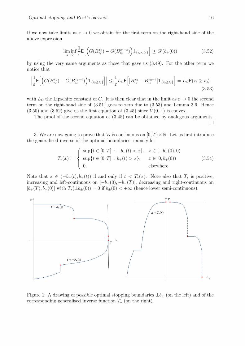
3. We are now going to prove that Vt is continuous on [0, T )×R. Let us first introducethe generalised inverse of the optimal boundaries, namely let

T∗(x) :=

supt ∈ [0, T ] : −b−(t) < x, x ∈ (−b−(0), 0)

supt ∈ [0, T ] : b+(t) > x, x ∈ [0, b+(0))

0, elsewhere

(3.54)

Note that x ∈ (−b−(t), b+(t)) if and only if t < T∗(x). Note also that T∗ is positive,increasing and left-continuous on [−b−(0),−b−(T )], decreasing and right-continuous on[b+(T ), b+(0)] with T∗(±b±(0)) = 0 if b±(0) < +∞ (hence lower semi-continuous).

Figure 1: A drawing of possible optimal stopping boundaries ±b± (on the left) and of thecorresponding generalised inverse function T∗ (on the right).


Lemma 3.10. Let h > 0 be as in Proposition 3.9 and for h ∈ (0, h) define the measureon R

σh(dy) :=V (T, y)− V (T − h, y)

hdy. (3.55)

Then the family (σh)h∈(0,h) is a family of negative measures such that

σh(dy)→ −ν(dy) weakly as h→ 0 (3.56)

and |σh(R)| ≤ C for all h ∈ (0, h) and suitable C > 0.

Proof. Let A ⊂ R be open bounded interval such that [−b−(T −h), b+(T −h)] ⊂ A. Notethat suppσh ⊂ A for all h ∈ (0, h) so that it is sufficient to study convergence of (σh)h>0

only on A. Take an arbitrary f ∈ C2b (R), then thanks to (3.54) we obtain∫

Rf(y)

V (T, y)− V (T − h, y)

hdy (3.57)

=

∫A

f(y)V (T, y)− V (T − h, y)

hdy

=

∫A

f(y)V (T, y)− V

(T∗(y) ∨ (T − h), y

)h

dy

+

∫A

f(y)V(T∗(y) ∨ (T − h), y

)− V (T − h, y)

hdy

=

∫A

f(y)V(T∗(y) ∨ (T − h), y

)− V (T − h, y)

hdy

where we have used that V(T∗(y) ∨ (T − h), y

)= G(y) = V (T, y). We now recall that Vt

is continuous in CT and Vt = −12Vxx in CT . Then we use Fubini’s theorem, integration by

parts and (3.43) to obtain2∫A

f(y)V(T∗(y) ∨ (T − h), y

)− V (T − h, y)

hdy (3.58)

=1

h

∫A

f(y)

∫ T∗(y)∨(T−h)

T−hVt(s, y)ds dy = − 1

2h

∫ T

T−h

∫ b+(s)

−b−(s)f(y)Vxx(s, y)dy ds

=− 1

2h

∫ T

T−h

[(fG′ − f ′G

∣∣b+(s)

−b−(s)+

∫ b+(s)

−b−(s)f ′′(y)V (s, y)dy

]ds.

We are interested in the limit of the above expression as h→ 0. It is useful to observethat since µ(±b±) = 0 we obtain

lims→T

12fG′

∣∣b+(s)

−b−(s)= lim

s→T

[f(b+(s))

(1− Fµ(b+(s))

)− f(−b−(s))

(− Fµ(−b−(s))

)](3.59)

=f(b+)(1− Fµ(b+)) + f(−b−)Fµ(−b−)

=12

[(fG′)((b+) +)− (fG′)((−b−)−)

]2Note that V (T, y)−V (t, y) = limε→0

(V (T−ε, y)−V (t, y)

)= limε→0

∫ T−εt

Vt(s, y)ds =:∫ T

tVt(s, y)ds,

hence the integral is well defined.


where we have also used b±(t) ↓ b±(T−) = b± as t ↑ T and Fν((b+) +) = 1, Fν((−b−)−) =0. We take limits in (3.58) as h → 0, use (3.59) and undo the integration by parts toobtain

limh→0

∫Rf(y)σh(dy) =− 1

2

[(fG′)((b+) +)− (fG′)

((−b−) −

)(3.60)

− (f ′G)(b+) + (f ′G)(−b) +

∫ b+(T )

−b−(T )f ′′(y)G(y)dy

]

=− 1

2

∫R1[−b−,b+]f(y)G′′(dy) = −

∫Rf(y)ν(dy).

The last equality above follows by supp ν ⊆ [−b−, b+]. To show that σh is finite on R it isenough to take f ≡ 1 in the above calculations and note that

σh(R) =− 1

2h

∫ T

T−h

(G′(b+(s))−G′(−b−(s))

)ds for all h ∈ (0, h). (3.61)

From the last expression it also immediately follows that

limh→0

σh(R) = −1

2

[G′((b+) +)−G′

((−b−) −

)]= −ν(R) = −1. (3.62)

In (3.60) we have not proven weak convergence of σh to −ν yet but this can now bedone easily. In fact any g ∈ Cb(R) can be approximated by a sequence (fk)k ⊂ C2

b (R)uniformly converging to g on any compact. In particular for any ε > 0 we can always findKε > 0 such that supA |fk − g| ≤ ε for all k ≥ Kε. Hence since supp ν ⊂ suppσh ⊂ A theprevious results give

limh→0

∣∣∣ ∫Rg(y)

(σh + ν)(dy)

∣∣∣ ≤ limh→0

ε(∣∣σh(R)

∣∣+ ν(R))

+ limh→0

∣∣∣ ∫Rfk(y)

(σh + ν)(dy)

∣∣∣ ≤ 2ε

(3.63)

for all k ≥ Kε. Since ε > 0 is arbitrary (3.56) holds.

Let us denote

p(t, x, s, y) :=1√

2π(s− t)e−

(x−y)22(s−t) , for t < s, x, y ∈ R (3.64)

the Brownian motion transition density. We can now give the main result of this section.

Proposition 3.11. It holds Vt ∈ C([0, T )× R).

Proof. Continuity of Vt holds separately inside CT and in DT , thus it remains to verify itacross the boundaries of CT . We only provide details for the regularity across the upperboundary as the ones for the lower boundary are completely analogous.

First we fix t ∈ (0, T ), denote x = b+(t) < +∞ and take a sequence (tn, xn)n∈N ⊂ CTsuch that (tn, xn) → (t, x) as n → ∞. For technical reasons that will be clear in whatfollows we assume t ≤ T−2δ for some arbitrarily small δ > 0 and with no loss of generality


we also consider tn < T − δ for all n. Now we aim at providing upper and lower boundsfor Vt(tn, xn) for each n ∈ N. A simple upper bound follows by observing that t 7→ V (t, x)is decreasing and clearly

Vt(tn, xn) ≤ 0 for all n ∈ N. (3.65)

For the lower bound we fix n and take h > 0 such that tn − h ≥ 0 and hence(tn − h, xn) ∈ CT . For simplicity we denote τn = τ∗(tn, xn) and τn,h := τ∗(tn − h, xn)as in (2.5) so that τn,h is optimal for the problem with value V (tn − h, xn). We use thesuperharmonic characterisation of V to obtain

V (tn, xn)− V (tn − h, xn) (3.66)

≥Exn[V (tn + τn,h ∧ (T − tn), Bτn,h∧(T−tn))− V (tn − h+ τn,h, Bτn,h)

]=Exn

[(V (tn + τn,h, Bτn,h)− V (tn − h+ τn,h, Bτn,h)

)1τn,h<T−tn

]+ Exn

[(V (T,BT−tn)− V (tn − h+ τn,h, Bτn,h)

)1τn,h≥T−tn

].

Observe that on the set τn,h < T − tn it holds V (tn − h + τn,h, Bτn,h) = G(Bτn,h) andV (tn + τn,h, Bτn,h) ≥ G(Bτn,h). On the other hand

Exn[V (tn − h+ τn,h, Bτn,h)

∣∣FT−tn] = V (T − h,BT−tn) on τn,h ≥ T − tn

by the martingale property of the value function inside the continuation region. Dividing(3.66) by h and taking iterated expectations it then follows

1

h

(V (tn, xn)− V (tn − h, xn)

)(3.67)

≥1

hExn

[(V (T,BT−tn)− V (T − h,BT−tn))1τn,h≥T−tn

]=Exn

[V (T,BT−tn)− V (T − h,BT−tn)

h

]− Exn

[1τn,h<T−tn

V (T,BT−tn)− V (T − h,BT−tn)

h

].

Since for all n we have δ ≤ T − tn then τn,h ≤ T − tn − δ ⊆ τn,h < T − tn andsince V (T,BT−tn)− V (T − h,BT−tn) ≤ 0 we obtain

−Exn[1τn,h<T−tn


h

](3.68)

≥− Exn

[1τn,h≤T−tn−δ


h

]=− Exn

[1τn,h≤T−tn−δEBτn,h

(V (T,BT−tn−τn,h)− V (T − h,BT−tn−τn,h)

h

)]where the last expression follows by the strong Markov property. Recalling now (3.55)and (3.64), we obtain the following from (3.67) and (3.68)

V (tn, xn)− V (tn − h, xn)

h(3.69)

≥∫R

(p(0, xn, T − tn, y)− Exn

[1τn,h≤T−tn−δp(0, Bτn,h , T − tn − τn,h, y)

] )σh(dy)


For every n ∈ N and h > 0 the function

fn,h(y) := p(0, xn, T − tn, y)− Exn[1τn,h≤T−tn−δp(0, Bτn,h , T − tn − τn,h, y)

], y ∈ R

(3.70)

is bounded and continuous with |fn,h(y)| ≤ C for some constant independent of n andh (this is easily verified since T − tn − τn,h ≥ δ in the second term of (3.70)). RecallingCorollary 3.8 it is not hard to verify that for any (yh)h>0 ⊂ R such that yh → y ∈ R ash→ 0 it holds

limh→0

fn,h(yh) = fn(y) := p(0, xn, T − tn, y)− Exn[1τn<T−tn−δp(0, Bτn , T − tn − τn, y)

],

where we have used that 1τn,h≤r → 1τn<r as h → 0, for any r > 0, since τn,h ↓τn. Moreover, Lemma 3.10 implies that

(σh(dy)/σh(R)

)h∈(0,h) forms a weakly converging

family of probability measures. Therefore we can use a continuous mapping theorem asin [17, Ch. 4, Thm. 4.27] to take limits in (3.69) as h→ 0 and get

Vt(tn, xn) ≥ limh→0

∫Rfn,h(y)σh(dy) = −

∫Rfn(y)ν(dy). (3.71)

Finally we take limits as n→∞ in the last expression and we use dominated conver-gence, the fact that τn → 0 as n → ∞ (see Lemma 3.6) and the upper bound (3.65), toobtain

limn→∞

Vt(tn, xn) = 0.

Since the sequence (tn, xn) was arbitrary the above limit implies continuity of Vt at (t, x).We can now repeat the same arguments for the case when a jump occurs by taking

an arbitrary x ∈ (b+(t−), b+(t)). Hence continuity of Vt holds across the upper optimalboundary.

4. It is a remarkable fact that in this context continuity of the time derivative Vt holdsat all points of the boundary regardless of whether or not the smooth-fit condition (3.43)holds there. As a consequence of the above theorem and of (3.4) we also obtain

Corollary 3.12. For any ε > 0 it holds that Vx and Vxx are continuous on the closure ofCT ∩ t ≤ T − ε. In particular for any (t, x) ∈ ∂CT and any sequence (tn, xn)n∈N ⊂ CTsuch that (tn, xn)→ (t, x) as n→∞, it holds

limn→∞

Vxx(tn, xn) = 0. (3.72)

For future frequent use we also define

U(t, x) :=V (t, x)−G(x), (t, x) ∈ [0, T ]× R (3.73)

then U ∈ C([0, T ]× R) and (3.4)–(3.5) imply(Ut + 1

2Uxx)(t, x) = −(ν − µ)(dx), x ∈

(− b−(t), b+(t)

), t ∈ [0, T ) (3.74)

U(t, x) = 0, x ∈ (−∞,−b−(t)] ∪ [b+(t),∞), t ∈ [0, T ) (3.75)

U(T, x) = 0, x ∈ R (3.76)

where the first equation holds in the sense of distributions.We conclude the section with a technical lemma that will be useful in the rest of the

paper.


Lemma 3.13. For any f ∈ Cb(R) one has

limt↑T

∫Rf(x)Vt(t, x)dx = −

∫Rf(x)ν(dx) (3.77)

i.e. it holds Vt(t, x)dx→ −ν(dx) weakly as a measure in the limit as t ↑ T .

Proof. It is enough to prove the claim for f ∈ C2b (R) as density arguments as in the final

part of the proof of Lemma 3.10 allow us to extend the result to f ∈ Cb(R).We take h > 0 as in Proposition 3.9 and we let A ⊂ R be an open bounded interval

such that [−b−(T − h), b+(T − h)] ⊂ A. Note that for U as in (3.73) the smooth-fitcondition (3.43) reads

Ux(t,±b±(t)) = 0, for t ∈ (T − h, T ). (3.78)

Then for any f ∈ C2b (R), t ∈ (T − h, T ) we use Proposition 3.11 along with Ut = Vt,

(3.74), (3.75) and (3.78) to obtain∫A

f(y)Vt(t, y)dy =

∫ b+(t)

−b−(t)f(y)Ut(t, y)dy (3.79)

=−∫ b+(t)

−b−(t)f(y)

(12Uxx(t, y)dy + (ν − µ)(dy)

)=− 1

2

∫A

f ′′(y)U(t, y)dy −∫ b+(t)

−b−(t)f(y)(ν − µ)(dy).

Taking limits as t → T dominated convergence, (3.76) and the facts that b±(t) ↓ b± andµ(±b±) = 0 give

limt→T

∫A

f(y)Vt(t, x)dx =−∫[−b−,b+]

f(x)(ν − µ)(dx) = −∫[−b−,b+]

f(x)ν(dx) (3.80)

thus concluding the proof.

4 The Skorokhod embedding

In this section we will show that the optimal boundaries b± found in Theorem 2.1 arethe boundaries of the time reversed Rost’s barrier associated to µ. The proof hinges on ainteresting probabilistic representation of Vt.

Here we recall the discussion in part 3 of Section 2 and the notation introduced thereinand we let s− and s+ be the reversed boundaries from Definition 2.3. We denote theextension to [0,∞) of the time reversed versions of the continuation set (2.6) and thestopping set (2.7) by

C−∞ :=

(t, x) : t ∈ [0,∞), x ∈(− s−(t), s+(t)

), (4.1)

D−∞ :=

(t, x) : t ∈ [0,∞), x ∈(−∞,−s−(t)] ∪ [s+(t),+∞

). (4.2)


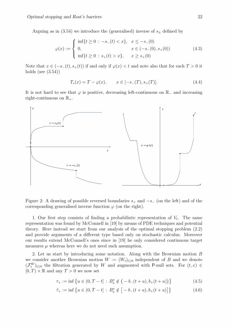
Arguing as in (3.54) we introduce the (generalised) inverse of s± defined by

ϕ(x) :=

inft ≥ 0 : −s−(t) < x, x ≤ −s−(0)

0, x ∈ (−s−(0), s+(0))

inft ≥ 0 : s+(t) > x, x ≥ s+(0)

(4.3)

Note that x ∈ (−s−(t), s+(t)) if and only if ϕ(x) < t and note also that for each T > 0 itholds (see (3.54))

T∗(x) = T − ϕ(x), x ∈ [−s−(T ), s+(T )]. (4.4)

It is not hard to see that ϕ is positive, decreasing left-continuous on R− and increasingright-continuous on R+.

Figure 2: A drawing of possible reversed boundaries s+ and −s− (on the left) and of thecorresponding generalised inverse function ϕ (on the right).

1. Our first step consists of finding a probabilistic representation of Vt. The samerepresentation was found by McConnell in [19] by means of PDE techniques and potentialtheory. Here instead we start from our analysis of the optimal stopping problem (2.2)and provide arguments of a different type based only on stochastic calculus. Moreoverour results extend McConnell’s ones since in [19] he only considered continuous targetmeasures µ whereas here we do not need such assumption.

2. Let us start by introducing some notation. Along with the Brownian motion Bwe consider another Brownian motion W := (Wt)t≥0 independent of B and we denote(FWt )t≥0 the filtration generated by W and augmented with P-null sets. For (t, x) ∈[0, T )× R and any T > 0 we now set

τ+ := infu ∈ (0, T − t] : Bx

u /∈(− b−(t+ u), b+(t+ u)

)(4.5)

τ+ := infu ∈ (0, T − t] : Bx

u /∈[− b−(t+ u), b+(t+ u)

](4.6)


τ− := infu > 0 : W x

u /∈(− s−(t+ u), s+(t+ u)

)(4.7)

τ− := infu > 0 : W x

u /∈[− s−(t+ u), s+(t+ u)

]. (4.8)

Both τ+ and τ+ are (Ft)-stopping times by right-continuity of the Brownian filtration. Itis important to observe that Lemma 3.6 and Corollary 3.7 imply that all boundary pointsof the set CT are regular for DT , i.e. the process started from (t, x) ∈ ∂CT immediatelyenters the interior of DT . As a consequence the following relations hold with τ∗ as in (2.5)

Pt,x(τ+ = 0) = 1 for all (t, x) ∈ ∂CTPt,x(τ∗ = τ+ = τ+) = 1 for all (t, x) ∈ [0, T )× R

Analogously τ− and τ− are (FWt )-stopping times. It seems non trivial to prove thatthe boundary of C−∞ is regular for D−∞ and therefore considering u > 0 in the definitionsof τ− and τ− is fundamentally different to considering u ≥ 0 (for more details regardingregular boundary points for Brownian motion one may read [18, Ch. 4.2] and referencestherein). However in [6] (see eq. (2.9) therein) one can find an elegant proof of the factthat3

Pt,x(τ− = τ−) = 1 for all (t, x) ∈ [0, T )× R. (4.9)

We remark that in what follows, and in particular for Lemma 4.1, we will find sometimesconvenient to use τ− instead of τ− to carry out our arguments of proof.

From now on we denote pC(t, x, s, y), s > t, the transition density associated withthe law Pt,x(Bs ∈ dy , s ≤ τ+) of the Brownian motion killed at τ+. Similarly we denotepC−(t, x, s, y), s > t, the transition density associated with the law Pt,x(Ws ∈ dy , s ≤ τ−)of W killed at τ−. It is well known that

pC(t, x, s, y) = p(t, x, s, y)− Et,x1s>τ+p(τ+, Bτ+ , s, y) (4.10)

for (t, x), (s, y) ∈ CT and

pC−(t, x, s, y) = p(t, x, s, y)− Et,x1s>τ−p(τ−,Wτ− , s, y) (4.11)

for (t, x), (s, y) ∈ C−∞ (see e.g. [17, Ch. 24]).The next lemma provides a result which can be seen as an extension of Hunt’s theorem

as given in [17, Ch. 24, Thm. 24.7] to time-space Brownian motion. Although such resultseems fairly standard we could not find a precise reference for its proof in the time-spacesetting and for the sake of completeness we provide it in the appendix.

Lemma 4.1. For all 0 ≤ t < s ≤ T and x ∈ (−b−(t), b+(t)), y ∈ (−b−(s), b+(s)), it holdspC(t, x, s, y) = pC−(T − s, y, T − t, x).

3. We can now use the above lemma to find an handy expression for Ut = Vt in terms ofpC−. Recall that the value function of the optimal stopping problem (2.2) may be denotedV T to account explicitly for the time horizon T > 0.

3To avoid confusion note that in [6] our functions s+ and −s− are denoted respectively b and c.


Proposition 4.2. Fix T > 0 and denote UT = V T − G = U as in (3.73). Then Ut ∈C([0, T )× R) and it solves(

(Ut)t + 12(Ut)xx

)(t, x) = 0, (t, x) ∈ CT (4.12)

Ut(t, x) = 0, (t, x) ∈ ∂CT ∩ t < T (4.13)

limt↑T

Ut(t, x)dx = −ν(dx), in the weak topology. (4.14)

Moreover the function Ut has the following representation

−Ut(t, x) =

∫RpC(t, x, T, y)ν(dy) =

∫RpC−(0, y, T − t, x)ν(dy), (t, x) ∈ [0, T )× R.

(4.15)

Proof. (a). We have already shown in Proposition 3.11 that Vt is continuous on [0, T )×Rand equals zero along the boundary of CT for t < T . Moreover Lemma 3.13 implies theterminal condition (4.14). In the interior of CT one has Vt ∈ C1,2 by standard results onCauchy-Dirichlet problems (see for instance [12, Ch. 3, Thm. 10]). It then follows that Utsolves (4.12) by differentiating (3.74) with respect to time.

(b). We now aim at showing (4.15). For (t, x) in the interior of DT the result is trivialsince Ut = 0 therein. Hence we prove it for (t, x) ∈ CT and the extension to ∂CT willfollow by continuity of Ut.

Let us recall τ+ = τ+ as in (4.5) and (4.6). In what follows we fix (t, x) ∈ CT and setτ+ = τ+(t, x). For ε > 0 we use Ito’s formula, (4.12)–(4.14), strong Markov property andthe definition of pC to obtain

−Ut(t, x) =− ExUt(t+ τ+ ∧ (T − t− ε), Bτ+∧(T−t−ε)) (4.16)

=− ExUt(T − ε, BT−t−ε)1τ+≥T−t−ε

=−∫RUt(T − ε, y)pC(t, x, T − ε, y)dy

Now we want to pass to the limit as ε→ 0 and use Lemma 3.13 and a continuous mappingtheorem to obtain (4.15). In order to do so we proceed in two steps.

(c.1). First we assume that b± > a±. Note that from (4.10) one can easily verify that(s, y) 7→ pC(t, x, s, y) is continuous at all points in the interior of CT by simple estimateson the Gaussian transition density. Therefore for any y ∈ [−a−, a+], any sequence (εj)j∈Nwith εj → 0 as j → ∞, and any sequence (yεj)j∈N converging to y as j → ∞ there isno restriction in assuming (T − εj, yεj) ∈ CT so that pC(t, x, T − εj, yεj) → pC(t, x, T, y)as j → ∞. Hence taking limits as ε → 0 and using (3.77) and a continuous mappingtheorem as in [17, Ch. 4, Thm. 4.27] we obtain

−Ut(t, x) =

∫RpC(t, x, T, y)ν(dy) =

∫RpC−(0, y, T − t, x)ν(dy) (4.17)

where the last equality follows from Lemma 4.1.

(c.2). Here we remove the assumption that b± > a±. Since µ(±b±) = 0 (see Assumption(D.3)) there is no loss of generality in assuming that Fµ ∈ C

([−b−− δ0, b+ + δ0]

)for some


δ0 > 0 sufficiently small. Then for arbitrary δ ∈ (0, δ0) we introduce the approximation

F δµ(x) :=

Fµ(x), x ∈ (−∞,−b− − δ]Fµ(−b− − δ), x ∈ (−b− − δ, b+ + δ)

Fµ(x)−(Fµ(b+ + δ)− Fµ(−b− − δ)

), x ∈ [b+ + δ,∞)

(4.18)

which is easily verified to fulfil

limδ→0

supx∈R

∣∣F δµ(x)− Fµ(x)

∣∣ = 0. (4.19)

Moreover for µδ(dx) := F δ(dx) we have

µδ(dx) =

µ(dx), x ∈ (−∞,−b− − δ] ∪ [b+ + δ,+∞)

0, x ∈ (−b− − δ, b+ + δ)(4.20)

Associated to each F δµ we consider an approximating optimal stopping problem with

value function V δ. The latter is defined as in (2.2) with G replaced by Gδ where Gδ

is simply defined as in (2.1) but with F δµ in place of Fµ. It is clear that the analysis

carried out in Theorem 3.2 and Proposition 3.9 for V and G can be repeated with trivialchanges when considering V δ and Gδ. Indeed the only conceptual difference betweenthe two problems is that F δ

µ does not describe a probability measure on R being in factµδ(R) < 1. In particular the continuation set for the approximating problem, i.e. theset where V δ > Gδ, is denoted by CδT and there exists two right-continuous, decreasing,

positive functions of time bδ± with bδ±(T−) = b± + δ such that

CδT :=

(t, x) ∈ [0, T )× R : x ∈(− bδ−(t), bδ+(t)

). (4.21)

It is clear from the definition of F δµ that for any Borel set A ∈ R it holds µδ(A) ≤ µδ

′(A)

if δ′ < δ. Hence for δ′ < δ, (t, x) ∈ [0, T )× R we obtain the following key inequality

V δ(t, x)−Gδ(x) = sup0≤τ≤T−t

Ex

∫RLzτ (ν − µδ)(dz) (4.22)

≥ sup0≤τ≤T−t

Ex

∫RLzτ (ν − µδ

′)(dz)

=V δ′(t, x)−Gδ′(x)

by Ito-Tanaka-Meyer formula. The above also holds if we replace V δ′ − Gδ′ by V − Gand it implies that the family of sets

(CδT)δ∈(0,δ0)

decreases as δ ↓ 0 with CδT ⊇ CT for all

δ ∈ (0, δ0). We claim that

limδ→0CδT = CT and lim

δ→0bδ±(t) = b±(t) for all t ∈ [0, T ). (4.23)

The proof of the above limits follows from standard arguments and is given in Appendixwhere it is also shown that

limδ→0

sup(t,x)∈[0,T )×K

∣∣V δ(t, x)− V (t, x)∣∣ = 0, K ⊂ R compact. (4.24)


Now for each δ ∈ (0, δ0) we can repeat the arguments that we have used above in thissection and in part 3 of Section 2 to construct a set Cδ,−∞ which is the analogue of the setC−∞. All we need to do for such construction is to replace the functions s+ and s− by theircounterparts sδ+ and sδ− which are obtained by pasting together the reversed boundaries

sδ,n± (t) := bδ,Tn± (Tn − t), t ∈ [0, Tn] (see Definition 2.3 and the discussion preceding it).As in (4.5)–(4.8) we define by τ δ+ the first time the process (Bt)t≥0 leaves [−bδ−(t), bδ+(t)],

t ∈ [0, T ] and by τ δ− the first strictly positive time the process (Wt)t≥0 leaves [−sδ−(t), sδ+(t)],t > 0. It is clear that τ δ− decreases as δ → 0 (since δ 7→ CδT is decreasing) and τ δ− ≥ τ−,P-a.s. for all δ ∈ (0, δ0). We show in appendix that in fact

limδ→0

τ δ− = τ−, P-a.s. (4.25)

The same arguments used to prove Proposition 3.11 can now be applied to show thatV δt is continuous on [0, T )×R as well and V δ

t = 0 outside of CδT ∩ t < T. Therefore, for

fixed δ ∈ (0, δ0), we can use the arguments of (a) and (b) above since b± + δ > a± andobtain

−U δt (t, x) =

∫RpC,δ(t, x, T, y)ν(dy) =

∫RpC,δ− (0, y, T − t, x)ν(dy) (4.26)

where obviously the transition densities pC,δ and pC,δ− have the same meaning of pC andpC− but with the sets CT and C−∞ replaced by CδT and Cδ,−∞ , respectively. Note that U δ

t ≤ 0,then for fixed t ∈ [0, T ) the expression above implies (see (4.10) and (4.11))

supx∈R

∣∣U δt (t, x)

∣∣ ≤ supx∈R

∫Rp(0, y, T − t, x)ν(dy) < +∞ for all δ ∈ (0, δ0)

and therefore there exists g ∈ L∞(R) such that U δt (t, · ) converges along a subsequence to

g as δ → 0 in the weak* topology relative to L∞(R). Moreover since the limit is uniqueand (4.24) holds, it must also be g( · ) = Ut(t, · ).

Now, for an arbitrary Borel set B ⊆ [−s−(T − t), s+(T − t)], (4.26) gives

−∫B

U δt (t, x)dx =

∫RPy(WT−t ∈ B, T − t ≤ τ δ−)ν(dy). (4.27)

We take limits in the above equation as δ → 0 (up to selecting a subsequence), we usedominated convergence and (4.25) for the right-hand side, and weak* convergence of U δ

t

for the left-hand side, and obtain

−∫B

Ut(t, x)dx =

∫RPy(WT−t ∈ B, T − t ≤ τ−)ν(dy). (4.28)

Finally, since B is arbitrary we can conclude that (4.15) holds in general.

4. Now we are ready to prove the main result of this section, i.e. Theorem 2.4, whosestatement we recall for convenience.

Theorem 2.5 Let W ν := (W νt )t≥0 be a standard Brownian motion with initial distribution

ν and define

σ∗ := inft > 0 : W ν

t /∈(− s−(t), s+(t)

). (4.29)


Then it holds

Ef(W νσ∗)1σ∗<+∞ =

∫Rf(y)µ(dy), for all f ∈ Cb(R). (4.30)

Proof. Let f ∈ C2b (R), take an arbitrary time horizon T > 0 and denote UT = U as in

(3.73). Throughout the proof all Stieltjes integrals with respect to measures ν and µ onR are taken on open intervals, i.e.∫ b

a

. . . =

∫(a,b)

. . . for a < b.

From a straightforward application of Ito’s formula we obtain

Ef(W νσ∗∧T ) =

∫Rf(y)ν(dy) +

1

2E

∫ σ∗∧T

0

f ′′(W νu )du (4.31)

=

∫Rf(y)ν(dy) +

1

2

∫ T

0

E1u≤σ∗f′′(W ν

u )du

Notice that σ∗ = τ− = τ− (see (4.7)–(4.9)) up to an obvious change in the initial conditionfor W0 in the definitions of τ− and τ−. Recall the probabilistic representation (4.15) ofUt. Then we observe that for u > 0


u ) =

∫Rf ′′(y)

(∫RpC−(0, x, u, y)ν(dx)

)dy (4.32)

=−∫ s+(u)

−s−(u)Ut(T − u, y)f ′′(y)dy

by (4.13). An application of Fubini’s theorem and the fact that y ∈ (−s−(u), s+(u)) ⇐⇒u > ϕ(y) (see (4.3)) gives∫ T

0


u ) du =−∫ T

0

(∫R1y∈(−s−(u),s+(u))Ut(T − u, y)f ′′(y)dy

)du (4.33)

=−∫Rf ′′(y)

(∫ T

0

1ϕ(y)<uUt(T − u, y)du)dy

=

∫Rf ′′(y)

(U(0, y)− U(T − ϕ(y), y)

)dy

=

∫Rf ′′(y)U(0, y)dy

where in the last line we have also used that P := (T − ϕ(y), y) = (T∗(y), y) ∈ ∂CT andU |∂CT = 0 (see (3.75)). Hence from (4.31) and (4.33) we conclude

Ef(W νσ∗∧T ) =

∫Rf(y)ν(dy) +

1

2

∫ s+(T )

−s−(T )f ′′(y)U(0, y)dy. (4.34)


The left hand side of (4.34) has an alternative representation and in fact one has

Ef(W νσ∗∧T ) =E1T≤σ∗f(W ν

T ) + E1σ∗<Tf(W νσ∗)

=

∫ s+(T )

−s−(T )

(∫Rf(y)pC−(0, x, T, y)ν(dx)

)dy + E1σ∗<Tf(W ν

σ∗). (4.35)

By using (4.15) once more we obtain∫ s+(T )

−s−(T )

(∫Rf(y)pC−(0, x, T, y)ν(dx)

)dy = −

∫ s+(T )

−s−(T )f(y)Ut(0, y)dy (4.36)

=

∫ s+(T )

−s−(T )f(y)

(ν − µ

)(dy) +

1

2

∫ s+(T )

−s−(T )f(y)Uxx(0, y)dy

where the last expression follows from (3.74). Now we must notice that since s±(T ) =bT±(0), then Proposition 3.5 and Corollary 3.4 imply that

limT→∞

s±(T ) = b∞± ≥ µ± (4.37)

where we recall that µ± are the endpoints of suppµ (see Assumption (C)). Since T isarbitrary and µ(±µ±) = 0 (see Assumption (C)) with no loss of generality we mayassume that T is large enough so that G′ is continuous on (−∞,−s−(t) + ε) ∪ (s+(t) −ε,+∞) for suitable ε > 0 and all t ≥ T .

Therefore point 2 of Proposition 3.9 holds and in particular (3.45) is verified at s±(T ) =bT±(0). Now integrating by parts the last term on the right of (4.36), using smooth-fit,(3.75) and (3.76), we conclude

Ef(W νσ∗∧T ) =E1σ∗<Tf(W ν

σ∗)−∫ s+(T )

−s−(T )f(y)µ(dy) (4.38)

+

∫Rf(y)ν(dy) +

1

2

∫ s+(T )

−s−(T )f ′′(y)U(0, y)dy.

Direct comparison of (4.38) and (4.34) then gives

E1σ∗<Tf(W νσ∗) =

∫ s+(T )

−s−(T )f(y)µ(dy) (4.39)

and hence taking limits as T →∞ and using dominated convergence we get

E1σ∗<∞f(W νσ∗) =

∫ s+(∞)

−s−(∞)

f(y)µ(dy) =

∫Rf(y)µ(dy) (4.40)

where the limit on the right holds by (4.37).Since (4.40) holds for any f ∈ C2

b (R) we can extend to arbitrary continuous functionsby a simple density argument. For any f ∈ Cb(R) we consider an approximating sequence(fk)k∈N ⊂ C2

b (R) such that fk → f pointwise as k → ∞. For each fk the equation(4.40) holds, then taking limits as k → ∞ and using dominated convergence we obtain(4.30).


As corollaries of the above result we obtain interesting and non trivial regularityproperties for the free-boundaries of problem (2.2). These are fine properties which aredifficult to obtain in general via a direct probabilistic study of the optimal stoppingproblem. Namely we obtain: i) flat portions of either of the two boundaries may occur ifand only if µ has an atom at the corresponding point (i.e. Gt + 1

2Gxx has an atom); ii)

jumps of the boundaries may occur if and only if Fµ is flat on an interval. Note that thelatter condition corresponds to saying that Gt + 1

2Gxx = 0 on an interval is a necessary

and sufficient condition for a jump of the boundary (precisely of the size of the interval)and therefore it improves results in [9] where only necessity was proven. It should also benoticed that Cox and Peskir [6] proved i) and ii) constructively but did not discuss itsimplications for optimal stopping problems.

Corollary 4.3. Let x0 ∈ R be such that µ(x0) > 0 then

i) if x0 > 0 there exist 0 ≤ t1(x0) < t2(x0) < +∞ such that s+(t) = x0 for t ∈ (t1, t2],

ii) if x0 < 0 there exist 0 ≤ t1(x0) < t2(x0) < +∞ such that s−(t) = x0 for t ∈ (t1, t2].

On the other hand, let either s+ or s− be constant and equal to x0 ∈ R on an interval(t1, t2], then µ(x0) > 0.

Proof. We prove i) arguing by contradiction. First notice that if x0 > 0 and µ(x0) > 0,then the upper boundary must reach x0 for some t0 > 0 due to Theorem 2.4. Let usassume that s+(t0) = x0 for some t0 > 0 and let us assume that s+ is strictly increasingon (t0 − ε, t0 + ε) for some ε > 0. Then µ(x0) = P(W ν

σ∗ = x0) = P(W νt0

= s+(t0)) = 0,hence a contradiction.

To prove the final claim let us assume with no loss of generality s+(t) = x0 for t ∈(t1, t2], then µ(x0) = P(W ν

σ∗ = x0) = P(W νt = x0 for some t ∈ (t1, t2], σ∗ > t1) > 0.

Corollary 4.4. Let (a, b) ⊂ R be an open interval such that µ((a, b)) = 0 and for anyε > 0 it holds µ((a, b+ ε)) > 0, µ((a− ε, b)) > 0, i.e. a and b are endpoints of a flat partof Fµ.

1. If s+(t) = a for some t > 0 then s+(t+) = b;

2. If −s−(t) = b for some t > 0 then −s−(t+) = a.

Proof. It is sufficient to prove 1 since the argument is the same for 2. Let us assumes+(t+) < b, then by left-continuity of the boundaries s+ ∈ C((t, t′)) for some t′ > t suchthat s+(t′) ≤ b. With no loss of generality (see Corollary 4.3) we also assume s+ strictlymonotone on (t, t′) otherwise µ should have an atom on (s+(t), s+(t′)). We then reach acontradiction by observing that

µ((a, b)) ≥ µ((s+(t+), s+(t′)

))=P(W νσ∗ ∈

(s+(t+), s+(t′)

))≥P(

supt≤s≤t′

W νs ≥ s+(t′), σ∗ > t

)> 0.

For (a, b) as in the corollary above we note that (3.7) implies s+(t−) = a for somet > 0 whenever s+(∞) ≥ a, i.e. s+ approaches a continuously. Similarly (3.8) implies−s−(t−) = b for some t > 0 whenever −s−(∞) ≤ b.


A Appendix

Proof of Lemma 4.1. The proof is a generalisation of the proof of [17, Thm. 24.7] and itwill be sufficient to give it in the case with t = 0 and s = T . In particular it is enough toshow that for any A,B ∈ B(R) with A ⊂ (−b−(0), b+(0)) and B ⊂ (−s−(0), s+(0)) onehas ∫

A

Px(BT ∈ B , T ≤ τ+)dx =

∫B

Px(WT ∈ A , T ≤ τ−)dx. (A-1)

For the sake of this proof and with no loss of generality we can consider the canonicalspace Ω = C([0,∞)), F = B

(C([0,∞))

)and a single Brownian motion X = (Xt)t≥0

defined as the coordinate process Xt(ω) = ω(t) with its filtration (FXt )t≥0 augmentedwith the P-null sets, where, with a slight abuse of notation, here we denote P the Wienermeasure on (Ω,F). With this convention τ+ denotes the first exit time of (Xt)t≥0 from[−b−(t), b+(t)], t ∈ [0, T ] and τ− denotes the first (strictly positive) exit time of (Xt)t≥0from [−s−(t), s+(t)], t ≥ 0.

By regularity of ∂CT it is clear that

T ≤ τ+ =⋂

q∈[0,T ]∩Q

Xq ∈ [−b−(q), b+(q)]

. (A-2)

It is also straightforward to see that

T ≤ τ− ⊆⋂

q∈[0,T ]∩Q

Xq ∈ [−s−(q), s+(q)]

=: HT (A-3)

and for the reverse inclusion we argue by contradiction and assume that there existsω0 ∈ HT such that ω0 /∈ T ≤ τ−. Then there also exists q0 = q0(ω0) ∈ [0, T ), q0 /∈ Q,such that Xq0(ω0) /∈ [−s−(q0), s+(q0)]. Consider ω0 fixed, then with no loss of generalitywe assume Xq0 ≥ s+(q0) + δ for some δ = δ(ω0) > 0. Let (qn)n ⊂ Q be an increasingsequence, depending on ω0, such that qn < q0 for all n and qn ↑ q0 as n → ∞, then forall n sufficiently large we get Xqn ≥ s+(q0) by continuity of trajectories. Recall that s+is left-continuous, then: i) if s+ is strictly increasing on an interval (q0 − ε, q0) for someε > 0 we get a contradiction since Xqn > s+(qn) and hence ω0 /∈ HT ; ii) if s+ is constanton (q0 − ε, q0) for some ε > 0 we equally get a contradiction since flat portions of theboundary are regular for

[0, T ) × R

\ C−∞ and hence Xqn ≥ s+(q0) = s+(qn) implies

Xqn′> s+(qn′) for some n′ > n and such that qn′ < q0, hence ω0 /∈ HT .

For simplicity and without loss of generality we assume T ∈ Q. Now, having estab-lished that

T ≤ τ− =⋂

q∈[0,T ]∩Q

Xq ∈ [−s−(q), s+(q)]

(A-4)

we can consider a sequence (πn)n∈N of dyadic partitions of [0, T ] defined by πn := tn0 , tn1 , . . . tnnwhere tnk := k

2nT , k = 1, 2, . . . 2n and then

T ≤ τ+ = limn→∞

⋂q∈πn

Xq ∈ [−b−(q), b+(q)]

, (A-5)

T ≤ τ− = limn→∞

⋂q∈πn

Xq ∈ [−s−(q), s+(q)]

. (A-6)


We set hn = tnk+1 − tnk = T/2n and denote pnh(x, y) = 1√2πhn

exp− 12hn

(x − y)2. By usingmonotone convergence and Chapman-Kolmogorov equation we obtain∫

B

Px(XT ∈ A, T ≤ τ−)dx (A-7)

= limn→∞

∫B

Px(Xq ∈ [−s−(q), s+(q)] for all q ∈ πn, XT ∈ A)dx

= limn→∞

∫pnh(x0, x1)p

nh(x1, x2) . . . p

nh(x2n−1, x2n)dx0 dx1 . . . dx2n

where the last integral is taken with respect to x0 ∈ B, x2n ∈ A and xk ∈ [−s−(tnk), s+(tnk)]for k = 1, 2, . . . 2n − 1. We interchange order of integration, relabel variables x2n−k = ykfor k = 0, 1, 2, . . . 2n and use symmetry of the heat kernel along with the fact that s±(q) =b±(T − q) to conclude∫

B

Px(XT ∈ A, T ≤ τ−)dx (A-8)

= limn→∞

∫pnh(y0, y1)p

nh(y1, y2) . . . p

nh(y2n−1, y2n)dy0 dy1 . . . dy2n

= limn→∞

∫A

Px(Xq ∈ [−b−(q), b+(q)] for all q ∈ πn, XT ∈ B)dx

=

∫A

Px(XT ∈ B, T ≤ τ+)dx

(=

∫A

Px(XT ∈ B, T ≤ τ+)dx

).

Hence (A-1) follows and the generalisation to arbitrary t < s can be obtained with thesame arguments.

Additional proofs for Proposition 4.2. 1. We begin by proving (4.24). We denote ‖ · ‖∞the L∞(R) norm. By direct comparison we obtain

(V δ − V

)(t, x) ≤ sup

0≤τ≤T−tEx2

∫ Bτ

0

(Fµ − F δ

µ

)(z)dz (A-9)

=2∥∥Fµ − F δ

µ

∥∥∞ sup

0≤τ≤T−tEx∣∣Bτ

∣∣and the same bound can be found for (V − V δ)(t, x). Then by an application of Jenseninequality and using that Ex(Bτ )

2 = x2 + E0B2τ = x2 + E0τ we get

∣∣V δ − V∣∣(t, x) ≤ 2

∥∥Fµ − F δµ

∥∥∞ sup

0≤τ≤T−t

(Ex∣∣Bτ

∣∣2)12 ≤ 2(|x|+

√T )∥∥Fµ − F δ

µ

∥∥∞. (A-10)

The latter goes to zero as δ → 0 by (4.19), uniformly for t ∈ [0, T ] and x in a compact.

2. Here we prove the claim in (4.23). It is sufficient to show that bδ+(t) ↓ b+(t) for allt ∈ [0, T ) since the proof for b− is analogous and the set convergence easily follows fromthe same arguments. Note that for each t the limit b0+(t) := limδ→0 b

δ+(t) exists and

b0+(t) ≥ b+(t) since δ 7→ bδ+(t) decreases as δ → 0 and bδ+(t) ≥ b+(t) for all δ ∈ (0, δ0).Let us assume that there exists t ∈ [0, T ) such that b0+(t) > b+(t). Pick x ∈ (b+(t), b0+(t)),


then by definition of bδ+ it should follow that infδ∈(0,δ0) Vδ(t, x)−Gδ(x) ≥ η > 0 for some

η = η(t, x). However this is clearly impossible by point 1 above.

3. To prove (4.25) we denote τ0 := limδ→0 τδ−, P-a.s. (the limit exists since the sequence

is monotone by point 2 above). Note that τ0 ≥ τ− and let us now prove that the reverseinequality also holds. With no loss of generality we consider the case when the process(t,W x

t ) starts at time zero with W x0 = x ∈ [−a−, a+]. Fix ω ∈ Ω, then if τ−(ω) = +∞

the claim is obvious. Let us assume that τ−(ω) < +∞ and with no loss of generalitylet us also assume W x

τ− ≥ s+(τ−). By definition of τ− there exists a sequence (tn, εn)n∈N,depending on ω, with tn > τ−, εn > 0, (tn, εn)→ (τ−, 0) as n→∞ and such that

W xtn ≥ s+(tn) + εn, for all n. (A-11)

Fix an index n, then due to (4.23) and point 2 above there exists ∆n,ω > 0 depending onn and ω and such that sδ+(tn) ≤ s+(tn)+εn/2 for all δ < ∆n,ω. Using the latter inequalityand (A-11) we find W x

tn ≥ sδ+(tn) + εn/2 for all δ < ∆n,ω and hence τ0 ≤ tn. Since tn maybe chosen arbitrarily close to τ− we conclude that τ0(ω) ≤ τ−(ω). By arbitrariness of ωthe (4.25) holds.

Acknowledgments: This work was funded by EPSRC grant EP/K00557X/1. I amgrateful to G. Peskir for showing me McConnell’s work and for many useful discussionsrelated to Skorokhod embedding problems and optimal stopping.

References

[1] Azema, J. and Yor, M. (1979). Une solution simple au probleme de Skorokhod.Seminaire de Probabilites, XIII, vol. 721, Lecture Notes in Math. pp. 90–115,Springer, Berlin.

[2] Blanchet, A., Dolbeault, J. and Monneau, R. (2006). On the continuity ofthe time derivative of the solution to the parabolic obstacle problem with variablecoefficients. J. Math. Pures Appl. 85 pp. 371–414.

[3] Chacon, R.M. (1985). Barrier stopping times and the filling scheme. PhD Thesis,Univ. of Washington.

[4] Cox, A.M.G., Hobson, D. and Ob loj, J. (2008). Pathwise inequalitiesfor local time: applications to Skorokhod embedding and optimal stopping.Ann. Appl. Probab. 18 (5) pp. 1870–1896.

[5] Cox, A.M.G., Ob loj, J. and Touzi, N. (2015). The Root solution to the multi-marginal embedding problem: an optimal stopping and time-reversal approach.Preprint to appear.

[6] Cox, A.M.G. and Peskir, G. (2013). Embedding Laws in Diffusions by Functionsof Time. To appear in Ann. Probab.

[7] Cox, A.M.G. and Wang, J. (2013). Root’s barrier: construction, optimality andapplications to variance options. Ann. Appl. Probab. 23 (3) pp. 859–894.


[8] Cox, A.M.G. and Wang, J. (2013). Optimal robust bounds for variance options.arXiv:1308.4363.

[9] De Angelis, T. (2015). A note on the continuity of free-boundaries in finite-horizonoptimal stopping problems for one dimensional diffusions. SIAM J. Control Optim. 53(1) pp. 167–184.

[10] De Angelis, T. (2015). Integral equations for Rost’s reversed barriers. ResearchReport No. 5, Probab. Statist. Group Manchester (to appear).

[11] De Angelis, T. and Peskir, G. (2015). Global C1 regularity of the value func-tion in optimal stopping problems. Research Report No. 6, Probab. Statist. GroupManchester (to appear).

[12] Friedman, A. (2008). Partial Differential Equations of Parabolic Type. Dover Pub-lications, New York.

[13] Galichon, A., Henry-Labordere, P. and Touzi, N. (2014). A stochastic con-trol approach to no-arbitrage bounds given marginals, with an application to look-back options. Ann. Appl. Probab. 24 (1) pp. 312–336.

[14] Gassiat, P., Oberhauser, H. and dos Reis, G. (2014). Root’s barrier, viscositysolutions of obstacle problems and reflected FBSDEs. arXiv : 1301.3798.

[15] Hobson, D. (2007). Optimal stopping of the maximum process: a converse to theresults of Peskir. Stochastics 79 (1-2) pp. 85–102.

[16] Hobson, D. (2011). The Skorokhod embedding problem and model independentbounds for option prices. Lecture Notes in Math. 2003, Springer pp. 267–318.

[17] Kallenberg, O. (2002). Foundations of modern probability (second edition).Springer-Verlag, New York.

[18] Karatzas, I. and Shreve, S. (1998). Brownian motion and stochastic calculus(second edition). Springer, New York.

[19] Mc Connell, T. R. (1991). The two-sided Stefan problem with a spatially depen-dent latent heat. Trans. Amer. Math. Soc. 326 pp. 669–699.

[20] Meilijson, I. (2003). The time to a given drawdown in Brownian motion. Seminairede Probabilites, XXXVII, vol. 1832, Lecture Notes in Math. pp. 94–108, Springer,Berlin.

[21] Ob loj, J. (2004). The Skorokhod embedding and its offspring. Probab. Surv. 1pp. 321–392.

[22] Ob loj, J. (2007). The maximality principle revisited: on certain optimal stoppingproblems. Seminaire de Probabilites, XL, vol. 1899, Lecture Notes in Math. pp. 309–328, Springer, Berlin.

[23] Peskir, G. (1999). Designing options given the risk: the optimal Skorokhod-embedding problem. Stochastic Process. Appl. 81 pp. 25–38.


[24] Peskir, G. and Shiryaev, A. (2006). Optimal Stopping and Free-Boundary Prob-lems. Lectures in Mathematics, ETH Zurich.

[25] Root, D.H. (1969). The existence of certain stopping times on Brownian motion.Ann. Math. Statist. 40 (2) pp. 715–718.

[26] Rost, H. (1971). The stopping distributions of a Markov Process. Invent. Math. 14pp. 1–16.

[27] Skorokhod, A.V. (1965). Studies in the theory of random processes. Addison-Wesley.

[28] Vallois, P. (1983). Le probleme de Skorokhod sur R: une approche avec le tempslocal. Seminaire de Probabilites, XVII, vol. 986, Lecture Notes in Math. pp. 227–239,Springer, Berlin.

Documents

Tiziano De Angelis - School of Mathematics · From optimal stopping boundaries to Rost’s reversed barriers and the Skorokhod embedding Tiziano De Angelis May 11, 2015 Abstract We