Título (usar minúsculas)

Lat. Am. J. Phys. Educ. Vol. 9, No. 1, March. 2015 1508-1 http://www.lajpe.org

Understanding the stationary and transient state of a solar array: Model and simulation

Carlos D. Rodríguez Gallegos1, Manuel S. Alvarez Alvarado

2

1Institut für Energiewandlung und Energiespeicherung, Universität Ulm, Helmholtzstraße

18, 89081 Ulm, Germany. 2Department of Electrical and Computer Engineering, New Jersey Institute of Technology

University Heights Newark, 07102 New Jersey, United States of America.

E-mail: [email protected]

(Received 22 October 2014, accepted 19 February 2015)

Abstract

The simulation of a solar array behavior is shown in this paper. In order to do this we first provide an overview of the

physical processes that occur in a solar cell for the photovoltaic effect to take place, its equivalent electrical circuit is

determined with an explanation of its components (photovoltaic current, diode, series and parallel resistance,

capacitance). The next step involves the design of the mathematical model of a solar array, this one will be simulated in

Simulink (from MATLAB) and the data we can obtain from it (currents, voltages, fill factor, power, efficiency, among

others) along with its comportment under different conditions (the I-V curves of series, parallel and combined solar

cells interconnections, the dependence with the intensity of the solar irradiance and the transient response considering

different technologies) will be shown and discussed. From this paper the reader will obtain a high level in order to

understand the operational principle of a solar array together with a practical notion of its electrical performance.

Keywords: Solar Array, Mathematical Model, Simulation, Stationary and Transient State.

Resumen

La simulación del comportamiento de un panel solar se muestra en este documento. Con el fin de hacer esto, primero

mostramos una visión general de los procesos físicos que ocurren en una célula solar para que ocurra el efecto

fotovoltaico, su circuito eléctrico equivalente se determina con una explicación de sus componentes (corriente

fotovoltaica, diodos, series y resistencias en paralelo, capacitancia). El siguiente paso consiste en el diseño del modelo

matemático de un panel solar, éste se simulará en Simulink (de MATLAB). Se muestran y discuten los datos que se

puedan obtener (corrientes, tensiones, factor de llenado, energía, eficiencia, entre otros) de su comportamiento en

diferentes condiciones (las curvas IV de la serie, las interconexiones paralelas y combinadas de las células solares, la

dependencia con la intensidad de la radiación solar, y la respuesta transitoria considerando diferentes tecnologías). Con

este artículo, el lector obtendrá un alto nivel de entendimiento del principio de funcionamiento de un panel solar,

además de una noción práctica de su rendimiento eléctrico.

Palabras clave: Matriz solar, Modelo matemático, Simulación, Estado estacionario y transitorio.

PACS: 88.40.jm, 88.40.jp, 07.05Qq. ISSN 1870-9095

I. INTRODUCTION

In our society, the amount of people is increasing in time,

because of this we require more industries, houses and

transport systems and as a result, a higher demand of

electrical energy is needed [1], mostly of this demand is

covered by means of non-renewable energy, nevertheless

this has a limit and we might reach a moment in the future

in which we would not be able to count with it; here comes

the need of focus in the research and develop of different

renewable energy systems [2].

Photovoltaic appears as a very popular way to generate

energy with a big potential to have a high development in

the future [3] because of the advantages it presents like for

example, it converts directly the energy from the light into

electricity, it doesn’t require any mechanical movement

(like the eolic generators or in hydro plants) so there will

not be losses due to friction, depending of our requirements

we can have portable solar cells like in our bags or a small

solar system in the roof of a home to provide energy to a

house, or even a big one that could extend to kilometers to

provide energy to a town (known as solar farms), due to this

the solar cell production is increasing in time [4].

On this paper we describe how to get the mathematical

model of a solar array considering different parameters of

this system and then we will proceed to develop the

simulation of this model in Simulink and explain the

obtained results.

Carlos D. Rodríguez Gallego et al.

Lat. Am. J. Phys. Educ. Vol. 9, No. 1, March 2015 1508-2 http://www.lajpe.org

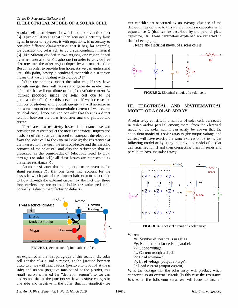
II. ELECTRICAL MODEL OF A SOLAR CELL

A solar cell is an element in which the photovoltaic effect

[5] is present; it means that it can generate electricity from

light. In order to represent it with equations, is necessary to

consider different characteristics that it has, for example,

we consider the solar cell to be a semiconductor material

[6] (like Silicon) divided in two regions, one region doped

by an n-material (like Phosphorous) in order to provide free

electrons and the other region doped by a p-material (like

Boron) in order to provide free holes. As we can understand

until this point, having a semiconductor with a p-n region

means that we are dealing with a diode D [7].

When the photons impact the solar cell, if they have

enough energy, they will release and generate an electron-

hole pair that will contribute to the photovoltaic current Iph

(current produced inside the solar cell due to the

photovoltaic effect), so this means that if we increase the

number of photons with enough energy we will increase in

the same proportion the photovoltaic current (if we assume

an ideal case), hence we can consider that there is a direct

relation between the solar irradiance and the photovoltaic

current.

There are also resistivity losses, for instance we can

consider the resistances at the metallic contacts (fingers and

busbars) of the solar cell needed to transport the electrons

from the solar cell to the external circuit; the resistances at

the intersection between the semiconductor and the metallic

contacts of the solar cell and also the resistances that are

presented in the semiconductor (electrons need to flow

through the solar cell); all these losses are represented as

the series resistance Rs.

Another resistance that is important to represent is the

shunt resistance Rp, this one takes into account for the

losses in which part of the photovoltaic current is not able

to flow through the external circuit, by the fact that those

free carriers are recombined inside the solar cell (this

normally is due to manufacturing defects).

FIGURE 1. Schematic of photovoltaic effect.

As explained in the first paragraph of this section, the solar

cell consist of a p and n region, at the junction between

these two, we will find cations (positive ions found at the n

side) and anions (negative ions found at the p side), this

small region is named the “depletion region”, so we can

understand that at the junction we have positive charges in

one side and negative in the other, that for simplicity we

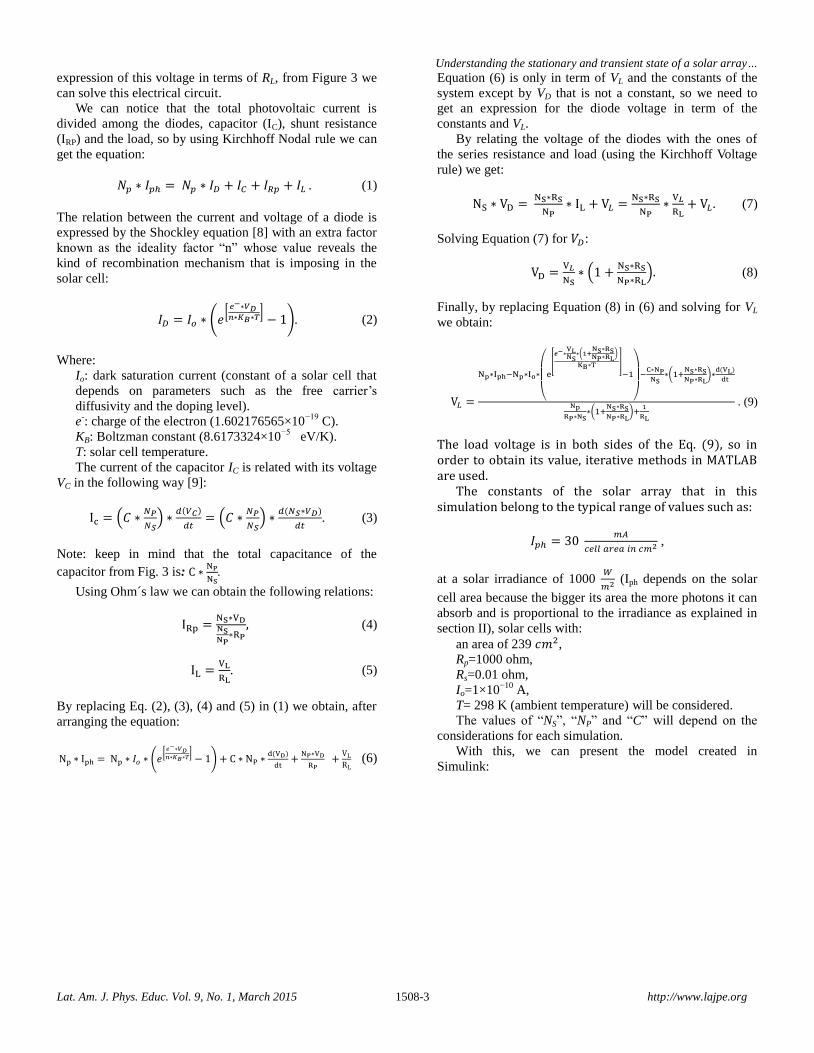
can consider are separated by an average distance of the

depletion region, due to this we are having a capacitor with

capacitance C (that can be described by the parallel plate

capacitor). All these parameters explained are reflected in

the following graph:

Hence, the electrical model of a solar cell is:

FIGURE 2. Electrical circuit of a solar cell.

III. ELECTRICAL AND MATHEMATICAL

MODEL OF A SOLAR ARRAY

A solar array consists in a number of solar cells connected

in series and/or parallel among them, from the electrical

model of the solar cell it can easily be shown that the

equivalent model of a solar array is (the output voltage and

current will have exactly the same expression by using the

following model or by using the previous model of a solar

cell from section II and then connecting them in series and

parallel to have the solar array):

FIGURE 3. Electrical circuit of a solar array.

Where:

Ns: Number of solar cells in series.

Np: Number of solar cells in parallel.

VD: Diode voltage.

ID : Current trough a diode.

RL: Load resistance.

VL: Load voltage (output voltage).

IL: Load current (output current).

VL is the voltage that the solar array will produce when

connected to an external circuit (in this case the resistance

RL), so in the following steps we will focus to find an

Understanding the stationary and transient state of a solar array…


expression of this voltage in terms of RL, from Figure 3 we

can solve this electrical circuit.

We can notice that the total photovoltaic current is

divided among the diodes, capacitor (IC), shunt resistance

(IRP) and the load, so by using Kirchhoff Nodal rule we can

get the equation:

. (1)

The relation between the current and voltage of a diode is

expressed by the Shockley equation [8] with an extra factor

known as the ideality factor “n” whose value reveals the

kind of recombination mechanism that is imposing in the

solar cell:

. (2)

Where:

Io: dark saturation current (constant of a solar cell that

depends on parameters such as the free carrier’s

diffusivity and the doping level).

e-: charge of the electron (1.602176565×10

−19 C).

KB: Boltzman constant (8.6173324×10−5

eV/K).

T: solar cell temperature.

The current of the capacitor IC is related with its voltage

VC in the following way [9]:

. (3)

Note: keep in mind that the total capacitance of the

capacitor from Fig. 3 is:

.

Using Ohm´s law we can obtain the following relations:

(4)

. (5)

By replacing Eq. (2), (3), (4) and (5) in (1) we obtain, after

arranging the equation:

(6)

Equation (6) is only in term of VL and the constants of the

system except by VD that is not a constant, so we need to

get an expression for the diode voltage in term of the

constants and VL.

By relating the voltage of the diodes with the ones of

the series resistance and load (using the Kirchhoff Voltage

rule) we get:

(7)

Solving Equation (7) for :

(8)

Finally, by replacing Equation (8) in (6) and solving for VL

we obtain:

. (9)

The load voltage is in both sides of the Eq. (9), so in order to obtain its value, iterative methods in MATLAB are used.

The constants of the solar array that in this simulation belong to the typical range of values such as:

,

at a solar irradiance of 1000

(Iph depends on the solar

cell area because the bigger its area the more photons it can

absorb and is proportional to the irradiance as explained in

section II), solar cells with:

an area of 239 ,

Rp=1000 ohm,

Rs=0.01 ohm,

Io=1×10−10

A,

T= 298 K (ambient temperature) will be considered.

The values of “NS”, “NP” and “C” will depend on the

considerations for each simulation.

With this, we can present the model created in

Simulink:



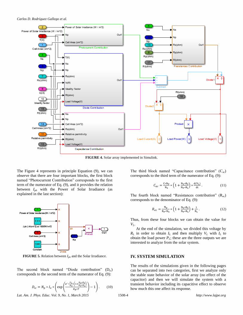
FIGURE 4. Solar array implemented in Simulink.

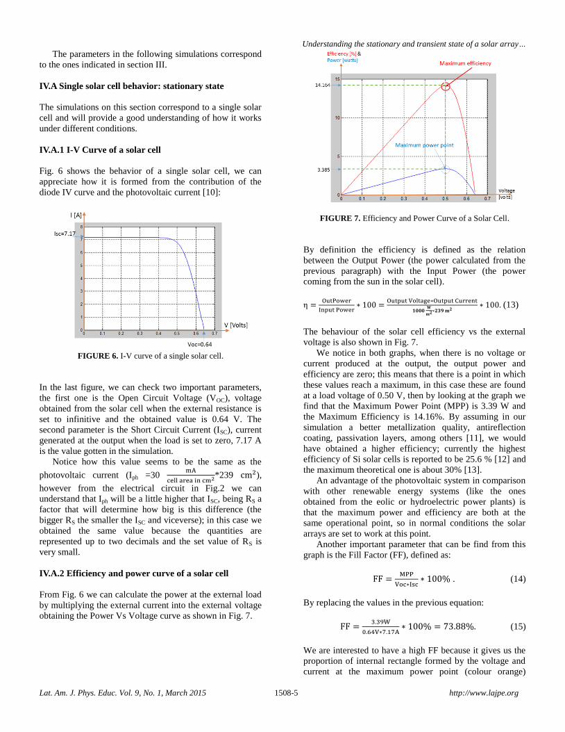
The Figure 4 represents in principle Equation (9), we can

observe that there are four important blocks, the first block

named “Photocurrent Contribution” corresponds to the first

term of the numerator of Eq. (9), and it provides the relation

between Iph with the Power of Solar Irradiance (as

explained in the last section):

FIGURE 5. Relation between Iph and the Solar Irradiance.

The second block named “Diode contribution” (Dic)

corresponds to the second term of the numerator of Eq. (9):

. (10)

The third block named “Capacitance contribution” (Cac)

corresponds to the third term of the numerator of Eq. (9):

. (11)

The fourth block named “Resistances contribution” (Rec)

corresponds to the denominator of Eq. (9):

. (12)

Thus, from these four blocks we can obtain the value for

VL.

At the end of the simulation, we divided this voltage by

RL in order to obtain IL and then multiply VL with IL to

obtain the load power PL; these are the three outputs we are

interested to analyze from the solar system.

IV. SYSTEM SIMULATION

The results of the simulations given in the following pages

can be separated into two categories, first we analyze only

the stable state behavior of the solar array (no effect of the

capacitor) and then we will simulate the system with a

transient behavior including its capacitive effect to observe

how much this one affect its response.



The parameters in the following simulations correspond

to the ones indicated in section III.

IV.A Single solar cell behavior: stationary state

The simulations on this section correspond to a single solar

cell and will provide a good understanding of how it works

under different conditions.

IV.A.1 I-V Curve of a solar cell

Fig. 6 shows the behavior of a single solar cell, we can

appreciate how it is formed from the contribution of the

diode IV curve and the photovoltaic current [10]:

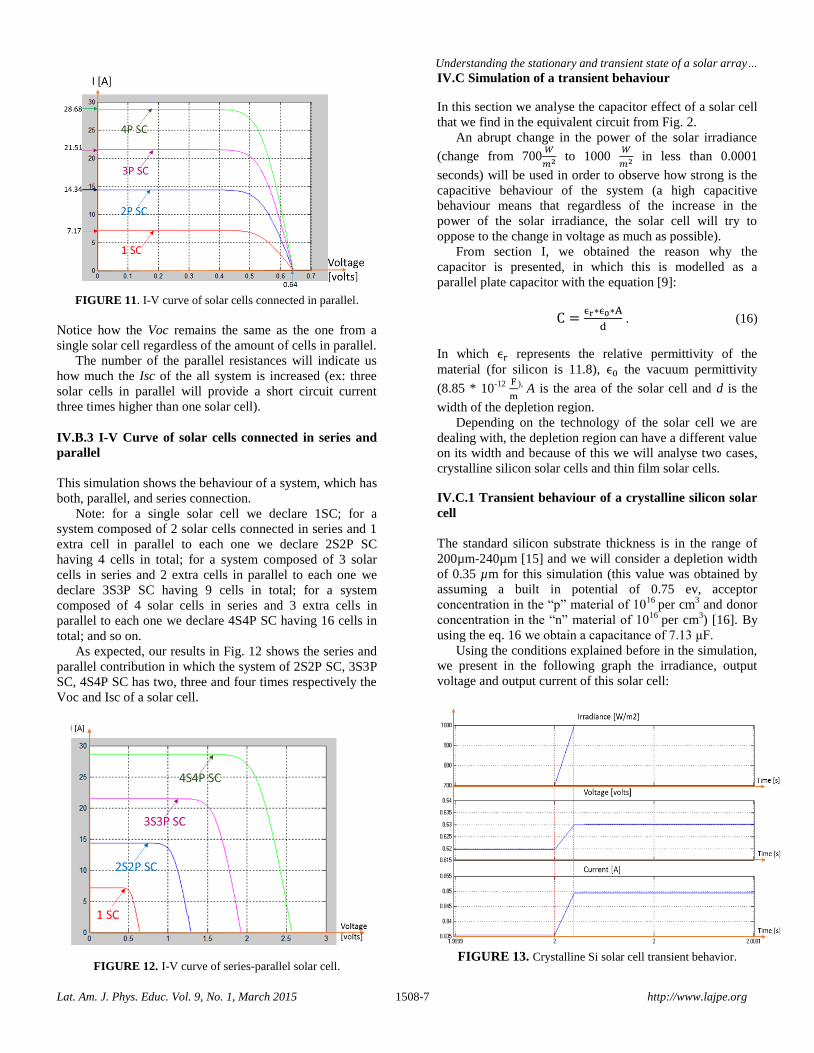
FIGURE 6. I-V curve of a single solar cell.

In the last figure, we can check two important parameters,

the first one is the Open Circuit Voltage (VOC), voltage

obtained from the solar cell when the external resistance is

set to infinitive and the obtained value is 0.64 V. The

second parameter is the Short Circuit Current (ISC), current

generated at the output when the load is set to zero, 7.17 A

is the value gotten in the simulation.

Notice how this value seems to be the same as the

photovoltaic current (Iph =30

*239 ),

however from the electrical circuit in Fig.2 we can

understand that Iph will be a little higher that ISC, being RS a

factor that will determine how big is this difference (the

bigger RS the smaller the ISC and viceverse); in this case we

obtained the same value because the quantities are

represented up to two decimals and the set value of RS is

very small.

IV.A.2 Efficiency and power curve of a solar cell

From Fig. 6 we can calculate the power at the external load

by multiplying the external current into the external voltage

obtaining the Power Vs Voltage curve as shown in Fig. 7.

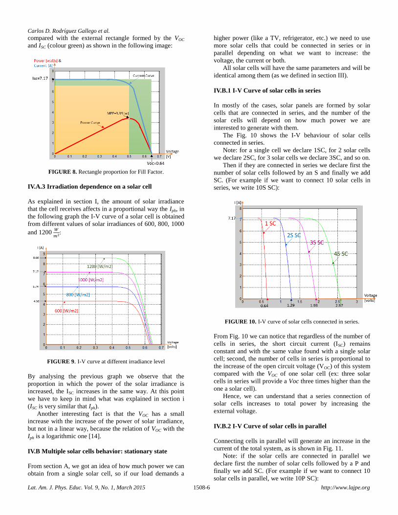
FIGURE 7. Efficiency and Power Curve of a Solar Cell.

By definition the efficiency is defined as the relation

between the Output Power (the power calculated from the

previous paragraph) with the Input Power (the power

coming from the sun in the solar cell).

(13)

The behaviour of the solar cell efficiency vs the external

voltage is also shown in Fig. 7.

We notice in both graphs, when there is no voltage or

current produced at the output, the output power and

efficiency are zero; this means that there is a point in which

these values reach a maximum, in this case these are found

at a load voltage of 0.50 V, then by looking at the graph we

find that the Maximum Power Point (MPP) is 3.39 W and

the Maximum Efficiency is 14.16%. By assuming in our

simulation a better metallization quality, antireflection

coating, passivation layers, among others [11], we would

have obtained a higher efficiency; currently the highest

efficiency of Si solar cells is reported to be 25.6 % [12] and

the maximum theoretical one is about 30% [13].

An advantage of the photovoltaic system in comparison

with other renewable energy systems (like the ones

obtained from the eolic or hydroelectric power plants) is

that the maximum power and efficiency are both at the

same operational point, so in normal conditions the solar

arrays are set to work at this point.

Another important parameter that can be find from this

graph is the Fill Factor (FF), defined as:

. (14)

By replacing the values in the previous equation:

(15)

We are interested to have a high FF because it gives us the

proportion of internal rectangle formed by the voltage and

current at the maximum power point (colour orange)



compared with the external rectangle formed by the VOC

and ISC (colour green) as shown in the following image:

FIGURE 8. Rectangle proportion for Fill Factor.

IV.A.3 Irradiation dependence on a solar cell

As explained in section I, the amount of solar irradiance

that the cell receives affects in a proportional way the Iph, in

the following graph the I-V curve of a solar cell is obtained

from different values of solar irradiances of 600, 800, 1000

and 1200

:

FIGURE 9. I-V curve at different irradiance level

By analysing the previous graph we observe that the

proportion in which the power of the solar irradiance is

increased, the ISC increases in the same way. At this point

we have to keep in mind what was explained in section i

(ISC is very similar that Iph).

Another interesting fact is that the VOC has a small

increase with the increase of the power of solar irradiance,

but not in a linear way, because the relation of VOC with the

Iph is a logarithmic one [14].

IV.B Multiple solar cells behavior: stationary state

From section A, we got an idea of how much power we can

obtain from a single solar cell, so if our load demands a

higher power (like a TV, refrigerator, etc.) we need to use

more solar cells that could be connected in series or in

parallel depending on what we want to increase: the

voltage, the current or both.

All solar cells will have the same parameters and will be

identical among them (as we defined in section III).

IV.B.1 I-V Curve of solar cells in series

In mostly of the cases, solar panels are formed by solar

cells that are connected in series, and the number of the

solar cells will depend on how much power we are

interested to generate with them.

The Fig. 10 shows the I-V behaviour of solar cells

connected in series.

Note: for a single cell we declare 1SC, for 2 solar cells

we declare 2SC, for 3 solar cells we declare 3SC, and so on.

Then if they are connected in series we declare first the

number of solar cells followed by an S and finally we add

SC. (For example if we want to connect 10 solar cells in

series, we write 10S SC):

FIGURE 10. I-V curve of solar cells connected in series.

From Fig. 10 we can notice that regardless of the number of

cells in series, the short circuit current (ISC) remains

constant and with the same value found with a single solar

cell; second, the number of cells in series is proportional to

the increase of the open circuit voltage (VOC) of this system

compared with the VOC of one solar cell (ex: three solar

cells in series will provide a Voc three times higher than the

one a solar cell).

Hence, we can understand that a series connection of

solar cells increases to total power by increasing the

external voltage.

IV.B.2 I-V Curve of solar cells in parallel

Connecting cells in parallel will generate an increase in the

current of the total system, as is shown in Fig. 11.

Note: if the solar cells are connected in parallel we

declare first the number of solar cells followed by a P and

finally we add SC. (For example if we want to connect 10

solar cells in parallel, we write 10P SC):



FIGURE 11. I-V curve of solar cells connected in parallel.

Notice how the Voc remains the same as the one from a

single solar cell regardless of the amount of cells in parallel.

The number of the parallel resistances will indicate us

how much the Isc of the all system is increased (ex: three

solar cells in parallel will provide a short circuit current

three times higher than one solar cell).

IV.B.3 I-V Curve of solar cells connected in series and

parallel

This simulation shows the behaviour of a system, which has

both, parallel, and series connection.

Note: for a single solar cell we declare 1SC; for a

system composed of 2 solar cells connected in series and 1

extra cell in parallel to each one we declare 2S2P SC

having 4 cells in total; for a system composed of 3 solar

cells in series and 2 extra cells in parallel to each one we

declare 3S3P SC having 9 cells in total; for a system

composed of 4 solar cells in series and 3 extra cells in

parallel to each one we declare 4S4P SC having 16 cells in

total; and so on.

As expected, our results in Fig. 12 shows the series and

parallel contribution in which the system of 2S2P SC, 3S3P

SC, 4S4P SC has two, three and four times respectively the

Voc and Isc of a solar cell.

FIGURE 12. I-V curve of series-parallel solar cell.

IV.C Simulation of a transient behaviour

In this section we analyse the capacitor effect of a solar cell

that we find in the equivalent circuit from Fig. 2.

An abrupt change in the power of the solar irradiance

(change from 700

to 1000

in less than 0.0001

seconds) will be used in order to observe how strong is the

capacitive behaviour of the system (a high capacitive

behaviour means that regardless of the increase in the

power of the solar irradiance, the solar cell will try to

oppose to the change in voltage as much as possible).

From section I, we obtained the reason why the

capacitor is presented, in which this is modelled as a

parallel plate capacitor with the equation [9]:

. (16)

In which represents the relative permittivity of the

material (for silicon is 11.8), the vacuum permittivity

(8.85 * 10-12

), A is the area of the solar cell and d is the

width of the depletion region.

Depending on the technology of the solar cell we are

dealing with, the depletion region can have a different value

on its width and because of this we will analyse two cases,

crystalline silicon solar cells and thin film solar cells.

IV.C.1 Transient behaviour of a crystalline silicon solar

cell

The standard silicon substrate thickness is in the range of

200µm-240µm [15] and we will consider a depletion width

of 0.35 µm for this simulation (this value was obtained by

assuming a built in potential of 0.75 ev, acceptor

concentration in the “p” material of 1016

per cm3 and donor

concentration in the “n” material of 1016

per cm3) [16]. By

using the eq. 16 we obtain a capacitance of 7.13 μF.

Using the conditions explained before in the simulation,

we present in the following graph the irradiance, output

voltage and output current of this solar cell:

FIGURE 13. Crystalline Si solar cell transient behavior.



From Fig. 13 we can observe that the capacitor of the solar

cell did not seem to oppose to the change in voltage

because when the power of the solar irradiance is changing

linearly, the voltage and the current were changing linearly

and the same relation when it was constant.

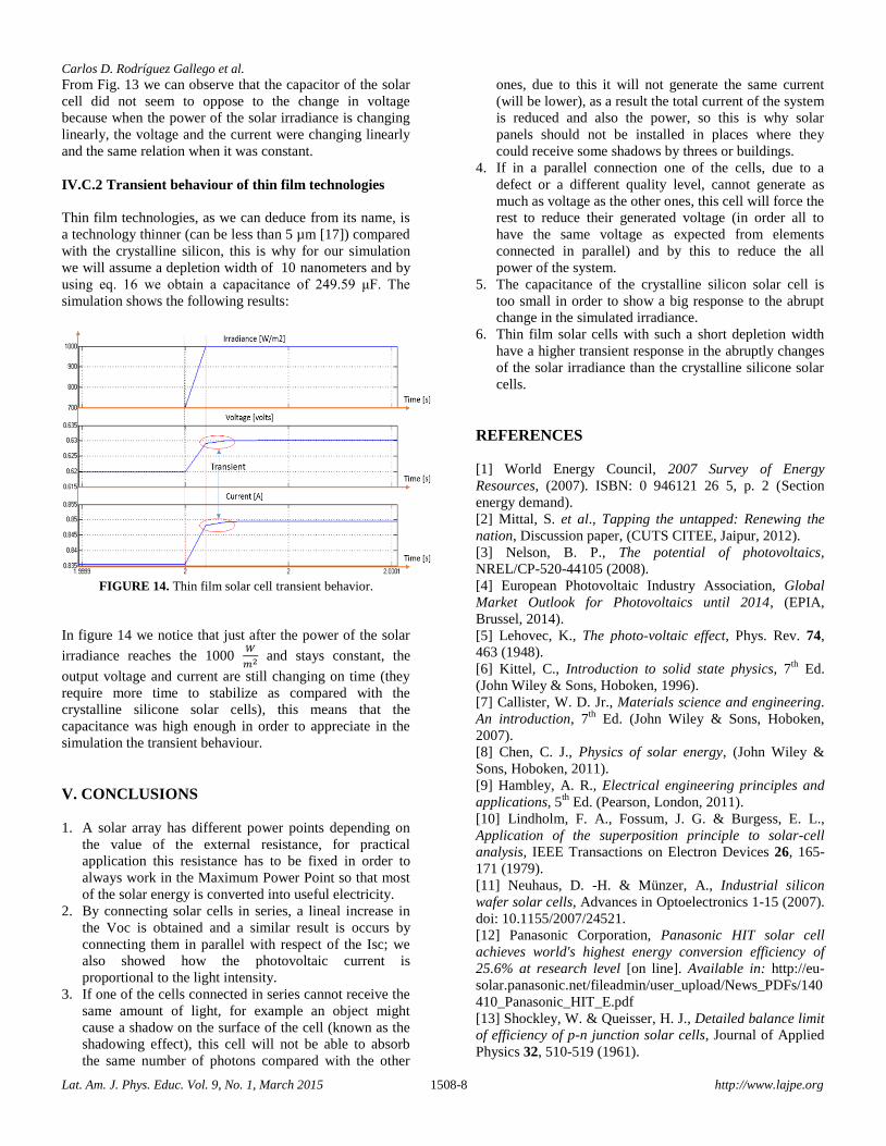
IV.C.2 Transient behaviour of thin film technologies

Thin film technologies, as we can deduce from its name, is

a technology thinner (can be less than 5 µm [17]) compared

with the crystalline silicon, this is why for our simulation

we will assume a depletion width of 10 nanometers and by

using eq. 16 we obtain a capacitance of 249.59 μF. The

simulation shows the following results:

FIGURE 14. Thin film solar cell transient behavior.

In figure 14 we notice that just after the power of the solar

irradiance reaches the 1000

and stays constant, the

output voltage and current are still changing on time (they

require more time to stabilize as compared with the

crystalline silicone solar cells), this means that the

capacitance was high enough in order to appreciate in the

simulation the transient behaviour.

V. CONCLUSIONS

1. A solar array has different power points depending on

the value of the external resistance, for practical

application this resistance has to be fixed in order to

always work in the Maximum Power Point so that most

of the solar energy is converted into useful electricity.

2. By connecting solar cells in series, a lineal increase in

the Voc is obtained and a similar result is occurs by

connecting them in parallel with respect of the Isc; we

also showed how the photovoltaic current is

proportional to the light intensity.

3. If one of the cells connected in series cannot receive the

same amount of light, for example an object might

cause a shadow on the surface of the cell (known as the

shadowing effect), this cell will not be able to absorb

the same number of photons compared with the other

ones, due to this it will not generate the same current

(will be lower), as a result the total current of the system

is reduced and also the power, so this is why solar

panels should not be installed in places where they

could receive some shadows by threes or buildings.

4. If in a parallel connection one of the cells, due to a

defect or a different quality level, cannot generate as

much as voltage as the other ones, this cell will force the

rest to reduce their generated voltage (in order all to

have the same voltage as expected from elements

connected in parallel) and by this to reduce the all

power of the system.

5. The capacitance of the crystalline silicon solar cell is

too small in order to show a big response to the abrupt

change in the simulated irradiance.

6. Thin film solar cells with such a short depletion width

have a higher transient response in the abruptly changes

of the solar irradiance than the crystalline silicone solar

cells.

REFERENCES

[1] World Energy Council, 2007 Survey of Energy

Resources, (2007). ISBN: 0 946121 26 5, p. 2 (Section

energy demand).

[2] Mittal, S. et al., Tapping the untapped: Renewing the

nation, Discussion paper, (CUTS CITEE, Jaipur, 2012).

[3] Nelson, B. P., The potential of photovoltaics,

NREL/CP-520-44105 (2008).

[4] European Photovoltaic Industry Association, Global

Market Outlook for Photovoltaics until 2014, (EPIA,

Brussel, 2014).

[5] Lehovec, K., The photo-voltaic effect, Phys. Rev. 74,

463 (1948).

[6] Kittel, C., Introduction to solid state physics, 7th

Ed.

(John Wiley & Sons, Hoboken, 1996).

[7] Callister, W. D. Jr., Materials science and engineering.

An introduction, 7th

Ed. (John Wiley & Sons, Hoboken,

2007).

[8] Chen, C. J., Physics of solar energy, (John Wiley &

Sons, Hoboken, 2011).

[9] Hambley, A. R., Electrical engineering principles and

applications, 5th

Ed. (Pearson, London, 2011).

[10] Lindholm, F. A., Fossum, J. G. & Burgess, E. L.,

Application of the superposition principle to solar-cell

analysis, IEEE Transactions on Electron Devices 26, 165-

171 (1979).

[11] Neuhaus, D. -H. & Münzer, A., Industrial silicon

wafer solar cells, Advances in Optoelectronics 1-15 (2007).

doi: 10.1155/2007/24521.

[12] Panasonic Corporation, Panasonic HIT solar cell

achieves world's highest energy conversion efficiency of

25.6% at research level [on line]. Available in: http://eu-

solar.panasonic.net/fileadmin/user_upload/News_PDFs/140

410_Panasonic_HIT_E.pdf

[13] Shockley, W. & Queisser, H. J., Detailed balance limit

of efficiency of p-n junction solar cells, Journal of Applied

Physics 32, 510-519 (1961).



[14] Markvart, T. & Castañer, L., Practical handbook of

photovoltaics fundamentals and applications (Elsevier,

London, 2003).

[15] Saga, T., Advances in crystalline silicon solar cell

technology for industrial mass production, NPG Asia

Materials 2, 96-102 (2010).

[16] Muhibbullah, M. et al., An equation of the width of the

depletion layer for a step heterojunction, Trans. Mat. Res.

Soc. Japan 37, 405-408 (2012).

[17] Saga, T., Advances in crystalline silicon solar cell

technology for industrial mass production, NPG Asia

Materials 2, 96-102 (2010).

Documents

Título (usar minúsculas)