Titre: Anomaly detection with the Switching Kalman Filter

Titre:Title:

Anomaly detection with the Switching Kalman Filter for structural health monitoring

Auteurs:Authors: Juong Ha Nguyen et James-A. Goulet

Date: 2018

Type: Article de revue / Journal article

Référence:Citation:

Nguyen, L. H. & Goulet, J.-A. (2018). Anomaly detection with the Switching Kalman Filter for structural health monitoring. Structural Control and Health Monitoring, 25(4), p. 1-18. doi:10.1002/stc.2136

Document en libre accès dans PolyPublieOpen Access document in PolyPublie

URL de PolyPublie:PolyPublie URL: https://publications.polymtl.ca/2868/

Version: Version finale avant publication / Accepted versionRévisé par les pairs / Refereed

Conditions d’utilisation:Terms of Use: Tous droits réservés / All rights reserved

Document publié chez l’éditeur officielDocument issued by the official publisher

Titre de la revue:Journal Title: Structural Control and Health Monitoring

Maison d’édition:Publisher: Wiley

URL officiel:Official URL: https://doi.org/10.1002/stc.2136

Mention légale:Legal notice:

This is the peer reviewed version of the following article: Nguyen, L. H. & Goulet, J.-A. (2018). Anomaly detection with the Switching Kalman Filter for structural health monitoring. Structural Control and Health Monitoring, 25(4), p. 1-18. doi:10.1002/stc.2136, which has been published in final form at https://doi.org/10.1002/stc.2136. This article may be used for non-commercial purposes in accordance with Wiley Terms and Conditions for Self-Archiving.

Ce fichier a été téléchargé à partir de PolyPublie, le dépôt institutionnel de Polytechnique Montréal

This file has been downloaded from PolyPublie, theinstitutional repository of Polytechnique Montréal

http://publications.polymtl.ca

https://publications.polymtl.ca/2868/

https://doi.org/10.1002/stc.2136

https://doi.org/10.1002/stc.2136

http://publications.polymtl.ca/

Anomaly Detection with the Switching Kalman

Filter for Structural Health Monitoring

Luong Ha Nguyen∗ and James-A. GouletDepartment of Civil, Geologic and Mining Engineering

Ecole Polytechnique de Montreal, CANADA

November 30, 2017

Abstract

Detecting changes in structural behaviour, i.e. anomalies over time is an importantaspect in structural safety analysis. The amount of data collected from civil structureskeeps expanding over years while there is a lack of data-interpretation methodologycapable of reliably detecting anomalies without being adversely affected by false alarms.This paper proposes an anomaly detection method that combines the existing BayesianDynamic Linear Models framework with the Switching Kalman Filter theory. Thepotential of the new method is illustrated on the displacement data recorded on a damin Canada. The results show that the approach succeeded in capturing the anomaliescaused by refection work without triggering any false alarms. It also provided thespecific information about the dam’s health and conditions. This anomaly detectionmethod offers an effective data-analysis tool for Structural Health Monitoring.

Keywords: Anomaly Detection, Bayesian, Dynamic Linear Models, Switch Kalman Filter, Struc-

tural Health Monitoring, False Alarm, Dam.

1 Introduction

Around the world, civil structures are in poor condition [1,2]. As early as in the 1970s manystructures have been monitored to improve the understanding of their behaviour [3,4]. Thisresearch field is known as Structural Health Monitoring (SHM). Quantities monitored on astructure are typically displacements, strains, inclination or accelerations [5, 6]. Sensingtechnology has evolved over the last decades and is now cheap and widely available. Thehardware developments led to an increase in the amount of available data. In this paper, wefocus on long-term condition SHM. Many methodologies from the field of applied statisticsand machine learning [7,8] have been proposed for interpreting the time-series data in orderto deduce valuable insights based on these data.

A first key aspect limiting the applicability of SHM is that there is currently a lackof data-interpretation methodology capable of reliably detecting anomalies in time serieswithout also being adversely affected by false alarms. An anomaly is defined here as a change

∗Corresponding author: [email protected]

1

NGUYEN and GOULET (2017). Anomaly Detection with the Switching Kalman Filter forStructural Health Monitoring. Preprint submitted to Structural Control and Heath Monitoring

in the behaviour of a structure. A second key aspect is that in order to be financially viablefor practical applications, data-interpretation methods must be easily transferable from onestructure to another and from one measurement type to another. This second aspect ismandatory if the objective is to deploy SHM systems across populations of structures. Athird key aspect is that no training sets with labeled conditions (normal and abnormal) areavailable.

Existing Regression Methods (RMs) for SHM model the dependence between observedstructural responses and time-dependent covariates such as temperature and loading. Inthe field of dam engineering, the most common regression method is the HST (Hydrostatic,Seasonal, Time) method [9–11] and analogue derivations [12–14] that have been applied tointerpret dam behaviour through displacement, pressure, and flow-rate data. In additionto the HST, Neural Network [15], Support Vector Machines [16, 17], Boosted RegressionTrees [18] and others [19,20] are used for the same purpose. The first drawback of theseRMs is that once the model is built using a training set, it stops evolving as new data iscollected. The second drawback is that anomaly detection is based on a hypothesis-testingprocedure. A probability density function of the error between observation and the modelprediction is identified for the training set and then employed to detect anomalies. Thepresence of the anomalies is tested based on the distance between the training set andtest-set confidence regions. This procedure tends to be prone to false alarms in the presenceof outliers.

Contrary to common RMs, State Space Models (SSMs) continue learning from thenew data after the training set. In the SSMs, the structural responses are modelled bythe superposition of hidden states that are not directly observed. An example for theSSMs is Autoregressive Models (ARs) that are employed to classify damage scenarios onexperimental data for the IASC–ASCE benchmark a four-storey frame structure, the Z24bridge in Switzerland and the Malaysia–Singapore Second Link bridge [21]. The ARs arealso applied to damage detection on the Steel-Quake structure at the Joint Research Centerin Ispra (Italy) [22]. The limited predictive capacity of ARs hinders their widespreadapplicability. Other dynamic modelling methods based on Kalman Filter variants [23,24]are used to identify changes in the modal parameters such as the stiffness and dampingfor detecting anomalies. Such as typically require detailed information about a structure,which is not suited for a widespread deployment across thousands of bridges and dams thatare all different from one to another.

Bayesian Dynamic Linear Models (BDLMs) [25] based on the SSMs have shown to be apromising solution in order to address the above limitations. The idea behind BDLM isthat the observed structural observation is decomposed into a set of hidden components.The generic hidden components can be among others, a Local Level to describe the baselineresponse of structures, a Periodic Component to describe periodic effects such as temperature,an Autoregressive Component to capture time-dependent model approximation errors. Inthe BDLM, the rate of changes in the evolution of the Local Level is characterized by aLocal Trend. If any changes occur in the Local Trend, a Local Acceleration componentmust be added to model its rate of change. The key challenge here is that in its currentform, the BDLM can only model behaviour of structures under stationary, i.e. normalconditions. In order to detect the occurrence of anomalies, it needs to be extended tooperate in non-stationary, i.e. abnormal, conditions.

2


This paper proposes an anomaly detection method that combines the existing BDLMwith the Switching Kalman Filter (SKF) theory [26]. In the field of machine learning, theSKF is used in many case studies [27–29] for handling non-stationary conditions. The keyfeatures of the approach proposed is that:

• It enables early anomaly detection

• It is robust towards false alarms in real operation condition

• It does not require labeled training data with normal and abnormal conditions.

The paper is organized as follows. The Section 2 presents a summary of the SKF theory.The Section 3 describes the methodology for anomaly detection. The section 4 illustratesthe potential of the new approach on displacement data recorded on a dam located inCanada.

2 Switching Kalman Filter

This section presents the mathematical formulations for the combination of existing BayesianDynamic Linear Model with the Switching Kalman Filter. A BDLM is defined by thefollowing linear equations:

Observation equation

yt = Ctxt + vt,

yt ∼ N (E[yt], cov[yt])

xt ∼ N (µt,Σt)

vt ∼ N (0,Rt)

(1)

Transition equation

xt = Atxt−1 + wt,{

wt ∼ N (0,Qt), (2)

where yt is the observation vector at the time t ∈ (1 : T ), Ct is the observation matrix, xt is the hidden state variables that they are not directly observed, vt is the Gaussianmeasurement error with mean zero and covariance matrix Rt, At is the transition matrix,and wt is the Gaussian model error with mean zero and covariance matrix Qt. Equations1 and 2 estimated using the Kalman Filter [30]. The specificity of BDLM is to buildmodel matrices At,Ct,Qt,Rt using a pre-defined sub-component structure [25]. The SKFenables to model the different states of a system, each having its own set of model matrixby estimating, over time steps, the probability of multiple model classes. Following thenotation from Murphy [26], the SKF algorithm is divided into the filter and collapse steps.

SKF-Filter step

The SKF-Filter step is equivalent to the Kalman filter employed for the existing BDLM.However, the notation for Kalman filter (KF) algorithm needs to be adapted to include theMarkov-switching variable st ∈ {1, 2, . . . , S}, each one corresponding to a distinct filtering

3


model defined by its model matrices. The Markov-switching variables at time t and t− 1are respectively st−1 = i and st = j. The superscript inside the parentheses i(j) is employedto denote the current state j at the time t given the state i at time t− 1. For the SKF, theprediction and measurement steps from the Kalman filter (KF) algorithm are rewritten as

KF-Prediction step

p(xi(j)t |y1:t−1

)= N

(xi(j)t ;µ

i(j)t|t−1,Σ

i(j)t|t−1

)Prior state estimate

µi(j)t|t−1 , A

i(j)t µit−1|t−1 Prior expected value

Σi(j)t|t−1 , A

i(j)t Σi

t−1|t−1

(Ai(j)t

)ᵀ+ Q

i(j)t Prior covariance

KF-Measurement step

p(xi(j)t |y1:t

)= N

(xi(j)t|t ;µ

i(j)t|t ,Σ

i(j)t|t

)Posterior state estimate

µi(j)t|t = µ

i(j)t|t−1 + K

i(j)t r

i(j)t Posterior expected value

Σi(j)t|t =

(I−K

i(j)t C

i(j)t

)Σi(j)t|t−1 Posterior covariance

ri(j)t , yt − y

i(j)t Innovation vector

yi(j)t , E[yt|y1:t−1] = C

i(j)t µ

i(j)t|t−1 Predicted observations vector

Ki(j)t , Σ

i(j)t|t−1

(Ci(j)t

)ᵀ (Gi(j)t

)−1Kalman gain matrix

Gi(j)t , C

i(j)t Σ

i(j)t|t−1

(Ci(j)t

)ᵀ+ R

i(j)t Innovation covariance matrix.

The Kalman gain matrix Ki(j)t represents the relative importance of the innovation vector

ri(j)t with regard to the prior expected value µ

i,(j)t|t−1 ≡ E[x

i(j)t |y1:t−1]. The model uncertainty

is described by the model error covariance matrix Qi(j)t which depends on the state i at

time t− 1 and the state j at time t. For the case where there is no state transition betweent− 1 and t, model classes are assumed to be dependent upon the arrival state j at time t

so that Qi(j)t = Qj

t . If between time steps t− 1 and t there is a transition from one state to

another, the matrix Qi(j)t needs to be identified i.e Q

i(j)t 6= Qj

t . For common cases, matricesdefining the transition and observation models are only dependent on the arrival state j attime t,

Ai(j)t = Aj

t , Ci(j)t = Cj

t , Ri(j)t = Rj

t .

The Kalman filter algorithm described above is summarized in its short form as

(µi(j)t|t ,Σ

i(j)t|t ,L

i(j)t ) = Filter(µjt−1|t−1,Σ

it−1|t−1,A

jt ,C

jt ,Q

i(j)t ,Rj

t ) (3)

4


where Li(j)t measures the likelihood that the state at time t− 1 was st−1 = i and that it

switches to st = j. The likelihood of such as switch Li(j)t is defined as

Li(j)t = p(yt|st = j, st−1 = i,y1:t−1)

= N (yt; Cjt µ

i(j)t|t−1, Rj

t + Σi(j)t|t−1).

Note that the Filter step presented in Equation 3 can either be performed using theKalman method as presented above or using the UD filter [25]. The UD method is equivalentto the Kalman method, yet it is numerically more stable [31].

SKF-Collapse step

The mean vector µjt|t ≡ E[xjt |y1:t] and covariance matrix Σjt|t ≡ cov[xjt |y1:t] are computed by

collapsing the outputs from the filtering models according to their previous state probability,likelihood and transition probabilities. In order to further describe the collapse step, weintroduce the notation

Pr(st−1 = i|y1:t−1) = πit−1|t−1 Previous state probability

Pr(st = j|st−1 = i) = Zi(j) Transition probability

Pr(st−1 = i, st = j|y1:t) = Mi(j)t−1,t|t Joint probability

Pr(st−1 = i|st = j,y1:t) = Wi(j)t−1|t State switching probability.

The joint probability of st = j and st−1 = i, given y1:t is evaluated as

Mi(j)t−1,t|t =

Li(j)t|t ·Z

i(j)·πit−1|t−1∑

i

∑j L

i(j)t|t ·Z

i(j)·πit−1|t−1

, (4)

The denominator of Equation 4 is a normalization constant ensuring that∑

i

∑j M

i(j)t−1,t|t =

1. The marginal probability of st = j is obtained through marginalization following

πjt|t =∑i

Mi(j)t−1,t|t. (5)

The collapsed mean vector µjt|t and covariance matrix Σjt|t are defined as a Gaussian mixture

so that

Wi(j)t−1|t =

Mi(j)t−1,t|t

πjt|t

µjt|t =∑i

µi(j)t|t ·W

i(j)t−1|t

m = µi(j)t|t − µjt|t

Σjt|t =

∑i

[W

i(j)t−1|t · (Σ

i(j)t|t + mmᵀ)

].

(6)

5


The short-form notation for the collapse step is

(µjt|t,Σjt|t, π

jt|t) = Collapse(µ

i(j)t|t ,Σ

i(j)t|t ,W

i(j)t−1|t).

An illustration of the SKF-filer and -collapse steps employed for describing the transitionbetween two possible models is presented in Figure 1. The goal is to evaluate the mean vector

Filter withmodel 1

Filter withmodel 2

Filter withmodel 1

Filter withmodel 2

µ1t−1|t−1

Σ1t−1|t−1

π1t−1|t−1

µ2t−1|t−1

Σ2t−1|t−1

π2t−1|t−1

µ1(1)t|t

Σ1(1)t|t

L1(1)t|t

µ1(2)t|t

Σ1(2)t|t

L1(2)t|t

µ2(1)t|t

Σ2(1)t|t

L2(1)t|t

µ2(2)t|t

Σ2(2)t|t

L2(2)t|t

Collapse

Collapse

µ1t|t

Σ1t|t

π1t|t

µ2t|t

Σ2t|t

π2t|t

time t− 1 time t

State 1

State 2

State 1

State 2

Figure 1: Illustration of the SKF algorithm for two states each having its own transitionmodel. (.) indicates the filtering model being used for computation.

µjt|t and the covariance matrix Σjt|t for each model, j ∈ {1, 2} along with the probability

πjt|t of each model at the time t, given the same two models at time t − 1. When goingfrom t− 1 to t, there are four possibilities of transitions from a starting state st−1 = i to an

arrival state st = j, each leading to its own mean vector µi(j)t|t , covariance matrix Σ

i(j)t|t and

likelihood Li(j)t|t . In the collapse step, the prior probability of each origin state is combinedwith the transition probability and the likelihood of each transition using Equation 4. Theend result of the collapse step is a mean vector, covariance matrix and a probability foreach model.

Combining the BDLM framework with SKF involves several unknown parameters thatneed to be learned from data. In common SHM applications, only structural responsesy1:t are available and the state of the structure st remains a hidden variable (i.e. non-observed). Therefore, the task of inferring st from y1:t can be categorized as semi-supervisedlearning [32]. In that context, the set of parameters P∗ is estimated employing the Maximum

6


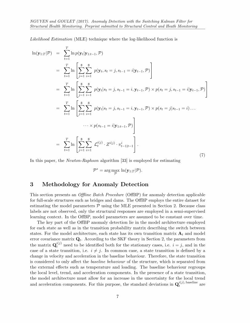
Likelihood Estimation (MLE) technique where the log-likelihood function is

ln(y1:T |P) =T∑t=1

ln p(yt|y1:t−1,P)

=T∑t=1

ln

S∑j=1

S∑i=1

p(yt, st = j, st−1 = i|yt−1,P)

=

T∑t=1

ln

S∑j=1

S∑i=1

p(yt|st = j, st−1 = i,yt−1,P)× p(st = j, st−1 = i|yt−1,P)

=

T∑t=1

ln

S∑j=1

S∑i=1

p(yt|st = j, st−1 = i,yt−1,P)× p(st = j|st−1 = i) . . .

· · · × p(st−1 = i|y1:t−1,P)

=

T∑t=1

ln

S∑j=1

S∑i=1

Li(j)t · Zi(j) · πit−1|t−1

.(7)

In this paper, the Newton-Raphson algorithm [33] is employed for estimating

P∗ = arg maxP

ln(y1:T |P).

3 Methodology for Anomaly Detection

This section presents an Offline Batch Procedure (OffBP) for anomaly detection applicablefor full-scale structures such as bridges and dams. The OffBP employs the entire dataset forestimating the model parameters P using the MLE presented in Section 2. Because classlabels are not observed, only the structural responses are employed in a semi-supervisedlearning context. In the OffBP, model parameters are assumed to be constant over time.

The key part of the OffBP anomaly detection lie in the model architecture employedfor each state as well as in the transition probability matrix describing the switch betweenstates. For the model architecture, each state has its own transition matrix At and modelerror covariance matrix Qt. According to the SKF theory in Section 2, the parameters from

the matrix Qi(j)t need to be identified both for the stationary cases, i.e. i = j, and in the

case of a state transition, i.e. i 6= j. In common case, a state transition is defined by achange in velocity and acceleration in the baseline behaviour. Therefore, the state transitionis considered to only affect the baseline behaviour of the structure, which is separated fromthe external effects such as temperature and loading. The baseline behaviour regroupsthe local level, trend, and acceleration components. In the presence of a state transition,the model architecture must allow for an increase in the uncertainty for the local trend

and acceleration components. For this purpose, the standard deviations in Qi(j), baselinet are

7


treated as an unknown parameter to be inferred from observations. An example for such asthis case will be illustrated in Section 4.2. The transition probability matrix Zt is identifiedbased on the number of states. For S states st ∈ {= 1, 2, 3 · · · , S}, the matrix Zt is definedas

Zt =

Z11 Z12 · · · Z1S

Z21 Z22 · · · Z2S

......

. . ....

ZS1 ZS2 · · · ZSS

where Zij = Pr(st = j|st−1 = i) with

∑Sj=1 Z

ij = 1.

The performance of the Newton-Raphson (NR) algorithm in Section 2 for learningparameters depends on (1) the initial parameter values P0 and (2) the initial mean µ0

and covariance Σ0 for the hidden states. The log-likelihood function is usually non-convex;poor guesses for either initial parameter values or hidden state initial values are prone tolead to a local maximum. In the case of anomaly detection, such a local maximum cantrigger false alarms. In order to overcome this limitation, random sets of initial parametervalues should be tested during the optimization procedure to ensure proper initial values.The second limitation is addressed using what we define as the multi-pass technique. Themulti-pass recursively employs the Switch Kalman Smoother (SKS) [26] for estimating µ0

and covariance Σ0 for hidden states. Figure 2 illustrates the utilization of the multi-pass inthe OffBP. During training, the model is first built using the initial parameter values Pn,

Pn D µ0,Σ0

Newton-Raphsonalgorithm

Pn+1,Ln+1

converged rem(n+ 1, N) = 0

SwitchingKalman Smoother

µnew0 ,Σnew

0 Lnew > Ln+1

P∗

no

yes

yes

yes

n = 0

no

n=n

+1

non = 0

Figure 2: Illustration of the offline batch procedure using the multi-pass. rem(n + 1, N)indicates the remainder after dividing N into n+ 1.

8


initial values for hidden states {µ0,Σ0}, and the training data D. The NR algorithm is thusemployed for estimating the model parameters Pn+1 and the corresponding log-likelihoodLn+1. After N iterations, µnew

0 and Σnew0 are estimated using SKS and the index n is reset

to 0. To be accepted as new initial values, the log-likelihood evaluated using {µnew0 ,Σnew

0 }needs to be greater than Ln+1. This procedure is repeated until the convergence criterionis reached. The final output of the procedure is the set of optimal parameters P∗. Forthe practical applications, N should be chosen so that the convergence criteria is not metbefore reaching N iterations. In common cases, N increases with the number of parametersto be estimated. In order to increase efficiency, the amount of data employed for estimatingthe initial values µnew

0 and Σnew0 can be smaller than the training data employed for the

parameter optimization procedure.

4 Case-Study

In this study, the approach proposed for anomaly detection is applied to the displacementdata collected on a dam located in Canada. The sensor studied is located on the westbank of the dam as shown in Figure 3. The displacement of the dam is monitored by an

Downstream

Dam displacement along the x-axis

West bank

ZX

Y

Uptream

East bank

Figure 3: Location plan of sensors deployed across the structure to monitor the dambehaviour.

inverted pendulum system that provides the measurements in three orthogonal directions.The X-direction points toward the West Bank, the Y-direction follows the water flow andthe Z-direction points upward.

4.1 Data Description

In order to examine the potential of the proposed anomaly detection method, this paperstudies the horizontal displacement data along the X-direction recorded over the periodof 13 years and 1 month (8364 time stamps) as shown in Figure 4. The observation errorstandard deviation σR = 0.3 mm was provided by the instrumentation engineers. Based

9


02-12 06-03 09-07 12-10 16-02−25.28

−13.25

−2.78

Time [YY-MM]

Disp

l,y t,

[mm

]

Figure 4: X-direction displacement data collected over the period of 13 years and 1 month.

on the raw data, one can observe a linear trend and a seasonal pattern with a period ofone year. The seasonal pattern reaches its maximum during winter and minimum duringsummer and is non-harmonic because of the lack of symmetry with respect to the horizontalaxis. The non-harmonic behaviour can be explained by the dependence of the displacementdata on the water temperature [14, 34], where its variation is not harmonic due to theunbalanced duration between the reservoir warming and cooling periods. Figure 5 presentsthe time-step length for the entire dataset. Time-step length varies in the range between

02-12 06-03 09-07 12-10 16-02100

101

102

103

Time [YY-MM]

Tim

est

epsiz

e[h

] = 36 days

= 24 hours= 12 hours

= 1 hour

Figure 5: Time-step size is presented in a log scale.

1 hour to 36 days in which the two most frequent time steps are 12 and 24 hours. Inorder to adapt with the non-uniformity of time steps, the parameters need to be defined asa function of the time-step length where the reference time-step is selected by the mostfrequent one [25].

4.2 Model Construction

The probability of a state switch is estimated for two model classes representing respectivelya state st ∈ {1 : Normal , 2 : Abnormal}. The set of components employed in each model

10


class is identical and follow

xt =

xLLt︸︷︷︸local level

, xLTt︸︷︷︸local trend

, xLAt︸︷︷︸local acceleration

, xT1,S1t , xT1,S2t︸︷︷︸cycle, p = 365.24 days

, xT2,S1t , xT2,S2t︸︷︷︸cycle, p = 182.62 days

, xARt︸︷︷︸AR

ᵀ

(8)

In order to differentiate models, the local acceleration component for the Normal modelclass is forced to be equal to zero at every time step. This is done by assigning a value ofzero to the line and row corresponding to the local acceleration component in the transitionmatrix At and model error covariance matrix Qt, see Appendix A for details. This constrainforces the Normal model class to have a constant velocity, i.e. acceleration = 0, while stillallowing the Abnormal model to have a non-zero acceleration. The baseline behaviour isdefined as the interaction of the local level, trend, and acceleration components. For bothmodels, a superposition of two hidden harmonic components with a period of 365.24 and182.62 days is used to describe the relationship between the displacement data and thehidden non-harmonic seasonal effect observed in the data, i.e. water temperature. Also,the AR component captures the time dependent model prediction errors.

The transition probability matrix is

Z =

[Z11 Z12

Z21 Z22

], (9)

where Zij = Pr(st = j|st−1 = i) with i, j = 1, 2 is the prior probability of transitioning froma state i at time t− 1 to a state j at time t. In order to be valid, this transition matrixmust satisfy

∑j Z

ij = 1. Given this constraint, only transition probabilities Zii need to bedefined as unknown parameters to be learned using MLE.

As presented in Section 3, the matrix Qt needs to be defined in the case where there isa state transition between the previous state i at time t− 1 and the arrival state j at timet. For this case-study, the local acceleration in the normal model is forced to be equal tozero so that only the uncertainty on the local trend component in the baseline behaviour isconsidered. In the case where there is no state transition from the state i to the state j,the model classes depend only on the arrival states j at time t. Therefore, the matricesQi(j),baseline are defined as

Q1(2), baselinet =

(σLA)2 · ∆t2

20 0 0

0 (σLTT)2 · ∆t3

3 0

0 0 (σLA)2 ·∆t

Q

2(2), baselinet = Q2, baseline

t

Q2(1), baselinet =

(σLT)2 · ∆t3

3 0 0

0 (σLTT)2 ·∆t 0

0 0 0

Q

1(1), baselinet = Q1, baseline

t

11


where σLA ∈ R+ is local acceleration standard deviation for abnormal model, σLT ∈ R+ islocal trend standard deviation for normal model, σLTT ∈ R+ is local-trend transition (LTT)standard deviation for the state transition models, and ∆t is the time step at time t. Thefull matrix Qt employed in this case-study is presented in Appendix A. In this case-study,we employ the UD method in the filter step presented in Equation 3.

4.3 Parameter Estimation

The convergence of the parameter optimization is reached when the log-likelihood betweentwo consecutive loops satisfies

‖log-likelihoodn − log-likelihoodn−1‖ ≤ 10−7 × ‖log-likelihoodn−1‖,

where n corresponds to nth optimization loop. The initial mean µ0 and covariance Σ0 forhidden states are estimated using the multi-pass presented in Section 3 using a period of5 years (1694 data points) and the number of iterations N = 30. This period is selectedbecause of the absence of the state switch which is causing numerical instabilities in theSwitching Kalman Smoother estimations. The set of unknown parameters P is defined asfollow

P ={Z11, Z22, φAR, σLT, σLA, σLTT, σT1, σT2, σAR

}, (10)

where the possible range for each parameter is: transition probabilities; Zii ∈ (0, 1),autocorrelation coefficient ; φAR ∈ (0, 1), local trend standard deviation; σLT ∈ R+, localacceleration standard deviation; σLA ∈ R+, transition local trend standard deviation; σLTT ∈R+, harmonic-component standard deviations for a period of 365.24 and 182.62 days;{σT1, σT2} ∈ R+ respectively, and autocorrelation standard deviation; σAR ∈ R+. Initialparameter values are estimated based on engineering heuristics so that

P0 ={

0.9999, 0.95, 0.986, 1.62× 10−8, 4× 10−4, 0.07, 5.1× 10−7, 2.7× 10−7, 0.03}.

This optimization procedure employs the entire dataset (8364 data points) for estimatingthe parameter values P∗.

4.4 Results and Discussion

The set of parameters P is estimated with MLE for the entire dataset. The parametercalibration is done on a computer with 32 Gb of Random Access Memory (RAM) and Inteli7 processor. The computational time required for the calibration task is approximately anhour and a half. The optimal parameter values identified are

P∗ = {1, 0.912, 0.996, 3.65× 10−6, 2× 10−8, 7.4× 10−4, 0.062, 1.9× 10−6, 2.78× 10−5, 0.021},

where the ordering of each parameter remains identical as in Equation 10. The log-likelihoodassociated with this set of parameters is ln p(y1:T |P∗) = 1784.3. Combining the BDLMframework with SKF serves two purposes: (1) it enables the detection of anomalies withouttriggering false alarms and (2) it decomposes the observations into their hidden components.Figure 6 presents the probabilities of each model class estimated at each time step. Themethod proposed identifies that there is an abnormal event occurring between July 8 and

12


02-12 06-03 09-07 12-10 16-020

0.5

1

Time [YY-MM]

Pr(

s)

Normal

Abnormal!2010-07-08

2010-07-11

2010-09-08

Figure 6: Probabilities of the two states are evaluated using SKF algorithm for the entiredataset.

11, 2010. This anomaly was caused by refection work that took place on the dam in earlyJuly. After the work was completed, the model identifies that the dam behaviour returnsto a normal behaviour. This example of application demonstrates how anomalies can bedetected without triggering any false alarm that would jeopardize the applicability of theapproach.

Figure 7 presents the hidden components estimated for the entire dataset. The solidblack line represents the mean values µ and its ±1σ standard deviation interval is representedby the shaded region. Figure 7a, b, and c show a sudden change in the local level, trendand acceleration at the moment when the anomaly occurred. These three figures showhow the baseline behaviour of the structure can be isolated from the effect of externalfactors. The external effect is modeled by a superposition of two harmonic components inFigure 7d and e. The local trend and local acceleration show a stable behaviour beforethe anomaly with estimated values of respectively −2.0 mm/year and −0.0054 mm/year2.During the abnormal event, local trend and acceleration components indicate a discontinuitybefore returning to a normal behaviour where the acceleration is zero. After the anomaly,it is estimated that the rate of change in the structure displacement has increased inmagnitude from −2.0 to −2.9 mm/year. Figure 7f shows that the autoregressive component,as expected, follows a stationary procedure. If it would not be the case, the non-stationarywould indicate that either the component choice, or the optimal parameter identified areinadequate. Note that the sudden jumps in uncertainty bounds in Figure 7b and c arecaused by prolonged duration without data as illustrated by the non-uniformity of time-stepsin Figure 5.

This case-study illustrates the potential of a combination of the BDLM framework withSKF for detecting anomalies in the behaviour of structures. One limitation of the currentmethod is that the unknown parameters associated with the models are assumed to beconstant over time. Another limitation is that there is currently no quantitative guaranteethat the approach is suited for other types of anomalies not similar to the case studiedhere. This aspect will need to be addressed in future work. The development of an onlineanomaly detection methodology is the subject of current research.

13


02-12 06-03 09-07 12-10 16-02−26.33

−13.29

−0.74

Time [YY-MM]xL

L[m

m] μt|t ± σt|t

μt|t

(a) Local level, xLLt

02-12 06-03 09-07 12-10 16-02−120

−3.71

100 ·10−3

Time [YY-MM]

xLT

[mm

/12-

hr]

-2.0 mm/year -2.9 mm/year

-77.6 mm/year!

(b) Local trend, xLTt

02-12 06-03 09-07 12-10 16-02−480

0

200 ·10−5

Time [YY-MM]

xLA

[mm

/144

-hr2 ] -0.0054 mm/year2 -0.012 mm/year2

-2422.5 mm/year2!

(c) Local acceleration, xLAt

02-12 06-03 09-07 12-10 16-02−4.12

−0.01

4.11

Time [YY-MM]

xT1,

S1[m

m]

(d) Cycle of 365.24 days, xT1,S1t

02-12 06-03 09-07 12-10 16-02−0.89

0.01

0.91

Time [YY-MM]

xT2,

S1[m

m]

(e) Cycle of 182.62 days, xT2,S1t

02-12 06-03 09-07 12-10 16-02−1.36

0.04

1.44

Time [YY-MM]

xAR

[mm

]

(f) Autoregressive component xARt

Figure 7: Expected values μt|t and uncertainty bound μt|t ± σt|t for hidden components of acombination of models 1 and 2 are evaluated using SKF algorithm.

14


5 Conclusion

This paper presents a new approach combining the Bayesian Dynamic Linear Modelsframework with the Switching Kalman Filter theory for detecting anomalies of the behaviourstructures. The key aspects are that (1) it enables early anomaly detection, (2) it is robusttowards false alarms in real operation condition, and (3) it does not require labeled trainingdata with normal and abnormal conditions. The approach is applied to the horizontaldisplacement data collected on a dam in Canada. In the case study considered, the methodhas shown that it was capable to detect the changes in the dam behaviour caused by therefection work. It also provided the specific information about the dam behaviour overtime. This new approach offers a promising path toward the large-scale deployment of SHMsystem for monitoring behaviour of a population of structures.

Acknowledgements

This project is funded by the Natural Sciences and Engineering Research Council of Canada(NSERC, RGPIN-2016-06405). The authors acknowledge the contribution of Hydro-Quebecwho provided the dataset employed in this research. More specifically, the authors thankBenjamin Miquel and Patrice Cote from Hydro-Quebec for their help in the project.

References

[1] C. Macilwain, Out of service, Nature 462 (2009) 846.

[2] ASCE, 2013 report card for America’s infrastructure, Tech. rep., American Society ofCivil Engineers, Washington (2013).

[3] P. Cawley, R. Adams, The location of defects in structures from measurements ofnatural frequencies, The Journal of Strain Analysis for Engineering Design 14 (2)(1979) 49–57.

[4] R. Adams, P. Cawley, C. Pye, B. Stone, A vibration technique for non-destructivelyassessing the integrity of structures, Journal of Mechanical Engineering Science 20 (2)(1978) 93–100.

[5] F. Catbas, T. Kijewski-Correa, A. Aktan, Structural Identification of ConstructedFacilities. Approaches, Methods and Technologies for Effective Practice of St-Id,American Society of Civil Engineers (ASCE), Reston, VA, 2013.

[6] J. Lynch, K. Loh, A summary review of wireless sensors and sensor networks forstructural health monitoring, Shock and Vibration Digest 38 (2) (2006) 91–130.

[7] M. Pimentel, D. Clifton, L. Clifton, L.Tarassenko, A review of novelty detection, SignalProcessing 99 (2014) 215 – 249. doi:10.1016/j.sigpro.2013.12.026.

[8] F. Salazar, R. Moran, M. A. Toledo, E. Onate, Data-based models for the prediction ofdam behaviour: a review and some methodological considerations, Archives of Computa-tional Methods in Engineering 24 (1) (2017) 1–21. doi:10.1007/s11831-015-9157-9.

15

http://dx.doi.org/10.1016/j.sigpro.2013.12.026

http://dx.doi.org/10.1007/s11831-015-9157-9


[9] S. Ferry, G. Willm, Methodes d’analyse et de surveillance des deplacements observespar le moyen de pendules dans les barrages, in: VIth International Congress on LargeDams, 1958, pp. 1179–1201.

[10] F. Lugiez, N. Beaujoint, X. Hardy, L’auscultation des barrages en exploitation auservice de la production hydraulique d’electricite de france, des principes aux resultats,in: Xth International Congress on Large Dams, 1970, pp. 577–600.

[11] G. Willm, N. Beaujoint, Les methodes de surveillance des barrages au service de laproduction hydraulique d’electricite de france, problemes anciens et solutions nouvelles,in: IXth International Congress on Large Dams, 1967, pp. 529–550.

[12] P. Leger, M. Leclerc, Hydrostatic, temperature, time-displacement model for concretedams, Journal of engineering mechanics 133 (3) (2007) 267–277. doi:10.1061/(ASCE)0733-9399(2007)133:3(267).

[13] P. Leger, S. Seydou, Seasonal thermal displacements of gravity dams located innorthern regions, Journal of performance of constructed facilities 23 (3) (2009) 166–174.doi:10.1061/(ASCE)0887-3828(2009)23:3(166).

[14] M. Tatin, M. Briffaut, F. Dufour, A. Simon, J.-P. Fabre, Thermal displacements ofconcrete dams: Accounting for water temperature in statistical models, EngineeringStructures 91 (2015) 26 – 39. doi:10.1016/j.engstruct.2015.01.047.

[15] J. Mata, Interpretation of concrete dam behaviour with artificial neural network andmultiple linear regression models, Engineering Structures 33 (3) (2011) 903 – 910.doi:10.1016/j.engstruct.2010.12.011.

[16] H. Su, Z. Chen, Z. Wen, Performance improvement method of support vector machine-based model monitoring dam safety, Structural Control and Health Monitoring 23 (2)(2016) 252–266. doi:10.1002/stc.1767.

[17] L. Cheng, D. Zheng, Two online dam safety monitoring models based on the processof extracting environmental effect, Advances in Engineering Software 57 (2013) 48 –56. doi:10.1016/j.advengsoft.2012.11.015.

[18] F. Salazar, M. A. Toledo, J. M. Gonzalez, E. Onate, Early detection of anomalies indam performance: A methodology based on boosted regression trees, Structural Controland Health Monitoring (2017) e2012–n/aE2012 stc.2012. doi:10.1002/stc.2012.

[19] V. Rankovic, N. Grujovic, D. Divac, N. Milivojevic, A. Novakovic, Modelling of dambehaviour based on neuro-fuzzy identification, Engineering Structures 35 (2012) 107 –113. doi:10.1016/j.engstruct.2011.11.011.

[20] S. Gamse, M. Oberguggenberger, Assessment of long-term coordinate time series usinghydrostatic-season-time model for rock-fill embankment dam, Structural Control andHealth Monitoring 24 (1) (2017) e1859–n/a, e1859 STC-15-0220.R2. doi:10.1002/

stc.1859.

16

http://dx.doi.org/10.1061/(ASCE)0733-9399(2007)133:3(267)



http://dx.doi.org/10.1016/j.engstruct.2015.01.047


http://dx.doi.org/10.1002/stc.1767

http://dx.doi.org/10.1016/j.advengsoft.2012.11.015






[21] E. Carden, J. Brownjohn, Arma modelled time-series classification for structural healthmonitoring of civil infrastructure, Mechanical systems and signal processing 22 (2)(2008) 295–314.

[22] J.-B. Bodeux, J.-C. Golinval, Application of armav models to the identification anddamage detection of mechanical and civil engineering structures, Smart materials andstructures 10 (3) (2001) 479.

[23] J. Yang, S. Lin, H. Huang, L. Zhou, An adaptive extended kalman filter for structuraldamage identification, Structural Control and Health Monitoring 13 (4) (2006) 849–867.doi:10.1002/stc.84.

[24] J. Yang, S. Pan, H. Huang, An adaptive extended kalman filter for structural damageidentifications ii: unknown inputs, Structural Control and Health Monitoring 14 (3)(2007) 497–521. doi:10.1002/stc.171.

[25] J.-A. Goulet, Bayesian dynamic linear models for structural health monitoring,Structural Control and Health Monitoring (2017) e2035–n/aE2035 stc.2035. doi:

10.1002/stc.2035.

[26] K. Murphy, Switching kalman filters, Tech. rep., Citeseer (1998).

[27] W. Wu, M. Black, D. Mumford, Y. Gao, E. Bienenstock, J. Donoghue, Modeling anddecoding motor cortical activity using a switching kalman filter, IEEE transactions onbiomedical engineering 51 (6) (2004) 933–942.

[28] V. Manfredi, S. Mahadevan, J. Kurose, Switching kalman filters for prediction andtracking in an adaptive meteorological sensing network, in: Sensor and Ad HocCommunications and Networks, 2005. IEEE SECON 2005. 2005 Second Annual IEEECommunications Society Conference on, IEEE, 2005, pp. 197–206.

[29] P. Lim, C. Goh, K. Tan, P. Dutta, Multimodal degradation prognostics based onswitching kalman filter ensemble, IEEE transactions on neural networks and learningsystems 28 (1) (2017) 136–148.

[30] K. Murphy, Machine learning: a probabilistic perspective, The MIT Press, 2012.

[31] D. Simon, Optimal state estimation: Kalman, H infinity, and nonlinear approaches,Wiley, 2006.

[32] S. Russell, P. Norvig, Artificial Intelligence, A modern approach, Prentice-Hall, 1995.

[33] A. Gelman, J. B. Carlin, H. S. Stern, D. B. Rubin, Bayesian data analysis, 3rd Edition,CRC Press, 2014.

[34] F. Salazar, M. Toledo, Discussion on “thermal displacements of concrete dams: Ac-counting for water temperature in statistical models”, Engineering Structures (2015)–doi:10.1016/j.engstruct.2015.08.001.

17







Appendix A

The transition matrix (At), the observation matrix (Ct), the observation error covariancematrix (Rt), and the model error covariance matrix (Qt) for normal model class andabnormal model class are defined following

Normal model class

A1t = block diag

1 ∆t 0

0 1 0

0 0 0

, [ cosωT1 sinωT1

− sinωT1 cosωT1

],

[cosωT2 sinωT2

− sinωT2 cosωT2

], φAR

C1t = [1, 0, 0, 1, 0, 1, 0, 1]

R1t =

[(σR)2]

Q1(1)t = block diag

(σLT)2 ·

∆t3

3∆t2

2 0

∆t2

2 ∆t 0

0 0 0

, (σT1)2 0

0(σT1)2 , (σT2)2 0

0(σT2)2 , (σAR)2

Q2(1)t = block diag

(σLT)2 · ∆t3

3 0 0

0(σLTT

)2 ·∆t 0

0 0 0

, (σT1)2 0

0(σT1)2 , (σT2)2 0

0(σT2)2 , (σAR)2

Abnormal model class

A2t = block diag

1 ∆t ∆t2

2

0 1 ∆t

0 0 1

, [ cosωT1 sinωT1

− sinωT1 cosωT1

],

[cosωT2 sinωT2

− sinωT2 cosωT2

], φAR

C2t = [1, 0, 0, 1, 0, 1, 0, 1]

R2t =

[(σR)2]

Q1(2)t = block diag

(σLA)2 · ∆t2

20 0 0

0(σLTT

)2 · ∆t3

3 0

0 0(σLA)2 ·∆t

, (σT1)2 0

0(σT1)2 , (σT2)2 0

0(σT2)2 , (σAR)2

Q2(2)t = block diag

(σLA)2 ·

∆t2

20∆t4

8∆t3

6

∆t4

8∆t3

3∆t2

2

∆t3

6∆t2

2 ∆t

, (σT1)2 0

0(σT1)2 , (σT2)2 0

0(σT2)2 , (σAR)2

where ∆t is the time step at the time t.

18

Documents

Titre: Anomaly detection with the Switching Kalman Filter