Embed Size (px)
Citation preview
This document is downloaded from the Digital Open Access Repository of VTT
VTT http://www.vtt.fi P.O. box 1000 FI-02044 VTT Finland
By using VTT Digital Open Access Repository you are bound by the following Terms & Conditions.
I have read and I understand the following statement:
This document is protected by copyright and other intellectual property rights, and duplication or sale of all or part of any of this document is not permitted, except duplication for research use or educational purposes in electronic or print form. You must obtain permission for any other use. Electronic or print copies may not be offered for sale.
Title Time integration in linear viscoelasticity - a comparative study
Author(s) Sorvari, Joonas; Hämäläinen, Jari Citation Mechanics of Time-Dependent
Materials - article in press Date 2010 URL http://dx.doi.org/10.1007/s11043-010-
9108-7 Rights Copyright © Springer. This article
may be downloaded for personal use only
Noname manuscript No.
(will be inserted by the editor)
Time integration in linear viscoelasticity - a comparative
study
Joonas Sorvari · Jari Hamalainen
Received: date / Accepted: date
Abstract One of the key tasks in computational viscoelasticity is the time integration
of the constitutive equation. It is important that the behaviour of the integrators is
well understood since they are used in a variety of applications. In the present paper,
the performance of conventional semi-analytical methods and implicit Runge-Kutta
methods for the integral model of linear viscoelasticity with Prony series is evalu-
ated analytically and numerically. Although a linear viscoelastic constitutive equation
is considered, the analyzed integrators can be extended to handle also Schapery-type
nonlinear constitutive equations. Numerical examples involving a simple uniaxial prob-
lem and multiaxial simulations are presented in order to analyze and compare the time
integrators.
Keywords linear viscoelasticity · time integration · semi-analytical methods · implicit
Runge-Kutta methods · Maxwell model
1 Introduction
Efficient time integrators may be needed in deterministic parameter estimation meth-
ods (Goh et al., 2004; Sorvari and Malinen, 2007), in interconversion methods (Dooling
et al., 1997; Touati and Cederbaum, 1998) as well as in finite element method (Poon
and Ahmad, 1998, 1999). Thus, one of the key issues in computational viscoelasticity
is the time integration of viscoelastic constitutive equations.
The response of a viscoelastic material depends on the excitation history. For the
integral models of viscoelasticity, the entire excitation history must be kept in memory
in order to evaluate the response numerically. Therefore, the memory storage increases
in time. The storage problem can be avoided by representing the kernel function as a
Prony series. Due to the semigroup property of the exponential function, i.e. exp(a+
J. SorvariVTT Technical Research Centre of Finland, P.O. Box 1000, 02044 VTT, FinlandE-mail: [email protected]
J. HamalainenDepartment of Physics, University of Kuopio, P.O. Box 1627, 70211 Kuopio, FinlandE-mail: [email protected]
2
b) = exp(a)exp(b) for any constants a and b, the use of a Prony series enables an
efficient recursive relation to be derived (Simo and Hughes, 1998). In conventional time
integration methods, the Prony series representation is combined with a simplified
assumption of the loading program within a time increment. For example, constant
(Zienkiewicz et al., 1968), piecewise constant (Herrman and Peterson, 1968), linear
(Taylor et al., 1970) and even exponential (Argyris et al., 1991) time variation of the
excitation history have been used. Similar integration methodologies have also been
succesfully applied for Schapery’s nonlinear viscoelastic model (Henriksen, 1984; Beijer
and Spoormaker, 2002), for the Duvaut-Lions viscoplasticity model (Simo et al., 1988),
in large strain viscoelasticity (Holzapfel, 1996) and in endochronic plasticity (Hsu et
al., 1991) as well as in other application areas (Patlashenko et al., 2001).
When the kernel function is represented via the Prony series, the problem of in-
tegrating the viscoelastic constitutive equation can be converted to the problem of
integrating an evolution equation of a Maxwell element, which is a first order differ-
ential equation. From the differential perspective the conventional linear viscoelastic
time integration strategies can be interpreted as exponential time differencing (ETD)
schemes (Beylkin et al., 2002; Cox and Matthews, 2002), which have recently been
extensively studied in the area of computational physics. The idea in the exponential
time differencing is to integrate the linear part of the first order differential equation
exactly and to approximate the (nonlinear) source term by an algebraic polynomial.
According to Poon and Ahmad (1998), the differential approach enables flexibility in
choosing of a suitable time integration method and obviates the need for a non-physical
simplified loading program within a time step. However, this approach has not gained
popularity, few exceptions being Poon and Ahmad (1998, 1999); Gramoll et al. (1989).
In literature (Zienkiewicz and Taylor, 2000; Beijer and Spoormaker, 2002) the con-
ventional semi-analytical methods are considered superior over the typical low-order
Runge-Kutta methods. For (visco)plastic constitutive models, a variety of integrators
have been successfully applied, such as the backward Euler method (Schreyer et al.,
1979), implicit Runge-Kutta methods (Buttner, 2002), Rosenbrock methods (Kirchner
and Kollmann, 1999), BDF methods (Kirchner and Simeon, 1999), etc. From this per-
spective, one might wonder why the common solution methods of ordinary differential
equations have not gained popularity. If the generalized trapezoidal rule is considered,
the reasons seem to be rather clear. The stable backward Euler method is asymp-
totically only first-order accurate and the second-order accurate trapezoidal method
yields spurious numerical oscillations when the time step is large. However, the answer
is not so straightforward as it may seem. When the time step is large, the backward
Euler method may perform better than higher-order methods (Kouhia et al., 2005),
and further, the oscillation of the trapezoidal method can be reduced in several ways
(Østerby, 2003).
Although the time integration in linear viscoelasticity can be considered to be
rather well established, it seems that rather little is known about discrepancies and
advantages of the different integrators. In addition, integrators of the linear model
are often extended to handle also nonlinear viscoelastic models. For nonlinear models
the choice of the method is far from obvious. In fact, the motivation for this research
stems from the problem of integrating Schapery’s (Schapery, 1969, 1997) nonlinear
viscoelastic model.
The aim of the present paper is to add understanding to the behavior of the dif-
ferent time integrators so that even a nonspecialist rheologist programmer would be
capable of choosing a proper integrator from among the large arsenal of methods. Be-
3
sides evaluating the performance of conventional methods, the performance of implicit
Runge-Kutta methods is evaluated. The analysis ranges from a local error analysis of
a uniaxial model to a multiaxial FEM simulation.
2 Time integrators
The evolution equation of a Maxwell element is given by
dσ∗(t)
dt= −
1
λσ∗(t) + E
dε(t)
dt, σ∗(0) = Eε(0), (1)
where σ∗ is the internal stress, λ > 0 is the relaxation time and E > 0 is the stiff-
ness modulus of the element. A Maxwell system consists of several Maxwell elements
connected in parallel. The total stress of the system is given by the sum of the inter-
nal stresses. For engineering materials the relaxation process evolves on several time
scales and thus the range of relaxation times may be very wide in a Maxwell system.
The relaxation times are commonly chosen a priori, for example, equidistantly on the
logarithmic time axis one or two per decade of experimental data (Knauss and Zhao,
2007). The value for the ratio between the largest and the smallest relaxation time,
i.e. λmax/λmin, can be 1010 or even higher for a Maxwell system. Therefore, a suitable
integrator should be stable and accurate for both small and large values of λ.
Due to stability restrictions the use of conventional explicit integrators, such as the
forward Euler method, leads to impractically small time steps to be used in practical
analysis. Roughly speaking, a typical explicit integrator has a critical time step of order
λmin for a Maxwell system. Clearly, the use of implicit integrators is a necessity.
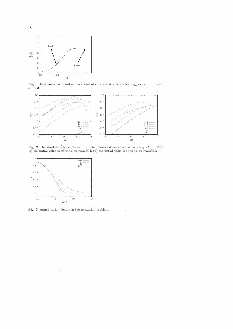
In a stiff case, characterized by λ << 1, the solution of the evolution equation
consists of two phases: a fast phase where there is a rapid approach to a slow manifold
followed by a slow phase where the solution evolves along the slow manifold (Cox and
Matthews, 2002), see Fig. 1. In the slow manifold the internal stress is given by (Cox
and Matthews, 2002; Boyd, 2001)
σ∗(t) = Eλdε
dt− Eλ2 d
2ε
dt2+ Eλ3 d
3ε
dt3− + . . . (2)
for the Maxwell model.
Since the ordinary differential equation (ODE) (1) involves a time derivative of the
strain, it is advantageous for numerical purposes to transform the ODE to form
y′(t) = F (t, y(t)) = −1
λy(t) +
E
λε(t) (3)
by using a change of variables σ∗(t) = Eε(t) − y(t). The numerical scheme of the
transformed ODE can be transformed back to the original variable σ∗ by using again
the change of variables. The naming convention of the integrators is based on the
integrators of the transformed ODE (3).

4
2.1 Runge-Kutta methods
An s-stage implicit Runge-Kutta (RK) method for the transformed ODE (3) is given
by
yn+1 = yn +∆ts∑
i=1
biki, (4)
ki = F
tn + ci∆t, yn +∆ts∑
j=1
aijkj
i = 1, . . . , s, (5)
where aij , bi, ci are the coefficients of the method and ∆t = tn+1 − tn is the step-size.
The backward Euler method for the Maxwell model is given by
σ∗n+1 =1
1 +∆t/λσ∗n +
E∆ε
1 +∆t/λ(bE), (6)
where ∆ε = ε(tn+1) − ε(tn) is the strain increment1. The trapezoidal or two-stage
Lobatto IIIA method is given by
σ∗n+1 =1 − 1
2∆t/λ
1 + 12∆t/λ
σ∗n +E∆ε
1 + 12∆t/λ
(Tr), (7)
and the two-stage Lobatto IIIC method by
σ∗n+1 =σ∗n + (1 + 1
2∆t/λ)E∆ε
1 +∆t/λ+ 12 (∆t/λ)2
(L3C). (8)
According to Kouhia et al. (2005), the integrator of an inelastic material model
should be at least L-stable, and for the ODE (1) without the source term, the am-
plification factor should be positive and monotonous. Both the backward Euler and
Lobatto IIIC methods fulfil these criteria. However, the trapezoidal method is only
A-stable, i.e. the amplification factor of the trapezoidal method doesnt’t approach zero
as ∆t/λ → ∞. Nevertheless, as it is well known, the trapezoidal method is a good
choice if the time step is sufficiently small. For more details on Lobatto methods and
stability properties of RK methods we refer to Hair and Wanner (1991).
The considered RK methods are closely related to Galerkin methods in time. The
backward Euler and trapezoidal methods can also be derived by applying the Galerkin
methods directly to the ODE (1). The backward Euler is equivalent to the discontinuous
Galerkin method of degree zero and the trapezoidal method is equivalent to the con-
tinuous Petrov-Galerkin method of degree one2. The performance of several Galerkin
methods for creep type inelastic models has been evaluated in Reference Kouhia et al.
(2005).
We would like to emphasize that the RK methods can be extended to handle
thermal (thermorheologically simple models) and nonlinear (Schapery type models)
effects as long as the kernel function is represented via the Prony series, i.e. constitutive
equation can be expressed in differential form.
1 (•)(tm) denotes the exact solution at time tm whereas (•)m denotes the numerical solutionat time tm, m ∈ {n, n+ 1}.
2 For the Galerkin methods we use definitions given in Reference Kouhia et al. (2005).

5
2.2 Semi-analytical methods
For viscoelastic materials the most popular time integrators are based on idealized
loading programs in which simplified variation of strain is assumed within a time step.
In what follows we adopt the name semi-analytical (SA) integrators for these types
of methods. To be more specific, we define SA integrators as methods in which the
evolution equation is integrated exactly by approximating strain by a continuous or
discontinuous polynomial within a time step.
The exact solution for the transformed ODE is given by
y(tn+1) = e−∆t/λy(tn) +E
λ
∫ tn+1
tn
e−(tn+1−τ)/λε(τ )dτ. (9)
The simplest approximation to evaluate the integral analytically is to assume that
the strain is constant throughout the time interval. Approximating ε(τ ) in a backward
manner, i.e. ε(τ ) = εn+1, and transforming the resulting scheme to the original variable
yields
σ∗n+1 = e−∆t/λσ∗n + e−∆t/λE∆ε (SA1). (10)
The SA1 method was first introduced by Zienkiewicz et al. (1968) for a Kelvin system.
A better approximation to the integral is to assume piecewise constant variation of
strain which gives
σ∗n+1 = e−∆t/λσ∗n + e−∆t/(2λ)E∆ε (SA2). (11)
This scheme is often derived by integrating the evolution equation exactly (see Eq.
(18)) and then using the midpoint rule to the integral and the center difference scheme
to the time derivative of strain, see e.g. Simo and Hughes (1998) and also Feng (1992).
Rather than approximating strain in a constant manner, we may approximate the
strain rate to be constant. Linear variation of strain gives
σ∗n+1 = e−∆t/λσ∗n +1 − e−∆t/λ
∆t/λE∆ε (SA3). (12)
The SA3 method is commonly attributed to Taylor et al. (1970). For small ∆t/λ the
second term of the right-hand side of Eq. (12) suffers from cancellation error. Thus, to
avoid rounding errors a series expansion should be used when ∆t/λ is small
1 − e−∆t/λ
∆t/λ= 1 −
1
2
(∆t
λ
)+
1
6
(∆t
λ
)2
− + . . . . (13)
The considered SA schemes have also been extended to nonlinear viscoelastic mod-
els. The constant and piecewise constant schemes have been generalized to the nonlinear
creep-based Schapery’s model by Beijer and Spoormaker (2002). For Schapery’s model
a time integration method which reduces in a linear case to the SA3 method was de-
rived by Henriksen (1984) and has been used by many other researchers (Czyz and
Szyszkowski, 1999; Lai and Bakker, 1996; Kennedy, 1998; Haj-Ali and Muliana, 2004).
Rather interestingly, we see that the only difference between the SA3 method and
the trapezoidal and Lobatto IIIC methods is the order of approximation of the expo-
nential function. We may rewrite Eqs. (7), (8) and (12) as
σ∗n+1 = Q(−∆t/λ)σ∗n +1 −Q(−∆t/λ)
∆t/λE∆ε, (14)
6
where Q(z) is the exponential function for the SA3 method, the diagonal (1,1)-Pade
approximation for the trapezoidal method and the subdiagonal (0,2)-Pade approxima-
tion for the Lobatto IIIC method. Similarly, we see that the SA1 method reduces to the
backward Euler method when the (0,1)-Pade approximation is used to the exponential.
Another interesting observation can be made when λ is small. In that case the first
term in the series (2) is recovered for the SA3 method as well as for the backward
Euler and Lobatto IIIC methods. Note the interesting behavior of the backward Euler
method. For large λ the backward Euler method approaches the SA1 method while for
small λ the backward Euler method approaches the SA3 method.
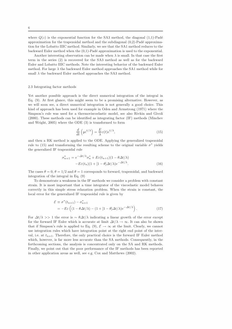
2.3 Integrating factor methods
Yet another possible approach is the direct numerical integration of the integral in
Eq. (9). At first glance, this might seem to be a promising alternative. However, as
we will soon see, a direct numerical integration is not generally a good choice. This
kind of approach has been used for example in Oden and Armstrong (1971) where the
Simpson’s rule was used for a thermoviscoelastic model, see also Rivkin and Givoli
(2000). These methods can be identified as integrating factor (IF) methods (Minchev
and Wright, 2005) where the ODE (3) is transformed to form
d
dt
(yet/λ
)=E
λε(t)et/λ, (15)
and then a RK method is applied to the ODE. Applying the generalized trapezoidal
rule to (15) and transforming the resulting scheme to the original variable σ∗ yields
the generalized IF trapezoidal rule
σ∗n+1 = e−∆t/λσ∗n + Eε(tn+1)(1 − θ∆t/λ)
−Eε(tn)(1 + [1 − θ]∆t/λ)e−∆t/λ. (16)
The cases θ = 0, θ = 1/2 and θ = 1 corresponds to forward, trapezoidal, and backward
integration of the integral in Eq. (9)
To demonstrate a weakness in the IF methods we consider a problem with constant
strain. It is most important that a time integrator of the viscoelastic model behaves
correctly in this simple stress relaxation problem. When the strain is constant, the
local error for the generalized IF trapezoidal rule is given by
E ≡ σ∗(tn+1) − σ∗n+1
= −Eε((1 − θ∆t/λ) − (1 + [1 − θ]∆t/λ)e−∆t/λ
). (17)
For ∆t/λ >> 1 the error is ∼ θ∆t/λ indicating a linear growth of the error except
for the forward IF Euler which is accurate at limit ∆t/λ → ∞. It can also be shown
that if Simpson’s rule is applied to Eq. (9), E → ∞ at the limit. Clearly, we cannot
use integration rules which have integration point at the right end point of the inter-
val, i.e. at tn+1. Therefore, the only practical choice is the forward IF Euler method
which, however, is far more less accurate than the SA methods. Consequently, in the
forthcoming sections, the analysis is concentrated only on the SA and RK methods.
Finally, we point out that the poor performance of the IF methods has been reported
in other application areas as well, see e.g. Cox and Matthews (2002).

7
3 Local error analysis
For the local error analysis we follow the approach taken in Reference Kværnø (2004).
In addition, it is assumed that the strain is independent of relaxation time λ.
The exact solution for the evolution equation of a Maxwell element is given by
σ∗(tn+1) = e−∆t/λσ∗(tn) + Ee−∆t/λ∫ ∆t
0eτ/λ d
dτε(tn + τ )dτ. (18)
Without loss of generality, we may assume hereafter that E = 1 or equivalently we
may consider the dimensionless form of the evolution equation. By expanding ε(tn +τ )
into a Taylor series gives
σ∗(tn+1) = e−∆t/λσ∗(tn) +∞∑
k=1
ε(k)(tn)1
(k − 1)!
× e−∆t/λ∫ ∆t
0eτ/λτk−1dτ. (19)
After integrating each term separately, we get
σ∗(tn+1) = ϕ0(∆t/λ)σ∗(tn) +
∞∑
k=1
ϕk(∆t/λ)ε(k)(tn)∆tk, (20)
where
ϕk(z) =1
(−z)k
e−z −k−1∑
j=0
(−z)j
j!
k = 1, 2, . . . , (21)
and ϕ0(z) = exp(−z) by definition.
The RK and SA methods can be written in a uniform form as
σ∗n+1 = ψ0(∆t/λ)σ∗n + ψ1(∆t/λ)E∆ε. (22)
In the following, it is assumed that the exact solution is known at time tn, i.e. σ∗n =
σ∗(tn). Functions ψ0(z) and ψ1(z) for the methods are given in Table 1. By expanding
ε(tn+1) we arrive at the following formula
σ∗n+1 = ψ0(∆t/λ)σ∗(tn) +∞∑
k=1
ψk(∆t/λ)ε(k)(tn)∆tk, (23)
where ψk(z) =ψ1(z)
k!.
By subtracting Eq. (23) from Eq. (20) we obtain the local truncation error
σ∗(tn+1) − σ∗n+1 = E0(∆t/λ)σ∗(tn)
+∞∑
k=1
Ek(∆t/λ)ε(k)(tn)∆tk, (24)
where the error function is Ek(z) = ϕk(z)−ψk(z). When σ∗(tn) is on the slow manifold
(see Eq. (2)), then the truncation error is
σ∗(tn+1) − σ∗n+1 =∞∑
k=1
Ek(∆t/λ)ε(k)(tn)∆tk, (25)
where Ek(z) = Ek(z) − E0(z)/(−z)k.

8
3.1 Nonstiff case
In the nonstiff case, ∆t/λ << 1, we express the error functions in terms of a Taylor
series expansion. The dominant terms of the error functions are given in Tables 2 and
3. Then, by inserting the dominant terms into the truncation error equation we obtain
the local errors. For the first-order accurate methods the errors are given by
EbE ≈1
2·
1
λ2
[−σ∗(tn) + λε′(tn)
]∆t2, (26)
ESA1 ≈1
2·1
λε′(tn)∆t2, (27)
and for the higher-order methods
ETr ≈1
12·
1
λ3
[σ∗(tn) − λε′(tn) + λ2ε′′(tn)
]∆t3, (28)
EL3C ≈1
12·
1
λ3
[−2σ∗(tn) + 2λε′(tn) + λ2ε′′(tn)
]∆t3, (29)
ESA2 ≈1
12·
1
λ2
[1
2ε′(tn) + λε′′(tn)
]∆t3, (30)
ESA3 ≈1
12·1
λε′′(tn)∆t3. (31)
The results are as expected. When λ << 1 and σ∗(tn) is on the slow manifold, the
errors for the RK methods are given by
EbE ≈
[1
2ε′′(tn) + O (λ)
]∆t2, (32)
ETr ≈
[1
12ε′′′(tn) + O (λ)
]∆t3, (33)
EL3C ≈
[1
4
1
λε′′(tn) −
1
6ε′′′(tn) + O (λ)
]∆t3. (34)
In this case the error of the backward Euler and trapezoidal methods is almost inde-
pendent of λ whereas for the Lobatto IIIC method the error behaves similarly as for
the SA3 method.
3.2 Stiff case
In the stiff case, ∆t/λ >> 1, we ignore the exponential terms and expand the error
functions as a function of (∆t/λ)−1. The dominant terms are given in Tables 4 and 5.
The local errors are now given by
EL3C ≈ 2λ2[−σ∗(tn) + λε′(tn)
]1
∆t2, (35)
EbE ≈ λ
[−σ∗(tn) + λε′(tn)
]1
∆t, (36)
ETr ≈ σ∗(tn) − λε′(tn) + λ2ε′′(tn), (37)
ESA1 ≈ λε′(tn), (38)
ESA2 ≈ λε′(tn), (39)
ESA3 ≈1
2λε′′(tn)∆t. (40)

9
The local errors behave rather differently as a function of the time step. For the back-
ward Euler and for Lobatto IIIC methods, the error decreases as the step size increases.
For the trapezoidal, SA1 and SA2 methods the leading error term is independent of
the time step. In addition, the error is approximately the same for the SA1 and SA2
methods. Once again, the best choice seems to be the SA3 method. However, in the
slow manifold case the error of the trapezoidal method has a quadratic dependency on
the time step
EbE ≈ EL3C ≈1
2λε′′(tn)∆t, (41)
ETr ≈1
6λε′′′(tn)∆t2, (42)
Furthermore, the error is now the same for the SA3, backward Euler and Lobatto IIIC
methods.
3.3 A numerical example
We consider a differential equation
dσ∗(t)
dt= −
1
λσ∗(t) +
d
dt(− cos t), σ∗(t0) = σ∗0 , (43)
with initial conditions
σ∗0 = 1 (off the slow manifold), (44)
σ∗0 =λ
1 + λ2(sin t0 − λ cos t0) (on the slow manifold). (45)
where t0 = π/4. The exact solution is given by
σ∗(t) =
(σ∗0 −
λ
1 + λ2(sin t0 − λ cos t0)
)e−(t−t0)/λ
+λ
1 + λ2(sin t− λ cos t). (46)
The errors after one time step are shown in Fig. 2. The numerical results are in
accordance with the theoretical predictions. We see that in the stiff case the error is
almost the same for the SA1 and SA2 methods and for the backward Euler and Lobatto
IIIC methods the error decreases as the time step increases. In the slow manifold case
we see that the error is approximately the same for the backward Euler, Lobatto IIIC
and SA3 methods when ∆t/λ >> 1. In addition, the trapezoidal method produces the
lowest error.
4 Uniaxial Maxwell solid
4.1 Constitutive model
We consider a linearly viscoelastic constitutive equation of the form
σ(t) =
∫ t
−∞
E(t− τ )ε(τ )dτ, (47)
10
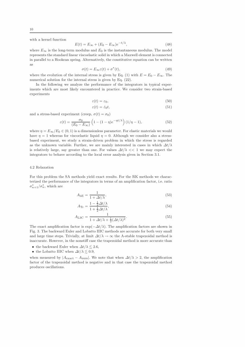
with a kernel function
E(t) = E∞ + (E0 − E∞)e−t/λ, (48)
where E∞ is the long-term modulus and E0 is the instantaneous modulus. The model
represents the standard linear viscoelastic solid in which a Maxwell element is connected
in parallel to a Hookean spring. Alternatively, the constitutive equation can be written
as
σ(t) = E∞ε(t) + σ∗(t), (49)
where the evolution of the internal stress is given by Eq. (1) with E = E0 − E∞. The
numerical solution for the internal stress is given by Eq. (22).
In the following we analyze the performance of the integrators in typical exper-
iments which are most likely encountered in practice. We consider two strain-based
experiments
ε(t) = ε0, (50)
ε(t) = ε0t, (51)
and a stress-based experiment (creep, σ(t) = σ0)
ε(t) =σ0
(E0 −E∞)
(1 − (1 − η)e−ηt/λ
)(1/η − 1), (52)
where η = E∞/E0 ∈ (0, 1) is a dimensionless parameter. For elastic materials we would
have η = 1 whereas for viscoelastic liquid η = 0. Although we consider also a stress-
based experiment, we study a strain-driven problem in which the stress is regarded
as the unknown variable. Further, we are mainly interested in cases in which ∆t/λ
is relatively large, say greater than one. For values ∆t/λ << 1 we may expect the
integrators to behave according to the local error analysis given in Section 3.1.
4.2 Relaxation
For this problem the SA methods yield exact results. For the RK methods we charac-
terized the performance of the integrators in terms of an amplification factor, i.e. ratio
σ∗n+1/σ∗
n, which are
AbE =1
1 +∆t/λ, (53)
ATr =1 − 1
2∆t/λ
1 + 12∆t/λ
, (54)
AL3C =1
1 +∆t/λ+ 12 (∆t/λ)2
. (55)
The exact amplification factor is exp(−∆t/λ). The amplification factors are shown in
Fig. 3. The backward Euler and Lobatto IIIC methods are accurate for both very small
and large time steps. Trivially, at limit ∆t/λ→ ∞ the A-stable trapezoidal method is
inaccurate. However, in the nonstiff case the trapezoidal method is more accurate than
• the backward Euler when ∆t/λ . 2.6,
• the Lobatto IIIC when ∆t/λ . 0.9,
when measured by |Aexact − Anum|. We note that when ∆t/λ > 2, the amplification
factor of the trapezoidal method is negative and in that case the trapezoidal method
produces oscillations.

11
4.3 Constant strain rate problem
To begin with, we illustrate in Fig. 4 the typical performance of the integrators in a
constant strain rate case. The numerical solution of the backward Euler and Lobatto
IIIC methods follows the true solution smoothly whereas for the SA1 and SA2 methods
the numerical solution diverges from the true solution after the transient phase. The
most notable difference is observed between the backward Euler and SA2 methods.
After the transient phase, asymptotically only first-order accurate Euler scheme is
more accurate than the second-order accurate SA2 method. The SA3 method gives
exact result for the constant strain rate problem.
To verify the observations let us first analyze a case where the solution approaches
the steady-state solution σ∗ = (E0 −E∞)λε0. When the strain increment is constant,
the recursive relation (22) yields a geometric series and therefore the numerical solution
can be expressed in a closed form. When time tends to infinity, i.e. n→ ∞, the solution
is given by
σ∗ = (E0 −E∞)λε0 ·∆t
λ
ψ1(∆t/λ)
1 − ψ0(∆t/λ)
≡ (E0 −E∞)λε0 · f(∆t/λ). (56)
The RK methods produce a correct limit value irrespective of the size of the time
step. For the SA1 and SA2 methods f(∆t/λ) decreases rapidly as ∆t/λ increases. In
the stability limit of the forward Euler method we find that f(2) ≈ 0.31 for the SA1
method and f(2) ≈ 0.85 for the SA2 method.
In the transient phase we may expect the SA methods to perform reasonably well.
This is illustrated in Fig. 5 where the relative errors after the first time step are
shown. For small time steps the SA2 method is the most accurate. However, even the
backward Euler method is more accurate than the SA2 method when the time step is
large enough. For large time steps the best choice is the Lobatto IIIC method.
Finally, we point out that we may expect the integrators to perform similarly also
in a constant stress rate case since in that case, too, the strain rate tends to a constant
value after a transient phase.
4.4 Creep
In the case of creep, the exact amplification factor is exp(−η∆t/λ). The local error is
given by
σ∗(tn+1) − σ∗n+1 = e−η∆t/λσ∗(tn) − σ∗n+1
= e−η∆t/λσ∗(tn) − ψ0(∆t/λ)σ∗(tn)
−ψ1(∆t/λ)(E0 − E∞)∆ε
= e−η∆t/λσ∗(tn)
−
(ψ0(∆t/λ) + ψ1(∆t/λ)
× (1 − 1/η)(e−η∆t/λ − 1)
)σ∗(tn)
≡ (Aexact −Anum)σ∗(tn), (57)
12
where Anum can be viewed as the ”local” amplification factor.
In the limit ∆t/λ → ∞ all of the methods are accurate except the trapezoidal
method. However, the amplification factors behave rather differently as ∆t/λ increases.
When η is small, the amplification factors of the SA1 and SA2 methods approach the
limit value rapidly, whereas for the backward Euler, Lobatto IIIC and SA3 methods,
a slower but smoother behavior is observed, see Fig. 6. From Fig. 6 it can also be seen
that the trapezoidal method performs considerably well even for large ∆t/λ. Clearly, for
stress-based experiments, the retardation time τ = λ/η > λ, which is a time constant
of the creep compliance, characterizes the stiffness of the problem. Consequently, the
stability of the integrator of the viscoelastic model should be tested for a relaxation
type problem rather than for a creep type problem.
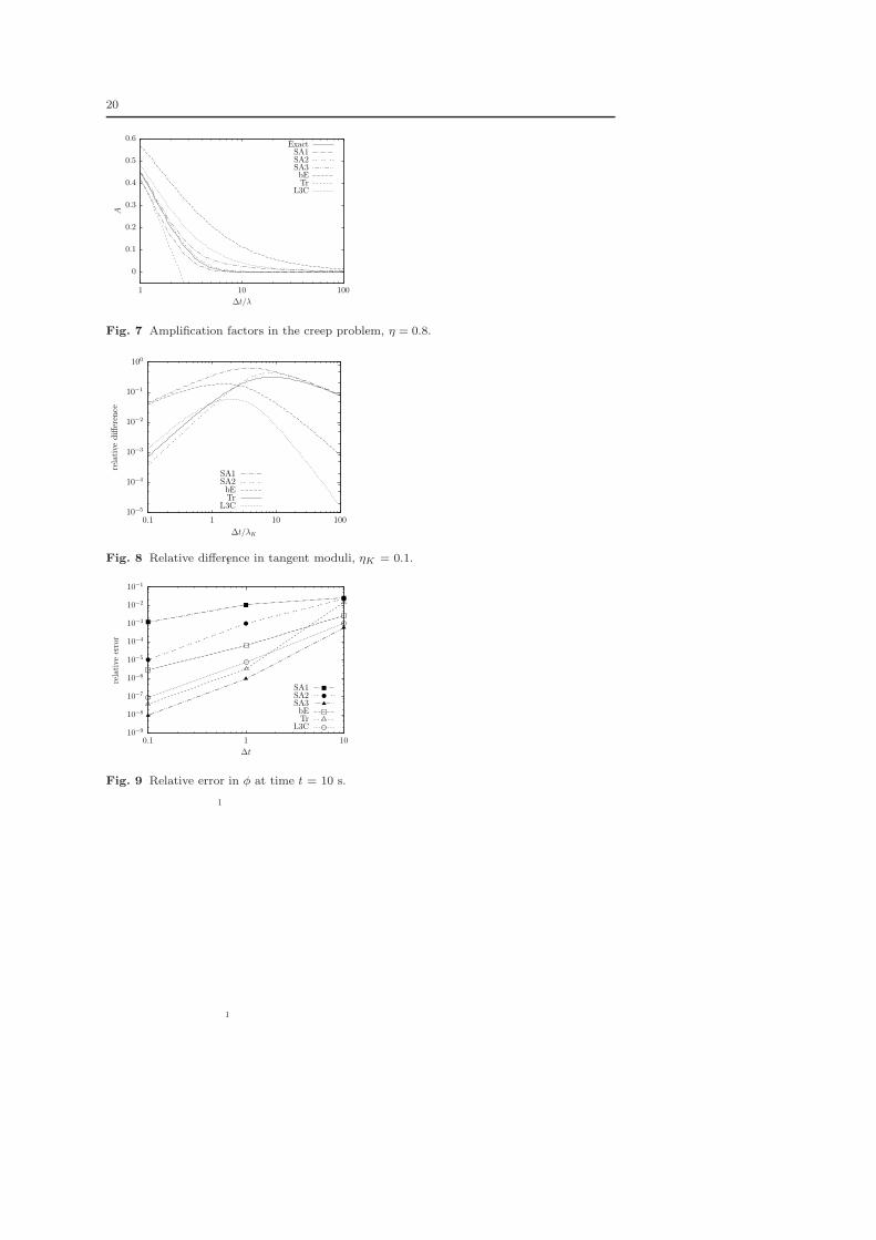
For a nearly elastic material, the SA methods perform considerably better than the
RK methods. This is shown in Fig. 7.
5 Multiaxial material model
5.1 Material model
We consider an isotropic constitutive model where the total stress σ = [σ11 σ22 σ33 σ12 σ13 σ23]T
and strain ε = [ε11 ε22 ε33 ε12 ε13 ε23]T are decomposed into deviatoric and volumetric
parts
σ(t) = s(t) + mp(t), (58)
ε(t) = e(t) +1
3mφ(t), m = [1 1 1 0 0 0]T, (59)
where s is the deviatoric stress, p = 13mT
σ is the mean stress, e is the deviatoric strain
and φ = mTε is the volume change. The deviatoric stress is given by
s(t) = 2
∫ t
0G(t− τ )e(τ )dτ, (60)
where G(t) is the shear modulus and the mean stress is given by
p(t) =
∫ t
0K(t− τ )φ(τ )dτ, (61)
where K(t) is the bulk modulus. We assume that the bulk and shear moduli are given
by
K(t) = K∞ + (K0 −K∞)e−t/λK ,
G(t) = G∞ + (G0 −G∞)e−t/λG .(62)
Corresponding compliances for bulk and shear are
B(t) = B0 + (B∞ −B0)(1 − e−t/τB),
J(t) = J0 + (J∞ − J0)(1 − e−t/τJ ),(63)
where
B0 =1
K0, B∞ =
1
K∞
, τB = λKK0
K∞
, (64)
J0 =1
G0, J∞ =
1
G∞
, τJ = λGG0
G∞
. (65)

13
5.2 Stress integration procedure
The numerical solution for stress is given by
σn+1 = sn+1 + mpn+1
= 2G∞e(tn+1) + s∗
n+1 +K∞mφ(tn+1) + mp∗n+1, (66)
in which
s∗
n+1 = ψ0(∆t/λG)s∗n + 2ψ1(∆t/λG)(G0 −G∞)∆e,
p∗n+1 = ψ0(∆t/λK)p∗n + ψ1(∆t/λK)(K0 −K∞)∆φ,(67)
where the functions ψ0(z) and ψ1(z) for the SA and RK methods are given in Table 1.
The consistent tangent operator, which will be needed in the forthcoming analysis
and which is also very important when solving nonlinear finite element (FE) equations,
is given by
CT =∂σn+1
∂ε(tn+1)= 2
[G∞ + ψ1(∆t/λG)(G0 −G∞)
] [I −
1
3mm
T]
+
[K∞ + ψ1(∆t/λK)(K0 −K∞)
]mm
T. (68)
where I is the identity matrix. To get a rough idea of the relative difference of the
various tangent moduli we compare the volumetric part of the moduli. The volumetric
part can be given in form
[1 + ψ1(∆t/λK)(1/ηK − 1)
]C
∗, (69)
where ηK = K∞/K0 ∈ (0, 1) is a dimensionless parameter and C∗ = K∞mmT is a
common factor. The relative difference can be now computed as a function of ηK and
∆t/λK . The exact tangent operator is problem-dependent. Thus, the SA3 method,
which is perhaps the most commonly used method in practical applications (Abaqus,
2004; Taylor, 2008) and is very accurate according to the local error analysis, was
chosen as the reference method. The relative difference is shown in Fig. 8 using the
value ηK = 0.1 for the dimensionless parameter. It is seen that for small time steps
the SA2 method is closest to the SA3 method. For the backward Euler and Lobatto
IIIC methods the difference significantly decreases once the maximum difference is
attained. Consequently, for large time steps the Lobatto IIIC method is closest to the
SA3 method.
5.3 Uniaxial tension
We consider a problem where the isotropic material is subjected to uniaxial stress
σ11(t) = σ0t where σ0 = 0.5 kPa. In this case we try to find the solution for the
volume change and for the deviatoric strain components. The exact solutions for the
volume change and for the deviatoric strain component in 1-direction are given by
φ(t) =1
3(B ∗ σ11)(t), e11(t) =
1
3(J ∗ σ11)(t), (70)
14
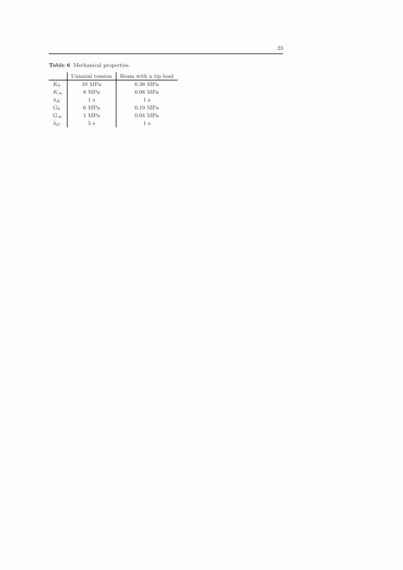
where ∗ is the convolution operator. The material parameters are given in Table 6.
The solution for the strain components is found by solving a residual equation
σ(tn+1) − σn+1(εn+1) = 0, (71)
using the Newton-Raphson method
εk+1n+1 = ε
kn+1 + C
−1T
(σ(tn+1) − σn+1(ε
kn+1)
). (72)
where k is the iteration number, σ(tn+1) is the exact stress vector and σn+1 is the
computed stress vector. Since the residual equation is linear, the Newton-Raphson
method converges in one iteration. Once convergence is achieved, the volume change
and deviatoric strain components are computed and the internal stress variables are
updated.
The relative error at time t = 10 s is shown as a function of the time step in Figs.
9 and 10. For the deviatoric part the problem is nonstiff and thus for the deviatoric
strain component the first-order accurate SA1 and backward Euler methods produce
largest errors. For the volume part the problem is stiffer, the time constants, λK and
τB , are order of a second. Furthermore, at time t = 10 s the transient phase, due to the
exponential function, has completely damped out. In this case the performance of the
SA1 and SA2 methods decreases. Even for a time step of size 0.1 s the backward Euler
is more accurate than the SA2 method. This is consistent with the observation made
in Section 4.3. Further, we see that for the trapezoidal method the error drastically
increases as the time step is increased from 1 s to 10 s. The Lobatto IIIC and SA3
methods behave similarly in both cases, the only difference is that the relative error is
slightly higher for the Lobatto IIIC method.
5.4 FEM-example: beam with a tip load
A beam with a tip load F (t) = F0H(t) is analyzed, see Fig. 11. This problem has
been previously considered in References Poon and Ahmad (1998); Zocher and Groves
(1997). The length L of the beam is 20 m and the beam has a rectangular cross-section
of size 1 m × 1 m. The solution for the tip displacement, according to Euler-Bernoulli
beam theory, is given by
w(t) =F0L
3
27I
[3J(t) +B(t)
], (73)
where I is the area moment of inertia of the beam. The physical properties of the beam
are given in Table 6.
The isotropic model was implemented in the commercial FE-code ABAQUS using
the user subroutine UMAT. The step function H(t) was modeled by a ramp history
wherein the force was increased to a constant value in a single time increment of size
10−4 s. The size of the load F0 was 1 N. A mesh consisting of 10 × 10 × 200 elements
was used in the analysis. The time step was fixed at 5 s.
The simulation results are shown in Fig. 12. The results are in accordance with the
uniaxial creep case. Compared to the backward Euler, Lobatto IIIC and SA3 methods,
the numerical solution of the SA1 and SA2 methods reaches the steady-state solution
rapidly. Again, the trapezoidal method performs extremely well although the time step
is relatively large compared to the relaxation times.

15
6 Concluding remarks
In this paper, the performance of various time integrators of the integral model of linear
viscoelasticity was studied. Both analytical and numerical analyses were presented.
The main results can be summarized as follows:
• The difference between the SA3, L3C and Tr methods, and between the SA1 and
bE methods is in the order of approximation of the exponential function.
• The bE and L3C methods are accurate for both a very small and a very large time
step. For nonstiff problems, say ∆t/λ < 2, the Tr method can be considered to be
the best choice among the RK methods.
• According to the local error analysis, the accuracy of the RK methods depends
strongly on whether the initial values are on the slow manifold or not.
• For stiff problems we may expect the SA3, L3C and bE methods to behave in
a similar fashion. A similar conclusion can be drawn between the SA1 and SA2
methods.
• The SA3, L3C and bE methods seem to behave more smoothly than the SA1 and
SA2 methods. This should be noted if a notable change is made in the size of the
time step.
• The stability analysis should be performed for a relaxation type problem rather
than for a creep type problem.
• As regards the asymptotically first-order accurate methods, the bE method is a
better choice than the SA1 method.
• Considering the overall performance of the integrators, the SA3 method is a superior
choice. However, the L3C method behaves very similarly to the SA3 method.
Finally, we would like to point out that the analysis was focused on the relaxation-
based material model. That is, we assumed that the relaxation modulus is the known
material function. For nonlinear models, such as Schapery’s model, the creep-based
material model is often used. The results derived herein cannot be directly extended
to creep-based models.
Acknowledgements The authors wish to acknowledge the assistance of Matti Malinen fromKuava Ltd.
References
Abaqus: Abaqus/Standard, Theory Manual. Version 6.5. Hibbitt, Karlsson and Soren-
son, Inc., Pawtucket (2004)
Argyris J., Doltsinis I.St., da Silva V.D.: Constitutive modelling and computation of
non-linear viscoelastic solids. Part I: Rheological models and numerical integration
techniques. Comput. Meth. Appl. Mech. Eng. 88, 135-163 (1991)
Beijer J.G.J., Spoormaker J.L.: Solution strategies for FEM analysis with nonlinear
viscoelastic polymers. Comput. Struct. 80, 1213-1229 (2002)
Beylkin G., Keiser J., Vozovoi L.: A new class of time discretization schemes for the
solution of nonlinear PDEs. J. Comput. Phys. 147, 362-387 (2002)
Boyd J.P.: Chebyshev and Fourier spectral methods. Dover, New York (2001).
Buttner J., Simeon B. Runge-Kutta methods in elastoplasticity. Appl. Numer. Math.
41, 443-458 (2002)

16
Cox S.M., Matthews P.C.: Exponential time differencing for stiff systems. J. Comput.
Phys. 176, 430–455 (2002)
Czyz J.A., Szyszkowski W.: An efficient method for non-linear viscoelastic structural
analysis. Comput. Struct. 37, 637-646 (1990)
Dooling, P.J, Buckley C.P., Hinduja S.: An intermediate model method for obtaining
a discrete relaxation spectrum for creep data. Rheol. Acta 36, 472-482, (1997)
Feng, W.W.: A recurrence formula for viscoelastic constitutive equations. Int. J. Non-
Linear Mech. 27, 675-678, (1992)
Goh S.M., Charalambides M.N., Williams J.G.: Determination of the constitutive con-
stants of non-linear viscoelastic materials. Mech. Time-Depend. Mater. 8, 255-268
(2004)
Gramoll K.C., Dillard D.A., Brinson H.F.: A stable numerical solution method for
in-plane loading of non-linear viscoelastic laminated orthotropic materials. Compos.
Struct. 13, 251-274 (1989)
Hairer E., Wanner G.: Solving ordinary differential equations II, stiff and differential-
algebraic problems. Springer, Berlin (1991)
Haj-Ali R.M., Muliana A.H.: Numerical finite element formulation of the Schapery
non-linear viscoelastic material model. Int. J. Numer. Meth. Eng. 59, 25-45 (2004)
Henriksen M.: Nonlinear viscoelastic stress analysis - a finite element approach. Com-
put. Struct. 18, 133-139 (1984)
Herrman L.R., Peterson F.E.: A numerical procedure for viscoelastic stress analysis.
In: Proceedings of the Seventh Meeting of ICRPG Mechanical Behavior Working
Group, Orlando (1968)
Holzapfel G.A.: On large strain viscoelasticity: continuum formulation and finite ele-
ment applications to elastomeric structures. Int. J. Numer. Meth. Eng. 39, 3903-3926
(1996)
Hsu S.Y., Jain S.K., Griffin O.H.: Verification of endochronic theory for nonpropor-
tional loading paths. J. Eng. Mech. 117, 110-131 (1991)
Kennedy T.C.: Nonlinear viscoelastic analysis of composite plates and shells. Compos.
Struct. 41, 265-272 (1998)
Kirchner E., Kollmann F.G.: Application of modern time integrators to Hart’s inelastic
model. Int. J. Plast. 15, 647-666 (1999)
Kirchner E., Simeon B.: A higher-order time integration method for viscoplasticity.
Comput. Meth. Appl. Mech. Eng. 175, 1-18 (1999)
Knauss W.G., Zhao J.: Improved relaxation time coverage in ramp-strain histories.
Mech. Time-Depend. Mater. 11, 199-216 (2007)
Kouhia R., Marjamaki P., Kivilahti J.: On the implicit integration of rate-dependent
inelastic constitutive models. Int. J. Numer. Meth. Eng. 62, 1832-1856 (2005)
Kværnø A.: Time integration methods for coupled equations. Department of Mathe-
matical Sciences, Norwegian University of Science and Technology, Preprint Numer-
ics No. 7 (2004)
Lai J., Bakker A.: 3-D schapery representation for non-linear viscoelasticity and finite
element implementation. Comput. Mech. 18, 182-191 (1996)
Minchev B.V., Wright W.M.: A review of exponential integrators for first order semi-
linear problems. Department of Mathematical Sciences, Norwegian University of Sci-
ence and Technology, Preprint Numerics No. 2 (2005)
Oden J.T., Armstrong W.H.: Analysis of nonlinear, dynamic coupled thermoviscoelas-
ticity problems by the finite element method. Comput. Struct. 1, 603-621 (1971)

17
Patlashenko I., Givoli D., Barbone P.: Time-stepping schemes for systems of Volterra
integro-differential equations. Comput. Meth. Appl. Mech. Eng. 190, 5691-5718
(2001)
Poon H., Ahmad M.F.: A material point time integration procedure for anisotropic,
thermo rheologically simple, viscoelastic solids. Comput. Mech. 21, 236-242 (1998)
Poon H., Ahmad M.F.: A finite element constitutive update scheme for anisotropic,
viscoelastic solids exhibiting non-linearity of the schapery type. Int. J. Numer. Meth.
Eng. 46, 2027-2041 (1999)
Rivkin L., Givoli D.: An efficient finite element scheme for viscoelasticity with moving
boundaries. Comput. Mech. 24, 503-512 (2000)
Schapery R.A.: On the characterization of nonlinear viscoelastic materials. Polymer.
Eng. Sci. 9, 295-310 (1969)
Schapery R.A.: Nonlinear viscoelastic and viscoplastic constitutive equations based on
thermodynamics. Mech. Time-Depend. Mater. 1, 209-240 (1997)
Schreyer H.L., Kulak R.F., Kramer J.M.: Accurate numerical solutions for elastic-
plastic models. J. Pres. Vessel Tech. 101, 226-234 (1979)
Simo J.C., Kennedy J.G., Govindjee S.: Non-smooth multisurface plasticity and vis-
coplasticity. Loading/unloading conditions and numerical algorithms. Int. J. Numer.
Meth. Eng. 26, 2161-2185 (1988)
Simo J.C., Hughes T.J.R.: Computational inelasticity. Springer, New York (1998)
Sorvari J., Malinen M.: On the direct estimation of creep and relaxation functions.
Mech. Time-Depend. Mater. 11, 143-157 (2007)
Taylor R.L., Pister K.S., Goudreau G.L.: Thermomechanical analysis of viscoelastic
solids. Int. J. Numer. Meth. Eng. 2, 45-59 (1970)
Taylor R.L.: FEAP - a finite element analysis program, version 8.2, theory manual.
Department of Civil and Environmental Engineering, University of California at
Berkeley (2008).
Touati D., Cederbaum G.: Stress relaxation of nonlinear thermoviscoelastic materials
predicted from known creep. Mech. Time-Depend. Mater. 1, 321-330 (1998)
Zienkiewicz O.C., Watson M., King I.P.: A numerical method of visco-elastic stress
analysis. Int. J. Mech. Sci. 10, 807-827 (1968)
Zienkiewicz O.C., Taylor R.L.: The finite element method. Butterworth-Heinemann,
Oxford (2000)
Zocher M.A., Groves S.E.: A three-dimensional finite element formulation for thermo-
viscoelastic orthotropic media. Int. J. Numer. Meth. Eng. 40, 2267-2288 (1997)
Østerby O.: Five ways of reducing the Crank-Nicolson oscillations. BIT Numer. Math.
43, 811-822 (2003)
18
0
0.2
0.4
0.6
0.8
1
1.2
1.4
0.01 0.1 1 10
σ∗(t)
Eλε
t [s]
FAST
SLOW
1
Fig. 1 Fast and slow manifolds in a case of constant strain-rate loading, i.e. ε = constant,λ = 0.2.
10−12
10−10
10−8
10−6
10−4
10−2
100
10−4 10−3 10−2 10−1 100
erro
r
∆t
SA1SA2SA3bETr
L3C
1
10−12
10−10
10−8
10−6
10−4
10−2
100
10−4 10−3 10−2 10−1 100
erro
r
∆t
SA1SA2SA3bETr
L3C
1
Fig. 2 The absolute value of the error for the internal stress after one time step (λ = 10−2).(a) the initial value is off the slow manifold, (b) the initial value is on the slow manifold.
0
0.2
0.4
0.6
0.8
1
0.1 1 10 100
A
∆t/λ
ExactbETr
L3C
1
Fig. 3 Amplification factors in the relaxation problem.

19
0
0.2
0.4
0.6
0.8
1
1.2
0 2 4 6 8 10
σ∗(t)
E0 − E∞
t [s]
ExactSA1SA2bETr
L3C
1
Fig. 4 Constant strain-rate loading (ε0 = 1 s−1, λ = 1 s).
10−5
10−4
10−3
10−2
10−1
100
0.1 1 10 100
rela
tive
erro
r
∆t/λ
SA1SA2bETr
L3C
1
Fig. 5 Relative error after first time step in the constant strain rate loading case.
0
0.2
0.4
0.6
0.8
1
1 10 100
A
∆t/λ
ExactSA1SA2SA3bETr
L3C
1
Fig. 6 Amplification factors in the creep problem, η = 0.1.
20
0
0.1
0.2
0.3
0.4
0.5
0.6
1 10 100
A
∆t/λ
ExactSA1SA2SA3bETr
L3C
1
Fig. 7 Amplification factors in the creep problem, η = 0.8.
10−5
10−4
10−3
10−2
10−1
100
0.1 1 10 100
rela
tive
diff
eren
ce
∆t/λK
SA1SA2bETr
L3C
1
Fig. 8 Relative difference in tangent moduli, ηK = 0.1.
10−9
10−8
10−7
10−6
10−5
10−4
10−3
10−2
10−1
0.1 1 10
rela
tive
erro
r
∆t
SA1SA2SA3bETr
L3C
1
Fig. 9 Relative error in φ at time t = 10 s.

21
10−6
10−5
10−4
10−3
10−2
10−1
100
101
0.1 1 10
rela
tive
erro
r
∆t
SA1SA2SA3bETr
L3C
1
Fig. 10 Relative error in e11 at time t = 10 s.
F (t)
L
1
Fig. 11 Beam with a tip load.
0.1
0.15
0.2
0.25
0.3
0 5 10 15 20 25 30
w[m
]
t [s]
ExactSA1SA2SA3bETr
L3C
1
Fig. 12 Tip displacement.
Table 1 Functions ψk(z) for the numerical methods.
ψ0 ψ1
SA1 e−z e−z
SA2 e−z e−z/2
SA3 e−z 1−e−z
z
bE 1
1+z1
1+z
Tr1−z/2
1+z/2
1
1+z/2
L3C 1
1+z+z2/2
1+z/2
1+z+z2/2

22
Table 2 Error functions Ek(z) for the methods when z << 1.
E0 E1 E2
SA1 0 1
2z + O(z2) 1
3z + O(z2)
SA2 0 1
24z2 + O(z3) 1
12z + O(z2)
SA3 0 0 1
12z + O(z2)
bE − 1
2z2 + O(z3) 1
2z + O(z2) 1
3z + O(z2)
Tr 1
12z3 + O(z4) − 1
12z2 + O(z3) 1
12z + O(z2)
L3C − 1
6z3 + O(z4) 1
6z2 + O(z3) 1
12z + O(z2)
Table 3 Error functions Ek(z) for the methods when z << 1.
E1 E2 E3
bE 0 1
2+ O(z) − 1
2z+ O(1)
Tr 0 0 1
12+ O(z)
L3C 0 1
4z + O(z2) − 1
6+ O(z)
Table 4 Error functions Ek(z) for the methods when z >> 1.
E0 E1 E2
SA1 0 1
z+ O( 1
z2 ) 1
z+ O( 1
z2 )
SA2 0 1
z+ O( 1
z2 ) 1
z+ O( 1
z2 )
SA3 0 0 1
2z+ O( 1
z2 )
bE − 1
z+ O( 1
z2 ) 1
z2 + O( 1
z3 ) 1
2z+ O( 1
z2 )
Tr 1 + O( 1
z) − 1
z+ O( 1
z2 ) 1
z2 + O( 1
z3 )
L3C − 2
z2 + O( 1
z3 ) 2
z3 + O( 1
z4 ) 1
2z+ O( 1
z2 )
Table 5 Error functions Ek(z) for the methods when z >> 1.
E1 E2 E3
bE 0 1
2z+ O( 1
z2 ) 1
3z+ O( 1
z2 )
Tr 0 0 1
6z+ O( 1
z2 )
L3C 0 1
2z+ O( 1
z2 ) 1
3z+ O( 1
z2 )
23
Table 6 Mechanical properties.
Uniaxial tension Beam with a tip load
K0 10 MPa 0.38 MPa
K∞ 8 MPa 0.08 MPa
λK 1 s 1 s
G0 6 MPa 0.19 MPa
G∞ 1 MPa 0.04 MPa
λG 5 s 1 s