Title stata.com

ivregress — Single-equation instrumental-variables regression

Syntax Menu Description OptionsRemarks and examples Stored results Methods and formulas ReferencesAlso see

Syntax

ivregress estimator depvar[

varlist1](varlist2 = varlistiv)

[if] [

in] [

weight][

, options]

estimator Description

2sls two-stage least squares (2SLS)liml limited-information maximum likelihood (LIML)gmm generalized method of moments (GMM)

options Description

Model

noconstant suppress constant termhascons has user-supplied constant

GMM1

wmatrix(wmtype) wmtype may be robust, cluster clustvar, hac kernel, or unadjustedcenter center moments in weight matrix computationigmm use iterative instead of two-step GMM estimatoreps(#)2 specify # for parameter convergence criterion; default is eps(1e-6)

weps(#)2 specify # for weight matrix convergence criterion; default isweps(1e-6)

optimization options2 control the optimization process; seldom used

SE/Robust

vce(vcetype) vcetype may be unadjusted, robust, cluster clustvar, bootstrap,jackknife, or hac kernel

Reporting

level(#) set confidence level; default is level(95)

first report first-stage regressionsmall make degrees-of-freedom adjustments and report small-sample

statisticsnoheader display only the coefficient tabledepname(depname) substitute dependent variable nameeform(string) report exponentiated coefficients and use string to label themdisplay options control column formats, row spacing, line width, display of omitted

variables and base and empty cells, and factor-variable labeling

1

2 ivregress — Single-equation instrumental-variables regression

perfect do not check for collinearity between endogenous regressors andexcluded instruments

coeflegend display legend instead of statistics

1These options may be specified only when gmm is specified.2These options may be specified only when igmm is specified.varlist1, varlist2, and varlistiv may contain factor variables; see [U] 11.4.3 Factor variables.depvar, varlist1, varlist2, and varlistiv may contain time-series operators; see [U] 11.4.4 Time-series varlists.bootstrap, by, jackknife, rolling, statsby, and svy are allowed; see [U] 11.1.10 Prefix commands.Weights are not allowed with the bootstrap prefix; see [R] bootstrap.aweights are not allowed with the jackknife prefix; see [R] jackknife.hascons, vce(), noheader, depname(), and weights are not allowed with the svy prefix; see [SVY] svy.aweights, fweights, iweights, and pweights are allowed; see [U] 11.1.6 weight.perfect and coeflegend do not appear in the dialog box.See [U] 20 Estimation and postestimation commands for more capabilities of estimation commands.

MenuStatistics > Endogenous covariates > Single-equation instrumental-variables regression

Descriptionivregress fits a linear regression of depvar on varlist1 and varlist2, using varlistiv (along with

varlist1) as instruments for varlist2. ivregress supports estimation via two-stage least squares (2SLS),limited-information maximum likelihood (LIML), and generalized method of moments (GMM).

In the language of instrumental variables, varlist1 and varlistiv are the exogenous variables, andvarlist2 are the endogenous variables.

Options

� � �Model �

noconstant; see [R] estimation options.

hascons indicates that a user-defined constant or its equivalent is specified among the independentvariables.

� � �GMM �

wmatrix(wmtype) specifies the type of weighting matrix to be used in conjunction with the GMMestimator.

Specifying wmatrix(robust) requests a weighting matrix that is optimal when the error term isheteroskedastic. wmatrix(robust) is the default.

Specifying wmatrix(cluster clustvar) requests a weighting matrix that accounts for arbitrarycorrelation among observations within clusters identified by clustvar.

Specifying wmatrix(hac kernel #) requests a heteroskedasticity- and autocorrelation-consistent(HAC) weighting matrix using the specified kernel (see below) with # lags. The bandwidth of akernel is equal to # + 1.

ivregress — Single-equation instrumental-variables regression 3

Specifying wmatrix(hac kernel opt) requests an HAC weighting matrix using the specified kernel,and the lag order is selected using Newey and West’s (1994) optimal lag-selection algorithm.

Specifying wmatrix(hac kernel) requests an HAC weighting matrix using the specified kernel andN − 2 lags, where N is the sample size.

There are three kernels available for HAC weighting matrices, and you may request each one byusing the name used by statisticians or the name perhaps more familiar to economists:

bartlett or nwest requests the Bartlett (Newey–West) kernel;

parzen or gallant requests the Parzen (Gallant 1987) kernel; and

quadraticspectral or andrews requests the quadratic spectral (Andrews 1991) kernel.

Specifying wmatrix(unadjusted) requests a weighting matrix that is suitable when the errors arehomoskedastic. The GMM estimator with this weighting matrix is equivalent to the 2SLS estimator.

center requests that the sample moments be centered (demeaned) when computing GMM weightmatrices. By default, centering is not done.

igmm requests that the iterative GMM estimator be used instead of the default two-step GMM estimator.Convergence is declared when the relative change in the parameter vector from one iteration tothe next is less than eps() or the relative change in the weight matrix is less than weps().

eps(#) specifies the convergence criterion for successive parameter estimates when the iterative GMMestimator is used. The default is eps(1e-6). Convergence is declared when the relative differencebetween successive parameter estimates is less than eps() and the relative difference betweensuccessive estimates of the weighting matrix is less than weps().

weps(#) specifies the convergence criterion for successive estimates of the weighting matrix whenthe iterative GMM estimator is used. The default is weps(1e-6). Convergence is declared whenthe relative difference between successive parameter estimates is less than eps() and the relativedifference between successive estimates of the weighting matrix is less than weps().

optimization options: iterate(#),[no]log. iterate() specifies the maximum number of iterations

to perform in conjunction with the iterative GMM estimator. The default is 16,000 or the numberset using set maxiter (see [R] maximize). log/nolog specifies whether to show the iterationlog. These options are seldom used.

� � �SE/Robust �

vce(vcetype) specifies the type of standard error reported, which includes types that are robust tosome kinds of misspecification (robust), that allow for intragroup correlation (cluster clustvar),and that use bootstrap or jackknife methods (bootstrap, jackknife); see [R] vce option.

vce(unadjusted), the default for 2sls and liml, specifies that an unadjusted (nonrobust) VCEmatrix be used. The default for gmm is based on the wmtype specified in the wmatrix() option;see wmatrix(wmtype) above. If wmatrix() is specified with gmm but vce() is not, then vcetypeis set equal to wmtype. To override this behavior and obtain an unadjusted (nonrobust) VCE matrix,specify vce(unadjusted).

ivregress also allows the following:

vce(hac kernel[

# | opt]) specifies that an HAC covariance matrix be used. The syntax used

with vce(hac kernel . . .) is identical to that used with wmatrix(hac kernel . . .); seewmatrix(wmtype) above.

� � �Reporting �

level(#); see [R] estimation options.

4 ivregress — Single-equation instrumental-variables regression

first requests that the first-stage regression results be displayed.

small requests that the degrees-of-freedom adjustmentN/(N−k) be made to the variance–covariancematrix of parameters and that small-sample F and t statistics be reported, where N is the samplesize and k is the number of parameters estimated. By default, no degrees-of-freedom adjustmentis made, and Wald and z statistics are reported. Even with this option, no degrees-of-freedomadjustment is made to the weighting matrix when the GMM estimator is used.

noheader suppresses the display of the summary statistics at the top of the output, displaying onlythe coefficient table.

depname(depname) is used only in programs and ado-files that use ivregress to fit models other thaninstrumental-variables regression. depname() may be specified only at estimation time. depnameis recorded as the identity of the dependent variable, even though the estimates are calculated usingdepvar. This method affects the labeling of the output—not the results calculated—but couldaffect later calculations made by predict, where the residual would be calculated as deviationsfrom depname rather than depvar. depname() is most typically used when depvar is a temporaryvariable (see [P] macro) used as a proxy for depname.

eform(string) is used only in programs and ado-files that use ivregress to fit models otherthan instrumental-variables regression. eform() specifies that the coefficient table be displayed in“exponentiated form”, as defined in [R] maximize, and that string be used to label the exponentiatedcoefficients in the table.

display options: noomitted, vsquish, noemptycells, baselevels, allbaselevels, nofvla-bel, fvwrap(#), fvwrapon(style), cformat(% fmt), pformat(% fmt), sformat(% fmt), andnolstretch; see [R] estimation options.

The following options are available with ivregress but are not shown in the dialog box:

perfect requests that ivregress not check for collinearity between the endogenous regressors andexcluded instruments, allowing one to specify “perfect” instruments. This option cannot be usedwith the LIML estimator. This option may be required when using ivregress to implement otherestimators.

coeflegend; see [R] estimation options.

Remarks and examples stata.com

ivregress performs instrumental-variables regression and weighted instrumental-variables regres-sion. For a general discussion of instrumental variables, see Baum (2006), Cameron and Trivedi (2005;2010, chap. 6) Davidson and MacKinnon (1993, 2004), Greene (2012, chap. 8), and Wooldridge(2010, 2013). See Hall (2005) for a lucid presentation of GMM estimation. Angrist and Pischke (2009,chap. 4) offer a casual yet thorough introduction to instrumental-variables estimators, including theiruse in estimating treatment effects. Some of the earliest work on simultaneous systems can befound in Cowles Commission monographs—Koopmans and Marschak (1950) and Koopmans andHood (1953)—with the first developments of 2SLS appearing in Theil (1953) and Basmann (1957).However, Stock and Watson (2011, 422–424) present an example of the method of instrumentalvariables that was first published in 1928 by Philip Wright.

The syntax for ivregress assumes that you want to fit one equation from a system of equationsor an equation for which you do not want to specify the functional form for the remaining equationsof the system. To fit a full system of equations, using either 2SLS equation-by-equation or three-stageleast squares, see [R] reg3. An advantage of ivregress is that you can fit one equation of amultiple-equation system without specifying the functional form of the remaining equations.

ivregress — Single-equation instrumental-variables regression 5

Formally, the model fit by ivregress is

yi = yiβ1 + x1iβ2 + ui (1)

yi = x1iΠ1 + x2iΠ2 + vi (2)

Here yi is the dependent variable for the ith observation, yi represents the endogenous regressors(varlist2 in the syntax diagram), x1i represents the included exogenous regressors (varlist1 in the syntaxdiagram), and x2i represents the excluded exogenous regressors (varlistiv in the syntax diagram).x1i and x2i are collectively called the instruments. ui and vi are zero-mean error terms, and thecorrelations between ui and the elements of vi are presumably nonzero.

The rest of the discussion is presented under the following headings:

2SLS and LIML estimatorsGMM estimator

2SLS and LIML estimators

The most common instrumental-variables estimator is 2SLS.

Example 1: 2SLS estimator

We have state data from the 1980 census on the median dollar value of owner-occupied housing(hsngval) and the median monthly gross rent (rent). We want to model rent as a function ofhsngval and the percentage of the population living in urban areas (pcturban):

renti = β0 + β1hsngvali + β2pcturbani + ui

where i indexes states and ui is an error term.

Because random shocks that affect rental rates in a state probably also affect housing values, wetreat hsngval as endogenous. We believe that the correlation between hsngval and u is not equalto zero. On the other hand, we have no reason to believe that the correlation between pcturban andu is nonzero, so we assume that pcturban is exogenous.

Because we are treating hsngval as an endogenous regressor, we must have one or more additionalvariables available that are correlated with hsngval but uncorrelated with u. Moreover, these excludedexogenous variables must not affect rent directly, because if they do then they should be includedin the regression equation we specified above. In our dataset, we have a variable for family income(faminc) and for region of the country (region) that we believe are correlated with hsngval butnot the error term. Together, pcturban, faminc, and factor variables 2.region, 3.region, and4.region constitute our set of instruments.

To fit the equation in Stata, we specify the dependent variable and the list of included exogenousvariables. In parentheses, we specify the endogenous regressors, an equal sign, and the excludedexogenous variables. Only the additional exogenous variables must be specified to the right of theequal sign; the exogenous variables that appear in the regression equation are automatically includedas instruments.

6 ivregress — Single-equation instrumental-variables regression

Here we fit our model with the 2SLS estimator:

. use http://www.stata-press.com/data/r13/hsng(1980 Census housing data)

. ivregress 2sls rent pcturban (hsngval = faminc i.region)

Instrumental variables (2SLS) regression Number of obs = 50Wald chi2(2) = 90.76Prob > chi2 = 0.0000R-squared = 0.5989Root MSE = 22.166

rent Coef. Std. Err. z P>|z| [95% Conf. Interval]

hsngval .0022398 .0003284 6.82 0.000 .0015961 .0028836pcturban .081516 .2987652 0.27 0.785 -.504053 .667085

_cons 120.7065 15.22839 7.93 0.000 90.85942 150.5536

Instrumented: hsngvalInstruments: pcturban faminc 2.region 3.region 4.region

As we would expect, states with higher housing values have higher rental rates. The proportionof a state’s population that is urban does not have a significant effect on rents.

Technical noteIn a simultaneous-equations framework, we could write the model we just fit as

hsngvali = π0 + π1faminci + π22.regioni + π33.regioni + π44.regioni + vi

renti = β0 + β1hsngvali + β2pcturbani + ui

which here happens to be recursive (triangular), because hsngval appears in the equation for rentbut rent does not appear in the equation for hsngval. In general, however, systems of simultaneousequations are not recursive. Because this system is recursive, we could fit the two equations individuallyvia OLS if we were willing to assume that u and v were independent. For a more detailed discussionof triangular systems, see Kmenta (1997, 719–720).

Historically, instrumental-variables estimation and systems of simultaneous equations were taughtconcurrently, and older textbooks describe instrumental-variables estimation solely in the context ofsimultaneous equations. However, in recent decades, the treatment of endogeneity and instrumental-variables estimation has taken on a much broader scope, while interest in the specification ofcomplete systems of simultaneous equations has waned. Most recent textbooks, such as Cameronand Trivedi (2005), Davidson and MacKinnon (1993, 2004), and Wooldridge (2010, 2013), treatinstrumental-variables estimation as an integral part of the modern economists’ toolkit and introduceit long before shorter discussions on simultaneous equations.

In addition to the 2SLS member of the κ-class estimators, ivregress implements the LIMLestimator. Both theoretical and Monte Carlo exercises indicate that the LIML estimator may yield lessbias and confidence intervals with better coverage rates than the 2SLS estimator. See Poi (2006) andStock, Wright, and Yogo (2002) (and the papers cited therein) for Monte Carlo evidence.

ivregress — Single-equation instrumental-variables regression 7

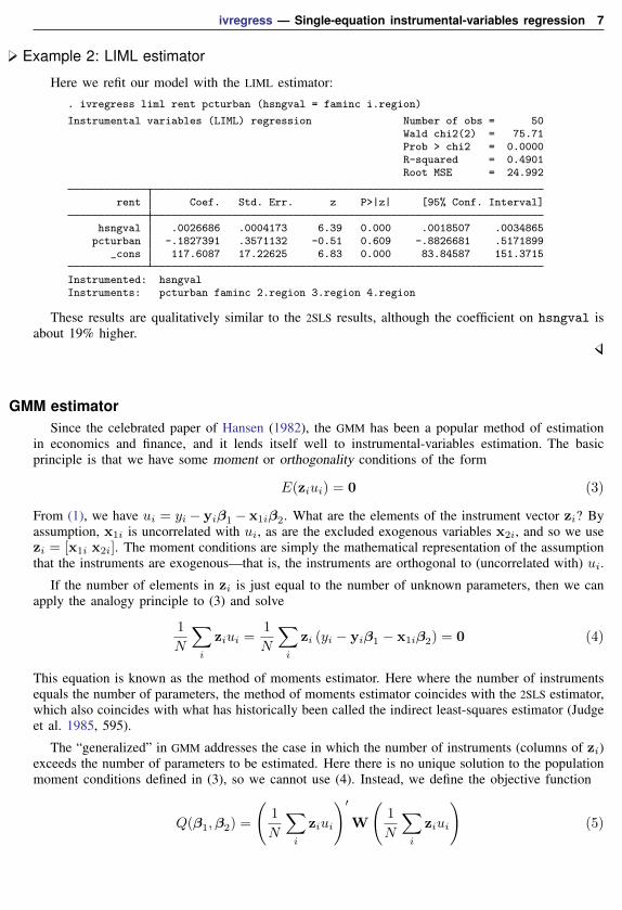
Example 2: LIML estimator

Here we refit our model with the LIML estimator:. ivregress liml rent pcturban (hsngval = faminc i.region)

Instrumental variables (LIML) regression Number of obs = 50Wald chi2(2) = 75.71Prob > chi2 = 0.0000R-squared = 0.4901Root MSE = 24.992

rent Coef. Std. Err. z P>|z| [95% Conf. Interval]

hsngval .0026686 .0004173 6.39 0.000 .0018507 .0034865pcturban -.1827391 .3571132 -0.51 0.609 -.8826681 .5171899

_cons 117.6087 17.22625 6.83 0.000 83.84587 151.3715

Instrumented: hsngvalInstruments: pcturban faminc 2.region 3.region 4.region

These results are qualitatively similar to the 2SLS results, although the coefficient on hsngval isabout 19% higher.

GMM estimatorSince the celebrated paper of Hansen (1982), the GMM has been a popular method of estimation

in economics and finance, and it lends itself well to instrumental-variables estimation. The basicprinciple is that we have some moment or orthogonality conditions of the form

E(ziui) = 0 (3)

From (1), we have ui = yi − yiβ1 − x1iβ2. What are the elements of the instrument vector zi? Byassumption, x1i is uncorrelated with ui, as are the excluded exogenous variables x2i, and so we usezi = [x1i x2i]. The moment conditions are simply the mathematical representation of the assumptionthat the instruments are exogenous—that is, the instruments are orthogonal to (uncorrelated with) ui.

If the number of elements in zi is just equal to the number of unknown parameters, then we canapply the analogy principle to (3) and solve

1

N

∑i

ziui =1

N

∑i

zi (yi − yiβ1 − x1iβ2) = 0 (4)

This equation is known as the method of moments estimator. Here where the number of instrumentsequals the number of parameters, the method of moments estimator coincides with the 2SLS estimator,which also coincides with what has historically been called the indirect least-squares estimator (Judgeet al. 1985, 595).

The “generalized” in GMM addresses the case in which the number of instruments (columns of zi)exceeds the number of parameters to be estimated. Here there is no unique solution to the populationmoment conditions defined in (3), so we cannot use (4). Instead, we define the objective function

Q(β1,β2) =

(1

N

∑i

ziui

)′W

(1

N

∑i

ziui

)(5)

8 ivregress — Single-equation instrumental-variables regression

where W is a positive-definite matrix with the same number of rows and columns as the number ofcolumns of zi. W is known as the weighting matrix, and we specify its structure with the wmatrix()option. The GMM estimator of (β1,β2) minimizes Q(β1,β2); that is, the GMM estimator choosesβ1 and β2 to make the moment conditions as close to zero as possible for a given W. For a moregeneral GMM estimator, see [R] gmm. gmm does not restrict you to fitting a single linear equation,though the syntax is more complex.

A well-known result is that if we define the matrix S0 to be the covariance of ziui and setW = S−10 , then we obtain the optimal two-step GMM estimator, where by optimal estimator we meanthe one that results in the smallest variance given the moment conditions defined in (3).

Suppose that the errors ui are heteroskedastic but independent among observations. Then

S0 = E(ziuiuiz′i) = E(u2i ziz

′i)

and the sample analogue is

S =1

N

∑i

u2i ziz′i (6)

To implement this estimator, we need estimates of the sample residuals ui. ivregress gmm obtainsthe residuals by estimating β1 and β2 by 2SLS and then evaluates (6) and sets W = S−1. Equation (6)is the same as the center term of the “sandwich” robust covariance matrix available from most Stataestimation commands through the vce(robust) option.

Example 3: GMM estimator

Here we refit our model of rents by using the GMM estimator, allowing for heteroskedasticity inui:

. ivregress gmm rent pcturban (hsngval = faminc i.region), wmatrix(robust)

Instrumental variables (GMM) regression Number of obs = 50Wald chi2(2) = 112.09Prob > chi2 = 0.0000R-squared = 0.6616

GMM weight matrix: Robust Root MSE = 20.358

Robustrent Coef. Std. Err. z P>|z| [95% Conf. Interval]

hsngval .0014643 .0004473 3.27 0.001 .0005877 .002341pcturban .7615482 .2895105 2.63 0.009 .1941181 1.328978

_cons 112.1227 10.80234 10.38 0.000 90.95052 133.2949

Instrumented: hsngvalInstruments: pcturban faminc 2.region 3.region 4.region

Because we requested that a heteroskedasticity-consistent weighting matrix be used during estimationbut did not specify the vce() option, ivregress reported standard errors that are robust toheteroskedasticity. Had we specified vce(unadjusted), we would have obtained standard errors thatwould be correct only if the weighting matrix W does in fact converge to S−10 .

ivregress — Single-equation instrumental-variables regression 9

Technical noteMany software packages that implement GMM estimation use the same heteroskedasticity-consistent

weighting matrix we used in the previous example to obtain the optimal two-step estimates but do not usea heteroskedasticity-consistent VCE, even though they may label the standard errors as being “robust”.To replicate results obtained from other packages, you may have to use the vce(unadjusted) option.See Methods and formulas below for a discussion of robust covariance matrix estimation in the GMMframework.

By changing our definition of S0, we can obtain GMM estimators suitable for use with other typesof data that violate the assumption that the errors are independent and identically distributed. Forexample, you may have a dataset that consists of multiple observations for each person in a sample.The observations that correspond to the same person are likely to be correlated, and the estimationtechnique should account for that lack of independence. Say that in your dataset, people are identifiedby the variable personid and you type

. ivregress gmm ..., wmatrix(cluster personid)

Here ivregress estimates S0 as

S =1

N

∑c∈C

qcq′c

where C denotes the set of clusters and

qc =∑i∈cj

uizi

where cj denotes the jth cluster. This weighting matrix accounts for the within-person correlationamong observations, so the GMM estimator that uses this version of S0 will be more efficient thanthe estimator that ignores this correlation.

Example 4: GMM estimator with clustering

We have data from the National Longitudinal Survey on young women’s wages as reported in aseries of interviews from 1968 through 1988, and we want to fit a model of wages as a function ofeach woman’s age and age squared, job tenure, birth year, and level of education. We believe thatrandom shocks that affect a woman’s wage also affect her job tenure, so we treat tenure as endogenous.As additional instruments, we use her union status, number of weeks worked in the past year, and adummy indicating whether she lives in a metropolitan area. Because we have several observations foreach woman (corresponding to interviews done over several years), we want to control for clusteringon each person.

10 ivregress — Single-equation instrumental-variables regression

. use http://www.stata-press.com/data/r13/nlswork(National Longitudinal Survey. Young Women 14-26 years of age in 1968)

. ivregress gmm ln_wage age c.age#c.age birth_yr grade> (tenure = union wks_work msp), wmatrix(cluster idcode)

Instrumental variables (GMM) regression Number of obs = 18625Wald chi2(5) = 1807.17Prob > chi2 = 0.0000R-squared = .

GMM weight matrix: Cluster (idcode) Root MSE = .46951

(Std. Err. adjusted for 4110 clusters in idcode)

Robustln_wage Coef. Std. Err. z P>|z| [95% Conf. Interval]

tenure .099221 .0037764 26.27 0.000 .0918194 .1066227age .0171146 .0066895 2.56 0.011 .0040034 .0302259

c.age#c.age -.0005191 .000111 -4.68 0.000 -.0007366 -.0003016

birth_yr -.0085994 .0021932 -3.92 0.000 -.012898 -.0043008grade .071574 .0029938 23.91 0.000 .0657062 .0774417_cons .8575071 .1616274 5.31 0.000 .5407231 1.174291

Instrumented: tenureInstruments: age c.age#c.age birth_yr grade union wks_work msp

Both job tenure and years of schooling have significant positive effects on wages.

Time-series data are often plagued by serial correlation. In these cases, we can construct a weightingmatrix to account for the fact that the error in period t is probably correlated with the errors in periodst − 1, t − 2, etc. An HAC weighting matrix can be used to account for both serial correlation andpotential heteroskedasticity.

To request an HAC weighting matrix, you specify the wmatrix(hac kernel[

# | opt]) option.

kernel specifies which of three kernels to use: bartlett, parzen, or quadraticspectral. kerneldetermines the amount of weight given to lagged values when computing the HAC matrix, and #denotes the maximum number of lags to use. Many texts refer to the bandwidth of the kernel insteadof the number of lags; the bandwidth is equal to the number of lags plus one. If neither opt nor #is specified, then N − 2 lags are used, where N is the sample size.

If you specify wmatrix(hac kernel opt), then ivregress uses Newey and West’s (1994)algorithm for automatically selecting the number of lags to use. Although the authors’ Monte Carlosimulations do show that the procedure may result in size distortions of hypothesis tests, the procedureis still useful when little other information is available to help choose the number of lags.

For more on GMM estimation, see Baum (2006); Baum, Schaffer, and Stillman (2003, 2007);Cameron and Trivedi (2005); Davidson and MacKinnon (1993, 2004); Hayashi (2000); orWooldridge (2010). See Newey and West (1987) and Wang and Wu (2012) for an introductionto HAC covariance matrix estimation.

ivregress — Single-equation instrumental-variables regression 11

Stored resultsivregress stores the following in e():

Scalarse(N) number of observationse(mss) model sum of squarese(df m) model degrees of freedome(rss) residual sum of squarese(df r) residual degrees of freedome(r2) R2

e(r2 a) adjusted R2

e(F) F statistice(rmse) root mean squared errore(N clust) number of clusterse(chi2) χ2

e(kappa) κ used in LIML estimatore(J) value of GMM objective functione(wlagopt) lags used in HAC weight matrix (if Newey–West algorithm used)e(vcelagopt) lags used in HAC VCE matrix (if Newey–West algorithm used)e(rank) rank of e(V)e(iterations) number of GMM iterations (0 if not applicable)

Macrose(cmd) ivregresse(cmdline) command as typede(depvar) name of dependent variablee(instd) instrumented variablee(insts) instrumentse(constant) noconstant or hasconstant if specifiede(wtype) weight typee(wexp) weight expressione(title) title in estimation outpute(clustvar) name of cluster variablee(hac kernel) HAC kernele(hac lag) HAC lage(vce) vcetype specified in vce()e(vcetype) title used to label Std. Err.e(estimator) 2sls, liml, or gmme(exogr) exogenous regressorse(wmatrix) wmtype specified in wmatrix()e(moments) centered if center specifiede(small) small if small-sample statisticse(depname) depname if depname(depname) specified; otherwise same as e(depvar)e(properties) b Ve(estat cmd) program used to implement estate(predict) program used to implement predicte(footnote) program used to implement footnote displaye(marginsok) predictions allowed by marginse(marginsnotok) predictions disallowed by marginse(asbalanced) factor variables fvset as asbalancede(asobserved) factor variables fvset as asobserved

Matricese(b) coefficient vectore(Cns) constraints matrixe(W) weight matrix used to compute GMM estimatese(S) moment covariance matrix used to compute GMM variance–covariance matrixe(V) variance–covariance matrix of the estimatorse(V modelbased) model-based variance

Functionse(sample) marks estimation sample

12 ivregress — Single-equation instrumental-variables regression

Methods and formulasMethods and formulas are presented under the following headings:

Notation2SLS and LIML estimatorsGMM estimator

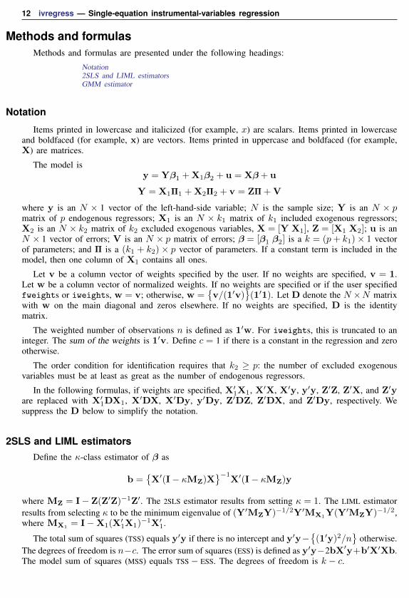
Notation

Items printed in lowercase and italicized (for example, x) are scalars. Items printed in lowercaseand boldfaced (for example, x) are vectors. Items printed in uppercase and boldfaced (for example,X) are matrices.

The model isy = Yβ1 +X1β2 + u = Xβ+ u

Y = X1Π1 +X2Π2 + v = ZΠ+V

where y is an N × 1 vector of the left-hand-side variable; N is the sample size; Y is an N × pmatrix of p endogenous regressors; X1 is an N × k1 matrix of k1 included exogenous regressors;X2 is an N × k2 matrix of k2 excluded exogenous variables, X = [Y X1], Z = [X1 X2]; u is anN × 1 vector of errors; V is an N × p matrix of errors; β = [β1 β2] is a k = (p+ k1)× 1 vectorof parameters; and Π is a (k1 + k2)× p vector of parameters. If a constant term is included in themodel, then one column of X1 contains all ones.

Let v be a column vector of weights specified by the user. If no weights are specified, v = 1.Let w be a column vector of normalized weights. If no weights are specified or if the user specifiedfweights or iweights, w = v; otherwise, w =

{v/(1′v)

}(1′1). Let D denote the N ×N matrix

with w on the main diagonal and zeros elsewhere. If no weights are specified, D is the identitymatrix.

The weighted number of observations n is defined as 1′w. For iweights, this is truncated to aninteger. The sum of the weights is 1′v. Define c = 1 if there is a constant in the regression and zerootherwise.

The order condition for identification requires that k2 ≥ p: the number of excluded exogenousvariables must be at least as great as the number of endogenous regressors.

In the following formulas, if weights are specified, X′1X1, X′X, X′y, y′y, Z′Z, Z′X, and Z′yare replaced with X′1DX1, X′DX, X′Dy, y′Dy, Z′DZ, Z′DX, and Z′Dy, respectively. Wesuppress the D below to simplify the notation.

2SLS and LIML estimatorsDefine the κ-class estimator of β as

b ={X′(I− κMZ)X

}−1X′(I− κMZ)y

where MZ = I−Z(Z′Z)−1Z′. The 2SLS estimator results from setting κ = 1. The LIML estimatorresults from selecting κ to be the minimum eigenvalue of (Y′MZY)−1/2Y′MX1

Y(Y′MZY)−1/2,where MX1

= I−X1(X′1X1)

−1X′1.

The total sum of squares (TSS) equals y′y if there is no intercept and y′y−{(1′y)2/n

}otherwise.

The degrees of freedom is n−c. The error sum of squares (ESS) is defined as y′y−2bX′y+b′X′Xb.The model sum of squares (MSS) equals TSS− ESS. The degrees of freedom is k − c.

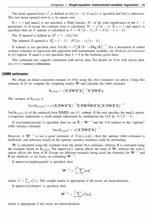
ivregress — Single-equation instrumental-variables regression 13

The mean squared error, s2, is defined as ESS/(n− k) if small is specified and ESS/n otherwise.The root mean squared error is s, its square root.

If c = 1 and small is not specified, a Wald statistic, W , of the joint significance of the k − 1parameters of β except the constant term is calculated; W ∼ χ2(k − 1). If c = 1 and small isspecified, then an F statistic is calculated as F =W/(k − 1); F ∼ F (k − 1, n− k).

The R-squared is defined as R2 = 1− ESS/TSS.

The adjusted R-squared is R2a = 1− (1−R2)(n− c)/(n− k).

If robust is not specified, then Var(b) = s2{X′(I − κMZ)X

}−1. For a discussion of robust

variance estimates in regression and regression with instrumental variables, see Methods and formulasin [R] regress. If small is not specified, then k = 0 in the formulas given there.

This command also supports estimation with survey data. For details on VCEs with survey data,see [SVY] variance estimation.

GMM estimator

We obtain an initial consistent estimate of β by using the 2SLS estimator; see above. Using thisestimate of β, we compute the weighting matrix W and calculate the GMM estimator

bGMM ={X′ZWZ′X

}−1X′ZWZ′y

The variance of bGMM is

Var(bGMM) = n{X′ZWZ′X

}−1X′ZWSWZ′X

{X′ZWZ′X

}−1Var(bGMM) is of the sandwich form DMD; see [P] robust. If the user specifies the small option,ivregress implements a small-sample adjustment by multiplying the VCE by N/(N − k).

If vce(unadjusted) is specified, then we set S = W−1 and the VCE reduces to the “optimal”GMM variance estimator

Var(βGMM) = n{X′ZWZ′X

}−1However, if W−1 is not a good estimator of E(ziuiuiz

′i), then the optimal GMM estimator is

inefficient, and inference based on the optimal variance estimator could be misleading.

W is calculated using the residuals from the initial 2SLS estimates, whereas S is estimated usingthe residuals based on bGMM. The wmatrix() option affects the form of W, whereas the vce()option affects the form of S. Except for different residuals being used, the formulas for W−1 andS are identical, so we focus on estimating W−1.

If wmatrix(unadjusted) is specified, then

W−1 =s2

n

∑i

ziz′i

where s2 =∑i u

2i /n. This weight matrix is appropriate if the errors are homoskedastic.

If wmatrix(robust) is specified, then

W−1 =1

n

∑i

u2i ziz′i

which is appropriate if the errors are heteroskedastic.

14 ivregress — Single-equation instrumental-variables regression

If wmatrix(cluster clustvar) is specified, then

W−1 =1

n

∑c

qcq′c

where c indexes clusters,qc =

∑i∈cj

uizi

and cj denotes the jth cluster.

If wmatrix(hac kernel[

#]) is specified, then

W−1 =1

n

∑i

u2i ziz′i +

1

n

l=n−1∑l=1

i=n∑i=l+1

K(l,m)uiui−l(ziz′i−l + zi−lz

′i

)where m = # if # is specified and m = n− 2 otherwise. Define z = l/(m+ 1). If kernel is nwest,then

K(l,m) ={1− z 0 ≤ z ≤ 10 otherwise

If kernel is gallant, then

K(l,m) =

{1− 6z2 + 6z3 0 ≤ z ≤ 0.52(1− z)3 0.5 < z ≤ 10 otherwise

If kernel is quadraticspectral, then

K(l,m) =

{1 z = 03 {sin(θ)/θ − cos(θ)} /θ2 otherwise

where θ = 6πz/5.

If wmatrix(hac kernel opt) is specified, then ivregress uses Newey and West’s (1994) automaticlag-selection algorithm, which proceeds as follows. Define h to be a (k1 + k2)× 1 vector containingones in all rows except for the row corresponding to the constant term (if present); that row containsa zero. Define

fi = (uizi)h

σj =1

n

n∑i=j+1

fifi−j j = 0, . . . ,m∗

s (q) = 2

m∗∑j=1

σjjq

s (0) = σ0 + 2

m∗∑j=1

σj

γ = cγ

{(s (q)

s (0)

)2}1/2q+1

m = γn1/(2q+1)

ivregress — Single-equation instrumental-variables regression 15

where q, m∗, and cγ depend on the kernel specified:

Kernel q m∗ cγ

Bartlett 1 int{

20(T/100)2/9}

1.1447

Parzen 2 int{

20(T/100)4/25}

2.6614

Quadratic spectral 2 int{

20(T/100)2/25}

1.3221

where int(x) denotes the integer obtained by truncating x toward zero. For the Bartlett and Parzenkernels, the optimal lag is min{int(m),m∗}. For the quadratic spectral, the optimal lag is min{m,m∗}.

If center is specified, when computing weighting matrices ivregress replaces the term uizi inthe formulas above with uizi − uz, where uz =

∑i uizi/N .

ReferencesAndrews, D. W. K. 1991. Heteroskedasticity and autocorrelation consistent covariance matrix estimation. Econometrica

59: 817–858.

Angrist, J. D., and J.-S. Pischke. 2009. Mostly Harmless Econometrics: An Empiricist’s Companion. Princeton, NJ:Princeton University Press.

Basmann, R. L. 1957. A generalized classical method of linear estimation of coefficients in a structural equation.Econometrica 25: 77–83.

Bauldry, S. 2014. miivfind: A command for identifying model-implied instrumental variables for structural equationmodels in Stata. Stata Journal 14: 60–75.

Baum, C. F. 2006. An Introduction to Modern Econometrics Using Stata. College Station, TX: Stata Press.

Baum, C. F., M. E. Schaffer, and S. Stillman. 2003. Instrumental variables and GMM: Estimation and testing. StataJournal 3: 1–31.

. 2007. Enhanced routines for instrumental variables/generalized method of moments estimation and testing. StataJournal 7: 465–506.

Cameron, A. C., and P. K. Trivedi. 2005. Microeconometrics: Methods and Applications. New York: CambridgeUniversity Press.

. 2010. Microeconometrics Using Stata. Rev. ed. College Station, TX: Stata Press.

Davidson, R., and J. G. MacKinnon. 1993. Estimation and Inference in Econometrics. New York: Oxford UniversityPress.

. 2004. Econometric Theory and Methods. New York: Oxford University Press.

Desbordes, R., and V. Verardi. 2012. A robust instrumental-variables estimator. Stata Journal 12: 169–181.

Finlay, K., and L. M. Magnusson. 2009. Implementing weak-instrument robust tests for a general class of instrumental-variables models. Stata Journal 9: 398–421.

Gallant, A. R. 1987. Nonlinear Statistical Models. New York: Wiley.

Greene, W. H. 2012. Econometric Analysis. 7th ed. Upper Saddle River, NJ: Prentice Hall.

Hall, A. R. 2005. Generalized Method of Moments. Oxford: Oxford University Press.

Hansen, L. P. 1982. Large sample properties of generalized method of moments estimators. Econometrica 50:1029–1054.

Hayashi, F. 2000. Econometrics. Princeton, NJ: Princeton University Press.

Judge, G. G., W. E. Griffiths, R. C. Hill, H. Lutkepohl, and T.-C. Lee. 1985. The Theory and Practice of Econometrics.2nd ed. New York: Wiley.

Kmenta, J. 1997. Elements of Econometrics. 2nd ed. Ann Arbor: University of Michigan Press.

Koopmans, T. C., and W. C. Hood. 1953. Studies in Econometric Method. New York: Wiley.

16 ivregress — Single-equation instrumental-variables regression

Koopmans, T. C., and J. Marschak. 1950. Statistical Inference in Dynamic Economic Models. New York: Wiley.

Newey, W. K., and K. D. West. 1987. A simple, positive semi-definite, heteroskedasticity and autocorrelation consistentcovariance matrix. Econometrica 55: 703–708.

. 1994. Automatic lag selection in covariance matrix estimation. Review of Economic Studies 61: 631–653.

Nichols, A. 2007. Causal inference with observational data. Stata Journal 7: 507–541.

Palmer, T. M., V. Didelez, R. R. Ramsahai, and N. A. Sheehan. 2011. Nonparametric bounds for the causal effectin a binary instrumental-variable model. Stata Journal 11: 345–367.

Poi, B. P. 2006. Jackknife instrumental variables estimation in Stata. Stata Journal 6: 364–376.

Stock, J. H., and M. W. Watson. 2011. Introduction to Econometrics. 3rd ed. Boston: Addison–Wesley.

Stock, J. H., J. H. Wright, and M. Yogo. 2002. A survey of weak instruments and weak identification in generalizedmethod of moments. Journal of Business and Economic Statistics 20: 518–529.

Theil, H. 1953. Repeated Least Squares Applied to Complete Equation Systems. Mimeograph from the CentralPlanning Bureau, The Hague.

Wang, Q., and N. Wu. 2012. Long-run covariance and its applications in cointegration regression. Stata Journal 12:515–542.

Wooldridge, J. M. 2010. Econometric Analysis of Cross Section and Panel Data. 2nd ed. Cambridge, MA: MIT Press.

. 2013. Introductory Econometrics: A Modern Approach. 5th ed. Mason, OH: South-Western.

Wright, P. G. 1928. The Tariff on Animal and Vegetable Oils. New York: Macmillan.

Also see[R] ivregress postestimation — Postestimation tools for ivregress

[R] gmm — Generalized method of moments estimation

[R] ivprobit — Probit model with continuous endogenous regressors

[R] ivtobit — Tobit model with continuous endogenous regressors

[R] reg3 — Three-stage estimation for systems of simultaneous equations

[R] regress — Linear regression

[SEM] intro 5 — Tour of models

[SVY] svy estimation — Estimation commands for survey data

[TS] forecast — Econometric model forecasting

[XT] xtivreg — Instrumental variables and two-stage least squares for panel-data models

[U] 20 Estimation and postestimation commands